Multi-Strategy Enhanced Beaver Behavior Optimizer for Global Optimization and Enterprise Bankruptcy Prediction

Abstract

Enterprise bankruptcy prediction is a critical research issue in financial risk early warning, credit evaluation, and investment decision-making. To address the limitations of traditional methods in handling high-dimensional, nonlinear, and complex financial data, including parameter sensitivity, susceptibility to local optima, and insufficient prediction stability, this study proposes a multi-strategy enhanced Beaver Behavior Optimizer and applies it to optimize kernel extreme learning machines, constructing the MEBBO KELM prediction model. Three improvement mechanisms are introduced, including an elite pool enhanced exploration strategy, a stochastic centroid reverse learning strategy, and a leader guided boundary control strategy, which improve population diversity, global search capability, boundary handling capacity, and convergence accuracy. The proposed algorithm is evaluated on CEC2017 and CEC2022 benchmark datasets and compared with EWOA, HPHHO, MELGWO, TACPSO, CFOA, ALA, AOO, RIME, and BBO. Statistical analyses are conducted using the Wilcoxon rank sum test and the Friedman test. The results demonstrate that MEBBO achieves superior solution accuracy and stability, indicating strong global optimization capability and robustness. Further experiments on the Wieslaw Corporate Bankruptcy Dataset show that MEBBO-KELM achieves strong and robust performance across multiple evaluation metrics, including ACC, MCC, Sensitivity, Specificity, Precision, Recall, and F1 score. Specifically, ACC reaches 79.7578, MCC reaches 0.6050, and F1 score reaches 78.8504, confirming its effectiveness.

1. Introduction

Enterprise bankruptcy prediction has long been a core issue in financial risk management, credit evaluation, investment decision-making, and prudential regulation. Its primary objective lies in identifying potential financial distress or bankruptcy risks through corporate financial indicators, operational conditions, and governance characteristics [1]. With the continuous evolution of capital markets, increasingly complex business environments, and heightened external uncertainties, bankruptcy prediction has transcended its role as a post-event analytical tool to become a critical mechanism for proactive risk warning and resource allocation [2]. For creditors, accurate bankruptcy prediction facilitates optimized credit approval processes and post-loan risk control; for investors, it helps identify potential value traps and enhance asset allocation efficiency; while for regulators, it strengthens risk monitoring capabilities and reduces risk contagion probabilities [3]. Therefore, developing bankruptcy prediction models with higher predictive accuracy, stronger generalization capabilities, and improved robustness remains a pivotal research focus in interdisciplinary studies spanning finance, management, and intelligent computing.

Current research on bankruptcy prediction primarily follows two technical approaches: parametric methods and non-parametric methods [4]. Parametric methods include multivariate discriminant analysis, logistic regression, and Probit models. While these approaches offer clear statistical frameworks and strong interpretability, they often rely on assumptions about data distribution, variable independence, or linear relationships, leading to limitations when handling high-dimensional, nonlinear, or noisy datasets [5,6]. In contrast, non-parametric methods such as support vector machines, decision trees, random forests, artificial neural networks, and deep learning models demonstrate greater adaptability to prior distribution assumptions. They effectively capture complex nonlinear relationships between variables, making them widely adopted in bankruptcy prediction studies with robust predictive performance [7,8]. However, these methods remain highly sensitive to parameter settings, feature redundancy, and training processes, frequently resulting in local optimization traps [9]. Consequently, developing effective optimization mechanisms to enhance model performance and classification accuracy has become crucial for advancing bankruptcy prediction research [10,11]. Recent years have seen meta-heuristic algorithms emerge as promising solutions, leveraging their global search capabilities, flexibility, and adaptability to feature selection and joint parameter optimization [12].

Meta-heuristic algorithms can generally be categorized into four major types [13]: Swarm Intelligence (SI), Evolutionary Algorithms (EA), Physics-based Algorithms (PhA), and Human-based Algorithms. Among these, Swarm Intelligence algorithms are primarily inspired by the cooperative behaviors of social biological groups, which have evolved through natural processes over time [14]. For instance, the Particle Swarm Optimization (PSO) algorithm proposed by Kennedy and Eberhart in 1995 was developed based on the natural movement patterns of swarm particles [15]. Evolutionary Algorithms represent probabilistic optimization methods grounded in natural evolutionary principles [16], with the Genetic Algorithm (GA) introduced by Holland [17] in 1992 serving as a classic example derived from Darwinian evolution theory. Physics-based Algorithms are primarily derived from physical laws or chemical reaction processes. For instance, the Simulated Annealing (SA) algorithm proposed by Kirkpatrick, Gelatt Jr., and Vecchi [18] in 1983 was inspired by the thermal equilibrium behavior of multi-degree-of-freedom systems at finite temperatures. Human behavior-based algorithms primarily simulate human activities or social interaction processes. A notable example is the Harmony Search (HS) algorithm introduced by Zong Woo et al. [19] in 2001, which mimics the collaborative mechanisms observed during musicians’ improvisational performances.

The Beaver Behavior Optimizer (BBO) is a newly proposed swarm intelligence optimization algorithm inspired by the behavioral mechanisms of beavers in dam construction, material transport, and collaborative activities [20]. By simulating the cooperative processes of beaver colonies in environmental contexts, this algorithm achieves both global exploration and local exploitation of search spaces. Although the original BBO demonstrated promising application potential in various benchmark tests and engineering optimization tasks, the No Free Lunch (NFL) theorem indicates that no optimization algorithm can maintain optimal performance across all problems [21,22]. Similarly, in bankruptcy prediction tasks characterized by high-dimensional features, complex nonlinear relationships, and noise interference, the original BBO still exhibits issues such as slow convergence rates and insufficient optimization accuracy [23]. To address these limitations, this paper proposes a Multi-Strategy Enhanced Beaver Behavior Optimizer (MEBBO). The primary contributions of this study are reflected in the following aspects:

(1)

We propose MEBBO by embedding three targeted strategies into the key search stages of the original BBO, establishing a one-to-one correspondence between the proposed mechanisms and BBO’s main weaknesses, including insufficient search guidance, weak local-optimum escape ability, and inefficient boundary handling.

(2)

We design an elite pool-enhanced exploration strategy, which constructs an elite pool from high-quality individuals and embeds elite-guided learning into the architect update process, thereby improving search directionality and reducing the blind search caused by randomly selected learning objects in the original BBO.

(3)

We introduce a stochastic centroid reverse learning strategy, which generates reverse candidate solutions based on centroids formed by randomly selected individuals, thereby enhancing search-space expansion and local-optimum escape ability, and addressing the lack of effective reverse learning or backtracking mechanisms when the original BBO population is trapped in local regions.

(4)

We develop a leader-guided boundary control strategy, which redirects boundary-crossing individuals into the feasible domain under the guidance of the current best individual, thereby improving boundary correction stability and avoiding search-direction disruption and boundary aggregation caused by direct truncation in the original BBO.

(5)

This study integrates the three strategies into a coordinated search framework, in which elite pool-enhanced exploration strengthens search guidance, stochastic centroid reverse learning expands the solution space, and leader-guided boundary control improves feasibility correction, enabling MEBBO to better balance exploration, exploitation, diversity maintenance, and boundary handling.

(6)

This study systematically evaluates MEBBO on CEC2017 and CEC2022 benchmark test suites and further integrates it with KELM for enterprise bankruptcy prediction, verifying its optimization accuracy, robustness, and practical applicability in financial risk classification.

The remainder of this paper is organized as follows: Section 2 reviews recent literature on meta-heuristic optimization algorithms; Section 3 introduces the original BBO algorithm and elaborates on the proposed multi-strategy enhanced BBO algorithm; Section 4 presents numerical experiments and analysis; Section 5 presents bankruptcy prediction and indicator analysis based on the MEBBO-KELM model; Section 6 discusses the advantages, original contributions, and limitations of the proposed method in comparison with related approaches; Section 7 summarizes the key research findings and proposes potential directions for future research.

2. Related Work

Meta-heuristic algorithms, as a class of stochastic optimization methods inspired by nature, have been widely applied in predictive modeling in recent years. By simulating biological evolution, population behavior, or physical processes, these algorithms can effectively address high-dimensional, nonlinear, and non-convex prediction problems, thereby compensating for the limitations of traditional prediction methods in modeling complex systems [23].

In recent years, researchers have developed various novel meta-heuristic algorithms addressing different natural phenomena and biological behaviors, applying them to diverse prediction tasks. Wei et al. [24] proposed a multi-objective escape bird search optimization algorithm integrated with a Transformer for stock market forecasting. Results demonstrated that this method effectively balances global exploration and local exploitation, outperforming traditional optimization algorithms in stock price prediction tasks. Yu et al. [25] proposed an enhanced version of the dung beetle optimization algorithm for optimizing the path of unmanned aerial vehicles. The experimental results show that this algorithm accelerates the convergence speed through multiple mechanisms and improves the optimization accuracy at the same time. Combining meta-heuristic algorithms with deep learning models to optimize network hyperparameters or structural parameters has become a key research trend in recent years. Elshewey et al. [26] utilized the grey goose optimization algorithm for automatic parameter tuning of LSTM networks, significantly improving model accuracy in cardiac disease classification prediction. Wei et al. [24] further applied improved meta-heuristic algorithms to optimize the parameters of the Transformer’s attention mechanism, achieving remarkable stock market prediction accuracy and highlighting the strong potential of meta-heuristic algorithms in deep learning model optimization. In feature selection, meta-heuristic algorithms can effectively eliminate redundant features, reduce dimensionality, and enhance model generalization capabilities. Abualhaj et al. [27] integrated the Grey Wolf Optimization Algorithm with Random Forest to develop the RFGWO-Mal malware detection system, achieving high detection accuracy on the Obfuscated-MalMem2022 dataset. Abualhaj et al. [28] compared Whale Optimization Algorithm and Harris Hawk Optimization Algorithm in intrusion detection feature selection, demonstrating that both methods maintained high classification accuracy while significantly reducing dimensionality, thereby validating the effectiveness of meta-heuristic feature selection. Additionally, hybrid prediction frameworks combining multiple meta-heuristic algorithms have emerged as a research hotspot. Hai et al. [29] proposed a computational intelligence framework integrating neural networks, gene expression programming, and multi-objective particle swarm optimization for ternary hybrid nanofluid performance prediction, achieving high prediction accuracy. Giedraityte et al. [23] systematically summarized hybrid meta-heuristic prediction optimization methods for renewable energy systems, highlighting that integrated applications of multi-objective particle swarm optimization, NSGA-II, and Grey Wolf Optimization algorithms enhance system economic efficiency, environmental sustainability, and reliability.

In the field of bankruptcy prediction, traditional statistical models and machine learning methods often face challenges related to parameter optimization and limited predictive accuracy when processing high-dimensional, nonlinear, and imbalanced financial data. To address these issues, researchers have begun incorporating meta-heuristic algorithms into bankruptcy prediction model optimization. Jiang et al. [30] proposed an improved Condor Optimization Algorithm (TIS-NGO) that integrates innovative thinking mechanisms, differential evolutionary heuristic attack strategies, and centroid-based opposing boundary control, and applied it to optimize KELM for constructing bankruptcy prediction models. Results demonstrated that this method exhibited excellent convergence performance and classification accuracy on both benchmark tests and bankruptcy datasets. Khaldi et al. [31] improved arithmetic optimization algorithms based on S-shaped opposing learning strategies and applied them to corporate financial failure prediction. Experimental results showed that this approach enhanced population diversity, expanded the search scope, and achieved superior prediction outcomes compared to the original algorithms. To tackle data imbalance in bankruptcy prediction, Ainan et al. [32] proposed a hybrid model combining XGBoost and Artificial Neural Networks (ANN) with genetic algorithm parameter optimization. The results indicated that this method achieved high AUC, sensitivity, and accuracy on an imbalanced Polish enterprise dataset, significantly improving bankruptcy prediction reliability. Meanwhile, KELM has become a widely used classification model in recent years because of its fast training speed and strong generalization capabilities. However, its performance remains highly dependent on parameter settings, making meta-heuristic algorithms essential for parameter optimization. In addition to Jiang et al. [30], Zhu et al. [33] proposed an improved secretary bird optimization algorithm for KELM optimization. Although applied to diabetes classification, their framework demonstrates that meta-heuristic KELM optimization exhibits strong versatility in classification prediction tasks. Beyond parameter optimization, meta-heuristic algorithms are also widely used for feature selection in bankruptcy prediction. Peng et al. [34] introduced a hierarchical Harris eagle optimization algorithm for high-dimensional feature selection, validating its effectiveness across multiple datasets. Zhou et al. [35] developed a slime mold algorithm combining enhanced local variation and full neighborhood search, outperforming traditional meta-heuristic algorithms in feature selection tasks. Ji et al. [36] proposed an improved roulette optimization technique (RMRIME), which enhances convergence accuracy and improves model classification performance on bankruptcy prediction datasets through roulette selection and elite information-guided variation to expand the search space.

3. Materials and Methods

This section presents the methodological foundation of the study. It first introduces the original BBO algorithm to provide the necessary background for understanding its search mechanism and limitations. Then, the proposed MEBBO algorithm is described in detail, including the design logic, mathematical formulation, and implementation process of the three enhancement strategies. This organization enables readers to understand how the proposed method is developed from the original BBO and why each improvement strategy is introduced.

3.1. An Overview of BBO

The BBO is a novel swarm intelligence optimization algorithm inspired by the cooperative dam-building behavior of beavers. The following formulation is mainly based on the original BBO framework proposed by Ouyang et al. [20]. Its core concept involves mapping two typical behaviors—material collection and dam maintenance—during beaver dam construction into two distinct phases: global exploration and local exploitation in the optimization process. Each individual’s decision variables are treated as attributes of specific “building materials,” with different individuals representing unique material combinations carried by beavers. By simulating beavers’ behavior of extensively searching for materials in the early stages and continuously maintaining and improving the dam structure in later stages, the algorithm achieves efficient exploration of the solution space and approximation of the optimal solution. BBO features a clear division between the exploration and exploitation phases, strong stochastic search capabilities, effective suppression of premature convergence, and enhanced convergence accuracy.

For consistency, the position of the i-th beaver individual at iteration $t$ is denoted as $x_i^t=\left(x_{i,1}^t,x_{i,2}^t,\cdots ,x_{i,D}^t\right)$, where $D$ is the problem dimension. BBO initially initializes the population through a stochastic approach. For the i-th individual, the initial position in the j-th dimension is determined by a random value drawn between the lower and upper bounds:

$$x_{i,j}=l{b}_j+(u{b}_j-l{b}_j)\cdot rand,$$

(1)

where $l{b}_j$ and $u{b}_j$ denote the lower and upper bounds of the j-th dimension, respectively, and $rand\in [0,1]$ denotes a uniformly distributed random number. To characterize the dynamic transition of the algorithm from exploration to exploitation, the authors further define the dam-phase factor:

$$E=\mathit{sin}\left({\displaystyle \frac{\pi t}{2T}}\right),$$

(2)

where $t$ represents the current iteration count, and $T$ represents the maximum iteration count. As the iterations progress, the value of $E$ monotonically increases from 0 to 1. In each iteration, a random number is generated. When the condition is met, the algorithm enters the exploitation phase; otherwise, it enters the exploration phase. This design enables the algorithm to prioritize local fine-tuning in the later stages while maintaining a certain level of global search capability.

During the exploration phase, the population is divided into two categories of individuals: the top 25% in terms of fitness are defined as architects, while the remainder are prospectors. Architect individuals update their current positions by learning from other elite individuals, with the update formula being:

$$x_{i,j}^{architect}(t+1)=x_{i,j}^{architect}(t)+I(r_2<0.5)r_3\left(x_{k,j}^{architect}(t)-x_{i,j}^{architect}(t)\right),$$

(3)

where $I(·)$ denotes the characteristic function, $r_2,r_3\in [0,1]$ are random numbers, and $k$ indicates another architect individual selected at random. For a prospector individual, it learns from an architect while actively exploring new materials through a random term with Gaussian perturbation. Its update formula is as follows:

$$x_{i,j}^{prospector}(t+1)=x_{i,j}^{prospector}(t)+I(r_4<0.5)\hspace{0.17em}{r}_5\left(x_{i,j}^{\mathrm{a}rchitect}(t)-x_{i,j}^{prospector}(t)\right)+{\displaystyle \frac{r_6\cos \left(\frac{\pi t}{2T}\right)(u{b}_j-l{b}_j)}{10}}$$

(4)

where $r_4,r_5\in [0,1]$ are uniformly distributed random numbers, and $r_6$ denotes a Gaussian random variable. Consequently, BBO integrates both elite guidance and stochastic diffusion during the exploration phase, which enhances population diversity and prevents falling into local optima.

During the exploitation phase, all individuals are treated as architects and perform refinement searches around the current optimal solution. The update formula is as follows:

$$x_{i,j}^{architect}(t+1)=x_{i,j}^{architect}(t)+r_7\left(x_{k,j}^{architect}(t)-x_{i,j}^{architect}(t)\right)+r_8\left(x_{best,j}^{architect}(t)-x_{i,j}^{architect}(t)\right)$$

(5)

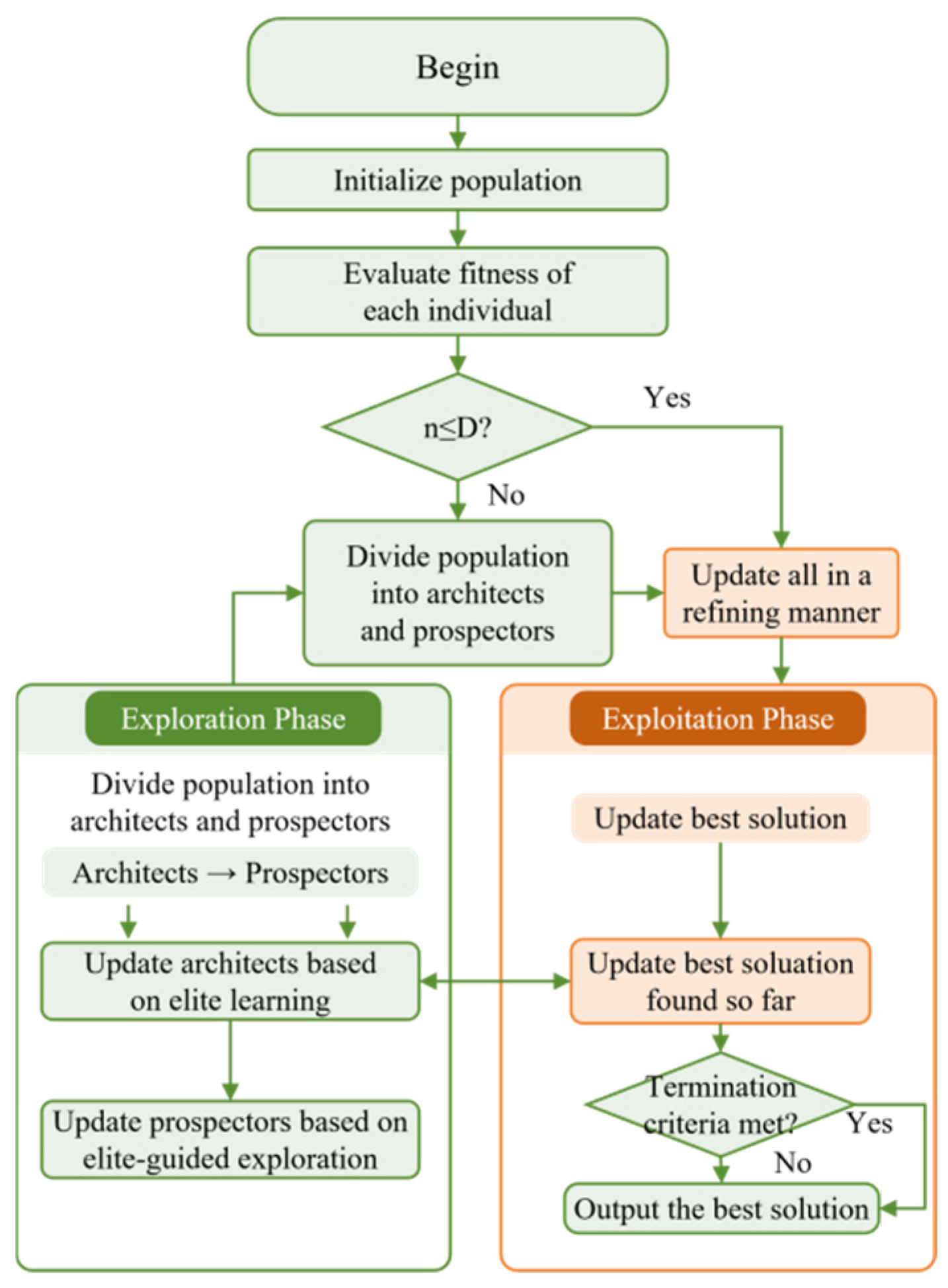
where $r_7,r_8\in [0,1]$ are random numbers, and $x_{best,j}^{architect}(t)$ denotes the position of the current global best individual in the j-th dimension. This equation indicates that during the local exploitation phase, individuals are simultaneously guided by both random peer individuals and the global optimal individual, thereby enhancing local refinement capabilities. In summary, the basic steps of BBO include population initialization, fitness calculation, determining whether to enter the exploration or exploitation phase based on the dam-phase factor, updating individual positions according to the corresponding formulas, and iterating until the termination conditions are met to output the optimal solution. The flowchart of the original BBO algorithm is shown in Figure 1.

3.2. The Proposed MEBBO

Although the original BBO has shown promising optimization potential in continuous optimization problems, its search mechanism still has several structural limitations when dealing with complex, high-dimensional, and multimodal problems. Specifically, the random selection of learning objects may lead to insufficient search guidance and unstable population evolution; the lack of an effective search-space expansion mechanism may weaken the algorithm’s ability to escape local optima; and the simple boundary handling strategy may reduce the quality of infeasible-solution correction. These limitations can result in population diversity loss, premature convergence, and insufficient optimization accuracy. Therefore, there remains a clear need to improve the original BBO by developing a more coordinated search mechanism that can simultaneously enhance exploration, maintain diversity, and improve boundary correction.

Although recent variants such as CCBBO and EBBO have attempted to improve BBO through crisscross information exchange or multi-stage cooperative mechanisms [37,38], the application of a BBO-based enhanced optimizer to KELM parameter tuning in bankruptcy prediction remains insufficiently explored.

Table 1. Comparison between MEBBO and recent BBO variants.

Algorithm	Main Strategies	Main Application	Difference from MEBBO
Original BBO [20]	Material gathering; dam maintenance	Solar PV and engineering problems	Baseline BBO framework
CCBBO [37]	Crisscross strategy	Global optimization; oil reservoir production	Focuses on dimension-wise information exchange
EBBO [38]	Adaptive mutation; dynamic OBL; risk-aware decision	Engineering optimization	Focuses on multi-stage cooperation and constraint handling
MEBBO	Elite pool exploration; stochastic centroid reverse learning; leader-guided boundary control	Global optimization and bankruptcy prediction	Tailored to BBO’s exploration blindness, lack of backtracking, and boundary clustering; further integrated with KELM for financial classification

summarizes the main differences between MEBBO and recent BBO variants.

To address this research gap, this subsection presents the proposed Multi-Strategy Enhanced Beaver Behavior Optimizer (MEBBO). The main purpose is to explain how the original BBO is improved through three complementary strategies designed for different stages and weaknesses of the search process. First, an elite pool-enhanced exploration strategy is introduced to improve the quality of search guidance and enhance global exploration. Second, a stochastic centroid reverse learning strategy is developed to expand the solution space and strengthen the ability to escape local optima. Third, a leader-guided boundary control strategy is designed to improve the correction of out-of-bound individuals and enhance convergence stability. Through this organization, this subsection clarifies the design logic, mathematical formulation, and implementation process of MEBBO.

Compared with existing BBO variants such as CCBBO and EBBO, the proposed MEBBO differs not only in the specific improvement strategies adopted but also in the way these strategies are embedded into the original BBO search mechanism. CCBBO mainly improves BBO through crisscross information exchange, while EBBO focuses on adaptive mutation, dynamic opposition-based learning, and multi-stage cooperation. In contrast, MEBBO is designed according to the specific weaknesses observed in the original BBO search process: the elite pool-enhanced exploration strategy improves the quality of learning objects in the exploration phase, the stochastic centroid reverse learning strategy provides a dynamic backtracking mechanism based on population distribution, and the leader-guided boundary control strategy transforms passive boundary truncation into informative feasibility correction. Therefore, MEBBO is not merely another variant that adds general enhancement operators to BBO, but a coordinated framework that establishes explicit correspondence between BBO’s search limitations and targeted improvement mechanisms.

3.2.1. Elite Pool-Enhanced Exploration

In the original BBO algorithm, an individual architect typically selects a random member from the architect set for learning, with its update mechanism expressed as

$$x_{i,j}^{t+1}=x_{i,j}^t+r\left(x_{k,j}^t-x_{i,j}^t\right)$$

(6)

where $x_{i,j}^t$ denotes the position of an individual in dimension $j$ at the $t$-th iteration, $x_{k,j}^t$ represents the position of a randomly selected architect individual in dimension $j$, and $r\in (0,1)$ is a random number. Although this mechanism retains a certain degree of randomness, the complete randomness of learning objects leads to unstable reference information quality, which can easily result in blind search directions and consequently affect the algorithm’s convergence efficiency and solution accuracy.

To enhance the utilization of high-quality solution information during the exploration phase, this paper introduces an elite pool-enhanced exploration strategy. Specifically, in each iteration, the population is first ranked according to individual fitness values, and the top-ranked individuals are selected to form the elite pool. Let the population size be $N$. Then, the elite pool size is defined as

$$N_e=\mathrm{r}\mathrm{o}\mathrm{u}\mathrm{n}\mathrm{d}(0.2N)$$

(7)

Accordingly, the elite pool in the $t$-th generation can be expressed as

$${EP}^t=\left\{x_{\mathrm{e},1}^t,x_{\mathrm{e},2}^t,\dots ,x_{\mathrm{e},N_e}^t\right\}$$

(8)

where ${EP}^t$ denotes the elite pool at iteration $t$, and $x_{\mathrm{e},\mathrm{k}}^t$ represents the $k$-th elite individual selected according to fitness ranking. During the architect update phase, instead of randomly selecting learning objects from the general architect set, an elite individual is randomly selected from the elite pool for guidance. Its update formula is as follows:

$$x_{i,j}^{t+1}=x_{i,j}^t+r\left(x_{e,j}^t-x_{i,j}^t\right)$$

(9)

Unlike single-optimum solution guidance, this strategy employs a “random elite pool selection” mechanism, enabling individuals to learn from multiple high-quality solutions. This approach not only enhances the utilization of advantageous regions but also prevents the population from rapidly converging on a single point, thereby achieving a balance between optimum information utilization and population diversity maintenance.

The elite pool enhancement exploration strategy demonstrates three key advantages. First, it confines learning objectives to high-fitness individual sets, enhancing search direction efficiency and reducing ineffective searches. Second, as individuals may migrate toward different elite candidates, this strategy generates diversified search branches within high-quality regions, thereby improving the algorithm’s ability to escape local optima. Third, the introduction of a stochastic step size prevents direct replication of elite solutions, instead enabling gradual convergence toward elite regions. This approach achieves an optimal balance between global exploration and local exploitation. Ultimately, the strategy accelerates population convergence toward potentially optimal regions while improving the stability and robustness of the algorithmic results.

3.2.2. Random Centroid Reverse Learning

The original BBO algorithm primarily relies on mutual learning among individuals and position updates to advance the search process, but lacks an effective backward learning mechanism. When the population gradually converges to local regions, issues such as rapid search range contraction, reduced population diversity, and falling into local optima may arise, thereby affecting the algorithm’s convergence speed and solution accuracy.

To enhance the global exploration capability of the population, this paper introduces a stochastic centroid reverse learning strategy. This strategy is executed once after each generation: first, a subset $S^t$ containing $K$ individuals are randomly sampled from the current population without replacement, where $K=⌈{\displaystyle \frac{N}{2}}⌉$; then, the stochastic centroid of this subset is calculated.

$$M^t={\displaystyle \frac{1}{K}}{\displaystyle \sum _{k=1}^K}{x}_s^t$$

(10)

where $x_s^t$ represents the selected individual, and $M^t$ denotes the stochastic centroid at iteration $t$, with the population size denoted as $N$. Subsequently, using the random centroids as the center of symmetry, corresponding reverse solutions are generated for each individual in the population:

$$\begin{gathered} {\tilde{x}}_i^t=2M^t-x_i^t \\ i=\mathrm{1,2},\dots ,N. \end{gathered}$$

(11)

Unlike traditional reverse learning methods that generate opposite solutions based on boundary conditions or the current best individual, this strategy employs the centroid of randomly sampled population clusters as the reference point. This approach enables reverse solutions to dynamically reflect the population distribution characteristics across different stages of iteration. Since random centroids change with each generation, the generated reverse candidate solutions exhibit enhanced flexibility and adaptability, effectively expanding the search scope and improving population diversity. The fitness values of the original individuals and the reverse solutions are then calculated, followed by population updates through a greedy selection mechanism:

$$x_i^{t+1}=\left\{\begin{array}{ll}{\tilde{x}}_i^t,& f({\tilde{x}}_i^t)<f(x_i^t),\\ x_i^t,& otherwise.\end{array}\right.$$

(12)

The stochastic centroid reverse learning strategy demonstrates three key advantages. First, constructing reverse solutions centered on stochastic centroids enables search expansion from current regions to opposite areas, significantly enhancing search space coverage. Second, dynamically varying centroids across generations introduces strong uncertainty and dispersion into reverse solutions, effectively breaking population clustering patterns and improving the algorithm’s ability to escape local optima. Third, when combined with a greedy selection mechanism, only reverse solutions superior to the current individuals are retained. This approach strengthens exploration capabilities without compromising population quality, ultimately accelerating convergence speed and improving final solution accuracy. Overall, the stochastic centroid reverse learning mechanism provides an enhanced update strategy for the original BBO that balances exploration with stability maintenance.

3.2.3. Leader-Guided Boundary Control

During the iteration process of swarm intelligence optimization algorithms, individuals frequently exceed predefined search boundaries after position updates. The original BBO addresses this issue directly by forcibly truncating out-of-bound dimensions to their corresponding lower and upper bounds.

$$x_{i,j}=\mathit{max}\left(x_{i,j},l{b}_j\right),x_{i,j}=m\mathrm{i}n\left(x_{i,j},u{b}_j\right)$$

(13)

While this method ensures that individuals remain within the feasible domain, it introduces certain drawbacks: first, direct truncation may disrupt the original search direction of individuals; second, forcing a large number of individuals near the boundary can lead to solution clustering in the boundary region, thereby reducing search efficiency and convergence stability.

To address the aforementioned limitations, this paper introduces a leader-guided boundary control strategy. When an individual crosses the boundary, the strategy no longer simply maps it to the boundary value but dynamically adjusts the out-of-bound component using the positional information of the current global best individual (leader). Let the current global best solution be denoted as $x_{best}^t$, and $a\in (0,1)$ be a random variable. Then, the updated value of the individual is defined as:

$$x_{i,j}^{t+1}=\left\{\begin{array}{ll}a\hspace{0.17em}{x}_{best,j}^t,& x_{i,j}^{t+1}<l{b}_j,\\ (1-a)\hspace{0.17em}{x}_{best,j}^t,& x_{i,j}^{t+1}>u{b}_j,\\ x_{i,j}^{t+1},& otherwise\end{array}\right.$$

(14)

When a dimension falls below the lower bound, its value is recalibrated to a random proportion of the corresponding dimension of the current leader. If a dimension exceeds the upper bound, the adjustment uses the complementary proportion of the leader’s corresponding dimension. To strictly guarantee feasibility, the corrected solution is finally clipped into $\left[l{b}_j,u{b}_j\right]$.

$$x_{i,j}^{t+1}=\min \left(\max \left(x_{i,j}^{t+1},l{b}_j\right),u{b}_j\right)$$

(15)

This boundary-correction mechanism transforms the updated position from a fixed boundary point into a dynamic position aligned with the current best solution, converting traditional passive truncation into active correction guided by the best solution. Compared with conventional boundary handling methods, this strategy is triggered only when individuals cross the boundaries, avoiding unnecessary interference with normal search trajectories while precisely correcting unreasonable positions. This approach ensures solution feasibility while fully leveraging the effective search information contained within the current optimal individual.

The leader-guided boundary control strategy demonstrates several key advantages. First, it improves the utilization of evolutionary information during boundary correction, allowing boundary-crossing individuals to return to the feasible region while retaining their tendency toward promising directions. Second, rather than forcing individuals back to fixed boundary values, the proposed mechanism adjusts them under the guidance of the current leader, reducing oscillations near boundaries and avoiding excessive accumulation in boundary areas. Third, in later iterations, the leader is generally close to a high-quality region. Thus, boundary-crossing individuals can be redirected toward more promising, feasible areas after adjustment instead of being trapped near the boundary, enhancing local exploitation ability. Finally, as boundary correction is guided by the current global best individual, the population gradually moves toward superior regions more stably. This mechanism improves convergence stability.

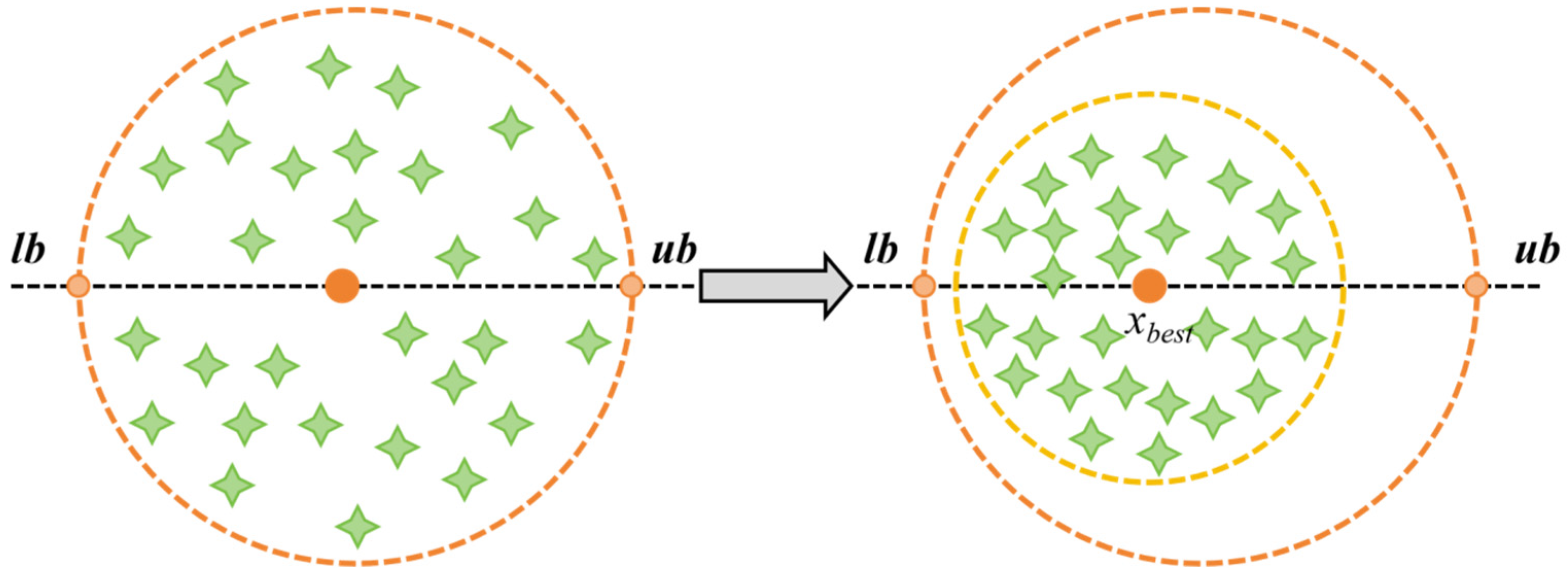
From a holistic coordination perspective, the leader-guided boundary control strategy demonstrates strong complementarity with the two aforementioned improvement strategies. The elite pool-enhanced exploration strategy primarily enhances multidirectional search capabilities within high-quality regions, while the stochastic centroid reverse learning strategy focuses on expanding the search space and improving the ability to escape local optima. The leader-guided boundary control strategy further implements targeted corrections for boundary-crossing individuals, strengthening local exploitation and stable convergence near the boundaries. Through their synergistic interaction, MEBBO achieves an optimal balance among exploration capability, exploitation capability, and boundary processing capability. The mechanism of the leader-guided boundary control strategy is illustrated in Figure 2, and the complete pseudocode of MEBBO is presented in Algorithm 1.

The following is the pseudocode of Algorithm 1.

Algorithm 1. MEBBO
Initialize population x and evaluate fitness	//Generate initial solutions and calculate fitness
Set $N_e$ = round(0.2N)	//Define the elite pool size
for t = 1 to T do
Compute E	//Calculate the dam-phase factor
Update elite pool EP with top $N_e$ individuals	//Preserve high-quality individuals
Divide top 25% individuals as architects	//Identify architect individuals
for each xi do	//Update each individual
if rand < E then
Update xi in exploitation phase	//Refine search around promising regions
else
if xi is architect then
Update xi by learning from a random elite individual	//Elite-guided exploration
else
Update xi by learning from architects or Gaussian disturbance	//Prospector search with stochastic perturbation
end if
end if
end for
Perform leader-guided boundary control	//Correct out-of-bound individuals
Evaluate xi and update xbest if necessary	//Update fitness and global best solution
end for
return xbest	//Output the best solution

3.3. Computational Complexity Analysis

The computational complexity of the proposed MEBBO is analyzed in comparison with the original BBO. Let (N), (D), (T), and (F) denote the population size, problem dimension, maximum number of iterations, and the computational cost of one objective function evaluation, respectively. For BBO, the population initialization requires (O(ND)), and each iteration mainly involves dimension-wise population updating, fitness-based ranking, and objective function evaluation. Therefore, the overall time complexity of BBO can be expressed as (O(ND + T(ND + NlogN + NF))). Compared with BBO, MEBBO introduces three additional mechanisms, including elite-pool enhanced exploration, random centroid-based reverse learning, and leader-guided boundary control. The elite-pool strategy relies on fitness-based ranking and does not change the asymptotic sorting complexity, while the leader-guided boundary control only introduces additional dimension-wise operations. The main extra computational cost of MEBBO comes from the random centroid-based reverse learning strategy, which generates reverse candidate solutions and performs additional objective function evaluations for greedy selection. Accordingly, the time complexity of MEBBO can be written as (O(ND + T(ND + NlogN + 3NF))). When the cost of objective function evaluation is approximately proportional to the problem dimension, both BBO and MEBBO have the same asymptotic time complexity of (O(TND)). However, MEBBO has a larger constant computational overhead due to the additional enhancement mechanisms. In terms of space complexity, both algorithms are dominated by the storage of population-related matrices, fitness vectors, and the best solution, resulting in a space complexity of (O(ND)). Therefore, the proposed MEBBO improves the search capability of BBO while maintaining the same asymptotic time and space complexity.

3.4. Time Comparison Analysis of BBO and MEBBO

Execution time analysis was further conducted to evaluate the computational cost of MEBBO compared with the original BBO. Under the same experimental settings, including a population size of 30, a maximum iteration number of 100, and 30 independent runs on the CEC2017 30D test suite, MEBBO requires more running time than BBO on all 30 benchmark functions. Specifically, the average execution time of BBO over all functions is 0.3267 s, whereas that of MEBBO is 0.9083 s, approximately 2.78 times that of BBO. This increase is mainly attributed to the additional computational operations introduced by the elite pool-enhanced exploration, stochastic centroid reverse learning, and leader-guided boundary control strategies. Nevertheless, the absolute running time of MEBBO remains within an acceptable range, with all average times below 2.2 s. Considering the significant improvements in solution accuracy, convergence behavior, and classification performance reported in the previous experiments, the additional computational cost of MEBBO is acceptable and reflects a reasonable trade-off between optimization performance and running efficiency. The execution time comparison is reported in

Table 2. Execution time comparison between BBO and MEBBO on CEC2017 (30D).

Algorithm	F1	F2	F3	F4	F5	F6
BBO	2.2178 × 10−1	2.4956 × 10−1	2.1768 × 10−1	2.2673 × 10−1	2.7380 × 10−1	2.9620 × 10−1
MEBBO	5.7972 × 10−1	6.1839 × 10−1	5.6409 × 10−1	5.9144 × 10−1	6.4397 × 10−1	9.0659 × 10−1
Algorithm	F7	F8	F9	F10	F11	F12
BBO	2.3575 × 10−1	2.6136 × 10−1	2.4851 × 10−1	2.5866 × 10−1	2.3883 × 10−1	2.6355 × 10−1
MEBBO	6.8647 × 10−1	6.5326 × 10−1	6.6722 × 10−1	7.2123 × 10−1	6.0864 × 10−1	6.5314 × 10−1
Algorithm	F13	F14	F15	F16	F17	F18
BBO	2.3882 × 10−1	2.7553 × 10−1	2.3164 × 10−1	2.4170 × 10−1	3.0761 × 10−1	2.4281 × 10−1
MEBBO	6.2758 × 10−1	6.9960 × 10−1	6.1110 × 10−1	6.6880 × 10−1	8.1123 × 10−1	6.5435 × 10−1
Algorithm	F19	F20	F21	F22	F23	F24
BBO	5.2436 × 10−1	3.4339 × 10−1	3.7394 × 10−1	3.5144 × 10−1	4.0224 × 10−1	4.0871 × 10−1
MEBBO	1.5539 × 100	8.4379 × 10−1	9.2328 × 10−1	9.9755 × 10−1	1.0682 × 100	1.1353 × 100
Algorithm	F25	F26	F27	F28	F29	F30
BBO	2.7806 × 10−1	4.5682 × 10−1	5.7676 × 10−1	4.6014 × 10−1	3.7500 × 10−1	7.1910 × 10−1
MEBBO	7.8492 × 10−1	1.3930 × 100	1.7625 × 100	1.4352 × 100	1.2125 × 100	2.1735 × 100

.

4. Numerical Experiments

This section primarily investigates the convergence characteristics of the MEBBO algorithm and conducts a systematic performance comparison with 9 other optimization algorithms using two benchmark test suites: CEC2017 and CEC2022. The CEC2017 test suite was implemented across search spaces of 30, 50, and 100 dimensions, while the CEC2022 test suite was conducted under 10-dimensional and 20-dimensional conditions, totaling 42 test functions, as detailed in

Table 3. CEC 2017 benchmark functions.

Type	ID	Description	Dim	fmin
Unimodal	F1	Shifted and Rotated Bent Cigar Function	30/50/100	100
	F2	Shifted and Rotated Sum of Different Power Function	30/50/100	200
	F3	Shifted and Rotated Zakharov Function	30/50/100	300
Multimodal	F4	Shifted and Rotated Rosenbrock’s Function	30/50/100	400
	F5	Shifted and Rotated Rastrigin’s Function	30/50/100	500
	F6	Shifted and Rotated Expanded Scaffer’s F6 Function	30/50/100	600
	F7	Shifted and Rotated Lunacek Bi_Rastrigin Function	30/50/100	700
	F8	Shifted and Rotated Non-Continuous Rastrigin’s Function	30/50/100	800
	F9	Shifted and Rotated Levy Function	30/50/100	900
	F10	Shifted and Rotated Schwefel’s Function	30/50/100	1000
Hybrid	F11	Hybrid Function 1 (N = 3)	30/50/100	1100
	F12	Hybrid Function 2 (N = 3)	30/50/100	1200
	F13	Hybrid Function 3 (N = 3)	30/50/100	1300
	F14	Hybrid Function 6 (N = 4)	30/50/100	1400
	F15	Hybrid Function 6 (N = 4)	30/50/100	1500
	F16	Hybrid Function 6 (N = 4)	30/50/100	1600
	F17	Hybrid Function 6 (N = 5)	30/50/100	1700
	F18	Hybrid Function 6 (N = 5)	30/50/100	1800
	F19	Hybrid Function 6 (N = 5)	30/50/100	1900
	F20	Hybrid Function 6 (N = 6)	30/50/100	2000
Composition	F21	Composition Function 1 (N = 5)	30/50/100	2100
	F22	Composition Function 2 (N = 5)	30/50/100	2200
	F23	Composition Function 3 (N = 5)	30/50/100	2300
	F24	Composition Function 4 (N = 5)	30/50/100	2400
	F25	Composition Function 5 (N = 3)	30/50/100	2500
	F26	Composition Function 6 (N = 3)	30/50/100	2600
	F27	Composition Function 7 (N = 5)	30/50/100	2700
	F28	Composition Function 8 (N = 5)	30/50/100	2800
	F29	Composition Function 9 (N =5)	30/50/100	2900
	F30	Composition Function 10 (N = 3)	30/50/100	3000
Search Range: [−100, 100]D

and

Table 4. CEC 2022 benchmark functions.

Type	ID	Description	Dim	fmin
Unimodal Function	F1	Shifted and full Rotated Zakharov Function	10/20	300
Basic Functions	F2	Shifted and full Rotated Zakharov Function	10/20	400
	F3	Shifted and full Rotated Expanded Schaffer’s f6 Function	10/20	600
	F4	Shifted and full Rotated Non-Continuous Rastrigin’s Function	10/20	800
	F5	Shifted and full Rotated Levy Function	10/20	900
Hybrid Functions	F6	Hybrid Function 1 (N = 3)	10/20	1800
	F7	Hybrid Function 2 (N =6)	10/20	2000
	F8	Hybrid Function 3 (N = 5)	10/20	2200
Composition Functions	F9	Composition Function 1 (N = 5)	10/20	2300
	F10	Composition Function 2 (N = 4)	10/20	2400
	F11	Composition Function 3 (N = 5)	10/20	2600
	F12	Composition Function 4 (N = 6)	10/20	2700
Search Range: [−100, 100]D

. To minimize the impact of randomness on experimental results, each algorithm was executed multiple times independently, with the mean and standard deviation of optimization outcomes statistically analyzed to comprehensively evaluate solution accuracy and stability.

To enhance the statistical reliability of the experimental conclusions, this study employs two non-parametric statistical methods—the Wilcoxon rank-sum test and the Friedman test—to analyze performance differences and the overall ranking of the algorithms. Specifically, in the Wilcoxon rank-sum test, a p-value below 0.05 indicates a significant difference between the comparison algorithm and MEBBO, while a p-value above 0.05 suggests no statistically significant difference. The notation “+/=/−” is used to denote whether MEBBO outperforms, performs comparably to, or underperforms the comparison algorithm. For the Friedman test, the average rank of each algorithm across all test functions is first calculated, and the algorithms are then ranked according to determine whether statistically significant differences exist among them.

4.1. CEC2017 and CEC2022 Test Suite

The aforementioned test functions can be categorized into different types based on their properties and testing objectives. Unimodal functions contain only one global optimum and are primarily used to evaluate algorithm convergence speed and solution accuracy. Multimodal functions include multiple local optima and mainly serve to assess the algorithm’s ability to escape local optima and its robustness. Hybrid and composite functions integrate the characteristics of the first two categories, enabling more effective simulation of complex optimization problems and further evaluating the algorithms’ global optimization capabilities and overall performance in challenging search environments. All experiments were conducted on a computer equipped with an Intel Core i5-1135G7 2.40 GHz processor and 16 GB RAM, using the MATLAB 2021a platform. To ensure a fair comparison among algorithms, all numerical experiments in this section uniformly set the maximum number of iterations to 500 and the population size to 30.

4.2. Algorithm Parameter Settings

Table 5. Parameters setting for different algorithms.

Algorithms	Name of the Parameter	Value of the Parameter
EWOA [39]	$a,b$	$a\mathrm{l}\mathrm{i}\mathrm{n}\mathrm{e}\mathrm{a}\mathrm{r}\mathrm{l}\mathrm{y}\mathrm{d}\mathrm{e}\mathrm{c}\mathrm{r}\mathrm{e}\mathrm{a}\mathrm{s}\mathrm{e}\mathrm{s}\mathrm{f}\mathrm{r}\mathrm{o}\mathrm{m}2\mathrm{t}\mathrm{o}0;b=1$
PHHO [40]	$E_0$	[−1, 1]
MELGWO [41]	$P_{min},a,C_1$	10; linearly decreases from 2 to 0; 2
TACPSO [42]	$w_{max},w_{min},c_{1i},c_{1f},c_{2i},c_{2f}$	0.9, 0.4, 2.5, 0.5, 0.5, 2.5
CFOA [43]	rs	[−1, 1]
ALA [44]	F	[−1, 1]
AOO [45]	c	[0, 1]
RIME [46]	$w$	5
BBO [20]	E	[0, 1]
MEBBO	$a,$ ${\mathrm{E}}_{\mathrm{p}}$, Ne	[0, 2]; 3; 0.2

presents the parameter settings for MEBBO and the comparative algorithms. The comparative algorithms include the Enhanced Whale Optimization Algorithm (EWOA), Hybrid Parallel Harris Hawks Optimization (HPHHO), Improved Grey Wolf Optimizer with Memory Mechanism, Evolutionary Operator, and Local Search (MELGWO), Time-Varying Acceleration Particle Swarm Optimization (TACPSO), Catch Fish Optimization Algorithm (CFOA), Artificial Lemming Algorithm (ALA), Animated Oat Optimization Algorithm (AOO), RIME Optimization Algorithm (RIME), and the BBO.

4.3. Convergence Behavior Evaluation

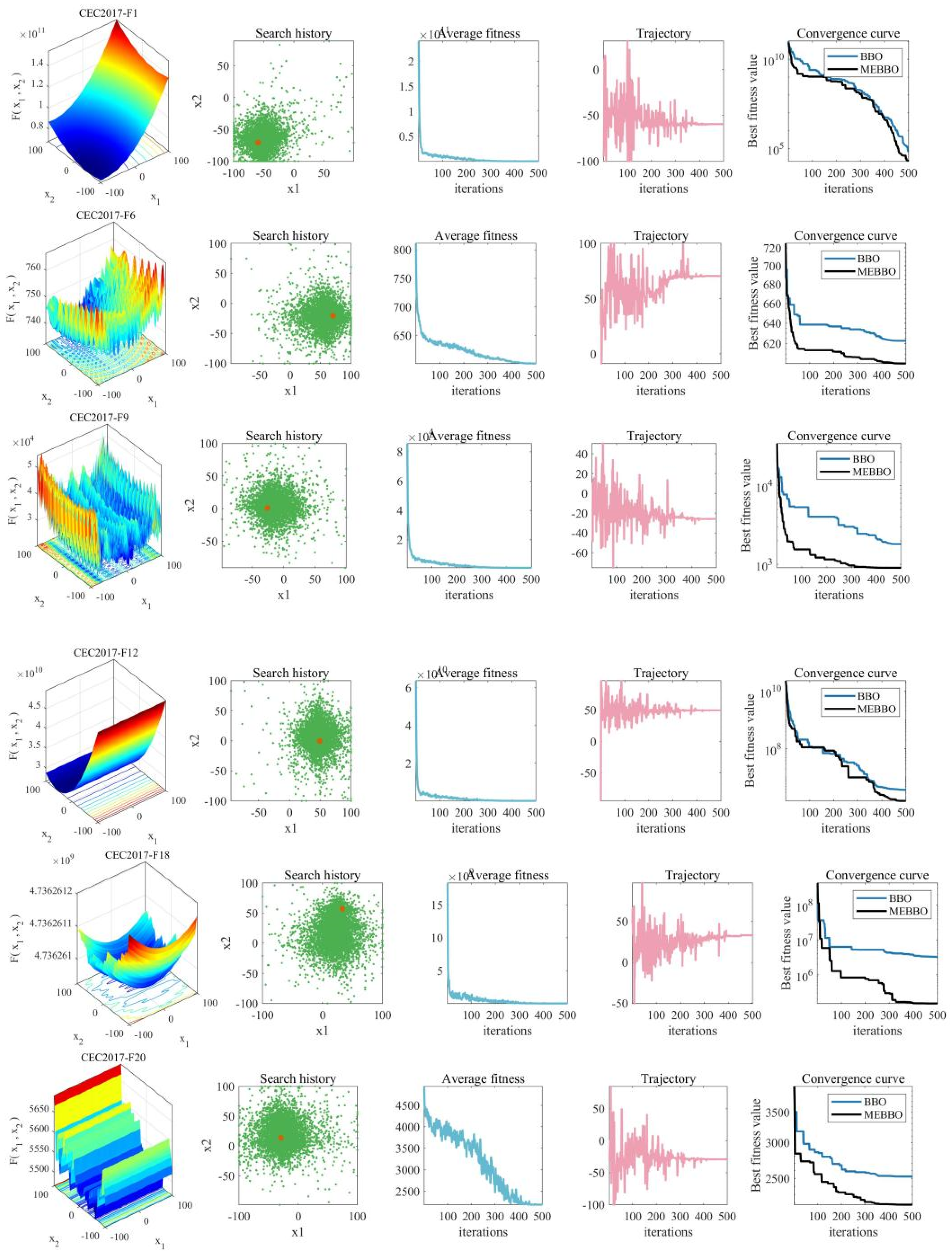
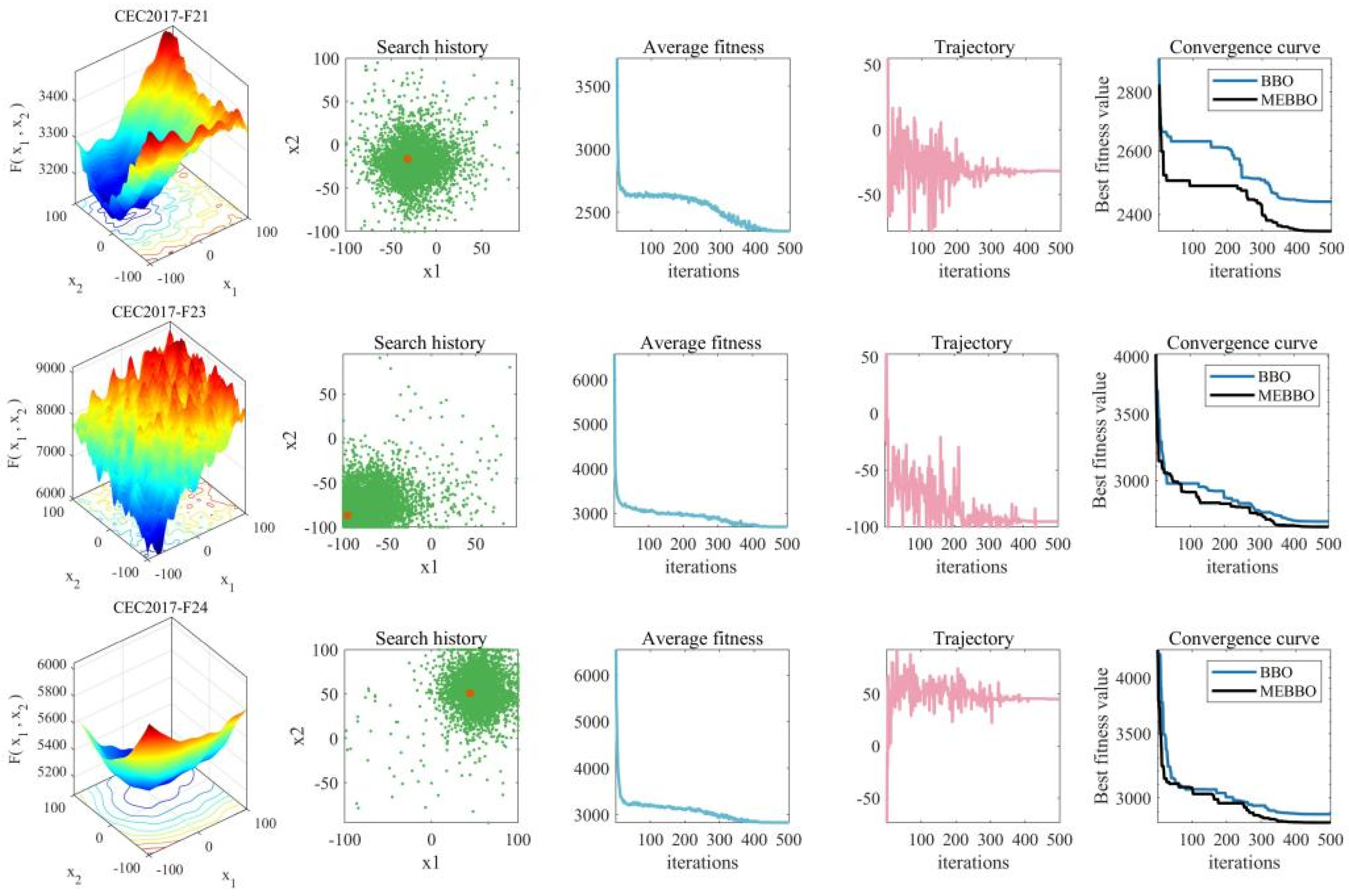
To validate the effectiveness of the proposed MEBBO algorithm, this study further presents convergence plots for various benchmark functions and analyzes its optimization process from multiple perspectives, including search distribution, fitness evolution, individual trajectory changes, and convergence curves. As shown in Figure 3, although the search individuals initially exhibit dispersed distributions across the test functions, the population gradually converges toward the neighborhoods of the optimal solutions during the iterations, with most individuals ultimately clustering near the global optimum regions. This demonstrates that MEBBO maintains strong global exploration capabilities while effectively exploiting advantageous regions, showcasing an excellent balance between exploration and exploitation. The average fitness curve initially shows a rapid decline followed by gradual stabilization, indicating that the multi-strategy enhancement mechanism significantly improves early-stage search efficiency while ensuring stable convergence in later iterations. Analysis of individual trajectories in one-dimensional space reveals that MEBBO maintains pronounced positional fluctuations during the initial iterations, reflecting robust population activity and the ability to escape local optima. In the later stages, these fluctuations diminish as the search trajectories become more concentrated, demonstrating the algorithm’s capability to progressively identify potentially optimal regions and achieve stable approximation. Finally, analysis of the overall convergence trajectories reveals distinct patterns. For unimodal functions, MEBBO demonstrates smooth convergence curves, indicating the algorithm’s ability to steadily approach optimal values through continuous iterations. In contrast, multimodal, hybrid, and composite functions exhibit staged or stepwise descent characteristics, demonstrating the algorithm’s capability to escape local optima and progressively converge toward global optimality in complex search environments. The convergence results conclusively show that MEBBO not only inherits the robust global search framework of the original BBO but also enhances population diversity, convergence speed, and global optimization performance through the synergy of multiple strategies, including elite pool-enhanced exploration, stochastic centroid reverse learning, and leader-guided boundary control. These improvements enable MEBBO to achieve superior convergence performance and search stability in complex optimization problems.

4.4. Comparison with Other Competitive Algorithms on CEC 2017

This section evaluates the performance of the proposed MEBBO algorithm against other benchmark algorithms using the CEC 2017 test suite across three dimensional scenarios: 30-dimensional, 50-dimensional, and 100-dimensional.

Table 6. Experimental results of 10 algorithms on the CEC 2017 (Dim = 30).

Algorithm	Metric	EWOA	HPHHO	MELGWO	TACPSO	CFOA	ALA	AOO	RIME	BBO	MEBBO
F1	Mean	2.2693 × 107	2.3339 × 109	1.9227 × 109	1.9341 × 108	5.0604 × 108	3.2298 × 106	1.1583 × 106	3.7040 × 106	1.1294 × 105	6.7147 × 104
	Std	3.6837 × 107	1.2168 × 109	1.5582 × 109	5.0915 × 108	2.1687 × 108	2.7629 × 106	6.2190 × 105	1.4258 × 106	9.0397 × 104	5.9676 × 104
F2	Mean	2.0958 × 1024	1.0000 × 1020	8.8795 × 1032	9.7958 × 1029	8.7814 × 1025	1.8607 × 1024	2.6639 × 1020	4.8418 × 1017	4.2545 × 1014	6.4660 × 1012
	Std	8.5421 × 1024	0.0000 × 100	4.8635 × 1033	5.3564 × 1030	2.3545 × 1026	7.0336 × 1024	1.1777 × 1021	1.8058 × 1018	1.5915 × 1015	1.4397 × 1013
F3	Mean	1.0604 × 105	4.6820 × 104	4.1854 × 104	4.8065 × 104	5.8472 × 104	2.8482 × 104	4.0797 × 104	4.7821 × 104	1.8413 × 104	1.5578 × 104
	Std	2.3184 × 104	7.6996 × 103	1.2090 × 104	1.4696 × 104	1.3261 × 104	7.5602 × 103	1.0915 × 104	1.9626 × 104	1.0141 × 104	6.8888 × 103
F4	Mean	5.3396 × 102	7.4901 × 102	6.4718 × 102	5.0987 × 102	6.4440 × 102	5.3493 × 102	5.1875 × 102	5.2042 × 102	5.0201 × 102	4.9972 × 102
	Std	3.4168 × 101	1.2338 × 102	1.5849 × 102	2.5358 × 101	5.4858 × 101	3.4010 × 101	2.3389 × 101	3.1209 × 101	2.3120 × 101	2.0025 × 101
F5	Mean	6.7077 × 102	7.7783 × 102	6.7779 × 102	6.0123 × 102	6.6302 × 102	6.1224 × 102	6.2562 × 102	6.1577 × 102	5.9267 × 102	5.4951 × 102
	Std	4.5836 × 101	3.3986 × 101	4.2819 × 101	3.2140 × 101	1.6892 × 101	2.7062 × 101	3.0647 × 101	3.0266 × 101	2.5491 × 101	1.6141 × 101
F6	Mean	6.3324 × 102	6.5969 × 102	6.4162 × 102	6.1166 × 102	6.3165 × 102	6.1318 × 102	6.3045 × 102	6.1483 × 102	6.1558 × 102	6.0266 × 102
	Std	1.1542 × 101	9.5220 × 100	8.0211 × 100	5.8915 × 100	7.4192 × 100	7.6515 × 100	7.3087 × 100	5.8483 × 100	7.3072 × 100	1.7100 × 100
F7	Mean	9.7700 × 102	1.2537 × 103	9.9506 × 102	8.5922 × 102	9.8644 × 102	9.0004 × 102	8.9618 × 102	8.5932 × 102	8.6567 × 102	7.9205 × 102
	Std	5.7329 × 101	9.4710 × 101	6.1485 × 101	3.9294 × 101	4.8256 × 101	3.4578 × 101	4.8890 × 101	2.5966 × 101	3.5043 × 101	2.2189 × 101
F8	Mean	9.5243 × 102	1.0008 × 103	9.3893 × 102	8.9602 × 102	9.4820 × 102	9.1036 × 102	9.1136 × 102	9.1344 × 102	8.7985 × 102	8.3884 × 102
	Std	3.9975 × 101	3.1405 × 101	2.5138 × 101	2.7059 × 101	2.3664 × 101	3.0927 × 101	1.9683 × 101	2.8323 × 101	1.7653 × 101	1.0247 × 101
F9	Mean	4.8664 × 103	6.6128 × 103	4.0207 × 103	2.1228 × 103	2.4421 × 103	2.1193 × 103	3.6970 × 103	2.9172 × 103	2.1513 × 103	9.2977 × 102
	Std	2.5778 × 103	6.8807 × 102	8.2601 × 102	7.5757 × 102	7.9933 × 102	1.4521 × 103	1.6921 × 103	1.4865 × 103	7.6001 × 102	2.7533 × 101
F10	Mean	6.1707 × 103	6.3264 × 103	5.4459 × 103	5.0592 × 103	6.6134 × 103	6.0525 × 103	4.7569 × 103	4.7039 × 103	4.4743 × 103	4.0368 × 103
	Std	1.2558 × 103	6.8411 × 102	7.2502 × 102	8.5616 × 102	6.4362 × 102	1.0495 × 103	7.5277 × 102	7.2255 × 102	7.6973 × 102	5.9631 × 102
F11	Mean	1.4521 × 103	1.6545 × 103	1.6715 × 103	1.2926 × 103	1.5508 × 103	1.2824 × 103	1.3013 × 103	1.3481 × 103	1.2491 × 103	1.2483 × 103
	Std	2.1927 × 102	1.9733 × 102	5.8767 × 102	7.3014 × 101	1.4208 × 102	5.5798 × 101	5.3252 × 101	5.9319 × 101	3.7066 × 101	4.2830 × 101
F12	Mean	3.2588 × 106	1.4542 × 108	4.2541 × 107	2.0315 × 106	3.6185 × 107	3.2042 × 106	1.6463 × 107	2.0315 × 107	3.7436 × 106	1.5322 × 106
	Std	2.2908 × 106	8.5627 × 107	4.7374 × 107	3.5889 × 106	2.1165 × 107	2.7631 × 106	1.3457 × 107	1.9627 × 107	2.9261 × 106	1.1102 × 106
F13	Mean	1.7009 × 104	4.3614 × 106	2.2290 × 105	1.7139 × 105	3.5484 × 104	4.0201 × 104	1.3315 × 105	2.8122 × 105	5.1690 × 104	3.6830 × 104
	Std	1.7316 × 104	1.1218 × 107	6.8863 × 105	8.0815 × 105	1.5840 × 104	2.5536 × 104	1.4501 × 105	5.2825 × 105	2.8241 × 104	1.5051 × 104
F14	Mean	2.7135 × 105	5.3120 × 105	1.9369 × 105	3.1130 × 104	1.5226 × 104	1.9782 × 103	9.1227 × 104	8.6622 × 104	3.6769 × 104	1.7780 × 104
	Std	2.5305 × 105	6.1397 × 105	2.0128 × 105	3.1566 × 104	1.2422 × 104	6.0805 × 102	6.8576 × 104	9.1474 × 104	2.9306 × 104	1.4810 × 104
F15	Mean	1.1886 × 104	7.2794 × 104	2.5642 × 104	7.0279 × 103	2.8344 × 104	2.3994 × 104	5.8177 × 104	1.8135 × 104	2.0110 × 104	2.0545 × 104
	Std	8.8010 × 103	5.9374 × 104	2.0451 × 104	8.4744 × 103	1.7082 × 104	1.3703 × 104	4.3717 × 104	1.1953 × 104	1.1669 × 104	1.2312 × 104
F16	Mean	2.7610 × 103	3.2357 × 103	2.9082 × 103	2.6016 × 103	2.7749 × 103	2.7626 × 103	2.7388 × 103	2.6732 × 103	2.6131 × 103	2.4721 × 103
	Std	3.4768 × 102	3.8325 × 102	2.8582 × 102	2.4796 × 102	2.5758 × 102	3.5988 × 102	3.0985 × 102	2.9691 × 102	3.2166 × 102	2.7188 × 102
F17	Mean	2.3709 × 103	2.3042 × 103	2.2815 × 103	2.2170 × 103	2.0209 × 103	2.1388 × 103	2.2034 × 103	2.1902 × 103	2.1027 × 103	1.9426 × 103
	Std	2.9998 × 102	2.1544 × 102	2.9869 × 102	1.7712 × 102	1.0049 × 102	1.7790 × 102	1.8280 × 102	1.8674 × 102	1.4068 × 102	1.2734 × 102
F18	Mean	2.1304 × 106	2.7481 × 106	8.9078 × 105	3.2235 × 105	1.8430 × 105	8.4939 × 104	1.0986 × 106	1.5614 × 106	6.3169 × 105	5.7498 × 105
	Std	2.6979 × 106	3.2206 × 106	8.5804 × 105	3.0075 × 105	1.5003 × 105	6.3796 × 104	1.5735 × 106	1.2505 × 106	6.3435 × 105	7.0389 × 105
F19	Mean	9.4894 × 103	2.0467 × 106	3.6578 × 104	1.0456 × 104	1.7422 × 105	2.4583 × 104	5.3671 × 105	1.4940 × 104	1.3609 × 104	2.0168 × 104
	Std	8.1969 × 103	2.9158 × 106	4.6668 × 104	2.5584 × 104	3.1799 × 105	2.1119 × 104	4.8371 × 105	1.0705 × 104	7.4197 × 103	1.8257 × 104
F20	Mean	2.6678 × 103	2.5908 × 103	2.6141 × 103	2.5210 × 103	2.4247 × 103	2.5456 × 103	2.5961 × 103	2.5009 × 103	2.4055 × 103	2.3384 × 103
	Std	1.7738 × 102	2.1805 × 102	1.8873 × 102	1.7424 × 102	9.3416 × 101	1.7631 × 102	2.0956 × 102	2.4275 × 102	1.5272 × 102	1.1550 × 102
F21	Mean	2.4357 × 103	2.5488 × 103	2.4551 × 103	2.3937 × 103	2.4405 × 103	2.4092 × 103	2.4228 × 103	2.4176 × 103	2.3839 × 103	2.3508 × 103
	Std	3.4231 × 101	4.2932 × 101	3.9815 × 101	2.4875 × 101	1.9921 × 101	2.5983 × 101	3.6827 × 101	2.7773 × 101	2.8678 × 101	1.2247 × 101
F22	Mean	2.3267 × 103	5.0533 × 103	5.6562 × 103	4.2158 × 103	2.6712 × 103	6.4065 × 103	5.9041 × 103	4.9702 × 103	3.2155 × 103	2.3023 × 103
	Std	1.4975 × 101	2.2068 × 103	1.7709 × 103	1.9164 × 103	9.9301 × 102	2.3885 × 103	1.6076 × 103	1.8347 × 103	1.7049 × 103	1.3460 × 100
F23	Mean	2.8260 × 103	2.9798 × 103	2.8360 × 103	2.7766 × 103	2.8253 × 103	2.7825 × 103	2.8066 × 103	2.7872 × 103	2.7508 × 103	2.7199 × 103
	Std	7.0147 × 101	9.0738 × 101	6.2194 × 101	4.0689 × 101	3.9328 × 101	3.8588 × 101	3.6433 × 101	3.6593 × 101	3.4250 × 101	1.9430 × 101
F24	Mean	2.9966 × 103	3.1949 × 103	2.9824 × 103	2.9864 × 103	2.9786 × 103	2.9601 × 103	2.9799 × 103	2.9439 × 103	2.9131 × 103	2.8634 × 103
	Std	5.3225 × 101	7.2225 × 101	4.6772 × 101	7.3380 × 101	3.3162 × 101	3.9739 × 101	5.2945 × 101	3.5505 × 101	3.2792 × 101	2.0014 × 101
F25	Mean	2.9270 × 103	3.0821 × 103	3.0059 × 103	2.9091 × 103	3.0372 × 103	2.9153 × 103	2.9214 × 103	2.9318 × 103	2.8997 × 103	2.9004 × 103
	Std	2.6990 × 101	6.3146 × 101	5.0330 × 101	2.1922 × 101	4.0013 × 101	1.6109 × 101	2.1738 × 101	2.6592 × 101	1.6100 × 101	1.6753 × 101
F26	Mean	5.5405 × 103	6.9566 × 103	6.0540 × 103	4.2857 × 103	5.0205 × 103	5.0304 × 103	4.5901 × 103	5.0879 × 103	4.6633 × 103	3.6451 × 103
	Std	9.0190 × 102	1.3973 × 103	5.9397 × 102	1.0769 × 103	1.2808 × 103	3.6687 × 102	9.5594 × 102	6.4269 × 102	1.0953 × 103	7.3927 × 102
F27	Mean	3.2731 × 103	3.3776 × 103	3.2977 × 103	3.2687 × 103	3.2694 × 103	3.2391 × 103	3.2861 × 103	3.2470 × 103	3.2370 × 103	3.2417 × 103
	Std	3.6044 × 101	9.0997 × 101	4.1306 × 101	3.3592 × 101	2.7184 × 101	1.8338 × 101	3.5386 × 101	2.0529 × 101	1.5517 × 101	1.5187 × 101
F28	Mean	3.2825 × 103	3.4635 × 103	3.4625 × 103	3.2644 × 103	3.4088 × 103	3.8315 × 103	3.2856 × 103	3.2966 × 103	3.2320 × 103	3.2185 × 103
	Std	2.3283 × 101	7.8438 × 101	1.2287 × 102	2.7525 × 101	5.8347 × 101	1.2151 × 103	4.0350 × 101	3.0885 × 101	2.1691 × 101	1.9718 × 101
F29	Mean	4.1037 × 103	4.4474 × 103	4.3483 × 103	3.8712 × 103	4.0576 × 103	4.0160 × 103	4.0094 × 103	4.0301 × 103	3.8401 × 103	3.6313 × 103
	Std	2.5728 × 102	3.1728 × 102	3.3225 × 102	2.2892 × 102	1.6819 × 102	2.0078 × 102	2.7371 × 102	2.4745 × 102	1.9641 × 102	1.3966 × 102
F30	Mean	2.3859 × 104	1.1552 × 107	2.7169 × 106	8.2189 × 104	2.6887 × 106	1.0650 × 105	4.1614 × 106	8.2258 × 105	2.4436 × 105	2.5353 × 105
	Std	1.3455 × 104	9.2151 × 106	2.2811 × 106	2.5875 × 105	2.3262 × 106	1.7525 × 105	2.5657 × 106	5.2299 × 105	2.1059 × 105	2.2369 × 105

,

Table 7. Experimental results of 10 algorithms on the CEC 2017 (Dim = 50).

Algorithm	Metric	EWOA	HPHHO	MELGWO	TACPSO	CFOA	ALA	AOO	RIME	BBO	MEBBO
F1	Mean	1.0130 × 109	2.0317 × 1010	1.3053 × 1010	6.4429 × 108	7.9186 × 109	6.5530 × 108	1.0734 × 108	3.9271 × 107	2.7950 × 106	8.4828 × 105
	Std	5.0337 × 108	3.5495 × 109	4.7142 × 109	8.9372 × 108	1.9823 × 109	3.7737 × 108	8.5732 × 107	1.3348 × 107	1.2516 × 106	5.5890 × 105
F2	Mean	1.0954 × 1060	1.0000 × 1020	2.3900 × 1053	9.8344 × 1051	4.6612 × 1056	3.1526 × 1053	2.6536 × 1048	6.5508 × 1040	1.8617 × 1034	5.2135 × 1027
	Std	5.9991 × 1060	0.0000 × 100	1.0173 × 1054	4.2490 × 1052	2.3466 × 1057	1.6814 × 1054	1.4465 × 1049	2.1369 × 1041	7.2634 × 1034	1.3338 × 1028
F3	Mean	2.5347 × 105	1.2386 × 105	1.3021 × 105	1.8092 × 105	1.5071 × 105	1.1546 × 105	1.6360 × 105	2.0779 × 105	1.2270 × 105	9.5138 × 104
	Std	4.1631 × 104	1.5941 × 104	1.7715 × 104	3.9998 × 104	2.5567 × 104	2.0269 × 104	3.6877 × 104	4.5245 × 104	2.6693 × 104	2.1377 × 104
F4	Mean	8.4001 × 102	2.7105 × 103	2.3346 × 103	7.0122 × 102	1.6864 × 103	7.6039 × 102	7.0067 × 102	6.8178 × 102	6.0086 × 102	6.0300 × 102
	Std	1.5020 × 102	8.3847 × 102	1.3234 × 103	9.2786 × 101	4.1819 × 102	9.3242 × 101	4.8452 × 101	5.9551 × 101	4.5512 × 101	4.7432 × 101
F5	Mean	8.6287 × 102	9.8861 × 102	8.3883 × 102	7.6007 × 102	8.9227 × 102	7.9029 × 102	7.6413 × 102	7.5819 × 102	6.9790 × 102	6.0849 × 102
	Std	7.8690 × 101	3.1869 × 101	3.8828 × 101	6.2833 × 101	3.0255 × 101	7.1440 × 101	4.7404 × 101	4.2749 × 101	3.7428 × 101	2.8867 × 101
F6	Mean	6.4572 × 102	6.7557 × 102	6.6140 × 102	6.2646 × 102	6.5286 × 102	6.2995 × 102	6.4901 × 102	6.3042 × 102	6.3092 × 102	6.0699 × 102
	Std	9.3337 × 100	5.1630 × 100	6.7617 × 100	8.9166 × 100	7.1877 × 100	6.6650 × 100	1.0436 × 101	8.6257 × 100	6.7991 × 100	2.4322 × 100
F7	Mean	1.4379 × 103	1.7952 × 103	1.4665 × 103	1.1094 × 103	1.4042 × 103	1.1864 × 103	1.1671 × 103	1.1560 × 103	1.0732 × 103	8.9127 × 102
	Std	1.5684 × 102	8.8375 × 101	1.1456 × 102	8.4177 × 101	8.4723 × 101	1.0017 × 102	5.3822 × 101	7.2713 × 101	5.4918 × 101	3.1944 × 101
F8	Mean	1.1428 × 103	1.2826 × 103	1.1410 × 103	1.0457 × 103	1.1970 × 103	1.0757 × 103	1.0680 × 103	1.0709 × 103	1.0075 × 103	8.9966 × 102
	Std	6.6011 × 101	3.6943 × 101	6.2167 × 101	4.1871 × 101	5.1435 × 101	6.2917 × 101	3.5845 × 101	5.6305 × 101	3.7494 × 101	2.1947 × 101
F9	Mean	2.0043 × 104	2.1951 × 104	1.2630 × 104	8.7726 × 103	1.3440 × 104	9.6627 × 103	1.3944 × 104	1.1345 × 104	7.1495 × 103	1.3271 × 103
	Std	7.0527 × 103	4.1965 × 103	2.1240 × 103	5.9152 × 103	3.5488 × 103	4.4853 × 103	3.9910 × 103	5.2482 × 103	1.8609 × 103	4.8931 × 102
F10	Mean	1.1050 × 104	1.0837 × 104	8.5493 × 103	8.6155 × 103	1.2595 × 104	1.1309 × 104	8.2838 × 103	7.6774 × 103	7.0790 × 103	6.4563 × 103
	Std	1.9599 × 103	8.9587 × 102	9.1432 × 102	1.0386 × 103	8.3640 × 102	1.6059 × 103	6.5166 × 102	9.5123 × 102	1.2561 × 103	8.4129 × 102
F11	Mean	3.3974 × 103	3.2939 × 103	3.8824 × 103	1.7236 × 103	6.6525 × 103	1.8001 × 103	1.7826 × 103	1.7604 × 103	1.4289 × 103	1.3844 × 103
	Std	1.2865 × 103	6.3858 × 102	1.6208 × 103	2.2321 × 102	1.6610 × 103	1.9391 × 102	2.2589 × 102	1.3534 × 102	7.3165 × 101	6.0947 × 101
F12	Mean	5.4513 × 107	1.9442 × 109	1.0853 × 109	3.3392 × 108	3.8737 × 108	3.4371 × 107	1.4356 × 108	1.5802 × 108	2.0926 × 107	1.6014 × 107
	Std	4.1320 × 107	1.1022 × 109	1.2517 × 109	9.7288 × 108	1.7722 × 108	1.9149 × 107	8.9953 × 107	9.9366 × 107	1.5177 × 107	8.4877 × 106
F13	Mean	3.3632 × 104	1.2947 × 108	3.8442 × 107	4.7533 × 107	8.1947 × 105	4.2106 × 105	1.2308 × 105	4.8638 × 105	7.8753 × 104	6.9002 × 104
	Std	2.2168 × 104	1.0348 × 108	6.5533 × 107	1.5402 × 108	8.5287 × 105	1.9822 × 106	8.0352 × 104	2.9127 × 105	3.3983 × 104	2.6912 × 104
F14	Mean	1.6445 × 106	2.1299 × 106	9.9340 × 105	3.1789 × 105	1.6859 × 105	9.5268 × 104	8.3226 × 105	7.9483 × 105	3.9143 × 105	1.5378 × 105
	Std	1.3724 × 106	2.0132 × 106	1.1045 × 106	2.4237 × 105	1.8694 × 105	2.0374 × 105	6.5542 × 105	5.0518 × 105	3.9732 × 105	8.9133 × 104
F15	Mean	1.1717 × 104	1.1324 × 107	3.0799 × 106	1.1667 × 104	2.1871 × 104	2.5807 × 104	4.9172 × 104	1.0854 × 105	2.9791 × 104	2.5866 × 104
	Std	6.4479 × 103	1.4558 × 107	1.3540 × 107	8.6151 × 103	8.5146 × 103	1.8823 × 104	2.4263 × 104	3.5756 × 104	1.4002 × 104	1.1664 × 104
F16	Mean	3.7879 × 103	4.8846 × 103	3.9132 × 103	3.3134 × 103	3.6793 × 103	3.8202 × 103	3.6065 × 103	3.9087 × 103	3.1810 × 103	2.8879 × 103
	Std	4.0265 × 102	6.2720 × 102	4.9439 × 102	3.9901 × 102	3.5014 × 102	5.2241 × 102	5.4673 × 102	4.6382 × 102	3.3192 × 102	3.4966 × 102
F17	Mean	3.5414 × 103	3.7079 × 103	3.5066 × 103	3.1803 × 103	3.1651 × 103	3.6191 × 103	3.0975 × 103	3.4545 × 103	3.0612 × 103	2.9383 × 103
	Std	3.9428 × 102	3.9295 × 102	3.4110 × 102	3.6243 × 102	2.4793 × 102	3.5102 × 102	2.5187 × 102	4.1300 × 102	2.9067 × 102	3.2023 × 102
F18	Mean	4.4115 × 106	8.3596 × 106	6.8810 × 106	1.3956 × 106	2.1283 × 106	9.3241 × 105	4.0292 × 106	5.1905 × 106	2.1207 × 106	2.0014 × 106
	Std	3.7474 × 106	8.1510 × 106	7.8042 × 106	8.8533 × 105	1.7657 × 106	9.1683 × 105	2.3118 × 106	3.9610 × 106	1.5443 × 106	1.0184 × 106
F19	Mean	1.3285 × 104	2.6947 × 106	6.3015 × 105	2.0391 × 104	5.5104 × 105	1.5871 × 104	1.1108 × 106	6.0653 × 105	7.1223 × 104	1.0945 × 105
	Std	1.1736 × 104	2.3349 × 106	1.4229 × 106	1.4030 × 104	5.0017 × 105	1.3331 × 104	8.4034 × 105	5.8656 × 105	5.4150 × 104	6.2906 × 104
F20	Mean	3.5088 × 103	3.3280 × 103	3.3207 × 103	3.4017 × 103	3.2629 × 103	3.5948 × 103	3.3090 × 103	3.3738 × 103	3.0806 × 103	2.7441 × 103
	Std	3.3853 × 102	2.5684 × 102	3.5219 × 102	3.2980 × 102	2.8514 × 102	2.6405 × 102	3.1318 × 102	3.8717 × 102	2.4156 × 102	3.9771 × 102
F21	Mean	2.6421 × 103	2.8794 × 103	2.6636 × 103	2.5215 × 103	2.6632 × 103	2.5759 × 103	2.5776 × 103	2.5582 × 103	2.4843 × 103	2.3965 × 103
	Std	6.9755 × 101	4.7949 × 101	6.7292 × 101	4.6595 × 101	3.8667 × 101	4.2203 × 101	5.0652 × 101	5.2710 × 101	3.5343 × 101	2.0928 × 101
F22	Mean	1.1976 × 104	1.2867 × 104	1.0599 × 104	1.0449 × 104	1.2948 × 104	1.3683 × 104	9.5951 × 103	9.8403 × 103	8.3327 × 103	6.0478 × 103
	Std	1.3970 × 103	1.1412 × 103	9.3716 × 102	9.9642 × 102	3.1981 × 103	1.4269 × 103	1.0885 × 103	8.3281 × 102	1.9439 × 103	2.9738 × 103
F23	Mean	3.1258 × 103	3.5485 × 103	3.1831 × 103	3.0464 × 103	3.1720 × 103	3.0417 × 103	3.1156 × 103	3.0548 × 103	2.9676 × 103	2.8709 × 103
	Std	7.4934 × 101	1.4471 × 102	8.3441 × 101	7.5083 × 101	6.6784 × 101	6.2657 × 101	7.7513 × 101	6.5400 × 101	5.1130 × 101	3.0146 × 101
F24	Mean	3.3087 × 103	3.7399 × 103	3.2828 × 103	3.3042 × 103	3.3285 × 103	3.2367 × 103	3.3101 × 103	3.1857 × 103	3.1048 × 103	3.0121 × 103
	Std	1.2808 × 102	1.4007 × 102	9.3015 × 101	1.4741 × 102	6.0367 × 101	7.2632 × 101	1.0343 × 102	7.1308 × 101	5.0612 × 101	3.5663 × 101
F25	Mean	3.3028 × 103	4.4303 × 103	4.1218 × 103	3.1678 × 103	4.1436 × 103	3.2378 × 103	3.1977 × 103	3.1532 × 103	3.0901 × 103	3.0948 × 103
	Std	1.1597 × 102	3.7158 × 102	5.6168 × 102	6.8532 × 101	3.0160 × 102	6.7158 × 101	5.5805 × 101	5.2241 × 101	3.0813 × 101	2.9815 × 101
F26	Mean	7.9029 × 103	1.2539 × 104	9.4662 × 103	7.4706 × 103	1.0253 × 104	7.2457 × 103	7.4634 × 103	7.4791 × 103	6.9264 × 103	5.3449 × 103
	Std	8.8235 × 102	1.6252 × 103	1.1227 × 103	2.2261 × 103	1.4366 × 103	6.7744 × 102	1.0550 × 103	9.9553 × 102	1.6968 × 103	1.0144 × 103
F27	Mean	3.6992 × 103	4.0558 × 103	3.8564 × 103	3.6572 × 103	3.8295 × 103	3.6040 × 103	3.7677 × 103	3.5861 × 103	3.4747 × 103	3.4660 × 103
	Std	1.5738 × 102	2.1698 × 102	2.0532 × 102	1.8442 × 102	1.5611 × 102	1.4596 × 102	1.2946 × 102	7.4973 × 101	8.5487 × 101	5.8087 × 101
F28	Mean	3.6865 × 103	5.4336 × 103	4.8359 × 103	3.5609 × 103	4.7940 × 103	5.1273 × 103	3.6342 × 103	3.4561 × 103	3.3662 × 103	3.3468 × 103
	Std	1.4545 × 102	3.7618 × 102	4.2250 × 102	1.4408 × 102	3.2628 × 102	2.3951 × 103	1.0796 × 102	4.7512 × 101	3.9251 × 101	3.6970 × 101
F29	Mean	4.7996 × 103	6.9081 × 103	6.0873 × 103	4.8999 × 103	5.5639 × 103	4.9872 × 103	5.1475 × 103	5.2231 × 103	4.6207 × 103	4.2579 × 103
	Std	4.5392 × 102	1.0119 × 103	5.2844 × 102	5.1766 × 102	4.5255 × 102	4.5207 × 102	4.4753 × 102	4.1111 × 102	3.3372 × 102	2.9926 × 102
F30	Mean	4.4022 × 106	2.2729 × 108	9.7754 × 107	2.0049 × 106	1.4246 × 108	4.1143 × 106	6.5758 × 107	5.7613 × 107	2.4273 × 107	2.5399 × 107
	Std	2.8007 × 106	9.8681 × 107	4.4191 × 107	1.2174 × 106	3.7743 × 107	2.7709 × 106	2.0437 × 107	2.3167 × 107	5.3287 × 106	4.7890 × 106

and

Table 8. Experimental results of 10 algorithms on the CEC 2017 (Dim = 100).

Algorithm	Metric	EWOA	HPHHO	MELGWO	TACPSO	CFOA	ALA	AOO	RIME	BBO	MEBBO
F1	Mean	2.2391 × 1010	9.8630 × 1010	7.7962 × 1010	1.4561 × 1010	6.8331 × 1010	2.2462 × 1010	1.0797 × 1010	9.3089 × 108	8.8426 × 107	2.5336 × 107
	Std	4.5057 × 109	9.4800 × 109	1.1876 × 1010	6.1412 × 109	9.2584 × 109	5.1314 × 109	3.7092 × 109	2.4216 × 108	3.3020 × 107	9.1696 × 106
F2	Mean	9.6358 × 10142	1.0000 × 1020	5.2342 × 10146	1.2906 × 10129	3.0554 × 10145	3.6908 × 10137	1.9230 × 10133	2.1260 × 10127	6.1898 × 10107	4.4071 × 1091
	Std	5.1525 × 10143	0.0000 × 100	2.8668 × 10147	7.0647 × 10129	1.0060 × 10146	2.0171 × 10138	1.0533 × 10134	1.1645 × 10128	3.3502 × 10108	2.4063 × 1092
F3	Mean	6.6190 × 105	3.0697 × 105	5.4469 × 105	5.3902 × 105	4.2973 × 105	3.1530 × 105	6.3117 × 105	7.1687 × 105	4.5045 × 105	4.1173 × 105
	Std	7.9810 × 104	1.6508 × 104	1.1275 × 105	8.6468 × 104	5.5979 × 104	3.2506 × 104	1.1426 × 105	1.0584 × 105	5.8139 × 104	6.6846 × 104
F4	Mean	3.7172 × 103	1.3839 × 104	1.0154 × 104	2.5893 × 103	8.8358 × 103	3.1814 × 103	2.0770 × 103	1.1792 × 103	9.1185 × 102	8.0267 × 102
	Std	1.0847 × 103	3.0126 × 103	3.0211 × 103	6.4995 × 102	1.6012 × 103	6.2944 × 102	3.4238 × 102	1.2080 × 102	6.7007 × 101	5.1966 × 101
F5	Mean	1.5714 × 103	1.7597 × 103	1.4488 × 103	1.3074 × 103	1.5903 × 103	1.4108 × 103	1.3175 × 103	1.3352 × 103	1.1380 × 103	8.0450 × 102
	Std	1.1456 × 102	5.6949 × 101	6.3081 × 101	9.7308 × 101	9.2810 × 101	1.0193 × 102	8.3683 × 101	1.2612 × 102	6.9044 × 101	3.8305 × 101
F6	Mean	6.6953 × 102	6.8957 × 102	6.7247 × 102	6.6003 × 102	6.7840 × 102	6.6478 × 102	6.6323 × 102	6.5463 × 102	6.4866 × 102	6.1985 × 102
	Std	8.0716 × 100	4.1365 × 100	4.1264 × 100	8.0407 × 100	5.6749 × 100	1.0145 × 101	4.9848 × 100	7.6049 × 100	5.2650 × 100	3.4972 × 100
F7	Mean	3.2882 × 103	3.5865 × 103	2.9986 × 103	2.1896 × 103	3.0265 × 103	2.5610 × 103	2.3556 × 103	2.2265 × 103	1.9839 × 103	1.3381 × 103
	Std	2.7708 × 102	1.4882 × 102	1.7140 × 102	1.9662 × 102	2.4085 × 102	2.0153 × 102	1.9502 × 102	2.4487 × 102	1.9423 × 102	6.7016 × 101
F8	Mean	1.9047 × 103	2.2121 × 103	1.8602 × 103	1.5636 × 103	1.9514 × 103	1.7232 × 103	1.6707 × 103	1.6261 × 103	1.4518 × 103	1.1138 × 103
	Std	1.3096 × 102	7.4395 × 101	1.0012 × 102	9.7860 × 101	9.1235 × 101	1.1057 × 102	9.7111 × 101	1.1832 × 102	8.4103 × 101	4.0732 × 101
F9	Mean	7.9991 × 104	5.4915 × 104	3.2322 × 104	3.7217 × 104	4.9422 × 104	4.2266 × 104	4.1786 × 104	4.7013 × 104	2.6754 × 104	5.1089 × 103
	Std	1.8990 × 104	7.0308 × 103	2.9943 × 103	1.3266 × 104	6.5439 × 103	1.0528 × 104	7.6919 × 103	1.3495 × 104	3.3732 × 103	1.4570 × 103
F10	Mean	2.5266 × 104	2.5701 × 104	1.9594 × 104	2.0769 × 104	2.8402 × 104	2.7207 × 104	2.0189 × 104	1.9246 × 104	1.5372 × 104	1.3885 × 104
	Std	2.3051 × 103	1.6345 × 103	1.6598 × 103	1.9171 × 103	1.1885 × 103	2.6663 × 103	1.3528 × 103	1.5991 × 103	1.4440 × 103	1.6404 × 103
F11	Mean	1.8194 × 105	8.4872 × 104	6.6033 × 104	5.0738 × 104	1.0356 × 105	6.5710 × 104	5.4734 × 104	4.7399 × 104	1.6156 × 104	1.3275 × 104
	Std	3.9751 × 104	1.6924 × 104	1.2887 × 104	2.2423 × 104	1.8886 × 104	1.9027 × 104	1.1836 × 104	1.1822 × 104	5.4645 × 103	3.1685 × 103
F12	Mean	2.2107 × 109	2.2112 × 1010	1.7445 × 1010	1.9369 × 109	8.0399 × 109	1.5186 × 109	9.8773 × 108	1.0712 × 109	3.1463 × 108	2.1643 × 108
	Std	1.0577 × 109	6.6275 × 109	7.6244 × 109	1.3218 × 109	1.9691 × 109	4.6648 × 108	3.2709 × 108	4.3790 × 108	1.4727 × 108	6.7372 × 107
F13	Mean	6.7040 × 106	2.1148 × 109	1.7882 × 109	6.1913 × 107	1.7712 × 108	3.7058 × 106	1.5538 × 106	2.0415 × 106	1.5134 × 105	7.6985 × 104
	Std	6.6111 × 106	1.4909 × 109	1.7515 × 109	1.4174 × 108	7.5251 × 107	6.0903 × 106	3.1933 × 106	9.3730 × 105	7.3510 × 104	3.5070 × 104
F14	Mean	8.5785 × 106	8.7157 × 106	5.8324 × 106	2.1036 × 106	4.7072 × 106	2.7474 × 106	5.9487 × 106	7.4956 × 106	3.2905 × 106	2.6400 × 106
	Std	4.7996 × 106	2.7643 × 106	2.8444 × 106	1.1273 × 106	2.3713 × 106	2.1427 × 106	3.3365 × 106	4.5904 × 106	1.3933 × 106	1.0522 × 106
F15	Mean	7.2540 × 104	1.8439 × 108	1.9218 × 108	1.2573 × 105	2.4119 × 106	1.3363 × 106	6.5353 × 104	5.5179 × 105	5.2662 × 104	3.4818 × 104
	Std	4.2297 × 104	2.0276 × 108	2.9311 × 108	4.7435 × 105	1.3634 × 106	3.8197 × 106	2.9113 × 104	1.1820 × 106	2.0333 × 104	1.0487 × 104
F16	Mean	7.0030 × 103	1.2419 × 104	8.5666 × 103	6.4451 × 103	8.2869 × 103	7.8717 × 103	7.2020 × 103	7.3170 × 103	5.7629 × 103	5.1026 × 103
	Std	8.8154 × 102	1.4623 × 103	9.4431 × 102	7.7797 × 102	7.0063 × 102	8.8882 × 102	8.4085 × 102	8.3846 × 102	8.3597 × 102	6.0929 × 102
F17	Mean	6.0922 × 103	9.1675 × 103	8.6477 × 103	5.7816 × 103	6.0048 × 103	6.5695 × 103	5.4212 × 103	5.8575 × 103	4.8433 × 103	4.5785 × 103
	Std	7.5131 × 102	2.8313 × 103	3.2381 × 103	5.7685 × 102	5.5423 × 102	6.9769 × 102	6.4402 × 102	6.0906 × 102	5.5492 × 102	5.1233 × 102
F18	Mean	1.1540 × 107	1.0906 × 107	5.6665 × 106	3.6377 × 106	3.2785 × 106	3.8166 × 106	7.2874 × 106	1.0085 × 107	4.1240 × 106	2.8420 × 106
	Std	6.3634 × 106	4.2446 × 106	3.2666 × 106	2.7603 × 106	1.4360 × 106	2.5252 × 106	3.8763 × 106	3.5952 × 106	1.8103 × 106	1.1373 × 106
F19	Mean	4.6782 × 105	1.4159 × 108	1.5273 × 108	5.6377 × 106	8.4712 × 106	2.8194 × 105	5.2760 × 106	1.9622 × 107	1.0199 × 106	1.3251 × 106
	Std	5.5604 × 105	1.1471 × 108	2.4030 × 108	2.9598 × 107	5.0886 × 106	4.7158 × 105	3.4275 × 106	1.2438 × 107	8.6431 × 105	9.7462 × 105
F20	Mean	6.4433 × 103	5.6891 × 103	5.3253 × 103	5.8993 × 103	6.0807 × 103	6.7262 × 103	5.6208 × 103	5.8556 × 103	5.1147 × 103	4.7360 × 103
	Std	8.7024 × 102	6.0953 × 102	5.0510 × 102	6.0968 × 102	4.6261 × 102	5.8995 × 102	6.2685 × 102	6.1240 × 102	4.7439 × 102	5.2297 × 102
F21	Mean	3.4266 × 103	3.9365 × 103	3.4452 × 103	3.1203 × 103	3.4298 × 103	3.2751 × 103	3.2099 × 103	3.2048 × 103	2.9429 × 103	2.6536 × 103
	Std	1.2857 × 102	1.1744 × 102	1.2345 × 102	9.2813 × 101	1.0923 × 102	1.1220 × 102	9.7628 × 101	1.5963 × 102	9.2149 × 101	5.2020 × 101
F22	Mean	2.7588 × 104	2.8452 × 104	2.2586 × 104	2.2890 × 104	3.0952 × 104	2.9366 × 104	2.2451 × 104	2.2032 × 104	1.8650 × 104	1.4088 × 104
	Std	3.4031 × 103	1.5828 × 103	1.8956 × 103	2.2222 × 103	1.4667 × 103	2.5717 × 103	1.2421 × 103	1.5393 × 103	1.6831 × 103	6.1259 × 103
F23	Mean	3.9135 × 103	4.8404 × 103	3.9691 × 103	4.0506 × 103	4.1204 × 103	3.7988 × 103	3.9433 × 103	3.7327 × 103	3.4773 × 103	3.2691 × 103
	Std	1.4543 × 102	2.2766 × 102	1.7160 × 102	1.7143 × 102	1.4512 × 102	1.5235 × 102	1.2442 × 102	1.3735 × 102	1.0698 × 102	6.7685 × 101
F24	Mean	4.6427 × 103	5.8721 × 103	4.6766 × 103	5.7364 × 103	4.9792 × 103	4.5766 × 103	4.8173 × 103	4.1863 × 103	4.0005 × 103	3.7364 × 103
	Std	2.2726 × 102	3.4445 × 102	2.3317 × 102	6.2157 × 102	1.8550 × 102	2.3040 × 102	2.1250 × 102	1.1722 × 102	1.4437 × 102	9.4601 × 101
F25	Mean	6.3744 × 103	9.2450 × 103	8.0813 × 103	4.5939 × 103	8.3233 × 103	5.7190 × 103	4.5598 × 103	3.9184 × 103	3.5669 × 103	3.5456 × 103
	Std	5.7514 × 102	1.0810 × 103	1.1052 × 103	4.0164 × 102	1.0531 × 103	5.3559 × 102	2.5883 × 102	1.3665 × 102	6.5130 × 101	9.7394 × 101
F26	Mean	2.0529 × 104	3.1063 × 104	2.5459 × 104	1.9615 × 104	2.8549 × 104	1.7110 × 104	1.9959 × 104	1.5957 × 104	1.5418 × 104	9.3254 × 103
	Std	2.9456 × 103	3.1357 × 103	3.2980 × 103	5.0715 × 103	3.1800 × 103	1.4679 × 103	2.0362 × 103	2.0148 × 103	3.3664 × 103	3.1459 × 103
F27	Mean	4.0564 × 103	5.2555 × 103	4.6066 × 103	3.9874 × 103	4.9349 × 103	3.8056 × 103	4.2851 × 103	4.0329 × 103	3.7544 × 103	3.6542 × 103
	Std	2.1077 × 102	4.9724 × 102	3.5154 × 102	2.2098 × 102	2.4906 × 102	1.1910 × 102	2.5195 × 102	1.5607 × 102	1.1511 × 102	8.3072 × 101
F28	Mean	7.3341 × 103	1.1397 × 104	9.9752 × 103	5.9724 × 103	1.1384 × 104	8.5522 × 103	5.4531 × 103	4.2671 × 103	3.6481 × 103	3.6036 × 103
	Std	1.3081 × 103	1.1223 × 103	1.4684 × 103	8.8981 × 102	8.3704 × 102	2.3258 × 103	6.6991 × 102	2.5781 × 102	5.6142 × 101	4.6302 × 101
F29	Mean	8.5912 × 103	1.4519 × 104	1.2408 × 104	8.3559 × 103	1.1795 × 104	8.6470 × 103	9.2981 × 103	9.6816 × 103	8.1224 × 103	7.3647 × 103
	Std	9.0012 × 102	1.6721 × 103	2.1354 × 103	8.1731 × 102	1.1534 × 103	8.0436 × 102	8.3887 × 102	8.9991 × 102	6.8838 × 102	5.8226 × 102
F30	Mean	1.1476 × 107	1.8061 × 109	1.4671 × 109	1.1534 × 108	4.9901 × 108	5.1935 × 106	1.7422 × 108	1.6766 × 108	1.8658 × 107	1.4008 × 107
	Std	5.5660 × 106	6.6980 × 108	1.3420 × 109	3.2866 × 108	1.6243 × 108	2.6634 × 106	1.1061 × 108	6.7170 × 107	7.6773 × 106	5.4596 × 106

present the mean values and standard deviations of optimal solutions obtained from 30 independent runs for each algorithm under varying dimensional conditions. Overall, the results demonstrate MEBBO’s significant competitive advantages across all three dimensions. In the 30-dimensional, 50-dimensional, and 100-dimensional scenarios, MEBBO achieved the minimum average values on 22, 21, and 25 out of 30 test functions, respectively, with substantially higher overall optimization counts than the competing algorithms. Additionally, MEBBO exhibited smaller standard deviations across most functions, indicating not only high solution accuracy but also robust stability during repeated executions. Compared to the original BBO algorithm, MEBBO demonstrated further improvements on most test functions, particularly showing enhanced performance in high-dimensional scenarios. This validates the effectiveness of the introduced strategies, including elite pool-enhanced exploration, stochastic centroid reverse learning, and leader-guided boundary control, in improving search capability and convergence quality. While algorithms such as BBO, TACPSO, ALA, and HPHHO also demonstrated competitiveness on certain functions, their overall performance still falls short of that of MEBBO.

The performance evaluation of MEBBO across different function types demonstrates strong consistency. For unimodal functions, MEBBO achieves optimal results on metrics F1–F3 under 30-dimensional conditions, showcasing robust convergence speed and optimization capabilities. In the 50-dimensional scenario, MEBBO excels on F1 and F3, while HPHHO outperforms it on F2. At 100 dimensions, MEBBO achieves optimal results only on F1, with HPHHO dominating F2 and F3. This indicates that HPHHO maintains strong competitiveness in certain unimodal problems as dimensions increase. For simple multimodal functions (F4–F10), MEBBO demonstrates exceptional performance, securing optimal results for all seven functions across both 30-dimensional and 100-dimensional conditions. In the 50-dimensional scenario, it slightly trails BBO on F4 while outperforming the other algorithms on the remaining functions, highlighting its superior ability to escape local optima in complex search spaces. For hybrid functions (F11–F20), MEBBO achieves optimal results on 5 functions at 30 dimensions, 5 at 50 dimensions, and 8 at 100 dimensions, outperforming most competing algorithms. However, some functions are still dominated by other algorithms: EWOA achieves better results on F13 and F19 at 30 and 50 dimensions, respectively; ALA excels on F14 and F18; and TACPSO dominates F15. At 100 dimensions, TACPSO optimizes F14 while ALA leads F19. For composite functions (F21–F30), MEBBO demonstrates significant advantages, achieving optimal results for 7, 8, and 9 functions, respectively, in the 30-dimensional, 50-dimensional, and 100-dimensional scenarios. It only trails behind BBO, TACPSO, ALA, or EWOA in specific cases. For instance, BBO optimizes F25 and F27, while EWOA optimizes F30 in the 30-dimensional setting; BBO optimizes F25, and TACPSO optimizes F30 in the 50-dimensional scenario; and ALA achieves the optimal result only for F30 in the 100-dimensional condition. Overall, as the problem dimensionality increases, MEBBO’s superiority becomes more pronounced across simple multimodal, hybrid, and composite functions, indicating its enhanced suitability for handling high-dimensional complex optimization problems with multiple local optima.

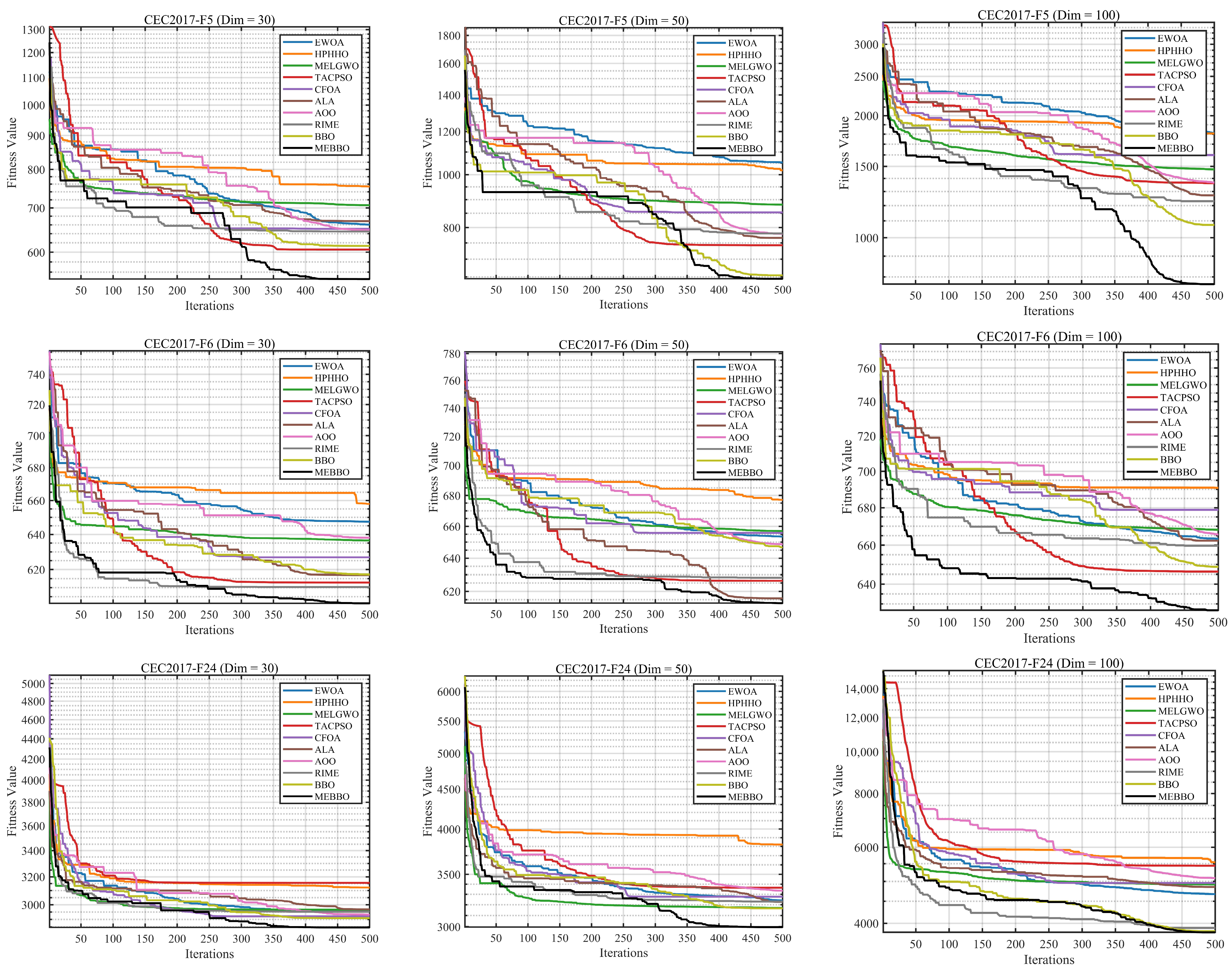
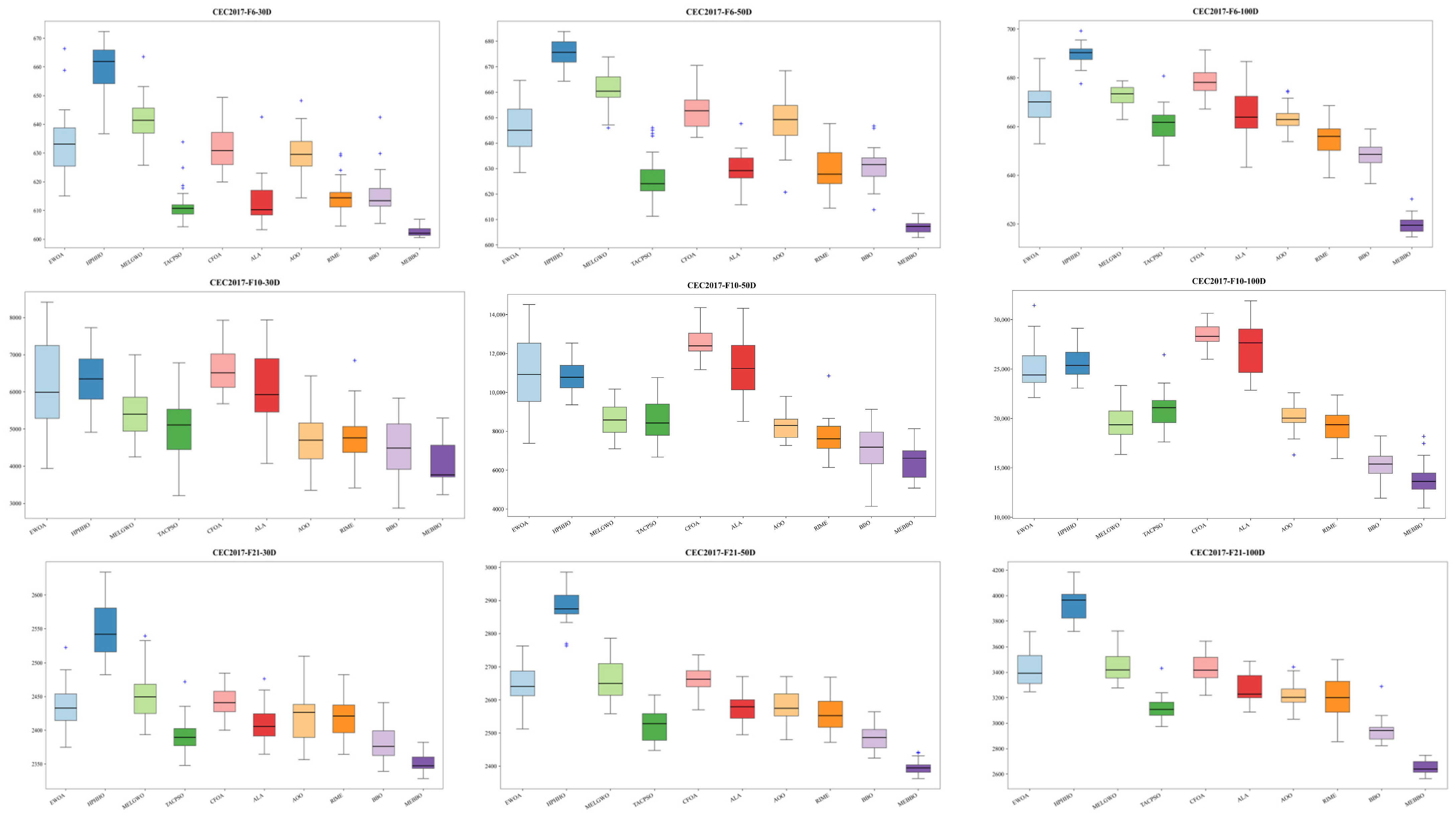
Figure 4 and Figure 5 present the convergence curves and boxplots of MEBBO on selected representative functions. As shown in Figure 4, after an initial rapid decline during the early iterations, MEBBO enters a relatively flat plateau phase before accelerating its convergence again. This indicates the algorithm’s ability to escape local optima during initial exploration and achieve efficient convergence near global optimal regions. Figure 5 shows that under varying dimensional conditions, MEBBO’s boxplots exhibit lower overall positions and narrower distribution ranges than those of the other algorithms, with smaller mean values and standard deviations—a pattern consistent with the numerical results presented in Table 6, Table 7 and Table 8.

Table 9. Wilcoxon Rank-Sum Test results of MEBBO and 9 algorithms on the CEC 2017 (Dim = 30).

Algorithm	EWOA	HPHHO	MELGWO	TACPSO	CFOA	ALA	AOO	RIME	BBO
F1	3.0199 × 10−11	3.0199 × 10−11	3.0199 × 10−11	3.7108 × 10−1	3.0199 × 10−11	4.0772 × 10−11	3.0199 × 10−11	3.0199 × 10−11	2.2360 × 10−2
F2	3.0199 × 10−11	1.2118 × 10−12	3.0199 × 10−11	5.0723 × 10−10	3.0199 × 10−11	3.0199 × 10−11	3.0199 × 10−11	5.4941 × 10−11	7.2208 × 10−6
F3	3.0199 × 10−11	3.6897 × 10−11	3.1589 × 10−10	1.9568 × 10−10	4.5043 × 10−11	1.3594 × 10−7	3.4742 × 10−10	3.1589 × 10−10	1.5798 × 10−1
F4	4.3531 × 10−5	3.0199 × 10−11	3.1967 × 10−9	9.3341 × 10−2	3.0199 × 10−11	3.1573 × 10−5	1.5178 × 10−3	6.0971 × 10−3	5.0114 × 10−1
F5	3.0199 × 10−11	3.0199 × 10−11	3.0199 × 10−11	1.4110 × 10−9	3.0199 × 10−11	1.9568 × 10−10	6.6955 × 10−11	1.0937 × 10−10	1.0105 × 10−8
F6	3.0199 × 10−11	3.0199 × 10−11	3.0199 × 10−11	8.9934 × 10−11	3.0199 × 10−11	1.2057 × 10−10	3.0199 × 10−11	4.0772 × 10−11	3.6897 × 10−11
F7	3.0199 × 10−11	3.0199 × 10−11	3.0199 × 10−11	1.2870 × 10−9	3.0199 × 10−11	7.3891 × 10−11	6.6955 × 10−11	1.4643 × 10−10	6.1210 × 10−10
F8	3.0199 × 10−11	3.0199 × 10−11	3.0199 × 10−11	7.3891 × 10−11	3.0199 × 10−11	3.3384 × 10−11	3.0199 × 10−11	3.3384 × 10−11	6.6955 × 10−11
F9	3.0199 × 10−11	3.0199 × 10−11	3.0199 × 10−11	3.0199 × 10−11	3.0199 × 10−11	3.0199 × 10−11	3.0199 × 10−11	3.0199 × 10−11	3.0199 × 10−11
F10	2.4386 × 10−9	4.9752 × 10−11	1.2023 × 10−8	1.3367 × 10−5	3.0199 × 10−11	2.0338 × 10−9	1.7836 × 10−4	3.7704 × 10−4	2.6077 × 10−2
F11	2.8314 × 10−8	3.0199 × 10−11	7.3891 × 10−11	1.6285 × 10−2	7.3891 × 10−11	1.0315 × 10−2	4.6390 × 10−5	7.7725 × 10−9	9.7052 × 10−1
F12	6.5486 × 10−4	3.0199 × 10−11	4.0772 × 10−11	1.0869 × 10−1	3.0199 × 10−11	9.4683 × 10−3	2.4386 × 10−9	1.4110 × 10−9	9.2113 × 10−5
F13	6.2828 × 10−6	3.0199 × 10−11	2.0283 × 10−7	5.3221 × 10−3	7.2827 × 10−1	9.7052 × 10−1	2.3168 × 10−6	2.8314 × 10−8	2.8129 × 10−2
F14	7.3803 × 10−10	1.9568 × 10−10	1.2541 × 10−7	7.7272 × 10−2	4.4642 × 10−1	1.0937 × 10−10	8.8411 × 10−7	5.8587 × 10−6	5.5699 × 10−3
F15	1.8575 × 10−3	3.9648 × 10−8	5.2978 × 10−1	2.1959 × 10−7	3.2651 × 10−2	3.4029 × 10−1	2.6784 × 10−6	3.7904 × 10−1	9.4696 × 10−1
F16	1.8575 × 10−3	4.1825 × 10−9	1.6062 × 10−6	5.0120 × 10−2	1.4932 × 10−4	9.0307 × 10−4	1.0035 × 10−3	9.0688 × 10−3	5.5546 × 10−2
F17	3.9648 × 10−8	7.1186 × 10−9	6.0459 × 10−7	1.2541 × 10−7	3.8481 × 10−3	1.8682 × 10−5	1.3594 × 10−7	2.4913 × 10−6	3.8307 × 10−5
F18	2.5306 × 10−4	1.1077 × 10−6	6.1452 × 10−2	1.4128 × 10−1	8.1200 × 10−4	2.1947 × 10−8	4.8413 × 10−2	5.9706 × 10−5	5.4933 × 10−1
F19	1.3017 × 10−3	1.2057 × 10−10	2.5188 × 10−1	6.7362 × 10−6	2.6784 × 10−6	5.6922 × 10−1	1.8567 × 10−9	2.9727 × 10−1	2.5188 × 10−1
F20	9.2603 × 10−9	4.1178 × 10−6	1.8731 × 10−7	5.9706 × 10−5	3.0059 × 10−4	8.8411 × 10−7	7.5991 × 10−7	3.3386 × 10−3	2.9205 × 10−2
F21	4.0772 × 10−11	3.0199 × 10−11	3.0199 × 10−11	8.1014 × 10−10	3.0199 × 10−11	6.0658 × 10−11	8.1527 × 10−11	4.9752 × 10−11	7.0430 × 10−7
F22	3.0199 × 10−11	3.0199 × 10−11	3.0199 × 10−11	3.3384 × 10−11	3.0199 × 10−11	3.0199 × 10−11	3.3384 × 10−11	3.0199 × 10−11	6.3560 × 10−5
F23	6.1210 × 10−10	4.9752 × 10−11	4.9752 × 10−11	3.0811 × 10−8	4.5043 × 10−11	2.2273 × 10−9	7.3891 × 10−11	1.1737 × 10−9	1.2477 × 10−4
F24	3.3384 × 10−11	3.0199 × 10−11	3.0199 × 10−11	5.4941 × 10−11	3.0199 × 10−11	6.6955 × 10−11	4.9752 × 10−11	1.6132 × 10−10	4.6856 × 10−8
F25	1.1674 × 10−5	3.0199 × 10−11	1.3289 × 10−10	6.7869 × 10−2	3.0199 × 10−11	4.2175 × 10−4	7.1988 × 10−5	3.8349 × 10−6	6.6273 × 10−1
F26	4.9980 × 10−9	3.8249 × 10−9	3.0199 × 10−11	2.6243 × 10−3	2.5306 × 10−4	2.1544 × 10−10	6.7362 × 10−6	7.3803 × 10−10	2.7726 × 10−5
F27	2.3168 × 10−6	3.0199 × 10−11	2.8314 × 10−8	7.2951 × 10−4	1.0188 × 10−5	4.7335 × 10−1	2.5721 × 10−7	4.2896 × 10−1	2.3985 × 10−1
F28	2.8716 × 10−10	3.0199 × 10−11	3.0199 × 10−11	1.3111 × 10−8	3.0199 × 10−11	4.6159 × 10−10	3.8249 × 10−9	1.6132 × 10−10	2.4994 × 10−3
F29	1.8567 × 10−9	6.0658 × 10−11	1.0937 × 10−10	1.2493 × 10−5	3.1589 × 10−10	4.9980 × 10−9	4.6856 × 10−8	1.3111 × 10−8	5.9706 × 10−5
F30	3.3384 × 10−11	3.0199 × 10−11	1.1737 × 10−9	2.0152 × 10−8	5.0723 × 10−10	2.7726 × 10−5	4.0772 × 10−11	7.0430 × 10−7	8.7663 × 10−1

,

Table 10. Wilcoxon Rank-Sum Test results of MEBBO and 9 algorithms on the CEC 2017 (Dim = 50).

Algorithm	EWOA	HPHHO	MELGWO	TACPSO	CFOA	ALA	AOO	RIME	BBO
F1	3.0199 × 10−11	3.0199 × 10−11	3.0199 × 10−11	3.0199 × 10−11	3.0199 × 10−11	3.0199 × 10−11	3.0199 × 10−11	3.0199 × 10−11	2.9215 × 10−9
F2	3.0199 × 10−11	1.2118 × 10−12	3.0199 × 10−11	3.0199 × 10−11	3.0199 × 10−11	3.0199 × 10−11	3.0199 × 10−11	3.0199 × 10−11	2.4386 × 10−9
F3	3.0199 × 10−11	1.1077 × 10−6	1.3594 × 10−7	1.9568 × 10−10	1.1737 × 10−9	3.3679 × 10−4	7.7725 × 10−9	5.4941 × 10−11	9.7917 × 10−5
F4	3.0199 × 10−11	3.0199 × 10−11	3.0199 × 10−11	3.8349 × 10−6	3.0199 × 10−11	2.6695 × 10−9	6.5183 × 10−9	3.3242 × 10−6	5.7929 × 10−1
F5	3.0199 × 10−11	3.0199 × 10−11	3.0199 × 10−11	8.9934 × 10−11	3.0199 × 10−11	3.0199 × 10−11	3.0199 × 10−11	3.0199 × 10−11	4.1997 × 10−10
F6	3.0199 × 10−11	3.0199 × 10−11	3.0199 × 10−11	3.6897 × 10−11	3.0199 × 10−11	3.0199 × 10−11	3.0199 × 10−11	3.0199 × 10−11	3.0199 × 10−11
F7	3.0199 × 10−11	3.0199 × 10−11	3.0199 × 10−11	3.0199 × 10−11	3.0199 × 10−11	3.0199 × 10−11	3.0199 × 10−11	3.0199 × 10−11	3.0199 × 10−11
F8	3.0199 × 10−11	3.0199 × 10−11	3.0199 × 10−11	3.0199 × 10−11	3.0199 × 10−11	3.0199 × 10−11	3.0199 × 10−11	3.0199 × 10−11	4.5043 × 10−11
F9	3.0199 × 10−11	3.0199 × 10−11	3.0199 × 10−11	3.6897 × 10−11	3.0199 × 10−11	3.0199 × 10−11	3.0199 × 10−11	3.6897 × 10−11	3.0199 × 10−11
F10	5.4941 × 10−11	3.0199 × 10−11	1.2870 × 10−9	1.4110 × 10−9	3.0199 × 10−11	3.0199 × 10−11	6.7220 × 10−10	9.5139 × 10−6	1.5638 × 10−2
F11	3.0199 × 10−11	3.0199 × 10−11	3.0199 × 10−11	2.6099 × 10−10	3.0199 × 10−11	4.5043 × 10−11	3.0199 × 10−11	4.0772 × 10−11	2.4157 × 10−2
F12	3.8053 × 10−7	3.0199 × 10−11	3.0199 × 10−11	9.4696 × 10−1	3.0199 × 10−11	2.7726 × 10−5	3.0199 × 10−11	3.0199 × 10−11	4.2039 × 10−1
F13	3.0103 × 10−7	3.0199 × 10−11	3.6897 × 10−11	3.3681 × 10−5	1.0937 × 10−10	1.1199 × 10−1	3.9881 × 10−4	4.0772 × 10−11	2.8378 × 10−1
F14	1.5465 × 10−9	3.3384 × 10−11	1.3594 × 10−7	5.8282 × 10−3	2.7719 × 10−1	4.6390 × 10−5	1.1567 × 10−7	3.8202 × 10−10	3.7704 × 10−4
F15	1.7290 × 10−6	3.0199 × 10−11	2.5721 × 10−7	7.2208 × 10−6	2.1702 × 10−1	5.2978 × 10−1	1.0188 × 10−5	5.4941 × 10−11	3.2553 × 10−1
F16	1.2870 × 10−9	3.3384 × 10−11	2.9215 × 10−9	1.4932 × 10−4	2.6695 × 10−9	1.8500 × 10−8	1.1077 × 10−6	1.8567 × 10−9	1.5178 × 10−3
F17	3.5201 × 10−7	3.8249 × 10−9	1.7294 × 10−7	1.2212 × 10−2	6.6689 × 10−3	2.3897 × 10−8	3.9167 × 10−2	2.4327 × 10−5	1.3732 × 10−1
F18	1.3832 × 10−2	6.5261 × 10−7	3.1573 × 10−5	1.3832 × 10−2	4.9178 × 10−1	8.8829 × 10−6	1.7836 × 10−4	5.2650 × 10−5	7.8446 × 10−1
F19	8.9934 × 10−11	4.0772 × 10−11	5.5611 × 10−4	1.9568 × 10−10	1.6062 × 10−6	1.3289 × 10−10	7.1186 × 10−9	5.4620 × 10−6	7.2884 × 10−3
F20	2.1947 × 10−8	4.8011 × 10−7	2.0023 × 10−6	2.7829 × 10−7	4.4205 × 10−6	2.2273 × 10−9	2.0023 × 10−6	8.8411 × 10−7	4.7138 × 10−4
F21	3.0199 × 10−11	3.0199 × 10−11	3.0199 × 10−11	3.0199 × 10−11	3.0199 × 10−11	3.0199 × 10−11	3.0199 × 10−11	3.0199 × 10−11	8.9934 × 10−11
F22	3.6897 × 10−11	3.3384 × 10−11	9.9186 × 10−11	5.0723 × 10−10	3.3520 × 10−8	3.0199 × 10−11	1.8731 × 10−7	3.1967 × 10−9	1.8575 × 10−3
F23	3.0199 × 10−11	3.0199 × 10−11	3.0199 × 10−11	4.0772 × 10−11	3.0199 × 10−11	3.3384 × 10−11	3.0199 × 10−11	4.0772 × 10−11	8.1014 × 10−10
F24	3.0199 × 10−11	3.0199 × 10−11	3.0199 × 10−11	3.0199 × 10−11	3.0199 × 10−11	3.3384 × 10−11	3.0199 × 10−11	3.0199 × 10−11	3.4971 × 10−9
F25	3.1589 × 10−10	3.0199 × 10−11	3.0199 × 10−11	1.3853 × 10−6	3.0199 × 10−11	5.4941 × 10−11	3.8202 × 10−10	9.5332 × 10−7	5.0114 × 10−1
F26	8.1014 × 10−10	3.3384 × 10−11	4.9752 × 10−11	5.5611 × 10−4	5.4941 × 10−11	3.4971 × 10−9	1.4733 × 10−7	2.0338 × 10−9	4.4205 × 10−6
F27	1.5465 × 10−9	3.0199 × 10−11	3.6897 × 10−11	2.0023 × 10−6	3.3384 × 10−11	2.9590 × 10−5	3.0199 × 10−11	3.6459 × 10−8	9.2344 × 10−1
F28	3.3384 × 10−11	3.0199 × 10−11	3.0199 × 10−11	1.0937 × 10−10	3.0199 × 10−11	3.3384 × 10−11	3.0199 × 10−11	3.4742 × 10−10	3.3874 × 10−2
F29	3.0939 × 10−6	3.0199 × 10−11	3.3384 × 10−11	2.4913 × 10−6	7.3891 × 10−11	3.6459 × 10−8	1.1737 × 10−9	3.8202 × 10−10	4.9426 × 10−5
F30	3.0199 × 10−11	3.0199 × 10−11	1.3289 × 10−10	3.0199 × 10−11	3.0199 × 10−11	3.0199 × 10−11	3.0199 × 10−11	5.4941 × 10−11	2.6433 × 10−1

and

Table 11. Wilcoxon Rank-Sum Test results of MEBBO and 9 algorithms on the CEC 2017 (Dim = 100).

Algorithm	EWOA	HPHHO	MELGWO	TACPSO	CFOA	ALA	AOO	RIME	BBO
F1	3.0199 × 10−11	3.0199 × 10−11	3.0199 × 10−11	3.0199 × 10−11	3.0199 × 10−11	3.0199 × 10−11	3.0199 × 10−11	3.0199 × 10−11	4.5043 × 10−11
F2	3.0199 × 10−11	1.2118 × 10−12	3.0199 × 10−11	3.0199 × 10−11	3.0199 × 10−11	3.0199 × 10−11	3.0199 × 10−11	3.0199 × 10−11	3.6897 × 10−11
F3	3.6897 × 10−11	1.5465 × 10−9	4.7445 × 10−6	2.3768 × 10−7	2.0621 × 10−1	3.0811 × 10−8	5.0723 × 10−10	7.3891 × 10−11	1.6285 × 10−2
F4	3.0199 × 10−11	3.0199 × 10−11	3.0199 × 10−11	3.0199 × 10−11	3.0199 × 10−11	3.0199 × 10−11	3.0199 × 10−11	3.0199 × 10−11	7.0881 × 10−8
F5	3.0199 × 10−11	3.0199 × 10−11	3.0199 × 10−11	3.0199 × 10−11	3.0199 × 10−11	3.0199 × 10−11	3.0199 × 10−11	3.0199 × 10−11	3.0199 × 10−11
F6	3.0199 × 10−11	3.0199 × 10−11	3.0199 × 10−11	3.0199 × 10−11	3.0199 × 10−11	3.0199 × 10−11	3.0199 × 10−11	3.0199 × 10−11	3.0199 × 10−11
F7	3.0199 × 10−11	3.0199 × 10−11	3.0199 × 10−11	3.0199 × 10−11	3.0199 × 10−11	3.0199 × 10−11	3.0199 × 10−11	3.0199 × 10−11	3.0199 × 10−11
F8	3.0199 × 10−11	3.0199 × 10−11	3.0199 × 10−11	3.0199 × 10−11	3.0199 × 10−11	3.0199 × 10−11	3.0199 × 10−11	3.0199 × 10−11	3.0199 × 10−11
F9	3.0199 × 10−11	3.0199 × 10−11	3.0199 × 10−11	3.0199 × 10−11	3.0199 × 10−11	3.0199 × 10−11	3.0199 × 10−11	3.0199 × 10−11	3.0199 × 10−11
F10	3.0199 × 10−11	3.0199 × 10−11	6.6955 × 10−11	4.5043 × 10−11	3.0199 × 10−11	3.0199 × 10−11	4.5043 × 10−11	1.4643 × 10−10	2.3885 × 10−4
F11	3.0199 × 10−11	3.0199 × 10−11	3.0199 × 10−11	3.0199 × 10−11	3.0199 × 10−11	3.0199 × 10−11	3.0199 × 10−11	3.0199 × 10−11	3.1466 × 10−2
F12	3.0199 × 10−11	3.0199 × 10−11	3.0199 × 10−11	3.6897 × 10−11	3.0199 × 10−11	3.0199 × 10−11	3.0199 × 10−11	3.0199 × 10−11	7.2884 × 10−3
F13	3.0199 × 10−11	3.0199 × 10−11	3.0199 × 10−11	8.6634 × 10−5	3.0199 × 10−11	3.0199 × 10−11	3.3384 × 10−11	3.0199 × 10−11	8.1975 × 10−7
F14	1.2023 × 10−8	3.3384 × 10−11	5.5999 × 10−7	2.0681 × 10−2	1.2493 × 10−5	2.5188 × 10−1	2.1540 × 10−6	1.8731 × 10−7	8.7710 × 10−2
F15	2.4913 × 10−6	3.0199 × 10−11	3.0199 × 10−11	4.4205 × 10−6	3.0199 × 10−11	3.0811 × 10−8	5.0922 × 10−8	3.0199 × 10−11	6.9125 × 10−4
F16	4.1997 × 10−10	3.0199 × 10−11	3.0199 × 10−11	4.1825 × 10−9	3.0199 × 10−11	3.0199 × 10−11	9.9186 × 10−11	4.0772 × 10−11	1.1738 × 10−3
F17	1.9568 × 10−10	3.0199 × 10−11	3.3384 × 10−11	6.5183 × 10−9	1.7769 × 10−10	1.3289 × 10−10	3.5708 × 10−6	1.6947 × 10−9	1.1199 × 10−1
F18	6.6955 × 10−11	1.0937 × 10−10	4.0840 × 10−5	6.4142 × 10−1	3.0418 × 10−1	1.7145 × 10−1	5.0922 × 10−8	8.1527 × 10−11	3.0339 × 10−3
F19	2.8790 × 10−6	3.0199 × 10−11	3.3384 × 10−11	2.0283 × 10−7	1.9568 × 10−10	1.8500 × 10−8	9.2603 × 10−9	3.0199 × 10−11	9.6263 × 10−2
F20	6.1210 × 10−10	3.2555 × 10−7	2.6806 × 10−4	4.9980 × 10−9	9.9186 × 10−11	3.0199 × 10−11	1.3853 × 10−6	1.4294 × 10−8	8.6844 × 10−3
F21	3.0199 × 10−11	3.0199 × 10−11	3.0199 × 10−11	3.0199 × 10−11	3.0199 × 10−11	3.0199 × 10−11	3.0199 × 10−11	3.0199 × 10−11	3.0199 × 10−11
F22	3.0199 × 10−11	3.0199 × 10−11	9.9186 × 10−11	8.9934 × 10−11	3.0199 × 10−11	3.0199 × 10−11	3.0199 × 10−11	5.4941 × 10−11	2.9590 × 10−5
F23	3.0199 × 10−11	3.0199 × 10−11	3.0199 × 10−11	3.0199 × 10−11	3.0199 × 10−11	3.0199 × 10−11	3.0199 × 10−11	3.0199 × 10−11	3.4742 × 10−10
F24	3.0199 × 10−11	3.0199 × 10−11	3.0199 × 10−11	3.0199 × 10−11	3.0199 × 10−11	3.0199 × 10−11	3.0199 × 10−11	4.9752 × 10−11	7.1186 × 10−9
F25	3.0199 × 10−11	3.0199 × 10−11	3.0199 × 10−11	3.0199 × 10−11	3.0199 × 10−11	3.0199 × 10−11	3.0199 × 10−11	1.6132 × 10−10	8.5000 × 10−2
F26	3.0199 × 10−11	3.0199 × 10−11	3.0199 × 10−11	2.3897 × 10−8	3.0199 × 10−11	3.0199 × 10−11	3.0199 × 10−11	3.0199 × 10−11	8.8910 × 10−10
F27	1.2057 × 10−10	3.0199 × 10−11	3.0199 × 10−11	3.9648 × 10−8	3.0199 × 10−11	1.1077 × 10−6	3.3384 × 10−11	6.0658 × 10−11	1.1747 × 10−4
F28	3.0199 × 10−11	3.0199 × 10−11	3.0199 × 10−11	3.0199 × 10−11	3.0199 × 10−11	3.0199 × 10−11	3.0199 × 10−11	3.0199 × 10−11	1.1738 × 10−3
F29	2.3768 × 10−7	3.0199 × 10−11	3.0199 × 10−11	6.7362 × 10−6	3.0199 × 10−11	4.6856 × 10−8	1.3289 × 10−10	9.9186 × 10−11	7.1988 × 10−5
F30	6.5671 × 10−2	3.0199 × 10−11	3.0199 × 10−11	1.4412 × 10−2	3.0199 × 10−11	3.4971 × 10−9	3.0199 × 10−11	3.0199 × 10−11	1.3272 × 10−2

present the Wilcoxon rank-sum test results comparing MEBBO with nine benchmark algorithms across various dimensions of the CEC 2017 test set. Overall, the majority of comparisons yielded p-values below 0.05, indicating statistically significant differences between MEBBO and most competing algorithms. This demonstrates that its performance improvements are not attributable to random fluctuations but instead possess strong statistical significance. Notably, when compared with algorithms such as EWOA, MELGWO, CFOA, AOO, and RIME, MEBBO exhibited significant performance differences across most test functions in 30-dimensional, 50-dimensional, and 100-dimensional datasets, further validating its advantages in solution accuracy and stability.

The test results across multiple dimensions demonstrate that MEBBO maintains more stable and more pronounced statistical superiority over the other algorithms as the problem dimensionality increases. Under the 30-dimensional condition, MEBBO shows no significant differences from TACPSO, ALA, and the original BBO on a limited number of functions. However, at the 50-dimensional and 100-dimensional levels, such “insignificant differences” become markedly reduced, indicating MEBBO’s enhanced performance in medium-to-high-dimensional complex optimization problems. Notably, compared with the original BBO, MEBBO achieves statistically significant differences on most functions at 50 and 100 dimensions, demonstrating that the proposed multi-strategy enhancement mechanism effectively improves the algorithm’s optimization capabilities in complex search environments. Overall, the Wilcoxon rank-sum test results provide further statistical support for MEBBO’s superiority and robustness relative to all benchmark algorithms.

Table 12. Results of the Friedman average rank test on CEC2017.

Suites	CEC2017
Dimensions	30		50		100
Algorithm	Avg Rank	Overall Rank	Avg Rank	Overall Rank	Avg Rank	Overall Rank
EWOA	6.40	7	6.53	7	6.83	7
HPHHO	9.57	10	9.13	10	8.87	10
MELGWO	8.23	9	7.63	9	7.43	8
TACPSO	4.10	3	4.33	3	4.77	4
CFOA	6.53	8	7.40	8	7.83	9
ALA	4.47	4	5.13	5	5.53	6
AOO	6.07	6	5.67	6	5.17	5
RIME	5.03	5	4.97	4	4.70	3
BBO	2.90	2	2.60	2	2.53	2
MEBBO	1.70	1	1.60	1	1.33	1

presents the results of the Friedman test. MEBBO consistently ranked first overall across all dimensional conditions, with Friedman rank values of 1.70, 1.60, and 1.33 for the 30-dimensional, 50-dimensional, and 100-dimensional datasets, respectively. BBO maintained a stable second-place ranking across all dimensions, while TACPSO and RIME demonstrated strong performance, securing positions from third to fifth in various dimensions. In contrast, AOO, EWOA, and ALA exhibited moderate rankings, whereas HPHHO, MELGWO, and CFOA ranked relatively lower overall. 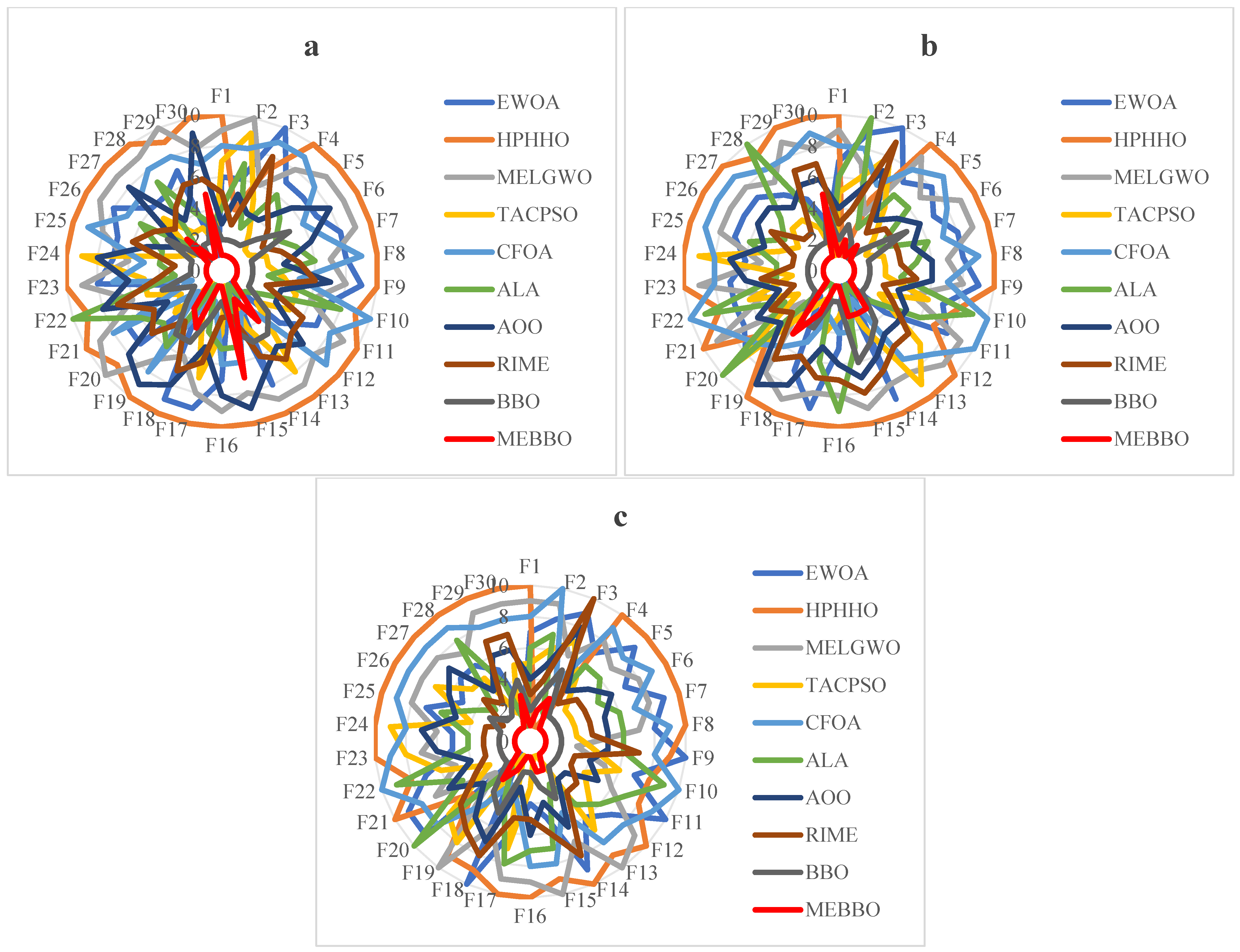Figure 6a–c display radar charts of the Friedman test results for the 30-dimensional, 50-dimensional, and 100-dimensional conditions, respectively. Consistent with the findings in Table 12, these visualizations clearly demonstrate MEBBO’s consistent position at the innermost location, further validating its highest comprehensive ranking.

4.5. Sensitivity Analysis

To examine the influence of the elite proportion $N_e$ in the elite pool-enhanced exploration strategy, a sensitivity analysis was conducted by setting $N_{\mathrm{e}}$ to 0.1, 0.2, 0.3, 0.4, and 0.5, respectively. As shown in

Table 13. Results of sensitivity analysis.

Function	Metric	MEBBO1	MEBBO2	MEBBO3	MEBBO4	MEBBO5
F1	Mean	4.3224 × 104	5.1424 × 104	5.3480 × 104	6.1398 × 104	6.5137 × 104
	Std	4.2655 × 104	3.2037 × 104	4.2402 × 104	3.9314 × 104	6.3668 × 104
F2	Mean	3.2744 × 1012	1.0731 × 1013	1.4232 × 1013	3.5671 × 1012	5.0277 × 1012
	Std	4.5181 × 1012	2.1728 × 1013	5.7313 × 1013	5.9549 × 1012	1.2629 × 1013
F3	Mean	1.8614 × 104	1.5770 × 104	1.3657 × 104	1.5766 × 104	1.5280 × 104
	Std	6.2512 × 103	6.2104 × 103	7.2159 × 103	5.5837 × 103	7.6894 × 103
F4	Mean	5.0480 × 102	4.9528 × 102	5.0466 × 102	5.0651 × 102	5.0069 × 102
	Std	2.0654 × 101	2.2891 × 101	2.6739 × 101	1.8066 × 101	2.0868 × 101
F5	Mean	5.4903 × 102	5.4617 × 102	5.4933 × 102	5.5024 × 102	5.4843 × 102
	Std	1.3184 × 101	1.0843 × 101	1.5387 × 101	1.4599 × 101	1.0445 × 101
F6	Mean	6.0266 × 102	6.0253 × 102	6.0214 × 102	6.0196 × 102	6.0300 × 102
	Std	1.4606 × 100	1.6055 × 100	1.1809 × 100	1.1840 × 100	2.8921 × 100
F7	Mean	7.9602 × 102	7.8940 × 102	7.9003 × 102	8.0158 × 102	8.0295 × 102
	Std	2.0909 × 101	1.6559 × 101	1.3390 × 101	2.5024 × 101	1.9332 × 101
F8	Mean	8.4116 × 102	8.4338 × 102	8.4548 × 102	8.4659 × 102	8.4362 × 102
	Std	1.4325 × 101	1.1246 × 101	1.1868 × 101	9.9830 × 100	1.2751 × 101
F9	Mean	9.4450 × 102	9.3288 × 102	9.3021 × 102	9.2962 × 102	9.4666 × 102
	Std	6.6622 × 101	3.5228 × 101	3.8625 × 101	2.2405 × 101	3.6210 × 101
F10	Mean	4.1615 × 103	3.9571 × 103	4.0050 × 103	3.7387 × 103	3.9854 × 103
	Std	6.1905 × 102	7.9771 × 102	7.5427 × 102	6.2422 × 102	5.6680 × 102
F11	Mean	1.2318 × 103	1.2428 × 103	1.2531 × 103	1.2454 × 103	1.2566 × 103
	Std	4.6263 × 101	3.4416 × 101	4.6918 × 101	4.5713 × 101	5.8867 × 101
F12	Mean	1.8244 × 106	1.9464 × 106	1.9514 × 106	1.9654 × 106	1.4379 × 106
	Std	8.6389 × 105	1.5192 × 106	9.1584 × 105	1.5725 × 106	7.8473 × 105
F13	Mean	4.3699 × 104	4.2570 × 104	5.1359 × 104	4.7185 × 104	4.4071 × 104
	Std	2.1523 × 104	1.9958 × 104	2.6329 × 104	2.8649 × 104	2.1452 × 104
F14	Mean	1.3754 × 104	1.9070 × 104	1.4429 × 104	1.2940 × 104	2.0713 × 104
	Std	8.1773 × 103	1.1456 × 104	1.0275 × 104	9.8571 × 103	2.1034 × 104
F15	Mean	2.9649 × 104	2.0102 × 104	1.7720 × 104	2.7117 × 104	2.2396 × 104
	Std	1.5803 × 104	1.0758 × 104	9.5264 × 103	1.9285 × 104	1.4387 × 104
F16	Mean	2.4931 × 103	2.4793 × 103	2.3988 × 103	2.4299 × 103	2.4720 × 103
	Std	2.7296 × 102	3.0508 × 102	2.6206 × 102	2.7068 × 102	2.2693 × 102
F17	Mean	2.0075 × 103	1.9469 × 103	1.9715 × 103	1.9974 × 103	1.9647 × 103
	Std	1.8530 × 102	1.7488 × 102	1.4761 × 102	2.0276 × 102	1.5786 × 102
F18	Mean	5.4087 × 105	5.3919 × 105	3.6863 × 105	4.0212 × 105	5.6003 × 105
	Std	5.6064 × 105	5.4468 × 105	4.4603 × 105	2.8680 × 105	3.6737 × 105
F19	Mean	1.6403 × 104	2.1884 × 104	1.9253 × 104	2.1582 × 104	1.5373 × 104
	Std	1.4422 × 104	2.1534 × 104	1.8404 × 104	1.7982 × 104	8.6541 × 103
F20	Mean	2.2975 × 103	2.3158 × 103	2.3040 × 103	2.3116 × 103	2.2912 × 103
	Std	8.6857 × 101	1.0996 × 102	8.3861 × 101	9.4442 × 101	9.2825 × 101
F21	Mean	2.3498 × 103	2.3475 × 103	2.3518 × 103	2.3559 × 103	2.3472 × 103
	Std	1.1673 × 101	1.2426 × 101	1.1733 × 101	1.3546 × 101	1.0864 × 101
F22	Mean	2.4004 × 103	2.3022 × 103	2.3026 × 103	2.3020 × 103	2.3023 × 103
	Std	5.3532 × 102	1.3683 × 100	1.3046 × 100	1.3276 × 100	1.0670 × 100
F23	Mean	2.7145 × 103	2.7058 × 103	2.7089 × 103	2.7088 × 103	2.7131 × 103
	Std	2.5153 × 101	2.3826 × 101	2.4597 × 101	2.0398 × 101	2.4972 × 101
F24	Mean	2.8620 × 103	2.8587 × 103	2.8623 × 103	2.8666 × 103	2.8662 × 103
	Std	1.5648 × 101	1.5683 × 101	1.7918 × 101	1.5699 × 101	2.6805 × 101
F25	Mean	2.9008 × 103	2.8925 × 103	2.8980 × 103	2.8911 × 103	2.8969 × 103
	Std	1.6390 × 101	9.3132 × 100	1.4296 × 101	4.9865 × 100	1.2221 × 101
F26	Mean	3.8713 × 103	4.0926 × 103	3.6197 × 103	3.6700 × 103	3.7051 × 103
	Std	8.2990 × 102	5.6979 × 102	8.0200 × 102	7.8098 × 102	6.8419 × 102
F27	Mean	3.2460 × 103	3.2448 × 103	3.2410 × 103	3.2435 × 103	3.2471 × 103
	Std	1.4319 × 101	1.5981 × 101	1.2628 × 101	1.7514 × 101	1.2256 × 101
F28	Mean	3.2153 × 103	3.2165 × 103	3.2204 × 103	3.2154 × 103	3.2236 × 103
	Std	2.1229 × 101	1.5876 × 101	1.7039 × 101	1.6248 × 101	1.8691 × 101
F29	Mean	3.6493 × 103	3.6267 × 103	3.6601 × 103	3.5842 × 103	3.6739 × 103
	Std	1.5598 × 102	1.4225 × 102	1.5695 × 102	1.2653 × 102	1.4202 × 102
F30	Mean	2.0632 × 105	2.1596 × 105	2.7587 × 105	2.5608 × 105	2.8104 × 105
	Std	1.6151 × 105	1.4911 × 105	2.0387 × 105	1.3726 × 105	2.5178 × 105
Avg Rank		3.13	2.53	3.00	2.93	3.40
Overall Rank		4	1	3	2	5

, different values of $N_e$ lead to noticeable variations in the optimization performance of MEBBO. Among the five parameter settings, MEBBO2, corresponding to $N_e=0.2$, achieves the best overall performance, with the lowest average rank of 2.53. MEBBO4, corresponding to $N_e=0.4$, ranks second with an average rank of 2.93, while MEBBO3 and MEBBO1 obtain average ranks of 3.00 and 3.13, respectively. In contrast, MEBBO5, corresponding to $N_e=0.$5, shows the weakest overall performance, with an average rank of 3.40. These results indicate that the elite proportion has a non-negligible effect on the balance between exploration and exploitation.

Specifically, when $N_e$ is relatively small, such as 0.1, the elite pool contains only a limited number of high-quality individuals. Although this setting can preserve strong selection pressure and avoid excessive population homogenization, it may not provide sufficient guidance information for global exploration, resulting in unstable performance on some complex functions. When $N_e$ increases to 0.2, the algorithm achieves the best overall balance. This setting allows the elite pool to retain enough high-quality individuals to guide the population while maintaining adequate diversity among candidate solutions. As a result, MEBBO with $N_e=0.2$ performs competitively across different types of benchmark functions and obtains the best overall ranking. However, further increasing $N_e$ does not continuously improve the algorithm. When $N_e$ is set to 0.4 or 0.5, more individuals are included in the elite pool, but the quality difference among elite individuals may become less distinct. In particular, an overly large elite proportion may weaken selection pressure and introduce relatively inferior individuals into the guidance mechanism, thereby reducing the effectiveness of elite-based exploration. This phenomenon is reflected in the inferior average rank of MEBBO5.

4.6. Ablation Experiment

To further verify the individual contribution and synergistic effect of the three proposed strategies, an extended ablation experiment was conducted by considering not only the single-strategy variants but also the pairwise strategy combinations. As shown in

Table 14. Results of ablation experiments.

Function	Metric	BBO	MEBBO1	MEBBO2	MEBBO3	MEBBO12	MEBBO13	MEBBO23	MEBBO
F1	Mean	1.3195 × 105	9.7164 × 104	4.4076 × 104	1.0941 × 105	4.4755 × 104	1.3033 × 105	5.6823 × 104	4.8656 × 104
	Std	8.9890 × 104	6.8191 × 104	2.7560 × 104	7.4573 × 104	3.4205 × 104	1.9270 × 105	4.5280 × 104	5.8677 × 104
F2	Mean	6.2313 × 1015	5.9666 × 1014	1.8724 × 1013	1.9747 × 1014	8.9657 × 1012	9.6675 × 1013	4.9560 × 1012	1.0496 × 1013
	Std	3.3270 × 1016	2.7187 × 1015	3.1660 × 1013	6.4543 × 1014	1.2186 × 1013	2.3551 × 1014	8.9468 × 1012	1.5738 × 1013
F3	Mean	2.1908 × 104	2.0690 × 104	1.7646 × 104	1.4870 × 104	2.1004 × 104	2.0116 × 104	1.2778 × 104	1.5618 × 104
	Std	9.5881 × 103	8.6254 × 103	8.0478 × 103	5.2620 × 103	1.0024 × 104	9.6314 × 103	4.8894 × 103	6.9929 × 103
F4	Mean	4.9825 × 102	5.0339 × 102	5.0456 × 102	5.1397 × 102	5.0256 × 102	4.9919 × 102	4.9864 × 102	4.9155 × 102
	Std	2.0972 × 101	1.9977 × 101	1.4190 × 101	2.8486 × 101	1.4881 × 101	2.3049 × 101	2.5476 × 101	2.7091 × 101
F5	Mean	6.0582 × 102	5.9449 × 102	5.3864 × 102	5.9882 × 102	5.4116 × 102	5.9896 × 102	5.4951 × 102	5.4763 × 102
	Std	2.1255 × 101	2.0302 × 101	1.1703 × 101	2.6803 × 101	8.8529 × 100	2.7499 × 101	1.1256 × 101	1.3180 × 101
F6	Mean	6.1754 × 102	6.1628 × 102	6.0195 × 102	6.1755 × 102	6.0192 × 102	6.1329 × 102	6.0230 × 102	6.0234 × 102
	Std	7.2237 × 100	7.9008 × 100	1.1418 × 100	7.3549 × 100	1.0353 × 100	8.0742 × 100	1.5619 × 100	1.4050 × 100
F7	Mean	8.6897 × 102	8.6870 × 102	7.8400 × 102	8.6958 × 102	7.9173 × 102	8.6696 × 102	7.9512 × 102	7.9031 × 102
	Std	4.2749 × 101	4.5820 × 101	1.4136 × 101	3.4854 × 101	1.7577 × 101	3.5563 × 101	2.0409 × 101	1.4579 × 101
F8	Mean	8.8170 × 102	8.8141 × 102	8.3499 × 102	8.8525 × 102	8.3924 × 102	8.8358 × 102	8.4709 × 102	8.4566 × 102
	Std	2.1563 × 101	1.7561 × 101	9.4735 × 100	1.9215 × 101	1.4241 × 101	2.2333 × 101	1.7816 × 101	1.0597 × 101
F9	Mean	2.1396 × 103	2.1606 × 103	9.2807 × 102	2.1285 × 103	9.3382 × 102	1.9757 × 103	9.4028 × 102	9.4038 × 102
	Std	5.2942 × 102	5.4946 × 102	3.0529 × 101	6.5087 × 102	2.8875 × 101	5.9546 × 102	3.3375 × 101	5.6399 × 101
F10	Mean	4.2859 × 103	4.3744 × 103	3.8594 × 103	4.6089 × 103	3.7811 × 103	4.3855 × 103	3.9970 × 103	4.1048 × 103
	Std	4.6937 × 102	7.0137 × 102	5.9283 × 102	6.1157 × 102	6.5402 × 102	6.7287 × 102	6.7199 × 102	7.0140 × 102
F11	Mean	1.2807 × 103	1.2658 × 103	1.2803 × 103	1.2419 × 103	1.2775 × 103	1.2632 × 103	1.2409 × 103	1.2471 × 103
	Std	5.2724 × 101	4.5043 × 101	5.6133 × 101	5.6773 × 101	4.4117 × 101	5.5631 × 101	4.6293 × 101	4.5041 × 101
F12	Mean	3.0069 × 106	3.7761 × 106	2.5192 × 106	3.4572 × 106	2.0370 × 106	3.5071 × 106	1.7002 × 106	1.7990 × 106
	Std	2.5745 × 106	3.2742 × 106	1.8143 × 106	2.0859 × 106	1.2556 × 106	2.5712 × 106	1.1027 × 106	1.4060 × 106
F13	Mean	5.0121 × 104	5.3334 × 104	5.9482 × 104	3.9231 × 104	6.0149 × 104	5.1306 × 104	4.4537 × 104	4.1490 × 104
	Std	2.1690 × 104	3.1039 × 104	2.3405 × 104	2.1749 × 104	2.7930 × 104	2.3817 × 104	2.5094 × 104	1.9001 × 104
F14	Mean	5.0549 × 104	3.4523 × 104	2.6653 × 104	2.7297 × 104	2.7447 × 104	3.7975 × 104	1.4570 × 104	1.9637 × 104
	Std	4.6645 × 104	2.4728 × 104	2.3705 × 104	1.7661 × 104	2.4806 × 104	4.0630 × 104	1.3608 × 104	1.6608 × 104
F15	Mean	2.0627 × 104	2.4009 × 104	3.0290 × 104	1.5167 × 104	2.4420 × 104	2.4299 × 104	2.1808 × 104	2.1263 × 104
	Std	1.1767 × 104	1.9980 × 104	1.9763 × 104	9.2653 × 103	1.5358 × 104	1.5676 × 104	9.6280 × 103	1.7513 × 104
F16	Mean	2.6146 × 103	2.5278 × 103	2.3165 × 103	2.6836 × 103	2.4355 × 103	2.5395 × 103	2.4605 × 103	2.5501 × 103
	Std	3.3780 × 102	2.4395 × 102	3.4260 × 102	2.8717 × 102	3.0886 × 102	3.0515 × 102	3.2295 × 102	3.2241 × 102
F17	Mean	2.0938 × 103	2.0767 × 103	1.9447 × 103	2.0515 × 103	1.9476 × 103	2.0202 × 103	1.9633 × 103	2.0006 × 103
	Std	1.6516 × 102	1.7476 × 102	1.2257 × 102	1.8042 × 102	1.4215 × 102	1.9884 × 102	1.5063 × 102	1.7808 × 102
F18	Mean	5.9091 × 105	6.8685 × 105	5.2193 × 105	5.6230 × 105	7.1821 × 105	8.6586 × 105	5.0427 × 105	3.4891 × 105
	Std	6.5424 × 105	6.4615 × 105	4.7998 × 105	6.4451 × 105	6.4281 × 105	8.4222 × 105	7.9128 × 105	2.7319 × 105
F19	Mean	1.7567 × 104	2.4516 × 104	1.8721 × 104	1.4899 × 104	2.2501 × 104	1.8421 × 104	1.5964 × 104	1.9730 × 104
	Std	1.9724 × 104	2.2862 × 104	1.1717 × 104	1.4799 × 104	2.7284 × 104	2.0538 × 104	9.2645 × 103	1.3655 × 104
F20	Mean	2.4880 × 103	2.4689 × 103	2.3157 × 103	2.4907 × 103	2.2839 × 103	2.4830 × 103	2.3510 × 103	2.3244 × 103
	Std	2.0286 × 102	1.5388 × 102	1.3227 × 102	1.7232 × 102	1.1899 × 102	1.6040 × 102	1.0985 × 102	1.0838 × 102
F21	Mean	2.3865 × 103	2.3881 × 103	2.3411 × 103	2.3878 × 103	2.3451 × 103	2.3973 × 103	2.3551 × 103	2.3487 × 103
	Std	2.1857 × 101	2.3447 × 101	1.1986 × 101	2.0939 × 101	1.3506 × 101	2.1062 × 101	1.6108 × 101	1.5386 × 101
F22	Mean	3.3791 × 103	3.2922 × 103	2.7397 × 103	2.9266 × 103	2.7441 × 103	3.1094 × 103	2.4342 × 103	2.3990 × 103
	Std	1.6884 × 103	1.6940 × 103	1.1468 × 103	1.4311 × 103	1.1532 × 103	1.5234 × 103	7.2167 × 102	5.2969 × 102
F23	Mean	2.7543 × 103	2.7527 × 103	2.6921 × 103	2.7778 × 103	2.6965 × 103	2.7450 × 103	2.7207 × 103	2.7121 × 103
	Std	2.8096 × 101	3.6927 × 101	1.2598 × 101	3.5538 × 101	1.2152 × 101	3.1479 × 101	2.7419 × 101	1.9072 × 101
F24	Mean	2.9052 × 103	2.9046 × 103	2.8572 × 103	2.9237 × 103	2.8598 × 103	2.9105 × 103	2.8663 × 103	2.8675 × 103
	Std	2.7378 × 101	2.7312 × 101	1.5772 × 101	3.5570 × 101	1.4709 × 101	2.7361 × 101	2.0827 × 101	2.2687 × 101
F25	Mean	2.9032 × 103	2.9017 × 103	2.8917 × 103	2.9078 × 103	2.8905 × 103	2.9074 × 103	2.8960 × 103	2.8949 × 103
	Std	2.1063 × 101	1.8658 × 101	1.1015 × 101	1.7418 × 101	1.0040 × 101	2.1540 × 101	1.1945 × 101	1.2196 × 101
F26	Mean	4.3134 × 103	4.4262 × 103	3.8887 × 103	3.9871 × 103	3.9661 × 103	4.1400 × 103	3.6565 × 103	3.5081 × 103
	Std	1.3015 × 103	1.1300 × 103	4.3971 × 102	1.3974 × 103	3.6294 × 102	1.2136 × 103	7.6342 × 102	7.2356 × 102
F27	Mean	3.2360 × 103	3.2374 × 103	3.2222 × 103	3.2832 × 103	3.2250 × 103	3.2412 × 103	3.2460 × 103	3.2408 × 103
	Std	1.7051 × 101	1.5440 × 101	1.1046 × 101	2.4119 × 101	1.1183 × 101	1.3240 × 101	1.7612 × 101	1.3750 × 101
F28	Mean	3.2357 × 103	3.2447 × 103	3.2262 × 103	3.2352 × 103	3.2278 × 103	3.2366 × 103	3.2230 × 103	3.2161 × 103
	Std	2.5216 × 101	2.2028 × 101	2.1260 × 101	2.6004 × 101	1.9459 × 101	2.3710 × 101	2.2380 × 101	2.0409 × 101
F29	Mean	3.8586 × 103	3.8446 × 103	3.6471 × 103	3.7954 × 103	3.6889 × 103	3.8252 × 103	3.6428 × 103	3.6346 × 103
	Std	2.1082 × 102	1.8515 × 102	1.1277 × 102	1.8244 × 102	1.8822 × 102	1.9568 × 102	1.3304 × 102	1.3733 × 102
F30	Mean	2.9312 × 105	2.1415 × 105	2.7589 × 105	2.6391 × 105	3.3110 × 105	2.5928 × 105	2.5471 × 105	1.8656 × 105
	Std	2.2836 × 105	2.3641 × 105	1.9417 × 105	3.8214 × 105	3.3335 × 105	1.6506 × 105	1.8483 × 105	1.2139 × 105
Avg Rank		6.20	5.97	2.97	5.67	3.60	5.87	2.90	2.83
Overall Rank		8	7	3	5	4	6	2	1

, the original BBO obtains the worst overall performance, with an average rank of 6.20, indicating that the standard search mechanism is insufficient for handling complex optimization landscapes. Among the single-strategy variants, MEBBO2 achieves the best performance, with an average rank of 2.97, and outperforms the original BBO on 26 out of 30 benchmark functions. This suggests that the stochastic centroid reverse learning strategy plays a particularly important role in enhancing population diversity and improving the ability to escape from local optima. In contrast, MEBBO1 and MEBBO3 obtain average ranks of 5.97 and 5.67, respectively. Although they improve the original BBO on several functions, their standalone effects are relatively limited, implying that a single enhancement strategy is not sufficient to consistently improve the algorithm across different types of optimization problems.

The pairwise combination results further demonstrate the complementarity among the proposed strategies. MEBBO12, MEBBO13, and MEBBO23 achieve average ranks of 3.60, 5.87, and 2.90, respectively, all showing different degrees of improvement over the original BBO. In particular, MEBBO23 ranks second among all variants and performs better than at least one of its corresponding single-strategy components on all 30 functions, indicating that the stochastic centroid reverse learning strategy and the leader-guided boundary control strategy have a strong synergistic effect. This combination can simultaneously expand the search space and improve the utilization of promising boundary information, thereby achieving a better balance between exploration and exploitation. However, compared with the complete MEBBO, the pairwise variants still show certain performance gaps, especially on several complex hybrid and composition functions.

From a mechanism-level perspective, the ablation results further demonstrate the complementary roles of the three proposed strategies in different optimization scenarios. The elite pool-enhanced exploration strategy mainly improves the quality of search guidance by allowing individuals to learn from multiple high-quality candidates, which is particularly helpful for accelerating convergence on unimodal functions and maintaining stable search directions in the early stage. The stochastic centroid reverse learning strategy contributes more significantly to multimodal, hybrid, and composite functions because the reverse candidates generated around stochastic centroids can expand the search space and increase the probability of escaping local optima. The leader-guided boundary control strategy is especially beneficial for high-dimensional or boundary-sensitive problems, where frequent boundary violations may otherwise lead to ineffective searches or boundary aggregation. Therefore, the full MEBBO achieves better overall performance not because of the isolated effect of a single strategy, but because these mechanisms jointly enhance search guidance, diversity maintenance, local-optimum escape, and feasible-region exploitation.

Overall, the complete MEBBO achieves the best average rank of 2.83 and obtains the overall first rank among all tested variants. It outperforms the original BBO on 27 out of 30 functions and also achieves the best results on several representative functions, including F4, F18, F22, F26, F28, F29, and F30. These results confirm that the three strategies are not merely independent improvements but work cooperatively within the proposed framework. The elite pool-enhanced exploration strategy strengthens early-stage global search, the stochastic centroid reverse learning strategy increases population diversity and helps avoid premature convergence, and the leader-guided boundary control strategy improves the quality of boundary correction and local exploitation. Therefore, the extended ablation experiment verifies both the necessity of each strategy and the overall synergy of their integration in MEBBO.

4.7. Comparison with Other Competitive Algorithms on CEC 2022

This section evaluates the performance of the proposed MEBBO algorithm against other benchmark algorithms using the CEC 2022 test suite across 10-dimensional and 20-dimensional scenarios. The table presents the mean values and standard deviations of optimal solutions obtained from 30 independent runs across 12 test functions for each algorithm. Overall, the results demonstrate MEBBO’s strong comprehensive competitiveness on the CEC 2022 test set. In the 10-dimensional condition, MEBBO achieved minimum average values on 7 out of 12 test functions, while in the 20-dimensional condition, it reached minimum averages on 8 functions, maintaining the highest number of optimal solutions among all competing algorithms. Additionally, MEBBO exhibited smaller standard deviations across most functions, indicating not only high solution accuracy but also robust stability in repeated experiments. Compared with the original BBO algorithm, MEBBO outperforms it on most functions under both dimensional conditions, with particularly significant improvements in the 20-dimensional scenario. This demonstrates that the introduced multi-strategy enhancement mechanism exhibits excellent adaptability and effectiveness on complex benchmark problems such as CEC 2022. While algorithms such as ALA, CFOA, TACPSO, and BBO show some competitiveness on individual functions, they still fail to surpass MEBBO in overall performance.

The performance evaluation of various function types demonstrates that MEBBO exhibits robust stability and representativeness across different problem types. For the unimodal function F1, MEBBO achieves optimal results in both 10-dimensional and 20-dimensional scenarios, indicating strong convergence and optimization capabilities across multiple dimensions. Regarding the basic functions (F2–F5), MEBBO demonstrates significant advantages in the 10-dimensional scenario, securing top rankings for F2, F3, F4, and F5. In the 20-dimensional condition, while MEBBO excels on F3, F4, and F5, ALA outperforms it on F2, highlighting ALA’s competitiveness in lower-complexity problems. For hybrid functions (F6–F8), MEBBO achieves optimal results for F6 and F7 in the 10-dimensional scenario but lags behind BBO on F8. In the 20-dimensional condition, MEBBO maintains dominance on F6, F7, and F8, showcasing enhanced performance in complex search spaces as the dimensionality increases. The performance on the composite functions (F9–F12) shows notable divergence. In the 20-dimensional condition, MEBBO continues to excel on F11, whereas ALA, HPHHO, and ALA lead on F9, F10, and F12, respectively. Overall, MEBBO demonstrates exceptional performance in unimodal, basic, and hybrid functions, with its advantages becoming particularly pronounced under the 20-dimensional condition. Although it does not achieve comprehensive superiority in certain composite functions, it maintains strong competitiveness overall. This indicates that the proposed multi-strategy enhancement mechanism effectively improves the algorithm’s global search capability, convergence accuracy, and stability across most problem types, making it especially suitable for higher-dimensional and more complex optimization scenarios. The numerical results on the CEC2022 10-dimensional and 20-dimensional functions are shown in

Table 15. Experimental results of 10 algorithms on the CEC 2022 (Dim = 10).

Algorithm	Metric	EWOA	HPHHO	MELGWO	TACPSO	CFOA	ALA	AOO	RIME	BBO	MEBBO
F1	Mean	1.7390 × 103	5.0831 × 102	3.0446 × 102	3.0000 × 102	6.3050 × 102	3.0026 × 102	3.0049 × 102	3.0064 × 102	3.0000 × 102	3.0000 × 102
	Std	1.1637 × 103	1.6671 × 102	8.7139 × 100	4.6815 × 10−5	2.9708 × 102	4.0612 × 10−1	4.8625 × 10−1	5.5399 × 10−1	4.7559 × 10−3	3.0547 × 10−3
F2	Mean	4.0563 × 102	4.3586 × 102	4.0813 × 102	4.1552 × 102	4.0450 × 102	4.0642 × 102	4.0851 × 102	4.1439 × 102	4.0789 × 102	4.0004 × 102
	Std	1.1152 × 101	3.2258 × 101	1.1786 × 101	2.7320 × 101	1.2168 × 101	2.6264 × 100	1.1949 × 101	2.4230 × 101	2.1637 × 101	6.0701 × 10−2
F3	Mean	6.0336 × 102	6.2107 × 102	6.0704 × 102	6.0029 × 102	6.0218 × 102	6.0003 × 102	6.0530 × 102	6.0024 × 102	6.0055 × 102	6.0002 × 102
	Std	3.3773 × 100	1.2900 × 101	5.4700 × 100	9.9823 × 10−1	1.7748 × 100	3.8853 × 10−2	6.0219 × 100	9.5747 × 10−2	1.1767 × 100	2.2599 × 10−2
F4	Mean	8.2316 × 102	8.2691 × 102	8.1770 × 102	8.1813 × 102	8.0992 × 102	8.1995 × 102	8.2082 × 102	8.2362 × 102	8.1151 × 102	8.0747 × 102
	Std	9.3502 × 100	9.0212 × 100	6.0712 × 100	1.1098 × 101	3.3250 × 100	6.1008 × 100	9.3888 × 100	8.1749 × 100	4.6277 × 100	3.0899 × 100
F5	Mean	9.6632 × 102	1.1365 × 103	9.4921 × 102	9.0315 × 102	9.0119 × 102	9.0165 × 102	9.0547 × 102	9.0053 × 102	9.0127 × 102	9.0017 × 102
	Std	7.7253 × 101	2.0699 × 102	6.1863 × 101	5.9026 × 100	2.3753 × 100	2.6095 × 100	1.4387 × 101	8.0928 × 10−1	1.5552 × 100	2.3694 × 10−1
F6	Mean	2.7537 × 103	3.9429 × 103	3.2246 × 103	3.4433 × 103	3.5806 × 103	2.1295 × 103	5.2521 × 103	3.9301 × 103	2.4840 × 103	2.0746 × 103
	Std	1.0211 × 103	2.9434 × 103	1.3512 × 103	1.9418 × 103	2.0666 × 103	1.1263 × 103	2.0479 × 103	2.1525 × 103	6.6184 × 102	2.5022 × 102
F7	Mean	2.0270 × 103	2.0376 × 103	2.0462 × 103	2.0197 × 103	2.0301 × 103	2.0290 × 103	2.0323 × 103	2.0191 × 103	2.0201 × 103	2.0171 × 103
	Std	8.4092 × 100	1.5753 × 101	3.7579 × 101	7.9587 × 100	8.0282 × 100	3.1758 × 101	8.3270 × 100	5.6085 × 100	9.0056 × 100	9.4218 × 100
F8	Mean	2.2226 × 103	2.2289 × 103	2.2244 × 103	2.2198 × 103	2.2241 × 103	2.2245 × 103	2.2235 × 103	2.2200 × 103	2.2190 × 103	2.2220 × 103
	Std	2.1065 × 100	8.7112 × 100	2.0595 × 100	4.6232 × 100	3.4669 × 100	2.2457 × 101	5.4735 × 100	4.9141 × 100	6.7351 × 100	1.3689 × 100
F9	Mean	2.5293 × 103	2.5967 × 103	2.5356 × 103	2.5441 × 103	2.5302 × 103	2.5293 × 103	2.5310 × 103	2.5293 × 103	2.5293 × 103	2.5301 × 103
	Std	5.3856 × 10−4	6.0749 × 101	2.7302 × 101	4.4789 × 101	1.4384 × 100	0.0000 × 100	3.1092 × 100	2.2445 × 10−3	2.1335 × 10−5	5.5512 × 10−1
F10	Mean	2.5007 × 103	2.5305 × 103	2.5661 × 103	2.5289 × 103	2.5409 × 103	2.5511 × 103	2.5568 × 103	2.5336 × 103	2.5842 × 103	2.5698 × 103
	Std	2.2853 × 10−1	5.5007 × 101	1.1789 × 102	5.0414 × 101	5.4146 × 101	1.1240 × 102	6.1361 × 101	5.3489 × 101	5.1621 × 101	5.3868 × 101
F11	Mean	2.6502 × 103	2.6907 × 103	2.7147 × 103	2.7698 × 103	2.6693 × 103	2.6584 × 103	2.7122 × 103	2.7513 × 103	2.6734 × 103	2.6605 × 103
	Std	7.2199 × 101	4.7006 × 101	1.7637 × 102	1.4622 × 102	9.5796 × 101	1.0999 × 102	1.8336 × 102	1.5916 × 102	1.3632 × 102	1.2291 × 102
F12	Mean	2.8674 × 103	2.8735 × 103	2.8652 × 103	2.8664 × 103	2.8641 × 103	2.8635 × 103	2.8646 × 103	2.8655 × 103	2.8674 × 103	2.8677 × 103
	Std	1.9482 × 100	1.4881 × 101	1.3493 × 100	2.3986 × 100	1.0542 × 100	3.8480 × 100	1.2588 × 100	1.8471 × 100	2.3724 × 100	2.4709 × 100

and

Table 16. Experimental results of 10 algorithms on the CEC 2022 (Dim = 20).

Algorithm	Metric	EWOA	HPHHO	MELGWO	TACPSO	CFOA	ALA	AOO	RIME	BBO	MEBBO
F1	Mean	2.3925 × 104	8.8386 × 103	6.1047 × 103	3.6702 × 103	1.2721 × 104	4.0481 × 103	2.2232 × 103	1.4573 × 103	3.7993 × 102	3.6410 × 102
	Std	6.1465 × 103	3.0376 × 103	2.5828 × 103	2.4948 × 103	4.3757 × 103	2.4713 × 103	1.6949 × 103	5.2530 × 102	1.0720 × 102	8.6283 × 101
F2	Mean	4.6106 × 102	5.4752 × 102	4.9452 × 102	4.5497 × 102	5.0470 × 102	4.5445 × 102	4.6429 × 102	4.6434 × 102	4.5551 × 102	4.5754 × 102
	Std	1.7081 × 101	5.3849 × 101	4.4797 × 101	1.8395 × 101	4.0145 × 101	1.4334 × 101	1.8020 × 101	3.2095 × 101	1.0912 × 101	1.0257 × 101
F3	Mean	6.1984 × 102	6.5098 × 102	6.3174 × 102	6.0427 × 102	6.1671 × 102	6.0444 × 102	6.2138 × 102	6.0525 × 102	6.0313 × 102	6.0078 × 102
	Std	1.1344 × 101	1.0933 × 101	1.1100 × 101	3.4035 × 100	5.7326 × 100	2.6252 × 100	1.0506 × 101	4.7420 × 100	2.4362 × 100	8.0974 × 10−1
F4	Mean	8.7753 × 102	8.9940 × 102	8.6423 × 102	8.5424 × 102	8.5979 × 102	8.6495 × 102	8.6113 × 102	8.5738 × 102	8.4104 × 102	8.2478 × 102
	Std	2.7623 × 101	1.4264 × 101	1.6828 × 101	2.5042 × 101	1.2573 × 101	1.9799 × 101	1.9705 × 101	1.8882 × 101	1.1872 × 101	8.9124 × 100
F5	Mean	2.1763 × 103	2.6819 × 103	1.7208 × 103	1.0639 × 103	1.0681 × 103	1.0950 × 103	1.7394 × 103	1.0901 × 103	1.0818 × 103	9.0486 × 102
	Std	7.5056 × 102	3.6245 × 102	4.0961 × 102	1.3910 × 102	1.4159 × 102	2.3667 × 102	7.5066 × 102	2.2758 × 102	2.4583 × 102	4.2281 × 100
F6	Mean	8.2009 × 103	1.3014 × 106	1.1549 × 104	5.1343 × 103	3.6336 × 103	1.6511 × 104	5.5290 × 103	1.1850 × 104	4.5036 × 103	3.3633 × 103
	Std	4.7879 × 103	3.7133 × 106	1.7256 × 104	4.1556 × 103	1.7105 × 103	1.1459 × 104	4.3242 × 103	5.3579 × 103	2.9277 × 103	1.3624 × 103
F7	Mean	2.0801 × 103	2.1395 × 103	2.1325 × 103	2.0687 × 103	2.0877 × 103	2.0955 × 103	2.1056 × 103	2.0821 × 103	2.0681 × 103	2.0509 × 103
	Std	2.9757 × 101	4.9450 × 101	6.5935 × 101	2.9182 × 101	2.0911 × 101	4.2258 × 101	3.9016 × 101	3.5665 × 101	2.7769 × 101	2.4395 × 101
F8	Mean	2.2797 × 103	2.2495 × 103	2.2676 × 103	2.2540 × 103	2.2311 × 103	2.2365 × 103	2.2528 × 103	2.2519 × 103	2.2565 × 103	2.2270 × 103
	Std	6.1053 × 101	3.5680 × 101	6.1006 × 101	5.1134 × 101	3.8220 × 100	2.2874 × 101	4.5653 × 101	4.3110 × 101	5.0397 × 101	4.3229 × 100
F9	Mean	2.4817 × 103	2.5209 × 103	2.5015 × 103	2.5051 × 103	2.5027 × 103	2.4808 × 103	2.4885 × 103	2.4817 × 103	2.4811 × 103	2.4838 × 103
	Std	7.7955 × 10−1	2.2349 × 101	2.1018 × 101	3.5997 × 101	1.5779 × 101	6.9904 × 10−2	5.6384 × 100	6.5350 × 10−1	3.9774 × 10−1	1.2422 × 100
F10	Mean	2.5316 × 103	2.5067 × 103	3.6519 × 103	3.0419 × 103	2.8936 × 103	3.6481 × 103	3.4225 × 103	2.8725 × 103	2.9257 × 103	2.8356 × 103
	Std	7.0325 × 101	2.9486 × 101	8.1170 × 102	7.1045 × 102	8.2659 × 102	7.1664 × 102	8.1167 × 102	2.6232 × 102	5.6455 × 102	4.6635 × 102
F11	Mean	2.9399 × 103	3.4693 × 103	3.1635 × 103	3.0487 × 103	3.0563 × 103	2.9530 × 103	2.9601 × 103	2.9539 × 103	2.9360 × 103	2.9115 × 103
	Std	1.2375 × 102	2.1705 × 102	2.3170 × 102	2.6436 × 102	9.1790 × 101	1.0969 × 102	1.0210 × 102	7.3373 × 101	4.6407 × 101	3.0057 × 101
F12	Mean	2.9890 × 103	3.0526 × 103	3.0108 × 103	2.9781 × 103	2.9704 × 103	2.9588 × 103	2.9852 × 103	2.9749 × 103	2.9652 × 103	2.9761 × 103
	Std	2.9083 × 101	7.3601 × 101	5.4051 × 101	3.4466 × 101	1.8574 × 101	1.4923 × 101	3.2457 × 101	3.0422 × 101	2.0882 × 101	1.5320 × 101

.

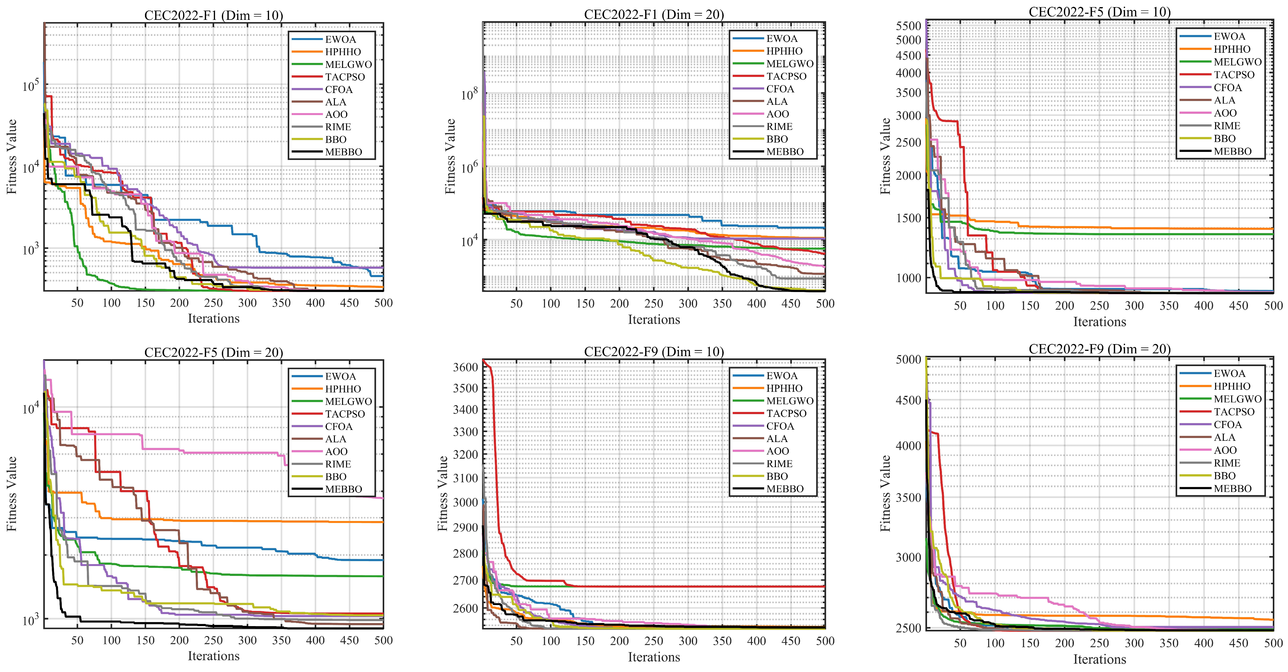
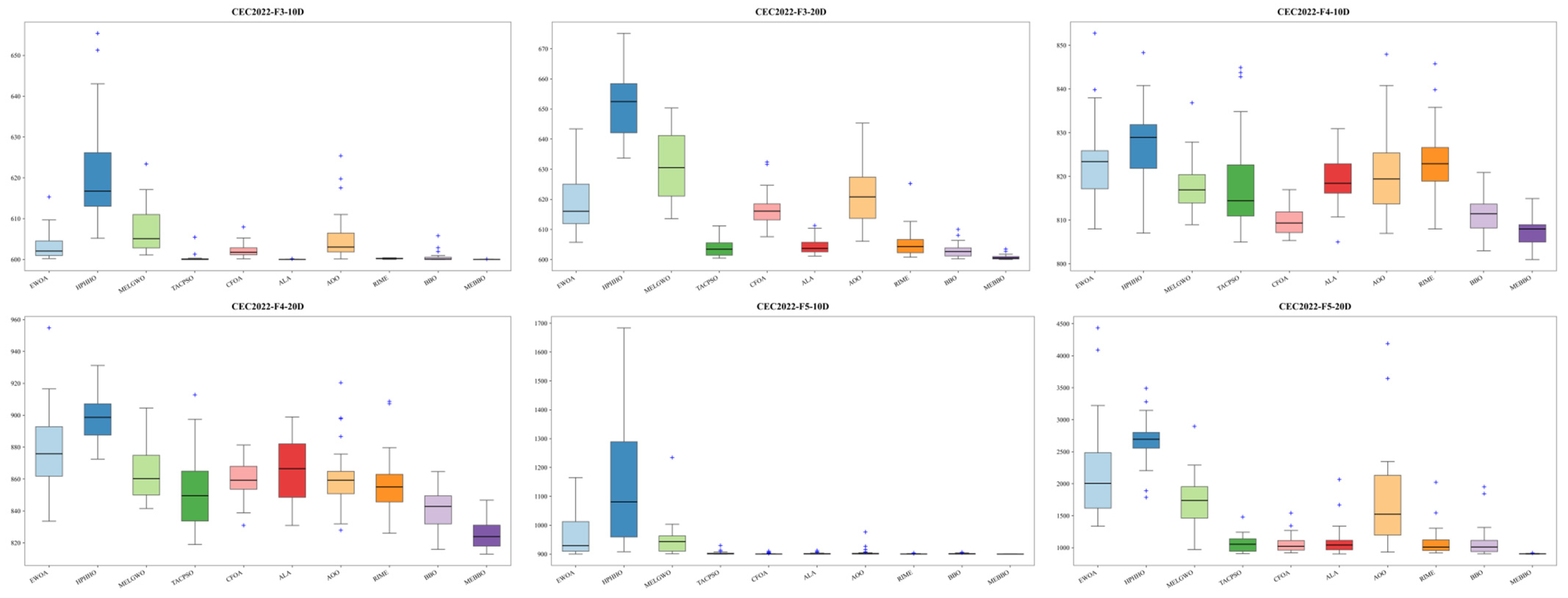
Figure 7 and Figure 8 present the convergence curves and boxplots of MEBBO on selected representative functions, respectively. As shown in Figure 7, after an initial rapid decline during the early iterations, MEBBO enters a relatively flat plateau phase before accelerating its convergence again. This indicates the algorithm’s ability to escape local optima during initial exploration and achieve efficient convergence near global optimal regions. Figure 8 shows that under varying dimensional conditions, MEBBO’s boxplots exhibit lower overall positions and narrower distribution ranges than those of the other algorithms, with smaller mean values and standard deviations—a pattern consistent with the numerical results presented in the corresponding result tables.

Table 17. Wilcoxon Rank-Sum Test results of MEBBO and 9 algorithms on the CEC 2022 (Dim = 10).

Algorithm	EWOA	HPHHO	MELGWO	TACPSO	CFOA	ALA	AOO	RIME	BBO
F1	3.0199 × 10−11	3.0199 × 10−11	3.3384 × 10−11	3.6897 × 10−11	3.0199 × 10−11	3.6897 × 10−11	3.0199 × 10−11	3.0199 × 10−11	9.8231 × 10−1
F2	1.5581 × 10−8	3.0199 × 10−11	3.1967 × 10−9	4.4196 × 10−7	2.2780 × 10−5	3.3259 × 10−11	4.5043 × 10−11	2.0338 × 10−9	2.5306 × 10−4
F3	3.0199 × 10−11	3.0199 × 10−11	3.0199 × 10−11	6.1452 × 10−2	3.0199 × 10−11	6.7350 × 10−1	3.0199 × 10−11	5.4941 × 10−11	2.1327 × 10−5
F4	1.0702 × 10−9	2.8716 × 10−10	5.0723 × 10−10	2.1526 × 10−6	9.8834 × 10−3	3.4742 × 10−10	9.7555 × 10−10	1.2057 × 10−10	3.9881 × 10−4
F5	1.7769 × 10−10	3.0199 × 10−11	3.0199 × 10−11	1.5169 × 10−3	2.6243 × 10−3	1.1058 × 10−4	4.1825 × 10−9	9.5207 × 10−4	8.1465 × 10−5
F6	3.8481 × 10−3	2.4327 × 10−5	5.2650 × 10−5	1.6813 × 10−4	7.0430 × 10−7	1.2212 × 10−2	5.9673 × 10−9	1.2477 × 10−4	7.6171 × 10−3
F7	2.7548 × 10−3	6.0104 × 10−8	1.6062 × 10−6	3.8710 × 10−1	1.3594 × 10−7	5.9969 × 10−1	1.1567 × 10−7	1.2235 × 10−1	1.2235 × 10−1
F8	3.4783 × 10−1	2.8314 × 10−8	3.5708 × 10−6	4.0330 × 10−3	3.0939 × 10−6	3.5547 × 10−1	1.1747 × 10−4	2.5101 × 10−2	2.4157 × 10−2
F9	3.0199 × 10−11	2.5721 × 10−7	1.1674 × 10−5	1.9350 × 10−6	1.5969 × 10−3	1.2118 × 10−12	2.6077 × 10−2	3.0199 × 10−11	3.0199 × 10−11
F10	6.3533 × 10−2	9.1171 × 10−1	3.5547 × 10−1	8.1874 × 10−1	1.3732 × 10−1	5.9969 × 10−1	9.3341 × 10−2	6.7350 × 10−1	1.9883 × 10−2
F11	6.6689 × 10−3	6.7650 × 10−5	1.6351 × 10−5	2.9041 × 10−1	6.7650 × 10−5	2.0058 × 10−4	3.0939 × 10−6	2.1540 × 10−6	3.1466 × 10−2
F12	7.5059 × 10−1	7.6183 × 10−1	3.5708 × 10−6	1.2592 × 10−1	1.4110 × 10−9	9.1950 × 10−9	5.0922 × 10−8	4.7138 × 10−4	5.7929 × 10−1

and

Table 18. Wilcoxon Rank-Sum Test results of MEBBO and 9 algorithms on the CEC 2022 (Dim = 20).

Algorithm	EWOA	HPHHO	MELGWO	TACPSO	CFOA	ALA	AOO	RIME	BBO
F1	3.0199 × 10−11	3.0199 × 10−11	3.0199 × 10−11	3.3384 × 10−11	3.0199 × 10−11	3.0199 × 10−11	6.0658 × 10−11	3.6897 × 10−11	9.7052 × 10−1
F2	8.1875 × 10−1	6.6955 × 10−11	3.1573 × 10−5	8.2357 × 10−2	7.3803 × 10−10	4.4272 × 10−3	2.4581 × 10−1	2.6433 × 10−1	9.5207 × 10−4
F3	3.0199 × 10−11	3.0199 × 10−11	3.0199 × 10−11	7.0881 × 10−8	3.0199 × 10−11	6.1210 × 10−10	3.0199 × 10−11	3.1967 × 10−9	2.8790 × 10−6
F4	1.6132 × 10−10	3.0199 × 10−11	4.9752 × 10−11	1.5964 × 10−7	1.2057 × 10−10	3.8202 × 10−10	1.9568 × 10−10	5.0723 × 10−10	2.1540 × 10−6
F5	3.0199 × 10−11	3.0199 × 10−11	3.0199 × 10−11	1.3289 × 10−10	3.0199 × 10−11	2.1544 × 10−10	3.0199 × 10−11	3.0199 × 10−11	3.4742 × 10−10
F6	8.6634 × 10−5	3.0199 × 10−11	3.3679 × 10−4	3.4029 × 10−1	6.1001 × 10−1	2.1544 × 10−10	1.9112 × 10−2	4.6159 × 10−10	3.0418 × 10−1
F7	2.9590 × 10−5	8.8910 × 10−10	4.6159 × 10−10	1.4423 × 10−3	3.9648 × 10−8	9.5332 × 10−7	7.1186 × 10−9	3.5923 × 10−5	2.7548 × 10−3
F8	6.3560 × 10−5	2.4386 × 10−9	4.5726 × 10−9	9.8231 × 10−1	1.3853 × 10−6	7.0430 × 10−7	1.4918 × 10−6	4.9426 × 10−5	7.9590 × 10−3
F9	1.4294 × 10−8	3.0199 × 10−11	5.6073 × 10−5	6.6272 × 10−1	3.0199 × 10−11	3.0199 × 10−11	8.1200 × 10−4	4.1825 × 10−9	6.6955 × 10−11
F10	1.3345 × 10−1	7.4827 × 10−2	4.0840 × 10−5	2.0621 × 10−1	7.3940 × 10−1	6.7650 × 10−5	1.9527 × 10−3	1.5367 × 10−1	7.2827 × 10−1
F11	1.5292 × 10−5	3.0199 × 10−11	6.5183 × 10−9	5.4933 × 10−1	3.8249 × 10−9	4.3764 × 10−1	1.1023 × 10−8	1.8500 × 10−8	1.5846 × 10−4
F12	9.9258 × 10−2	7.7725 × 10−9	6.0971 × 10−3	2.3985 × 10−1	1.2597 × 10−1	1.1058 × 10−4	3.2553 × 10−1	2.3399 × 10−1	6.6689 × 10−3

present the Wilcoxon rank-sum test results comparing MEBBO with nine benchmark algorithms under the 10-dimensional and 20-dimensional conditions on the CEC2022 test set. Overall, the majority of comparisons yielded p-values below 0.05, indicating statistically significant performance differences between MEBBO and most competing algorithms, which demonstrates that its optimization advantages are not attributable to random fluctuations. In the 10-dimensional dataset, MEBBO showed no statistically significant differences from MELGWO, CFOA, and AOO on only one function each, while showing no significant differences from HPHHO and RIME on merely two functions each. Under the 20-dimensional condition, MEBBO exhibited statistically significant differences from MELGWO across all 12 functions, and only one function for each of HPHHO and ALA remained statistically insignificant. These findings further confirm MEBBO’s robust and consistent statistical superiority on the CEC2022 test set.

The comparative results across multiple dimensions demonstrate that MEBBO’s significant advantage over most algorithms becomes even more pronounced as the problem dimensionality increases from 10 to 20. Notably, compared with the original BBO algorithm, MEBBO shows only three functions without statistically significant differences under both the 10-dimensional and 20-dimensional conditions, while all other functions reach statistically significant levels. This indicates that the proposed multi-strategy enhancement mechanism effectively improves overall algorithm performance. It should be emphasized that TACPSO exhibits strong competitiveness across both dimensions, with 5 and 7 functions showing no significant differences from MEBBO, respectively. Additionally, EWOA, ALA, CFOA, and RIME demonstrate comparable performance to MEBBO on certain functions. Overall, the Wilcoxon rank-sum test results provide statistical validation for MEBBO’s effectiveness, superiority, and robustness on the CEC2022 test set.

Table 19. Results of the Friedman average rank test on CEC2022.

Suites	CEC2022
Dimesions	10		20
Algorithm	Avg Rank	Overall Rank	Avg Rank	Overall Rank
EWOA	6.00	7	7.00	8
HPHHO	8.17	10	8.58	10
MELGWO	7.67	9	8.00	9
TACPSO	5.33	5	5.25	5
CFOA	4.33	3	5.42	6
ALA	3.58	2	4.42	3
AOO	6.58	8	6.50	7
RIME	5.67	6	4.83	4
BBO	4.67	4	3.08	2
MEBBO	3.00	1	1.92	1

presents the results of the Friedman test. MEBBO consistently ranked first overall across both dimensional conditions, with the Friedman rank values for the 10-dimensional and 20-dimensional datasets reported in Table 19. BBO maintained a stable second-place ranking across both dimensions, while TACPSO and RIME demonstrated strong performance, securing positions from third to fifth in the two-dimensional scenarios. In contrast, AOO, EWOA, and ALA exhibited moderate rankings, whereas HPHHO, MELGWO, and CFOA ranked relatively lower overall. 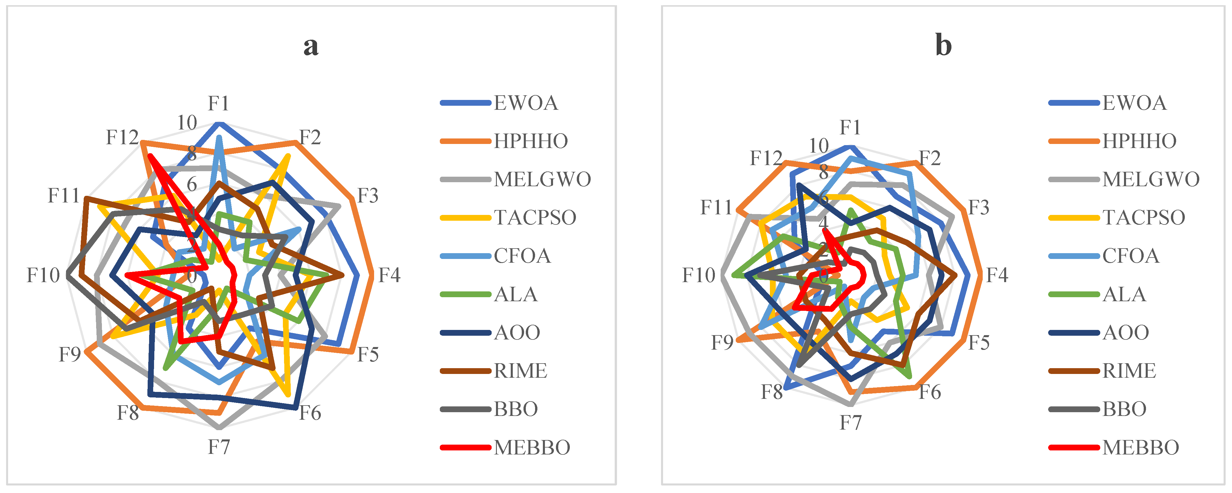Figure 9a and Figure 9b display radar charts of the Friedman test results for the 10-dimensional and 20-dimensional conditions, respectively. Consistent with the findings in Table 19, these visualizations clearly demonstrate MEBBO’s persistent position at the innermost location, further validating its highest comprehensive ranking.

5. Bankruptcy Prediction Problem

This section applies the proposed MEBBO algorithm to enterprise bankruptcy prediction. The purpose is to examine whether the optimization advantages observed in benchmark functions can be transferred to a practical financial classification task. Specifically, MEBBO is used to optimize the key parameters of KELM, and the resulting MEBBO-KELM model is evaluated using multiple classification metrics.

5.1. MEBBO-KELM

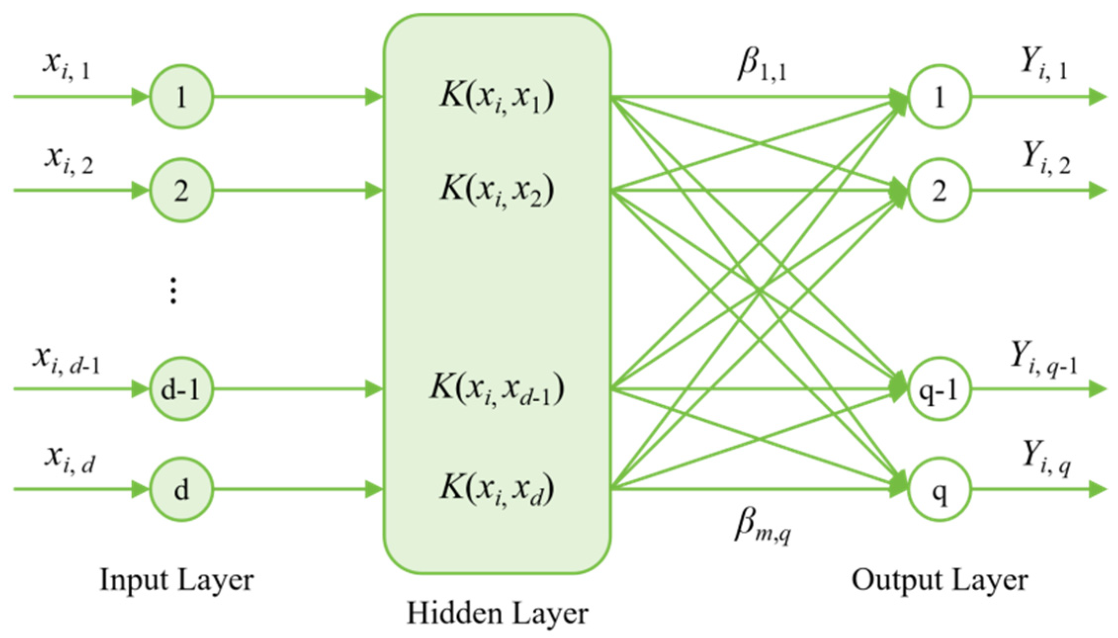
The Kernel Extreme Learning Machine (KELM) is an advanced learning model developed from the Extreme Learning Machine (ELM). Traditional ELMs randomly generate the connection weights and biases between the input and hidden layers and then solve the output weights using the least-squares method in a single step, offering advantages such as fast training speed and simple implementation. However, the random mapping approach may compromise model stability and generalization performance. To address this limitation, KELM introduces a kernel function mechanism that replaces explicit hidden-layer mappings with a kernel matrix, eliminating the uncertainties caused by manually setting the number of hidden-layer nodes and random parameters. With strong nonlinear modeling capabilities, rapid training efficiency, and excellent generalization performance, KELM is particularly effective for high-dimensional, nonlinear classification tasks with complex feature relationships, such as bankruptcy prediction. KELM inherits the fast learning property of ELM while using kernel mapping to improve nonlinear classification. However, its performance is highly sensitive to the penalty coefficient and kernel parameter; therefore, recent studies increasingly employ metaheuristic optimizers to tune these parameters in classification and bankruptcy prediction tasks [47,48]. The structure of KELM is shown in Figure 10.

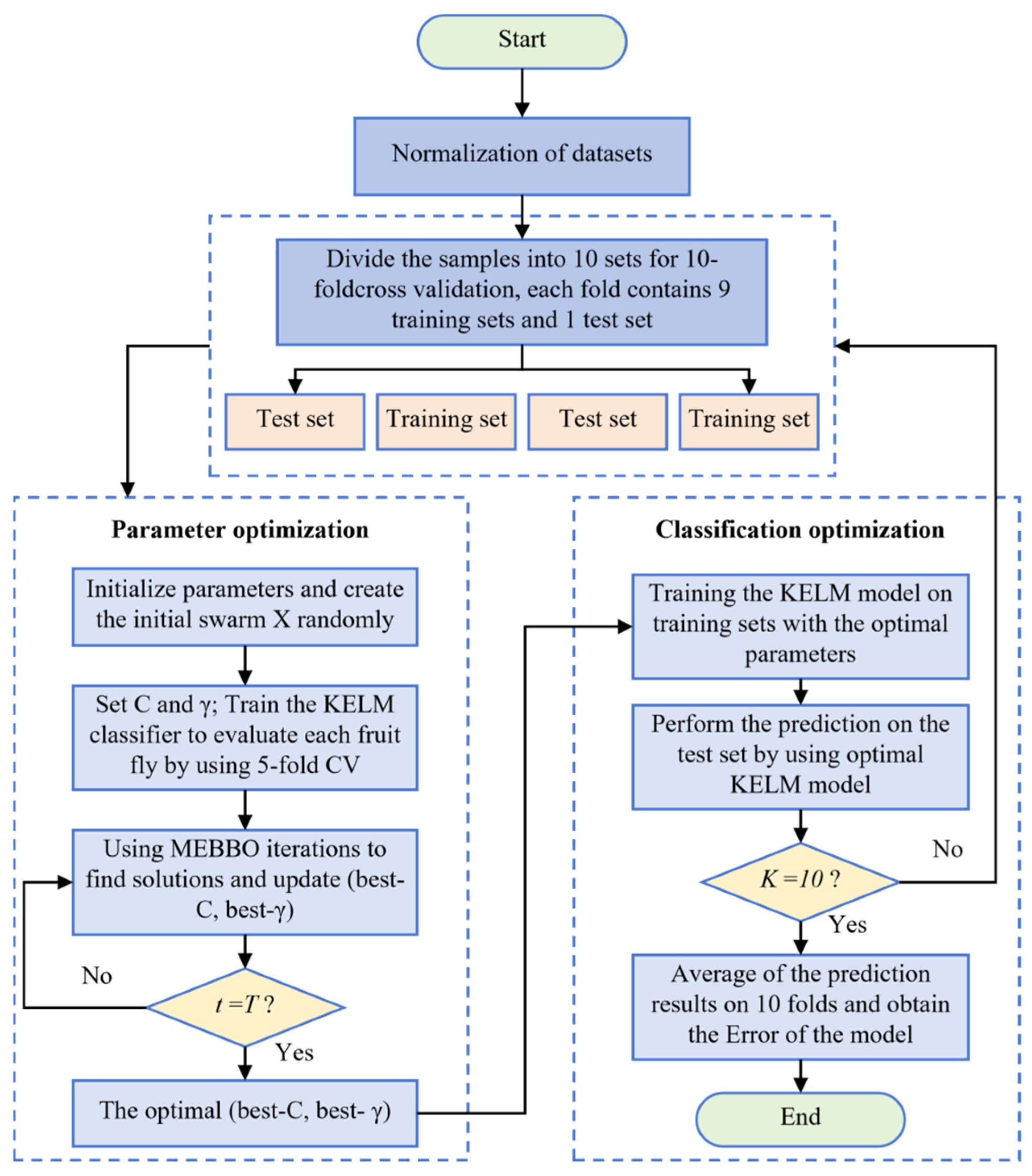
To further enhance the predictive accuracy and stability of KELM in bankruptcy forecasting, this study proposes the MEBBO-KELM model, which utilizes the MEBBO to optimize the key parameters of KELM. Specifically, MEBBO introduces three improvement strategies, elite pool-enhanced exploration, stochastic centroid reverse learning, and leader-guided boundary control, based on the original BBO algorithm. These innovations effectively increase population diversity, improve global search capabilities, and enhance convergence precision. Building upon this foundation, MEBBO automatically optimizes the kernel parameters and penalty coefficients in KELM, ensuring more rational parameter configurations and overcoming the limitations of traditional empirical settings or manual parameter tuning. Consequently, MEBBO-KELM effectively combines MEBBO’s global optimization advantages with KELM’s high-performance classification capabilities, providing enterprises with a more accurate and robust intelligent prediction model for bankruptcy forecasting. The workflow of the proposed MEBBO-KELM model is illustrated in Figure 11.

5.2. Experimental Setup

This study utilizes the Wieslaw dataset to validate the effectiveness of the MEBBO-KELM model in bankruptcy prediction. The dataset comprises 240 samples, each containing 30 feature indicators that primarily cover financial metrics and fundamental corporate information. Key characteristics include the debt-to-asset ratio, net profit margin, current ratio, cash flow, and operating revenue. These attributes comprehensively reflect a company’s financial health and operational performance, serving as crucial data sources for bankruptcy prediction research. Analysis of these indicators enables effective identification of potential financial crises and bankruptcy risks. The dataset is available for download on Kaggle.

Table 20. List of the features based on Wieslaw dataset and their definition.

NO	Features	NO	Features
C1	Cash/current liabilities	C16	Sales/receivables
C2	Cash/total assets	C17	Sales/total assets
C3	Current assets/current liabilities	C18	Sales/current assets
C4	Current assets/total assets	C19	365 $\times$ receivables/sales
C5	Working capital/total assets	C20	Sales/total assets
C6	Working capital/sales	C21	Liabilities/total income
C7	Sales/inventory	C22	Current liabilities/total income
C8	Sales/receivables	C23	Receivables/liabilities
C9	Net profit/total assets	C24	Net profit/sales
C10	Net profit/current assets	C25	Liabilities/total assets
C11	Net profit/sales	C26	Liabilities/equity
C12	Gross profit/sales	C27	Long-term liabilities/equity
C13	Net profit/liabilities	C28	Current liabilities/equity
C14	Net profit/equity	C29	EBIT/total assets
C15	Net profit/(equity + long term liabilities)	C30	Current assets/sales

summarizes detailed information about the Wieslaw dataset used in this study.

To evaluate the performance of the constructed MEBBO-KELM model in bankruptcy prediction, this study compares it with multiple existing optimization models, including EWOA-KELM, HPHHO-KELM, MELGWO-KELM, TACPSO-KELM, CFOA-KELM, ALA-KELM, AOO-KELM, RIME-KELM, and BBO-KELM. All optimization models uniformly set the population size to 30, with the problem dimensionality determined by the number of features in the dataset and the maximum number of iterations capped at 50 to ensure fairness and consistency in the comparative experiments. To guarantee the objectivity and reliability of the experimental results, tenfold cross-validation was employed to assess model classification performance. Specifically, the dataset was divided into 10 similarly sized subsets. In each experiment, 9 subsets were selected as the training set, while the remaining subset served as the test set. The process was repeated 10 times to ensure that each subset was used as a test set exactly once. The final evaluation metrics were calculated as the averages of the results from all 10 folds.

5.3. Data Preprocessing and Experimental Settings

Before constructing the bankruptcy prediction model, the Wieslaw dataset was preprocessed to ensure that all input variables were suitable for KELM-based classification. The original dataset was imported from an Excel file, where the first several columns were regarded as financial feature variables and the last column was used as the class label. The feature matrix and label vector were then separated. To meet the input requirement of the classification model, the class labels were converted into one-hot encoded vectors. In addition, since the original financial indicators may have different value ranges and scales, min–max normalization was applied to all feature variables, and each feature was linearly mapped into the interval [0, 1].

In the proposed MEBBO-KELM framework, MEBBO was used to optimize two key hyperparameters of KELM, namely the regularization parameter and the RBF kernel parameter. Therefore, the optimization dimension was set to 2. The lower and upper bounds of the two parameters were set to [1] and [20], respectively, and the radial basis function was adopted as the kernel function. The population size of each optimizer was set to 30, and the maximum number of iterations was set to 100. To ensure the fairness of comparison, all competing algorithms were configured with the same population size, maximum iteration number, search dimension, parameter boundaries, and fitness evaluation function. For comparative analysis, MEBBO-KELM was compared with nine optimizer-assisted KELM models, including EWOA-KELM, HPHHO-KELM, MELGWO-KELM, TACPSO-KELM, CFOA-KELM, ALA-KELM, AOO-KELM, RIME-KELM, and BBO-KELM. Each algorithm was independently executed 30 times to reduce the influence of randomness. In each run, the optimizer first searched for the optimal KELM hyperparameter combination, and then the obtained optimal parameters were used to evaluate the classification performance of KELM. The fitness function was defined based on the classification performance of KELM, and cross-validation was adopted during model evaluation to improve the reliability of the results.

5.4. Measures for Performance Evaluation

To comprehensively evaluate the classification performance of the proposed model in bankruptcy prediction tasks, this study selects seven evaluation metrics: accuracy (ACC), Matthews correlation coefficient (MCC), sensitivity, specificity, precision, recall, and F1 score. These metrics provide a systematic assessment of model performance across multiple dimensions—including overall classification accuracy, positive and negative sample recognition capability, and the balance of predictive results—thereby offering a more comprehensive reflection of the model’s effectiveness and robustness in bankruptcy prediction scenarios.

5.5. Experimental Results and Analysis

As shown in

Table 21. MEBBO-KELM Bankruptcy Prediction Results.

Algorithm	ACC Mean	MCC Mean	Sensitivity Mean	Specificity Mean	Precision Mean	Recall Mean	F1 Mean
EWOA	75.6264	0.5198	76.5404	74.7906	73.6725	76.5404	74.4886
HPHHO	75.9469	0.5259	76.5859	75.3825	73.9749	76.5859	74.6868
MELGWO	76.0430	0.5292	76.8081	75.3996	73.9915	76.8081	74.6723
TACPSO	76.7058	0.5418	77.4141	76.1090	74.7479	77.4141	75.4408
CFOA	76.2899	0.5328	76.7071	75.9594	74.5120	76.7071	75.0044
ALA	76.7167	0.5417	76.8838	76.5726	75.1567	76.8838	75.3636
AOO	76.2485	0.5326	76.9975	75.5791	74.4223	76.9975	75.0529
RIME	75.8265	0.5262	76.7803	75.0064	73.9484	76.7803	74.5760
BBO	74.8598	0.5064	75.7348	74.0919	72.8921	75.7348	73.5401
MEBBO	79.7578	0.6050	81.6288	78.1111	77.4726	81.6288	78.8504

, MEBBO-KELM achieved the best results across all evaluation metrics, demonstrating superior bankruptcy prediction performance. Its ACC, MCC, Sensitivity, Specificity, Precision, Recall, and F1 score reached 79.7578, 0.6050, 81.6288, 78.1111, 77.4726, 81.6288, and 78.8504, respectively, showing better performance than the other comparison algorithms in this dataset. This indicates its notable advantages in overall classification accuracy, positive and negative sample recognition capability, and comprehensive predictive performance. Among the comparison algorithms, TACPSO and ALA showed relatively strong results, ranking highly on metrics such as ACC, MCC, Specificity, and F1 score. In contrast, the original BBO performed relatively poorly, with ACC, MCC, and F1 score values of only 74.8598, 0.5064, and 73.5401, respectively. MEBBO achieved significant improvements over BBO across all metrics, particularly in key indicators including ACC, MCC, Recall, and F1 score. This demonstrates that the proposed multi-strategy enhancement mechanism effectively improves BBO’s global search capability and parameter optimization efficiency, thereby enhancing KELM’s classification performance. Overall, MEBBO-KELM exhibits strong effectiveness and robustness in the Wieslaw bankruptcy prediction task.

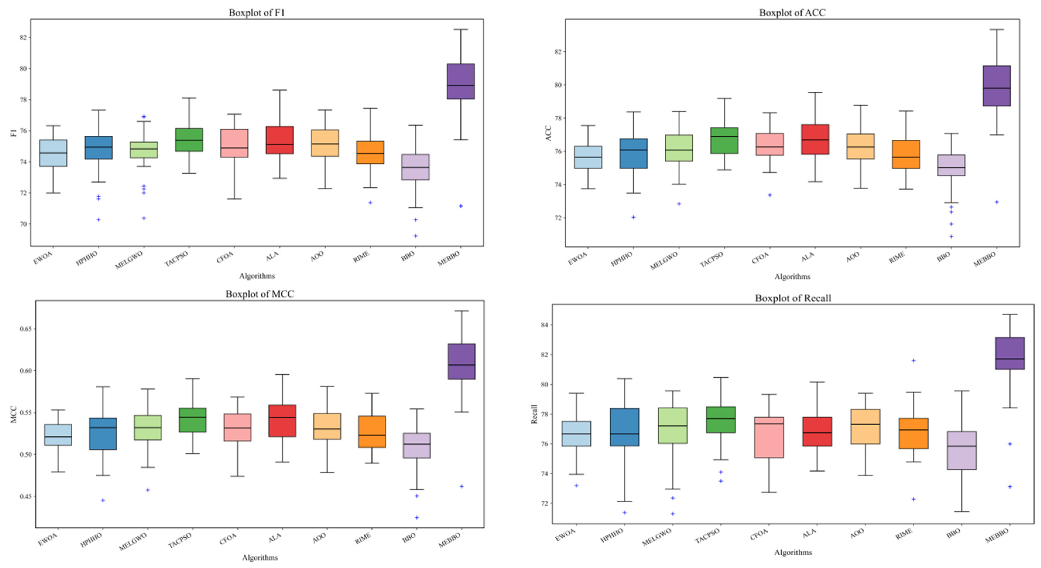
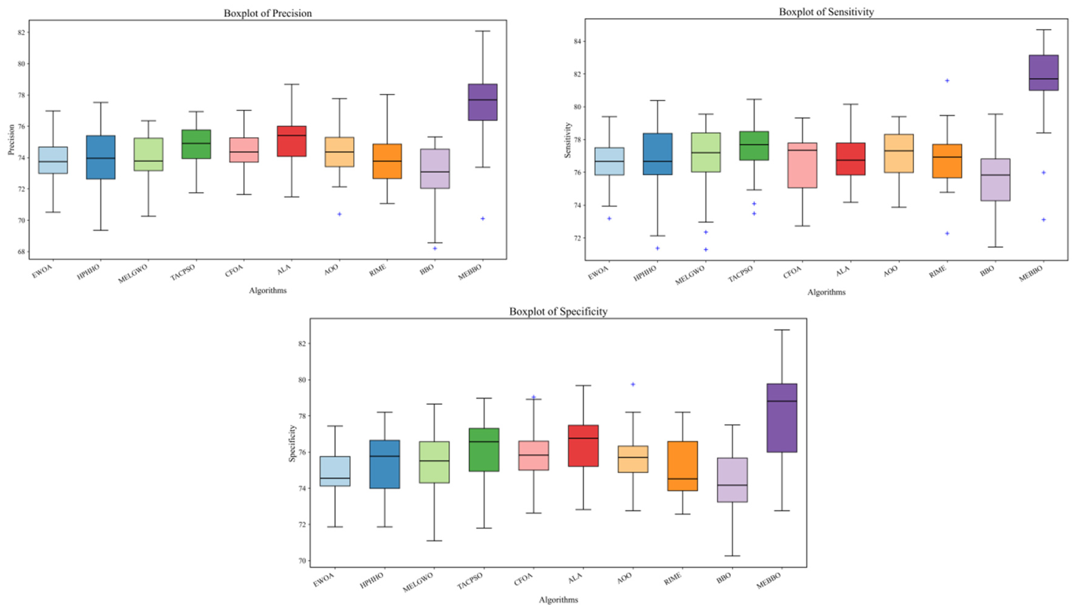
Figure 12 presents the boxplots of the prediction results for each model on the Wieslaw dataset. The plot further illustrates the distribution of prediction outcomes, demonstrating that the MEBBO-KELM model exhibits a more concentrated result distribution with fewer outliers, indicating higher stability and reliability in processing this dataset.

5.6. Generalization Analysis

To further examine the generalization ability of the proposed MEBBO-KELM model across different financial scenarios, this study additionally conducts bankruptcy prediction experiments on the German dataset. The same experimental settings and evaluation metrics are adopted as those used in the main bankruptcy prediction experiment, including ACC, MCC, Sensitivity, Specificity, Precision, Recall, and F1-score. The comparative results are reported in

Table 22. MEBBO-KELM Bankruptcy Prediction Results of German dataset.

Algorithm	ACC Mean	MCC Mean	Sensitivity Mean	Specificity Mean	Precision Mean	Recall Mean	F1 Mean
EWOA	76.7700	0.4128	89.0333	48.1556	80.0955	89.0333	84.2714
HPHHO	76.7600	0.4122	88.9857	48.2333	80.1095	88.9857	84.2666
MELGWO	76.8800	0.4156	89.0762	48.4222	80.1856	89.0762	84.3466
TACPSO	76.9433	0.4160	89.1857	48.3778	80.2113	89.1857	84.4085
CFOA	76.7767	0.4135	88.9286	48.4222	80.1662	88.9286	84.2629
ALA	76.9067	0.4156	89.1905	48.2444	80.1648	89.1905	84.3814
AOO	76.7267	0.4115	88.8286	48.4889	80.1787	88.8286	84.2285
RIME	76.9767	0.4170	89.3048	48.2111	80.1702	89.3048	84.4381
BBO	76.8367	0.4134	89.2286	47.9222	80.0618	89.2286	84.3451
MEBBO	76.9400	0.4158	89.3619	47.9556	80.1105	89.3619	84.4245

.

As shown in Table 22, all optimizer-assisted KELM models achieve relatively close performance on the German dataset, indicating that this dataset presents a relatively stable classification scenario for KELM-based models. Among all comparison methods, MEBBO-KELM obtains an ACC of 76.9400%, an MCC of 0.4158, a Sensitivity of 89.3619%, and an F1-score of 84.4245%. Although RIME-KELM achieves slightly higher ACC, MCC, and F1-score values, MEBBO-KELM obtains the highest Sensitivity among all models. This result suggests that the proposed model has a stronger ability to identify financially distressed firms, which is particularly important in bankruptcy prediction because failing to detect potential bankrupt firms may lead to substantial financial losses.

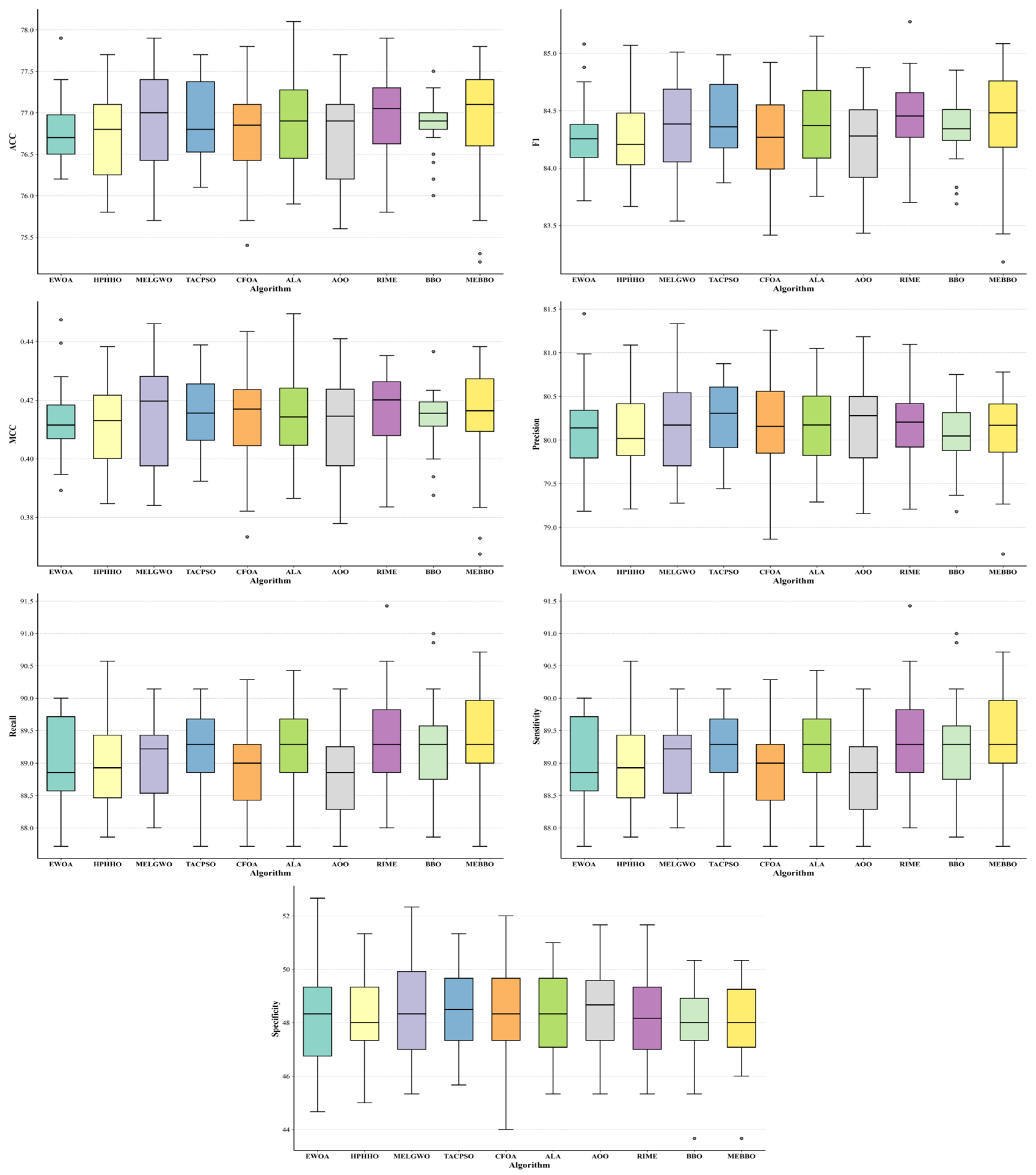
Figure 13 presents the box plots of the prediction results obtained by different optimizer-assisted KELM models on the German dataset. Overall, the distributions of most algorithms are relatively close, indicating that the German dataset is a stable but challenging classification scenario where performance differences among models are not highly pronounced. Nevertheless, MEBBO-KELM shows competitive and robust performance across most evaluation metrics. In terms of ACC and F1, MEBBO-KELM maintains a relatively high median value and an upper distribution comparable to the best-performing competitors, suggesting that the proposed model can achieve stable overall classification performance.

For Sensitivity and Recall, MEBBO-KELM exhibits a clear advantage, with its distribution concentrated at a relatively high level. This result indicates that MEBBO-KELM has a stronger ability to identify bankrupt firms, which is particularly important in bankruptcy prediction because misclassifying distressed firms may lead to higher financial risk. Although its Specificity is not the highest among all models, the overall box plot results show that MEBBO-KELM achieves a favorable balance between predictive accuracy, bankrupt-firm recognition, and result stability. Therefore, the results in Figure 13 further support the generalization ability of the proposed MEBBO-KELM model on an additional public bankruptcy dataset.

Overall, the results on the German dataset further demonstrate that MEBBO-KELM can maintain competitive predictive performance beyond the original bankruptcy dataset. Although its advantage is not dominant across all metrics, the model shows stable classification ability and strong bankrupt-firm recognition performance in a different financial dataset. Therefore, the additional experiment provides supplementary evidence for the generalization capability and practical applicability of the proposed MEBBO-KELM model in bankruptcy prediction tasks.

6. Discussion

This section further discusses the advantages, original contributions, and limitations of the proposed MEBBO in relation to similar improved metaheuristic algorithms. The main research gap addressed in this study is the limited adaptability of the original BBO in complex optimization problems involving high dimensionality, multimodality, nonlinear variable interactions, and boundary-sensitive search spaces. Although BBO provides a clear biologically inspired exploration–exploitation framework, its original search mechanism may suffer from unstable search guidance, insufficient population diversity, premature convergence, and inefficient boundary correction. These weaknesses become more evident when BBO is applied to complex benchmark functions and financial classification tasks such as bankruptcy prediction.

Compared with recent improved metaheuristic algorithms, the originality of MEBBO lies not in the simple combination of several common operators, but in the targeted reconstruction of the BBO search process. Specifically, the elite pool-enhanced exploration strategy improves the quality of search guidance by allowing individuals to learn from high-quality candidates rather than relying only on random learning objects. This process can be generally expressed as:

$$X_i^{t+1}=X_i^t+r\cdot \left(X_{elite}^t-X_i^t\right)$$

(16)

where $X_i^t$ denotes the current individual, $X_{elite}^t$ is an elite individual selected from the elite pool, and $r$ is a random coefficient. In addition, the stochastic centroid reverse learning strategy expands the search space from a population-distribution perspective. The stochastic centroid and its reverse candidate solution can be expressed as:

$$C^t={\displaystyle \frac{1}{m}}{\displaystyle \sum _{j=1}^m}{X}_j^t$$

(17)

$${\stackrel{-}{X}}_i^t=2C^t-X_i^t$$

(18)

Different from conventional opposition-based learning methods based mainly on fixed boundaries or the global best solution, this mechanism dynamically reflects the population distribution in each generation. The leader-guided boundary control strategy further transforms passive boundary truncation into an adaptive correction process guided by the current best individual. Therefore, the three strategies correspond respectively to three structural weaknesses of the original BBO: blind search guidance, insufficient ability to escape local optima, and inefficient boundary handling.

The experimental results further support the methodological contribution of MEBBO. On the CEC2017 and CEC2022 benchmark test suites, MEBBO shows competitive or superior performance across different function types, especially on multimodal, hybrid, and composite functions with complex landscapes and multiple local optima. This advantage can be attributed to the complementary effects of the three strategies: the elite pool improves search directionality, stochastic centroid reverse learning enhances population diversity, and leader-guided boundary control improves feasible-domain search stability. The Wilcoxon rank-sum test and Friedman test further confirm that the performance improvement of MEBBO is not limited to isolated functions but reflects stronger overall optimization robustness. Moreover, the ablation results indicate that each strategy contributes to the improvement of BBO from a different aspect, while the integrated MEBBO achieves the best overall performance.

From the application perspective, this study extends MEBBO to enterprise bankruptcy prediction by constructing the MEBBO-KELM model. Bankruptcy prediction is a typical nonlinear and high-dimensional financial classification problem, in which model performance is highly sensitive to parameter settings and data complexity. KELM has strong nonlinear classification ability and fast training speed, but its effectiveness depends heavily on the selection of kernel parameters and regularization coefficients. By using MEBBO to optimize these key parameters, MEBBO-KELM reduces the uncertainty caused by manual parameter tuning and improves classification performance. The empirical results show that MEBBO-KELM achieves competitive or superior performance on most evaluation metrics and shows particular advantages in bankrupt-firm identification, demonstrating its practical value in financial risk prediction.

Despite these advantages, MEBBO still has several limitations. First, the introduction of multiple enhancement strategies increases the structural complexity and computational cost of the algorithm compared with the original BBO. Second, its performance may still be affected by strategy-related parameters, such as the elite pool size, the frequency of reverse learning, and the boundary correction control mechanism. Third, the bankruptcy prediction experiment is conducted on a specific corporate bankruptcy dataset, so its generalizability across different countries, industries, time periods, and financial reporting environments should be interpreted with caution. Finally, the current MEBBO-KELM framework mainly focuses on parameter optimization and does not incorporate feature selection, although redundant or noisy financial indicators may affect prediction efficiency and model interpretability.

7. Conclusions and Future Works

This study proposes a Multi-Strategy Enhanced Beaver Behavior Optimizer (MEBBO) to address the limitations of the original BBO algorithm in solving complex optimization problems, including susceptibility to local optima, insufficient population diversity, and limited late-stage exploitation capabilities. Building upon the original BBO framework, three improvement strategies are introduced. First, an elite pool-enhanced exploration strategy leverages high-performing individuals to guide early-stage search expansion. Second, a stochastic centroid reverse learning strategy enhances population diversity and improves the algorithm’s ability to escape local optima. Third, a leader-guided boundary control strategy enables boundary-crossing individuals to re-enter the feasible domain under the guidance of the current best individual, thereby boosting search efficiency and solution quality. These three strategies work synergistically to significantly enhance the algorithm’s global search capability and local exploitation efficiency.

To validate the proposed method’s effectiveness, this study conducted comparative analyses between MEBBO and multiple advanced meta-heuristic algorithms on the CEC2017 and CEC2022 benchmark datasets. Experimental results demonstrate that MEBBO exhibits strong competitiveness in terms of both convergence accuracy and optimization performance, indicating its advantages in solving complex continuous optimization problems. Building on this foundation, we applied MEBBO to optimize the key parameters of kernel extreme learning machines (KELM) and constructed the MEBBO-KELM bankruptcy prediction model. Experimental results on the bankruptcy prediction datasets indicate that the proposed model achieves competitive or superior performance on most evaluation metrics, including ACC, MCC, Sensitivity, Specificity, Precision, Recall, and F1 score, and shows particular advantages in identifying bankrupt firms. These findings demonstrate that MEBBO effectively enhances KELM classification performance, thereby improving the accuracy and robustness of bankruptcy prediction outcomes.

Overall, the proposed MEBBO framework not only enriches research on BBO improvement but also provides novel insights into the application of meta-heuristic algorithms in bankruptcy prediction. Although the proposed MEBBO-KELM model shows promising performance in enterprise bankruptcy prediction, several directions remain worthy of further investigation. First, future studies can further improve the computational efficiency and parameter adaptability of MEBBO. Since the introduction of the elite pool, stochastic centroid reverse learning, and leader-guided boundary control increases the structural complexity of the algorithm, more lightweight or adaptive versions of MEBBO can be developed to reduce computational cost while maintaining optimization accuracy. In addition, adaptive parameter control mechanisms can be introduced to automatically adjust key strategy-related parameters, such as the elite pool size, the frequency of reverse learning, and the boundary correction intensity, so as to enhance the stability and generalization ability of the algorithm under different optimization scenarios.

Second, future research can extend the current MEBBO-KELM framework from single parameter optimization to joint feature selection and parameter optimization. In bankruptcy prediction, financial indicators often contain redundant, correlated, or noisy information, which may reduce prediction efficiency and weaken model interpretability. Therefore, a binary or multi-objective version of MEBBO can be designed to select informative financial indicators while optimizing KELM parameters. This extension would help reduce redundant input variables, improve computational efficiency, and provide more interpretable bankruptcy prediction results. Moreover, the current empirical analysis is based on one bankruptcy dataset and one main learning model. Future studies should validate the proposed framework on more bankruptcy datasets from different countries, industries, and time periods, and compare it with classical statistical models, such as logistic regression and discriminant analysis, as well as alternative machine learning models, such as support vector machines, random forests, gradient boosting methods, and deep neural networks. These additional comparisons would provide a more comprehensive evaluation of the robustness, applicability, and practical value of MEBBO in financial risk prediction.