Fast Feature Selection in Interval Data Using Rough Sets with Fuzzy Tolerance Relation-Based Hierarchical Approximations

Abstract

As a highly active research field, feature selection plays a critical role in multi-criteria decision making, hierarchical data analysis, and artificial intelligence. Rough set (RS) theory, presented by Pawlak, is a useful and important methodology for feature selection. Discernibility matrix-based and heuristic methods are two important rough set approaches for feature selection in interval-valued data. However, they still face significant computational challenges when dealing with high-dimensional and large-scale interval-valued data. To improve the efficiency of feature selection in an interval-valued decision system (IvDS), we construct a hierarchical approximation model and establish the corresponding theoretical results based on the fuzzy tolerance relation, which is symmetric and reflexive. Based on this model, we explore the order-preservation property of attribute significance in an IvDS and achieve attribute reduction on a gradually decreasing universe, which improves the efficiency of feature selection. Motivated by this idea, we develop two fast algorithms, named FFSDF and FFSCE. The proposed algorithms can achieve higher efficiency while preserving the same reduction results as the original feature selection algorithms. Finally, experiments are conducted on fifteen datasets to demonstrate that the proposed fast algorithms are more effective and efficient.

1. Introduction

As an important practical technique, feature selection [1,2,3,4] can identify necessary and crucial features from raw data. It has shown a great impact on different research fields. Rough set (RS) theory serves as a powerful theoretical tool for handling uncertain and incomplete information and has been widely applied in various practical fields, including decision analysis, medical diagnosis [5,6,7], and economic analysis [8,9]. Feature selection based on RS theory [10], also known as attribute reduction [11,12,13,14], is a powerful and meaningful technique to eliminate unnecessary or dispensable attributes in decision systems. So far, many feature selection methods based on RSs have been explored [15,16,17,18], such as generalized decision preservation [19], dependency degree preservation [20], and mutual information preservation [21]. In real-world problems, decision systems with interval values usually contain unneeded or redundant attributes, which will reduce the computational efficiency of algorithms. Therefore, feature selection based on RSs from an interval-valued decision system (IvDS) becomes necessary and crucial. Discernibility matrix (DM)-based and heuristic methods are widely used for feature selection in interval data.

A reduct in RS theory refers to a minimal feature subset that preserves the discriminative ability of the original IvDS. For a given IvDS, there commonly exist more than one reduct in practical applications. We can find all reducts of an IvDS by using DM-based methods. Leung et al. [22] granulated the universe by using the $\alpha$-tolerance relation and constructed the $\alpha$-DM to eliminate the unnecessary attributes from an IvDS. Aiming to derive simpler rules, Qian et al. [23] introduced a DM based on a dominance relation and its associated function in an IvDS. Yang et al. [24] defined a flexible binary relation in an IvDS, called the $\alpha$-dominance relation. On this basis, new DMs based on rough approximations were put forward to obtain all reducts from an IvDS. In a tolerance relation-based IvDS, any two objects in a class may not be similar to each other. To tackle this issue, Miao et al. [25] put forward $\alpha$-maximal definable sets to form approximations and established a new method to obtain reducts from an IvDS. Du et al. [26] constructed a matrix of approximate distribution to uncover the knowledge hidden in an inconsistent IvDS.

DM-based approaches are capable of identifying all reducts from an IvDS. However, such methods have been proven to be NP-hard and often computationally expensive in practical scenarios. To improve the time efficiency of feature selection from an IvDS, heuristic or greedy methods of feature selection in an IvDS have been proposed. Li et al. [27] introduced two indices to characterize the order relation in generalized systems with interval numbers (IV-OIFS). On the basis of this model, they further developed an algorithm for the reduction of an IV-OIFS. Wang et al. [28] presented a neighborhood radius via fuzzy sets and subsequently developed a new adaptive model of RSs. By exploring the relations between decision classes and attributes, they developed an efficient matrix-based reduction approach. A system combining interval numbers and multiple labels was proposed by Qin et al. [29]. Considering the relationships between different labels, an effective reduction technique was presented to select features in such a system. Unlike traditional RS reduction, which ranks attributes based on their significance, Xu et al. [30] adopted a preference-based approach to rank attributes and thereby identified the most important ones. Chen et al. [31] proposed three granularity measures and three conditional entropies using a three-way decision framework [32]. Based on these, they presented eight algorithms, seven of which outperform existing algorithms. Two dynamic algorithms [33] for IvDSs were proposed by employing the self-information method using fuzzy similarity relation. Dai et al. [34] first introduced inner and outer significance measures based on conditional entropy and developed two feature selection algorithms for interval data. Xu et al. [35] designed three greedy feature selection algorithms to remove the irrelevant attributes from electric power datasets. In a fuzzy ordered IvDS, Zhang et al. [36] put forward importance measures based on the belief function of evidence theory. EI-Bably et al. [5] proposed eight innovative types of initial neighborhoods, which can achieve higher classification accuracy compared with existing methods. The newly developed neighborhood rough set model provides a solid foundation and innovative insights for constructing new attribute significance measures and designing advanced feature selection algorithms.

Although heuristic feature selection methods in IvDSs are more efficient than DM-based ones, they still face significant computational challenges when dealing with high-dimensional and large-scale interval-valued data. To tackle this issue, we establish a hierarchical approximation model in an IvDS and study the relative theorems. Then, we investigate order-preservation properties in an IvDS. By using the strategy of order preservation of attribute significance measures, we develop two fast algorithms based on the dependency degree and Liang’s entropy. Finally, the experiments are conducted on eight UCI datasets to indicate that the proposed fast algorithms are effective and efficient in feature selection from an IvDS.

The primary contributions of this work are summarized as follows:

• Novel model. According to the monotonicity of positive regions regarding condition attributes, we establish a hierarchical approximation (HRA) model in an IvDS. With this model, positive regions at a finer granularity can be computed from those at a coarser granularity. Furthermore, theorems concerning the properties of the HRA model are established.
• Theoretical analyses. Based on the HRA model, the order preservation of attribute significance in an IvDS is investigated in this paper. Furthermore, we find that the sequence of attributes to be selected remains unchanged on a dwindling universe, which can reduce the computational time for feature selection.
• Efficient algorithms. By selecting the attribute with the maximum significance on the dwindling universe, we design two fast algorithms, named FFSDF and FFSCE, based on the dependency degree and Liang’s entropy.
• Comparative experiments. Experiments are conducted on fifteen UCI datasets to demonstrate that the proposed fast algorithms are significantly more efficient for feature selection in IvDSs.

For the convenience of discussion, our work is arranged as follows: Some fundamental concepts about RST in an IvDS are reviewed in Section 2. Hierarchical approximations are studied, and the relative theorems are also investigated in Section 3. To design fast feature selection algorithms in an IvDS, the order preservation of attribute significance measures is researched in Section 4. Two fast algorithms for feature selection (FFSDF and FFSCE) are developed based on the dependency degree and Liang’s conditional entropy in Section 5. Comparative experiments are conducted to verify that FFSDF and FFSCE are effective and efficient in Section 6. The conclusions and future works are presented in Section 7.

2. Preliminaries

In the theory of RSs, an interval-valued decision system (IvDS) [25,37,38] is a tabular representation of interval values, which can be formulated as $\mathcal{ID}=(O,AT=A\cup D,M_{a_s})$. The universe $O=\{o_1,o_2,\dots ,o_m\}$ is the collection of rows (objects), and $A=\{a_1,a_2,\dots ,a_n,d\}$ is a collection of columns (attributes). $AT$ is composed of two different parts: the first part is a condition attribute set $A=\{a_1,a_2,\dots ,a_n\}$, and the second part is a decision attribute set $D=\left\{d\right\}$. Decision attribute set D shows the class of each object in the universe. For $a_s\in A$, $V_{a_s}$ is the set of value domains of conditional attribute $a_s$. $M:O\times A\to V_{a_s}$ is a binary mapping from object–attribute pairs to attribute values. $a_s\left(o_i\right)$ represents the attribute value of object $o_i$ with respect to the attribute $a_s\left(o_i\right)$. In an IvDS, if $a_s\in A$, then $a_s\left(o_i\right)$ is an interval value; otherwise, $a_s\left(o_i\right)$ is a single value. For a given object $o_i$, an interval value regarding $a_s\in A$ is denoted by $a_s\left(o_i\right)=[l_i^s,u_i^s]$, where $l_i^s$ and $u_i^s$ are the lower bound (LB) and the upper bound (UB) of an interval value $a_s\left(o_i\right)$, respectively.

Table 1. An IvDS.

O	${\mathit{a}}_1$	${\mathit{a}}_2$	${\mathit{a}}_3$	${\mathit{a}}_4$	d
$o_1$	[3,7]	[0,6]	[1,5]	[2,8]	1
$o_2$	[2,6]	[3,9]	[3,7]	[1,5]	0
$o_3$	[2,5]	[2,8]	[2,6]	[0,6]	1
$o_4$	[4,7]	[0,6]	[1,5]	[0,6]	1
$o_5$	[2,6]	[3,9]	[3,7]	[2,8]	1
$o_6$	[2,6]	[1,7]	[3,7]	[3,9]	1
$o_7$	[1,4]	[0,6]	[1,5]	[1,5]	0
$o_8$	[3,5]	[2,8]	[2,6]	[3,7]	0
$o_9$	[2,7]	[2,8]	[3,7]	[3,7]	0
$o_{10}$	[1,5]	[0,6]	[1,5]	[1,5]	0

is a given IvDS, which contains four condition attributes $a_1,a_2,a_3$, and $a_4$ and one decision attribute $a_5$. The conditional attributes are interval-valued, while the decision attribute is single-valued.

It is well known that Jaccard similarity [39,40] is a classical and important measure for evaluating the similarity between two sets. Using the LB and UB of interval numbers, Jaccard similarity can be reformulated as follows.

Definition 1 

([39]).  Given an $\mathcal{ID}$, for $\forall o_i,o_j\in O,a_s\in A$, the similarity between $a_s\left(o_i\right)$ and $a_s\left(o_j\right)$ is defined as

$${\beta }_{ij}^s=\left\{\begin{array}{cc}0\hfill & [l_i^s,u_i^s]\cap [l_j^s,u_j^s]=\varnothing \hfill \\ {\displaystyle \frac{min\left\{\right|u_i^s-l_j^s|,|u_j^s-l_i^s\left|\right\}}{|max\{u_i^s,u_j^s\}-min\{l_i^s,l_j^s\}|}}\hfill & \mathit{otherwise},\hfill \end{array}\right.$$

where $|u_i^s-l_i^s|$ is the length of an interval number $a_s\left(o_i\right)=[l_i^s,u_i^s]$.

It can be seen that $0\le {\beta }_{ij}^s\le 1$. We can choose appropriate similarity measures according to practical requirements. If ${\beta }_{ij}^s=0$, the intersection of $a_s\left(o_i\right)=[l_i^s,u_i^s]$ and $a_s\left(o_j\right)=[l_j^s,u_j^s]$ is empty; then the two interval numbers are totally different, and $u_i^s\le l_j^s$, or $u_j^s\le l_i^s$. If ${\beta }_{ij}^s=1$, $a_s\left(o_i\right)=[l_i^s,u_i^s]$ is equal to $a_s\left(o_j\right)=[l_j^s,u_j^s]$; then the two interval numbers are the same interval number, $l_i^s=l_j^s$, and $u_i^s=u_j^s$. If $0<{\beta }_{ij}^s<1$, the intersection of $a_s\left(o_i\right)=[l_i^s,u_i^s]$ and $a_s\left(o_j\right)=[l_j^s,u_j^s]$ is not empty; then the two interval numbers have the same part, and $l_j^s<u_i^s$, or $l_i^s<u_j^s$.

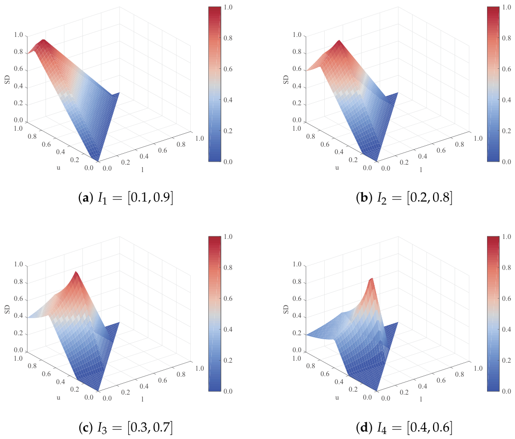
Figure 1 provides a graphical representation of the similarity degrees between different interval values and the given interval value. The l-axis represents the lower bound of an interval value, and the u-axis represents the upper bound. The SD-axis denotes the similarity degree between the interval value formed by the values on the l-axis and u-axis and a given interval value. For example, in Figure 1a, when the value of the l-axis is 0.1 and the value of the u-axis is 0.9, the similarity degree with respect to the given interval $[0.1,0.9]$ is 1, which corresponds to the maximum similarity degree. For any interval value $[l,u]$ constructed by the values on the l-axis and u-axis, we calculate its similarity degree with the given interval value. The smaller the similarity degree, the farther the SD value is away from the peak point of similarity.

Feature selection methods in classical RSs are mainly based on the equivalence relation. Nevertheless, universe classification based on the equivalence relation in an IvDS usually generates a large number of equivalence classes, which reduces the computational efficiency of feature selection and leads to incorrect reduction results. Hence, on the basis of the misclassification rates [22], Miao et al. [25] put forward the fuzzy tolerance relation as follows.

Definition 2 

([25]). Let $\mathcal{ID}=(O,A\cup D,M_{a_s})$ be an IvDS; for $\forall N\subseteq A$ and $o_i,o_j\in O$, $\beta \in [0,1]$ is a given similarity degree threshold, and the similarity relation with respect to O and N is defined as

$$S{R}_N^{(\beta ,O)}=\{(o_i,o_j)\in O\times O|{\beta }_{ij}^s\ge \beta ,\forall a_s\in N\}.$$

It is evident that $S{R}_N^{(\beta ,O)}$ is symmetric and reflexive, but $S{R}_N^{(\beta ,O)}$ may not be transitive. For $o_i,o_j\in O$, if the similarity between $o_i$ and $o_j$ is no less than a given value $\beta$, we say that $o_i$ is similar to $o_j$. Then, the objects $o_i$ and $o_j$ can be classified into one similarity class in the universe. The fuzzy similarity class of $o_i$ is defined as follows.

Definition 3 

([25]). Given an $\mathcal{ID}$, for $\forall N\subseteq A$, $o_i,o_j\in O$, and $\beta \in [0,1]$, $S{R}_N^{(\beta ,O)}$ is the fuzzy tolerance relation, and the fuzzy similarity class of $o_i$ regarding O and N is defined as

$$S{C}_N^{(\beta ,O)}\left(o_i\right)=\{o_j\in O|(o_i,o_j)\in S{R}_N^{(\beta ,O)}\}.$$

A cover on O determined by the fuzzy tolerance relation $S{R}_N^{(\beta ,O)}$ is

$$O/S{R}_N^{(\beta ,O)}=\{S{C}_N^{(\beta ,O)}\left(o_1\right),S{C}_N^{(\beta ,O)}\left(o_2\right),\dots ,S{C}_N^{(\beta ,O)}\left(o_m\right)\},$$

where $m=\left|O\right|$.

For $\forall N\subseteq A$, the lower and upper approximation sets (LAS and UAS) of $D_j$ in an IvDS are defined as follows.

$${\underline{APR}}_N^{(\beta ,O)}\left(D_j\right)=\{o_i\in O|S{C}_N^{(\beta ,O)}\left(o_i\right)\subseteq D_j\};$$

$${\overline{APR}}_N^{(\beta ,O)}\left(D_j\right)=\{o_i\in O|S{C}_N^{(\beta ,O)}\left(o_i\right)\cap D_j\ne \varnothing \}.$$

The LAS is a collection of $o_i\in O$ that satisfies $S{C}_N^{(\beta ,O)}\left(o_i\right)\subseteq D_j$, while the UAS is a collection of $o_i\in O$ such that $S{C}_N^{(\beta ,O)}\left(o_i\right)\cap D_j\ne \varnothing$.

Based on the LAS and UAS of $D_j$, the positive region (PR), boundary region (BR) and negative region (NR) of $D_j$ in an IvDS are defined as:

$$PO{S}_N^{(\beta ,O)}\left(D_j\right)={\underline{APR}}_N^{(\beta ,O)}\left(D_j\right),$$

$$BN{D}_N^{(\beta ,O)}\left(D_j\right)={\overline{APR}}_N^{(\beta ,O)}\left(D_j\right)-{\underline{APR}}_N^{(\beta ,O)}\left(D_j\right).$$

$$NE{G}_N^{(\beta ,O)}\left(D_j\right)=O-{\overline{APR}}_N^{(\beta ,O)}\left(D_j\right).$$

For $D_j\in O/D=\{D_1,D_2,\dots ,D_{|O/D|}\}$, the LAS and UAS of D are described as follows.

$${\underline{APR}}_N^{(\beta ,O)}\left(D\right)={\displaystyle \bigcup _{j=1}^{|O/D|}}{\underline{APR}}_N^{(\beta ,O)}\left(D_j\right),$$

$${\overline{APR}}_N^{(\beta ,O)}\left(D\right)={\displaystyle \bigcup _{j=1}^{|O/D|}}{\overline{APR}}_N^{(\beta ,O)}\left(D_j\right).$$

Then, positive, boundary and negative regions (PR, BR and NR) of D in an IvDS [25] are defined as follows.

$$PO{S}_N^{(\beta ,O)}\left(D\right)={\underline{APR}}_N^{(\beta ,O)}\left(D\right),$$

$$BN{D}_N^{(\beta ,O)}\left(D\right)={\overline{APR}}_N^{(\beta ,O)}\left(D\right)-{\underline{APR}}_N^{(\beta ,O)}\left(D\right).$$

$$NE{G}_N^{(\beta ,O)}\left(D\right)=O-{\overline{APR}}_N^{(\beta ,O)}\left(D\right).$$

For any $o_i\in S{C}_N^{(\beta ,O)}\left(o_i\right)\subseteq O$, there exists $D_j\in D$ such that $S{C}_N^{(\beta ,O)}\left(o_i\right)\cap D_j\ne \varnothing$; then, for any $o_i\in O$, it holds that $o_i\in {\overline{APR}}_N^{(\beta ,O)}\left(D\right)$. Therefore, $NE{G}_N^{(\beta ,O)}\left(D\right)=\varnothing$, i.e., ${\overline{APR}}_N^{(\beta ,O)}\left(D\right)=O$. Then, the following holds.

$$PO{S}_N^{(\beta ,O)}\left(D\right)\cup BN{D}_N^{(\beta ,O)}\left(D\right)={\overline{APR}}_N^{(\beta ,O)}\left(D\right)=O.$$

3. Hierarchical Approximations in Interval-Valued Decision Systems

3.1. A Novel Hierarchical Approximation Model

For a given IvDS, $N_1,N_2\subseteq A$, and $\beta \in [0,1]$, if there exist $S{C}_{N_1}^{(\beta ,O)}\left(o_i\right)\in O/S{R}_{N_1}^{(\beta ,O)}$ and $S{C}_{N_2}^{(\beta ,O)}\left(o_i\right)\in O/S{R}_{N_2}^{(\beta ,O)}$ such that $S{C}_{N_1}^{(\beta ,O)}\left(o_i\right)\supseteq S{C}_{N_2}^{(\beta ,O)}\left(o_i\right)$, where

$$\begin{array}{cc}\hfill O/S{R}_{N_1}^{(\beta ,O)}& =\{S{C}_{N_1}^{(\beta ,O)}\left(o_1\right),S{C}_{N_1}^{(\beta ,O)}\left(o_2\right),\dots ,S{C}_{N_1}^{(\beta ,O)}\left(o_{\left|O\right|}\right)\}\mathrm{and}\hfill \\ \hfill O/S{R}_{N_2}^{(\beta ,O)}& =\{S{C}_{N_2}^{(\beta ,O)}\left(o_1\right),S{C}_{N_2}^{(\beta ,O)}\left(o_2\right),\dots ,S{C}_{N_2}^{(\beta ,O)}\left(o_{\left|O\right|}\right)\}\hfill \end{array}$$

are covers with respect to $N_1$ and $N_2$, then $N_1⪰N_2$, where ⪰ is a hierarchical relation between $N_1$ and $N_2$. Granules derived by $N_1$ are coarser than granules derived by $N_2$; in other words, granules derived by $N_2$ are finer than granules derived by $N_1$. The relevant properties are presented as follows.

Proposition 1.  

Given an $\mathcal{ID}$, $\forall o_i\in O$, $N_1,N_2,N_3\subseteq A$, then we have that:

(1)   $N_1⪰N_1$, $N_2⪰N_2$, $N_3⪰N_3$ (reflexive);

(2)   If $N_1⪰N_2$ and $N_2⪰N_3$, then $N_1⪰N_3$ (transitive);

(3)   If $N_1⪰N_2$ and $N_2⪰N_1$, then $N_1=N_2$ (equal).

Proof. 

(1)   Since $S{C}_{N_1}^{(\beta ,O)}\left(o_i\right)=S{C}_{N_1}^{(\beta ,O)}\left(o_i\right)$, $S{C}_{N_2}^{(\beta ,O)}\left(o_i\right)=S{C}_{N_2}^{(\beta ,O)}\left(o_i\right)$ and $S{C}_{N_3}^{(\beta ,O)}\left(o_i\right)=S{C}_{N_3}^{(\beta ,O)}\left(o_i\right)$, then $S{C}_{N_1}^{(\beta ,O)}\left(o_i\right)\supseteq S{C}_{N_1}^{(\beta ,O)}\left(o_i\right)$, $S{C}_{N_2}^{(\beta ,O)}\left(o_i\right)\supseteq S{C}_{N_2}^{(\beta ,O)}\left(o_i\right)$ and $S{C}_{N_3}^{(\beta ,O)}\left(o_i\right)\supseteq S{C}_{N_3}^{(\beta ,O)}\left(o_i\right)$; thus $N_1⪰N_1$, $N_2⪰N_2$, and $N_3⪰N_3$.

(2)   If $N_1⪰N_2$ and $N_2⪰N_3$, we have $S{C}_{N_1}^{(\beta ,O)}\left(o_i\right)\supseteq S{C}_{N_2}^{(\beta ,O)}\left(o_i\right)$ and $S{C}_{N_2}^{(\beta ,O)}\left(o_i\right)\supseteq S{C}_{N_3}^{(\beta ,O)}\left(o_i\right)$; then $S{C}_{N_1}^{(\beta ,O)}\left(o_i\right)\supseteq S{C}_{N_3}^{(\beta ,O)}\left(o_i\right)$. Therefore, $N_1⪰N_3$.

(3)   If $N_1⪰N_2$ and $N_2⪰N_1$, then $S{C}_{N_1}^{(\beta ,O)}\left(o_i\right)\supseteq S{C}_{N_2}^{(\beta ,O)}\left(o_i\right)$, and $S{C}_{N_2}^{(\beta ,O)}\left(o_i\right)\supseteq S{C}_{N_1}^{(\beta ,O)}\left(o_i\right)$; it is easy to have $S{C}_{N_1}^{(\beta ,O)}\left(o_i\right)=S{C}_{N_2}^{(\beta ,O)}\left(o_i\right)$. Thus, $N_1=N_2$. This completes the proof.    □

From granular computing (GrC), each fuzzy similarity class forms a granule. The universe exhibits a hierarchical granular structure with the variation in attribute sets. The set inclusion relation of granules yields a partial order regarding coarseness and fineness.

From Proposition 1, hierarchical positive and boundary regions in an IvDS are defined as follows.

Definition 4.  

Given an $\mathcal{ID}$, $N_1,N_2,\dots N_i$ are the subsets of A, satisfying $N_1⪰N_2⪰\dots ⪰N_i$; the hierarchical positive and boundary regions (HPR and HBR) are defined as

$$PO{S}_{N_i}^{(\beta ,O)}\left(D\right)=PO{S}_{N_1}^{(\beta ,O)}\left(D\right)\cup {\displaystyle \bigcup _{j=2}^i}PO{S}_{N_j}^{(\beta ,BN{R}_{N_{j-1}}^{(\beta ,O)}\left(D\right))}\left(D\right),$$

$$BN{R}_{N_i}^{(\beta ,O)}\left(D\right)=BN{R}_{N_1}^{(\beta ,O)}\left(D\right)-{\displaystyle \bigcup _{j=2}^i}PO{S}_{N_j}^{(\beta ,BN{R}_{N_{j-1}}^{(\beta ,O)}\left(D\right))}\left(D\right).$$

Then, the proposition of HPR and HBR is described as follows.

Proposition 2.  

Given an $\mathcal{ID}$, if $N_1,N_2,\dots N_i$ are the subsets of A and $N_1⪰N_2⪰\dots ⪰N_i$, $\beta \in [0,1]$, then:

(1)   $|PO{S}_{N_i}^{(\beta ,O)}\left(D\right)|\ge |PO{S}_{N_{i-1}}^{(\beta ,O)}\left(D\right)|\ge \dots \ge |PO{S}_{N_1}^{(\beta ,O)}\left(D\right)|$;

(2)   $|BN{R}_{N_1}^{(\beta ,O)}\left(D\right)|\ge |BN{R}_{N_2}^{(\beta ,O)}\left(D\right)|\ge \dots \ge |BN{R}_{N_i}^{(\beta ,O)}\left(D\right)|$.

Hierarchical approximations (HRAs) regarding subset $N_i$ in an IvDS are defined as follows.

$${\underline{APR}}_{N_i}^{(\beta ,O)}\left(D\right)=PO{S}_{N_i}^{(\beta ,O)}\left(D\right);$$

$${\overline{APR}}_{N_i}^{(\beta ,O)}\left(D\right)=PO{S}_{N_i}^{(\beta ,O)}\left(D\right)\cup BN{R}_{N_i}^{(\beta ,O)}\left(D\right)=O.$$

Theorem 1.  

Given an $\mathcal{ID}$, $N_1,N_2,\dots N_i$ are the subsets of A and $N_1⪰N_2⪰\dots ⪰N_i$, $\beta \in [0,1]$. Then, we have

$$O^{\prime }-BN{R}_{N_i}^{(\beta ,O)}\left(D\right)=O^{\prime }-BN{R}_{N_i}^{(\beta ,O^{\prime })}\left(D\right),$$

(1)

where $O^{\prime }=BN{R}_{N_{i-1}}^{(\beta ,O)}\left(D\right)$.

Proof. 

According to Definition 4, if $O^{\prime }=BN{R}_{N_{i-1}}^{(\beta ,O)}\left(D\right)$, then we have

$$\begin{array}{c}\hfill O^{\prime }-BN{R}_{N_i}^{(\beta ,O)}\left(D\right)=PO{S}_{N_i}^{(\beta ,BN{R}_{N_{i-1}}^{(\beta ,O)}\left(D\right))}\left(D\right),\\ \hfill O^{\prime }-BN{R}_{N_i}^{(\beta ,O^{\prime })}\left(D\right)=PO{S}_{N_i}^{(\beta ,BN{R}_{N_{i-1}}^{(\beta ,O)}\left(D\right))}\left(D\right)\end{array}$$

Therefore, it follows that $O^{\prime }-BN{R}_{N_i}^{(\beta ,O)}\left(D\right)=O^{\prime }-BN{R}_{N_i}^{(\beta ,O^{\prime })}\left(D\right)$    □

Theorem 2.  

Given an $\mathcal{ID}$, $\forall o_i\in O$, $\beta \in [0,1]$, and $M\subseteq N\subseteq A$:

(1)   $S{R}_N^{(\beta ,O)}={\bigcap }_{a_s\in N}S{R}_{\left\{a_s\right\}}^{(\beta ,O)}$;

(2)   $S{C}_N^{(\beta ,O)}\left(o_i\right)\subseteq S{C}_M^{(\beta ,O)}\left(o_i\right)$.

Proof. 

(1)   For $\forall a_s\in N$, if $(o_i,o_j)\in {\bigcap }_{a_s\in N}S{R}_{\left\{a_s\right\}}^{(\beta ,O)}$, then objects $o_i$ and $o_j$ are similar regarding each attribute in N. Thus, we have $(o_i,o_j)\in S{R}_N^{(\beta ,O)}$. Then, we have ${\bigcap }_{a_s\in N}S{R}_{\left\{a_s\right\}}^{(\beta ,O)}\subseteq S{R}_N^{(\beta ,O)}$. According to Definition 2, if $(o_i,o_j)\in S{R}_N^{(\beta ,O)}$, $o_i$ and $o_j$ are similar for $\forall a_s\in N$; i.e., $(o_i,o_j)\in S{R}_{\left\{a_1\right\}}^{(\beta ,O)}$, $(o_i,o_j)\in S{R}_{\left\{a_2\right\}}^{(\beta ,O)}$, …, $(o_i,o_j)\in S{R}_{\left\{a_{\left|N\right|}\right\}}^{(\beta ,O)}$, then $(o_i,o_j)\in {\bigcap }_{a_s\in N}S{R}_{\left\{a_s\right\}}^{(\beta ,O)}$. Therefore, we have $S{R}_N^{(\beta ,O)}\subseteq {\bigcap }_{a_s\in N}S{R}_{\left\{a_s\right\}}^{(\beta ,O)}$. From the above discussion, we have that $S{R}_N^{(\beta ,O)}={\bigcap }_{a_s\in N}S{R}_{\left\{a_s\right\}}^{(\beta ,O)}$.

(2)   Assume that $S{C}_N^{(\beta ,O)}\left(o_i\right)\cancel{\subseteq }S{C}_M^{(\beta ,O)}\left(o_i\right)$; then $S{C}_M^{(\beta ,O)}\left(o_i\right)\subset S{C}_N^{(\beta ,O)}\left(o_i\right)$. Thus, there must exists $o_k\in O$ such that $(o_i,o_k)\in S{R}_N^{(\beta ,O)}$ and $(o_i,o_k)\notin S{R}_M^{(\beta ,O)}$. Then, there exists attribute t satisfying $t\in M$ and $t\notin N$. Then, $M⊈N$. This is contrary to $M\subseteq N\subseteq A$. Thus, $S{C}_N^{(\beta ,O)}\left(o_i\right)\subseteq S{C}_M^{(\beta ,O)}\left(o_i\right)$ holds.    □

If the upper or lower bound of interval values is missing, Jaccard similarity cannot measure the similarity between interval-valued data, and fuzzy similarity classes cannot be constructed. In this case, Theorem 2 no longer holds.

Since $N\subseteq N\cup \left\{a_s\right\}\subseteq A$, then we have $N⪰N\cup \left\{a_s\right\}⪰A$. Thus, Theorem 1 can be reformulated as follows.

Theorem 3.  

Given an $\mathcal{ID}$, $\forall N\subseteq A$, $a_s\in A-N$, and $\beta \in [0,1]$. Then, we have

$$BN{R}_N^{(\beta ,O)}\left(D\right)-BN{R}_{N\cup \left\{a_s\right\}}^{(\beta ,O)}\left(D\right)=O^{\prime }-BN{R}_{N\cup \left\{a_s\right\}}^{(\beta ,O^{\prime })}\left(D\right),$$

(2)

where $O^{\prime }=BN{R}_N^{(\beta ,O)}\left(D\right)$.

Proof. 

Since $N_i⪰N_{i-1}$, $N⪰N\cup \left\{a\right\}$. According to Theorem 1, we have $O^{\prime }-BN{R}_{N\cup \left\{a\right\}}^{(\beta ,O)}\left(D\right)=O^{\prime }-BN{R}_{N\cup \left\{a\right\}}^{(\beta ,O^{\prime })}\left(D\right)$, where $O^{\prime }=BN{R}_N^{(\beta ,O)}\left(D\right).$    □

Theorem 4.  

Given an $\mathcal{ID}$, $\forall N\subseteq A$, $a_s\in A-N$, and $\beta \in [0,1]$. Then, we have

$$|BN{R}_N^{(\beta ,O)}\left(D\right)-BN{R}_{N\cup \left\{a_s\right\}}^{(\beta ,O)}\left(D\right)|=|O-BN{R}_{N\cup \left\{a_s\right\}}^{(\beta ,O)}\left(D\right)|-|O-BN{R}_N^{(\beta ,O)}\left(D\right)|.$$

(3)

Proof. 

From Definition 4, we obtain $PO{S}_N^{(\beta ,O)}\left(D\right)\subseteq PO{S}_{N\cup \left\{a_s\right\}}^{(\beta ,O)}\left(D\right)$, that is, $O-BN{R}_N^{(\beta ,O)}\left(D\right)\subseteq O-BN{R}_{N\cup \left\{a_s\right\}}^{(\beta ,O)}\left(D\right)$. Hence,

$$\begin{array}{cc}\hfill & |BN{R}_N^{(\beta ,O)}\left(D\right)-BN{R}_{N\cup \left\{a_s\right\}}^{(\beta ,O)}\left(D\right)|\hfill \\ \hfill =& |(O-BN{R}_{N\cup \left\{a_s\right\}}^{(\beta ,O)}\left(D\right))-(O-BN{R}_N^{(\beta ,O)}\left(D\right))|\hfill \\ \hfill =& |O-BN{R}_N^{(\beta ,O)}\left(D\right)|-|O-BN{R}_{N\cup \left\{a_s\right\}}^{(\beta ,O)}\left(D\right)|.\hfill \end{array}$$

   □

Theorem 5.  

Given an $\mathcal{ID}$, $\forall N\subseteq A$, $o_i\in O$, $\beta \in [0,1]$, and $O^{\prime }=BN{R}_N^{(\beta ,O)}\left(D\right)$; then

$$\begin{array}{cc}\hfill & {\displaystyle \sum _{i=1}^{|O^{\prime }|}}\left(|S{C}_N^{(\beta ,O)}\left(o_i\right)|-|S{C}_N^{(\beta ,O)}\left(o_i\right)\cap S{C}_D^{(\beta ,O)}\left(o_i\right)|\right)\hfill \\ \hfill =& {\displaystyle \sum _{i=1}^{|O^{\prime }|}}\left(|S{C}_N^{(\beta ,O^{\prime })}\left(o_i\right)|-|S{C}_N^{(\beta ,O^{\prime })}\left(o_i\right)\cap S{C}_D^{(\beta ,O^{\prime })}\left(o_i\right)|\right).\hfill \end{array}$$

(4)

Proof. 

Assume that $o_j\in O-O^{\prime }$ and $o_j\in S{C}_N^{(\beta ,O)}\left(o_i\right)$. Since $S{R}_N^{(\beta ,O)}$ is symmetric, then $o_i\in S{C}_N^{(\beta ,O)}\left(o_j\right)$. Since $o_j\in O-O^{\prime }=AP{R}_N^{(\beta ,O)}\left(D\right)$, i.e., $o_j$ belongs to the positive region, then $S{C}_N^{(\beta ,O)}\left(o_j\right)\subseteq S{C}_D^{(\beta ,O)}\left(o_j\right)$. Thus, we have $o_i\in S{C}_D^{(\beta ,O)}\left(o_j\right)$.

As $S{C}_D^{(\beta ,O)}\left(o_j\right)$ is an equivalence class, we have $S{C}_D^{(\beta ,O)}\left(o_i\right)=S{C}_D^{(\beta ,O)}\left(o_j\right)$. Hence, $o_j\in S{C}_D^{(\beta ,O)}\left(o_i\right)$. Since $o_j\in S{C}_N^{(\beta ,O)}\left(o_i\right)$ and $o_j\in S{C}_D^{(\beta ,O)}\left(o_i\right)$, we have $o_j\in S{C}_N^{(\beta ,O)}\left(o_i\right)\cap S{C}_D^{(\beta ,O)}\left(o_i\right)$.

If $S=\left\{o_j\right|o_j\in O-O^{\prime }\}$, then

$$\begin{array}{cc}\hfill & S{C}_N^{(\beta ,O)}\left(o_i\right)-S{C}_N^{(\beta ,O)}\left(o_i\right)\cap S{C}_D^{(\beta ,O)}\left(o_i\right)\hfill \\ \hfill =& (S{C}_N^{(\beta ,O)}\left(o_i\right)-S)-(S{C}_N^{(\beta ,O)}\left(o_i\right)\cap S{C}_D^{(\beta ,O)}\left(o_i\right)-S)\hfill \\ \hfill =& \left(S{C}_N^{(\beta ,O-S)}\left(o_i\right)\right)-(S{C}_N^{(\beta ,O-S)}\left(o_i\right)\cap S{C}_D^{(\beta ,O-S)}\left(o_i\right))\hfill \\ \hfill =& S{C}_N^{(\beta ,O^{\prime })}\left(o_i\right)-(S{C}_N^{(\beta ,O^{\prime })}\left(o_i\right)\cap S{C}_D^{(\beta ,O^{\prime })}\left(o_i\right)).\hfill \end{array}$$

Since

$$\begin{array}{cc}\hfill & S{C}_N^{(\beta ,O)}\left(o_i\right)\cap S{C}_D^{(\beta ,O)}\left(o_i\right)\subseteq S{C}_N^{(\beta ,O)}\left(o_i\right)\mathrm{and}\hfill \\ \hfill & S{C}_N^{(\beta ,O^{\prime })}\left(o_i\right)\cap S{C}_D^{(\beta ,O^{\prime })}\left(o_i\right)\subseteq S{C}_N^{(\beta ,O^{\prime })}\left(o_i\right),\hfill \end{array}$$

we have

$$\begin{array}{cc}\hfill & {\displaystyle \sum _{i=1}^{|O^{\prime }|}}\left(\right|S{C}_N^{(\beta ,O)}\left(o_i\right)|-|S{C}_N^{(\beta ,O)}\left(o_i\right)\cap S{C}_D^{(\beta ,O)}\left(o_i\right)\left|\right)\hfill \\ \hfill =& {\displaystyle \sum _{i=1}^{|O^{\prime }|}}\left(\right|S{C}_N^{(\beta ,O^{\prime })}\left(o_i\right)|-|S{C}_N^{(\beta ,O^{\prime })}\left(o_i\right)\cap S{C}_D^{(\beta ,O^{\prime })}\left(o_i\right)\left|\right).\hfill \end{array}$$

   □

Theorem 6.  

Given an $\mathcal{ID}$, $\forall N\subseteq A$, $o_i\in O$, $\beta \in [0,1]$, and $O^{\prime }=BN{R}_N^{(\beta ,O)}\left(D\right)$; then

$$\begin{array}{cc}\hfill & {\displaystyle \sum _{i=1}^{\left|O\right|}}\left(|S{C}_N^{(\beta ,O)}\left(o_i\right)|-|S{C}_N^{(\beta ,O)}\left(o_i\right)\cap S{C}_D^{(\beta ,O)}\left(o_i\right)|\right)\hfill \\ \hfill =& {\displaystyle \sum _{i=1}^{|O^{\prime }|}}\left(|S{C}_N^{(\beta ,O^{\prime })}\left(o_i\right)|-|S{C}_N^{(\beta ,O^{\prime })}\left(o_i\right)\cap S{C}_D^{(\beta ,O^{\prime })}\left(o_i\right)|\right).\hfill \end{array}$$

(5)

Proof. 

If $o_i\in BN{R}_N^{(\beta ,O)}\left(D\right)$, $1\le i\le |O^{\prime }|$, then $o_i\in PO{S}_N^{(\beta ,O)}\left(D\right)$, $|O^{\prime }|+1\le i\le |O|$. Therefore,

$$\begin{array}{cc}\hfill & {\displaystyle \sum _{i=1}^{\left|O\right|}}\left(\right|S{C}_N^{(\beta ,O)}\left(o_i\right)|-|S{C}_N^{(\beta ,O)}\left(o_i\right)\cap S{C}_D^{(\beta ,O)}\left(o_i\right)\left|\right)\hfill \\ \hfill =& {\displaystyle \sum _{i=1}^{|O^{\prime }|}}\left(\right|S{C}_N^{(\beta ,O)}\left(o_i\right)|-|S{C}_N^{(\beta ,O)}\left(o_i\right)\cap S{C}_D^{(\beta ,O)}\left(o_i\right)\left|\right)+\hfill \\ \hfill & \sum _{i=|O^{\prime }|+1}^{\left|O\right|}\left(\right|S{C}_N^{(\beta ,O)}\left(o_i\right)|-|S{C}_N^{(\beta ,O)}\left(o_i\right)\cap S{C}_D^{(\beta ,O)}\left(o_i\right)\left|\right)\hfill \end{array}$$

For $o_i\in O-O^{\prime }=PO{S}_N^{(\beta ,O)}\left(D\right)$, we have

$$\begin{array}{c}\hfill S{C}_N^{(\beta ,O)}\left(o_i\right)=S{C}_N^{(\beta ,O)}\left(o_i\right)\cap S{C}_D^{(\beta ,O)}\left(o_i\right).\end{array}$$

Hence,

$$\begin{array}{c}\hfill \sum _{i=|O^{\prime }|+1}^{\left|O\right|}\left(\right|S{C}_N^{(\beta ,O)}\left(o_i\right)|-|S{C}_N^{(\beta ,O)}\left(o_i\right)\cap S{C}_D^{(\beta ,O)}\left(o_i\right)\left|\right)=0.\end{array}$$

According to Theorem 5, we have

$$\begin{array}{cc}\hfill & {\displaystyle \sum _{i=1}^{\left|O\right|}}\left(\right|S{C}_N^{(\beta ,O)}\left(o_i\right)|-|S{C}_N^{(\beta ,O)}\left(o_i\right)\cap S{C}_D^{(\beta ,O)}\left(o_i\right)\left|\right)\hfill \\ \hfill =& {\displaystyle \sum _{i=1}^{|O^{\prime }|}}\left(\right|S{C}_N^{(\beta ,O)}\left(o_i\right)|-|S{C}_N^{(\beta ,O)}\left(o_i\right)\cap S{C}_D^{(\beta ,O)}\left(o_i\right)\left|\right)+0\hfill \\ \hfill =& {\displaystyle \sum _{i=1}^{|O^{\prime }|}}\left(\right|S{C}_N^{(\beta ,O)}\left(o_i\right)|-|S{C}_N^{(\beta ,O)}\left(o_i\right)\cap S{C}_D^{(\beta ,O)}\left(o_i\right)\left|\right).\hfill \end{array}$$

Therefore, it can be concluded that

$$\begin{array}{cc}\hfill & {\displaystyle \sum _{i=1}^{\left|O\right|}}\left(\right|S{C}_N^{(\beta ,O)}\left(o_i\right)|-|S{C}_N^{(\beta ,O)}\left(o_i\right)\cap S{C}_D^{(\beta ,O)}\left(o_i\right)\left|\right)\hfill \\ \hfill =& {\displaystyle \sum _{i=1}^{|O^{\prime }|}}\left(\right|S{C}_N^{(\beta ,O^{\prime })}\left(o_i\right)|-|S{C}_N^{(\beta ,O^{\prime })}\left(o_i\right)\cap S{C}_D^{(\beta ,O^{\prime })}\left(o_i\right)|.\hfill \end{array}$$

   □

3.2. Discussion on the Hierarchical Approximation Model

Neighborhood rough sets, covering rough sets, and tolerance relation-based rough sets are important extended models in rough set theory. Numerous scholars have made substantial achievements in these research fields. The proposed HRA model is compared in detail with the three existing models, as listed in

Table 2. Comparison of four rough set models.

	Neighborhood Rough Set Model (NRS)	Covering Rough Set Model (CRS)	Tolerance Relation Rough Set Model (TRS)	Hierarchical Approximations Rough Set Model (HRA)
Data Type Processed	Continuous real-valued data	Discrete symbolic data, data with overlapping classifications	Single-valued discrete data, incomplete data with missing values, set-valued data	Interval-valued data, interval-valued decision system
Source of Uncertainty	Continuous values, measurement noise, fuzzy boundaries	Overlapping subsets of the universe	Missing attribute values, set-valued data	Interval range of attributes, uncertainty caused by interval overlap
Relation Construction Method	Distance measurement + neighborhood radius $\delta$, satisfying distance $d(x,y)\le \delta$	Covering family of universe subsets, neighborhood relation induced by covering blocks	Tolerance defined if attribute values are equal or missing values exist	Tolerance determined by calculating interval similarity + similarity degree threshold $\theta$
Basic Granular Structure	$\delta$-Neighborhood granule $N_{\delta }\left(x\right)$	Covering neighborhood $N\left(x\right)$	Single-valued tolerance class $R\left(x\right)$	Fuzzy similarity class $S{C}_N^{(\beta ,O)}\left(x\right)$
Reflexivity	Satisfied	Satisfied	Satisfied	Satisfied
Symmetry	Depends on the symmetry of the distance metric	Satisfied	Satisfied	Satisfied
Transitivity	Not satisfied	Not satisfied	Not satisfied	Not satisfied
Rough Approximation	Rough approximation based on single granular level	Rough approximation based on single granular level	Rough approximation based on single granular level	Rough approximation based on multiple granular levels
Core Parameters	Neighborhood radius $\delta$	No numerical threshold	No numerical threshold	Similarity degree threshold $\beta \in [0,1]$
Discretization Requirement	No discretization required; direct processing of continuous values	Requires discretization	Requires discretization	Compatible with interval values; no discretization required

. The proposed HRA model has the following advantages: (1) HRA can directly process interval-valued data without discretization and completely preserve interval-valued information. (2) The hierarchical approximation of interval values reveals the relationship between rough approximations over different attribute sets (i.e., coarse-grained and fine-grained granular layers). Based on this relationship, fast algorithms for interval-valued feature selection can be proposed.

4. Preservation of the Order of Attribute Significance

In this section, we explore the preservation of the order of attribute significance. On this basis, the sequence of attributes need to be selected is unchanged on a dwindling universe. We recall two important measures of attributes in RSs, i.e., dependency function and Liang’s conditional entropy. The dependency function in an IvDS [25,35,37] is expressed as follows.

Definition 5  

([35]). Given an $\mathcal{ID}$, $\forall N\subseteq A$, $\beta \in [0,1]$, the dependency function of D regarding N is given as follows.

$${\gamma }_N^{(\beta ,O)}\left(D\right)={\displaystyle \frac{|{\underline{APR}}_N^{(\beta ,O)}\left(D\right)|}{|{\overline{APR}}_N^{(\beta ,O)}\left(D\right)|}}={\displaystyle \frac{|PO{S}_N^{(\beta ,O)}\left(D\right)|}{\left|O\right|}},$$

(6)

where $\left|S\right|$ denotes the number of elements in S.

If ${\gamma }_N^{(\beta ,O)}\left(D\right)=1$, an IvDS is consistent; otherwise, it is inconsistent. Liang et al. [41] originally introduced conditional entropy, which differs from Shannon entropy. For an IvDS, Liang’s conditional entropy is given as follows.

Definition 6.  

Given an $\mathcal{ID}$, $\forall N\subseteq A$ and $\beta \in [0,1]$, $O/S{R}_N^{(\beta ,O)}=\{S{C}_N^{(\beta ,O)}\left(o_1\right),S{C}_N^{(\beta ,O)}\left(o_2\right),\dots ,S{C}_N^{(\beta ,O)}\left(o_m\right)\}$ and $O/S{R}_D^{(\beta ,O)}=\{S{C}_D^{(\beta ,O)}\left(o_1\right),S{C}_D^{(\beta ,O)}\left(o_2\right),\dots ,S{C}_D^{(\beta ,O)}\left(o_m\right)\}$ are classifications induced by N and D. Liang’s conditional entropy of D with respect to N is defined as follows.

$${\mu }_N^{(\beta ,O)}\left(D\right)={\displaystyle \frac{1}{{\left|O\right|}^2}}{\displaystyle \sum _{i=1}^m}\left(\right|S{C}_N^{(\beta ,O)}\left(o_i\right)|-|S{C}_N^{(\beta ,O)}\left(o_i\right)\cap S{C}_D^{(\beta ,O)}\left(o_i\right)\left|\right).$$

(7)

If Liang’s entropy equals zero, then an IvDS is certain. Otherwise, an IvDS is uncertain. In an uncertain IvDS, $0<{\mu }_N^{(\beta ,O)}\left(D\right)<1$. The greater the value of Liang’s entropy is, the larger the uncertainty of an IvDS is.

Based on Definitions 5 and 6, we obtain the following propositions.

Proposition 3.  

Given an $\mathcal{ID}$, for $\forall N_1,N_2\subseteq A$ and ${\beta }_1,{\beta }_2\in [0,1]$, we have that:

(1)   If $N_1⪰N_2$, then ${\gamma }_{N_2}^{({\beta }_1,O)}\left(D\right)\ge {\gamma }_{N_1}^{({\beta }_1,O)}\left(D\right)$;

(2)   If ${\beta }_1\ge {\beta }_2$, then ${\gamma }_{N_1}^{({\beta }_1,O)}\left(D\right)\ge {\gamma }_{N_1}^{({\beta }_2,O)}\left(D\right)$;

(3)   If $N_1⪰N_2$, then ${\mu }_{N_1}^{({\beta }_1,O)}\left(D\right)\ge {\mu }_{N_2}^{({\beta }_1,O)}\left(D\right)$;

(4)   If ${\beta }_1\ge {\beta }_2$, then ${\mu }_{N_1}^{({\beta }_2,O)}\left(D\right)\ge {\mu }_{N_1}^{({\beta }_1,O)}\left(D\right)$.

Proof. 

(1)   According to the definition of LAS, then

$$\begin{array}{c}\hfill {\underline{APR}}_N^{(\beta ,O)}\left(D\right)={\displaystyle \bigcup _{j=1}^{|O/D|}}{\underline{APR}}_N^{(\beta ,O)}\left(D_j\right)={\displaystyle \bigcup _{j=1}^{|O/D|}}\{o_i\in O|S{C}_N^{(\beta ,O)}\left(o_i\right)\subseteq D_j\}.\end{array}$$

If $N_1⪰N_2$, that is, $S{C}_{N_2}^{(\beta ,O)}\left(o_i\right)\subseteq S{C}_{N_1}^{(\beta ,O)}\left(o_i\right)$, then ${\underline{APR}}_{N_1}^{(\beta ,O)}\left(D\right)\subseteq {\underline{APR}}_{N_2}^{(\beta ,O)}\left(D\right)$. Therefore, $|{\underline{APR}}_{N_1}^{(\beta ,O)}\left(D\right)|\le |{\underline{APR}}_{N_2}^{(\beta ,O)}\left(D\right)|$. Then, we have

$$\begin{array}{c}\hfill {\gamma }_{N_1}^{(\beta ,O)}\left(D\right)={\displaystyle \frac{|{\underline{APR}}_{N_1}^{(\beta ,O)}\left(D\right)|}{\left|O\right|}}\le {\gamma }_{N_2}^{(\beta ,O)}\left(D\right)={\displaystyle \frac{|{\underline{APR}}_{N_2}^{(\beta ,O)}\left(D\right)|}{\left|O\right|}}.\end{array}$$

(2)   According to the definition of LAS, then

$$\begin{array}{c}\hfill {\underline{APR}}_N^{(\beta ,O)}\left(D\right)={\displaystyle \bigcup _{j=1}^{|O/D|}}{\underline{APR}}_N^{(\beta ,O)}\left(D_j\right)={\displaystyle \bigcup _{j=1}^{|O/D|}}\{o_i\in O|S{C}_N^{(\beta ,O)}\left(o_i\right)\subseteq D_j\}.\end{array}$$

If ${\beta }_1\ge {\beta }_2$, then $S{C}_{N_1}^{({\beta }_1,O)}\left(o_i\right)\subseteq S{C}_{N_1}^{({\beta }_2,O)}\left(o_i\right)$; thus ${\underline{APR}}_{N_1}^{({\beta }_2,O)}\left(D\right)\subseteq {\underline{APR}}_{N_1}^{({\beta }_1,O)}\left(D\right)$. Then, $|{\underline{APR}}_{N_1}^{({\beta }_2,O)}\left(D\right)|\le |{\underline{APR}}_{N_1}^{({\beta }_1,O)}\left(D\right)|$. It is apparent that

$$\begin{array}{c}\hfill {\gamma }_{N_1}^{({\beta }_2,O)}\left(D\right)={\displaystyle \frac{|{\underline{APR}}_{N_1}^{({\beta }_2,O)}\left(D\right)|}{\left|O\right|}}\le {\gamma }_{N_1}^{({\beta }_1,O)}\left(D\right)={\displaystyle \frac{|{\underline{APR}}_{N_1}^{({\beta }_1,O)}\left(D\right)|}{\left|O\right|}}.\end{array}$$

(3)   If $N_1⪰N_2$, then $S{C}_{N_2}^{({\beta }_1,O)}\left(o_i\right)\subseteq S{C}_{N_1}^{({\beta }_1,O)}\left(o_i\right)$. For $\forall o_i\in O$, if $S{C}_{N_2}^{({\beta }_1,O)}\left(o_i\right)=S{C}_{N_1}^{({\beta }_1,O)}\left(o_i\right)$, it is apparent that ${\mu }_{N_1}^{({\beta }_1,O)}\left(D\right)={\mu }_{N_2}^{({\beta }_1,O)}\left(D\right)$. For $S{C}_{N_2}^{({\beta }_1,O)}\left(o_i\right)\subset S{C}_{N_1}^{({\beta }_1,O)}\left(o_i\right)$, if $o_j\in S{C}_{N_1}^{({\beta }_1,O)}\left(o_i\right)-S{C}_{N_2}^{({\beta }_1,O)}\left(o_i\right)$ and $\forall o_j\in S{C}_{N_1}^{({\beta }_1,O)}\left(o_i\right)\cap S{C}_D^{({\beta }_1,O)}\left(o_i\right)$, then

$$\begin{array}{cc}\hfill & (S{C}_{N_2}^{({\beta }_1,O)}\left(o_i\right)-S{C}_{N_2}^{({\beta }_1,O)}\left(o_i\right)\cap S{C}_D^{({\beta }_1,O)}\left(o_i\right))\hfill \\ \hfill \subseteq & (S{C}_{N_1}^{({\beta }_1,O)}\left(o_i\right)-S{C}_{N_1}^{({\beta }_1,O)}\left(o_i\right)\cap S{C}_D^{({\beta }_1,O)}\left(o_i\right)).\hfill \end{array}$$

Therefore, for $\forall o_i\in O$, we have

$$\begin{array}{cc}\hfill & {\mu }_{N_2}^{({\beta }_1,O)}\left(D\right)={\displaystyle \frac{1}{{\left|O\right|}^2}}{\displaystyle \sum _{i=1}^m}\left(\right|S{C}_{N_2}^{({\beta }_1,O)}\left(o_i\right)|-|S{C}_{N_2}^{({\beta }_1,O)}\left(o_i\right)\cap S{C}_D^{({\beta }_1,O)}\left(o_i\right)\left|\right)\hfill \\ \hfill \le & {\mu }_{N_1}^{({\beta }_1,O)}\left(D\right)={\displaystyle \frac{1}{{\left|O\right|}^2}}{\displaystyle \sum _{i=1}^m}\left(\right|S{C}_{N_1}^{({\beta }_1,O)}\left(o_i\right)|-|S{C}_{N_1}^{({\beta }_1,O)}\left(o_i\right)\cap S{C}_D^{({\beta }_1,O)}\left(o_i\right)\left|\right).\hfill \end{array}$$

For $S{C}_{N_2}^{({\beta }_1,O)}\left(o_i\right)\subset S{C}_{N_1}^{({\beta }_1,O)}\left(o_i\right)$, if 

$$o_j\in S{C}_{N_1}^{({\beta }_1,O)}\left(o_i\right)-S{C}_{N_2}^{({\beta }_1,O)}\left(o_i\right)\mathrm{and}\exists o_j\notin S{C}_{N_1}^{({\beta }_1,O)}\left(o_i\right)\cap S{C}_D^{({\beta }_1,O)}\left(o_i\right)),$$

then

$$\begin{array}{c}\hfill (S{C}_{N_1}^{({\beta }_1,O)}\left(o_i\right)\cap S{C}_D^{({\beta }_1,O)}\left(o_i\right)-S{C}_{N_2}^{({\beta }_1,O)}\left(o_i\right)\cap S{C}_D^{({\beta }_1,O)}\left(o_i\right))\subseteq (S{C}_{N_1}^{({\beta }_1,O)}\left(o_i\right)-S{C}_{N_2}^{({\beta }_1,O)}\left(o_i\right)).\end{array}$$

Thus,

$$\begin{array}{c}\hfill (S{C}_{N_2}^{({\beta }_1,O)}\left(o_i\right)-S{C}_{N_2}^{({\beta }_1,O)}\left(o_i\right)\cap S{C}_D^{({\beta }_1,O)}\left(o_i\right))\subseteq (S{C}_{N_1}^{({\beta }_1,O)}\left(o_i\right)-S{C}_{N_1}^{({\beta }_1,O)}\left(o_i\right)\cap S{C}_D^{({\beta }_1,O)}\left(o_i\right)).\end{array}$$

Since

$$\begin{array}{cc}\hfill & S{C}_{N_1}^{({\beta }_1,O)}\left(o_i\right)\cap S{C}_D^{({\beta }_1,O)}\left(o_i\right)\subseteq S{C}_{N_1}^{({\beta }_1,O)}\left(o_i\right)\mathrm{and}\hfill \\ \hfill & S{C}_{N_2}^{({\beta }_1,O)}\left(o_i\right)\cap S{C}_D^{({\beta }_1,O)}\left(o_i\right)\subseteq S{C}_{N_2}^{({\beta }_1,O)}\left(o_i\right).\hfill \end{array}$$

Hence, we can obtain

$$\begin{array}{cc}\hfill & \left|\right(S{C}_{N_2}^{({\beta }_1,O)}\left(o_i\right)-S{C}_{N_2}^{({\beta }_1,O)}\left(o_i\right)\cap S{C}_D^{({\beta }_1,O)}\left(o_i\right)\left)\right|\hfill \\ \hfill \le & \left|\right(S{C}_{N_1}^{({\beta }_1,O)}\left(o_i\right)-S{C}_{N_1}^{({\beta }_1,O)}\left(o_i\right)\cap S{C}_D^{({\beta }_1,O)}\left(o_i\right)\left)\right|.\hfill \end{array}$$

Then, we have

$$\begin{array}{cc}\hfill & {\mu }_{N_2}^{({\beta }_1,O)}\left(D\right)={\displaystyle \frac{1}{{\left|O\right|}^2}}{\displaystyle \sum _{i=1}^m}\left(\right|S{C}_{N_2}^{({\beta }_1,O)}\left(o_i\right)|-|S{C}_{N_2}^{({\beta }_1,O)}\left(o_i\right)\cap S{C}_D^{({\beta }_1,O)}\left(o_i\right)\left|\right)\hfill \\ \hfill \le & {\mu }_{N_1}^{({\beta }_1,O)}\left(D\right)={\displaystyle \frac{1}{{\left|O\right|}^2}}{\displaystyle \sum _{i=1}^m}\left(\right|S{C}_{N_1}^{({\beta }_1,O)}\left(o_i\right)|-|S{C}_{N_1}^{({\beta }_1,O)}\left(o_i\right)\cap S{C}_D^{({\beta }_1,O)}\left(o_i\right)\left|\right).\hfill \end{array}$$

From the above discussion, for $N_1⪰N_2$, it follows that

$$\begin{array}{c}\hfill {\mu }_{N_1}^{({\beta }_1,O)}\left(D\right)\ge {\mu }_{N_2}^{({\beta }_1,O)}\left(D\right).\end{array}$$

(4)   If ${\beta }_1\ge {\beta }_2$, then $S{C}_{N_1}^{({\beta }_1,O)}\left(o_i\right)\subseteq S{C}_{N_1}^{({\beta }_2,O)}\left(o_i\right)$. For $\forall o_i\in O$, if  $S{C}_{N_1}^{({\beta }_1,O)}\left(o_i\right)=S{C}_{N_1}^{({\beta }_2,O)}\left(o_i\right)$, it is evident that ${\mu }_{N_1}^{({\beta }_1,O)}\left(D\right)={\mu }_{N_1}^{({\beta }_2,O)}\left(D\right)$. For $S{C}_{N_1}^{({\beta }_1,O)}\left(o_i\right)\subset S{C}_{N_1}^{({\beta }_2,O)}\left(o_i\right)$, if  $o_j\in S{C}_{N_1}^{({\beta }_2,O)}\left(o_i\right)-S{C}_{N_1}^{({\beta }_1,O)}\left(o_i\right),\forall o_j\in S{C}_{N_1}^{({\beta }_2,O)}\left(o_i\right)\cap S{C}_D^{({\beta }_2,O)}\left(o_i\right)$, then

$$\begin{array}{c}\hfill (S{C}_{N_1}^{({\beta }_2,O)}\left(o_i\right)-S{C}_{N_1}^{({\beta }_2,O)}\left(o_i\right)\cap S{C}_D^{({\beta }_2,O)}\left(o_i\right))\supseteq (S{C}_{N_1}^{({\beta }_1,O)}\left(o_i\right)-S{C}_{N_1}^{({\beta }_1,O)}\left(o_i\right)\cap S{C}_D^{({\beta }_1,O)}\left(o_i\right)).\end{array}$$

Therefore, for $\forall o_i\in O$, we have

$$\begin{array}{cc}\hfill & {\mu }_{N_1}^{({\beta }_2,O)}\left(D\right)={\displaystyle \frac{1}{{\left|O\right|}^2}}{\displaystyle \sum _{i=1}^m}\left(\right|S{C}_{N_1}^{({\beta }_2,O)}\left(o_i\right)|-|S{C}_{N_2}^{({\beta }_2,O)}\left(o_i\right)\cap S{C}_D^{({\beta }_2,O)}\left(o_i\right)\left|\right)\hfill \\ \hfill \ge & {\mu }_{N_1}^{({\beta }_1,O)}\left(D\right)={\displaystyle \frac{1}{{\left|O\right|}^2}}{\displaystyle \sum _{i=1}^m}\left(\right|S{C}_{N_1}^{({\beta }_1,O)}\left(o_i\right)|-|S{C}_{N_1}^{({\beta }_1,O)}\left(o_i\right)\cap S{C}_D^{({\beta }_1,O)}\left(o_i\right)\left|\right).\hfill \end{array}$$

For $S{C}_{N_1}^{({\beta }_1,O)}\left(o_i\right)\subseteq S{C}_{N_1}^{({\beta }_2,O)}\left(o_i\right)$, if

$$o_j\in S{C}_{N_1}^{({\beta }_2,O)}\left(o_i\right)-S{C}_{N_1}^{({\beta }_1,O)}\left(o_i\right) \mathrm{and} \exists o_j\notin S{C}_{N_1}^{({\beta }_2,O)}\left(o_i\right)\cap S{C}_D^{({\beta }_2,O)}\left(o_i\right),$$

then

$$\begin{array}{c}\hfill (S{C}_{N_1}^{({\beta }_2,O)}\left(o_i\right)\cap S{C}_D^{({\beta }_2,O)}\left(o_i\right)-S{C}_{N_1}^{({\beta }_1,O)}\left(o_i\right)\cap S{C}_D^{({\beta }_1,O)}\left(o_i\right))\subseteq (S{C}_{N_1}^{({\beta }_2,O)}\left(o_i\right)-S{C}_{N_2}^{({\beta }_1,O)}\left(o_i\right)).\end{array}$$

Thus,

$$\begin{array}{c}\hfill (S{C}_{N_1}^{({\beta }_1,O)}\left(o_i\right)-S{C}_{N_1}^{({\beta }_1,O)}\left(o_i\right)\cap S{C}_D^{({\beta }_1,O)}\left(o_i\right))\subseteq (S{C}_{N_1}^{({\beta }_2,O)}\left(o_i\right)-S{C}_{N_1}^{({\beta }_2,O)}\left(o_i\right)\cap S{C}_D^{({\beta }_2,O)}\left(o_i\right)).\end{array}$$

Since

$$\begin{array}{cc}\hfill & S{C}_{N_1}^{({\beta }_1,O)}\left(o_i\right)\cap S{C}_D^{({\beta }_1,O)}\left(o_i\right)\subseteq S{C}_{N_1}^{({\beta }_2,O)}\left(o_i\right)\mathrm{and}\hfill \\ \hfill & S{C}_{N_1}^{({\beta }_2,O)}\left(o_i\right)\cap S{C}_D^{({\beta }_2,O)}\left(o_i\right)\subseteq S{C}_{N_1}^{({\beta }_2,O)}\left(o_i\right).\hfill \end{array}$$

Therefore,

$$\begin{array}{cc}\hfill & \left|\right(S{C}_{N_1}^{({\beta }_1,O)}\left(o_i\right)-S{C}_{N_1}^{({\beta }_1,O)}\left(o_i\right)\cap S{C}_D^{({\beta }_1,O)}\left(o_i\right)\left)\right|\hfill \\ \hfill \le & \left|\right(S{C}_{N_1}^{({\beta }_2,O)}\left(o_i\right)-S{C}_{N_1}^{({\beta }_2,O)}\left(o_i\right)\cap S{C}_D^{({\beta }_2,O)}\left(o_i\right)\left)\right|.\hfill \end{array}$$

Then, we have

$$\begin{array}{cc}\hfill & {\mu }_{N_1}^{({\beta }_1,O)}\left(D\right)={\displaystyle \frac{1}{{\left|O\right|}^2}}{\displaystyle \sum _{i=1}^m}\left(\right|S{C}_{N_1}^{({\beta }_1,O)}\left(o_i\right)|-|S{C}_{N_1}^{({\beta }_1,O)}\left(o_i\right)\cap S{C}_D^{({\beta }_1,O)}\left(o_i\right)\left|\right)\hfill \\ \hfill \le & {\mu }_{N_1}^{({\beta }_2,O)}\left(D\right)={\displaystyle \frac{1}{{\left|O\right|}^2}}{\displaystyle \sum _{i=1}^m}\left(\right|S{C}_{N_1}^{({\beta }_2,O)}\left(o_i\right)|-|S{C}_{N_1}^{({\beta }_2,O)}\left(o_i\right)\cap S{C}_D^{({\beta }_2,O)}\left(o_i\right)\left|\right).\hfill \end{array}$$

From the above discussion, for ${\beta }_1\ge {\beta }_2$, it follows that

$$\begin{array}{c}\hfill {\mu }_{N_1}^{({\beta }_2,O)}\left(D\right)\ge {\mu }_{N_1}^{({\beta }_1,O)}\left(D\right).\end{array}$$

   □

From Proposition 3, we have the following.

Proposition 4.  

Given an $\mathcal{ID}$, $N_1,N_2\subseteq A$ and ${\beta }_1,{\beta }_2\in [0,1]$, we have that:

(1)   If $N_1⪰N_2$ and ${\beta }_1\ge {\beta }_2$, then ${\gamma }_{N_2}^{({\beta }_1,O)}\left(D\right)\ge {\gamma }_{N_1}^{({\beta }_2,O)}\left(D\right)$;

(2)   If $N_1⪰N_2$ and ${\beta }_1\ge {\beta }_2$, then ${\mu }_{N_1}^{({\beta }_2,O)}\left(D\right)\ge {\mu }_{N_2}^{({\beta }_1,O)}\left(D\right)$.

Proof. 

(1)   From Proposition 3 (1), if $N_1⪰N_2$, then ${\gamma }_{N_2}^{({\beta }_1,O)}\left(D\right)\ge {\gamma }_{N_1}^{({\beta }_1,O)}\left(D\right)$. From Proposition 3 (2), if ${\beta }_1\ge {\beta }_2$, then ${\gamma }_{N_1}^{({\beta }_1,O)}\left(D\right)\ge {\gamma }_{N_1}^{({\beta }_2,O)}\left(D\right)$. Thus, we can obtain that ${\gamma }_{N_2}^{({\beta }_1,O)}\left(D\right)\ge {\gamma }_{N_1}^{({\beta }_2,O)}\left(D\right)$.

(2)   From Proposition 3 (3), if $N_1⪰N_2$, then we have ${\mu }_{N_1}^{({\beta }_1,O)}\left(D\right)\ge {\mu }_{N_2}^{({\beta }_1,O)}\left(D\right)$. From Proposition 3 (4), if ${\beta }_1\ge {\beta }_2$, then we have ${\mu }_{N_1}^{({\beta }_2,O)}\left(D\right)\ge {\mu }_{N_1}^{({\beta }_1,O)}\left(D\right)$. Hence, we can find that ${\mu }_{N_1}^{({\beta }_2,O)}\left(D\right)\ge {\mu }_{N_2}^{({\beta }_1,O)}\left(D\right)$.    □

Both inner and outer significance measures are vital concepts to evaluate the importance of an attribute and design the algorithms for feature selection. Recently, many significance measures have been proposed. Based on fuzzy RS-based entropy, Zhang et al. [42] proposed an outer significance measure to select features from an information system with mixed data. Zhang et al. [19] proposed two new significance measures. According to Definition 5, we review the inner and outer significance measures based on the dependency function in an IvDS [35] as follows.

Definition 7.  

Given an $\mathcal{ID}$, $N\subseteq A$ and $\beta \in [0,1]$, the inner significance of $a_s\in N$ regarding ${\gamma }_N^{(\beta ,O)}\left(D\right)$ is defined as follows.

$$IN{N}_{▵}^{(\beta ,O)}(a_s,N,D)={\gamma }_N^{(\beta ,O)}\left(D\right)-{\gamma }_{N-\left\{a_s\right\}}^{(\beta ,O)}\left(D\right).$$

(8)

Definition 8.  

Given an $\mathcal{ID}$, $\beta \in [0,1]$ and $N\subseteq A$, the outer significance of $a_s\in N$ regarding ${\gamma }_N^{(\beta ,O)}\left(D\right)$ is defined as follows.

$$OU{T}_{▵}^{(\beta ,O)}(a_s,N,D)={\gamma }_{N\cup \left\{a_s\right\}}^{(\beta ,O)}\left(D\right)-{\gamma }_N^{(\beta ,O)}\left(D\right).$$

(9)

Analogously, the significance measures using Liang’s entropy are presented as follows.

Definition 9.  

Given an $\mathcal{ID}$, $\beta \in [0,1]$ and $N\subseteq A$, the inner significance of $a_s\in N$ regarding ${\mu }_N^{(\beta ,O)}\left(D\right)$ is defined as follows.

$$IN{N}_{\square }^{(\beta ,O)}(a_s,N,D)={\mu }_{N-\left\{a_s\right\}}^{(\beta ,O)}\left(D\right)-{\mu }_N^{(\beta ,O)}\left(D\right).$$

(10)

Definition 10.  

Given an $\mathcal{ID}$, $\beta \in [0,1]$ and $N\subseteq A$, the outer significance of $a_s\in N$ regarding ${\mu }_N^{(\beta ,O)}\left(D\right)$ is defined as follows.

$$OU{T}_{\square }^{(\beta ,O)}(a_s,N,D)={\mu }_N^{(\beta ,O)}\left(D\right)-{\mu }_{N\cup \left\{a_s\right\}}^{(\beta ,O)}\left(D\right).$$

(11)

The significance measures proposed in Definitions 7–10 are with respect to O. If $O^{\prime }=BN{R}_N^{(\beta ,O)}\left(D\right)\subseteq O$, then we have the following Theorems.

Theorem 7.  

Given an $\mathcal{ID}$, $\forall N\subseteq A$, $\beta \in [0,1]$, and $O^{\prime }=BN{R}_N^{(\beta ,O)}\left(D\right)$, for $\forall a_s,a_t\in A-N$, if $OU{T}_{▵}^{(\beta ,O)}(a_s,N,D)\ge OU{T}_{▵}^{(\beta ,O)}(a_t,N,D)$, then $OU{T}_{▵}^{(\beta ,O^{\prime })}(a_s,N,D)\ge OU{T}_{▵}^{(\beta ,O^{\prime })}(a_t,N,D)$.

Proof. 

From Theorems 3 and 4, we have

$$\begin{array}{cc}\hfill {\displaystyle \frac{OU{T}_{▵}^{(\beta ,O)}(a_s,N,D)}{OU{T}_{▵}^{(\beta ,O^{\prime })}(a_s,N,D)}}& ={\displaystyle \frac{{\gamma }_{N\cup \left\{a_s\right\}}^{(\beta ,O)}\left(D\right)-{\gamma }_N^{(\beta ,O)}\left(D\right)}{{\gamma }_{N\cup \left\{a_s\right\}}^{(\beta ,O^{\prime })}\left(D\right)-{\gamma }_N^{(\beta ,O^{\prime })}\left(D\right)}}\hfill \\ \hfill & ={\displaystyle \frac{|O^{\prime }|}{\left|O\right|}}·{\displaystyle \frac{|O-BN{R}_{N\cup \left\{a_s\right\}}^{(\beta ,O)}\left(D\right)|-|O-BN{R}_N^{(\beta ,O)}\left(D\right)|}{|O^{\prime }-BN{R}_{N\cup \left\{a_s\right\}}^{(\beta ,O^{\prime })}\left(D\right)|}}\hfill \\ \hfill & ={\displaystyle \frac{|O^{\prime }|}{\left|O\right|}}·{\displaystyle \frac{|BN{R}_N^{(\beta ,O)}\left(D\right)-BN{R}_{N\cup \left\{a_s\right\}}^{(\beta ,O)}\left(D\right)|}{|BN{R}_N^{(\beta ,O)}\left(D\right)-BN{R}_{N\cup \left\{a_s\right\}}^{(\beta ,O)}\left(D\right)|}}\hfill \\ \hfill & ={\displaystyle \frac{|O^{\prime }|}{\left|O\right|}}.\hfill \end{array}$$

If

$$\begin{array}{c}\hfill OU{T}_{▵}^{(\beta ,O)}(a_s,N,D)\ge OU{T}_{▵}^{(\beta ,O)}(a_t,N,D),\end{array}$$

and since

$$\begin{array}{cc}\hfill OU{T}_{▵}^{(\beta ,O)}(a_s,N,D)& ={\displaystyle \frac{|O^{\prime }{|}^2}{{\left|O\right|}^2}}·OU{T}^{(\beta ,O^{\prime })}(a_s,N,D),\hfill \\ \hfill OU{T}_{▵}^{(\beta ,O)}(a_t,N,D)& ={\displaystyle \frac{|O^{\prime }{|}^2}{{\left|O\right|}^2}}·OU{T}^{(\beta ,O^{\prime })}(a_t,N,D),\hfill \end{array}$$

then

$$\begin{array}{cc}\hfill \frac{|O^{\prime }{|}^2}{{\left|O\right|}^2}·OU{T}_{▵}^{(\beta ,O^{\prime })}(a_s,N,D)& \ge {\displaystyle \frac{|O^{\prime }{|}^2}{{\left|O\right|}^2}}·OU{T}_{▵}^{(\beta ,O^{\prime })}(a_t,N,D).\hfill \end{array}$$

Therefore,

$$\begin{array}{cc}\hfill OU{T}_{▵}^{(\beta ,O^{\prime })}(a_s,N,D)& \ge OU{T}_{▵}^{(\beta ,O^{\prime })}(a_t,N,D).\hfill \end{array}$$

   □

Analogous to Theorem 7, we present the order preservation of attribute significance using Liang’s entropy [41] as follows.

Theorem 8.  

Let $\mathcal{ID}=(O,A\cup D,M_{a_s})$ be an IvDS, $\forall N\subseteq A$, $\beta \in [0,1]$, and $O^{\prime }=BN{R}_N^{(\beta ,O)}\left(D\right)$; for $\forall a_s,a_t\in A-N$, if $OU{T}_{\square }^{(\beta ,O)}(a_s,N,D)\ge OU{T}_{\square }^{(\beta ,O)}(a_t,N,D)$, then $OU{T}_{\square }^{(\beta ,O^{\prime })}(a_s,N,D)\ge OU{T}_{\square }^{(\beta ,O^{\prime })}(a_t,N,D)$.

Proof. 

By Theorem 6, we obtain that

$$\begin{array}{cc}\hfill {\displaystyle \frac{{\mu }_N^{(\beta ,O)}\left(D\right)}{{\mu }_N^{(\beta ,O^{\prime })}\left(D\right)}}& ={\displaystyle \frac{|O^{\prime }{|}^2}{{\left|O\right|}^2}}·{\displaystyle \frac{{\sum }_{i=1}^{\left|O\right|}\left(\right|S{C}_N^{(\beta ,O)}\left(o_i\right)|-|S{C}_N^{(\beta ,O)}\left(o_i\right)\cap S{C}_D^{(\beta ,O)}\left(o_i\right)\left|\right)}{{\sum }_{i=1}^{|O^{\prime }|}\left(\right|S{C}_N^{(\beta ,O^{\prime })}\left(o_i\right)|-|S{C}_N^{(\beta ,O^{\prime })}\left(o_i\right)\cap S{C}_D^{(\beta ,O^{\prime })}\left(o_i\right)\left|\right)}}\hfill \\ \hfill & ={\displaystyle \frac{|O^{\prime }{|}^2}{{\left|O\right|}^2}}.\hfill \end{array}$$

Hence, ${\mu }_{N\cup \left\{a_s\right\}}^{(\beta ,O)}\left(D\right)={\displaystyle \frac{|O^{\prime }{|}^2}{{\left|O\right|}^2}}·{\mu }_{N\cup \left\{a_s\right\}}^{(\beta ,O^{\prime })}\left(D\right)$, and ${\mu }_N^{(\beta ,O)}\left(D\right)={\displaystyle \frac{|O^{\prime }{|}^2}{{\left|O\right|}^2}}·{\mu }_N^{(\beta ,O^{\prime })}\left(D\right)$. Then, we obtain

$$\begin{array}{cc}\hfill {\displaystyle \frac{OU{T}_{\square }^{(\beta ,O)}(a_s,N,D)}{OU{T}_{\square }^{(\beta ,O^{\prime })}(a_s,N,D)}}& ={\displaystyle \frac{{\mu }_{N\cup \left\{a_s\right\}}^{(\beta ,O)}\left(D\right)-{\mu }_N^{(\beta ,O)}\left(D\right)}{{\mu }_{N\cup \left\{a_s\right\}}^{(\beta ,O^{\prime })}\left(D\right)-{\mu }_N^{(\beta ,O^{\prime })}\left(D\right)}}\hfill \\ \hfill & ={\displaystyle \frac{|O^{\prime }{|}^2}{{\left|O\right|}^2}}·{\displaystyle \frac{{\mu }_{N\cup \left\{a_s\right\}}^{(\beta ,O^{\prime })}\left(D\right)-{\mu }_N^{(\beta ,O^{\prime })}\left(D\right)}{{\mu }_{N\cup \left\{a_s\right\}}^{(\beta ,O^{\prime })}\left(D\right)-{\mu }_N^{(\beta ,O^{\prime })}\left(D\right)}}\hfill \\ \hfill & ={\displaystyle \frac{|O^{\prime }{|}^2}{{\left|O\right|}^2}}.\hfill \end{array}$$

If

$$\begin{array}{c}\hfill OU{T}_{\square }^{(\beta ,O)}(a_s,N,D)\ge OU{T}_{\square }^{(\beta ,O)}(a_t,N,D),\end{array}$$

and since

$$\begin{array}{cc}\hfill OU{T}_{\square }^{(\beta ,O)}(a_s,N,D)& ={\displaystyle \frac{|O^{\prime }{|}^2}{{\left|O\right|}^2}}·OU{T}^{(\beta ,O^{\prime })}(a_s,N,D),\hfill \\ \hfill OU{T}_{\square }^{(\beta ,O)}(a_t,N,D)& ={\displaystyle \frac{|O^{\prime }{|}^2}{{\left|O\right|}^2}}·OU{T}^{(\beta ,O^{\prime })}(a_t,N,D),\hfill \end{array}$$

then

$$\begin{array}{cc}\hfill \frac{|O^{\prime }{|}^2}{{\left|O\right|}^2}·OU{T}_{\square }^{(\beta ,O^{\prime })}(a_s,N,D)& \ge {\displaystyle \frac{|O^{\prime }{|}^2}{{\left|O\right|}^2}}·OU{T}_{\square }^{(\beta ,O^{\prime })}(a_t,N,D).\hfill \end{array}$$

Therefore,

$$\begin{array}{cc}\hfill OU{T}_{\square }^{(\beta ,O^{\prime })}(a_s,N,D)& \ge OU{T}_{\square }^{(\beta ,O^{\prime })}(a_t,N,D).\hfill \end{array}$$

   □

Based on the hierarchical approximation model proposed in the previous section, we obtain Theorems 7 and 8, which are referred to as the order-preservation theorems. According to Theorems 7 and 8, it can be concluded that if the significance of attribute $a_s$ is greater than that of $a_t$ on O, then the significance of $a_s$ remains greater than that of $a_t$ on $O^{\prime }$. Since $O^{\prime }\subseteq O$, we can perform feature selection on a gradually shrinking universe, thereby improving computational efficiency. According to this principle, we propose two fast algorithms based on the dependency function and Liang’s conditional entropy in the next section. By replacing O with $O^{\prime }$ in each iteration, only the attribute significance of $a_s$ on $O^{\prime }$ needs to be calculated. This strategy reduces the computational cost and further improves the performance of feature selection.

5. Fast Forward Feature Selection in an IvDS

In the following, we first review two classical feature selection algorithms for IvDSs in Section 5.1 and then propose two fast algorithms based on the order-preservation method in Section 5.2.

5.1. Classical Feature Selection Algorithms for IvDSs

In the theory of RSs, Xu et al. [35] defined a reduct based on the dependency function in an IvDS as follows.

Definition 11 

([35]). Given an $\mathcal{ID}$, $\beta \in [0,1]$, $R_{▵}\subseteq A$ is a reduct based on the dependency function iff:

(1)   ${\gamma }_{R_{▵}}^{(\beta ,O)}\left(D\right)={\gamma }_A^{(\beta ,O)}\left(D\right)$;

(2)   $\forall M\subset R_{▵},{\gamma }_M^{(\beta ,O)}\left(D\right)\ne {\gamma }_{R_{▵}}^{(\beta ,O)}\left(D\right)$.

It should be noted that an IvDS commonly has more than one reduct. The intersection of all reducts based on the dependency function in an IvDS is denoted by $Cor{e}_{▵}$. The attribute in $Cor{e}_{▵}$ is indispensable for any reduct. Therefore, if $IN{N}_{▵}^{(\beta ,O)}(a_s,N,D)>0$, then $a_s$ belongs to $Cor{e}_{▵}$.

Feature selection in an IvDS is a meaningful issue. By using the add-deletion strategy, the attribute with the maximal outer significance is added into the attribute subset in each loop until the attribute subset has the same discernibility or property as the original IvDS. An algorithm based on the dependency function in an IvDS is introduced in Algorithm 1.

To measure the uncertainty of a tolerance relation-based decision system, Liang et al. [41] introduced conditional entropy. A reduct based on Liang’s conditional entropy is presented in Algorithm 2.

Definition 12.  

Given an $\mathcal{ID}$, $\beta \in [0,1]$, $R_{\square }\subseteq A$ is a reduct based on Liang’s conditional entropy iff:

(1)   ${\mu }_{R_{\square }}^{(\beta ,O)}\left(D\right)={\mu }_A^{(\beta ,O)}\left(D\right)$;

(2)   $\forall M\subset R_{\square },{\mu }_M^{(\beta ,O)}\left(D\right)\ne {\mu }_{R_{\square }}^{(\beta ,O)}\left(D\right)$.

The intersection of all reducts using Liang’s entropy in an IvDS is called $Cor{e}_{\square }$. The attribute in $Cor{e}_{\square }$ is necessary for any reduct. If the attribute $a_s$ in $Cor{e}_{\square }$ is removed, then Liang’s entropy of an IvDS is changed. Considering significance measures based on Liang’s entropy, an algorithm [41] is developed in Algorithm 2.

Algorithm 1 A feature selection algorithm based on the dependency function, FSDF [35]

Input: An IvDS $\mathcal{ID}$, and a similarity degree $\beta \in [0,1]$; Output: A reduct $R_{▵}$. 1: $R_{▵}\leftarrow \varnothing$; 2: $Cor{e}_{▵}\leftarrow \varnothing$; 3: Compute ${\gamma }_A^{(\beta ,O)}\left(D\right)$; 4: for each $a_s\in A$ do 5:     Compute ${\gamma }_{A-\left\{a_s\right\}}^{(\beta ,O)}\left(D\right)$; 6:     $IN{N}_{▵}^{(\beta ,O)}(a_s,A,D)\leftarrow {\gamma }_A^{(\beta ,O)}\left(D\right)-{\gamma }_{A-\left\{a_s\right\}}^{(\beta ,O)}\left(D\right)$; 7:     if $IN{N}_{▵}^{(\beta ,O)}(a_s,A,D)>0$ then 8:         $Cor{e}_{▵}\leftarrow Cor{e}_{▵}\cup \left\{a_s\right\}$; 9:     end if 10: end for 11: $R_{▵}\leftarrow Cor{e}_{▵}$; 12: while ${\gamma }_{R_{▵}}^{(\beta ,O)}\left(D\right)\ne {\gamma }_A^{(\beta ,O)}\left(D\right)$ do 13:     for each $a_s\in A-R_{▵}$ do 14:         Compute $OU{T}_{▵}^{(\beta ,O)}(a_s,R_{▵},D)$; 15:     end for 16:     $a^{\prime }={argmax}_{a_s\in A-R_{▵}}OU{T}_{▵}^{(\beta ,O)}(a_s,R_{▵},D)$; 17:     $R_{▵}\leftarrow R_{▵}\cup \left\{a^{\prime }\right\}$; 18: end while 19: $R^{\prime }\leftarrow R_{▵}$; 20: for each $a_s\in R^{\prime }$ do 21:     Compute $IN{N}_{▵}^{(\beta ,O)}(a_s,R_{▵},D)$; 22:     if $IN{N}_{▵}^{(\beta ,O)}(a_s,R_{▵},D)=0$ then 23:         $R_{▵}\leftarrow R_{▵}-\left\{a_s\right\}$; 24:     end if 25: end for 26: return $R_{▵}$.

Algorithm 2 A feature selection algorithm based on conditional entropy, FSCE [41]

Input: An IvDS $\mathcal{ID}$, and a similarity rate $\beta \in [0,1]$; Output: A reduct $R_{\square }$. 1: $R_{\square }\leftarrow \varnothing$; 2: $Cor{e}_{\square }\leftarrow \varnothing$; 3: Compute ${\mu }_A^{(\beta ,O)}\left(D\right)$; 4: for each $a_s\in A$ do 5:     Compute ${\mu }_{A-\left\{a_s\right\}}^{(\beta ,O)}\left(D\right)$; 6:     $IN{N}_{\square }^{(\beta ,O)}(a_s,A,D)\leftarrow {\mu }_A^{(\beta ,O)}\left(D\right)-{\mu }_{A-\left\{a_s\right\}}^{(\beta ,O)}\left(D\right)$; 7:     if $IN{N}_{\square }^{(\beta ,O)}(a_s,A,D)>0$ then 8:         $Cor{e}_{\square }\leftarrow Cor{e}_{\square }\cup \left\{a_s\right\}$; 9:     end if 10: end for 11: $R_{\square }\leftarrow Cor{e}_{\square }$; 12: while ${\mu }_{R_{\square }}^{(\beta ,O)}\left(D\right)\ne {\mu }_A^{(\beta ,O)}\left(D\right)$ do 13:     for each $a_s\in A-R_{\square }$ do 14:         Compute $OU{T}_{\square }^{(\beta ,O)}(a_s,R_{\square },D)$; 15:     end for 16:     $a^{\prime }={argmax}_{a_s\in A-R_{\square }}OU{T}_{\square }^{(\beta ,O)}(a_s,R_{\square },D)$; 17:     $R_{\square }\leftarrow R_{\square }\cup \left\{a^{\prime }\right\}$; 18: end while 19: $R^{\prime }\leftarrow R_{\square }$; 20: for each $a_s\in R^{\prime }$ do 21:     Compute $IN{N}_{\square }^{(\beta ,O)}(a_s,R_{\square },D)$; 22:     if $IN{N}_{\square }^{(\beta ,O)}(a_s,R_{\square },D)=0$ then 23:         $R_{\square }\leftarrow R_{\square }-\left\{a_s\right\}$; 24:     end if 25: end for 26: return $R_{\square }$.

In Algorithms 1 and 2, Lines 1–2 are to compute the core. Lines 3–9 are to select the features iteratively. Lines 10–16 are to remove redundant attributes.

5.2. The Proposed Fast Feature Selection Algorithms for IvDSs

The computational time of Algorithm 1 or 2 is composed by three parts: the computational time of the core, the computational time of forward feature selection and the computational time of removing redundant attributes. The computational times of the core and removing redundant attributes are based on the deletion method and cannot be improved. The computational complexities of Algorithms 1 and 2 are $O({\sum }_{i=1}^{\left|A\right|-|Cor{e}_{▵}|}{\left|O\right|}^2\left(\right|Cor{e}_{▵}|+i)\left(\right|A|-|Cor{e}_{▵}|-i+1))$ and $O({\sum }_{i=1}^{\left|A\right|-|Cor{e}_{\square }|}{\left|O\right|}^2\left(\right|Cor{e}_{\square }|+i)\left(\right|A|-|Cor{e}_{\square }|-i+1))$. From Theorems 7 and 8, it can be seen that the same sequence of attributes can be obtained on both $O^{\prime }$ and O. We can select the attributes (features) iteratively on $O^{\prime }$ instead of O and then have the same reduction result. Since $|O^{\prime }|$ ($|O^{\prime }|\le |O|$) becomes smaller gradually, it follows that the computational time of attribute significance can be reduced in feature selection from an IvDS. Under this consideration, we propose two fast feature selection algorithms in the following subsection. First, we develop a fast algorithm based on the dependency function in Algorithm 3.

Algorithm 3 A fast feature selection algorithm based on the dependency function, FFSDF

Input: An IvDS $\mathcal{ID}$ and a similarity degree $\beta \in [0,1]$; Output: A reduct $R_{▵}$. 1: $R_{▵}\leftarrow \varnothing$; 2: $Cor{e}_{▵}\leftarrow \varnothing$; 3: Compute ${\gamma }_A^{(\beta ,O)}\left(D\right)$; 4: for each $a_s\in A$ do 5:     Compute ${\gamma }_{A-\left\{a_s\right\}}^{(\beta ,O)}\left(D\right)$; 6:     $IN{N}_{▵}^{(\beta ,O)}(a_s,A,D)\leftarrow {\gamma }_A^{(\beta ,O)}\left(D\right)-{\gamma }_{A-\left\{a_s\right\}}^{(\beta ,O)}\left(D\right)$; 7:     if $IN{N}_{▵}^{(\beta ,O)}(a_s,A,D)>0$ then 8:         $Cor{e}_{▵}\leftarrow Cor{e}_{▵}\cup \left\{a_s\right\}$; 9:     end if 10: end for 11: $i\leftarrow 0$; 12: $O_0\leftarrow O$; 13: $R_{▵}\leftarrow Cor{e}_{▵}$; 14: while ${\gamma }_{R_{▵}}^{(\beta ,O_i)}\left(D\right)\ne {\gamma }_A^{(\beta ,O_i)}\left(D\right)$ do 15:     $O_{i+1}=BN{D}_{R_{▵}}^{(\beta ,O_i)}\left(D\right)$; 16:     for each $a_s\in A-R_{▵}$ do 17:         Compute $OU{T}_{▵}^{(\beta ,O_{i+1})}(a_s,R_{▵},D)$; 18:     end for 19:     $a^{\prime }={argmax}_{a_s\in A-R_{▵}}OU{T}_{▵}^{(\beta ,O_{i+1})}(a_s,R_{▵},D)$; 20:     $R_{▵}\leftarrow R_{▵}\cup \left\{a^{\prime }\right\}$; 21:     $i\leftarrow i+1$; 22: end while 23: $R^{\prime }\leftarrow R_{▵}$; 24: for each $a_s\in R^{\prime }$ do 25:     Compute $IN{N}_{▵}^{(\beta ,O)}(a_s,R_{▵},D)$; 26:     if $IN{N}_{▵}^{(\beta ,O)}(a_s,R_{▵},D)=0$ then 27:         $R_{▵}\leftarrow R_{▵}-\left\{a_s\right\}$; 28:     end if 29: end for 30: return $R_{▵}$.

Due to obtaining the same sequence of attributes on both $O^{\prime }$ and O, we have the same reduction result in feature selection from an IvDS. Similarly, we also develop a fast algorithm based on Liang’s conditional entropy as in Algorithm 4.

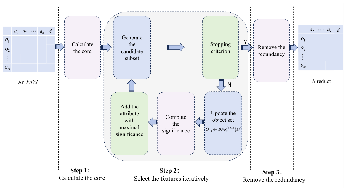
Both Algorithms 3 and 4 mainly contain three parts, as shown in Figure 2. The first part (Lines 2–10) is to calculate the core of an IvDS; the second part (Lines 14–22) is to select the features quickly according to order preservation of the attributes; the third part (Lines 23–29) is to remove redundant attributes from the selected attribute subsets.

Algorithm 4 A fast feature selection algorithm based on conditional entropy, FFSCE

Input: An IvDS $\mathcal{ID}$ and a similarity rate $\beta \in [0,1]$; Output: A reduct $R_{\square }$. 1: $R_{\square }\leftarrow \varnothing$; 2: $Cor{e}_{\square }\leftarrow \varnothing$; 3: Compute ${\mu }_A^{(\beta ,O)}\left(D\right)$; 4: for each $a_s\in A$ do 5:     Compute ${\mu }_{A-\left\{a_s\right\}}^{(\beta ,O)}\left(D\right)$; 6:     $IN{N}_{\square }^{(\beta ,O)}(a_s,A,D)\leftarrow {\mu }_A^{(\beta ,O)}\left(D\right)-{\mu }_{A-\left\{a_s\right\}}^{(\beta ,O)}\left(D\right)$; 7:     if $IN{N}_{\square }^{(\beta ,O)}(a_s,A,D)>0$ then 8:         $Cor{e}_{\square }\leftarrow Cor{e}_{\square }\cup \left\{a_s\right\}$; 9:     end if 10: end for 11: $i\leftarrow 0$; 12: $O_0\leftarrow O$; 13: $R_{\square }\leftarrow Cor{e}_{\square }$; 14: while ${\mu }_{R_{\square }}^{(\beta ,O_i)}\left(D\right)\ne {\mu }_A^{(\beta ,O_i)}\left(D\right)$ do 15:     $O_{i+1}=BN{D}_{R_{\square }}^{(\beta ,O_i)}\left(D\right)$; 16:     for each $a_s\in A-R_{\square }$ do 17:         Compute $OU{T}_{\square }^{(\beta ,O_{i+1})}(a_s,R_{\square },D)$; 18:     end for 19:     $a^{\prime }={argmax}_{a_s\in A-R_{\square }}OU{T}_{\square }^{(\beta ,O_{i+1})}(a_s,R_{\square },D)$; 20:     $R_{\square }\leftarrow R_{\square }\cup \left\{a^{\prime }\right\}$; 21:     $i\leftarrow i+1$; 22: end while 23: $R^{\prime }\leftarrow R_{\square }$; 24: for each $a_s\in R^{\prime }$ do 25:     Compute $IN{N}_{\square }^{(\beta ,O)}(a_s,R_{\square },D)$; 26:     if $IN{N}_{\square }^{(\beta ,O)}(a_s,R_{\square },D)=0$ then 27:         $R_{\square }\leftarrow R_{\square }-\left\{a_s\right\}$; 28:     end if 29: end for 30: return $R_{\square }$.

To compare the complexity of different algorithms, two groups of comparative algorithms are introduced. The first group includes FSDF [35], DF-AR [43] and HRIDF [44], which are dependency function-based algorithms. The second group consists of FSCE [41], CE-AR [43] and HRICE [44], which are Liang’s conditional entropy-based algorithms.

The time complexities of the experimental algorithms are indicated in

Table 3. The time complexities of algorithms based on the dependency function.

Algorithm	Time Complexity
FFSDF	${O\left(\right|O|}^2{\left|A\right|}^2)+O\left({\sum }_{i=1}^{\left|A\right|-|{\mathrm{Core}}_{▵}|}|O_i{|}^2\left(\right|{\mathrm{Core}}_{▵}|+i)\left(\right|A|-|{\mathrm{Core}}_{▵}|-i+1)+O\left({\left|O\right|}^2{\left|R_{▵}\right|}^2\right)\right)$
FSDF [35]	${O\left(\right|O|}^2{\left|A\right|}^2)+O\left({\sum }_{i=1}^{\left|A\right|-|{\mathrm{Core}}_{▵}|}{\left|O\right|}^2\left(\right|{\mathrm{Core}}_{▵}|+i)\left(\right|A|-|{\mathrm{Core}}_{▵}|-i+1)+O\left({\left|O\right|}^2{\left|R_{▵}\right|}^2\right)\right)$
DF-AR [43]	${O\left(\right|O|}^2{\left|A\right|}^2)+O\left({\sum }_{i=1}^{\left|A\right|-|{\mathrm{Core}}_1|}{\left|O\right|}^2\left(\right|{\mathrm{Core}}_1|+i)\left(\right|A|-|{\mathrm{Core}}_1|-i+1)+O\left({\left|O\right|}^2{\left|R_1\right|}^2\right)\right)$
HRIDF [44]	${O\left(\right|O|}^2{\left|A\right|}^2)+O\left({\sum }_{i=1}^{\left|A\right|-|{\mathrm{Core}}_2|}{\left|O\right|}^2\left(\right|{\mathrm{Core}}_2|+i)\left(\right|A|-|{\mathrm{Core}}_2|-i+1)+O\left({\left|O\right|}^2{\left|R_2\right|}^2\right)\right)$

and

Table 4. The time complexities of algorithms based on Liang’s conditional entropy.

Algorithm	Time Complexity
FFSCE	${O\left(\right|O|}^2{\left|A\right|}^2)+O\left({\sum }_{i=1}^{\left|A\right|-|{\mathrm{Core}}_{\square }|}|O_i{|}^2\left(\right|{\mathrm{Core}}_{\square }|+i)\left(\right|A|-|{\mathrm{Core}}_{\square }|-i+1)+O\left({\left|O\right|}^2{\left|R_{\square }\right|}^2\right)\right)$
FSCE [41]	${O\left(\right|O|}^2{\left|A\right|}^2)+O\left({\sum }_{i=1}^{\left|A\right|-|{\mathrm{Core}}_{\square }|}{\left|O\right|}^2\left(\right|{\mathrm{Core}}_{\square }|+i)\left(\right|A|-|{\mathrm{Core}}_{\square }|-i+1)+O\left({\left|O\right|}^2{\left|R_{\square }\right|}^2\right)\right)$
CE-AR [43]	${O\left(\right|O|}^2{\left|A\right|}^2)+O\left({\sum }_{i=1}^{\left|A\right|-|{\mathrm{Core}}_3|}{\left|O\right|}^2\left(\right|{\mathrm{Core}}_3|+i)\left(\right|A|-|{\mathrm{Core}}_3|-i+1)+O\left({\left|O\right|}^2{\left|R_3\right|}^2\right)\right)$
HRICE [44]	${O\left(\right|O|}^2{\left|A\right|}^2)+O\left({\sum }_{i=1}^{\left|A\right|-|{\mathrm{Core}}_4|}{\left|O\right|}^2\left(\right|{\mathrm{Core}}_4|+i)\left(\right|A|-|{\mathrm{Core}}_4|-i+1)+O\left({\left|O\right|}^2{\left|R_4\right|}^2\right)\right)$

. $Cor{e}_1$, $Cor{e}_2$, $Cor{e}_3$ and $Cor{e}_4$ represent the cores of DF-AR, HRIDF, CE-AR and HRICE. $R_1$, $R_2$, $R_3$ and $R_4$ represent the reducts of DF-AR, HRIDF, CE-AR and HRICE. Since $|O_i|=|BN{D}_{R_{\square }}^{(\beta ,O_{i-1})}\left(D\right)|\le |O|$, the computational time of the proposed algorithms FFSDF and FFSCE is generally less than that of other algorithms. Table 3 and Table 4 present the computational complexity of FFSDF and FFSCE.

From Table 3 and Table 4, the worst-case time complexity of the proposed algorithms (FFSDF and FFSCE) is $O\left(\right|O{|}^2\left|A{|}^3\right)$.

The storage of the original interval-valued data matrix requires $O\left(\right|O\left|\right|A\left|\right)$ space. In addition, calculating and storing the pairwise similarity matrix for constructing fuzzy similarity classes need $O\left(\right|O{|}^2)$ space consumption. Thus, the space complexity of the proposed algorithm is $O\left(\right|O\left|\right|A|+|O{|}^2)$. The space complexities of the experimental algorithms are presented in

Table 5. The space complexities of algorithms based on the dependency function.

	FSDF	FFSDF	DF-AR	HRIDF
Space complexity	$O\left(\right|O\left|\right|A|+|O{|}^2)$	$O\left(\right|O\left|\right|A|+|O{|}^2)$	$O\left(\right|O\left|\right|A|+|O{|}^2)$	$O\left(\right|O\left|\right|A|+|O{|}^2)$

and

Table 6. The space complexities of algorithms based on Liang’s conditional entropy.

	FSCE	FFSCE	CE-AR	HRICE
Space complexity	$O\left(\right|O\left|\right|A|+|O{|}^2)$	$O\left(\right|O\left|\right|A|+|O{|}^2)$	$O\left(\right|O\left|\right|A|+|O{|}^2)$	$O\left(\right|O\left|\right|A|+|O{|}^2)$

.

6. Experimental Results and Analyses

In this section, we conduct experiments on fifteen datasets, as shown in

Table 7. Experimental datasets.

No.	Datasets	Abbr.	Types	Objects	Attributes	Classes
1	Lymphography 1	LYM	Nominal	148	18	4
2	Banknote Authentication 1	BAN	Numerical	1372	4	2
3	Car Evaluation 1	CAR	Nominal	1728	6	4
4	Molecular Biology 1	MOL	Nominal	105	57	2
5	Ecoli 1	ECO	Numerical	336	7	8
6	Mammographic Mass 1	MAC	Nominal, Numerical	961	5	2
7	Iris 1	IRI	Numerical	150	4	3
8	Lung Cancer 1	LUN	Numerical	32	56	3
9	Blood Transfusion Service Center 1	TRA	Numerical	748	4	2
10	Wireless Indoor Localization 1	WIF	Numerical	2000	7	4
11	Chess (King-Rook-vs.-King-Pawn) 1	CHE	Nominal	3196	35	2
12	Predict Students’ Dropout and Academic Success 1	DRO	Nominal, Numerical	4424	36	3
13	Liver Patient Dataset 2	LIV	Numerical	583	10	2
14	Fresh Water Fish 3	FWF	Interval	12	13	4
15	Heart Failure Prediction 2	HFP	Interval	918	11	2

¹ https://archive-beta.ics.uci.edu. ² https://www.kaggle.com/datasets. ³ https://github.com/Natandradesa/Kernel-Clustering-for-Interval-Data.

. Datasets 1–12 are UCI datasets, while Datasets 13–15 are real-world datasets. We evaluate the monotonicity of significance measures, feature selection efficiency and results, classification accuracy, robustness, and parameter sensitivity in the experiment. To verify the effectiveness and efficiency of the proposed algorithms, we introduce two groups of comparative feature selection algorithms. The first group includes FFDF [35], DF-AR [43] and HRIDF [44], which are dependency function-based algorithms. The second group consists of FFSCE [41], CE-AR [43] and HRICE [44], which are Liang’s conditional entropy-based algorithms. Algorithms are run on a personal computer with Microsoft Windows 10, Intel(R) Core(TM) i7-10750H CPU @ 2.60 GHz and 16.0 GB memory. The software used in this section is PyCharm 2024.1.1 Professional Edition, and the programming language is Python 3.13.

For Datasets 1–12 (accessed on 17 January 2026) in Table 7, we transform the original UCI datasets into interval-valued datasets. For each original UCI dataset, we take the following steps to generate an interval-valued dataset: (1) If the dataset is incomplete, the missing values can be replaced with the most frequent values within each attribute. (2) The nominal values in a dataset can be replaced with integer values. (3) We use the method introduced by Zhang et al. [45] to generate an interval-valued decision system. $a_s^{sin}\left(o_i\right)$ is the value of the object $o_i\in O$ with respect to the attribute $a_s\in A$ in an original UCI dataset. We extend the single value $a_s^{sin}\left(o_i\right)$ to an interval value $a_s\left(o_i\right)=[l_i^s,u_i^s]$ as follows. The lower bound of $a_s\left(o_i\right)$ can be calculated by $l_i^s=a_s^{sin}\left(o_i\right)-2{\sigma }_s$, and the upper bound of $a_s\left(o_i\right)$ can be calculated by $u_i^s=a_s^{sin}\left(o_i\right)+2{\sigma }_s$, where

$${\sigma }_s=\sqrt{{\displaystyle \frac{1}{\left|O\right|}}\sum _{i=1}^{\left|O\right|}{(a_s^{sin}\left(o_i\right)-{\overline{a}}_s)}^2}$$

(12)

is the standard deviation of attribute values $a_s^{sin}\left(o_i\right)$ and ${\overline{a}}_s={\displaystyle \frac{1}{\left|O\right|}}{\sum }_{i=1}^{\left|O\right|}{a}_s^{sin}\left(o_i\right)$ is the mean of attribute values $a_s^{sin}\left(o_i\right)$, $i=1,2,\dots ,\left|O\right|$. To adapt to the uncertain data environment in real scenarios, single-valued features are extended to interval-valued data. Each original single value is taken as the center point of the interval, and the interval radius is determined by the standard deviation of the corresponding feature. Standard deviation can objectively quantify the dispersion and noise fluctuation of feature distribution, which enables the constructed interval to adaptively reflect the uncertainty of data. This method is widely adopted in rough set and granular computing research.

Dataset 13 (accessed on 20 April 2026) is a real-world liver patient dataset. Considering the characteristics of different attributes and medical knowledge, this dataset is transformed into an interval-valued dataset by adopting the quantile-based equal-frequency discretization method. Dataset 14 (accessed on 22 April 2026) is a real-world interval-valued dataset. Dataset 15 (accessed on 5 May 2026) is a real-world medical interval-valued dataset.

6.1. The Monotonicity of the Significance Measures

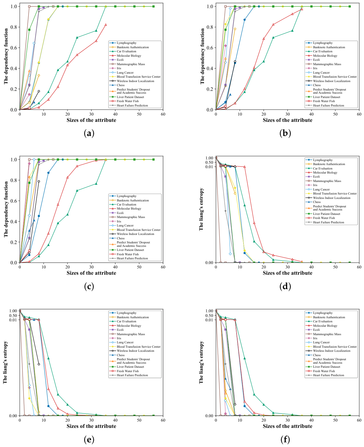
We conduct monotonicity experiments for two measures of attribute significance: the dependency function and Liang’s conditional entropy. In Figure 3, the horizontal axis represents the number of conditional attributes, and the vertical axis denotes the values of the dependency function or Liang’s conditional entropy. Different colors correspond to different experimental datasets. In Figure 3a–c, the dependency function does not decline as the number of attributes grows. In Figure 3d–f, Liang’s conditional entropy presents no increasing tendency with the rising number of attributes.

6.2. Feature Selection Efficiency and Results

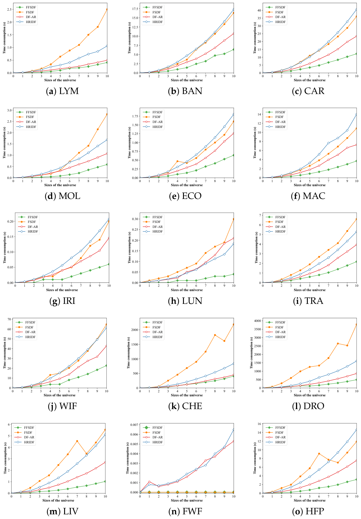
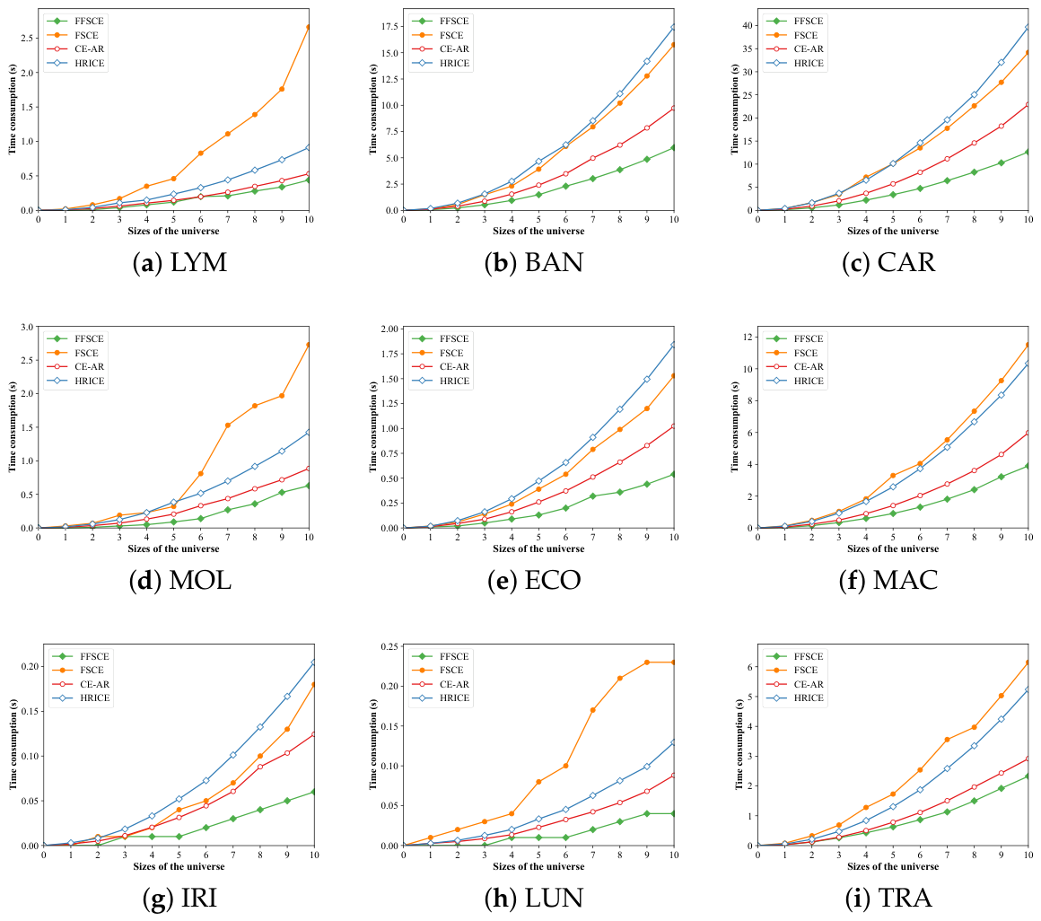
In this subsection, we conduct feature selection experiments on 15 datasets and compare the efficiency of the proposed algorithms (FFSDF and FFSCE) with the other algorithms. Detailed variation trends of FFSDF and the three compared algorithms (FSDF, DF-AR and HRIDF) as the universe increases are illustrated in Figure 4. The horizontal and vertical axes denote the size of the universe (i.e., the size of each sub-dataset) and the execution times of the four algorithms, respectively. The universe of each dataset is divided into 10 equal parts. The first part forms the first sub-dataset, the combination of the first and second parts forms the second sub-dataset, …, and the combination of all ten parts forms the tenth sub-dataset. In the experiments of this subsection, the parameter $\beta$ is set to 0.8.

As indicated in Figure 4, it is apparent that the execution times of the four algorithms generally increase as the sub-dataset size increases. In most datasets, the differences between FFSDF and the other three algorithms in execution time are not distinct in the beginning. The differences between FFSDF and the other three algorithms in execution time become larger when the number of objects increases. For instance, in Figure 4c, the execution time of FFSDF is 10.33 s when the size of the sub-dataset is 9, while those of the other algorithms are 28.73 s, 19.83 s and 32.70 s. The average slopes of the curves of FFSDF are smaller than those of the other three algorithms in general. The execution times of FFSDF increase slightly with the increase in the size of the sub-dataset, while the execution times of the other three algorithms increase greatly. In Figure 4f, the execution time of FFSDF increases by 1.33 s when the size of the sub-dataset varies from 8 to 10, whereas the execution times of the other three algorithms increase by 4.01 s, 2.21 s and 5.25 s; For the same change in the sub-dataset, FFSDF achieves superior performance compared with the other three algorithms.

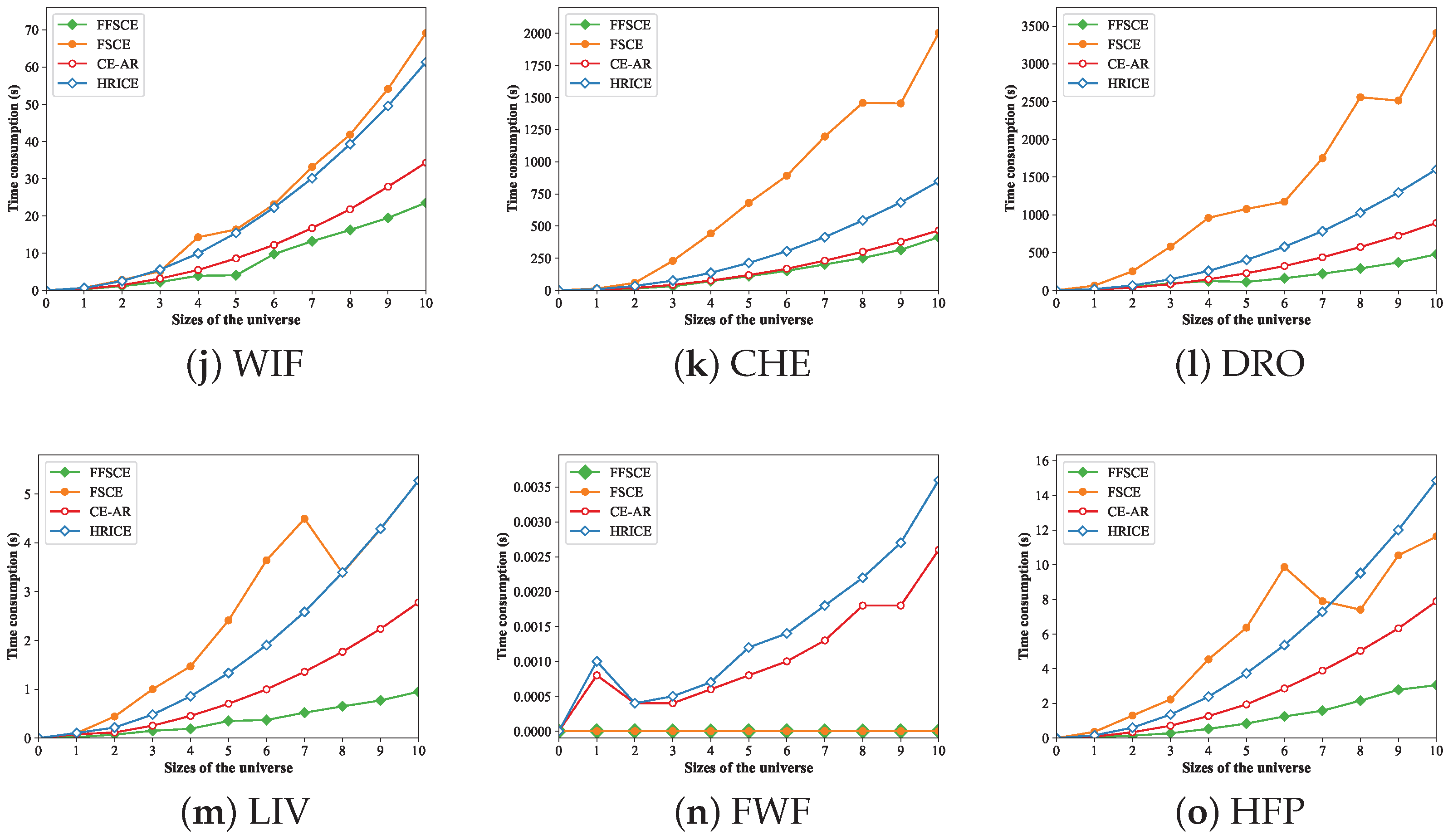
Figure 5 visualizes the change trends of FFSCE and the comparative algorithms with the increase in sub-dataset (the universe). In Figure 5, the X-axis denotes the size of the sub-dataset, while the Y-axis denotes the execution time of the four algorithms. The execution times of the four algorithms increase with the number of objects. In most datasets, the curves of FFSCE rise slowly, while the comparative algorithms rise remarkably when the size of the sub-dataset becomes larger. The relationship between the number of objects and the execution time of FFSCE is not strictly monotonic. For instance, in Figure 5h, the execution times of FFSCE are 0.04 s and 0.04 s when the numbers of objects are 9 and 10. Therefore, the execution time remains unchanged when the size of the dataset varies from 9 to 10.

As shown in

Table 8. Runtime and feature number based on dependency function (s).

No.	Abbr.	FFSDF		FSDF		DF-AR		HRIDF
		Time	Num	Time	Num	Time	Num	Time	Num
1	LYM	0.41	(6)	2.50	(6)	0.50	(17)	1.06	(9)
2	BAN	6.38	(4)	16.34	(4)	10.72	(1)	17.31	(4)
3	CAR	12.23	(6)	36.08	(6)	23.47	(6)	40.59	(6)
4	MOL	0.59	(4)	2.82	(4)	1.08	(12)	1.69	(4)
5	ECO	0.64	(6)	1.60	(6)	1.26	(7)	1.80	(6)
6	MAC	3.70	(5)	10.88	(5)	7.27	(3)	13.99	(5)
7	IRI	0.06	(4)	0.20	(4)	0.15	(4)	0.21	(4)
8	LUN	0.04	(4)	0.30	(4)	0.21	(8)	0.18	(4)
9	TRA	2.18	(3)	6.60	(3)	3.95	(2)	5.29	(3)
10	WIF	22.79	(7)	64.73	(7)	42.82	(2)	61.27	(7)
11	CHE	409.11	(29)	2187.98	(29)	451.95	(31)	839.35	(29)
12	DRO	491.18	(19)	3789.36	(19)	863.41	(36)	1605.67	(30)
13	LIV	1.03	(8)	5.54	(8)	2.70	(8)	5.11	(8)
14	FWF	0.0008	(1)	0.0035	(1)	0.0059	(2)	0.0067	(2)
15	HFP	3.17	(10)	11.89	(10)	7.56	(10)	14.63	(10)
Avg		63.57	(7.73)	409.12	(7.73)	94.47	(9.93)	173.88	(8.73)
Rank		1.00	(2.30)	3.47	(2.30)	2.13	(2.77)	3.40	(2.63)

and

Table 9. Runtime and feature number based on Liang’s conditional entropy (s).

No.	Abbr.	FFSCE		FSCE		CE-AR		HRICE
		Time (s)	Num	Time (s)	Num	Time (s)	Num	Time (s)	Num
1	LYM	0.44	(6)	2.66	(6)	0.53	(17)	0.91	(8)
2	BAN	5.97	(4)	15.77	(4)	9.73	(4)	17.45	(4)
3	CAR	12.65	(6)	34.20	(6)	22.92	(6)	39.69	(6)
4	MOL	0.63	(4)	2.73	(4)	0.89	(12)	1.42	(4)
5	ECO	0.54	(6)	1.53	(6)	1.02	(7)	1.84	(6)
6	MAC	3.90	(5)	11.52	(5)	5.98	(5)	10.35	(5)
7	IRI	0.06	(4)	0.18	(4)	0.12	(4)	0.20	(4)
8	LUN	0.04	(3)	0.23	(3)	0.09	(6)	0.13	(3)
9	TRA	2.33	(3)	6.15	(3)	2.92	(3)	5.24	(3)
10	WIF	23.54	(7)	69.18	(7)	34.33	(7)	61.35	(7)
11	CHE	413.13	(29)	2002.61	(29)	465.94	(31)	848.77	(29)
12	DRO	476.80	(19)	3409.50	(19)	892.87	(36)	1602.47	(30)
13	LIV	0.95	(8)	5.27	(8)	2.78	(8)	5.27	(8)
14	FWF	0.0008	(1)	0.0035	(1)	0.0035	(2)	0.0038	(2)
15	HFP	3.05	(10)	11.63	(10)	7.89	(10)	14.85	(10)
Avg		62.94	(7.67)	371.54	(7.67)	96.53	(10.53)	174.00	(8.60)
Rank		1.00	(2.17)	3.53	(2.17)	2.03	(3.17)	3.43	(2.50)

, Time denotes the feature selection runtime, Num denotes the reduct length (the size of a reduct), Avg represents the average runtime (the number of reducts), Rank indicates the average ranking of runtime (the size of a reduct). The minimum average feature selection time (or feature length) and Rank values are marked in black. For dependency function-based feature selection in Table 8, the average runtime of FFSDF is 63.57 s, while those of FSDF, DF-AR and HRIDF are 409.12 s, 94.47 s and 173.88 s respectively. The feature selection efficiency of FFSDF is significantly higher than that of the other three algorithms. For the dataset DRO, the runtime of FFSDF is 491.18 s, while those of FSDF, DF-AR and HRIDF are 3789.36 s, 863.41 s and 1605.67 s. For the dataset LUN, the runtime of FFSDF is 0.04 s, while those of FSDF, DF-AR and HRIDF are 0.30 s, 0.21 s and 0.18 s. Since FFSDF and FSDF have the same reducts, they have an identical average rank by reduct size. The average rank of FFSDF by reduct size is 2.30, while those of DF-AR and HRIDF are 2.77 and 2.63. Clearly, FFSDF and FSDF have shorter reduct lengths. Detailed feature selection results are presented in

Table 10. Feature selection result comparison (dependency function).

No.	Abbr.	Algorithms	Reduct Length	Reducts
1	LYM	FFSDF(FSDF)	6	$\{2,13,14,15,16,18\}$
		DF-AR	17	$\{1,2,3,4,5,6,7,8,10,11,12,13,14,15,16,17,18\}$
		HRIDF	9	$\{1,2,3,6,10,12,13,14,15\}$
2	BAN	FFSDF(FSDF)	4	$\{1,2,3,4\}$
		DF-AR	1	$\left\{3\right\}$
		HRIDF	4	$\{1,2,3,4\}$
3	CAR	FFSDF(FSDF)	6	$\{1,2,3,4,5,6\}$
		DF-AR	6	$\{1,2,3,4,5,6\}$
		HRIDF	6	$\{1,2,3,4,5,6\}$
4	MOL	FFSDF(FSDF)	4	$\{10,25,40,42\}$
		DF-AR	12	$\{5,17,19,20,24,26,30,34,41,42,45,52\}$
		HRIDF	4	$\{10,25,40,42\}$
5	ECO	FFSDF(FSDF)	6	$\{1,2,3,5,6,7\}$
		DF-AR	7	$\{1,2,3,4,5,6,7\}$
		HRIDF	6	$\{1,2,3,5,6,7\}$
6	MAC	FFSDF(FSDF)	5	$\{1,2,3,4,5\}$
		DF-AR	3	$\{1,2,4\}$
		HRIDF	5	$\{1,2,3,4,5\}$
7	IRI	FFSDF(FSDF)	4	$\{1,2,3,4\}$
		DF-AR	4	$\{1,2,3,4\}$
		HRIDF	4	$\{1,2,3,4\}$
8	LUN	FFSDF(FSDF)	4	$\{1,4,7,42\}$
		DF-AR	8	$\{29,31,40,41,45,46,53,56\}$
		HRIDF	4	$\{1,4,7,42\}$
9	TRA	FFSDF(FSDF)	3	$\{1,2,4\}$
		DF-AR	2	$\{1,2\}$
		HRIDF	3	$\{1,2,4\}$
10	WIF	FFSDF(FSDF)	7	$\{1,2,3,4,5,6,7\}$
		DF-AR	2	$\{1,2\}$
		HRIDF	7	$\{1,2,3,4,5,6,7\}$
11	CHE	FFSDF(FSDF)	29	{1, 3, 4, 5, 6, 7, 9, 10, 12, 13, 15, 16, 17, 18, 20, 21, 23, 24, 25, 26, 27, 28, 30, 31, 32, 33, 34, 35, 36 }
		DF-AR	31	{1, 2, 3, 4, 5, 6, 7, 8, 10, 11, 12, 13, 15, 16, 17, 18, 20, 21, 22, 23, 24, 25, 26, 27, 28, 30, 31, 33, 34, 35, 36}
		HRIDF	29	{1, 3, 4, 5, 6, 7, 9, 10, 11, 12, 13, 15, 16, 17, 18, 20, 21, 23, 24, 25, 26, 27, 28, 30, 31, 33, 34, 35, 36}
12	DRO	FFSDF(FSDF)	19	$\{2,3,7,9,10,12,13,14,16,18,19,20,24,26,27,30,31,34,35\}$
		DF-AR	36	{1, 2, 3, 4, 5, 6, 7, 8, 9, 10, 11, 12, 13, 14, 15, 16, 17, 18, 19, 20, 21, 22, 23, 24, 25, 26, 27, 28, 29, 30, 31, 32, 33, 34, 35, 36}
		HRIDF	30	{1, 2, 3, 4, 5, 6, 7, 9, 10, 12, 13, 14, 15, 16, 17, 18, 19, 20, 21, 22, 24, 25, 27, 29, 30, 31, 32, 33, 34, 35}
13	LIV	FFSDF(FSDF)	8	$\{1,2,3,5,6,7,8,10\}$
		DF-AR	8	$\{1,2,3,5,6,7,8,10\}$
		HRIDF	8	$\{1,2,3,5,6,7,8,10\}$
14	FWF	FFSDF(FSDF)	1	$\left\{3\right\}$
		DF-AR	2	$\{2,3\}$
		HRIDF	2	$\{1,3\}$
15	HFP	FFSDF(FSDF)	10	$\{1,3,4,5,6,7,8,9,10,11\}$
		DF-AR	10	$\{1,3,4,5,6,7,8,9,10,11\}$
		HRIDF	10	$\{1,3,4,5,6,7,8,9,10,11\}$

.

As shown in Table 9, for Liang’s conditional entropy, the average runtime of FFSCE is 62.94 s, while those of FSCE, CE-AR and HRICE are 371.54 s, 96.53 s and 174.00 s respectively. On the same dataset in Table 9, FFSCE consumes the least time compared with the other three algorithms and thus achieves higher efficiency. Since FFSCE and FSCE have the same reducts, they have an identical average rank for reduct size. The average rank of FFSDF for reduct size is 2.17, while those of CE-AR and HRICE are 3.17 and 2.50. Evidently, FFSCE and FSCE have shorter reduct lengths.

Table 11. Feature selection results comparison (Liang’s conditional entropy).

No.	Abbr.	Algorithms	Reduct Length	Reducts
1	LYM	FFSCE(FSCE)	6	$\{2,13,14,15,16,18\}$
		CE-AR	17	$\{1,2,3,4,5,6,7,8,10,11,12,13,14,15,16,17,18\}$
		HRICE	8	$\{1,2,5,6,10,13,14,15\}$
2	BAN	FFSCE(FSCE)	4	$\{1,2,3,4\}$
		CE-AR	4	$\{1,2,3,4\}$
		HRICE	4	$\{1,2,3,4\}$
3	CAR	FFSCE(FSCE)	6	$\{1,2,3,4,5,6\}$
		CE-AR	6	$\{1,2,3,4,5,6\}$
		HRICE	6	$\{1,2,3,4,5,6\}$
4	MOL	FFSCE(FSCE)	4	$\{10,25,40,42\}$
		CE-AR	12	$\{5,17,19,20,24,26,30,34,41,42,45,52\}$
		HRICE	4	$\{10,25,40,42\}$
5	ECO	FFSCE(FSCE)	6	$\{1,2,3,5,6,7\}$
		CE-AR	7	$\{1,2,3,4,5,6,7\}$
		HRICE	6	$\{1,2,3,5,6,7\}$
6	MAC	FFSCE(FSCE)	5	$\{1,2,3,4,5\}$
		CE-AR	5	$\{1,2,3,4,5\}$
		HRICE	5	$\{1,2,3,4,5\}$
7	IRI	FFSCE(FSCE)	4	$\{1,2,3,4\}$
		CE-AR	4	$\{1,2,3,4\}$
		HRICE	4	$\{1,2,3,4\}$
8	LUN	FFSCE(FSCE)	3	$\{3,4,9\}$
		CE-AR	6	$\{2,3,11,26,39,55\}$
		HRICE	3	$\{3,4,9\}$
9	TRA	FFSCE(FSCE)	3	$\{1,2,4\}$
		CE-AR	3	$\{1,2,4\}$
		HRICE	3	$\{1,2,4\}$
10	WIF	FFSCE(FSCE)	7	$\{1,2,3,4,5,6,7\}$
		CE-AR	7	$\{1,2,3,4,5,6,7\}$
		HRICE	7	$\{1,2,3,4,5,6,7\}$
11	CHE	FFSCE(FSCE)	29	{1, 3, 4, 5, 6, 7, 9, 10, 12, 13, 15, 16, 17, 18, 20, 21, 23, 24, 25, 26, 27, 28, 30, 31, 32, 33, 34, 35, 36}
		CE-AR	31	{1, 2, 3, 4, 5, 6, 7, 9, 10, 11, 12, 13, 15, 16, 17, 18, 20, 21, 22, 23, 24, 25, 26, 27, 28, 30, 31, 33, 34, 35, 36}
		HRICE	29	{1, 3, 4, 5, 6, 7, 9, 10, 11, 12, 13, 15, 16, 17, 18, 20, 21, 23, 24, 25, 26, 27, 28, 30, 31, 33, 34, 35, 36}
12	DRO	FFSCE(FSCE)	19	{2, 3, 7, 9, 10, 12, 13, 14, 16, 18, 19, 20, 24, 26, 27, 30, 31, 34, 35}
		CE-AR	36	{1, 2, 3, 4, 5, 6, 7, 8, 9, 10, 11, 12, 13, 14, 15, 16, 17, 18, 19, 20, 21, 22, 23, 24, 25, 26, 27, 28, 29, 30, 31, 32, 33, 34, 35, 36}
		HRICE	30	{1, 2, 3, 4, 5, 6, 7, 9, 10, 12, 13, 14, 15, 16, 17, 18, 19, 20, 21, 22, 24, 25, 27, 29, 30, 31, 32, 33, 34, 35}
13	LIV	FFSCE(FSCE)	8	$\{1,2,3,5,6,7,8,10\}$
		CE-AR	8	$\{1,2,3,5,6,7,8,10\}$
		HRICE	8	$\{1,2,3,5,6,7,8,10\}$
14	FWF	FFSCE(FSCE)	1	$\left\{3\right\}$
		CE-AR	2	$\{2,3\}$
		HRICE	2	$\{1,3\}$
15	HFP	FFSCE(FSCE)	10	$\{1,3,4,5,6,7,8,9,10,11\}$
		CE-AR	10	$\{1,3,4,5,6,7,8,9,10,11\}$
		HRICE	10	$\{1,3,4,5,6,7,8,9,10,11\}$

reports the detailed feature selection results.

6.3. Classification Accuracy Comparison

In this subsection, we compare the classification accuracy of the proposed algorithms with that of other algorithms. The parameter $\beta$ is set to 0.8. We employ SVM and KNN classifiers from the sklearn package with default parameters. The SVM classifier employs $C=1.0$ and the RBF kernel, while the KNN classifier uses a neighbor number of $k=5$.

For the classification accuracy experiment based on the dependency function, the classification accuracies of the reducts obtained by FFSDF are compared with those of FSDF, DF-AR and HRIDF, as shown in

Table 12. Classification accuracy comparison based on dependency function (%).

No.	Abbr.	SVM			KNN
		FFSDF (FSDF)	DF-AR	HRIDF	FFSDF (FSDF)	DF-AR	HRIDF
1	LYM	76.35 ± 2.03	77.03 ± 0.00	72.30 ± 2.03	74.32 ± 0.00	70.95 ± 0.68	71.62 ± 0.00
2	BAN	100.00 ± 0.00	61.44 ± 0.86	100.00 ± 0.00	99.85 ± 0.29	64.43 ± 2.16	99.85 ± 0.29
3	CAR	93.34 ± 2.32	93.34 ± 2.32	93.34 ± 2.32	90.40 ± 7.45	90.40 ± 7.45	90.40 ± 7.45
4	MOL	67.82 ± 12.70	64.55 ± 12.79	67.82 ± 12.70	71.55 ± 13.9	64.09 ± 19.82	64.82 ± 13.37
5	ECO	86.26 ± 1.83	86.26 ± 1.83	86.26 ± 1.83	84.17 ± 2.14	84.17 ± 2.14	84.17 ± 2.14
6	MAC	80.33 ± 3.56	77.84 ± 3.06	80.33 ± 3.56	79.40 ± 4.19	79.30 ± 4.69	79.40 ± 4.19
7	IRI	97.33 ± 3.27	97.33 ± 3.27	97.33 ± 3.27	96.67 ± 4.47	96.67 ± 4.47	96.67 ± 4.47
8	LUN	76.85 ± 12.90	67.59 ± 7.29	76.85 ± 12.90	80.56 ± 14.16	67.59 ± 7.29	80.56 ± 14.16
9	TRA	76.74 ± 1.04	76.07 ± 1.98	76.74 ± 1.04	71.00 ± 10.09	70.34 ± 7.55	71.00 ± 10.09
10	WIF	98.10 ± 1.16	98.10 ± 1.16	98.10 ± 1.16	97.55 ± 1.27	97.55 ± 1.27	97.55 ± 1.27
11	CHE	91.02 ± 9.35	87.57 ± 10.88	87.79 ± 10.83	77.25 ± 4.35	76.59 ± 5.22	75.75 ± 5.14
12	DRO	66.61 ± 0.79	49.93 ± 0.10	49.93 ± 0.10	61.35 ± 1.33	61.10 ± 1.19	60.42 ± 1.69
13	LIV	71.36 ± 0.72	71.36 ± 0.72	71.36 ± 0.72	65.16 ± 6.08	65.16 ± 6.08	65.16 ± 6.08
14	FWF	50.00 ± 0.00	33.33 ± 16.67	50.00 ± 0.00	33.33 ± 16.67	33.33 ± 16.67	33.33 ± 16.67
15	HFP	70.68 ± 8.27	70.68 ± 8.27	70.68 ± 8.27	70.13 ± 7.95	70.13 ± 7.95	70.13 ± 7.95
Avg		80.19 ± 4.00	74.16 ± 4.75	78.59 ± 4.05	76.85 ± 6.29	72.79 ± 6.31	76.06 ± 6.33
Rank		1.67	2.43	1.90	1.60	2.40	2.00

. Avg denotes the average classification accuracy, and Rank represents the average ranking of classification accuracy. The highest classification accuracy and the minimum Rank value are marked in bold. Since FFSDF and FSDF have identical reducts, they achieve the same classification accuracy. Classification accuracy comparisons are conducted on two classifiers, namely, SVM and KNN. As presented in Table 12, for the SVM classifier, the proposed algorithm FFSDF achieves higher classification accuracy than either DF-AR or HRIDF on nine datasets and equal classification accuracy to DF-AR and HRIDF on six datasets. The average classification accuracy of FFSDF is 80.19%, whereas those of DF-AR and HRIDF are 74.16% and 78.59%, respectively. The average classification accuracy of FFSDF is higher than that of DF-AR and HRIDF. The rank value of FFSDF is 1.67, which is lower than the rank values of DF-AR (2.43) and HRIDF (1.90). For the KNN classifier, FFSDF achieves higher classification accuracy than either DF-AR or HRIDF on seven datasets and equal classification accuracy to DF-AR or HRIDF on eight datasets. The average classification accuracy of FFSDF is 76.85%, which is higher than 72.79% (DF-AR) and 76.06% (HRIDF). Meanwhile, the rank value of FFSDF is lower than those of DF-AR and HRIDF.

For the classification accuracy experiment of Liang’s conditional entropy, the classification accuracy of the reducts obtained by FFSCE is compared with those of FSCE, CE-AR and HRICE, as shown in

Table 13. Classification accuracy comparison based on Liang’s conditional entropy (%).

No.	Abbr.	SVM			KNN
		FFSCE (FSCE)	CE-AR	HRICE	FFSCE (FSCE)	CE-AR	HRICE
1	LYM	76.35 ± 2.03	77.03 ± 0.00	74.32 ± 0.00	74.32 ± 0.00	70.95 ± 0.68	72.97 ± 2.70
2	BAN	100.00 ± 0.00	100.00 ± 0.00	100.00 ± 0.00	99.85 ± 0.29	99.85 ± 0.29	99.85 ± 0.29
3	CAR	93.34 ± 2.32	93.34 ± 2.32	93.34 ± 2.32	90.40 ± 7.45	90.40 ± 7.45	90.40 ± 7.45
4	MOL	67.82 ± 12.70	64.55 ± 12.79	67.82 ± 12.70	71.55 ± 13.9	64.09 ± 19.82	64.82 ± 13.37
5	ECO	86.26 ± 1.83	86.26 ± 1.83	86.26 ± 1.83	84.17 ± 2.14	83.87 ± 2.44	83.87 ± 2.44
6	MAC	80.33 ± 3.56	80.33 ± 3.56	76.86 ± 1.52	79.40 ± 4.19	79.09 ± 4.05	71.42 ± 1.55
7	IRI	97.33 ± 3.27	97.33 ± 3.27	97.33 ± 3.27	96.67 ± 4.47	96.67 ± 4.47	96.67 ± 4.47
8	LUN	80.56 ± 14.16	70.37 ± 4.14	80.56 ± 14.16	77.78 ± 23.24	66.67 ± 12.42	77.78 ± 23.24
9	TRA	76.74 ± 1.04	76.74 ± 1.04	76.74 ± 1.04	71.00 ± 10.09	71.00 ± 10.09	71.00 ± 10.09
10	WIF	98.10 ± 1.16	98.10 ± 1.16	98.10 ± 1.16	97.55 ± 1.27	97.55 ± 1.27	97.55 ± 1.27
11	CHE	91.02 ± 9.35	87.63 ± 10.87	87.79 ± 10.83	77.25 ± 4.35	76.72 ± 5.52	75.75 ± 5.14
12	DRO	66.61 ± 0.79	49.93 ± 0.10	49.93 ± 0.10	61.35 ± 1.33	61.10 ± 1.19	60.42 ± 1.69
13	LIV	71.36 ± 0.72	71.36 ± 0.72	71.36 ± 0.72	65.16 ± 6.08	65.16 ± 6.08	65.16 ± 6.08
14	FWF	50.00 ± 0.00	33.33 ± 16.67	50.00 ± 0.00	33.33 ± 16.67	33.33 ± 16.67	33.33 ± 16.67
15	HFP	70.68 ± 8.27	70.68 ± 8.27	70.68 ± 8.27	70.13 ± 7.95	70.13 ± 7.95	70.13 ± 7.95
Avg		80.43 ± 4.08	77.13 ± 4.45	78.74 ± 3.86	76.66 ± 6.89	75.11 ± 6.69	75.41 ± 6.96
Rank		1.73	2.20	2.07	1.57	2.23	2.20

. The highest classification accuracy and the minimum Rank value are marked in bold. Because FFSCE and FSCE yield identical reduct results, they achieve the same classification accuracy. As presented in Table 13, for the SVM classifier, the proposed algorithm FFSCE achieves higher classification accuracy than either CE-AR or HRICE on seven datasets and equal classification accuracy to CE-AR and HRICE on eight datasets. The average classification accuracy of FFSCE is 80.43%, whereas those of CE-AR and HRICE are 77.13% and 78.74%, respectively. The average classification accuracy of FFSCE is higher than that of CE-AR and HRICE. The rank value of FFSCE is 1.73, which is lower than the rank values of CE-AR (2.20) and HRICE (2.07). For the KNN classifier, FFSCE achieves higher classification accuracy than either CE-AR or HRICE on seven datasets and equal classification accuracy to CE-AR or HRICE on eight datasets. The average classification accuracy of FFSCE is 76.66%, which is higher than 75.11% (CE-AR) and 75.41% (HRICE). Meanwhile, the rank value of FFSCE is lower than those of CE-AR and HRICE.

We adopt the Wilcoxon Signed-Rank Test for statistical analysis of the average classification accuracy in Table 12 and Table 13. For dependency-based feature selection in Table 12, compared with the DF-AR algorithm, the p-values of FFSDF (FSDF) on the SVM and KNN classifiers are $0.0117$ and $0.0078$, respectively. It demonstrates that FFSDF achieves a significant advantage in classification accuracy with the SVM and KNN classifiers. In the comparison between FFSDF (FSDF) and HRIDF, the p-values on SVM and KNN are $0.2500$ and $0.1250$. Although the p-values are relatively large, the average classification accuracy of FFSDF on SVM is $80.19\%$, which is higher than the $78.59\%$ of HRIDF in Table 12. The average classification accuracy of FFSDF on KNN is $76.85\%$, exceeding the $76.06\%$ of HRIDF. Therefore, FFSDF is superior in classification accuracy. For Liang’s entropy-based feature selection in Table 13, the p-values of FFSCE (FSCE) versus CE-AR and HRICE on the KNN classifier are $0.0156$ and $0.0313$, which indicates that FFSCE (FSCE) has a remarkable performance advantage for KNN. On the SVM classifier, the corresponding p-values are $0.0625$ and $0.1250$. Although the p-values are relatively large, FFSCE (FSCE) still yields higher classification accuracy than CE-AR and HRICE according to Table 12. The proposed FFSCE yields favorable classification results.

6.4. Robustness Analysis

This subsection mainly conducts robustness tests on the proposed algorithms. Boundary expansion is one of the most common perturbation forms for interval-valued data. The expansion of boundaries directly enlarges the uncertainty range of intervals, and further affects the stability and effectiveness of feature selection algorithms. In this subsection, we test the robustness of the two proposed algorithms (FFSDF and FFSCE) by expanding the upper bounds of interval values. In

Table 14. Comparison of classification accuracy in robustness test using SVM classifier (dependency function) (%).

No.	Abbr.	FFSDF (SVM, 10%)
		Original Datasets	25%	50%	100%	200%
1	LYM	76.35 ± 2.03	75.00 ± 0.68	75.68 ± 2.70	75.68 ± 2.70	75.68 ± 2.70
2	BAN	100.00 ± 0.00	100.00 ± 0.00	100.00 ± 0.00	100.00 ± 0.00	100.00 ± 0.00
3	CAR	93.34 ± 2.32	93.34 ± 2.32	93.34 ± 2.32	93.34 ± 2.32	93.34 ± 2.32
4	MOL	67.82 ± 12.70	54.45 ± 12.79	65.91 ± 14.44	65.82 ± 14.32	50.64 ± 15.05
5	ECO	86.26 ± 1.83	86.26 ± 1.83	86.26 ± 1.83	86.26 ± 1.83	86.26 ± 1.83
6	MAC	80.33 ± 3.56	80.33 ± 3.56	80.33 ± 3.56	80.33 ± 3.56	80.33 ± 3.56
7	IRI	97.33 ± 3.27	97.33 ± 3.27	97.33 ± 3.27	97.33 ± 3.27	97.33 ± 3.27
8	LUN	76.85 ± 12.90	79.63 ± 21.56	66.67 ± 20.03	66.67 ± 20.03	66.67 ± 20.03
9	TRA	76.74 ± 1.04	76.07 ± 0.86	76.07 ± 0.86	76.07 ± 0.86	76.07 ± 0.86
10	WIF	98.10 ± 1.16	98.10 ± 1.16	98.10 ± 1.16	98.10 ± 1.16	98.10 ± 1.16
11	CHE	91.02 ± 9.35	91.17 ± 9.13	89.98 ± 8.27	89.98 ± 8.27	89.98 ± 8.27
12	DRO	66.61 ± 0.79	67.11 ± 0.69	55.36 ± 2.22	55.36 ± 2.22	55.36 ± 2.22
13	LIV	71.36 ± 0.72	71.36 ± 0.72	71.36 ± 0.72	71.36 ± 0.72	71.36 ± 0.72
14	FWF	50.00 ± 0.00	25.00 ± 8.33	25.00 ± 8.33	50.00 ± 0.00	25.00 ± 8.33
15	HFP	70.68 ± 8.27	70.68 ± 8.27	70.78 ± 8.38	70.78 ± 8.38	70.78 ± 8.38
Avg		80.19 ± 4.00	77.72 ± 5.01	76.81 ± 5.21	78.47 ± 4.64	75.79 ± 5.25

,

Table 15. Comparison of classification accuracy in robustness tests using KNN classifier (dependency function) (%).

No.	Abbr.	FFSDF (KNN, 10%)
		Original Datasets	25%	50%	100%	200%
1	LYM	74.32 ± 0.00	73.65 ± 0.68	75.00 ± 0.68	75.00 ± 0.68	75.00 ± 0.68
2	BAN	99.85 ± 0.29	99.85 ± 0.29	99.85 ± 0.29	99.85 ± 0.29	99.85 ± 0.29
3	CAR	90.40 ± 7.45	90.40 ± 7.45	90.40 ± 7.45	90.40 ± 7.45	90.40 ± 7.45
4	MOL	71.55 ± 13.90	50.64 ± 10.48	62.91 ± 13.25	54.36 ± 10.36	50.36 ± 14.72
5	ECO	84.17 ± 2.14	84.17 ± 2.14	84.17 ± 2.14	84.17 ± 2.14	84.17 ± 2.14
6	MAC	79.40 ± 4.19	79.19 ± 4.37	79.19 ± 4.37	79.19 ± 4.37	79.19 ± 4.37
7	IRI	96.67 ± 4.47	96.67 ± 4.47	96.67 ± 4.47	96.67 ± 4.47	96.67 ± 4.47
8	LUN	80.56 ± 14.16	83.33 ± 15.21	80.56 ± 21.15	80.56 ± 21.15	80.56 ± 21.15
9	TRA	71.00 ± 10.09	67.00 ± 13.90	67.00 ± 13.90	67.00 ± 13.90	67.00 ± 13.90
10	WIF	97.55 ± 1.27	97.55 ± 1.27	97.55 ± 1.27	97.55 ± 1.27	97.55 ± 1.27
11	CHE	77.25 ± 4.35	79.07 ± 5.27	82.41 ± 6.31	82.41 ± 6.31	82.41 ± 6.31
12	DRO	61.35 ± 1.33	64.67 ± 1.31	54.66 ± 1.60	54.66 ± 1.60	54.66 ± 1.60
13	LIV	65.16 ± 6.08	67.05 ± 4.22	66.36 ± 4.34	66.36 ± 4.34	66.36 ± 4.34
14	FWF	33.33 ± 16.67	16.67 ± 0.00	16.67 ± 0.00	33.33 ± 16.67	16.67 ± 0.00
15	HFP	70.13 ± 7.95	70.13 ± 7.95	67.42 ± 7.58	67.42 ± 7.58	67.42 ± 7.58
Avg		76.85 ± 6.29	74.67 ± 5.27	74.72 ± 5.92	75.26 ± 6.84	73.88 ± 6.02

,

Table 16. Comparison of classification accuracy in robustness tests using SVM classifier (Liang’s conditional entropy) (%).

No.	Abbr.	FFSCE (SVM, 10%)
		Original Datasets	25%	50%	100%	200%
1	LYM	76.35 ± 2.03	75.00 ± 0.68	75.68 ± 2.70	75.68 ± 2.70	75.68 ± 2.70
2	BAN	100.00 ± 0.00	100.00 ± 0.00	100.00 ± 0.00	100.00 ± 0.00	100.00 ± 0.00
3	CAR	93.34 ± 2.32	93.34 ± 2.32	93.34 ± 2.32	93.34 ± 2.32	93.34 ± 2.32
4	MOL	67.82 ± 12.70	70.18 ± 14.60	63.73 ± 8.61	64.73 ± 15.74	65.55 ± 15.99
5	ECO	86.26 ± 1.83	86.26 ± 1.83	86.26 ± 1.83	86.26 ± 1.83	86.26 ± 1.83
6	MAC	80.33 ± 3.56	80.33 ± 3.56	80.33 ± 3.56	80.33 ± 3.56	80.33 ± 3.56
7	IRI	97.33 ± 3.27	97.33 ± 3.27	97.33 ± 3.27	97.33 ± 3.27	97.33 ± 3.27
8	LUN	80.56 ± 14.16	79.63 ± 21.56	87.04 ± 14.76	87.04 ± 14.76	87.04 ± 14.76
9	TRA	76.74 ± 1.04	76.07 ± 0.86	76.07 ± 0.86	76.07 ± 0.86	76.07 ± 0.86
10	WIF	98.10 ± 1.16	98.10 ± 1.16	98.10 ± 1.16	98.10 ± 1.16	98.10 ± 1.16
11	CHE	91.02 ± 9.35	91.17 ± 9.13	87.85 ± 10.13	87.85 ± 10.13	87.85 ± 10.13
12	DRO	66.61 ± 0.79	67.11 ± 0.69	69.85 ± 1.03	69.82 ± 0.99	69.82 ± 0.99
13	LIV	71.36 ± 0.72	71.36 ± 0.72	71.36 ± 0.72	71.36 ± 0.72	71.36 ± 0.72
14	FWF	50.00 ± 0.00	25.00 ± 8.33	25.00 ± 8.33	50.00 ± 0.00	25.00 ± 8.33
15	HFP	70.68 ± 8.27	70.68 ± 8.27	70.78 ± 8.38	70.78 ± 8.38	70.78 ± 8.38
Avg		80.43 ± 4.08	78.77 ± 5.13	78.85 ± 4.51	80.58 ± 4.43	78.97 ± 5.00

and

Table 17. Comparison of classification accuracy in robustness tests using KNN classifier (Liang’s conditional entropy) (%).

No.	Abbr.	FFSCE (KNN, 10%)
		Original Datasets	25%	50%	100%	200%
1	LYM	74.32 ± 0.00	73.65 ± 0.68	75.00 ± 0.68	75.00 ± 0.68	75.00 ± 0.68
2	BAN	99.85 ± 0.29	99.85 ± 0.29	99.85 ± 0.29	99.85 ± 0.29	99.85 ± 0.29
3	CAR	90.40 ± 7.45	90.40 ± 7.45	90.40 ± 7.45	90.40 ± 7.45	90.40 ± 7.45
4	MOL	71.55 ± 13.90	74.91 ± 15.01	63.64 ± 7.72	66.36 ± 8.78	66.45 ± 19.04
5	ECO	84.17 ± 2.14	84.17 ± 2.14	84.17 ± 2.14	84.17 ± 2.14	84.17 ± 2.14
6	MAC	79.40 ± 4.19	79.19 ± 4.37	79.19 ± 4.37	79.19 ± 4.37	79.19 ± 4.37
7	IRI	96.67 ± 4.47	96.67 ± 4.47	96.67 ± 4.47	96.67 ± 4.47	96.67 ± 4.47
8	LUN	77.78 ± 23.24	83.33 ± 15.21	84.26 ± 14.40	84.26 ± 14.40	84.26 ± 14.40
9	TRA	71.00 ± 10.09	67.00 ± 13.90	67.00 ± 13.90	67.00 ± 13.90	67.00 ± 13.90
10	WIF	97.55 ± 1.27	97.55 ± 1.27	97.55 ± 1.27	97.55 ± 1.27	97.55 ± 1.27
11	CHE	77.25 ± 4.35	79.07 ± 5.27	83.50 ± 5.60	83.50 ± 5.60	83.50 ± 5.60
12	DRO	61.35 ± 1.33	64.67 ± 1.31	60.13 ± 1.34	60.24 ± 1.19	60.24 ± 1.19
13	LIV	65.16 ± 6.08	67.05 ± 4.22	66.36 ± 4.34	66.36 ± 4.34	66.36 ± 4.34
14	FWF	33.33 ± 16.67	16.67 ± 0.00	16.67 ± 0.00	33.33 ± 16.67	16.67 ± 0.00
15	HFP	70.13 ± 7.95	70.13 ± 7.95	67.42 ± 7.58	67.42 ± 7.58	67.42 ± 7.58
Avg		76.66 ± 6.89	76.29 ± 5.57	75.45 ± 5.04	76.75 ± 6.21	75.65 ± 5.78

, we randomly expanded the upper bounds of 10% of all conditional attribute values in each interval-valued dataset. Taking the original interval length as the baseline, the upper bounds were expanded by 25%, 50%, 100% and 200% of the original interval length to investigate the influence of perturbation conditions on the classification accuracy of the proposed algorithms. Avg represents the average classification accuracy, and Rank indicates the average ranking of classification accuracy. $\beta =0.8$ for all experiments in this subsection. The average classification accuracies of the original datasets (datasets without expanded upper bounds of interval values) are marked in bold.

In Table 14, the average classification accuracy of FFSDF on the original datasets (without expansion) is 80.19%, while the average classification accuracies on expanded datasets are 77.72% (25%), 76.81% (50%), 78.47% (100%) and 75.79% (200%) on the SVM classifier. The maximum difference in classification accuracy is 4.40%, and the minimum difference is 1.72%. The classification accuracy changes slightly with the expansion of upper bounds. In Table 15, For the KNN classifier, the average classification accuracy of the proposed algorithm on the original dataset (without expansion) is 76.85%, while the average classification accuracies on expanded datasets are 74.67% (25%), 74.72% (50%), 75.26% (100%) and 73.88% (200%), respectively. After expanding the interval upper bounds to different degrees, the classification accuracies show small differences from the original ones. From Table 14 and Table 15, the proposed algorithm FFSDF demonstrates favorable robustness.

As shown in Table 16, on the SVM classifier, FFSCE achieves an average classification accuracy of 80.43%, while the results of other expanded datasets are 78.77%, 78.85%, 80.58% and 78.97%, respectively. As presented in Table 17, on the KNN classifier, the average classification accuracy of FFSCE is 76.66%, and the corresponding values of expanded datasets are 76.29%, 75.45%, 76.75% and 75.65%. The classification accuracy of FFSCE varies slightly with the expansion of the interval upper bounds. Thus, FFSCE possesses favorable robustness for both SVM and KNN classifiers.

To further verify the robustness of the proposed algorithms, we increase the random selection ratio from 10% to 30%. We randomly select 30% of the conditional attribute values and expand their upper bounds. In

Table 18. Comparison of classification accuracy in robustness tests using SVM classifier (dependency function) (%).

No.	Abbr.	FFSDF (SVM, 30%)
		Original Datasets	25%	50%	100%	200%
1	LYM	76.35 ± 2.03	70.27 ± 2.70	75.68 ± 0.00	75.68 ± 0.00	75.68 ± 0.00
2	BAN	100.00 ± 0.00	100.00 ± 0.00	100.00 ± 0.00	100.00 ± 0.00	100.00 ± 0.00
3	CAR	93.34 ± 2.32	93.34 ± 2.32	93.34 ± 2.32	93.34 ± 2.32	93.34 ± 2.32
4	MOL	67.82 ± 12.70	57.18 ± 12.04	71.27 ± 9.74	54.64 ± 15.10	69.55 ± 14.35
5	ECO	86.26 ± 1.83	86.26 ± 1.83	86.26 ± 1.83	86.26 ± 1.83	86.26 ± 1.83
6	MAC	80.33 ± 3.56	80.33 ± 3.56	80.33 ± 3.56	80.33 ± 3.56	80.33 ± 3.56
7	IRI	97.33 ± 3.27	97.33 ± 3.27	97.33 ± 3.27	97.33 ± 3.27	97.33 ± 3.27
8	LUN	76.85 ± 12.90	87.04 ± 14.76	81.48 ± 17.91	81.48 ± 17.91	81.48 ± 17.91
9	TRA	76.74 ± 1.04	76.07 ± 0.86	76.07 ± 0.86	76.07 ± 0.86	76.07 ± 0.86
10	WIF	98.10 ± 1.16	98.10 ± 1.16	98.10 ± 1.16	98.10 ± 1.16	98.10 ± 1.16
11	CHE	91.02 ± 9.35	86.75 ± 9.49	93.12 ± 5.79	93.12 ± 5.79	93.12 ± 5.79
12	DRO	66.61 ± 0.79	49.93 ± 0.10	61.08 ± 1.09	61.08 ± 1.09	70.66 ± 0.70
13	LIV	71.36 ± 0.72	71.36 ± 0.72	71.36 ± 0.72	71.36 ± 0.72	71.36 ± 0.72
14	FWF	50.00 ± 0.00	25.00 ± 8.33	25.00 ± 8.33	50.00 ± 0.00	25.00 ± 8.33
15	HFP	70.68 ± 8.27	70.57 ± 8.39	70.46 ± 8.14	70.46 ± 8.14	70.46 ± 8.14
Avg		80.19 ± 4.00	76.64 ± 4.64	78.73 ± 4.31	79.28 ± 4.12	79.25 ± 4.60

, the average classification accuracy of FFSDF on the original datasets (without expansion) is 80.19%, while the average classification accuracies on expanded datasets are 76.64 (25%), 78.73 (50%), 79.28 (100%) and 79.25% (200%) on the SVM classifier. The classification accuracy changes slightly with the expansion of the upper bounds. As shown in

Table 19. Comparison of classification accuracy in robustness tests using KNN classifier (dependency function) (%).

No.	Abbr.	FFSDF (KNN, 30%)
		Original Datasets	25%	50%	100%	200%
1	LYM	74.32 ± 0.00	70.95 ± 2.03	74.32 ± 4.05	74.32 ± 4.05	74.32 ± 4.05
2	BAN	99.85 ± 0.29	99.85 ± 0.29	99.85 ± 0.29	99.85 ± 0.29	99.85 ± 0.29
3	CAR	90.40 ± 7.45	90.40 ± 7.45	90.40 ± 7.45	90.40 ± 7.45	90.40 ± 7.45
4	MOL	71.55 ± 13.90	61.91 ± 10.83	66.64 ± 7.67	53.55 ± 11.74	69.36 ± 16.99
5	ECO	84.17 ± 2.14	84.17 ± 2.14	84.17 ± 2.14	84.17 ± 2.14	84.17 ± 2.14
6	MAC	79.40 ± 4.19	79.19 ± 4.37	79.19 ± 4.37	79.19 ± 4.37	79.19 ± 4.37
7	IRI	96.67 ± 4.47	96.67 ± 4.47	96.67 ± 4.47	96.67 ± 4.47	96.67 ± 4.47
8	LUN	80.56 ± 14.16	87.04 ± 14.76	76.85 ± 30.12	76.85 ± 30.12	76.85 ± 30.12
9	TRA	71.00 ± 10.09	67.00 ± 13.90	67.00 ± 13.90	67.00 ± 13.90	67.00 ± 13.90
10	WIF	97.55 ± 1.27	97.55 ± 1.27	97.55 ± 1.27	97.55 ± 1.27	97.55 ± 1.27
11	CHE	77.25 ± 4.35	89.70 ± 4.29	87.98 ± 6.04	87.98 ± 6.04	87.98 ± 6.04
12	DRO	61.35 ± 1.33	56.15 ± 1.48	60.40 ± 1.17	60.40 ± 1.17	67.65 ± 1.29
13	LIV	65.16 ± 6.08	65.33 ± 6.31	67.57 ± 5.47	67.57 ± 5.47	67.57 ± 5.47
14	FWF	33.33 ± 16.67	16.67 ± 0.00	16.67 ± 0.00	33.33 ± 16.67	16.67 ± 0.00
15	HFP	70.13 ± 7.95	70.13 ± 7.95	70.03 ± 8.09	70.03 ± 8.09	70.03 ± 8.09
Avg		76.85 ± 6.29	75.51 ± 5.44	75.69 ± 6.43	75.92 ± 7.82	76.35 ± 7.06

, for the KNN classifier, the average classification accuracy of the proposed algorithm on the original dataset (without expansion) is 76.85%, while the average classification accuracies on expanded datasets are 75.51% (25%), 75.69% (50%), 75.92% (100%) and 76.35% (200%). The classification accuracy shows no significant variation when the upper bounds of interval values are expanded with different proportions. When we randomly expand the upper bounds of 30% of all conditional attribute values in each interval-valued dataset, the proposed algorithm FFSDF demonstrates favorable robustness. From Table 18 and Table 19, the average classification accuracies of the original datasets (datasets without expanded upper bounds of interval values) are marked in bold.

In

Table 20. Comparison of classification accuracy in robustness tests using SVM classifier (Liang’s conditional entropy) (%).

No.	Abbr.	FFSCE (SVM, 30%)
		Original Datasets	25%	50%	100%	200%
1	LYM	76.35 ± 2.03	70.27 ± 2.70	75.00 ± 0.68	75.00 ± 0.68	75.68 ± 0.00
2	BAN	100.00 ± 0.00	100.00 ± 0.00	100.00 ± 0.00	100.00 ± 0.00	100.00 ± 0.00
3	CAR	93.34 ± 2.32	93.34 ± 2.32	93.34 ± 2.32	93.34 ± 2.32	93.34 ± 2.32
4	MOL	67.82 ± 12.70	65.36 ± 15.23	73.64 ± 11.11	60.82 ± 11.20	66.64 ± 9.40
5	ECO	86.26 ± 1.83	86.26 ± 1.83	86.26 ± 1.83	86.26 ± 1.83	86.26 ± 1.83
6	MAC	80.33 ± 3.56	80.33 ± 3.56	80.33 ± 3.56	80.33 ± 3.56	80.33 ± 3.56
7	IRI	97.33 ± 3.27	97.33 ± 3.27	97.33 ± 3.27	97.33 ± 3.27	97.33 ± 3.27
8	LUN	80.56 ± 14.16	87.04 ± 14.76	80.56 ± 21.15	80.56 ± 21.15	70.37 ± 4.14
9	TRA	76.74 ± 1.04	76.07 ± 0.86	76.07 ± 0.86	76.07 ± 0.86	76.07 ± 0.86
10	WIF	98.10 ± 1.16	98.10 ± 1.16	98.10 ± 1.16	98.10 ± 1.16	98.10 ± 1.16
11	CHE	91.02 ± 9.35	86.79 ± 9.69	85.78 ± 9.90	85.78 ± 9.90	85.78 ± 9.90
12	DRO	66.61 ± 0.79	65.28 ± 1.26	70.91 ± 0.90	68.54 ± 1.82	70.00 ± 0.99
13	LIV	71.36 ± 0.72	71.36 ± 0.72	71.36 ± 0.72	71.36 ± 0.72	71.36 ± 0.72
14	FWF	50.00 ± 0.00	25.00 ± 8.33	25.00 ± 8.33	50.00 ± 0.00	25.00 ± 8.33
15	HFP	70.68 ± 8.27	70.57 ± 8.39	70.46 ± 8.14	70.46 ± 8.14	70.46 ± 8.14
Avg		80.43 ± 4.08	78.21 ± 4.94	78.94 ± 4.93	79.60 ± 4.44	77.78 ± 3.64

, the average classification accuracy of FFSCE on the original datasets (without expansion) is 80.43%, while the average classification accuracies on expanded datasets are 78.21 (25%), 78.94 (50%), 79.60 (100%) and 77.78 (200%) on the SVM classifier. The classification accuracy changes slightly with the expansion of upper bounds. As shown in

Table 21. Comparison of classification in robustness tests using KNN classifier (Liang’s conditional entropy) (%).

No.	Abbr.	FFSCE (KNN, 30%)
		Original Datasets	25%	50%	100%	200%
1	LYM	74.32 ± 0.00	70.95 ± 2.03	70.95 ± 3.38	70.95 ± 3.38	74.32 ± 4.05
2	BAN	99.85 ± 0.29	99.85 ± 0.29	99.85 ± 0.29	99.85 ± 0.29	99.85 ± 0.29
3	CAR	90.40 ± 7.45	90.40 ± 7.45	90.40 ± 7.45	90.40 ± 7.45	90.40 ± 7.45
4	MOL	71.55 ± 13.90	64.36 ± 16.58	71.55 ± 11.58	58.00 ± 14.11	69.64 ± 12.23
5	ECO	84.17 ± 2.14	84.17 ± 2.14	84.17 ± 2.14	84.17 ± 2.14	84.17 ± 2.14
6	MAC	79.40 ± 4.19	79.19 ± 4.37	79.19 ± 4.37	79.19 ± 4.37	79.19 ± 4.37
7	IRI	96.67 ± 4.47	96.67 ± 4.47	96.67 ± 4.47	96.67 ± 4.47	96.67 ± 4.47
8	LUN	77.78 ± 23.24	87.04 ± 14.76	80.56 ± 21.15	80.56 ± 21.15	69.44 ± 16.20
9	TRA	71.00 ± 10.09	67.00 ± 13.90	67.00 ± 13.90	67.00 ± 13.90	67.00 ± 13.90
10	WIF	97.55 ± 1.27	97.55 ± 1.27	97.55 ± 1.27	97.55 ± 1.27	97.55 ± 1.27
11	CHE	77.25 ± 4.35	84.42 ± 7.66	82.48 ± 3.06	82.48 ± 3.06	82.48 ± 3.06
12	DRO	61.35 ± 1.33	59.74 ± 1.58	62.70 ± 1.22	62.27 ± 1.52	60.90 ± 2.01
13	LIV	65.16 ± 6.08	65.33 ± 6.31	66.36 ± 4.34	66.36 ± 4.34	66.36 ± 4.34
14	FWF	33.33 ± 16.67	16.67 ± 0.00	16.67 ± 0.00	33.33 ± 16.67	16.67 ± 0.00
15	HFP	70.13 ± 7.95	70.13 ± 7.95	70.03 ± 8.09	70.03 ± 8.09	70.03 ± 8.09
Avg		76.66 ± 6.89	75.56 ± 6.05	75.74 ± 5.78	75.92 ± 7.08	74.98 ± 5.59

, for the KNN classifier, the average classification accuracy of the proposed algorithm on the original dataset (without expansion) is 76.66%, while the average classification accuracies on expanded datasets are 75.56% (25%), 75.74% (50%), 75.92% (100%) and 74.98% (200%), respectively. After expanding the interval upper bounds to different degrees, the classification accuracies show small differences from the original ones. From Table 20 and Table 21, the average classification accuracies of the original datasets (datasets without expanded upper bounds of interval values) are marked in bold. The proposed algorithm FFSCE demonstrates robustness.

From Table 14, Table 15, Table 16, Table 17, Table 18, Table 19, Table 20 and Table 21, the classification accuracy of the proposed FFSDF and FFSCE algorithms changes slightly with the expansion of the upper bound of interval values and the increase in the random proportion of selected expanded data. Therefore, FFSDF and FFSCE possess favorable robustness.

6.5. $\beta$-Sensitivity Analysis

In this subsection, we test the sensitivity of the proposed algorithms to the parameter $\beta$. The parameter $\beta$ is set to 0.6, 0.7, and 0.8.

Table 22. Comparison of classification accuracy for different similarity degrees based on FFSDF (%).

No.	Abbr.	SVM			KNN
		0.6	0.7	0.8	0.6	0.7	0.8
1	LYM	72.30 ± 2.03	72.97 ± 1.35	76.35 ± 2.03	75.68 ± 1.35	73.65 ± 0.68	74.32 ± 0.00
2	BAN	100.00 ± 0.00	100.00 ± 0.00	100.00 ± 0.00	99.85 ± 0.29	99.85 ± 0.29	99.85 ± 0.29
3	CAR	93.34 ± 2.32	93.34 ± 2.32	93.34 ± 2.32	90.40 ± 7.45	90.40 ± 7.45	90.40 ± 7.45
4	MOL	63.91 ± 13.50	68.82 ± 12.04	67.82 ± 12.70	66.64 ± 15.85	72.82 ± 17.07	71.55 ± 13.90
5	ECO	86.26 ± 1.83	86.26 ± 1.83	86.26 ± 1.83	84.17 ± 2.14	84.17 ± 2.14	84.17 ± 2.14
6	MAC	80.33 ± 3.56	80.33 ± 3.56	80.33 ± 3.56	79.19 ± 4.37	79.19 ± 4.37	79.40 ± 4.19
7	IRI	97.33 ± 3.27	97.33 ± 3.27	97.33 ± 3.27	96.67 ± 4.47	96.67 ± 4.47	96.67 ± 4.47
8	LUN	76.85 ± 12.90	76.85 ± 12.90	76.85 ± 12.90	80.56 ± 14.16	80.56 ± 14.16	80.56 ± 14.16
9	TRA	76.74 ± 1.04	76.74 ± 1.04	76.74 ± 1.04	71.00 ± 10.09	71.00 ± 10.09	71.00 ± 10.09
10	WIF	98.10 ± 1.16	98.10 ± 1.16	98.10 ± 1.16	97.55 ± 1.27	97.55 ± 1.27	97.55 ± 1.27
11	CHE	91.02 ± 9.35	91.02 ± 9.35	91.02 ± 9.35	77.25 ± 4.35	77.25 ± 4.35	77.25 ± 4.35
12	DRO	68.20 ± 1.05	66.00 ± 0.74	66.61 ± 0.79	62.00 ± 2.05	63.63 ± 1.22	61.35 ± 1.33
13	LIV	71.36 ± 0.72	71.36 ± 0.72	71.36 ± 0.72	65.16 ± 6.08	65.16 ± 6.08	65.16 ± 6.08
14	FWF	8.33 ± 8.33	50.00 ± 0.00	50.00 ± 0.00	16.67 ± 0.00	33.33 ± 16.67	33.33 ± 16.67
15	HFP	70.68 ± 8.27	70.68 ± 8.27	70.68 ± 8.27	70.13 ± 7.95	70.13 ± 7.95	70.13 ± 7.95
Avg		76.98 ± 4.62	79.99 ± 3.90	80.19 ± 4.00	75.53 ± 5.46	77.02 ± 6.55	76.85 ± 6.29

and

Table 23. Comparison of classification accuracy for different similarity degrees based on FFSCE (%).

No.	Abbr.	SVM			KNN
		0.6	0.7	0.8	0.6	0.7	0.8
1	LYM	74.32 ± 0.00	72.97 ± 1.35	76.35 ± 2.03	72.97 ± 2.70	77.70 ± 6.08	74.32 ± 0.00
2	BAN	100.00 ± 0.00	100.00 ± 0.00	100.00 ± 0.00	99.85 ± 0.29	99.85 ± 0.29	99.85 ± 0.29
3	CAR	93.34 ± 2.32	93.34 ± 2.32	93.34 ± 2.32	90.40 ± 7.45	90.40 ± 7.45	90.40 ± 7.45
4	MOL	67.82 ± 12.70	70.27 ± 13.53	67.82 ± 12.70	69.64 ± 13.87	73.36 ± 16.56	71.55 ± 13.90
5	ECO	86.26 ± 1.83	86.26 ± 1.83	86.26 ± 1.83	84.17 ± 2.14	84.17 ± 2.14	84.17 ± 2.14
6	MAC	80.33 ± 3.56	80.33 ± 3.56	80.33 ± 3.56	79.19 ± 4.37	79.19 ± 4.37	79.40 ± 4.19
7	IRI	97.33 ± 3.27	97.33 ± 3.27	97.33 ± 3.27	96.67 ± 4.47	96.67 ± 4.47	96.67 ± 4.47
8	LUN	80.56 ± 14.16	80.56 ± 14.16	80.56 ± 14.16	77.78 ± 23.24	77.78 ± 23.24	77.78 ± 23.24
9	TRA	76.74 ± 1.04	76.74 ± 1.04	76.74 ± 1.04	71.00 ± 10.09	71.00 ± 10.09	71.00 ± 10.09
10	WIF	98.10 ± 1.16	98.10 ± 1.16	98.10 ± 1.16	97.55 ± 1.27	97.55 ± 1.27	97.55 ± 1.27
11	CHE	91.02 ± 9.35	91.02 ± 9.35	91.02 ± 9.35	77.25 ± 4.35	77.25 ± 4.35	77.25 ± 4.35
12	DRO	68.20 ± 1.05	66.79 ± 0.62	66.61 ± 0.79	62.00 ± 2.05	63.36 ± 1.10	61.35 ± 1.33
13	LIV	71.36 ± 0.72	71.36 ± 0.72	71.36 ± 0.72	65.16 ± 6.08	65.16 ± 6.08	65.16 ± 6.08
14	FWF	8.33 ± 8.33	50.00 ± 0.00	50.00 ± 0.00	16.67 ± 0.00	33.33 ± 16.67	33.33 ± 16.67
15	HFP	70.68 ± 8.27	70.68 ± 8.27	70.68 ± 8.27	70.13 ± 7.95	70.13 ± 7.95	70.13 ± 7.95
Avg		77.63 ± 4.52	80.38 ± 4.08	80.43 ± 4.08	75.36 ± 6.02	77.13 ± 7.47	76.66 ± 6.89

present the classification accuracy of the FFSDF and FFSCE algorithms under different parameter values. Across different parameter settings, the classification accuracy of the algorithms remains stable, which means the algorithms possess superior stability and robustness.

In the interval-valued decision system based on the tolerance relation, the similarity threshold $\beta \in [0,1]$ controls the granularity of the tolerance or similarity class. In practical applications, an appropriate value of $\beta$ is selected according to practical needs. According to existing research on interval-valued decision systems, the threshold is commonly set within the range $\beta \in [0.5,0.8]$. As $\beta$ increases, the tolerance classes become finer, and the certainty of the system rises, while the generalization ability decreases; as $\beta$ decreases, the tolerance classes become coarser, and the anti-noise capability is enhanced, yet the discrimination ability declines. The selection mechanism of the threshold $\beta$ will be further investigated in our future work.

7. Conclusions

The key innovations and contributions are listed as follows: (1) We establish a hierarchical approximation model and study the relative theorems. (2) We propose the order preservation of attribute significance in an IvDS. (3) By using the order-preservation strategy of condition attribute importance, and we develop two efficient algorithms based on the dependency function and Liang’s conditional entropy. By selecting attributes on a dwindling universe, the proposed algorithms achieve higher efficiency and obtain the same reduction results as classical dependency degree-based and Liang’s conditional entropy-based algorithms.

Limitations of this work are summarized as follows: (1) Experiments in this paper are carried out on twelve UCI datasets and three real-world datasets. Sufficient tests on large-scale real-world interval-valued datasets are not conducted. The extreme expansion of the upper and lower bounds of interval values is not considered. (2) The Jaccard similarity measure for interval data exhibits sensitivity to outliers in upper and lower bounds, which needs further optimization. (3) The hierarchical granular structure constructed by interval-valued information has not been deeply explored from the perspective of lattice and order-theoretic properties.

In the future, we will focus on addressing the existing limitations of this work, and the specific research directions are as follows: (1) We will conduct extensive experimental verification on a large number of real-world interval-valued datasets. Feature selection in the case of extreme expansion of interval upper and lower bounds should be further studied. (2) We will introduce more robust interval distance measures that are insensitive to boundary noise to improve the anti-noise performance of the model. (3) We will conduct in-depth research on the hierarchical granular structure generated by interval-valued data from the perspective of lattice and order-theoretic properties and explore the inherent relationship between interval-valued information and hierarchical granular computing. (4) We will further explore the effect of the $\beta$ value on feature selection and the computation of the optimal $\beta$ value.

References

1. Song, X.F.; Ma, H.; Zhang, Y.; Gong, D.W.; Guo, Y.N.; Hu, Y. A streaming feature selection method based on dynamic feature clustering and particle swarm optimization. IEEE Trans. Evol. Comput. 2025, 29, 1888–1902. [Google Scholar] [CrossRef]
2. Wang, C.C.; Pechenizkiy, M.; Wei, J.M.; Liu, J. Feature selection via dynamic feature graph. IEEE Trans. Knowl. Data Eng. 2026, 38, 1754–1767. [Google Scholar] [CrossRef]
3. Dai, J.H.; Wang, J. Online multilabel streaming feature selection with missing features by dual-space consistency information measurement. IEEE Trans. Artif. Intell. 2026, 7, 610–624. [Google Scholar] [CrossRef]
4. Hou, C.Z.; Yuan, Z.J.; Zhang, Y.; Lei, Z.Y.; Gao, S.C. Temporal difference reinforcement learning-based ant colony optimization with extremized probability construction for feature selection. Results Eng. 2026, 25, 109721. [Google Scholar] [CrossRef]
5. El-Bably, M.K.; Hosny, R.A.; El-Gayar, M.A. Innovative rough set approaches using novel initial-neighborhood systems: Applications in medical diagnosis of COVID-19 variants. Inf. Sci. 2025, 708, 122044. [Google Scholar] [CrossRef]
6. Abu-Gdairi, R.; El-Bably, M.K. The accurate diagnosis for COVID-19 variants using nearly initial-rough sets. Heliyon 2024, 10, E31288. [Google Scholar] [CrossRef]
7. Bhattacharya, A.; Etemi, B.P.; Samanta, D. Rough set based feature selection model for diabetic retinopathy classification. Frankl. Open 2026, 14, 100491. [Google Scholar] [CrossRef]
8. El-Bably, M.K.; Abu-Gadiri, R.; Fleifel, K.K.; El-Gayar, M.A. Three methods to generalize Pawlak approximations via simply open concepts with economic applications. Soft Comput. 2022, 26, 4685–4700. [Google Scholar] [CrossRef]
9. El-Gayar, M.A.; Abu-Gdairi, R.; El-Bably, M.K.; Taher, D.I. Economic decision-making using rough topological structures. J. Math. 2023, 1, 723233. [Google Scholar] [CrossRef]
10. Pawlak, Z. Rough sets. Int. J. Comput. Inf. Sci. 1982, 11, 341–346. [Google Scholar] [CrossRef]
11. Sang, B.B.; Yang, L.; Chen, H.M.; Li, T.R.; Xu, W.H. Robust attribute reduction exploring class-separability and attribute-correlation for ordered decision systems. IEEE Trans. Syst. Man Cybern. Syst. 2025, 55, 3941–3953. [Google Scholar] [CrossRef]
12. Dai, J.H.; Zhu, Z.L.; Zou, X.T. Fuzzy rough attribute reduction based on fuzzy implication granularity information. IEEE Trans. Fuzzy Syst. 2024, 32, 3741–3752. [Google Scholar] [CrossRef]
13. Ding, W.P.; Sun, Y.; Ling, M.; Liu, J.; Ju, H.R.; Huang, J.S. A novel spark-based attribute reduction and neighborhood classification for rough evidence. IEEE Trans. Cybern. 2024, 54, 1470–1483. [Google Scholar] [CrossRef] [PubMed]
14. Gao, Y.; Chen, D.G.; Wang, H.; Shi, R.F. Optimization attribute reduction with fuzzy rough sets based on algorithm stability. IEEE Trans. Fuzzy Syst. 2024, 32, 2052–2062. [Google Scholar] [CrossRef]
15. Ma, Z.M.; Mi, J.S.; Lin, G.P.; Wu, W.Z. A comparative study of boundary-based rough set models and their feature selection mechanisms. Appl. Soft Comput. 2026, 188, 114317. [Google Scholar] [CrossRef]
16. Zou, X.T.; Dai, J.H. Fuzzy rough feature selection via stripped decision β-neighborhood set and misclassification ratio. Fuzzy Sets Syst. 2025, 520, 109544. [Google Scholar] [CrossRef]
17. Ju, H.R.; Yin, T.; Huang, J.S.; Ding, W.P.; Yang, X.B. Sparse mutual granularity-based feature selection and its application of schizophrenia patients. IEEE Trans. Emerg. Top. Comput. Intell. 2024, 8, 604–614. [Google Scholar] [CrossRef]
18. Xu, R.Y.; Wu, D.; Wang, R.F.; Luo, X. A highly-accurate three-Way decision-incorporated online sparse streaming features selection model. IEEE Trans. Syst. Man Cybern. Syst. 2025, 55, 4258–4272. [Google Scholar] [CrossRef]
19. Zhang, N.; Gao, X.Y.; Yu, T.Y. Heuristic approaches to attribute reduction for generalized decision preservation. Appl. Sci. 2019, 9, 2841. [Google Scholar] [CrossRef]
20. Qian, Y.H.; Liang, J.Y.; Pedrycz, W.; Dang, C.Y. Positive approximation: An accelarator for attribute reduction in rough set thoery. Artif. Intell. 2010, 174, 595–618. [Google Scholar] [CrossRef]
21. Qian, W.B.; Shu, W.H. Mutual information criterion for feature selection from incomplete data. Neurocomputing 2015, 168, 210–220. [Google Scholar] [CrossRef]
22. Leung, Y.; Fischer, M.M.; Wu, W.Z.; Mi, J.S. A rough set approach for the discovery of classification rules in interval-valued information systems. Int. J. Approx. Reason. 2008, 47, 233–246. [Google Scholar] [CrossRef]
23. Qian, Y.H.; Liang, J.Y.; Dang, C.Y. Interval ordered information systems. Comput. Math. Appl. 2008, 56, 1994–2009. [Google Scholar] [CrossRef]
24. Yang, X.B.; Qi, Y.; Yu, D.J.; Yu, H.L.; Yang, J.Y. α-Dominance relation and rough sets in interval-valued information systems. Inf. Sci. 2015, 294, 334–347. [Google Scholar] [CrossRef]
25. Miao, D.Q.; Zhang, N.; Yue, X.D. Knowledge reduction in interval-valued information systems. In Proceedings of the 8th IEEE International Conference on Cognitive Informatics, Hong Kong, China, 15–17 June 2009; pp. 320–327. [Google Scholar] [CrossRef]
26. Du, W.S.; Hu, B.Q. Approximate distribution reducts in inconsistent interval-valued ordered decision tables. Inf. Sci. 2014, 271, 93–114. [Google Scholar] [CrossRef]
27. Li, W.T.; Deng, C.J.; Pedrycz, W.; Ding, W.P.; Hu, X.C.; Zhang, C.; Zhan, T. Dominance-based feature selection approach to interval-valued ordered intuitionistic fuzzy data. Appl. Soft Comput. 2026, 186, 114228. [Google Scholar] [CrossRef]
28. Wang, L.; Liu, Y.Y.; Qin, K.Y.; Pei, Z. Matrix-driven feature selection for interval-valued data based on double fuzzy adaptive neighborhood consistency measure. Fuzzy Sets Syst. 2026, 532, 109795. [Google Scholar] [CrossRef]
29. Qin, Y.J.; Lin, G.P.; Lin, Y.D.; Kou, Y.; Hu, W.Y. Dominance relation-based feature selection for interval-valued multi-label ordered information system. Expert Syst. Appl. 2025, 274, 126898. [Google Scholar] [CrossRef]
30. Xu, W.H.; Tian, Z.Y. Feature selection and information fusion based on preference ranking organization method in interval-valued multi-source decision-making information systems. Inf. Sci. 2025, 700, 121860. [Google Scholar] [CrossRef]
31. Chen, B.W.; Zhang, X.Y.; Yang, J.L. Feature selections based on three improved condition entropies and one new similarity degree in interval-valued decision systems. Eng. Appl. Artif. Intell. 2023, 126, 107165. [Google Scholar] [CrossRef]
32. Yao, Y.Y.; Zhao, Y. Attribute reduction in decision-theoretic rough set models. Inf. Sci. 2008, 178, 3356–3373. [Google Scholar] [CrossRef]
33. Zhang, X.Y.; Li, J.R. Incremental feature selection approach to interval-valued fuzzy decision information systems based on λ-fuzzy similarity self-information. Inf. Sci. 2023, 625, 593–619. [Google Scholar] [CrossRef]
34. Dai, J.H.; Hu, H.; Zheng, G.J.; Hu, Q.H.; Han, H.F.; Shi, H. Attribute reduction in interval-valued information systems based on information entropies. Front. Inf. Technol. Electron. Eng. 2016, 17, 919–928. [Google Scholar] [CrossRef]
35. Xu, F.F.; Lei, J.S.; Bi, Z.Q.; Miao, D.Q.; Du, H.Z. Approaches to approximate reduction with interval-valued multi-decision tables in big data. Chin. J. Softw. 2014, 25, 2119–2135. [Google Scholar] [CrossRef]
36. Zhang, J.; Zhang, X.Y.; Xu, W.H. Attribute reduction in interval-valued fuzzy ordered decision tables via evidence theory. J. Eng. 2018, 2018, 1475–1482. [Google Scholar] [CrossRef]
37. Dai, J.H.; Wang, W.T.; Xu, Q.; Tian, H.W. Uncertainty measurement for interval-valued decision systems based on extended conditional entropy. Knowl.-Based Syst. 2012, 27, 443–450. [Google Scholar] [CrossRef]
38. Xie, N.X.; Liu, M.; Li, Z.W.; Zhang, G.Q. New measures of uncertainty for an interval-valued information system. Inf. Sci. 2019, 470, 156–174. [Google Scholar] [CrossRef]
39. Levandowsky, M.; Winter, D. Distance between sets. Nature 1971, 234, 34–35. [Google Scholar] [CrossRef]
40. Conci, A.; Kubrusly, C. Distances between sets—A survey. Adv. Math. Sci. Appl. 2017, 26, 1–18. [Google Scholar] [CrossRef]
41. Liang, J.Y.; Shi, Z.Z.; Li, D.Y. Information entropy, rough entropy and knowledge granulation in incomplete information systems. Int. J. Gen. Syst. 2006, 35, 641–654. [Google Scholar] [CrossRef]
42. Zhang, X.; Mei, C.L.; Chen, D.G.; Li, J.H. Feature selection in mixed data: A method using a novel fuzzy rough set-based information entropy. Pattern Recognit. 2016, 56, 1–5. [Google Scholar] [CrossRef]
43. Liu, X.; Chen, B.W.; Chen, D.G.; Li, J.H. Attribute reductions based on δ-fusion condition entropy and harmonic similarity degree in interval-valued decision systems. J. Intell. Fuzzy Syst. 2023, 46, 1–14. [Google Scholar] [CrossRef]
44. Tang, P.F.; Mo, Z.W.; Xie, X. Attribute Reduction Based on Relative Knowledge Granularity in Interval-valued Decision Table. J. Chongqing Univ. Technol. (Nat. Sci.) 2021, 35, 286–292. [Google Scholar] [CrossRef]
45. Zhang, X.; Mei, C.L.; Chen, D.G.; Li, J.H. Multi-confidence rule acquisition and confidence-preserved attribute reduction in interval-valued decision systems. Int. J. Approx. Reason. 2014, 55, 1787–1804. [Google Scholar] [CrossRef]
Figure 1. The similarity between two interval values.
Symmetry 18 00849 g001
Figure 2. The process of fast feature selection.
Symmetry 18 00849 g002
Figure 3. (a) Monotonicity of the dependency function ( β = 0.6 ). (b) Monotonicity of the dependency function ( β = 0.7 ). (c) Monotonicity of the dependency function ( β = 0.8 ). (d) Monotonicity of Liang’s conditional entropy ( β = 0.6 ). (e) Monotonicity of Liang’s conditionalentropy ( β = 0.7 ). (f) Monotonicity of Liang’s conditional entropy ( β = 0.8 ).
Symmetry 18 00849 g003
Figure 4. Runtime of FFSDF and other algorithms versus attribute size ( β = 0.8 ).
Symmetry 18 00849 g004
Figure 5. Runtime of FFSCE and other algorithms versus attribute size ( β = 0.8 ).
Symmetry 18 00849 g005aSymmetry 18 00849 g005b