


Abstract
To address the uncertainty of the measurement noise covariance matrix in vehicle state estimation, this paper proposes a symmetry-aware extended Kalman filter optimized by a chaotic-gradient strategy. The symmetry-aware concept is introduced from the approximate mirror symmetry of vehicle lateral dynamics under left and right steering excitations. Under identical road adhesion and vehicle operating conditions, the yaw-rate and sideslip-angle responses should exhibit balanced statistical characteristics for positive and negative lateral motions. However, a fixed measurement noise covariance matrix may break this balance and lead to direction-dependent estimation bias or delayed convergence. To improve the statistical consistency of the estimation process, the proposed method adaptively tunes the measurement noise covariance matrix according to the innovation covariance mismatch. A chaotic search mechanism is first used to enhance global exploration, and a variable-step gradient method is then applied to refine the local optimal solution. Through the iterative combination of chaotic traversal and gradient-based refinement, the proposed observer improves the balance between model prediction and measurement correction under stochastic disturbances. The effectiveness of the proposed method is verified through CarSim and MATLAB/Simulink co-simulation. The results show that, compared with EKF, UKF, and AEKF benchmark observers, the proposed CG_EKF provides more accurate estimation of vehicle yaw rate and sideslip angle.
1. Introduction
With the advancement of the automobile industry, vehicle active safety technologies have become increasingly crucial. Active safety systems enhance vehicle stability, maneuverability, and overall reduce road traffic accidents. A key focus of active safety technology lies in accurately obtaining real-time vehicle state parameters. These primarily include yaw rate, center of mass lateral deflection angle, longitudinal velocity, and lateral velocity. Vehicle parameters are typically acquired through two main methods: sensor measurements and parameter estimation. Sensors directly measure quantities like longitudinal and lateral velocities. Alternatively, parameter estimation methods utilize existing data to infer the vehicle’s state. This approach is often favored due to the high cost associated with certain sensor types.
Frequently used vehicle state estimation algorithms include neural networks, state observers, particle swarms, fuzzy algorithms, and Kalman filter algorithms. Neural networks require extensive sample data, while determining fuzzy logic weighting coefficients can be challenging. Consequently, the Kalman filter algorithm remains widely employed due to its recursive iteration capability. The Extended Kalman Filter (EKF) further enhances accuracy by effectively estimating strong nonlinear models. An EKF observer considering Gaussian measurement noise to observe the state of a vehicle while traveling at variable speeds, and the results showed that the state of the vehicle can be effectively estimated [1,2]. Chu, W et al. used an improved particle filtering algorithm, the odorless particle filtering algorithm, for state estimation of hub-motor electric vehicles, and the results show that the odorless particle filtering algorithm outperforms the Unscented Kalman Filter (UKF) and EKF algorithms in a highly nonlinear state, but it suffers from the problem of large computational volume [3]. Wang, Y et al. addressed the measurement of sideslip angle of intelligent vehicles and analyzed the vehicle system using an EKF-based soft measurement method after determining the equation of state for sideslip angle [4]. Sun, W et al. proposed an estimation algorithm based on the combination of EKF and least squares to estimate the center of mass lateral deflection angle in real time [5]. Wenzel et al. proposed a vehicle model-based observer for the combined state and parameter estimation of vehicles. The estimator is based on the Double Extended Kalman Filter (DEKF) technique, which utilizes two extended Kalman filters working simultaneously to separate state observation and parameter estimation problems [6]. Reina, Giulio et al. proposed a parameter observation architecture based on EKF; the result displays the validity of the estimation method, and it has certain benefits for the realization or automatic adjustment of vehicle controller parameters in an adaptive driver assistance system [7]. Katriniok, A et al. proposed an estimation method using EKF based on a dynamic model of the vehicle for determining the longitudinal and transverse velocities as well as the yaw rate of the vehicle [8]. Wang Y et al. introduced a new EKF with an adaptive fault tolerance function for estimating the state of the vehicle when the active data part of the sensor is missing [9]. Hrgetic, M et al. proposed an adaptive sideslip Angle estimation method using EKF, and it utilizes the mode of sensor fusion to combine high-speed inertial sensor measurements with low-speed GPS velocity measurements. The inertial sensor error increases with time, which does not maintain the required accuracy, and it is more expensive and difficult to use for mass production [10]. Qi, D et al. proposed estimation based on the maximum entropy criterion (MCC) and an adaptive extended Kalman filter (AEKF). An observer containing state vectors for yaw rate, sideslip angle, vehicle speed, and tire cornering stiffness was designed using easily accessible on-board sensors and an inexpensive GPS [11]. Wang, Z et al. introduced a dual traceless particle filtering algorithm used for vehicle condition observation. In the traceless particle filtering algorithm, two traceless particle filters transfer messages to each other; one observes the vehicle state, and the other observes the tire force parameter of all wheels, which weakens the effect of parameter uncertainty and model parameter variation on the estimation accuracy on the road [12]. Zha, Y et al. demonstrated a dichotomy-based vehicle state fusion estimation method. Leveraging the complementary method between the model-driven estimation algorithm and the data-driven estimation algorithm, an estimation algorithm fusion method is proposed. The dichotomy method is used to assign weights to the estimation results of different algorithms [13]. Jin, X et al. introduced a Dual-Center Differential Kalman Filter (DCDKF) that runs two Kalman filters to simultaneously estimate different dynamic states and inertial parameters of the vehicle, such as the vehicle sideslip angle and vehicle mass [14]. Kumar, N.R et al. proposed an EKF based on the Modified Artificial Bee Colony (MABC) algorithm for estimating the state of a UAV. The effect of the introduced EKF-MABC algorithm is superior compared to KF [15]. Zhang Z et al. introduced an innovative method for estimating a vehicle’s sideslip angle, which integrates data from an inertial measurement unit, global navigation satellite system (GNSS), and onboard sensors. This approach aims to obtain precise sideslip angle estimation. Leveraging the invariant EKF framework, they derived the left invariant form to facilitate GNSS measurement updates [16]. Kim, T et al. proposed an EKF to express the spacing character of lidar and radar sensors. The characterization of lidar and radar sensors in terms of spacing is dissected as a basis for designing a reliability function to extend the Kalman filter to express the distance characteristics. Sensor errors are identified based on distance, which improves the accuracy of position estimation [17]. Kim, D et al. proposed deep neural networks combined with a nonlinear Kalman filter for the estimation of a novel transverse deformation angle. Deep neural networks have a recurrent neural network with long and short-term memory to effectively analyze continuous sensor data, and deep integration is used for estimating and obtaining the robustness of the estimation uncertainty. The deep neural network is trained using on-board sensor measurements (yaw rate, speed, steering wheel angle, and lateral acceleration) to give the estimation of the side deviation angle and its uncertainty [18]. H. Slimi et al. proposed a longitudinal and lateral sensor position identification method based on EKF, which provides an estimation of sensor positions and vehicle state components [19]. Gao, B et al. introduced a dual EKF observer for estimating the state of a four-wheel drive electric vehicle. It is used to estimate the longitudinal velocity and sideslip angle of the vehicle, respectively [20]. Kumar A S et al. introduced an adaptive gain estimation algorithm aimed at accurately determining the rolling resistance of vehicles. Adaptive methods are particularly advantageous for estimating rolling resistance under real-world driving conditions, where situations dynamically and continuously change [21]. In recent studies, adaptive and hybrid Kalman-filter-based methods have been further developed for vehicle state estimation. Chen, Y et al. integrated recursive least squares with a variable forgetting factor and an adaptive iterative EKF to improve vehicle state estimation under parameter uncertainty [22]. Li, J et al. proposed a vehicle stability control method based on a union disturbance observer and an improved adaptive unscented Kalman filter, which enhanced state estimation and disturbance compensation [23]. Chen, X et al. introduced an RBCKF-based vehicle state estimation method using an adaptive weighted fusion strategy and a composite-state tire model [24]. Alshawi, A et al. developed an adaptive unscented Kalman filter for estimating vehicle velocity components, slip angles, and slip ratios under extreme driving maneuvers [25]. Wu, L et al. combined deep reinforcement learning with UKF for vehicle sideslip angle estimation, showing the potential of learning-assisted filtering methods [26]. These studies show that adaptive and hybrid filtering methods can improve the accuracy and robustness of vehicle state estimation. However, their model complexity, parameter dependence, or learning-based structure may increase the implementation difficulty and affect real-time response in practical applications. Therefore, a more suitable vehicle state estimation method should balance estimation accuracy, convergence speed, and computational efficiency. For yaw-rate and sideslip-angle estimation, it is especially necessary to adaptively adjust the measurement noise covariance under uncertain sensor noise while avoiding an overly complex observer structure. This motivates the proposed CG_EKF method, which improves covariance optimization and vehicle state estimation accuracy through chaotic-gradient optimization.
In this paper, a chaotic-gradient-optimized EKF, denoted as CG_EKF, is proposed for vehicle yaw-rate and sideslip-angle estimation under uncertain measurement noise. The method is motivated by the approximate mirror symmetry of vehicle lateral dynamics under left and right steering excitations. Under similar road adhesion and tire working conditions, a reliable observer should maintain balanced estimation accuracy during both positive and negative lateral motions. However, the fixed measurement noise covariance used in a conventional EKF may disturb this balance when the sensor noise level varies, leading to biased estimation or slow convergence.
To address this issue, the innovation covariance mismatch is adopted as the optimization objective, and the measurement noise covariance matrix is adaptively tuned by combining chaotic search with variable-step gradient refinement. In this way, the proposed CG_EKF improves the statistical consistency between theoretical and actual innovation covariances, thereby enhancing the robustness of vehicle state estimation under stochastic disturbances. Different from general chaos-optimized Kalman filtering methods that mainly focus on parameter search, the proposed CG_EKF uses the innovation covariance mismatch as the optimization objective and connects covariance adaptation with the symmetry-aware requirement of balanced yaw-rate and sideslip-angle estimation under left-right lateral maneuvers.
The main contributions of this study are as follows:
- (1)
- A symmetry-aware interpretation of vehicle state estimation is introduced by connecting the left-right mirror symmetry of vehicle lateral dynamics with innovation-based statistical consistency.
- (2)
- A chaotic-gradient-based covariance adaptation strategy is developed to tune the measurement noise covariance matrix online and improve the balance between model prediction and measurement correction.
- (3)
- The proposed CG_EKF is validated under double-lane-change and slalom conditions using CarSim and MATLAB/Simulink co-simulation, and benchmark comparisons are conducted with EKF, UKF, and AEKF observers.
2. Model and Methods
2.1. Vehicle Dynamics Model
In real-time state estimation for vehicles, achieving accurate estimation of state parameters hinges on two crucial factors: precision and response time. Therefore, it is essential to develop a dynamic model that not only precisely captures the vehicle’s motion dynamics but also ensures the algorithm can respond promptly to system updates and changes.
2.1.1. Three Degrees of Freedom Vehicle Model
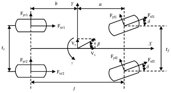
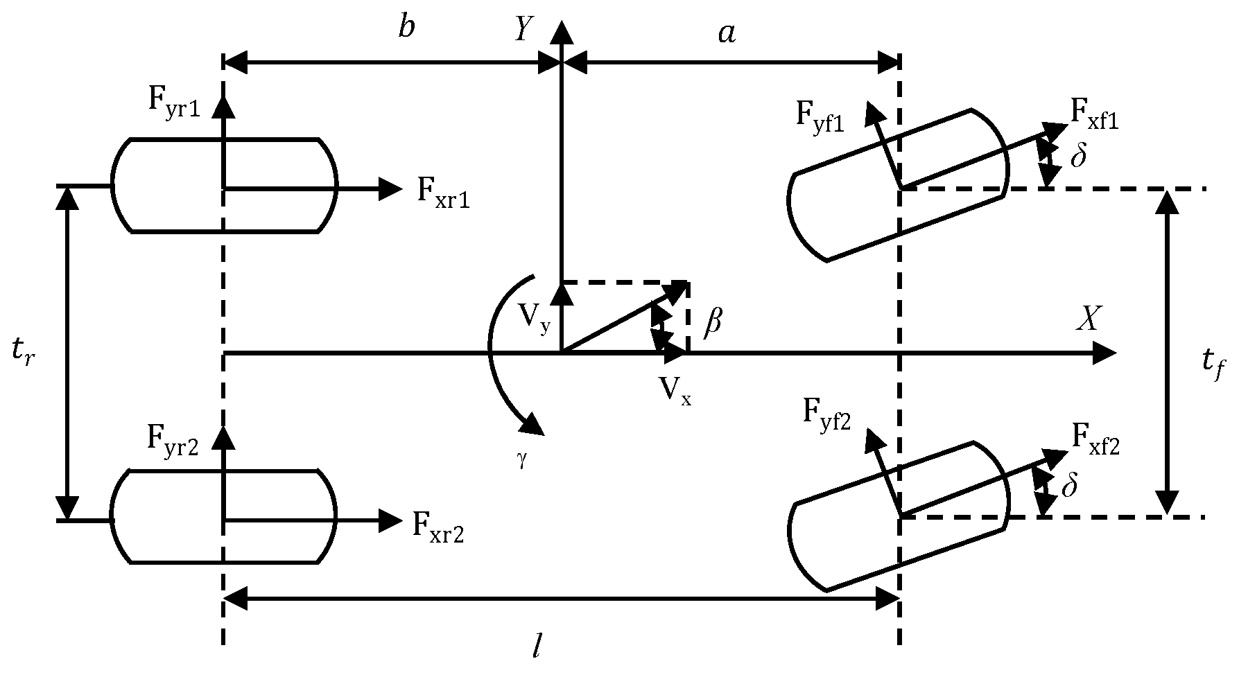
This study opts to construct a three degrees of freedom nonlinear vehicle model, illustrated in Figure 1, to address the estimation of vehicle yaw velocity and sideslip angle. The chosen model is designed to balance the intricacies of accurately describing vehicle motion behaviors while maintaining the algorithm’s real-time responsiveness to system adjustments.
Figure 1.
Three degrees of freedom vehicle model.
The mathematical model is as follows.
Lateral dynamic equation:
Longitudinal dynamic equation:
Yaw dynamics equation:
In the above formula, is the moment around the center of mass; , are, respectively, longitudinal force and lateral force; is the front wheel angle; and are the intervals from the center of mass to the front and rear axes, respectively. and are the intervals between the front and rear wheels, respectively.
The state space model of the obtained system is as follows.
According to Formulas (4) and (5), the state variable is . The control variable is . m is the vehicle equipment mass; is the yaw rate; is the sideslip angle of the center of mass; , are the lateral stiffness of the front and rear wheels, respectively. is the forward velocity; is the velocity perpendicular to the direction of travel; are longitudinal acceleration and lateral acceleration, respectively. is the axis moment of inertia.
2.1.2. Tire Model
In vehicle dynamics control, the force of an automobile tire (including lateral force, longitudinal force, and righting moment) is mainly related to load, tire pressure, and road adhesion coefficient. The tire is an important part of the automobile, and it is the part of the vehicle in direct contact with the ground. Its interaction force with the ground has an important impact on the braking performance and handling stability of the automobile. Therefore, when simulating the dynamic performance of the automobile, it is necessary to establish an accurate vehicle tire model. In the tire model, the precision of the magic tire model is high, and when the tire is in a nonlinear state, it can reflect the nonlinear characteristics of the tire more accurately. Therefore, choose the Magic tire model to show the dynamic characteristics of the tire movement. Its representation is as follows:
This is an example of the equation.
Here, is the longitudinal (lateral force) of the tire, or perhaps the torque exerted by the tire on the axis; is determined by , representing the longitudinal slip rate of the vehicle tire or the vehicle sideslip angle; is the peak factor; is the form factor; is the stiffness factor; is the vertical offset; indicates the horizontal offset. When predicting the state of the vehicle, it is necessary to calculate the transverse and longitudinal force on the tire, and the tire’s longitudinal force is
is slip rate;
Lateral force of the tire is:
where is the sideslip angle; ; . For the fitting coefficient, it can be provided by the magic tire model in Carsim software.
2.2. Symmetry-Aware Formulation of Vehicle State Estimation
For vehicle lateral dynamics, the term “symmetry-aware” refers to the use of the approximate left-right mirror symmetry of vehicle responses as a physical guideline for observer design. Under identical road adhesion, loading, and tire working conditions, the yaw-rate and sideslip-angle responses caused by positive and negative steering inputs with similar magnitudes should exhibit similar amplitudes but opposite signs. Therefore, an effective state observer is expected to provide balanced estimation performance during both left and right lateral maneuvers.
In a conventional EKF, the measurement noise covariance matrix is usually fixed. When the actual sensor noise level varies, the relative confidence between model prediction and measurement correction may become mismatched, which can cause direction-dependent estimation bias or delayed convergence. From the symmetry-aware perspective, this problem can be interpreted as a loss of statistical balance in the innovation sequence during alternating lateral motions.
Based on this consideration, the proposed CG_EKF adaptively tunes the measurement noise covariance matrix by minimizing the mismatch between the actual and theoretical innovation covariances. The chaotic search improves global exploration, while the variable-step gradient refinement accelerates local convergence. By maintaining innovation consistency through covariance adaptation, the proposed observer improves the balanced estimation of yaw rate and sideslip angle under symmetric lateral excitations.
2.3. KF Observer Based on Chaotic Gradient Descent Method
2.3.1. Principle of EKF
The general vehicle system is inherently complex and nonlinear. Traditional Kalman filters are primarily suited for linear systems and struggle with nonlinearity. The Unscented Kalman Filter maintains semidefiniteness of matrices during filtering but can become unstable and prone to collapse. The EKF linearizes nonlinear systems through Taylor expansion, but may suffer from inaccuracies due to neglecting higher-order terms. Second-order EKF improves accuracy but increases computational complexity, limiting its practical use. Therefore, this paper employs an improved EKF algorithm to mitigate nonlinear measurement errors in vehicle state estimation. This approach ensures observation errors are within acceptable limits while considering real-time constraints of the observation system.
Vehicle differential equation of three degrees of freedom:
where, is the state quantity; is the control variable; is the observed quantity; are independent inherent noise and observed noise, with variances of and , respectively.
EKF filtering is a recursive iterative process, which is suitable for the discretization of time series and requires the discretization of the vehicle’s 3-degree-of-freedom equation. The discretized state equation is obtained by the forward Euler method:
where and are respectively the partial derivatives of the state vector after linearization of the equation.
Assigning initial values to the linearized state and observation equations and recursive estimation of the EKF, so that the input of the model is . The algorithm process of EKF is as follows:
Prediction:
Update:
2.3.2. KF Filter Based on Chaotic Gradient Algorithm
Based on the symmetry-aware formulation discussed above, the key issue is to maintain the consistency between the actual innovation statistics and the theoretical innovation covariance during vehicle lateral motion. Therefore, the measurement noise covariance matrix is adaptively optimized in the proposed CG_EKF.
The variance of system noise and observed noise is in an uncertain environment during vehicle operation. The process noise and measurement noise change in real time. The conventional EKF algorithm assumes that the observation noise does not change in the filtering process, but this will affect the filtering accuracy to some extent. Therefore, it is necessary to find the optimal value of these two noise covariances in the process of system motion. When adjusting the covariance matrix in the Kalman filter, the simultaneous adjustment of and will make the filtering process easily diverge; therefore, this paper only updates the measurement noise covariance matrix , while the process noise covariance matrix is kept fixed.
is the estimate of the observed noise variance at time.
, and the relationship between time and the estimate at time is as follows:
where is the fitness coefficient.
The error of the variance of innovation [27] at time , that is, the true variance minus the theoretical variance, is equal to :
In the equation, is the true variance of the innovation;
is the theoretical variance of the new information.
The new spread ’s square is the objective function we need, find its minimum value for the target optimization.
The CG_EKF algorithm principle in this paper is as follows:
In order to ensure that the search is carried out quickly, the forward difference method is used to calculate the gradient:
where, is the number of iterations, the gradient vector at the kth iteration is adaptively obtained by the difference method, which is suitable for any functional form; is the iteration step size; in the search process, make , and = 0.9 if the value of the objective function decreases; otherwise = 1.1, which ensures that the gradient descent is relatively smooth. These two values were selected to provide a conservative adjustment of the search step. If the scaling factor is too large, the search process may oscillate or overshoot near the optimum; if it is too small, the step-size adaptation may become insensitive, and the convergence speed may decrease. Therefore, a 10% decrease or increase is adopted to balance convergence stability and optimization efficiency.
The convergence condition of the gradient descent method is:
is a given positive number.
Let the optimal solution obtained by the variable scale gradient descent search be , and the range of values of the optimization variables be set as:
where defines a small local search region around the solution obtained by the gradient method. This conservative setting helps improve local search efficiency and avoids unnecessary wide-range exploration at the beginning, is the variable scale sign, and the independent variables take the values .
When , then ; when , then . The search scope is searched from 10% of the original scope. Mapping linearly between [0, 1] according to the range of variables. From , we obtain a chaotic sequence , . is the chaos variable, is the number of iterations, is the coefficient.
Transform each of the chaotic variables into the original variables so that they are chaotic variables.
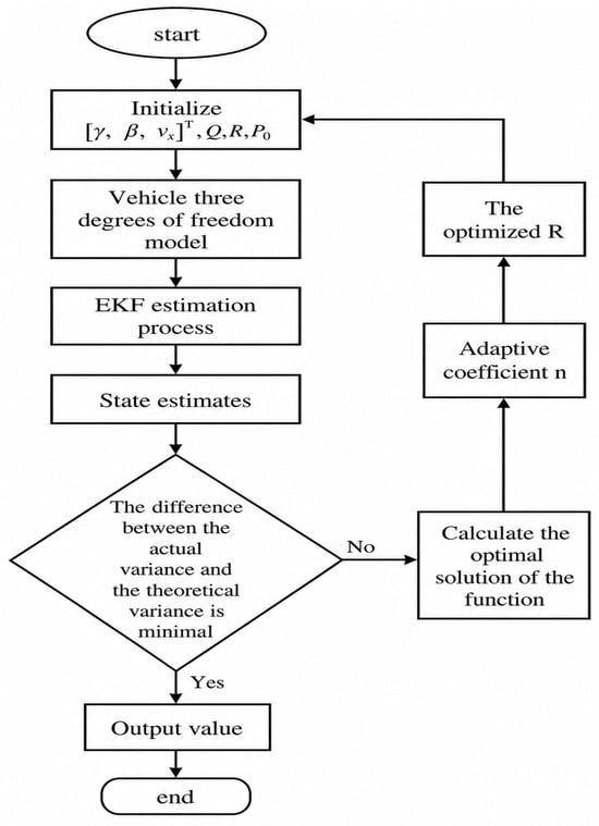
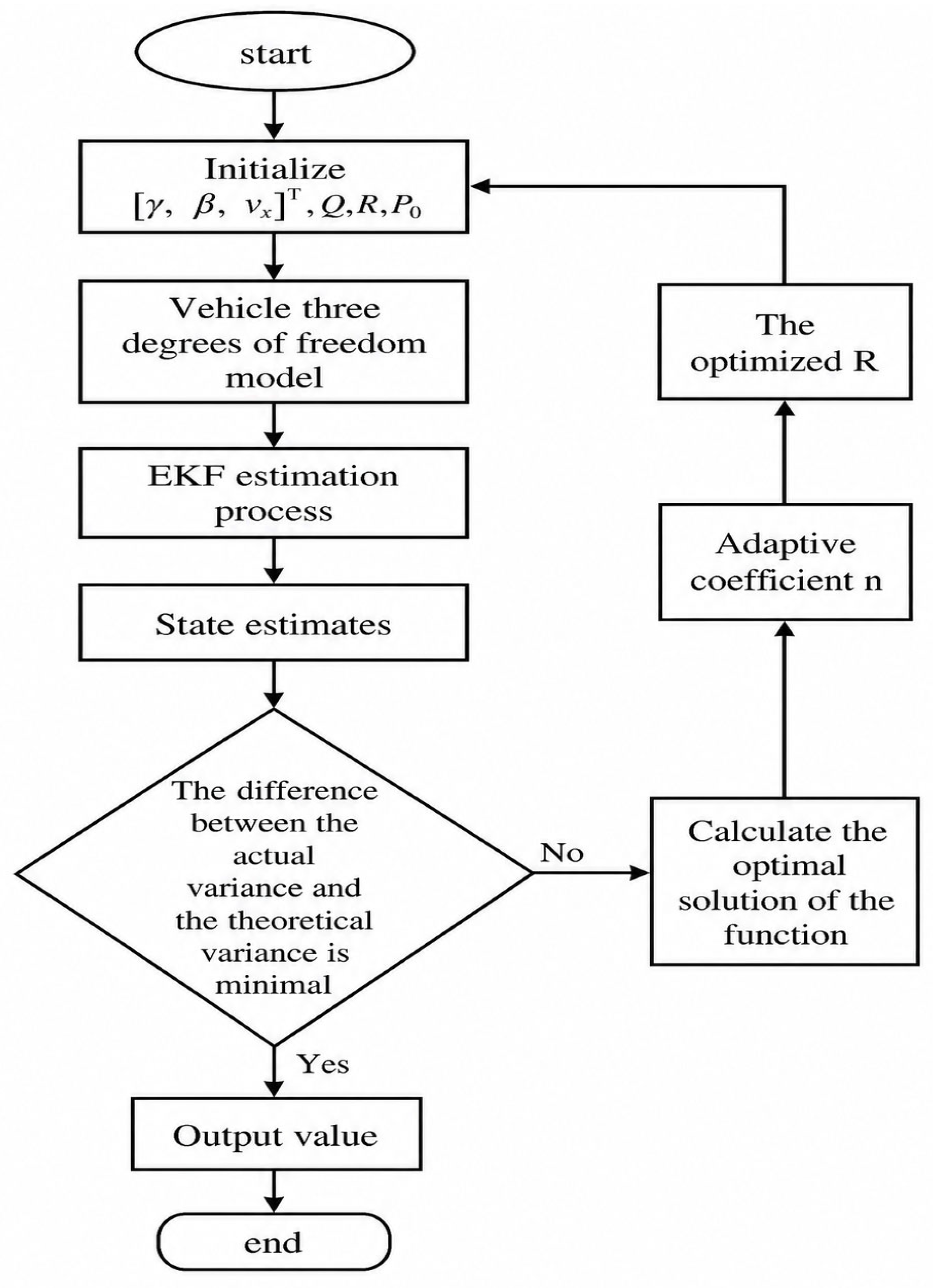
As shown in Figure 2, let the optimization point obtained by the gradient method be , the corresponding objective function value should be . The search is performed with the chaotic variable obtained after the transformation.
Figure 2.
Block diagram of algorithm workflow.
Step 1: If the function value , then , , terminate this search and exit.
Step 2: Otherwise, drop and let , if then turn to Equation (21) and search again, otherwise proceed to the next step.
Step 3: If this search fails to find a new optimization point, replace with , then repeat the above steps and start the chaotic search again. After ten searches, is unchanged or is unchanged, and the optimization is finished.
The flow chart of the algorithm proposed in this paper is shown as follows.
3. The Simulation Experiment
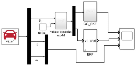
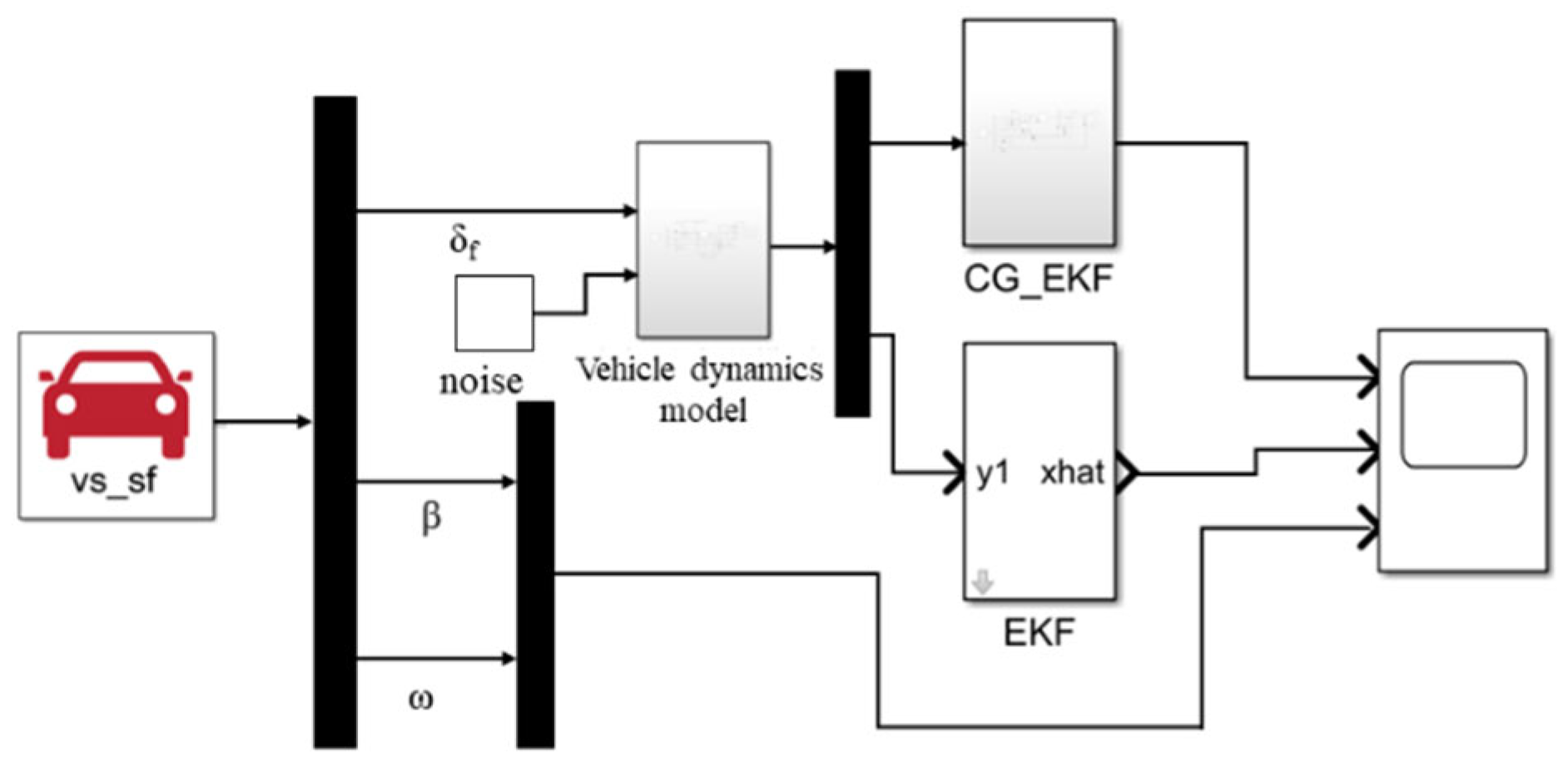
Carsim 2020.0 and MATLAB/Simulink R2021b software were used for joint experimental simulation to verify the applicability of the proposed CG_EKF algorithm in vehicle state estimation. Specifically, Carsim is responsible for outputting the parameters required by the CG_EKF algorithm and simulating the sensor measurement parameters, which are input into the Simulink simulation module. Simulink processes the data and calculates the state estimation by the CG_EKF state estimator. In practice, the sensors are affected by noise. Therefore, bounded random measurement noise was added to the observation system. Specifically, each sensor observation was set as the CarSim output value plus a uniformly distributed random disturbance within ±10% of the current value. The noise was added only to the observation signals rather than to the reference vehicle states, so as to simulate the uncertainty of sensor measurements. Setting up the noise in this way facilitates a more realistic simulation of sensor operation in real-world applications. The state quantity selected in this paper is , and the state quantity selected for the required estimation is . According to the national passenger car test standards [28], the experimental speed was set to 70 the Double-lane-change condition and 60 for the Slalom condition, and pavement adhesion coefficients are all 0.8. The co-simulation model built is shown in Figure 3.
Figure 3.
Block diagram of the working structure of the vehicle state estimation mode.
It should be noted that both the double-lane-change and slalom maneuvers involve alternating left and right steering excitations. Therefore, these two conditions are suitable for examining not only the overall estimation accuracy but also the estimation consistency under approximately symmetric lateral responses. In this study, the estimation performance is evaluated using MAE and RMSE of yaw rate and sideslip angle, which reflect the average estimation deviation and the overall error fluctuation, respectively.
In addition to the proposed CG_EKF, EKF, UKF, and AEKF were introduced as benchmark observers for comparison. All four observers were evaluated under the same vehicle model, input conditions, and measurement noise settings. The EKF serves as the basic nonlinear filtering benchmark, the UKF represents a sigma-point-based nonlinear filtering method, and the AEKF represents a conventional adaptive covariance adjustment strategy. The following analysis, therefore, compares the estimation performance of EKF, UKF, AEKF, and CG_EKF under the same test conditions. The vehicle parameters are shown in Table 1. The AEKF benchmark was implemented with reference to the adaptive extended Kalman filtering strategy reported in Qi et al. [11].
Table 1.
Vehicle-related parameters.
Table 2 compares the estimation errors of EKF, UKF, AEKF, and the proposed CG_EKF for yaw rate and sideslip angle under the two maneuvers. It can be seen that CG_EKF achieves the lowest MAE and RMSE in all test cases, indicating that the chaotic-gradient covariance optimization provides better estimation accuracy than the three benchmark observers. Since the selected maneuvers contain positive and negative lateral excitation phases, the consistently smaller errors also support the symmetry-aware design motivation of maintaining balanced estimation performance under left and right steering responses.
Table 2.
Error comparison of different observers under double-lane-change and slalom conditions.
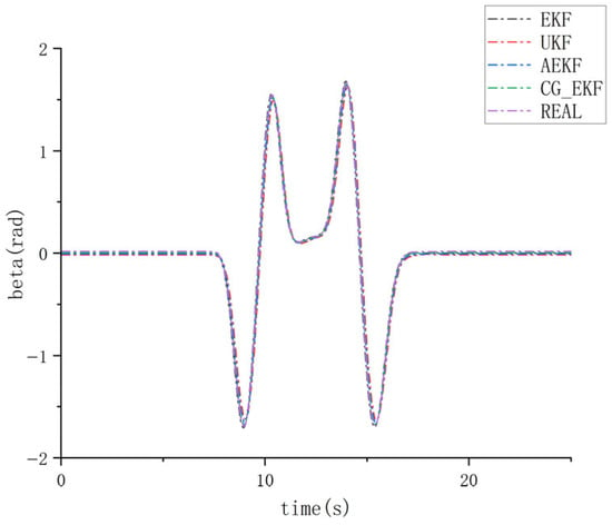
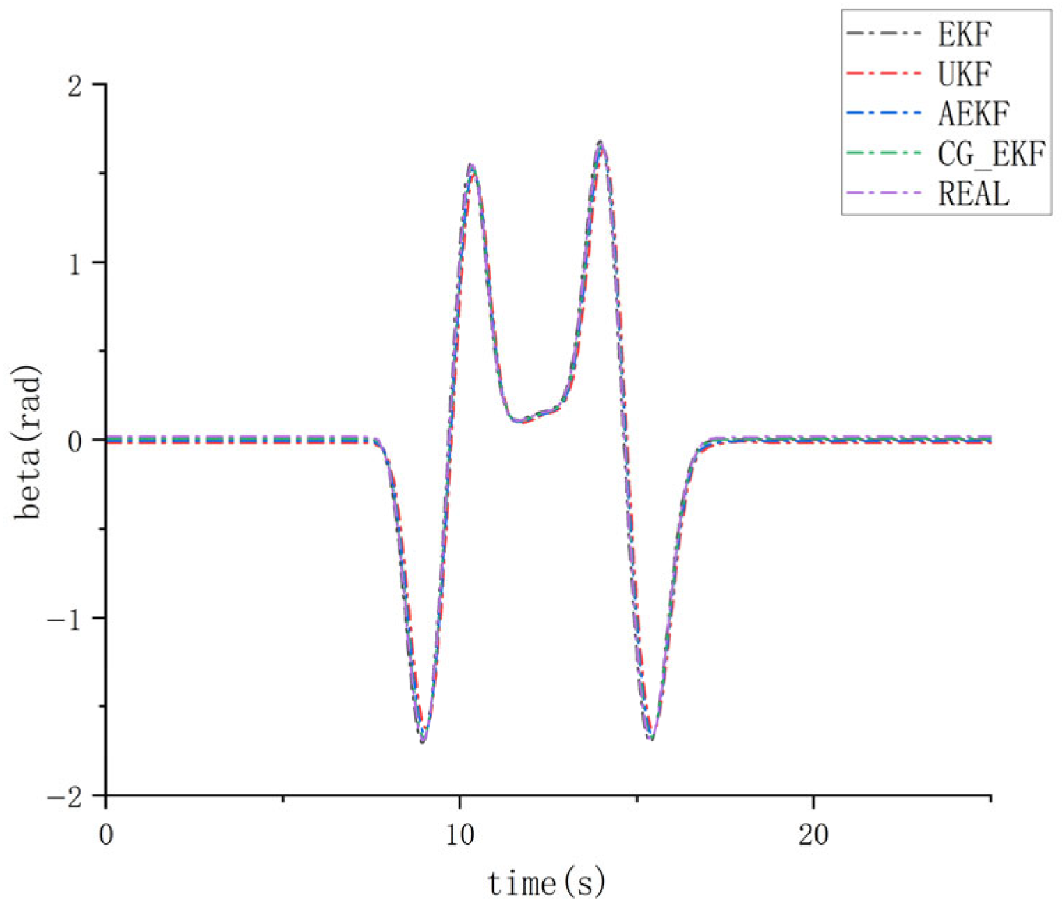
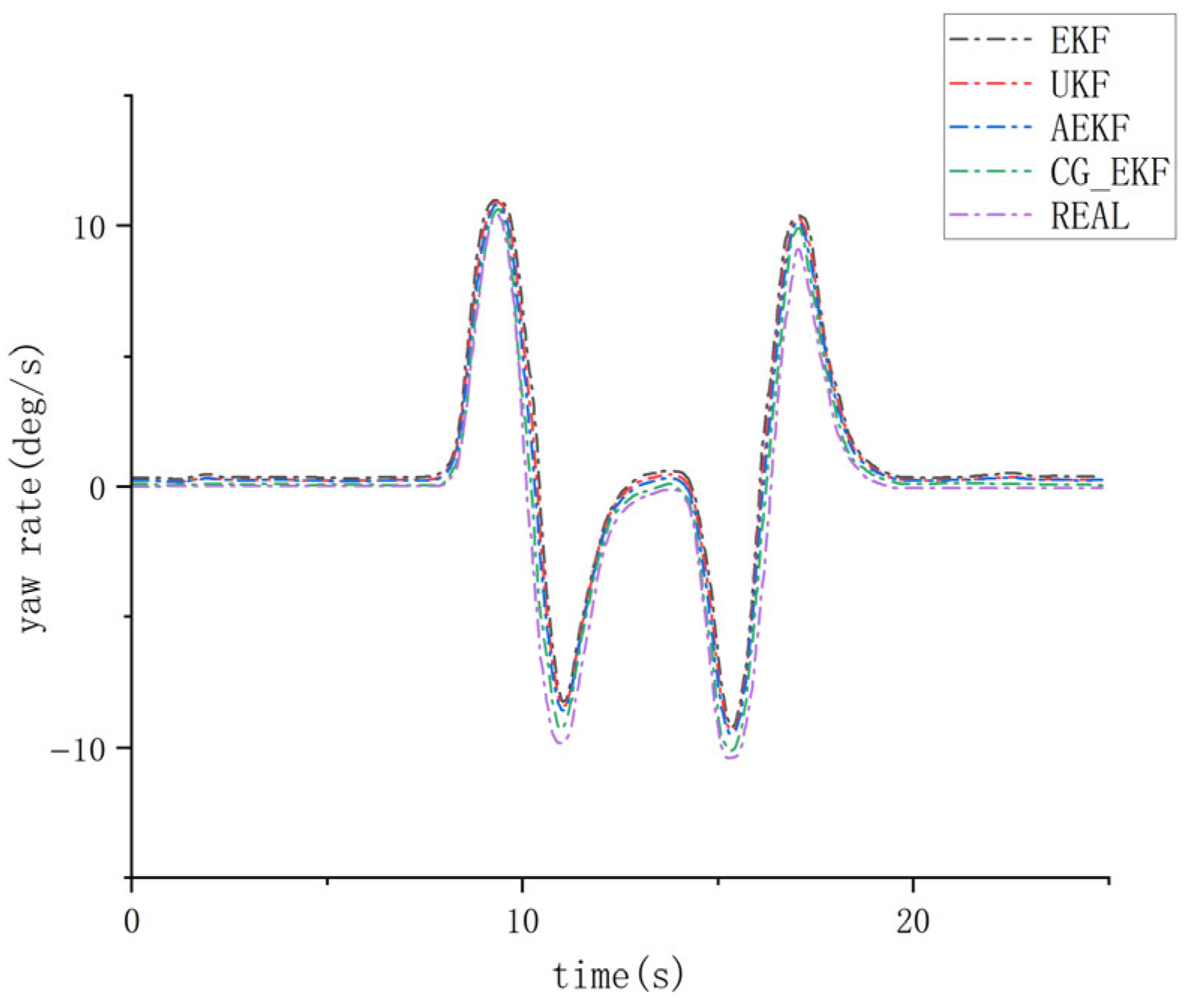
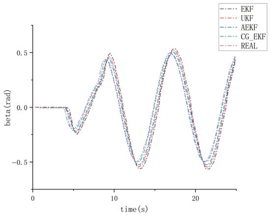
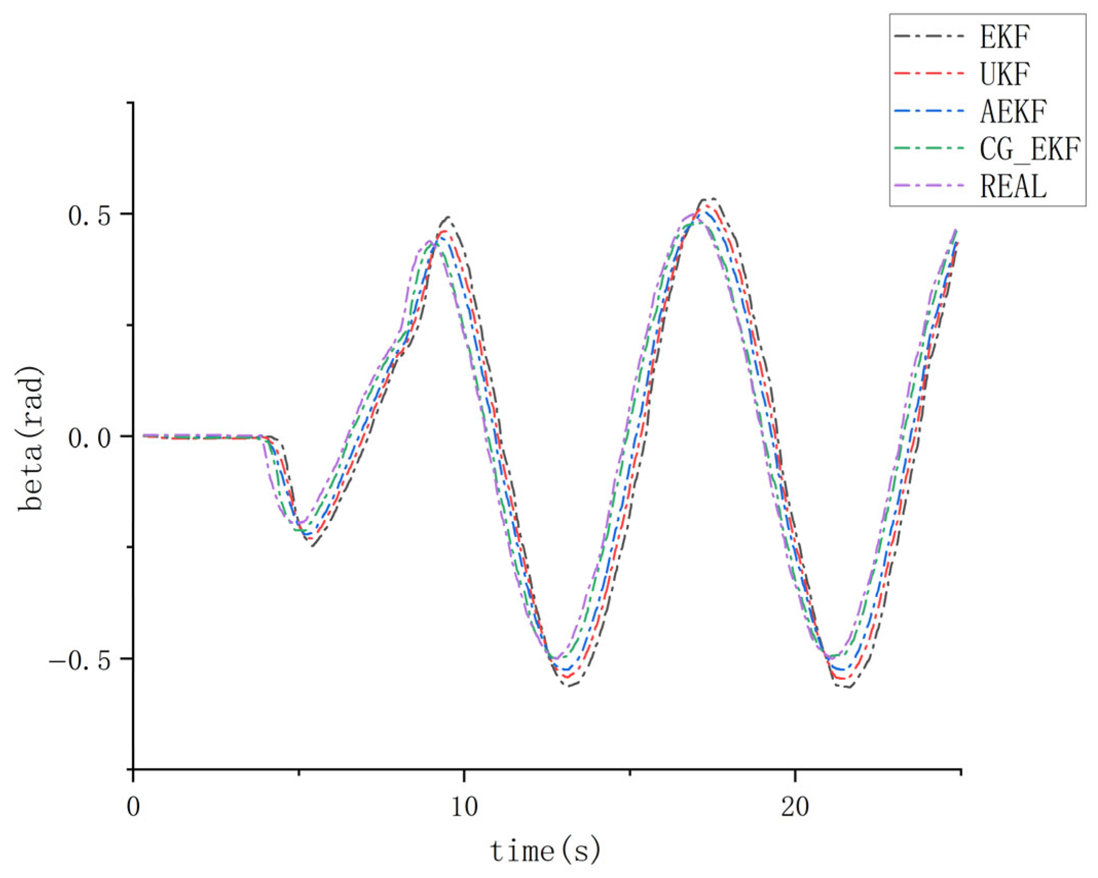
Under the double-lane-change condition, Figure 4 and Figure 5 show the estimation results of sideslip angle and yaw rate, respectively. For sideslip angle estimation, CG_EKF obtains MAE/RMSE values of 0.0278 and 0.0494, achieving reductions of 69.0%/61.1%, 61.2%/54.2%, and 45.8%/36.8% compared with EKF, UKF, and AEKF, respectively. For yaw-rate estimation, CG_EKF achieves MAE/RMSE values of 0.1501 and 0.1795, reducing the corresponding errors by 66.7%/65.7%, 62.7%/60.1%, and 53.0%/52.7% compared with EKF, UKF, and AEKF, respectively. These results demonstrate that the proposed CG_EKF provides consistently better estimation accuracy than the three benchmark observers under the double-lane-change condition.
Figure 4.
Sideslip-angle estimation under the double-lane-change condition.
Figure 5.
Yaw-rate estimation under the double-lane-change condition.
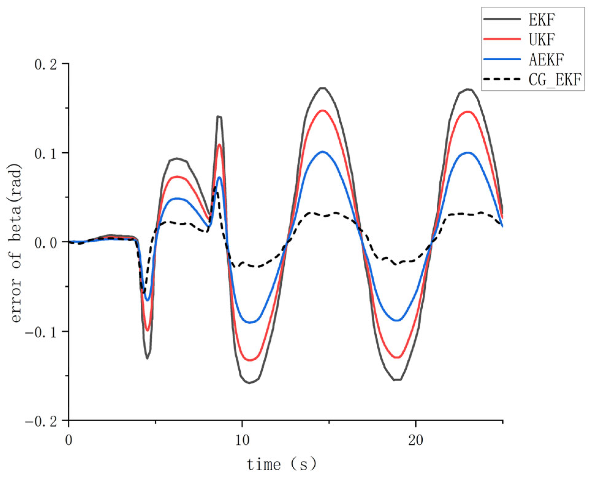
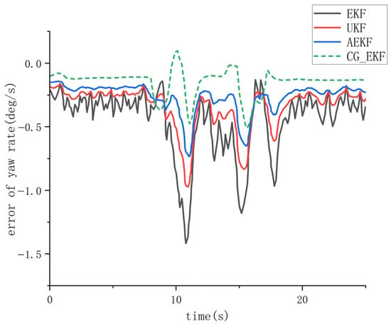
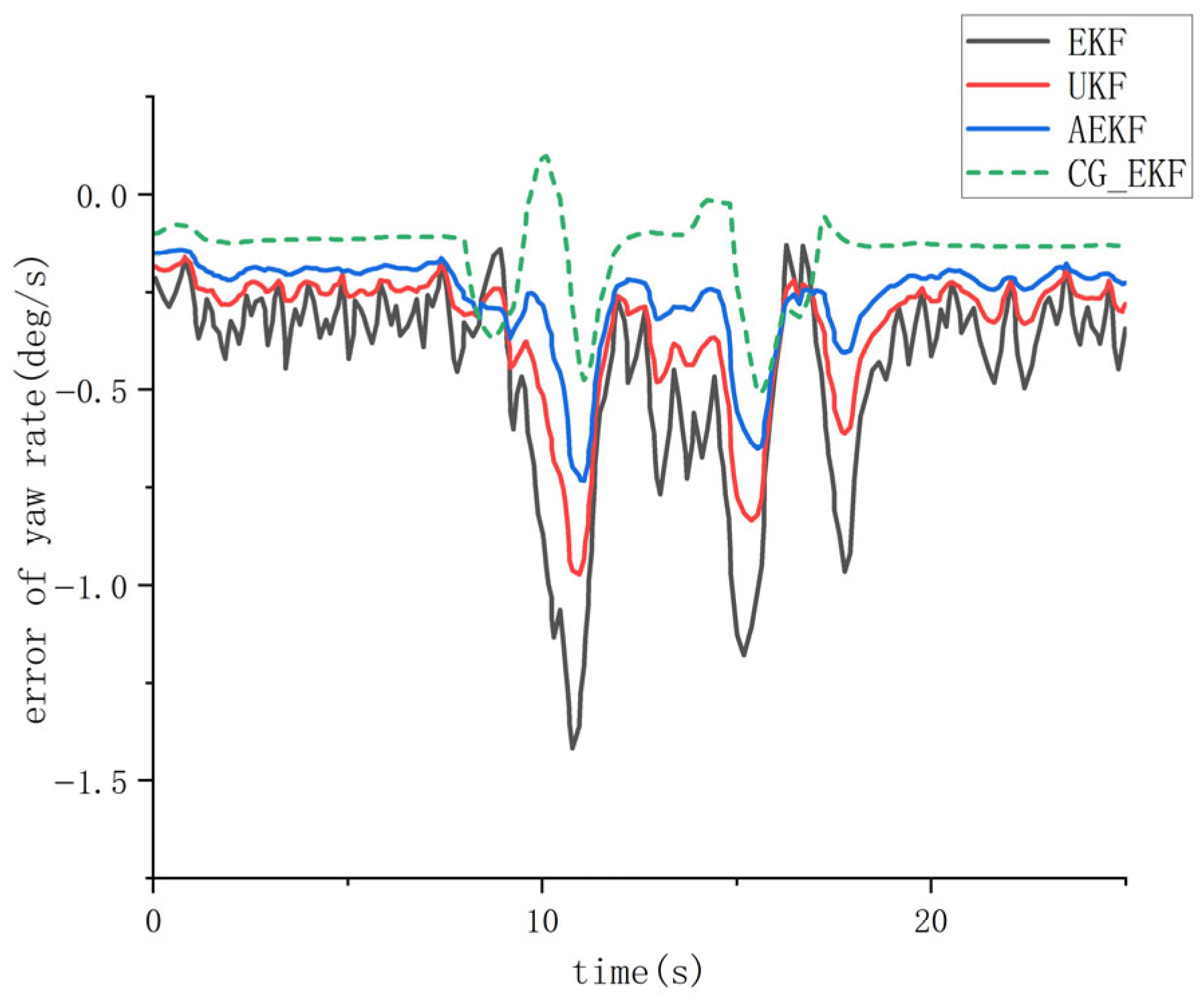
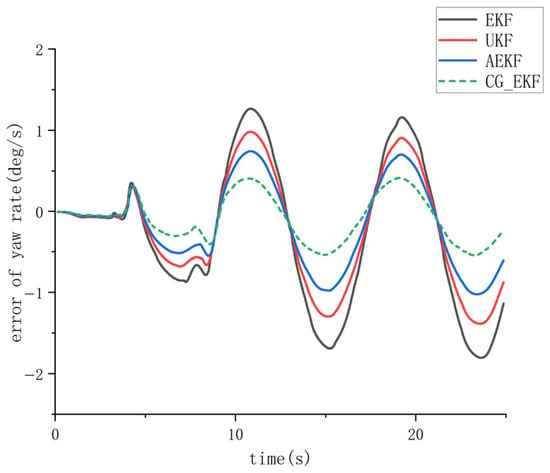
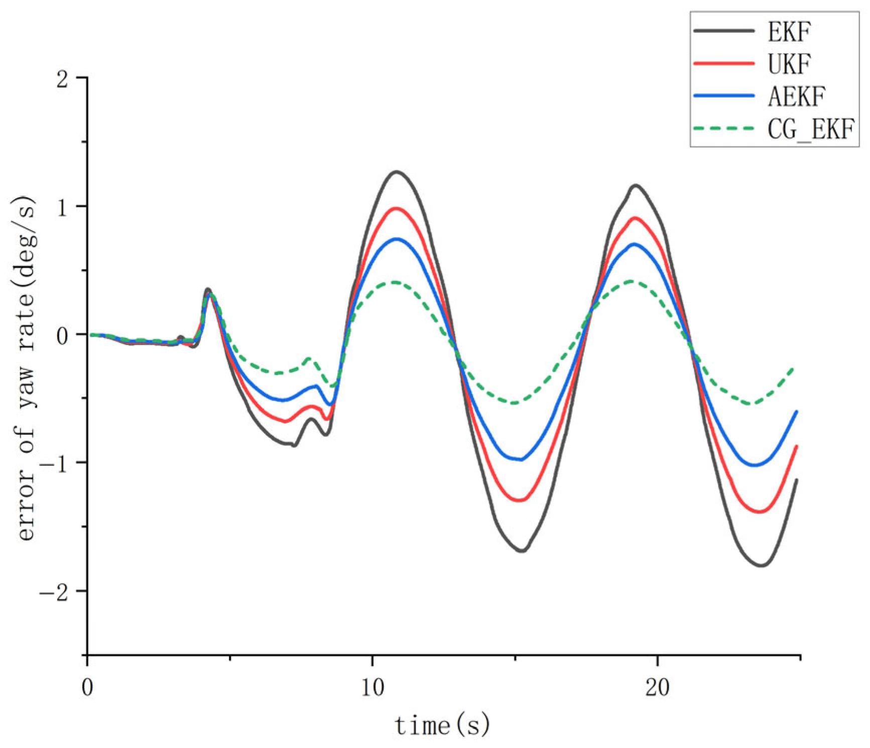
Figure 6 and Figure 7 show the estimation errors of sideslip angle and yaw rate under the double-lane-change condition, respectively. For the sideslip angle estimation error, CG_EKF presents the smallest fluctuation range among the four methods, especially during rapid steering transitions and state sign-changing phases. Compared with EKF, UKF, and AEKF, the error curve of CG_EKF remains closer to zero, indicating better error suppression capability. For the yaw-rate estimation error, CG_EKF also shows a smaller error amplitude than the other three observers. The error peaks mainly appear near rapid steering transitions, where tire nonlinearities and model linearization errors become more significant.
Figure 6.
Sideslip-angle error under the double-lane-change condition.
Figure 7.
Yaw-rate error under the double-lane-change condition.
This demonstrates that the proposed chaotic-gradient covariance optimization can effectively reduce error peaks and improve convergence stability under the double-lane-change condition.
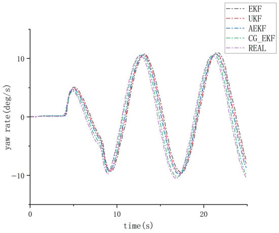
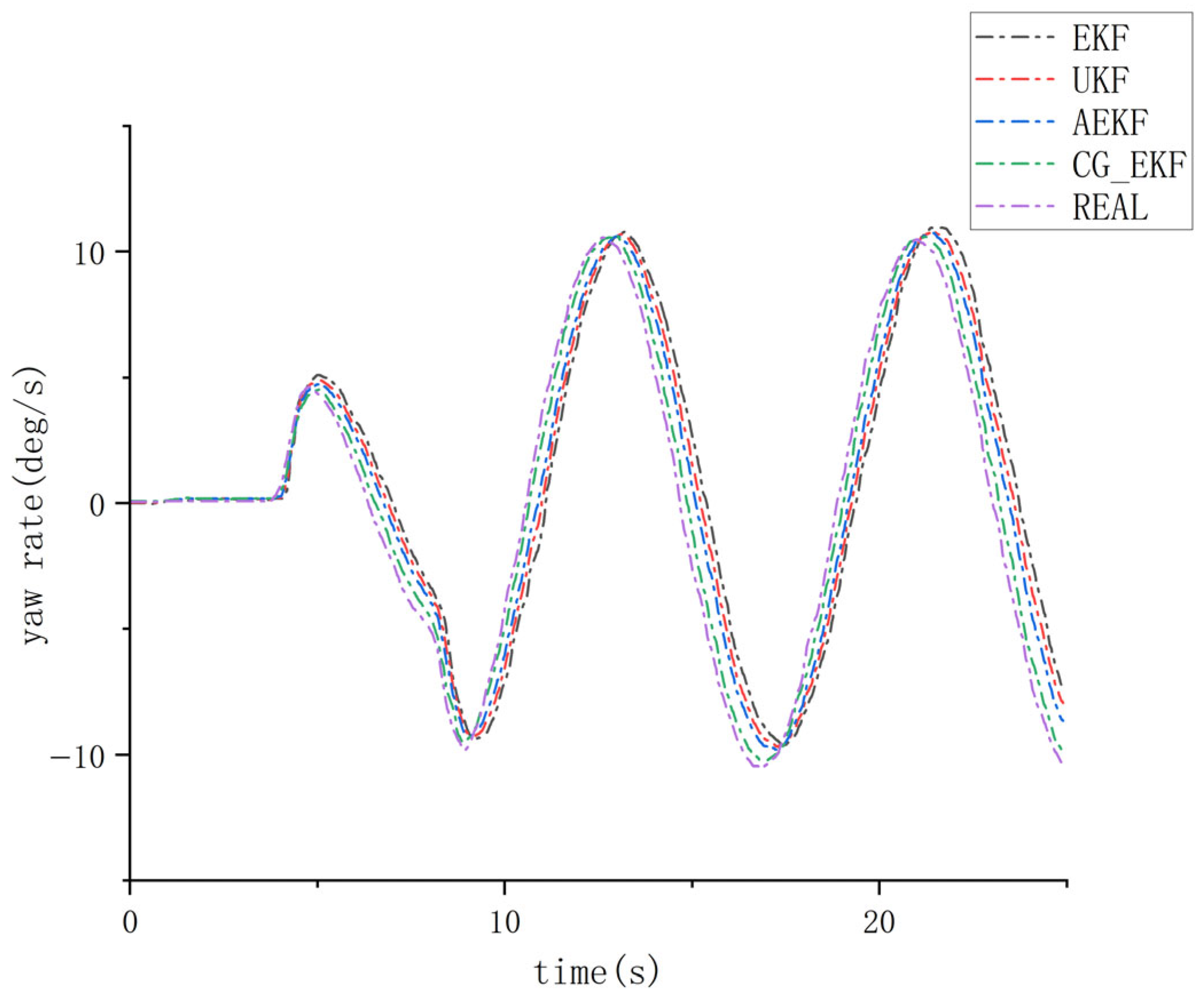
Under the slalom condition, Figure 8 and Figure 9 show the estimation results of sideslip angle and yaw rate, respectively. For sideslip angle estimation, CG_EKF obtains MAE/RMSE values of 0.0195 and 0.0231, achieving reductions of 77.6%/77.9%, 71.7%/71.9%, and 62.6%/61.0% compared with EKF, UKF, and AEKF, respectively. For yaw-rate estimation, CG_EKF achieves MAE/RMSE values of 0.2565 and 0.3038, reducing the corresponding errors by 65.9%/67.2%, 56.5%/57.8%, and 47.7%/52.9% compared with EKF, UKF, and AEKF, respectively. These results indicate that the proposed CG_EKF maintains the best estimation accuracy among the four observers under continuous left-right steering excitation.
Figure 8.
Sideslip-angle estimation under the slalom condition.
Figure 9.
Yaw-rate estimation under the slalom condition.
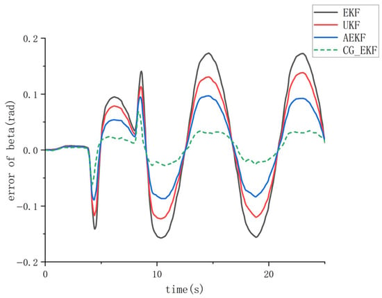
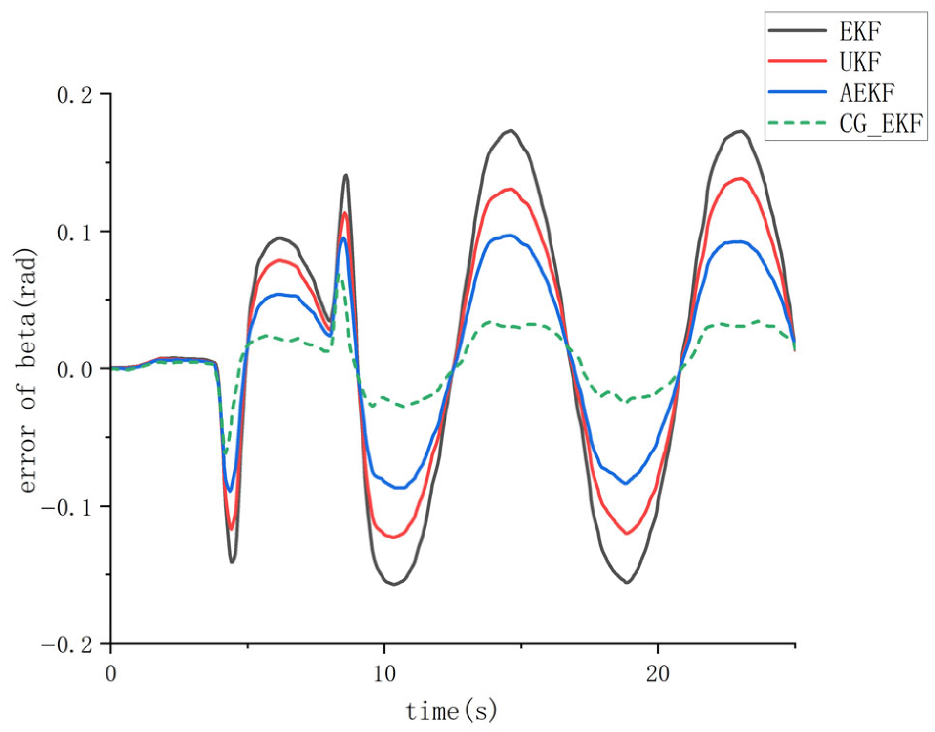
Figure 10 and Figure 11 show the estimation errors of sideslip angle and yaw rate under the slalom condition, respectively. Since the slalom maneuver contains repeated steering reversals, the observer needs to maintain stable estimation performance during continuous positive and negative lateral responses. Compared with EKF, UKF, and AEKF, the error curves of CG_EKF remain closer to zero and show smaller fluctuation amplitudes in both sideslip-angle and yaw-rate estimation. This indicates that the proposed chaotic-gradient covariance optimization can effectively suppress error accumulation during periodic steering transitions and improve the convergence stability of vehicle state estimation.
Figure 10.
Sideslip-angle error under the slalom condition.
Figure 11.
Yaw-rate error under the slalom condition.
4. Conclusions
This paper proposed a symmetry-aware vehicle state estimation method based on a chaotic-gradient-optimized extended Kalman filter for yaw-rate and sideslip-angle estimation. The symmetry-aware motivation was derived from the approximate mirror symmetry of vehicle lateral dynamics under left and right steering excitations. To maintain statistical consistency under stochastic disturbances, the innovation covariance mismatch was used as the optimization objective for adaptive measurement noise covariance tuning.
The proposed CG_EKF combines chaotic search and variable-step gradient refinement to optimize the measurement noise covariance matrix. In this way, the observer improves the consistency between theoretical and actual innovation covariances and enhances the balance between model prediction and measurement correction.
The CarSim and MATLAB/Simulink co-simulation results under double-lane-change and slalom conditions show that CG_EKF achieves lower MAE and RMSE than EKF, UKF, and AEKF in yaw-rate and sideslip-angle estimation. The results indicate that the proposed method improves both estimation accuracy and balanced estimation performance under alternating left-right lateral maneuvers.
Author Contributions
Conceptualization, Q.C. and W.L.; methodology, Q.C. and W.L.; software, Q.C.; validation, Q.C., W.L., X.L. and H.C.; data curation, Q.C.; writing—original draft preparation, Q.C.; writing—review and editing, Q.C., W.L., X.L., H.C. and B.D.; visualization, Q.C.; supervision, W.L. All authors have read and agreed to the published version of the manuscript.
Funding
This research received no external funding.
Data Availability Statement
The original contributions presented in this study are included in the article. Further inquiries can be directed to the corresponding author.
Acknowledgments
The authors gratefully acknowledge the technical support and assistance provided during the experiment. Thanks are also due to the anonymous reviewers for their valuable comments and suggestions to improve the quality of the paper.
Conflicts of Interest
The authors declare no conflicts of interest.
References
- Wang, X.; You, Z.; Zhao, K. Inertial/celestial-based fuzzy adaptive unscented Kalman filter with covariance intersection algorithm for satellite attitude determination. Aerosp. Sci. Technol. 2016, 48, 214–222. [Google Scholar] [CrossRef] [Scilit]
- Xue, X. Distributed drive electric vehicle state estimation based on extended Kalman filter. Energy Procedia 2016, 104, 538–543. [Google Scholar] [CrossRef] [Scilit]
- Chu, W.; Luo, Y.; Dai, Y.; Li, K. In-wheel motor electric vehicle state estimation by using unscented particle filter. Veh. Des. 2015, 67, 117–135. [Google Scholar] [CrossRef] [Scilit]
- Wang, Y.; Wang, J.; Yu, Q. Soft measurement of intelligent vehicle side-slip angle based on extended Kalman filter. J. Phys. Conf. Ser. 2020, 1635, 012028. [Google Scholar] [CrossRef] [Scilit]
- Sun, W.; Wang, Z.; Wang, J.; Wang, X.; Liu, L. Research on a real-time estimation method of vehicle sideslip angle based on EKF. Sensors 2022, 22, 3386. [Google Scholar] [CrossRef] [Scilit]
- Wenzel, T.A.; Burnham, K.J.; Blundell, M.V.; Williams, R.A. Dual extended Kalman filter for vehicle state and parameter estimation. Veh. Syst. Dyn. 2006, 44, 153–171. [Google Scholar] [CrossRef] [Scilit]
- Reina, G. Vehicle parameter estimation using a model-based estimator. Mech. Syst. Signal Process. 2016, 87, 227–241. [Google Scholar] [CrossRef] [Scilit]
- Katriniok, A.; Abel, D. Adaptive EKF-based vehicle state estimation with online assessment of local observability. IEEE Trans. Control Syst. Technol. 2016, 24, 1368–1381. [Google Scholar] [CrossRef] [Scilit]
- Wang, Y.; Xu, L.; Zhang, F.; Dong, H.; Liu, Y.; Yin, G. An adaptive fault-tolerant EKF for vehicle state estimation with partial missing measurements. IEEE/ASME Trans. Mechatron. 2021, 26, 1318–1327. [Google Scholar] [CrossRef] [Scilit]
- Hrgetic, M.; Deur, J.; Pavkovic, D.; Barber, P. Adaptive EKF-based estimator of sideslip angle using fusion of inertial sensors and GPS. SAE Int. 2011, 4, 700–712. [Google Scholar] [CrossRef] [Scilit]
- Qi, D.; Feng, J.; Wan, W.; Song, B. A novel maximum correntropy adaptive extended Kalman filter for vehicle state estimation under non-Gaussian noise. Meas. Sci. Technol. 2023, 34, 025114. [Google Scholar] [CrossRef] [Scilit]
- Wang, Z.; Chen, C.; Jiang, Q.; Zheng, H.; Kaku, C. State estimation of drive-by-wire chassis vehicle based on dual unscented particle filter algorithm. Chin. J. Mech. Eng. 2024, 37, 11. [Google Scholar] [CrossRef] [Scilit]
- Zha, Y.; Liu, X.; Ma, F.; Liu, C. Vehicle state estimation based on extended Kalman filter and radial basis function neural networks. Int. J. Distrib. Sens. Netw. 2022, 18, 6. [Google Scholar] [CrossRef] [Scilit]
- Jin, X.; Yang, J.; Xu, L.; Wei, C.; Wang, Z.; Yin, G. Combined estimation of vehicle dynamic state and inertial parameter for electric vehicles based on dual central difference Kalman filter method. Chin. J. Mech. Eng. 2023, 36, 91. [Google Scholar] [CrossRef] [Scilit]
- Kumar, N.R.; Nagabhooshanam, E. EKF with artificial bee colony for precise positioning of UAV using global positioning system. IETE J. Res. 2021, 67, 60–73. [Google Scholar] [CrossRef] [Scilit]
- Ben Lazreg, M.; Jemmali, S.; Manai, B.; Hamouda, M. Enhanced EKF and SVSF for state of charge estimation of Li-ion battery in electric vehicle using a fuzzy parameters model. IET Electr. Syst. Transp. 2022, 12, 315–329. [Google Scholar] [CrossRef] [Scilit]
- Kim, T.; Park, T.-H. Extended Kalman filter (EKF) design for vehicle position tracking using reliability function of radar and lidar. Sensors 2020, 20, 4126. [Google Scholar] [CrossRef] [Scilit]
- Kim, D.; Min, K.; Kim, H.; Huh, K. Vehicle sideslip angle estimation using deep ensemble-based adaptive Kalman filter. Mech. Syst. Signal Process. 2020, 144, 106862. [Google Scholar] [CrossRef] [Scilit]
- Slimi, H.; Sentouh, C.; Mammar, S.; Nouveliere, L.; Arioui, H.; Merzouki, R.; Abbassi, H.A. Sensor position identification and vehicle state estimation using the extended Kalman filter. In Proceedings of the 1st Mediterranean Conference on Intelligent Systems and Automation (CISA 08), Annaba, Algeria, 30 June–2 July 2008; AIP Conference Proceedings. pp. 41–46. [Google Scholar]
- Gao, B.L.; Chen, H.; Xie, S.G.; Gong, J.F. State estimation for 4WD in-wheel motor electric vehicle. Appl. Mech. Mater. 2014, 610, 147–155. [Google Scholar] [CrossRef] [Scilit]
- Sharma, A.K.; Bouteldja, M.; Cerezo, V. Vehicle dynamic state observation and rolling resistance estimation via unknown input adaptive high-gain observer. Mechatronics 2021, 79, 102658. [Google Scholar] [CrossRef] [Scilit]
- Chen, Y.; Huang, Y.; Song, Z. Vehicle state estimation by integrating the recursive least squares method with a variable forgetting factor with an adaptive iterative extended Kalman filter. World Electr. Veh. J. 2024, 15, 399. [Google Scholar] [CrossRef] [Scilit]
- Li, J.; Feng, B.; Zhang, L.; Luo, J. Research on vehicle stability control based on a union disturbance observer and improved adaptive unscented Kalman filter. Electronics 2024, 13, 3220. [Google Scholar] [CrossRef] [Scilit]
- Chen, X.; Cheng, X. RBCKF-based vehicle state estimation by adaptive weighted fusion strategy considering composite-state tire model. World Electr. Veh. J. 2024, 15, 517. [Google Scholar] [CrossRef] [Scilit]
- Alshawi, A.; De Pinto, S.; Stano, P.; van Aalst, S.; Praet, K.; Boulay, E.; Ivone, D.; Gruber, P.; Sorniotti, A. An adaptive unscented Kalman filter for the estimation of the vehicle velocity components, slip angles, and slip ratios in extreme driving manoeuvres. Sensors 2024, 24, 436. [Google Scholar] [CrossRef] [Scilit] [PubMed]
- Wu, L.; Wang, W.; Li, P.; Zhu, Y. Vehicle sideslip angle estimation using deep reinforcement learning combined with unscented Kalman filter. Sensors 2025, 25, 7489. [Google Scholar] [CrossRef] [Scilit]
- Zhang, F.; Wei, M.; Zhao, W. Vehicle state estimation based on ant colony optimization UKF algorithm. China Mech. Eng. 2015, 26, 3046–3050. [Google Scholar]
- GB/T 40521.1-2021; Passenger Cars Test Track for a Severe Lane-Change Manoeuvre—Part 1: Double Lane-Change. Standards Press of China: Beijing, China, 2021.

Disclaimer/Publisher’s Note: The statements, opinions and data contained in all publications are solely those of the individual author(s) and contributor(s) and not of MDPI and/or the editor(s). MDPI and/or the editor(s) disclaim responsibility for any injury to people or property resulting from any ideas, methods, instructions or products referred to in the content. |
© 2026 by the authors. Licensee MDPI, Basel, Switzerland. This article is an open access article distributed under the terms and conditions of the Creative Commons Attribution (CC BY) license.