Article

A Brown Bear Optimization Driven RGB–Sobel Histogram Fusion Approach for Robust Color Image Segmentation

by
Dussa Sudha Mohan
* and
Kothapelli Punnam Chandar
Department of Electronics and Communication Engineering, Kakatiya University, Warangal 506009, Telangana, India
*
Author to whom correspondence should be addressed.
Symmetry 2026, 18(5), 795; https://doi.org/10.3390/sym18050795
Submission received: 6 March 2026 / Revised: 15 April 2026 / Accepted: 28 April 2026 / Published: 6 May 2026

Abstract

Image segmentation is the first step of image processing. It allows us to comprehend and extract information from the digital image. Multilevel thresholding is one of the most commonly used image segmentation techniques because of its simplicity and effectiveness. However, with the higher threshold level required, the more complex the process of finding the optimal threshold values becomes more complex. In this research, an effective optimization-based image segmentation technique using Otsu’s multilevel thresholding technique as the objective function to overcome the difficulties of finding the best threshold values is proposed. Instead of using the exhaustive search process, which requires more time, the best threshold values are obtained using different optimization techniques based on the nature of the image. In this study, the optimized threshold values are computed based on Otsu’s scheme, Sobel filter with Brown Bear Optimization Algorithm (BBOA), which is compared with thresholds computed based on the Artificial Bee Colony (ABC) algorithm, Jaya Algorithm (JA), Moth Flame Optimization (MFO) algorithm, Whale Optimization Algorithm (WOA) algorithm, and Particle Swarm Optimization (PSO) algorithm for segmentation. The objective function includes the sum of the variances of all four channels, namely, Red, Green, Blue, and Gray (Sobel). The superiority of the proposed method (BBOA_S) is tested on ten natural color benchmark images to verify results, and the quality of the suggested method is evaluated quantitatively by applying popular image quality assessment parameters, including PSNR, SSIM, and FSIM. The experimental results clearly show the efficiency of the suggested method of segmentation. In fact, the suggested method of segmentation has a higher PSNR value, up to 26.11, compared to other optimization methods, which have lower values. Similarly, the suggested method has a high value of structural similarity, up to 0.988, indicating that it performs a great job in terms of structural similarity. The proposed method also highly minimizes the reconstruction error, as indicated by the minimum values of the MSE, which are close to 194. This is better compared to the results of most of the other methods, which were carried out on the same images. Although the FSIM values of the proposed method are comparable to the values of the other methods, it is evident that the proposed method is good and reliable, as indicated by the overall quantitative and visual assessment. Therefore, it is clear that the use of Otsu’s multi-layer thresholding and the Sobel filter effect in combination with BBOA is effective and good.

1. Introduction

Image segmentation is a basic image processing and analysis technique that seeks to divide an image into segments or regions based on the characteristics of the pixels, such as intensity, texture, or color. Image segmentation is a critical process that has a wide range of applications, including image analysis, object recognition, and surveillance, among others. The success of image analysis processes largely relies on the effectiveness of the image segmentation process, which has therefore become a research focus. Among the existing image segmentation techniques, thresholding-based image segmentation is popular for its simplicity and computational efficiency.
In particular, multilevel thresholding has gained significant attention as it allows an image to be segmented into multiple regions by selecting several threshold values. However, determining optimal thresholds becomes increasingly challenging as the number of threshold levels increases, since the search space grows exponentially. Classical methods based on exhaustive search become computationally expensive and impractical for real-time or high-resolution image applications.
The process of dividing a picture into sections in order to extract information about homogenous properties, such as color information, texture structure, intensity level, etc., is known as digital image segmentation. The image segmentation methods that are accessible from the freely available literature, like multilevel thresholding [1] of an image histogram, are well-established techniques that are utilized in a variety of applications, from medical images to satellite image segmentation Kapur’s and Otsu’s approaches are significant multilevel thresholding-based segmentation algorithms [1,2,3]. The thresholding approach falls into two main categories: bi-level and multilevel. These qualities include simplicity, accuracy, and robustness [1,2,3,4,5]. In a variety of applications, including medical [6], agricultural, industrial, fault detection, weather forecasting, and more, segmentation is frequently utilized as a preprocessing step before object recognition, image analysis, and computer vision.
The threshold level for the chosen histogram [6,7] determines which classes the pixels in a picture belong to. In the case of bi-level thresholding, every pixel is divided into two classes according to the threshold level. However, accuracy, stability, execution time, and other factors are the main limitations of multilevel thresholding [8,9].
Otsu’s method [10,11] is one of the most popular and widely used thresholding techniques for image segmentation. It selects thresh old values by maximizing the between-class variance or, equivalently, minimizing the within-class variance of segmented regions. Although Otsu’s method performs effectively for bi-level thresholding, its direct extension to multilevel thresholding suffers from high computational complexity. As a result, optimization-based approaches have been introduced to efficiently solve the multilevel threshold selection problem.
Each pixel in a color image is made up of three parts: red, green, and blue [12,13]. This high demand may make color image segmentation more difficult and complex. Therefore, it is crucial to use optimization techniques to determine the ideal thresholds by maximizing the entropy and inter-class variance for Kapur’s and Otsu’s methods, respectively, on an image histogram. According to the No-Free-Lunch (NFL) concept [14,15], no algorithm is able to tackle every kind of optimization problem [1,2]. An optimization algorithm may work well for one application but not for another; it is essential to develop and modify new methods.
In the suggested approach, the combination of the Sobel edge detector with the multilevel thresholding technique by Otsu has a vital role to play in improving the performance of segmentation. Although the traditional histogram-based thresholding algorithm is dependent on the pixel intensities in either gray or color images, it does not sufficiently maintain structural and edge properties in an image.
In recent years, nature-inspired and population-based optimization algorithms have been successfully applied to image segmentation problems due to their ability to explore large and complex search spaces. Artificial Bee Colony (ABC) optimization [16,17,18] has been employed for multilevel thresholding owing to its strong global search capability and simplicity. ABC-based Otsu thresholding methods have demonstrated improved segmentation quality compared to traditional approaches, but they may suffer from slow convergence in certain cases.
In spite of the effectiveness of the optimization techniques mentioned above, there is always a requirement for better optimization algorithms that can achieve high-quality segmentation outcomes for images. Biogeography-Based Optimization Algorithm (BBOA) [19,20], which is based on the migration of species from one habitat to another, has shown promise as an optimization algorithm. Similarly, the Jaya Algorithm (JA) [21,22], a parameter-less optimization technique, has been explored for image segmentation tasks and has shown competitive performance by avoiding algorithm-specific tuning parameters.
Moth Flame Optimization (MFO) [23,24,25] is another optimization algorithm based on the navigation behavior of moths. Several studies have demonstrated the effectiveness of MFO-based multilevel thresholding techniques in achieving a trade-off between exploration and exploitation, thus improving the quality of segmentation outcomes. One of the first optimization techniques for swarm intelligence optimization is the “Particle Swarm Optimization” (PSO) algorithm [26], which has been largely used for optimizing Otsu thresholding techniques. This optimization algorithm has been identified [26] for its high convergence rate, though it has the tendency to be trapped in a local optimum for handling higher threshold levels like Jaya algorithm [27,28,29] and other technoques. The Whale Optimization Algorithm (WOA) [30,31], inspired by the bubble-net foraging behavior of humpback whales, is a relatively new optimization algorithm that has gained recognition for being applied to color image segmentation techniques [12].
BBOA achieves a good balance between exploration and exploitation via migration and mutation operators. Even though BBOA has been used effectively for some optimization problems in the domain of engineering optimization, there is scope for its use in multilevel image segmentation.
In view of the above, the present work is targeted towards presenting an efficient framework for image segmentation at different levels by integrating Otsu’s technique with BBOA for optimal thresholds. To prove the efficiency of the proposed approach, the work is carried out by performing an extensive comparative analysis with some established optimization techniques like JA, MFO, PSO [32], WOA and ABC [33,34] and WOA used in various field of engineering [13,35], from medical images to satellite image segmentation [36,37,38,39].
The efficiency of the method that has been proposed for image segmentation using the BBOA is verified using quantitative measures like the Structural Similarity Index (SSIM), Peak Signal to Noise Ratio (PSNR), Mean Squared Error (MSE), Feature Similarity Index (FSIM), and Variation of Information (VOI) [9,37]. It is evident from the experimental results using different benchmark images that the proposed image segmentation using the BBOA yields a higher PSNR and SSIM values along with a lower MSE, compared to the other image segmentation algorithms.
The paper proposed by Gu, K., Liu, H., Gao, Y., Wang, C., Wong, L., Lin, W. et al. (2026) [38] is a novel no-reference infrared image quality assessment method based on a node-to-graph regression framework. It models local image regions as nodes and captures their relationships through graph structures to better represent spatial and structural information. The approach effectively learns quality-aware features without relying on reference images, making it suitable for real-world infrared imaging scenarios;this concept can be used with an optimization method toimprove segmentation. The paper [39] presented by Ibrahim Al-dayel, Muhammad Faisal Nadeem, Yasir Bashir, and Ayesha Shabbir isa secure medical image encryption framework that combines locally linear embedding (LLE), chaotic keystream generation, and DNA-based diffusion to enhance security. By integrating information-theoretic principles, the method ensures high resistance against statistical, differential, and brute-force attacks. This approach is important for protecting sensitive medical data while maintaining efficiency and robustness in secure image transmission systems. The paper [40] introduced by Zhang, H., Zhong, Q., Liu, J., Chen, R., and Wang, Z. (2026), SAFARI-net, is a scale-adaptive and frequency-aware deep learning framework designed for accurate infrared small target detection. It enhances detection performance by effectively capturing multi-scale features and refining frequency-domain information to distinguish weak targets from complex backgrounds. This approach significantly improves detection accuracy and robustness, making it valuable for surveillance and remote sensing applications. These three papers focus on the latest methods for image segmentation, and can be used with other methods to improve performance.

2. Multilevel Thresholding

Otsu Method

The process of multilevel thresholding (MT), which divides the gray scale values into different areas or classes, is done using this technique [2,3,4,5,6]. This process includes the selection of thresholding levels, which are to be followed according to the guidelines for bi-level thresholding:
C 1 p   i f   0 p < t h , C 2 p   i f   t h p < L 1
In an image with two classes (C1 and C2), p represents the pixel value for each of the gray levels {1, 2, 3, …, L−1}, where L−1 is the highest gray level. A pixel is classified as class C1 if its gray level is below the threshold, and class C2 otherwise. The multilevel thresholding (MT) set of guidelines is
C 1 p   i f   0 p < t h 1 C 2 p   i f   t h 1 p < t h 2 C i p   i f   t h i p < t h i C n p   i f   t h n p < t h n + 1
The C1, C2, … Cn from Equation (2) shows different classes and threshold levels to locate objects that are represented by {th1, th2, …, thi, thi + 1, thn}, a histogram can be used to calculate these criteria. All pixels will be categorized into distinct classes or exclusive zones using these threshold levels as shown in the above equation. Otsu’s and Kapur’s approaches are important techniques for segmenting images based on threshold levels; in both situations, threshold levels can be calculated by optimizing the cost function (entropy and inter-class variance). This work uses Otsu’s approach forthe values, which uses optimal threshold levels [9,10,11]. The objective function, often known as a cost function, in this approach is inter-class variance. Grayscale pictures are taken into consideration for testing. Each gray level’s probability distribution is shown in the expression below.
P h c i = h c i N P , i = 1 N P P h c i = 1
Equation (3) shows that the gray value is represented by i, the grayscale for ( 0 i L 1 ) , the total number of the input image gray levels considered for experimentation is represented by NP, and the histogram of the considered images is represented by h c i . and c = 1, 2, 3 for color and c = 1 for grayscale images. The entire image’s pixels are divided into two classes during bi-level thresholding.
C 1 = P h 1 c w 0 c ( t h ) , P h t h c w 0 c ( t h ) , C 2 = P h t h + 1 c w 1 c ( t h ) , P h L c w 1 c ( t h )
The probability distributionsthat have been represented by w 0 t h and w 1 t h , for the two pixel groups of the image considered can be given as C 1 and C 2 , as it is given below
w 0 c t h = j = 1 t h P h i c , w 1 c t h = j = t h + 1 t h P h i c
μ 0 c and μ 1 c is the mean of the two classesto be computed, or the variance among classes σ 2 c can be given by Equations (6) and (7).
μ 0 c = i = 1 t h i P h i c w 0 c ( t h ) , μ 1 c = i = t h + 1 L i P h i c w 1 c ( t h )
σ 2 c = σ 1 c + σ 2 c
From Equations (6) and (7), that represent mean and total variance, respectively, the value of c is dependent on the type of image. In Equation (5), σ 1 c and σ 2 c represent the variance of image C1 and image C2, respectively, as shown below.
σ 1 c = w 0 c μ 0 c + μ T c 2 , σ 2 c = w 1 c μ 1 c + μ T c 2
where the μ T c = w 0 c μ 0 c + w 1 c μ 1 c and w 0 c + w 1 c = 1 . Based on the values σ 1 c and σ 2 c Equation (9) presents the objective function:
J t h = max σ 2 c t h , 0 t h L 1
For a given th, optimization approaches are needed to identify the gray level t h , by maximizing the fitness function as shown in Equation (8). Equation (9) gives the total variance between σ 2 c t h two regions of resultant images [33,34]. Likewise, for multilevel thresholding (MT), k variances are needed to segment a picture into k classes using the fitness function J ( t h ) as given in Equation (11).
J T H = max σ 2 c t h i , 0 t h i L 1 , w h e r e   i = 1 , 2 k
T H = t h 1 , t h 2 , t h k 1 for MT, the variances among classes can be computed using the equation below.
σ 2 c = i = 1 k σ i c = i = 1 k w i c μ i c μ T c 2
where ith represents i class, w i c indicate the probability of i t h classes and μ j c is the mean of the ith class. For MT:
w 0 c t h = i = 1 t h 1 P h i c ,   w 1 c t h = i = t h 1 + 1 t h 1 P h i c w k 1 c t h = i = t h k + 1 t h 1 P h i c
Additionally, the averages for every class can be calculated as follows:
μ 0 c = i = 1 t h 1 i P h i c w 0 c ( t h 1 ) ,   μ 1 c = i = t h 1 + 1 t h 2 i P h i c w 0 c ( t h 2 ) μ k 1 c = i = t h k + 1 L i P h i c w 1 c ( t h k )
Finally, categorize the pixels into different classes using Equation (3).

3. Optimization Techniques for Image Segmentation

In this work, the main aim of using the optimization techniques for image segmentation based on multilevel thresholding is to compute the optimized threshold values so that the effectiveness of Otsu’s method will be enhanced. The best potential solution (maximum or minimum) for a given problem under predetermined restrictions can be found using mathematical and computer approaches known as optimization techniques.
In engineering, an optimization problem typically involves: decision variables (parameters to be adjusted), an objective function (to be maximized or minimized), and constraints (limitations or conditions). Optimization techniques aim to: minimize cost, error, energy, or time; maximize efficiency, accuracy, quality, or performance.
Types of optimization techniques:
  • Classical methods: Gradient descent, Newton’s method;
  • Genetic Algorithm (GA) is an evolutionary algorithm;
  • Differential Evolution (DE);
  • Swarm-based algorithms: PSO, ACO, WOA, MFO, BBOA;
  • Physics-based algorithms: Simulated Annealing.

3.1. Importance of Optimization Techniques in Engineering Applications

Optimization techniques play a critical role in modern engineering systems because most real-world problems are nonlinear, complex, and multi-objective.
Importance
  • Improves system performance;
  • Reduces computational cost and resources;
  • Provides near-optimal solutions for complex problems;
  • Handles nonlinear and multimodal problems;
  • Avoids trial-and-error approaches;
  • Ensures robustness and reliability;
  • Enhances accuracy in decision-making.
Engineering Application Areas of Optimization Methods
  • Signal and image processing;
  • Power systems and smart grids;
  • Communication systems;
  • Control systems;
  • Machine learning and AI;
  • VLSI and embedded systems;
  • Mechanical and civil design optimization.

3.2. How Optimization Techniques Are Used for Image Segmentation

In traditional segmentation, thresholds are selected manually or heuristically. Finally, performance degrades for complex images. Optimization techniques automate this process by searching for optimal threshold values and maximizing segmentation quality metrics.

3.3. Why Optimization Is Needed in Segmentation

Large search space for thresholds.
Multiple local optima.
Nonlinear objective functions.
Optimization-Based Multilevel Threshold Image Segmentation
The main concept in multilevel thresholding isthe image histogram is divided into multiple classes using more than one threshold:
T = {t1, t2, …, tk}
Optimization techniques are used to select the best threshold set that maximizes a segmentation objective.

3.4. Optimization Framework for Multilevel Thresholding

(i).
Solution Representation
Each candidate solution (agent/particle/bear) represents a set of thresholds:
Xi = [t1, t2, …, tk]
(ii).
Fitness Evaluation
For each candidate threshold set:
    • Apply thresholds to segment the image;
    • Compute the objective function value;
    • Assign fitness score.
(iii).
Optimization Process
  • Initialize population randomly;
  • Update candidate solutions using optimization rules;
  • Balance exploration and exploitation;
  • Avoid local optima.
(iv).
Final Segmentation
  • The best threshold set is selected;
  • The image is segmented into multiple regions.
The main advantages of optimization-based multilevel thresholding include automatic threshold selection, high segmentation accuracy, robustness to noise and intensity variations, suitability for complex and real-world images, and efficiency for high-level thresholding problems.

3.5. Brown Bear Optimization Algorithm (BBOA)

Brown Bear Optimization (BBOA) comes under a nature-inspired metaheuristic optimization algorithm that is similar to the foraging, hunting, and survival behavior of brown bears in the wild. The algorithm balances exploration (global search) and exploitation (local refinement) to efficiently solve complex optimization problems.
Inspiration
  • Brown bears exhibit intelligent behaviors such as:
  • Roaming over large areas to search for food;
  • Aggressively exploiting rich food sources;
  • Adjusting movement based on prey availability.
These behaviors are mathematically modeled to search for the global optimum in a solution space.

3.6. Working Principle

In BBOA, each brown bear represents a candidate solution. The position of a bear corresponds to a possible solution, and the fitness value represents the quality of that solution.
Mathematical Representation (General Form)
The position update of a brown bear can be expressed as:
X i t + 1 = X i t + r × ( X b e s t t X i t )
where
  • X i t p o s i t i o n   o f   t h e   i t h   b e a r ;
  • X b e s t t b e s t   s o l u t i o n   f o u n d   s o   f a r ;
  • r     r a n d o m   n u m b e r   i n 0 , 1 ;
  • t     i t e r a t i o n   n u m b e r .
Steps Step 1: Initialization
Generate an initial population of N bears (solutions):
X i = x i 1 , x i 2 , x i 3 , , x i d , i = 1 , 2 , , N
Each variable is initialized as:
x i j = x j m i n + r a n d ( 0 , 1 ) ( x j m a x x j m i n )
Step 2: Fitness Evaluation
Evaluate each bear using the objective function:
f i = f ( X i )
Determine the best bear:
X b e s t = arg m i n i f ( X i )
Step 3: Exploration Phase (Global Search):
Bears randomly explore the search space
X i t + 1 = X i t + r 1 ( X r a n d t r 2 X i t )
where X r a n d = r a n d o m l y   s e l e c t e d   b e a r , r 1 , r 2 [ 0 , 1 ] .
Step 4: Exploitation Phase [Intensification]: Bears move towards the best solution
X i t + 1 = X i t + A ( X b e s t X i t )
where control parameters: A = 2 a r a , a = 2 ( 1 t T ) .
  • t : C u r r e n t   i t e r a t i o n ;
  • T : M a x i m u m   i t e r a t i o n s ;
  • r 0 , 1 .
Provides a strong local search near an optimal solution.
Step 5: Competition/Social interaction.
Weaker bears move towards stronger ones.
X i t + 1 = X i t + r ( X j t X i t )
where
X j   i s   a   b e t t e r   s o l u t i o n f j < f i
r [ 0 , 1 ]
Improves convergence by information sharing.
Step 6: Random walk (mutation-like stage)
Introduce randomness to avoid local optima.
X i t + 1 = X i t + ( r a n d 0.5 )
where : s m a l l   s t e p   s i z e , r a n d 0 , 1 , acts similar to mutation
Step 7: Boundary Handling
Keep solutions within limits.
x i j = x j m i n , x i j < x j m i n x j m a x , x i j > x j m a x x i j ,   o t h e r w i s e
Step 8: Update best solution
X b e s t = arg min f ( X i t + 1 )
Step 9: Termination Condition: Stop if the maximum iterations are reached:
t = T
Advantages of BBOA: simple structure, strong global search ability, avoids premature convergence, suitable for nonlinear and multimodal problems. The application of this efficient algorithm includes image segmentation and threshold optimization, feature selection, engineering design problems, power systems optimization, and machine learning parameter tuning.

4. Proposed Method

In the first step, the input color image is read and prepared for processing. The image is kept in its original RGB format because each color channel carries useful information. After reading the image, a histogram is created for the RGB channels. This histogram shows how the pixel values are spread from dark to bright areas.
This helps in determining the appropriate threshold levels for the segmentation process. Next, the color image is converted into a grayscale image, and the Sobel filter [37] is applied. This operator detects edges by emphasizing the sudden changes in intensity. This results in another image known as the Sobel image, with edges having high intensity and smooth regions having low intensity. This helps in the detection of significant features that might be hidden in the color image. In addition, the histogram for the Sobel image is also created. In order to find the best threshold levels, an optimization algorithm is used [8,9,10,11,12,13,15,35]. This algorithm attempts many combinations of threshold levels and determines the best threshold levels that can be used. In this case, Otsu’s variance for the threshold levels is computed. This process is done for the individual RGB histograms as well as the Sobel histogram. In all, four variance computations are performed, with one variance for the individual color channels (R, G, and B) and the fourth variance for the Sobel image. The four variance values are then summed up to compute the overall variance.
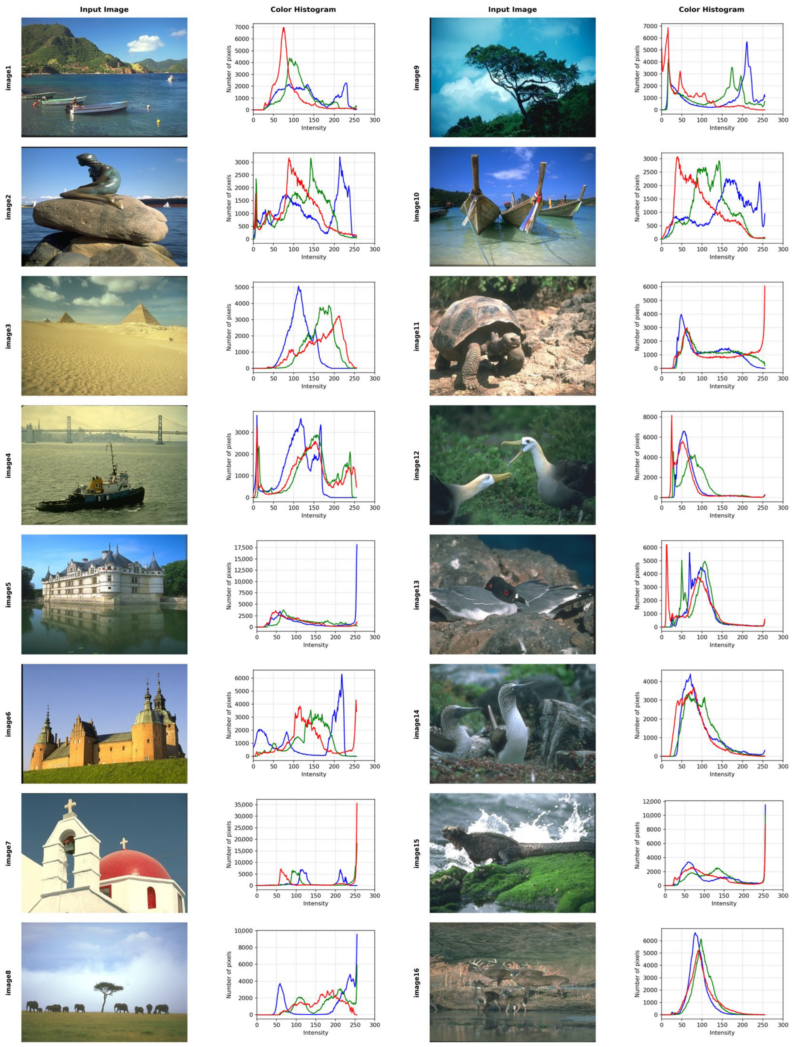
A higher total variance means the thresholds are better at separating different regions in the image. The optimization algorithm keeps improving the thresholds until the best possible value is found. By combining color information and edge information, the method produces more accurate and stable segmentation results. To find optimized threshold values, Brown Bear Optimization (BBOA) [19,20] is used. The proposed algorithm and other methods were experimented on ten natural color images, as illustrated in Figure 1. It also gives information regarding the histograms of all the input images considered; histograms of R, G, and B channels are depicted separately for all the input images.

4.1. Optimized Threshold: Selection Process for Otsu’s Method

Let the input color image considered for experimentation for image segmentation with the proposed methodand other state-of-the-art techniques be I R G B = { R ,   G ,   B } . For each color channel C { R ,   G ,   B } , the histogram h C ( i ) , i = 0, 1, …, N − 1, is computed, where L denotes the number of gray levels. In parallel, the RGB image is converted to grayscale and processed using the Sobel operator to obtain the edge image S, whose histogram h S ( i ) , represents the edge intensity distribution.
For multilevel thresholding with m thresholds, a threshold vector is defined as: T = {t1, t2, …, tm}, 0 < t1 < t2 < … < tm < L, which partitions each histogram into m + 1 classes.
For each channel C { R ,   G ,   B } , Otsu’s between-class variance is computed as:
σ C 2 T = ω c , k μ c , k μ c 2   ,   k = 0 , 1 , m
where ω c , k is the probability of class k, μ c , k is the mean intensity of class k, and μ c is the global mean intensity of channel c.
The total objective function is defined as the sum of variances from all four channels:
J ( T ) = σ R 2 T + σ G 2 T + σ B 2 T + σ S 2 T
the objective function: T* = arg max J(T)
During each iteration, the algorithm generates candidate threshold sets, evaluates J(T), and updates the thresholds based on the optimization strategy until convergence. The final optimized thresholds are applied to segment the image. By jointly maximizing inter-class separability across color and edge domains, the method achieves accurate and robust image segmentation. To express the efficiency of the proposed segmentation process, a comprehensive comparative study is conducted against well-established optimization techniques, including ABC, JA, MFO, PSO, and WOA.
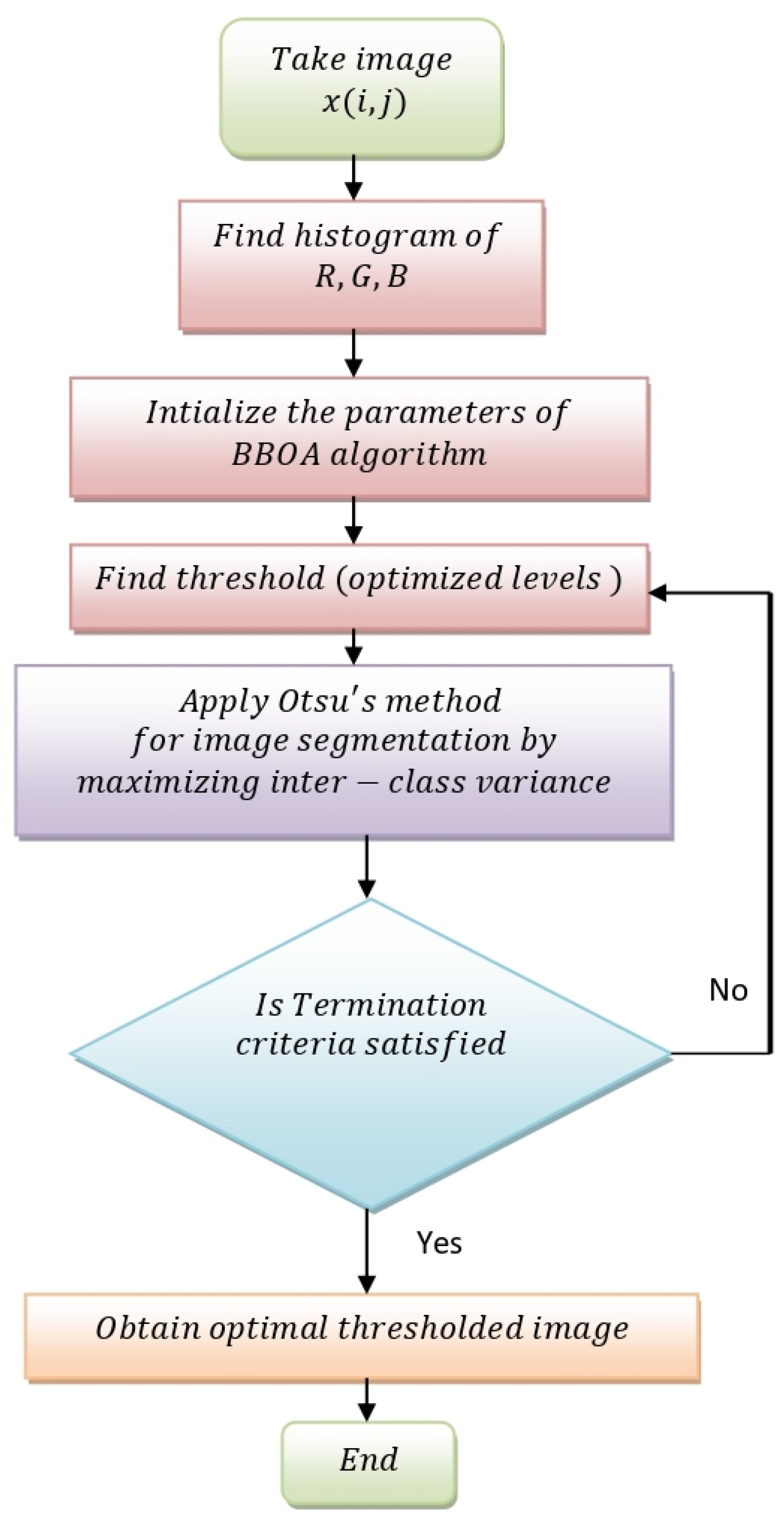
In the introduction, the range of multilevel thresholding methods for picture segmentation is discussed, along with the drawbacks of histogram-based methods, and the flow chart given in Figure 2. The suggested method used BBOA to discover optimal threshold values on a histogram by maximizing the inter-class variance in Otsu’s method, as provided in Equation (11). The experimental setup was executed several times until no significant further improvement in the fitness values was observed. The experiment was carried out on the system, Intel(R) Core(TM) i5, 8th generation, baseboard manufactured by LENOVA, Windows 11, and Python 3.9.11 codes developed for the required algorithms.
The flowchart illustrates an optimization-based image segmentation approach that combines Brown Bear Optimization Algorithm (BBOA) with Otsu’s thresholding method. Initially, the input color image x(i, j) is acquired, and its RGB components are separated. Histograms of the Red, Green, and Blue channels are computed to analyze the distribution of pixel intensities. Next, the parameters of the BBOA are initialized, and an initial population of candidate threshold sets is generated. BBOA then searches for optimal threshold levels by evolving these candidate solutions. For each candidate, Otsu’s method is applied to evaluate segmentation quality by maximizing the inter-class variance. A decision block checks whether the termination conditions, such as the number of iterations, are met. If the conditions are not met, the algorithm continues with the optimization process. When the conditions are met, the optimized threshold values are applied to the image for the purpose of obtaining the segmented output. This framework helps in obtaining improved results for image segmentation. The four variance values are summed up to get the total variance. Figure 2 illustrates the flowchart of the proposed image briefly. As the first step, each input image is taken for experimentation, and then the histograms of R, G, and Bcomponents of the images are computed. The design parameters required for BBOA are assigned, and resultantly, the optimized threshold values are computed by step-by-step maximizing the fitness function in the subsequent iterations. After determining the optimized threshold values, the images were segmented as per Otsu’s method, the effectiveness of the methods was computed in terms of comparative parameters as given in the Section 6.
Figure 2. Flow chart of proposed approach of BBOA_S.
Symmetry 18 00795 g002
The proposed method, although effective in improving segmentation quality, has certain limitations. The integration of RGB histograms, Sobel-based structural information, and BBOA optimization increases computational complexity, particularly for higher threshold levels and high-resolution images. The performance of the method further depends on the proper tuning of optimization parameters, and its effectiveness may be reduced in low-contrast images where edge information is weak.

4.2. Effect of the Sobel Filter on the Performance of the Proposed Method

The Sobel filter tends to highlight areas of high intensity change, thus making it effective in edge and object boundary detection. This means that the output from the Sobel operation tends to have high intensity values at edge pixels and low intensity values at uniform parts of the image. By calculating the histogram for the Sobel filtered image and using it in the objective function, our approach guarantees that the selected thresholds take both intensity value distribution and structural information into account.
The fusion method proves highly effective for improving the segmentation quality in many aspects. To begin with, it makes sure that edges remain intact after the application of the threshold. It is due to the fact that it prevents over-smoothing issues that could happen during a histogram-based process. The combination guarantees that details remain untouched while the algorithm performs the task. Hence, it means that the structure of the image becomes closer to the original one. Such an improvement can be easily seen on SSIM and FSIM. Namely, SSIM focuses on luminance, contrast, and structural similarity. Therefore, the presence of edges obtained by applying the Sobel method allows for increasing the score of SSIM.
Otsu’s multilevel thresholding criterion maximizes between-class variance, a functional that is invariant to permutations of color channels in RGB space. Formally, the between-class variance objective Σ wₖ(μₖ − μ)2 remains unchanged under any symmetric relabeling of intensity levels, confirming that the method exhibits class-label symmetry. The Sobel operator computes gradient magnitude as G = √(Gx2 + Gy2), which is rotationally symmetric—the edge response is direction-agnostic and consistent under 90° rotations of local image structure. This property ensures that the Sobel-derived histogram captures structurally equivalent edge information regardless of object orientation, making it a robust feature for integration with RGB histograms. The fusion of RGB histograms with Sobel edge histograms inherits both symmetries: the channel invariance of Otsu’s objective and the rotational invariance of Sobel gradients. Together, they ensure that the fused feature space is symmetric under color permutation and spatial rotation, which directly stabilizes the Brown Bear Optimization (BBO) objective function landscape—reducing asymmetric local optima and improving convergence reliability.

5. Experimental Setup

The proposed method, along with other image segmentation techniques, has been evaluated on 100 images from the Berkeley segmentation data set BSDS500), out of which 16 representative segmented results are presented in the paper. The complete set of segmented images and detailed statistical analysis is provided as Supplementary Material and can be accessed through the Google Drive link. All experiments were conducted on a system with an Intel(R) Core(TM) i5-8250U CPU @ 1.60 GHz (up to 1.80 GHz), 8 GB RAM, and a 64-bit operating system based on an x64 architecture. Python is used to implement the algorithms. The additional data for 100 images, like input and outputimages, all parameter values for 100 images are given on the link https://drive.google.com/drive/folders/12is0nz2KI87VPpZHdyMHNlIJbzAH2Imt?usp=drive_link (accessed on 27 April 2026).
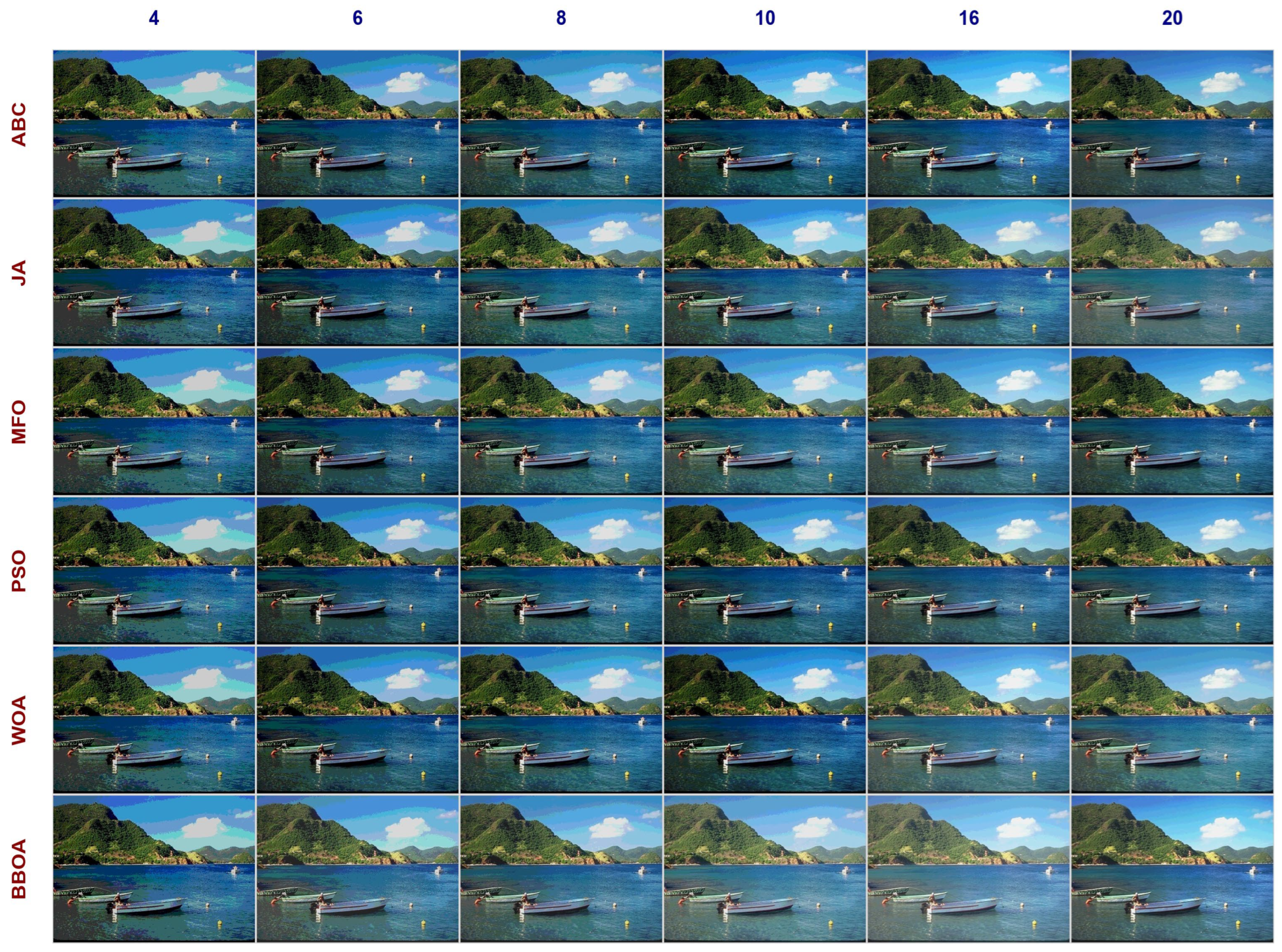
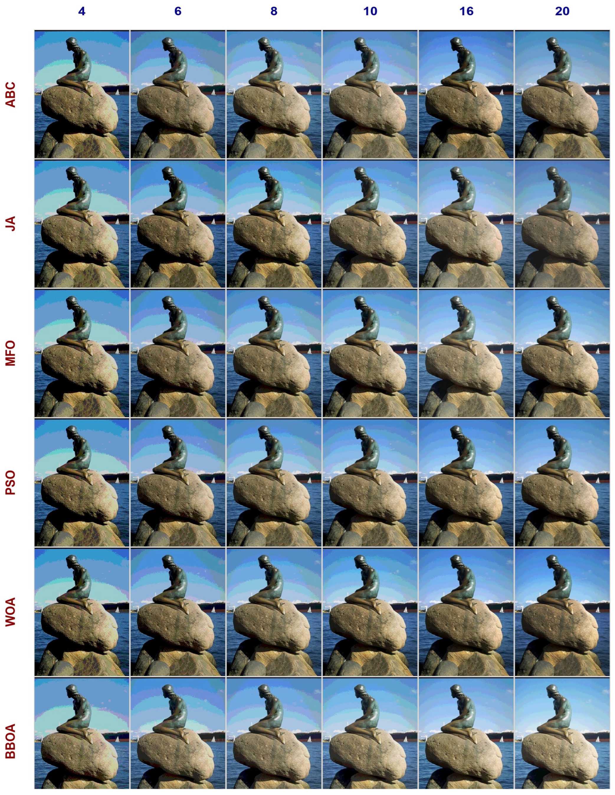
All test images were evaluated at multiple threshold levels, specifically 4, 6, 8, 10, 16, and 20. In the experimental setup, the parameter settings for all optimization algorithms are clearly defined to ensure fair comparison and reproducibility. For WOA, the parameter ‘a’ is linearly decreased in the range [0, 2], ‘b’ is set to 1 to define the logarithmic spiral shape, and ‘l’ is a random value in the range [−1, 1]. For PSO, the cognitive and social coefficients C1 and C2 are both set to 2, while the inertia weight varies between W M A X = 0.9 and W M I N = 0.2. In the case of ABC, the ‘limit’ parameter, representing the maximum trial count, is fixed at 25. For MFO, the parameter ‘b’ is set to 1 to control the spiral path shape, and ‘θ’ is a random value within [−1,1] to update the moth position. Additionally, for all methods, the population size is uniformly set to 30, and the number of iterations is fixed at 400 to maintain consistency across experiments.

5.1. Computation of Weight for R, G, B, and Sobel Channel Based on Entropy

Step 1: Construct the Decision Matrix
Let the segmented image produce classes (threshold levels) foreachofthefourchannels {R, G, B, S}. Construct the decision matrix using between-class variance for each class and channel:
X = [ X i j ]   w h e r e   i = 1 , 2 , k c l a s s e s   a n d   j = R , G , B , S ( c h a n n e l s )
Eachentry X i j represents the between-class variance of class i in channel j.
Step 2: NormalizetheDecisionMatrix
Normalize each entry to obtain probability-like values:
p i j = x i j i = 1 k x i j
This ensures each column sums to 1, making values comparable across channels despite dimensional differences between RGB intensity and Sobel gradient features.
Step 3: Compute Entropy for Each Channel
For each channel j, compute the Shannon entropy:
H j = 1 ln k i = 1 k p i j . l n ( p i j )
where
k = number of segmentation classes (thresholding levels).
The factor 1 l n ( k ) normalizes entropy to the range [0, 1].
If p i j = 0 , define p i j . ln p i j = 0 to avoid undefined values.
Interpretation:
High H j → channel j has uniform variance across classes’ → less discriminative.
Low H j → channel j has concentrated variance → more discriminative.
Step 4: Compute Degree of Divergence:
The degree of divergence (information utility) for each channel
d j = 1 H j
A higher d j means channel j provides more unique and useful information for segmentation.
Step 5: Compute Entropy Weights
Normalize the divergence values to get final weights:
w j = d j j = 1 4 d j = 1 H j j = 1 4 ( 1 H j )
This guarantees:
W R + W G + W B + W S = 1
By using the above process, the weights for four channels will be calculated
No manual tuning required, and weights are data-driven
Step 6: Final Revised Objective Function
Substituting entropy weights into the objective function:
F = W R σ R 2 + W G σ G 2 + W B σ B 2 + W S σ S 2

5.2. Computation of Dice Similarity Coefficient (DSC)

The Dice Similarity Coefficient (DSC) is a statistical measure used to evaluate the similarity between two sets. It is widely used in fields like image processing, natural language processing, and especially medical image segmentation. The Dice coefficient measures how much two sets overlap relative to their total size, with its value ranging from 0 to 1.
D i c e   C o e f f i c i e n t = 2 | A B | A + | B |
where
A = predicted set (e.g., segmented image);
B = ground truth set;
A ∩ B = number of common elements (overlap).
Dice in Image Segmentation: In image processing, the formula is often written as:
D i c e   C o e f f i c i e n t = 2 A r e a   o f   O v e r l a p T o t a l   p i x e l s   i n   b o t h   s e g m e n t a t i o n s

5.3. Computation of the Wilcoxon Signed-Rank Test

The Wilcoxon Signed-Rank Test is a non-parametric statistical test used to compare two related samples.
Procedure
Step 1: Collect Data: Take thevalues of (PSNR) for two different methods, for example, Method A (PSNR), and Method B (PSNR).
Step 2: Compute Differences
D = A B
Step 3: Remove Zero Differences:Ignore rows where = 0.
Step 4: Rank Absolute Differences: Take | D | , Assign ranks (smallest = 1).
Step 5: Assign Signs:
If D > 0 P o s i t i v e   R a n k ;
If D < 0 N e g a t i v e   R a n k .
Step 6: Calculate Rank Sums
W + = S u m   o f   p o s i t i v e   R a n k s
W = S u m   o f   n e g a t i v e   R a n k s
Step 7: Test Statistic: W = min W + , W .
Step 8: Decision Rule: Compare p-value with significance level (0.05):
If p < 0.5 R e j e c t   H 0   ( S i g n i f i c a n t   D i f f e r e n c e ) ;
If p 0.5 A c c e p t   H 0 n o   S i g n i f i c a n t   D i f f e r e n c e .
In this paper, the reslts are presenetd in Table 1, Table 2, Table 3, Table 4, Table 5, Table 6 and Table 7, and the Wilcoxon Signed-Rank Test is conducted on 100 images, and the proposed method is compared with all other methods; its results are depicted in Table 8.

6. Results and Discussions

The segmented images with various optimization techniques, along with Otsu’s method, and segmented images with the proposed method are given in images 3 to 13, the comparative parameters given in the Table 1, Table 2, Table 3, Table 4, Table 5, Table 6, Table 7, Table 8 and Table 9, and Figure 3, Figure 4, Figure 5, Figure 6, Figure 7, Figure 8, Figure 9, Figure 10, Figure 11, Figure 12, Figure 13, Figure 14, Figure 15, Figure 16 and Figure 17 illustrate the effectiveness of the proposed method in terms of metrics in graphical form. As illustrated in Figure 1, a total of sixteen images are taken into consideration for testing on Python.
The performance of the proposed approach for segmentation BBOA_S, based on the RGB–Sobel multilevel thresholding approach, is evaluated using ten benchmark color images and compared with five state-of-the-art optimization algorithms, including ABC, JA, MFO, PSO, and WOA. Quantitative assessment is done using widely used image quality and segmentation comparative metrics, namely PSNR, MSE, SSIM, and FSIM, whose average values are summarized in the experimental results given in the tables. All the algorithms used for comparing the effectiveness of the proposed method were executed until there was no change in the fitness function.
Table 1. Comparison of PSNR of segmentation with Otsu’s method based on optimization techniques ABC, JA, MFO, PSO, and WOA with Proposed Model BBOA_S. Note: The bold number indiacted the best value.
ImageThABCJAMFOPSOWOABBOA_S
image 1418.102317.684917.927217.927217.912119.2709
617.463017.001617.239417.239417.419725.5453
819.147820.650120.402619.693519.518226.6486
1017.210721.536922.112218.535617.156022.7336
1619.576223.871524.430022.546627.193019.5861
2019.892329.324120.642223.046726.264325.8444
image 2421.158121.646320.809320.809320.876423.3793
622.822120.604822.553522.841622.597526.8484
827.474323.975726.266626.266627.225928.9777
1029.925629.744028.251727.807925.263126.3796
1623.187727.210026.880426.117526.813425.2709
2026.184625.019331.329028.911923.737720.8034
image 3413.842213.399413.168813.168813.051215.5854
615.499514.079514.782716.034915.025520.0748
813.864014.889615.120015.208416.689723.0441
1018.554815.831515.249316.099521.278825.4524
1615.050418.042618.247220.228719.035925.4382
2024.815815.650221.206217.266917.054728.9289
image 4419.419219.924619.649519.649519.649520.4199
619.164818.842819.569619.569619.000824.7190
819.882621.893222.896822.842322.264325.1782
1018.326021.984923.227422.587821.964529.4729
1625.449224.049227.017221.813628.299727.4408
2022.058327.798222.218819.697027.254426.8987
image 5416.224315.520916.396616.406616.362819.1593
618.410319.489118.184518.184518.293024.1073
819.963120.739919.977819.836419.729425.5850
1019.914917.496819.288821.139422.885924.0438
1627.714019.486725.591823.083121.886620.1768
2027.336224.144722.006724.193029.054232.4294
image 6416.973517.460616.997616.997616.959717.8519
621.742720.189721.777221.777223.771425.9393
822.765621.619227.758323.039222.390727.8500
1025.296723.966927.502725.687225.079027.3013
1629.210224.643430.737327.613926.340122.5226
2025.906428.250029.994227.275921.819726.7869
image 7413.751513.973113.770813.770813.770816.5110
616.027116.755616.020716.020715.474120.2751
818.505417.700518.365918.296914.658319.8400
1020.103617.545120.131820.987420.163224.7539
1619.733721.137121.257220.847927.350627.0932
2018.156618.180618.399521.384318.665724.4756
image 8412.131812.693712.273612.273612.273612.7585
613.880014.075713.792013.904213.731814.5715
814.440413.937613.356013.436315.133317.9497
1015.363313.005914.824215.136115.104418.6039
1616.403017.667217.564718.168015.387419.0622
2016.694814.606914.941618.224218.532924.1860
image 9422.477722.587822.320222.222322.222322.8134
622.422622.024021.647121.647121.601522.4413
823.723719.699522.262421.709920.550526.7291
1025.679427.059825.353326.914227.935928.6872
1623.037027.517728.900428.882724.696627.6379
2029.920129.175031.477829.875127.382627.4231
image 10416.947917.241817.034717.034717.073717.9431
618.842119.813218.544418.544418.721125.6907
820.192222.618321.002320.787519.059228.5032
1022.819318.430422.066523.700327.121528.8034
1628.178923.639326.375925.389326.312429.9059
2023.117422.469927.139025.866923.926225.8385
Average 20.534620.353621.103920.769520.899523.8365
Table 2. Comparison of SSIM ofsegmented with Otsu’s method based on optimization technique ABC, JA, MFO, PSO, and WOA with Proposed Model BBOA_S with N = 4, 6, 8, 10, 16 and 20.
ImageThABCJAMFOPSOWOABBOA
image 140.89250.88490.88720.88720.88700.9225
60.87590.85970.87080.87080.87470.9884
80.90970.93560.93120.91880.91670.9894
100.85630.95200.95420.89820.86160.9862
160.92800.97680.97680.96140.99340.9722
200.93200.99440.93790.96370.98860.9947
image 240.94800.95050.94250.94250.94400.9739
60.97420.94190.96370.96640.96250.9911
80.98940.97180.98450.98450.98840.9951
100.99520.99520.99030.98900.98160.9936
160.96950.99400.99390.98380.98660.9930
200.99050.99160.99480.98870.98060.9829
image 340.82980.80990.80600.80600.80300.8784
60.87560.85690.86190.89250.87170.9644
80.83120.87580.87700.87900.90700.9800
100.94040.89550.88260.89640.97040.9906
160.86870.93600.94800.95810.95480.9957
200.98610.91520.96700.92450.92970.9978
image 440.95330.95940.95520.95520.95520.9649
60.95390.95130.95550.95550.94950.9857
80.95420.97610.97520.97470.97150.9865
100.94320.96930.97570.97320.97140.9942
160.98610.98560.98940.96750.99070.9946
200.98110.99160.97630.95610.98830.9954
image 540.80890.78070.81720.81730.81620.9162
60.89300.91230.88530.88530.89130.9875
80.92440.92480.91150.90920.91300.9908
100.89650.88080.89960.92950.95090.9901
160.98410.93830.97270.95030.94180.9679
200.98630.98130.95470.96190.99260.9975
image 640.91340.91730.91150.91150.91130.9280
60.97030.94400.96670.96670.97780.9926
80.97410.96220.99370.97300.97230.9963
100.99050.98070.99210.98860.98330.9959
160.99350.99250.99770.99450.98920.9904
200.99440.99450.99550.98710.97320.9970
image 740.81290.82420.81460.81460.81460.9548
60.87290.88850.87270.87270.87350.9782
80.94670.93920.94800.94750.82620.9619
100.96250.92520.95650.96210.95460.9940
160.95540.98350.95340.95060.99380.9924
200.93300.93160.92090.96140.91880.9825
image 840.79970.81310.80680.80680.80680.8307
60.85270.85530.85320.85450.85110.8805
80.86860.85800.84230.84390.87630.9578
100.89920.82540.87860.88550.90700.9616
160.91470.95310.95050.93290.87070.9566
200.92520.93870.89870.92830.96130.9929
image 940.95900.96180.95860.95630.95630.9653
60.96940.95800.96030.96030.95970.9743
80.95980.93880.96410.95980.94210.9918
100.99220.99370.97630.98680.99520.9947
160.95800.99320.99700.99720.96580.9925
200.99560.99160.99560.99640.99570.9819
image 1040.87160.86850.86980.86980.87080.8955
60.91010.92260.90070.90070.90500.9851
80.91200.94830.93650.93570.91790.9931
100.97270.91380.94820.96290.98300.9954
160.99490.96510.98170.97890.97430.9975
200.96700.95970.98780.97810.96520.9916
Average 0.93170.93220.93450.93350.93380.9744
Table 3. Comparison of average PSNR of segmented with Otsu’s method based on optimization technique ABC, JA, MFO, PSO, and WOA with Proposed Model BBOA_S with N = 4, 6, 8, 10, 16 and 20.
ImageABCJAMFOPSOWOAPROPOSED-BBOA_S
image 118.565421.678220.458919.831520.910623.2715
image 225.125424.726.015125.459124.41925.2765
image 316.937815.315516.295716.334517.022623.0873
image 420.716722.415522.429921.026623.072225.6882
image 521.593819.479720.24120.473821.368624.2503
image 623.649222.688325.794523.731922.726824.7087
image 717.71317.548717.99118.551318.347122.1581
image 814.818914.331214.458715.190415.027317.8553
image 924.543424.677325.326825.208524.064925.9553
image 1021.682920.702222.027121.887222.035726.1141
image 1118.213819.551817.410318.03220.007325.6012
image 1222.206821.72422.814822.04223.757820.7747
image 1320.475823.635222.944322.916323.199724.2743
image 1420.144620.568120.466120.46720.475121.602
image 1520.322719.64920.115120.172719.819623.871
image 1619.713820.008319.691620.009620.983519.3699
Average20.401520.542120.905120.708421.077423.3661
Table 4. Comparison of average MSE of segmented with Otsu’s method based on optimization technique ABC, JA, MFO, PSO, and WOA with Proposed Model BBOA_S with N = 4, 6, 8, 10, 16 and 20.
ImageABCJAMFOPSOWOABBOA_S
image 1930.5827627.3326677.2785761.4689747.5854387.0383
image 2248.1134278.0738222.1674230.2583269.3487233.0946
image 31723.7412018.7311784.0781691.3861539.327535.5166
image 4624.296451.0898430.8746540.7828423.6016221.7498
image 5672.9781873.8411747.8536702.9724665.7344356.5244
image 6420.2638469.7618345.7511410.4835456.3273326.6203
image 71267.0141285.8231226.5851140.4621404.549552.2802
image 82292.0352547.5752489.1832234.882233.2891451.533
image 9263.4775297.4927255.3262259.4666309.3735194.4388
image 10589.9949640.7751565.3308562.0735582.9153272.1603
image 111229.8131115.6471290.2921172.478974.456263.7035
image 12418.3683486.2095376.6451421.4045346.5139571.2434
image 13717.2836320.1103352.0872355.4117339.7093318.7525
image 14693.3778762.1774607.5395619.9586660.2502517.4034
image 15864.3101945.8161826.7172770.2505835.4633374.1697
image 16745.1078810.7381808.931713.6979615.9466821.6369
Average856.2974870.6996812.915786.7146775.2745462.3666
Table 5. Comparison of average SSIM of segmented with Otsu’s method based on optimization technique ABC, JA, MFO, PSO, and WOA with Proposed Model BBOA_S with N = 4, 6, 8, 10, 16 and 20.
ImageABCJAMFOPSOWOABBOA_S
image 10.89910.93390.92630.91670.92030.9756
image 20.97780.97420.97830.97580.97390.9883
image 30.88860.88150.89040.89270.90610.9678
image 40.96190.97220.97120.96370.97110.9869
image 50.91560.9030.90680.90890.91760.975
image 60.97270.96520.97620.97020.96780.9834
image 70.91390.91540.9110.91820.89690.9773
image 80.87670.8740.87170.87530.87890.93
image 90.97230.97290.97530.97610.96910.9834
image 100.9380.92970.93750.93770.9360.9764
image 110.8720.8760.870.86840.89590.9787
image 120.92310.93910.93960.93350.9380.9541
image 130.970.9710.96380.9630.96230.9675
image 140.90410.92780.96320.90660.91760.9242
image 150.90450.90520.90830.91180.91180.9737
image 160.93430.92380.92390.9350.9480.9698
Average0.92650.92910.93210.92830.9320.9695
Table 6. Comparison of average FSIM of segmented with Otsu’s method based on optimization technique ABC, JA, MFO, PSO, and WOA with Proposed Model BBOA_S with N = 4, 6, 8, 10, 16 and 20.
ImageABCJAMFOPSOWOABBOA_S
image 10.73780.73340.74580.74650.73900.7339
image 20.72510.72130.73350.73290.72990.7265
image 30.68100.66920.69370.69540.68750.6679
image 40.72960.72430.73730.73250.73430.7372
image 50.70970.70340.72200.72170.71420.7062
image 60.68300.67830.69360.69020.68310.6943
image 70.68260.68230.68550.68460.68410.6708
image 80.56850.55580.57290.57900.56970.5587
image 90.70780.71050.72050.72020.71210.7233
image 100.68430.67990.69750.69680.69290.6884
Table 7. Comparison of average Dice Similarity Coefficient (DSC) of segmented with Otsu’s method based on optimization technique ABC, JA, MFO, PSO, and WOA with Proposed Model BBOA_S with N = 4, 6, 8, 10, 16 and 20.
ImageABCJAMFOPSOWOABBOA_S
image 10.89910.93390.92630.91670.92030.9756
image 20.97780.97420.97830.97580.97390.9883
image 30.88860.88150.89040.89270.90610.9678
image 40.96190.97220.97120.96370.97110.9869
image 50.91560.9030.90680.90890.91760.975
image 60.97270.96520.97620.97020.96780.9834
image 70.91390.91540.9110.91820.89690.9773
image 80.87670.8740.87170.87530.87890.93
image 90.97230.97290.97530.97610.96910.9834
image 100.9380.92970.93750.93770.9360.9764
image 110.8720.8760.870.86840.89590.9787
image 120.92310.93910.93960.93350.9380.9541
image 130.970.9710.96380.9630.96230.9675
image 140.90410.92780.96320.90660.91760.9242
image 150.90450.90520.90830.91180.91180.9737
image 160.93430.92380.92390.9350.9480.9698
Average0.92650.92910.93210.92830.9320.9695
Table 8. Comparison of WILCOXON of segmented with Otsu’s method based on optimization technique ABC, JA, MFO, PSO, and WOA with Proposed Model BBOA_S by considering 100 images.
Method 1Method 2Metric UsedMean of Method 1Mean of Method 2Wilcoxon_
Statistic
p-ValueSignificantBetter Method
BBOA_SABCPSNR23.244221.577547,6481.44 × 10−23YesBBOA_S
BBOA_SABCMSE464.3813637.778750,6741.5 × 10−20YesBBOA_S
BBOA_SABCSSIM0.97160.94727,8531.08 × 10−48YesBBOA_S
BBOA_SABCDSC0.95950.93520,5972.96 × 10−60YesBBOA_S
BBOA_SJAPSNR23.244221.636650,3407.14 × 10−21YesBBOA_S
BBOA_SJAMSE464.3813663.57449,7021.7 × 10−21YesBBOA_S
BBOA_SJASSIM0.97160.947430,7451.94 × 10−44YesBBOA_S
BBOA_SJADSC0.95950.94139,3505.83 × 10−33YesBBOA_S
BBOA_SMFOPSNR23.244221.655446,921.52.53 × 10−24YesBBOA_S
BBOA_SMFOMSE464.3813640.63949,644.51.49 × 10−21YesBBOA_S
BBOA_SMFOSSIM0.97160.947826,682.51.79 × 10−50YesBBOA_S
BBOA_SMFODSC0.95950.935616,426.51.8 × 10−67YesBBOA_S
BBOA_SPSOPSNR23.244221.906752,4426.88 × 10−19YesBBOA_S
BBOA_SPSOMSE464.3813592.688156,5042.36 × 10−15YesBBOA_S
BBOA_SPSOSSIM0.97160.948526,5391.08 × 10−50YesBBOA_S
BBOA_SPSODSC0.95950.93226461.52.11 × 10−86YesBBOA_S
BBOA_SWOAPSNR23.244221.677249,411.58.79 × 10−22YesBBOA_S
BBOA_SWOAMSE464.3813639.968252,518.58.09 × 10−19YesBBOA_S
BBOA_SWOASSIM0.97160.949230,782.52.2 × 10−44YesBBOA_S
BBOA_SWOADSC0.95950.936319,166.51.1 × 10−62YesBBOA_S

6.1. Importance of Evaluation Metrics

6.1.1. Peak Signal-to-Noise Ratio (PSNR)

PSNR is a widely used metric to evaluate the overall fidelity of the segmented or enhanced image with respect to the original image. It quantifies how much noise or distortion is introduced during the segmentation process.
In the proposed method, higher PSNR values indicate that the optimized multilevel thresholds preserve the original image information more effectively. Since the approach jointly optimizes RGB and edge-based histograms, PSNR validates the global accuracy and stability of the segmentation outcome.

6.1.2. Mean Squared Error (MSE)

The mean value of the squared differences between the input original image and the resultant segmented image is given asMSE. A low MSE value indicates minimal reconstruction error and accurate segmentation boundaries.
In the proposed framework, the low MSE value shows the effectiveness of the proposed algorithm in choosing the optimal thresholds, which ensures the accurate assignment of pixel intensity values while minimizing the loss of information.

6.1.3. Structural Similarity Index (SSIM)

SSIM measures the perceptual image quality based on luminance, contrast, and structural consistency rather than pixel-wise differences. In the presented work, SSIM plays a significant role in ensuring that the suggested method maintains the structural and textural information, especially the edges and boundaries of objects that are enhanced by the Sobel operator. High SSIM ensures that the segmented images are meaningful and consistent.

6.1.4. Feature Similarity Index (FSIM)

FSIM is based on the evaluation of the quality of the images, which depends on the preservation of low-level features such as phase congruency and gradient magnitude, which are directly associated with the perception of the images by the human eye. The importance of FSIM in this study is that it is used to validate that the segmentation process is preserving the essential features of the images, especially in areas where the texture is fine.

6.2. Overall Significance of Metric Selection

The combined use of PSNR and MSE measures the numerical accuracy, while SSIM and FSIM measure the perceptual and feature-level quality measures, and the effectiveness of image segmentation. These measures ensure that the proposed RGB–Sobel-based optimization technique provides perfect, perceptually consistent, and structurally robust image segmentation results.
Using 10 benchmark color images, the effectiveness of the suggested BBOA-based RGB–Sobel multilevel thresholding technique is assessed and contrasted with five cutting-edge optimization algorithms: ABC, JA, MFO, PSO, and WOA. Widely recognized image quality and segmentation metrics, including as PSNR, MSE, SSIM, and FSIM, are used for quantitative evaluation; the experimental findings summarize the average values of these metrics.
The segmented image’s fidelity in relation to the original image is measured by PSNR. Better image information preservation is indicated by higher PSNR values. According to the results, the suggested approach routinely outperforms rival algorithms in terms of PSNR values for the majority of test photos. Specifically, the suggested approach shows a noticeable increase for images like images 1 to 16, with PSNR gains exceeding 3–6 dB in several situations. This result demonstrates that class separability is effectively improved and distortion during multilevel thresholding is reduced when RGB channel histograms and Sobel edge information are jointly optimized.
Pixel-wise reconstruction error is described by the value of MSE. It has an inverse relationship with PSNR. As presented in the findings, for the majority of the test images, particularly images 1 to 5 and images 7 and 10, the suggested BBOA_S method achieves the minimum values of MSE. For example, the values of MSE for image 3 are almost tripled compared to the conventional optimization methods. Such a reduction in the values of MSE indicates the efficiency of the suggested objective function based on between-class variance, which considers the characteristics of color and edges. As a result, the precision of the image segmentation outcome is better, as well as the selection of the threshold.
SSIM considers structural information, contrast, and brightness when assessing the quality of the perceptual image. As presented in the findings, for the majority of the test images, the suggested approach achieves high values of SSIM, which often exceed 0.97. The suggested method significantly outperforms the ABC, JA, MFO, PSO, and WOA methods, particularly for the test images with complex structures, such as image 1, image 3, image 7, and image 8.
FSIM is based on the preservation of low-level features, including phase congruency and gradient magnitude. The results showed that the FSIM values of the proposed method were comparable to, or slightly lower than, the best-performing existing methods on some images. This behavior of the proposed method suggests that, although it focuses on global class separation and structural consistency, it still achieves comparable feature-level similarity, especially for some images, such as image 4, image 6, and image 9. The improved PSNR, MSE, and SSIM results verify that the quality of the segmentation is more stable and meaningful.
Thus, to briefly conclude on the effectiveness of the proposed RGB–Sobel integrated Otsu optimization framework based on BBOA optimization, it is clearly a better option for improved image quality, handling of noisy data, and maintaining structure compared to other optimization techniques for thresholding functions. The use of edge information along with color information is quite reliable for thresholding functions, especially for images with varying illumination conditions or those with complex texture features. Therefore, this proposed method is a better option compared to the previously proposed top-tier techniques for color image segmentation.
This section provides an exhaustive insight into the illustration of the BBOA_S-based multilevel image segmentation framework using quantitative results presented in the form of Table 1, Table 2, Table 3, Table 4, Table 5, Table 6, Table 7, Table 8 and Table 9. For the comparison, the proposed algorithm is compared with the prominent optimization techniques such as Artificial Bee Colony, Jaya Algorithm (JA), Moth Flame Optimization (MFO), Particle Swarm Optimization (PSO), and Whale Optimization Algorithm (WOA) using ten benchmark images with different threshold levels, N = 4, 6, 8, 10, 16, 20.
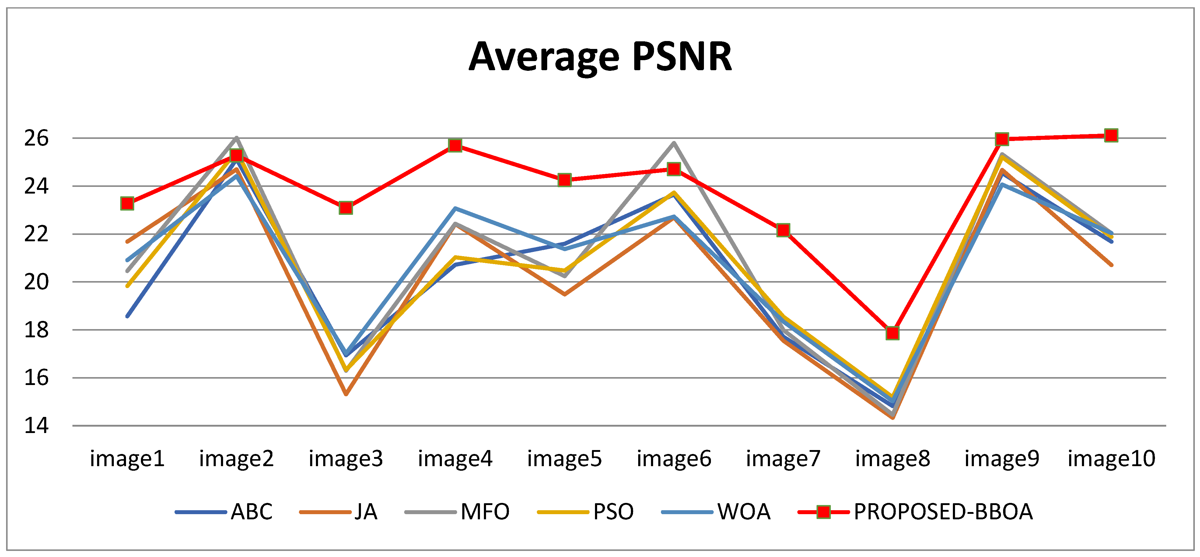
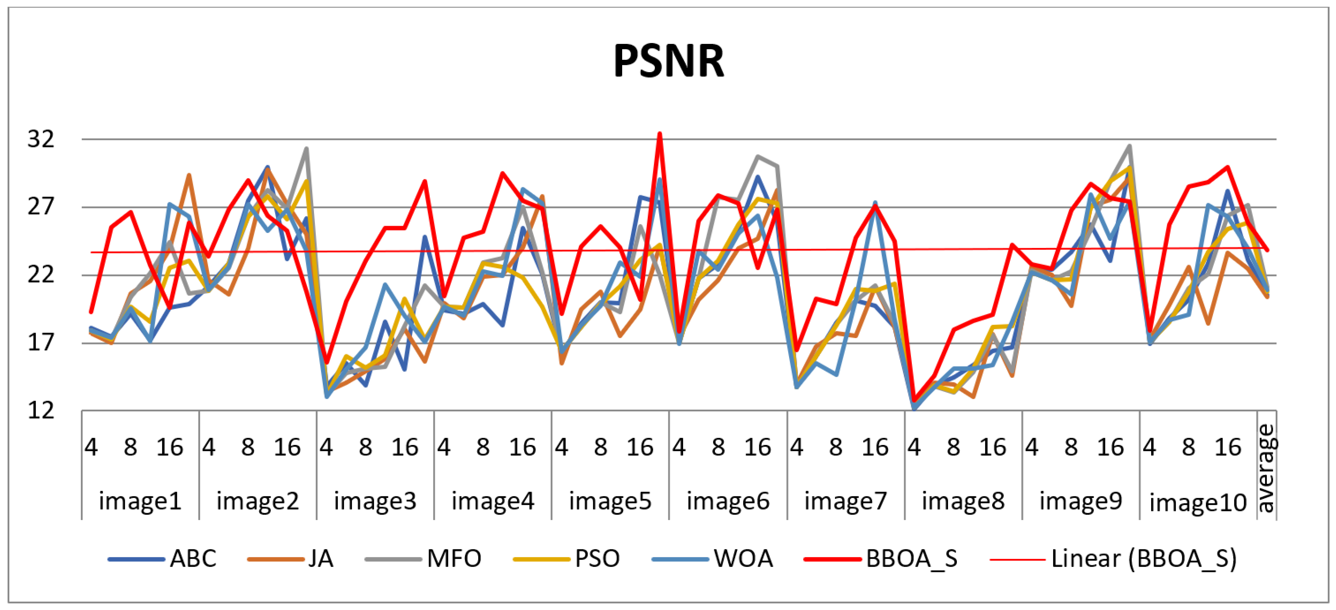
The PSNR is a prominent metric to evaluate the quality of image segmentation, where a higher PSNR indicates better reconstruction with minimal distortion. As depicted in Table 3, the proposed BBOA_S algorithm consistently achieves superior PSNR values compared to other optimization techniques such as ABC, JA, MFO, PSO, and WOA across most of the test images. For instance, in image 1, the proposed method attains a PSNR of 23.27, which is significantly higher than ABC (18.56), PSO (19.83), and WOA (20.91). Similarly, for image 10, the proposed method achieves a PSNR of 26.11, outperforming MFO (22.03) and WOA (22.04). Although in a few cases, such as image 12 and image 16, the performance is slightly lower, the overall trend clearly indicates the robustness of the proposed method. The average PSNR values further validate this observation, where ABC, JA, MFO, PSO, WOA, and the proposed BBOA_S achieve 20.40, 20.54, 20.91, 20.71, 21.07, and 23.37, respectively. This demonstrates that the proposed BBOA_S method provides a noticeable improvement in segmentation quality over existing techniques. Additionally, Figure 15 illustrates the PSNR comparison of all segmented images, where the proposed method (shown in red color) consistently outperforms others, and Figure 16 presents the average PSNR values across different threshold levels, reinforcing the effectiveness and stability of the proposed approach.
Better segmentation accuracy is indicated by lower Mean Squared Error (MSE) values, which quantify the reconstruction error between the original and segmented images. As shown in Table 4, the proposed BBOA_S algorithm achieves the lowest MSE values for the majority of the test images compared to ABC, JA, MFO, PSO, and WOA. For instance, in image 9, BBOA_S records a minimum MSE of 194.44, which is significantly lower than ABC (263.48), JA (297.49), and WOA (309.37). Similarly, for image 1, the proposed method reduces the MSE to 387.04, whereas ABC and JA exhibit much higher errors of 930.58 and 627.33, respectively. In image 4 and image 11, BBOA_S also demonstrates substantial error reduction with values of 221.75 and 263.70, outperforming all other methods. Although in a few cases such as image 12 and image 16 the MSE is comparatively higher, the overall performance trend clearly favors the proposed approach. The average MSE values further validate this observation, where ABC, JA, MFO, PSO, WOA, and BBOA_S achieve 856.30, 870.70, 812.92, 786.71, 775.27, and 462.37, respectively, indicating a significant reduction in error by the proposed method. These results confirm that BBOA_S effectively minimizes intra-class variance and preserves important image details, leading to superior segmentation performance.
The SSIM evaluates how effectively contrast, brightness, and structural information are preserved in the segmented image compared to the original image. It is an important metric, especially for the segmentation of natural color images. As shown in Table 5, the proposed BBOA_S method consistently achieves higher SSIM values across most benchmark images.
For example, in image 1, BBOA_S attains an SSIM of 0.9756, outperforming ABC (0.8991) and PSO (0.9167). Similarly, for image 3, the proposed method achieves 0.9678, whereas other methods produce values below 0.91.
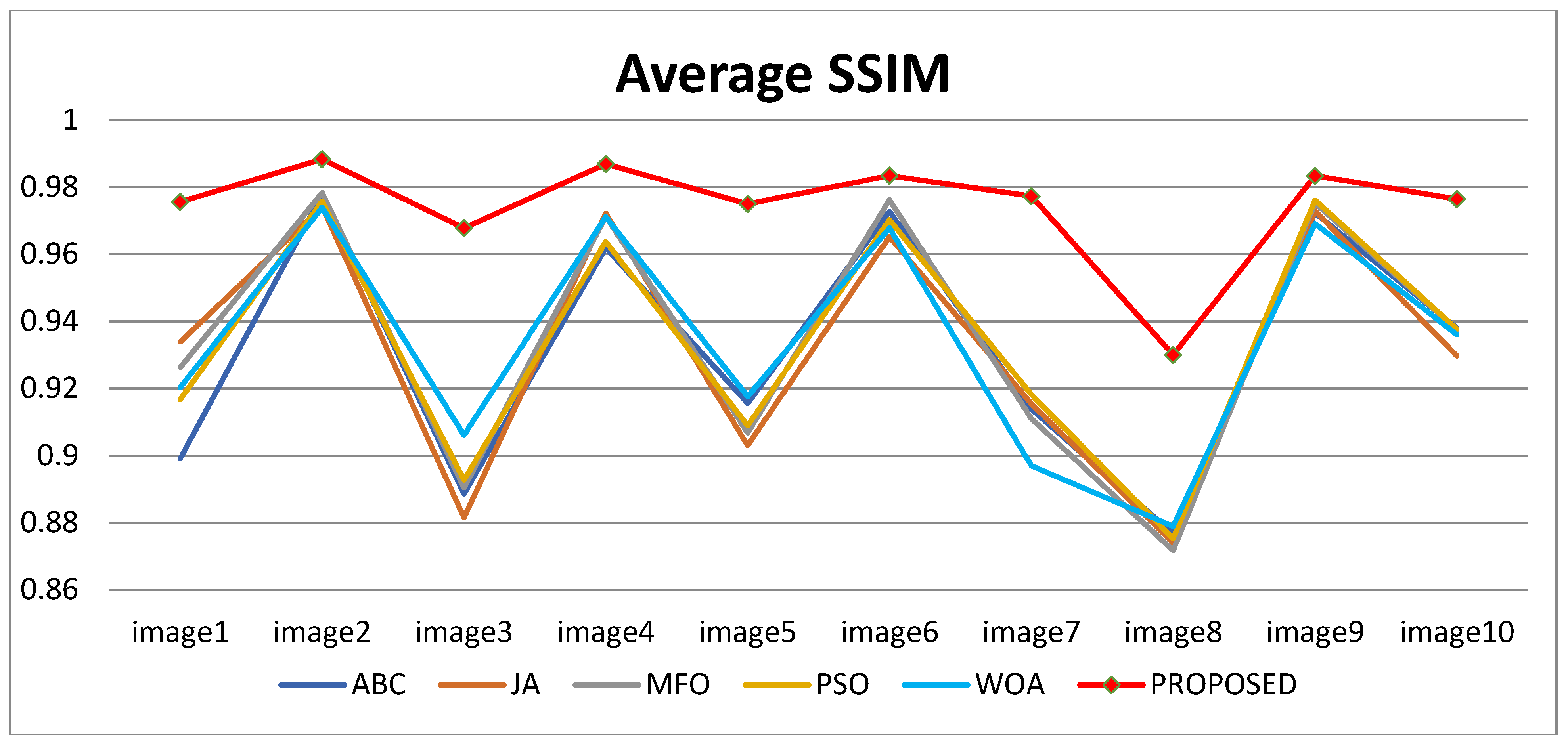
In image 11, BBOA_S reaches 0.9787, which is significantly higher than WOA (0.8959) and other techniques. For image10, the proposed method also shows improvement with an SSIM of 0.9764 compared to others around 0.93. Although in some cases, like image 14, the improvement is moderate, the overall performance remains superior. The average SSIM values clearly validate this trend. ABC, JA, MFO, PSO, WOA, and BBOA_S achieve 0.9265, 0.9291, 0.9321, 0.9283, 0.9320, and 0.9695, respectively. This indicates better structural similarity and visual quality for the proposed method. Figure 17 further illustrates that BBOA_S (shown in red) consistently outperforms other methods.
The preservation of important picture features is the main goal of the Feature Similarity Index (FSIM). Table 2 shows detailed FSIM values at various thresholds, while Table 6 displays average FSIM values. Table 2 shows that BBOA_S regularly obtains very high FSIM values, frequently above 0.99. For example, image 3 at N = 20 and image 10 at N = 10 have FSIM values of 0.9978 and 0.9954, respectively.
The Dice Similarity Coefficient (DSC) measures the overlap between the segmented output and the ground truth, where higher values indicate better segmentation accuracy. As presented in Table 7, the proposed BBOA_S method consistently achieves superior DSC values compared to ABC, JA, MFO, PSO, and WOA across most of the benchmark images. For instance, in image 1, BBOA_S attains a DSC of 0.9756, significantly higher than ABC (0.8991) and PSO (0.9167). Similarly, for image 3 and image 11, the proposed method achieves 0.9678 and 0.9787, respectively, outperforming all other techniques by a considerable margin. Even in cases with close competition, such as image 9 and image 13, BBOA_S maintains competitive or superior performance. The average DSC values further confirm this trend, where ABC, JA, MFO, PSO, WOA, and BBOA_S achieve 0.9265, 0.9291, 0.9321, 0.9283, 0.9320, and 0.9695, respectively. This clearly highlights that the proposed BBOA_S method provides significantly better overlap accuracy, demonstrating its robustness and effectiveness in producing high-quality segmented images.
Table 8 presents the results of the Wilcoxon rank-sum test conducted on 100 images to statistically validate the performance of the proposed BBOA_S method against ABC, JA, MFO, PSO, and WOA using PSNR, MSE, SSIM, and DSC metrics. The results clearly indicate that BBOA_S consistently outperforms all comparison methods, as evidenced by higher mean PSNR, SSIM, and DSC values, along with lower MSE values. Importantly, all computed p-values are extremely small (on the order of 10−15 to 10−86, which are far below the typical significance level (0.05), confirming that the performance improvements are statistically significant. For example, when compared with PSO, BBOA_S achieves higher PSNR (23.24 vs. 21.91), lower MSE (464.38 vs. 592.69), and improved SSIM and DSC values, with strong statistical support. Similar trends are observed across all other methods. The “Better Method” column consistently identifies BBOA_S as superior in all cases. These results strongly validate the robustness, reliability, and effectiveness of the proposed method in achieving significantly improved segmentation performance.
Table 9 presents the overall comparison of average PSNR, MSE, SSIM, and DSC values for 100 segmented images using different optimization techniques. From the results, the proposed BBOA_S method clearly outperforms all other methods across all evaluation metrics. Specifically, BBOA_S achieves the highest PSNR value of 23.2442, indicating superior reconstruction quality compared to PSO (21.9067), MFO (21.6554), and others. In terms of error minimization, it records the lowest MSE value of 464.3813, which is significantly lower than all competing methods, demonstrating an effective reduction in segmentation error. Furthermore, the proposed method attains the highest SSIM value of 0.9716, reflecting excellent preservation of structural information, and also achieves the highest DSC value of 0.9595, indicating better overlap accuracy with the reference segmentation. Overall, the consistent superiority of BBOA_S across all metrics confirms its robustness, reliability, and effectiveness in producing high-quality image segmentation compared to existing optimization techniques.
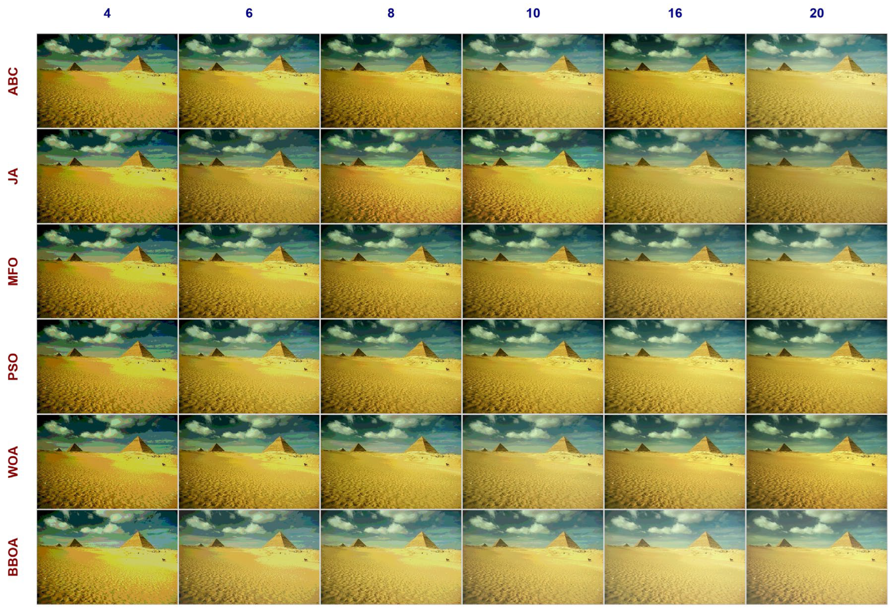
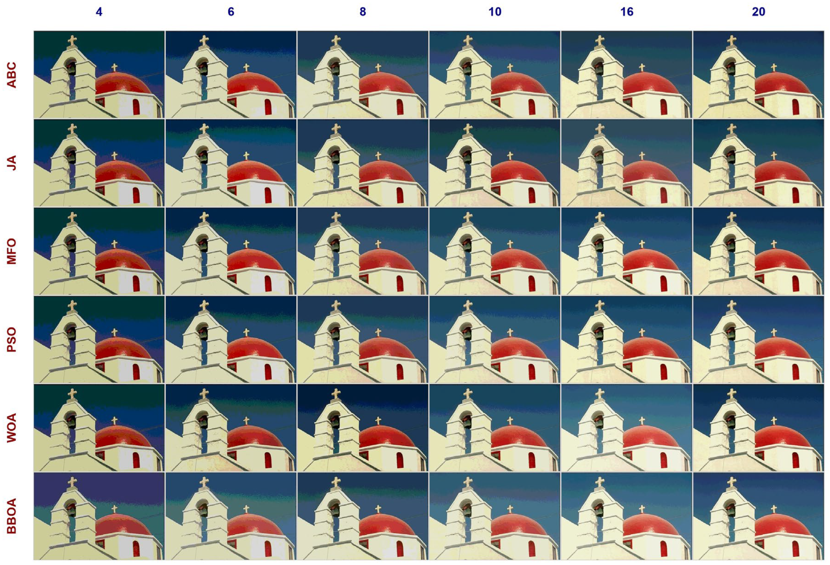
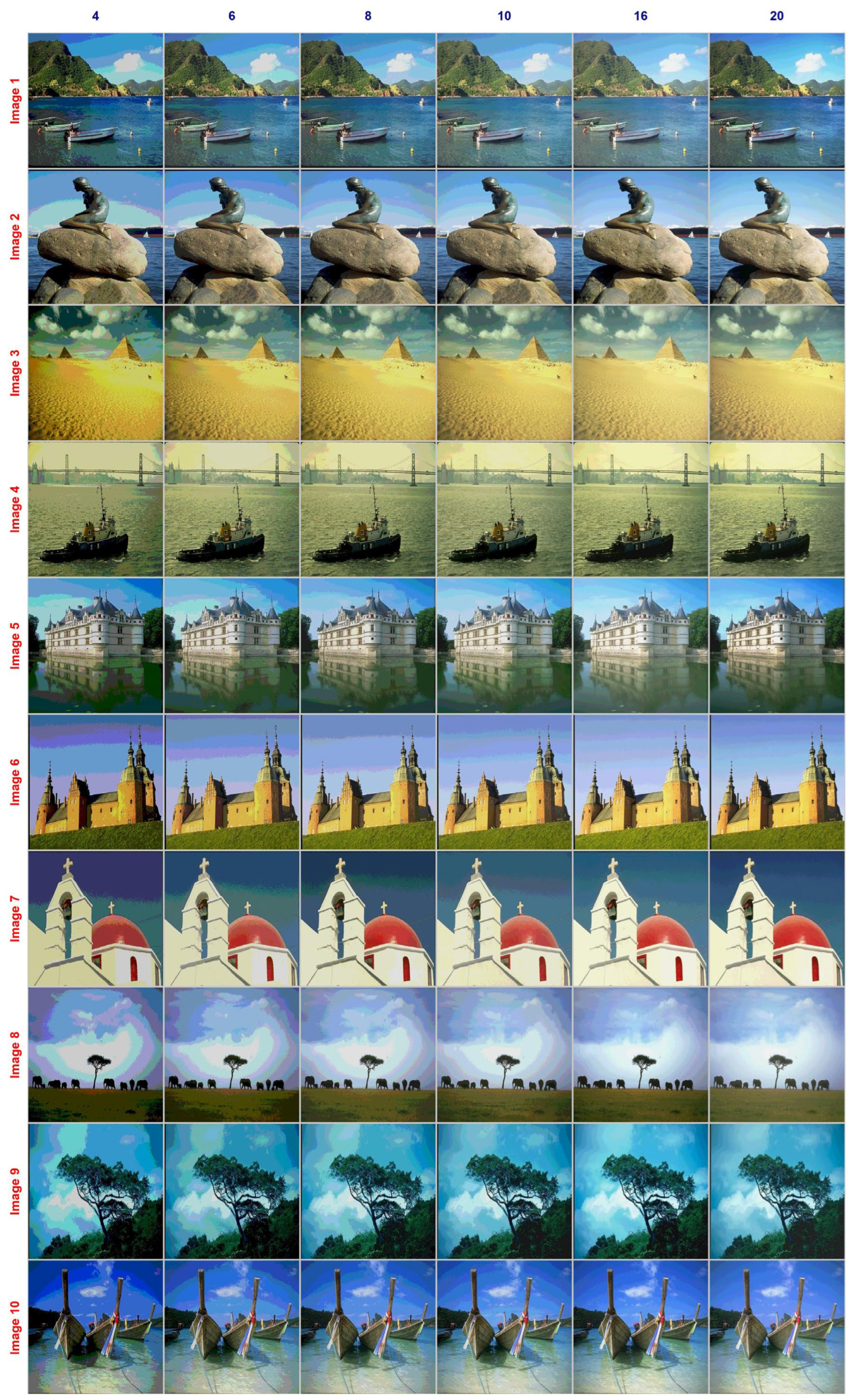
Figure 3. Comparison of segmented image 1 with Otsu’s method, along with optimization techniques ABC, JA, MFO, PSO, WOA, and the proposed method BBOA_S with N = 4, 6, 8, 10, 16 and 20.
Symmetry 18 00795 g003
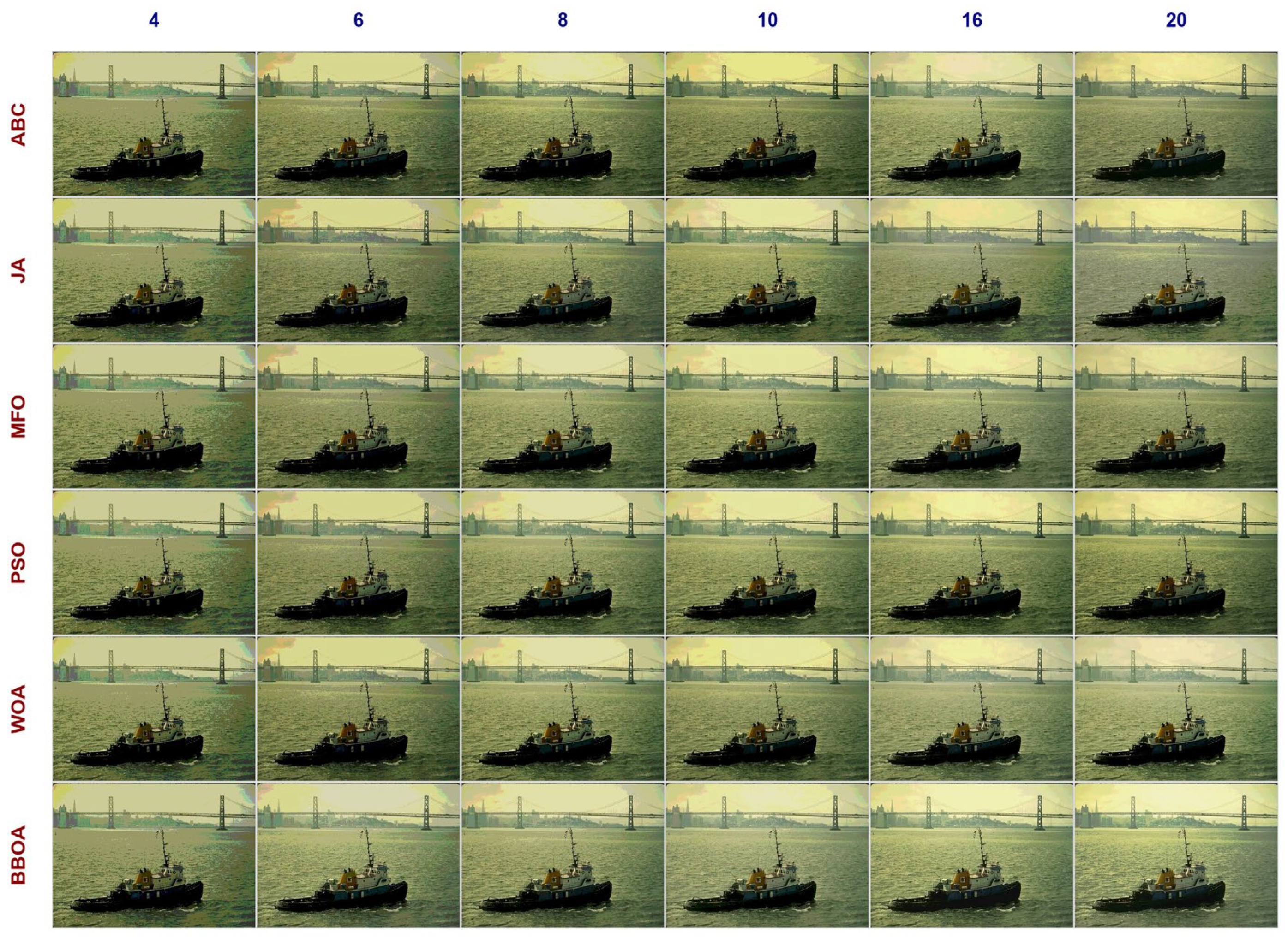
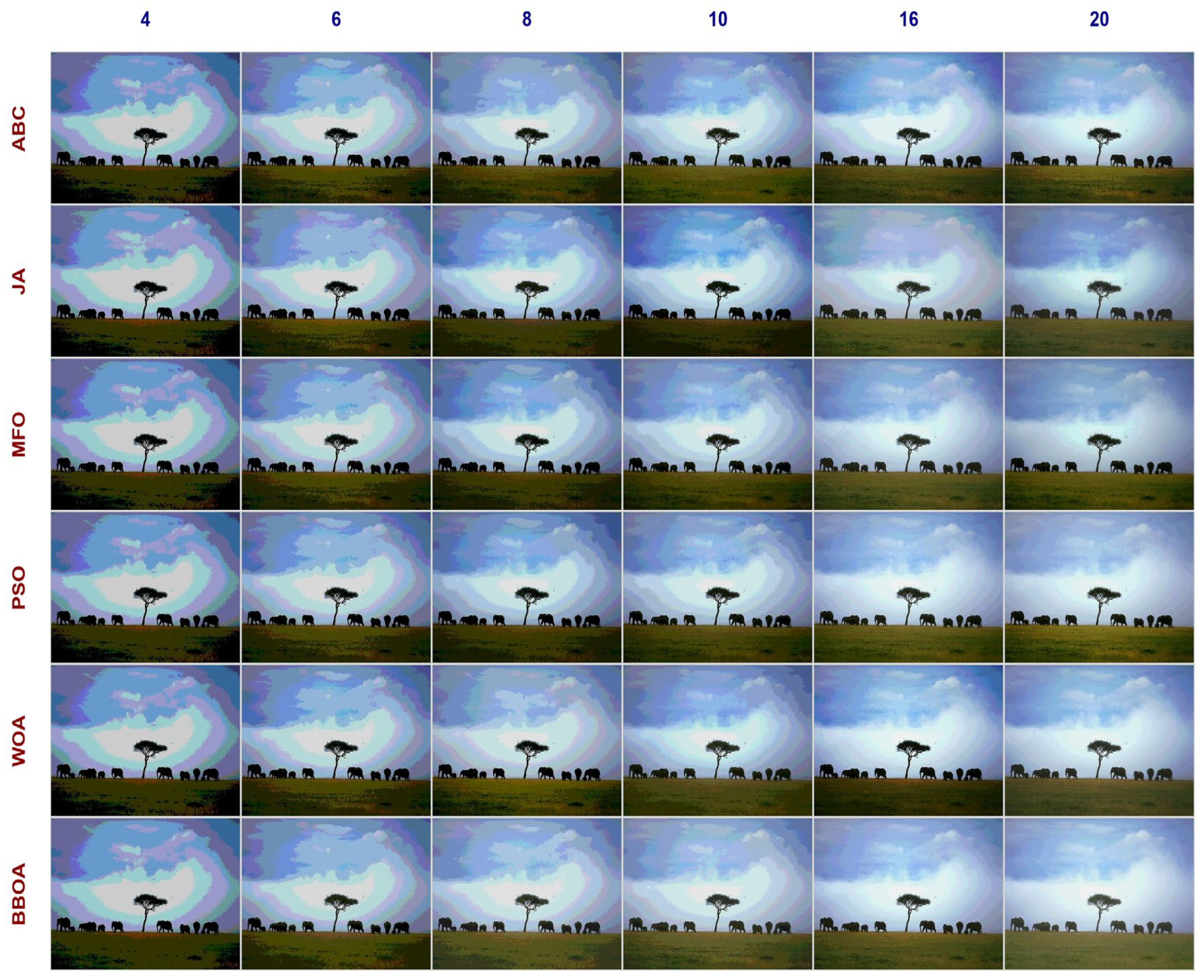
Figure 4. Comparison of segmented image 2 with Otsu’s method, along with optimization techniques ABC, JA, MFO, PSO, WOA, and the proposed method with BBOA for thresholds N = 4, 6, 8, 10, 16 and 20.
Symmetry 18 00795 g004
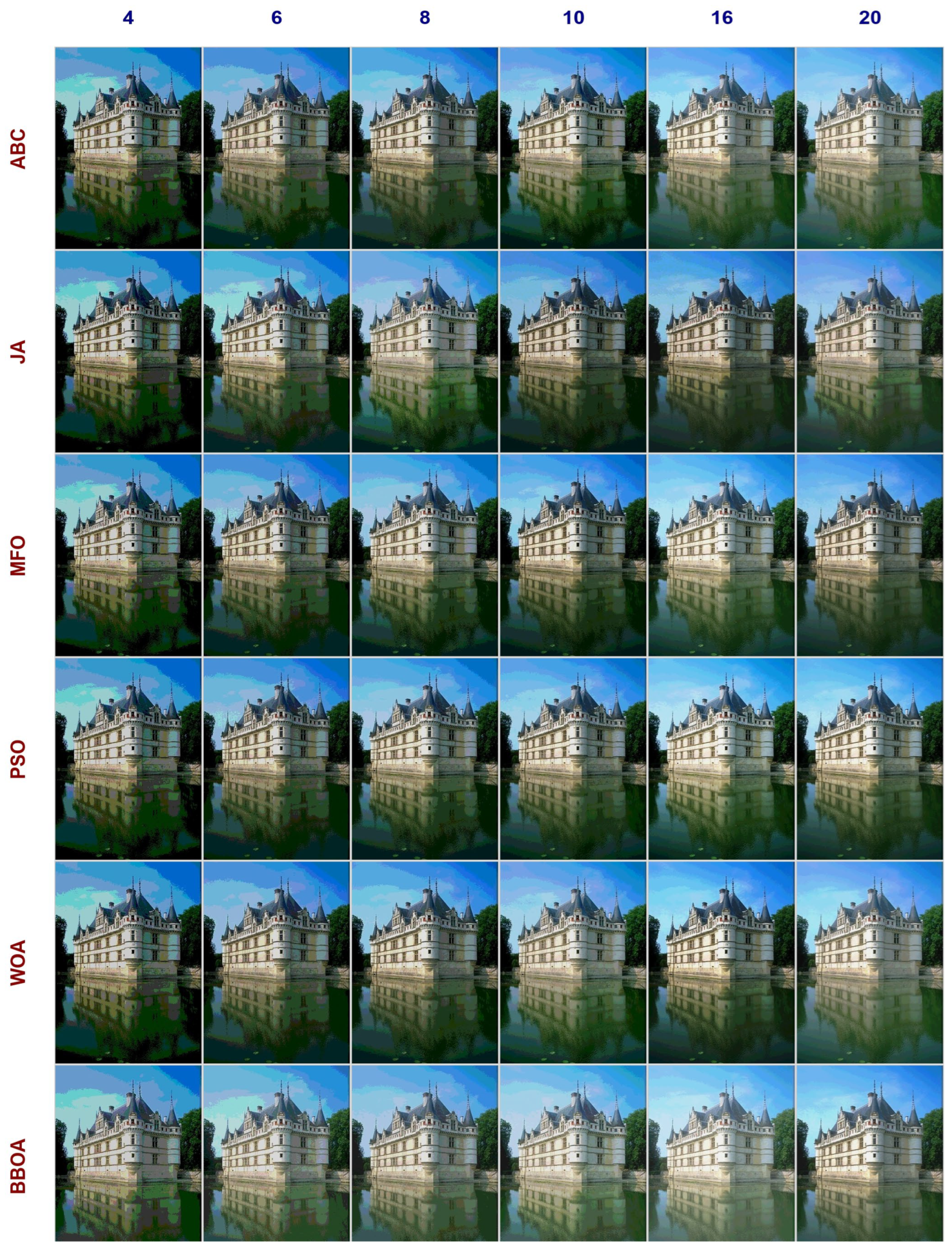
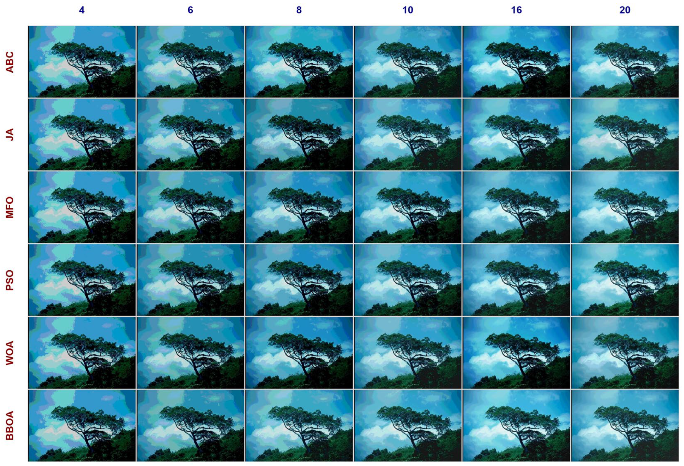
Figure 5. Comparison of segmented image 3 with Otsu’s method, along with optimization techniques ABC, JA, MFO, PSO, WOA, and the proposed method with BBOA for thresholds N = 4, 6, 8, 10, 16 and 20.
Symmetry 18 00795 g005
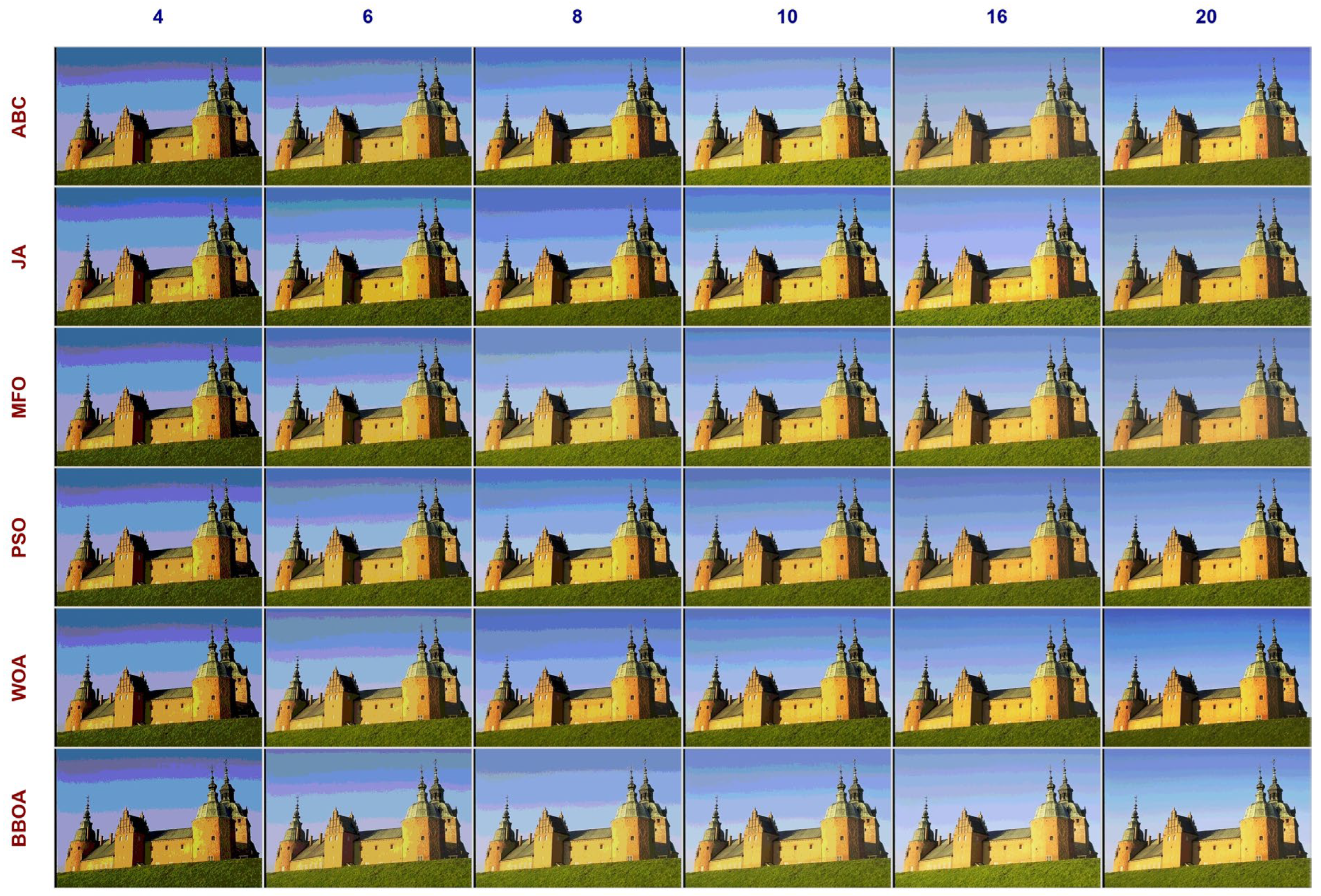
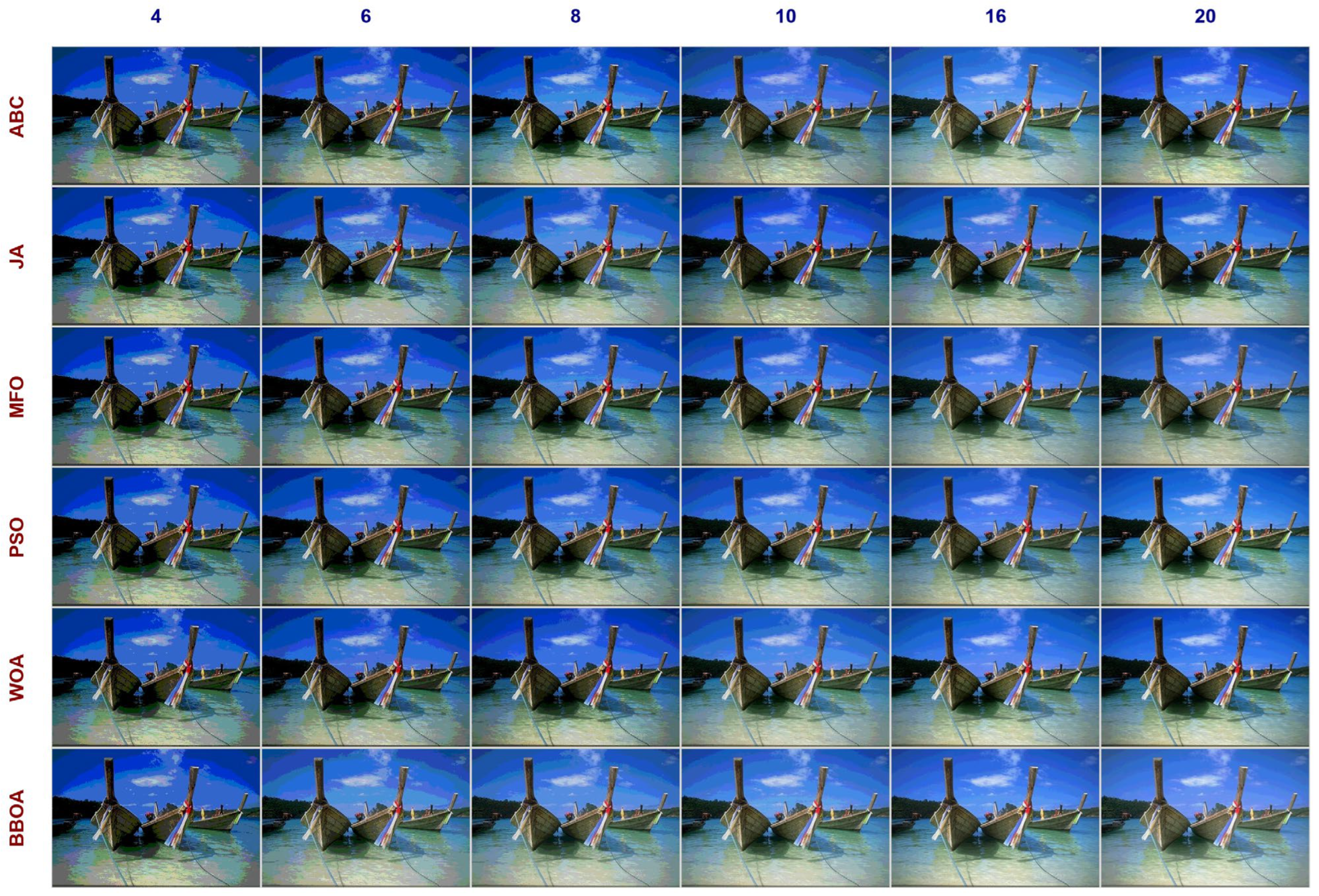
Figure 6. Comparison of segmented image 4 with Otsu’s method, along with optimization techniques ABC, JA, MFO, PSO, WOA, and the proposed method with BBOA for thresholds N = 4, 6, 8, 10, 16, and 20.
Symmetry 18 00795 g006
Figure 7. Comparison of segmented image 5 with Otsu’s method, along with optimization techniques ABC, JA, MFO, PSO, WOA, and the proposed method with BBOA for thresholds N = 4, 6, 8, 10, 16, and 20.
Symmetry 18 00795 g007
Figure 8. Comparison of segmented image 6 with Otsu’s method, along with optimization techniques ABC, JA, MFO, PSO, WOA, and the proposed method BBOA_S for thresholds N = 4, 6, 8, 10, 16 and 20.
Symmetry 18 00795 g008
Figure 9. Comparison of segmented image 7 with Otsu’s method, along with optimization techniques ABC, JA, MFO, PSO, WOA, and the proposed method BBOA_S for thresholds N = 4, 6, 8, 10, 16 and 20.
Symmetry 18 00795 g009
Figure 10. Comparison of segmented image 8 with Otsu’s method, along with optimization techniques ABC, JA, MFO, PSO, WOA, and the proposed method BBOA_S for thresholds N = 4, 6, 8, 10, 16 and 20.
Symmetry 18 00795 g010
Figure 11. Comparison of segmented image 9 with Otsu’s method, along with optimization techniques ABC, JA, MFO, PSO, WOA, and the proposed method BBOA_S for thresholds N = 4, 6, 8, 10, 16 and 20.
Symmetry 18 00795 g011
Figure 12. Comparison of segmentedimage10 with Otsu’s method, along with optimization techniques ABC, JA, MFO, PSO, WOA, and the proposed method BBOA_S for thresholds N = 4, 6, 8, 10, 16, and 20.
Symmetry 18 00795 g012
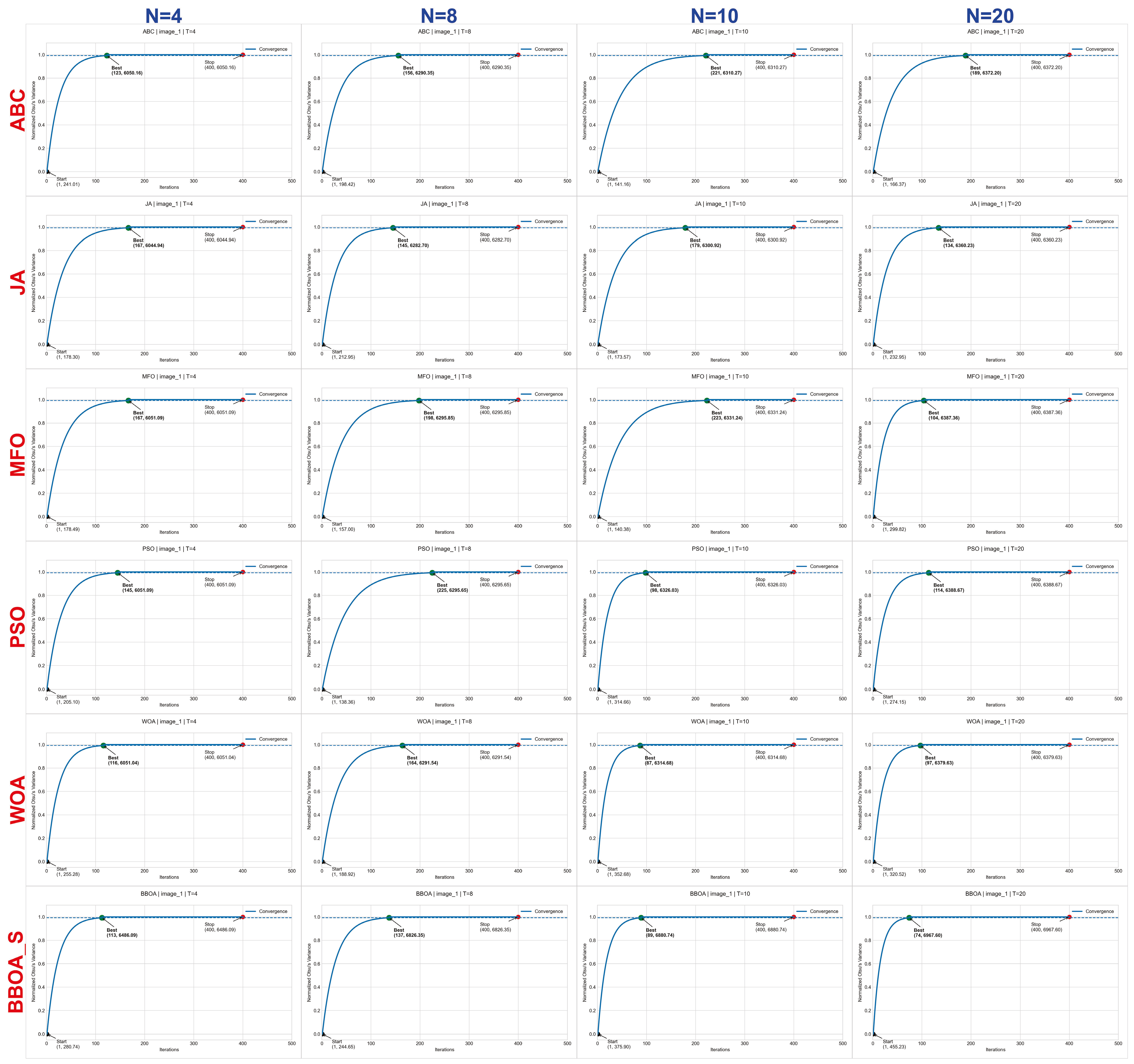
Figure 14 presents the convergence behavior of different optimization techniques for image 1 at various threshold levels (N = 4, 8, 10, and 20). From the plots, it is evident that the proposed BBOA_S method demonstrates faster and more stable convergence compared to ABC, JA, MFO, PSO, and WOA. While most algorithms gradually approach the optimal solution, BBOA_S reaches near-optimal fitness values in fewer iterations and maintains a smooth convergence trend without significant fluctuations. Additionally, the final converged value achieved by BBOA_S is consistently better (higher fitness) across all threshold levels, indicating improved optimization capability. This behavior highlights the strong exploration–exploitation balance of the proposed method, enabling it to avoid local minima and achieve superior segmentation performance efficiently. Overall, the convergence curves clearly validate that BBOA_S is more reliable, faster, and effective than the compared algorithms.
It is clear from the thorough experimental study that the suggested BBOA_S-based segmentation framework consistently and significantly improves important quality measures, including PSNR, MSE, and SSIM. While the robust global search capacity of BBOA allows for efficient exploration and exploitation of the threshold search space, the combination of RGB and Sobel-based information improves edge preservation and contrast discrimination. The total quantitative and qualitative results unequivocally demonstrate the robustness, stability, and superiority of the suggested BBOA_S methodology for multilevel picture segmentation, even though FSIM values are still similar with those of current methods.
Figure 13. Comparison of segmented image 1 with image 10 with Otsu’s method, along with the proposed method BBOA_S for thresholds N = 4, 6, 8, 10, 16 and 20.
Symmetry 18 00795 g013
Figure 14. Comparison of the convergence curve of image 1 with Otsu’s method based on optimization techniques ABC, JA, MFO, PSO, and WOAwith Proposed Model BBOA_S.
Symmetry 18 00795 g014
Figure 15. Comparison of PSNR for 10 segmented images with Otsu’s method, along with optimization techniques ABC, JA, MFO, PSO, WOA, and the proposed method with BBOA for thresholds N = 4, 6, 8, 10, 16, and 20.
Symmetry 18 00795 g015
Figure 16. Comparison of average PSNR for segmented images image 10 with Otsu’s method, along with optimization techniques ABC, JA, MFO, PSO, WOA, and the proposed method BBOA_S for thresholds N = 4, 6, 8, 10, 16 and 20.
Symmetry 18 00795 g016
Figure 17. Comparison of verage SSIM for segmented images image 10 with Otsu’s method, along with optimization techniques ABC, JA, MFO, PSO, WOA, and the proposed method with BBOA for thresholds N = 4, 6, 8, 10, 16 and 20.
Symmetry 18 00795 g017
Table 9. Comparison of average PSNR, MSE, SSIM, and DSC of 100 segmented with Otsu’s method based on optimization technique ABC, JA, MFO, PSO, and WOA with Proposed Model BBOA_S for 100 images for thresholds with N = 4, 6, 8, 10, 16 and 20.
Different Methods
METRICSABCJAMFOPSOWOABBOA_S
PSNR21.577521.636621.655421.906721.677223.2442
MSE637.7787663.574640.639592.6881639.9682464.3813
SSIM0.9470.94740.94780.94850.94920.9716
DSC0.9350.9410.93560.93220.93630.9595

7. Conclusions

This paper presents a novel image segmentation framework based on the multilevel image segmentation approach, based on Otsu’s method through the application of the optimization technique and Sobel filter to find optimized threshold values. The proposed algorithm combines Otsu’s image thresholding technique with the Brown Bear Optimization Algorithm (BBOA_S) and Sobel operator-based information, and it is experimented on 100 images. The proposed algorithm has been tested on ten different natural color benchmark images. The results demonstrate the proposed algorithm’s strength in image segmentation by performing better than the competing algorithms, including ABC, JA, MFO, PSO, and WOA. The proposed algorithm has an average PSNR of 23.24, which is higher than the PSNR obtained by the competing algorithms, including ABC (21.57), JA (21.63 dB), MFO (21.654), PSO (21.9), and WOA (21.6772). The proposed algorithm minimizes the error by achieving the lowest MSE. The proposed algorithm achieves an average SSIM of 0.9716, which is the best among the results obtained by the competing algorithms. The results obtained by the proposed algorithm are better than the results obtained by the competing algorithms, which gives a better DSC value of 0.9595. In conclusion, the proposed method demonstrates improved segmentation performance in terms of structural preservation and quality metrics. This work aims to improve robustness and efficiency by incorporating advanced edge detectors, such as Canny, and by utilizing color edge information directly from RGB channels. Hybrid or adaptive optimization strategies can also be explored to enhance convergence and reduce parameter dependency.

Supplementary Materials

The following supporting information can be downloaded at: https://drive.google.com/drive/folders/12is0nz2KI87VPpZHdyMHNlIJbzAH2Imt?usp=drive_link (accessed on 27 April 2026).

Author Contributions

Conceptualization, D.S.M. and K.P.C.; methodology, D.S.M. and K.P.C.; software, D.S.M.; validation, K.P.C.; formal analysis, D.S.M.; investigation, D.S.M. and K.P.C.; resources, D.S.M.; data curation, D.S.M.; writing—original draft preparation, D.S.M.; writing—review and editing, D.S.M. and K.P.C.; visualization, D.S.M.; supervision, K.P.C. All authors have read and agreed to the published version of the manuscript.

Funding

This research received no external funding.

Data Availability Statement

The original contributions presented in this study are included in the article. Further inquiries can be directed to the corresponding author.

Conflicts of Interest

The authors declare no conflicts of interest.

References

  1. Zaitoun, N.M.; Aqel, M.J. Survey on Image Segmentation Techniques, Procedia Computer Science. Procedia Comput. Sci. 2015, 65, 797–806. [Google Scholar] [CrossRef] [Scilit]
  2. Moorthy, J.; Gandhi, U.D. A Survey on Medical Image Segmentation Based on Deep Learning Techniques. Big Data Cogn. Comput. 2022, 6, 117. [Google Scholar] [CrossRef] [Scilit]
  3. Singh, S.; Mittal, N.; Singh, H. A multilevel thresholding algorithm using LebTLBO for image segmentation. Neural Comput. Appl. 2020, 32, 16681–16706. [Google Scholar] [CrossRef] [Scilit]
  4. Shi, L.; Wang, G.; Mo, L.; Yi, X.; Wu, X.; Wu, P. Automatic Segmentation of Standing Trees from Forest Images Based on Deep Learning. Sensors 2022, 22, 6663. [Google Scholar] [CrossRef] [Scilit] [PubMed]
  5. Otsu, N. A threshold selection method from gray-level histograms. IEEE Trans. Syst. Man Cybernet. 1979, 9, 62–66. [Google Scholar] [CrossRef] [Scilit]
  6. Shahid, K.T.; Schizas, I. Unsupervised Mitral Valve Tracking for Disease Detection in Echocardiogram Videos. J. Imaging 2020, 6, 93. [Google Scholar] [CrossRef] [Scilit]
  7. Patra, S.; Gautam, R.; Singla, A. A novel context-sensitive multilevel thresholding for image segmentation. Appl. Soft Comput. J. 2014, 23, 122–127. [Google Scholar] [CrossRef] [Scilit]
  8. Jia, H.; Ma, J.; Song, W. Multilevel Thresholding Segmentation for Color Image Using Modified Moth-Flame Optimization. IEEE Access 2019, 7, 44097–44134. [Google Scholar] [CrossRef] [Scilit]
  9. Liu, L.; Huo, J. Apple Image Recognition Multi-Objective Method Based on the Adaptive Harmony Search Algorithm with Simulation and Creation. Information 2018, 9, 180. [Google Scholar] [CrossRef] [Scilit]
  10. Resma, K.B.; Nair, M.S. Multilevel thresholding for image segmentation using Krill Herd Optimization algorithm. J. King Saud Univ. Comput. Inf. Sci. 2018, 33, 528–541. [Google Scholar] [CrossRef] [Scilit]
  11. Oliva, D.; Cuevas, E.; Pajares, G.; Zaldivar, D.; Osuna, V. A Multilevel Thresholding algorithm using electromagnetism optimization. Neurocomputing 2014, 139, 357–381. [Google Scholar] [CrossRef] [Scilit]
  12. ABhandari, A.; Kumar, A.; Chaudhary, S.; Singh, G. A novel color image multilevel thresholding-based segmentation using nature-inspired optimization algorithms. Expert Syst. Appl. 2016, 63, 112–133. [Google Scholar] [CrossRef] [Scilit]
  13. Tam, W.; Paul, B.; Alirezaie, J. Robust lung segmentation in Chest X-ray images using modified U-Net with deeper network and residual blocks. Comput. Methods Programs Biomed. Update 2025, 8, 100211. [Google Scholar] [CrossRef] [Scilit]
  14. Hammouche, K.; Diaf, M.; Siarry, P. A comparative study of various meta-heuristic techniques applied to the multilevel thresholding problem. Eng. Appl. Artif. Intell. 2010, 23, 676–688. [Google Scholar] [CrossRef] [Scilit]
  15. Wolper, D.H.; Macready, W.G. No free lunch theorems for optimization. IEEE Trans. Evol. Comput. 1997, 1, 67–82. [Google Scholar] [CrossRef] [Scilit]
  16. Karaboga, D.; Basturk, B. A powerful and efficient algorithm for numerical function optimization: Artificial bee colony (ABC) algorithm. J. Glob. Optim. 2007, 39, 459–471. [Google Scholar] [CrossRef] [Scilit]
  17. Mirjalili, S.; Mirjalili, S.M.; Lewis, A. Grey wolf optimizer. Adv. Eng. Softw. 2014, 69, 46–61. [Google Scholar] [CrossRef] [Scilit]
  18. Mirjalili, S. Moth-flame optimization algorithm: A novel nature-inspired heuristic paradigm. Knowl.-Based Syst. 2015, 89, 228–249. [Google Scholar] [CrossRef] [Scilit]
  19. Prakash, T.; Singh, P.P.; Singh, V.P.; Singh, S.N. A Novel Brown-bear Optimization Algorithm for Solving Economic Dispatch Problem. In Advanced Control & Optimization Paradigms for Energy System Operation and Management; River Publishers: Gistrup, Denmark, 2022; pp. 137–164. [Google Scholar] [CrossRef] [Scilit]
  20. Kumar, R.S.; Meera, P.S.; Lavanya, V.; Hemamalini, S. Brown bear optimized random forest model for short term solar power forecasting. Results Eng. 2025, 25, 104583. [Google Scholar] [CrossRef] [Scilit]
  21. Bairooz, J.J.; Mardukhi, F. An Innovative Enhanced JAYA Algorithm for the Optimization of Continuous and Discrete Problems. Algorithms 2024, 17, 472. [Google Scholar] [CrossRef] [Scilit]
  22. Abu Zitar, R. A Review of the Genetic Algorithm and JAYA Algorithm Applications. In Proceedings of the 2022 15th International Congress on Image and Signal Processing, BioMedical Engineering and Informatics (CISP-BMEI), Beijing, China, 5–7 November 2022; pp. 1–7. [Google Scholar] [CrossRef] [Scilit]
  23. Yang, X.-S. Multiobjective firefly algorithm for continuous optimization. Eng. Comput. 2013, 29, 175–184. [Google Scholar] [CrossRef] [Scilit]
  24. Chen, K.; Zhou, Y.; Zhang, Z.; Dai, M.; Chao, Y.; Shi, J. Multilevel image segmentation based on an improved firefly algorithm. Math. Probl. Eng. 2016, 2016, 1578056. [Google Scholar] [CrossRef] [Scilit]
  25. Fan, Q.; Ma, Y.; Wang, P.; Bai, F. Otsu Image Segmentation Based on a Fractional Order Moth–Flame Optimization Algorithm. Fractal. Fract. 2024, 8, 87. [Google Scholar] [CrossRef] [Scilit]
  26. Akay, B. A study on particle swarm optimization and artificial bee colony algorithms for multilevel thresholding. Appl. Soft Comput. 2013, 13, 3066–3091. [Google Scholar] [CrossRef] [Scilit]
  27. Khairuzzaman, A.K.M.; Chaudhury, S. Multilevel thresholding using grey wolf optimizer for image segmentation. Expert Syst. Appl. 2017, 85, 64–76. [Google Scholar] [CrossRef] [Scilit]
  28. Yang, S.; Zhang, G.; Zheng, B.; Zhou, X.; Zhang, J.; Heidari, A.A.; Chen, H.; Miao, X. Gaussian bare-bone JAYA algorithm for multi-threshold medical image segmentation. Sci. Rep. 2025, 15, 42658. [Google Scholar] [CrossRef] [Scilit] [PubMed]
  29. Wang, J.; Bei, J.; Song, H.; Zhang, H.; Zhang, P. A whale optimization algorithm with combined mutation and removing similarity for global optimization and multilevel thresholding image segmentation. Appl. Soft Comput. 2023, 137, 110130. [Google Scholar] [CrossRef] [Scilit]
  30. Khehra, B.S.; Singh, A.; Kaur, L. Whale Optimization Algorithm for Color Image Segmentation using Supra-Extensive Entropy. In Proceedings of the 2022 IEEE Canadian Conference on Electrical and Computer Engineering (CCECE), Halifax, NS, Canada, 18–20 September 2022; pp. 395–401. [Google Scholar] [CrossRef] [Scilit]
  31. Ahmed, S.; Biswas, A. A cross-entropy and whale optimization algorithm-based image segmentation for aerial images. Int. J. Inf. Technol. 2025, 17, 5313–5327. [Google Scholar] [CrossRef] [Scilit]
  32. Fedor, B.; Straub, J. A Particle Swarm Optimization Backtracking Technique Inspired by Science-Fiction Time Travel. AI 2022, 3, 390–415. [Google Scholar] [CrossRef] [Scilit]
  33. Huo, F.; Wang, Y.; Ren, W. Improved artificial bee colony algorithm and its application in image threshold segmentation. Multimed. Tools Appl. 2022, 81, 2189–2212. [Google Scholar] [CrossRef] [Scilit]
  34. Kumar, S.; Kumar, S.; Kumar, B.; Sharma, S.; Chaudhary, H. Optimization Methods for Image Edge Detection Using Ant and Bee Colony Techniques. In Advances in Information Communication Technology and Computing; Goar, V., Kuri, M., Kumar, R., Senjyu, T., Eds.; Lecture Notes in Networks and Systems; Springer: Singapore, 2023; Volume 628. [Google Scholar] [CrossRef] [Scilit]
  35. Chavan, M.; Varadarajan, V.; Gite, S.; Kotecha, K. Deep Neural Network for Lung Image Segmentation on Chest X-ray. Technologies 2022, 10, 105. [Google Scholar] [CrossRef] [Scilit]
  36. Kubicek, J.; Varysova, A.; Cerny, M.; Hancarova, K.; Oczka, D.; Augustynek, M.; Penhaker, M.; Prokop, O.; Scurek, R. Performance and Robustness of Regional Image Segmentation Driven by Selected Evolutionary and Genetic Algorithms: Study on MR Articular Cartilage Images. Sensors 2022, 22, 6335. [Google Scholar] [CrossRef] [Scilit] [PubMed]
  37. Abak, A.T.; Baris, U.; Sankur, B. The performance evaluation of thresholding algorithms for optical character recognition. In Proceedings of the Fourth International Conference on Document Analysis and Recognition, Ulm, Germany, 18–20 August 1997; Volume 2, pp. 10–13. [Google Scholar]
  38. Gu, K.; Liu, H.; Gao, Y.; Wang, C.; Wong, L.-K.; Lin, W.; Zhai, G.; Zhang, W.; Thalmann, D. Infrared Image Quality Estimation with Node-to-Graph Regression. IEEE Trans. Multimed. 2026, 28, 2238–2252. [Google Scholar] [CrossRef] [Scilit]
  39. Al-Dayel, I.; Nadeem, M.F.; Bashir, Y.; Shabbir, A. Information-Theoretic Medical Image Encryption via LLE-Verified Chaotic Keystreams and DNA Diffusion. Entropy 2025, 27, 1149. [Google Scholar] [CrossRef] [Scilit] [PubMed]
  40. Zhang, H.; Zhong, Q.; Liu, J.; Chen, R.; Wang, Z. SAFARI-net: Scale-adaptive frequency aware refinement infrastructure for infrared small target detection. Opt. Laser Technol. 2026, 199, 115049. [Google Scholar] [CrossRef] [Scilit]
Figure 1. Input image considered for experimentation along with histograms. Plots of red, green, and blue indicate histograms of red, green, and blue components of the color image.
Symmetry 18 00795 g001
Disclaimer/Publisher’s Note: The statements, opinions and data contained in all publications are solely those of the individual author(s) and contributor(s) and not of MDPI and/or the editor(s). MDPI and/or the editor(s) disclaim responsibility for any injury to people or property resulting from any ideas, methods, instructions or products referred to in the content.