Development of an Assembly Sequence Planning and Simulation System Based on Assembly Accuracy

Abstract

Assembly represents the culminating phase in the product production cycle, accounting for over 40% of production costs. Conventional assembly sequence planning methodologies predominantly prioritize geometric feasibility, tool change frequency, and directional change frequency as primary optimization objectives. Assembly accuracy is rarely systematically considered during the planning phase; instead, it is typically evaluated and optimized retrospectively after the production sequence has been established, making it difficult to effectively mitigate cumulative tolerances. During physical prototyping, failure to meet accuracy standards necessitates re-planning, which delays progress and increases costs. We propose an algorithm that integrates assembly accuracy prediction directly into the assembly sequence generation process. This enables sequence planning to be driven by constraints related to both assembly accuracy and efficiency. First, assembly precedence relationships are established based on the assembly information matrix to identify the base components. During the disassembly process, disassembly feasibility checks are incorporated to prevent the creation of isolated parts with no contact points, thereby enhancing the engineering soundness of the precedence modeling. Second, we propose an improved greedy topological sorting algorithm that incorporates assembly accuracy predictions as a key constraint in the objective function; by merging symmetrical parts in the prediction model to reduce the search space, the algorithm ultimately generates an assembly sequence that balances geometric feasibility, assembly efficiency, and assembly accuracy. Finally, we developed an integrated virtual assembly simulation system that combines assembly information extraction, sequence planning, and accuracy calculation, enabling the rapid generation and closed-loop verification of high-precision assembly sequences. Utilizing a simplified model as a case study, we generate comparison sequences with and without accuracy prediction and validate them through virtual assembly simulation. The experimental results show that, compared to traditional assembly sequences that do not account for precision, the proposed method improves the assembly precision pass rate by approximately 23% while maintaining assembly efficiency and significantly reduces the risk of rework and re-assembly caused by improper sequencing. Simulation software developed using this method can accurately plan assembly sequences for 25 parts in 223.58 s.

1. Introduction

Assembly is the final stage in the product production cycle, and assembly quality largely determines the final quality of the product. Assembly precision is one of the key indicators for evaluating product assembly quality [1,2]. Driven by modern manufacturing models and technologies such as concurrent engineering, computer-integrated manufacturing systems, and virtual manufacturing, intelligent assembly has become one of the core drivers of manufacturing development. Virtual assembly, as the core component in achieving intelligent assembly, holds significant value in enabling low-cost, high-efficiency, and short-cycle completion of component assembly and forming [3]. This approach has been demonstrated to substantially enhance the quality and efficiency of product design and manufacturing.

Assembly sequence planning (ASP) represents a pivotal technological advancement within the domain of virtual assembly research, with its fundamental objective being the formulation of feasible part assembly sequences within a virtual environment [4]. Assembly sequence planning is an NP-hard problem that is prone to combinatorial explosion as the number of parts increases [5,6,7]. Therefore, researchers typically use intelligent optimization algorithms to solve this problem.

Existing research has primarily focused on methods based on heuristic and intelligent optimization algorithms [8,9]. Common methods include particle swarm optimization, genetic algorithms, and ant colony optimization [10]. Bonneville et al. [11] were the first to introduce genetic algorithms into the field of assembly sequence planning, achieving automatic optimization of assembly sequences. Subsequently, Chica et al. [12] applied the ant colony optimization algorithm to the assembly sequence planning process with a view to enhancing search efficiency and solution quality. Saeed et al. [13] employed an optimization-based method to address the problem of estimating assembly sequence execution times. Sheng et al. [14] employed a Symbiotic Organism Search (SOS) algorithm combined with a diversification strategy to address feasibility constraints and cost optimization in assembly sequence planning. Hong Yu et al. [15] conducted a comparative analysis of the performance of particle swarm optimization and genetic algorithms in assembly sequence planning, thereby verifying the advantages of the particle swarm algorithm in terms of convergence speed and global search capability. While these methods perform well in terms of computational efficiency, their search process relies on randomness, making them prone to getting stuck in local optima under complex constraints [16].

To address these issues, some scholars have proposed improved or hybrid algorithms. Liang Lifen et al. [17] incorporated a chaotic search mechanism into the particle swarm optimization algorithm to enhance its ability to escape local optima. Ding Yujin et al. [18] employed a modified particle swarm optimization algorithm—featuring chaotic initialization, nonlinear inertial weights, and asymmetric learning factors—to address the combinatorial explosion and local optima problems. Wan et al. [19] employed a multi-optimal genetic algorithm combined with a flexible programming method for assembly sequencing to address the issue that assembly sequencing typically yields only a single optimal solution, whereas actual production requires flexible adjustments to the sequence. Huang Fengyun [20] used a hybrid strategy involving alternating iterations of the Imperial Competition Algorithm and the genetic algorithm. Zhang et al. [21] employed a hybrid SOS-PSO algorithm to address the issues of the algorithm getting stuck in local optima and parameter sensitivity in assembly sequence planning. Mutale et al. [22] used a hybrid Particle Swarm-Based Bacterial Foraging Optimization (PSBFO) algorithm to solve the assembly sequence. Ju et al. [23] employed a genetic-greedy combinatorial algorithm to address the combinatorial explosion and local optima problems in the sequence planning of cabin assembly for large cruise ships. In addition to heuristic algorithms for determining assembly sequences, there are also model-based methods for determining assembly sequences. While these methods have alleviated the local optimum problem to some extent, they still primarily focus on algorithmic optimization rather than reducing the size of the solution space by modeling actual operating conditions.

In addition, some studies have attempted to incorporate graph models or decision models into assembly sequence planning. Nagpal and Mehr [24] adopted a sequential decision-making framework that combines dynamic programming, a graph-search-based assembly planner, and a deep Q-network to address the combinatorial explosion and constraint satisfaction problems in robotic assembly sequence planning. Chen et al. [25] employed a parallel assembly sequence planning method that combines a graph model with ant colony optimization to address the issues of low efficiency and dependence on an initial feasible sequence in the assembly sequence planning of complex products. CHEN YANG et al. [26] employed interval dynamic modeling, non-probabilistic time-varying reliability constraints, and multi-objective optimization methods to solve the sequential planning problem for the in-orbit assembly of large-scale space structures under conditions of limited data. While these methods can improve the efficiency of solutions to some extent, they usually prioritize geometric feasibility or assembly costs as their main optimization objectives. Since assembly accuracy predictions are not incorporated into the sequence generation decision-making process, it is difficult to ensure that the final assembly meets design requirements in terms of accuracy.

Assembly accuracy is a key factor determining the performance of precision mechanical products. Current methods for predicting assembly accuracy primarily include mathematical modeling and analysis, error propagation and stochastic simulation, digital twins and data-driven approaches, as well as model reduction and accuracy decomposition. For example, Yang et al. [27] employed a method based on Isogeometric Analysis (IGA) and Non-Uniform Rational B-Splines (NURBS) to address the challenge of accurately predicting the coupled effects of non-ideal surface topography and part deformation in precision mechanical assemblies. Li et al. [28] utilized a virtual assembly method based on the reconstruction of measured surface topography, employing three matching strategies—high precision, high efficiency, and high yield—to address the challenges of assembly precision prediction and control. Janssen et al. [29] employed a modular order-reduction method based on relative modal importance and robustness analysis, decomposing assembly accuracy requirements top-down into component accuracy requirements, thereby resolving the issues of redundancy or insufficiency in traditional modal synthesis methods caused by neglecting inter-component coupling. These methods offer excellent geometric representation and deformation analysis accuracy; however, they place a strong emphasis on geometric–physical modeling, resulting in relatively high overall computational complexity.

To address these shortcomings, Zhao et al. [30] employed a method combining rigid–flexible coupling and a multidimensional vector loop to analyze assembly deformation deviations through equivalent analysis and establish a multi-source deviation propagation model, thereby resolving the issue of inaccurate assembly accuracy predictions caused by the neglect of deformation in weakly rigid components. Chen et al. [31] utilized a method based on error propagation and stochastic simulation to address the discrepancy between on-site assembly accuracy and design specifications resulting from the randomness of component manufacturing errors. However, the methods described above struggle to capture the dynamic changes that occur during the assembly process. For this reason, Lv et al. [32] employed a digital twin-driven dual-closed-loop optimization mechanism to construct a four-layer reference model comprising physical entities, virtual entities, twin data, and services, thereby resolving the difficulty of precision control during the assembly of complex products. Yi et al. [33] employed a digital twin-driven method for multi-source data fusion and error propagation analysis, resolving the issue of prediction inaccuracies caused by multidimensional error coupling in the high-precision assembly of complex products.

However, current assembly accuracy predictions primarily rely on measured data or complete geometric models, making it difficult to conduct them efficiently during the design phase, which results in accuracy issues being identified only at a later stage [34]. Zheng et al. [35] propose a method for planning the assembly sequence of complex products, which is based on an improved teaching–learning optimization algorithm. This method uses variable-step adaptive interference analysis to quickly verify the feasibility of assembly and automatically construct dimensional tolerance chains. Using cumulative assembly accuracy as the objective function and leveraging the improved algorithm’s global optimization capabilities, the method achieves highly precise optimization solutions for the assembly sequences of complex products. Building on this research, the present study further expands the optimization objectives to conduct multi-objective optimization that balances cumulative assembly accuracy and efficiency comprehensively. It integrates assembly accuracy prediction directly into the assembly sequence generation process, proactively mitigating tolerance accumulation at this stage. Additionally, it presents proprietary assembly sequence simulation and analysis software that enables the visual verification of sequence proposals and full-process simulation analysis. A comparison of our proposed method with those in the literature is shown in

Table 1. Comparison of the literature.

References	Key Research Focus	Our Proposed Methodology
[1]	Assembly simulation of an aircraft horizontal stabilizer using DELMIA.	Integrated assembly sequence planning and simulation.
[2]	Improving the seagull algorithm for ASP.	Using a deterministic greedy topological sorting algorithm.
[3]	The application of digital technology in mechanical design and manufacturing.	Focusing on the assembly sequence planning algorithm itself.
[4]	Ant colony optimization in ASP.	An improved topological sorting algorithm.
[5]	Multi-objective optimization methods for solving assembly process planning.	Optimizing the balance between accuracy and efficiency.
[6]	ASP of the discrete particle swarm optimization algorithm.	An improved topological sorting algorithm.
[7]	Thermal error modeling.	Modeling the propagation of assembly errors.
[8]	Genetic algorithms.	An improved topological sorting algorithm.
[9]	Research on production optimization.	We focus on deterministic sequence planning for multi-component products.
[10]	Soft computing methods for assembly sequence planning.	We propose a deterministic sequence planning method that incorporates accuracy calculations.
[11]	ASP of genetic algorithms.	Accuracy-based ASP.
[12]	The multi-objective ant colony optimization algorithm is used to estimate assembly time.	An improved topological algorithm that balances assembly accuracy, assembly efficiency, and geometric feasibility.
[13]	An optimization-based method for estimating the execution time of assembly sequences.	Focus on the accuracy of sequence generation.
[14]	ASP of the Symbiotic Organism Search Algorithm.	An improved topological sorting algorithm.
[15]	ASP for the particle swarm optimization algorithm.	A sequence planning algorithm that takes geometric feasibility into account.
[16]	Research feasible sequence generation and optimization methods.	Implement an ASP with built-in precision by using precision constraints as conditions.
[17]	Solving assembly sequences using an adaptive chaotic particle swarm algorithm.	Fast greedy topological sorting algorithm.
[18]	Improvements to the application of the particle swarm optimization algorithm in assembly sequence planning.	A topological algorithm that balances assembly accuracy.
[19]	ASP for multi-solution genetic algorithms.	Output only a single sequence that has been verified for both interference and accuracy.
[20]	ASP for the Union-Set Competition Algorithm.	We propose an improved topological algorithm that incorporates accuracy calculations.
[21]	ASP using a hybrid SOS-PSO algorithm.	We propose an improved topological algorithm that incorporates accuracy calculations.
[22]	Hybrid PSO-BFO algorithm.	We propose an improved topological algorithm that incorporates accuracy calculations.
[23]	Sequence planning using genetic algorithms for the optimization of cabins on large cruise ships.	A general framework for assembly planning.
[24]	Sequential decision-making.	Incorporate assembly accuracy into the decision-making process for sequence generation.
[25]	Based on automatic subassembly recognition and optimization search strategies.	Focus on assembly accuracy chain analysis.
[26]	Planning assembly sequences while considering topological constraints and vibration reliability.	By improving topological sorting, we achieve an explicit balance among geometric feasibility, efficiency, and accuracy.
[27]	Prediction of assembly accuracy based on isogeometric analysis.	Monte Carlo simulation based on the spinor model and coordinate transformations.
[28]	Predicting assembly accuracy using virtual assembly technology.	Accuracy prediction based on 3D models.
[29]	Optimize component combinations using modal selection methods.	Preliminary planning during the early stages of design.
[30]	Predicting assembly accuracy based on error propagation mechanisms.	Accuracy prediction of Monte Carlo random simulations based on the rotor model and coordinate system transformations.
[31]	Based on error propagation theory and stochastic simulation methods.	Sequence planning incorporates calculations of assembly accuracy.
[32]	A digital twin-driven design method for assembly Accuracy.	Quick prediction based on tolerances.
[33]	Digital twin accuracy prediction.	Direct geometric mapping method.
[34]	Research on human–robot collaboration.	Focus on assembly sequence planning.
[35]	Accuracy-oriented TLBO algorithm.	Based on an improved topological sorting algorithm, this approach directly integrates practical manufacturing constraints and precise calculations into the sequence generation process, balancing geometric feasibility, assembly efficiency, and assembly accuracy, and incorporates simulation software.
[36]	A method for generating interference-free assembly sequences based on 3D models.	Balancing assembly efficiency and precision.
[37]	A method for analyzing the stability of multi-path disassembly is proposed.	Automatic extraction and identification of part enclosures.
[38]	A disassembly method based on connection interfaces and motion calculators.	Human–machine interaction interference detection.
[39]	Sequence planning for disassembly based on an improved interference matrix.	Modeling assembly precedence relationships based on actual operating conditions.
[40]	Methods for assembly sequence planning and layout.	The connection matrix serves as the criterion for determining which rows can be split.
[41]	Apply the disassembly method to the virtual assembly system.	The disassembly method takes actual operating conditions into account.
[42]	Establishment of a diagram illustrating the propagation of errors in geometric elements.	Comprehensive error propagation diagram and Monte Carlo simulation.
[43]	A greedy algorithm for drones.	Greedy selection serves as an extension of the topological sort algorithm.

.

Traditional assembly sequence planning often treats accuracy evaluation as a post hoc step, failing to mitigate tolerance accumulation proactively during sequence generation. Furthermore, existing methods often fail to fully account for real-world operational constraints during the assembly precedence modeling phase. This results in assembly sequences that may include parts that do not come into contact with each other, thereby compromising the physical feasibility and practicality of the assembly process. Currently, there is no integrated simulation software that can combine interference detection, the automatic extraction of assembly information matrices, modeling of assembly precedence relationships, sequence planning, simulation animation generation, and assembly accuracy calculation. This makes it difficult to achieve rapid closed-loop verification from product models to feasible, high-precision sequences. To address these issues, we propose a drive-based planning method that integrates assembly accuracy prediction directly into the sequence generation process. First, during the assembly priority modeling phase, operational constraints are considered. An assembly priority graph is then constructed based on the assembly information matrix in order to identify base components. Dismantlability verification is incorporated into the disassembly process to prevent isolated parts being created with no contact, thereby enabling feasibility constraints to be screened for in advance. Secondly, an improved greedy topological sorting algorithm is proposed that incorporates assembly accuracy prediction as a key constraint in the objective function. This enables the generation of sequences that consider geometric feasibility, assembly efficiency and tolerance accumulation control simultaneously. Additionally, the accuracy prediction model merges symmetric parts to reduce the search space. Finally, a corresponding virtual assembly simulation system was developed to achieve integrated functionality ranging from interference detection to sequence generation, simulation animation, and accuracy calculation. This approach moves away from a post hoc accuracy evaluation model, enabling the generation of assembly sequences driven by the synergy of accuracy and efficiency.

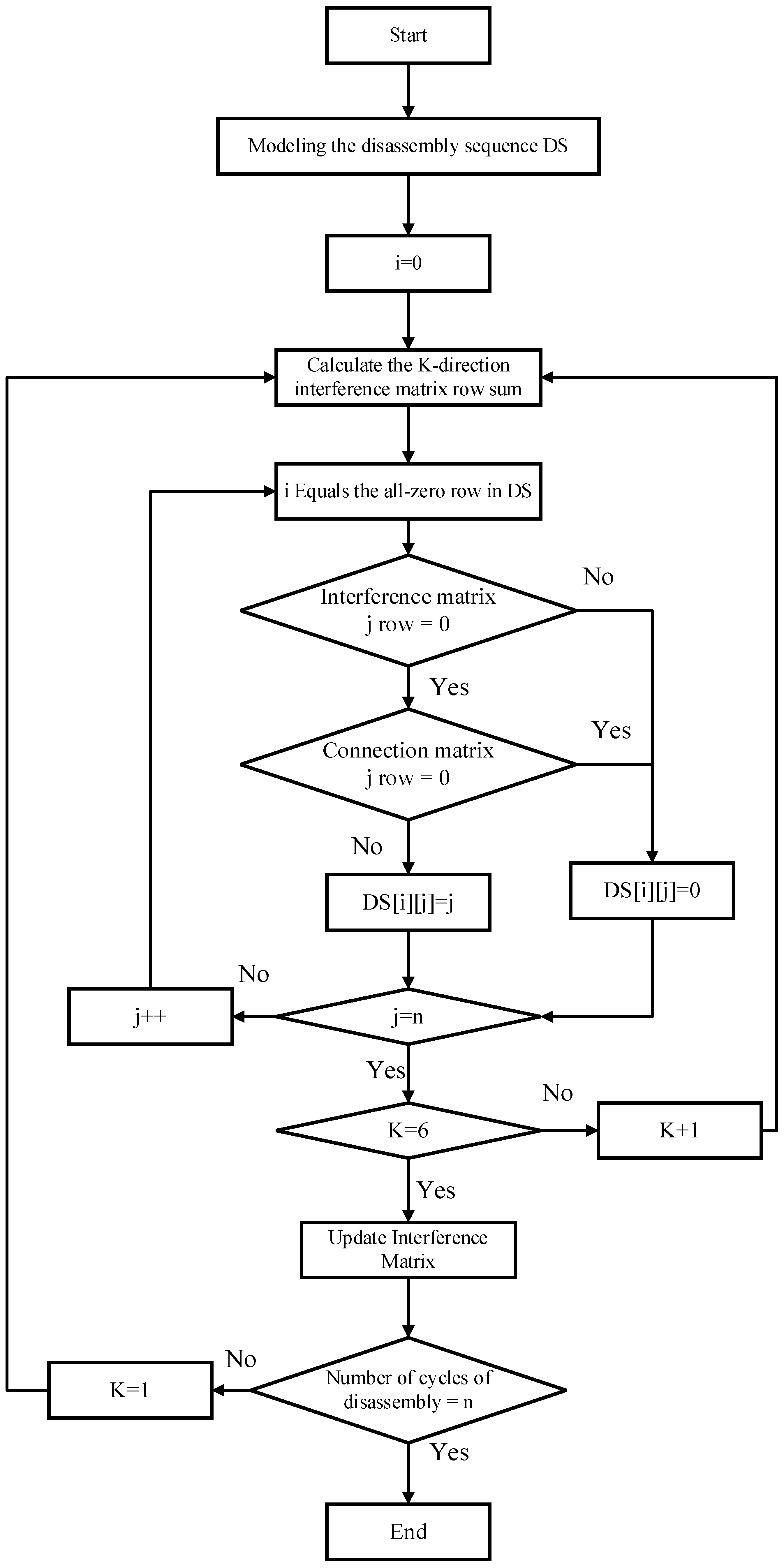
The remainder of this paper is structured as follows: Section 1 reviews the relevant literature, analyzes the shortcomings of existing methods for predicting assembly accuracy and sequence planning, and introduces the method we propose. Section 2 constructs a part relationship matrix through secondary development of Inte3D and interference checking to model assembly priority relationships. We address the issue that current algorithms used for solving assembly sequences search directly across the entire solution space and lack feasibility constraints. 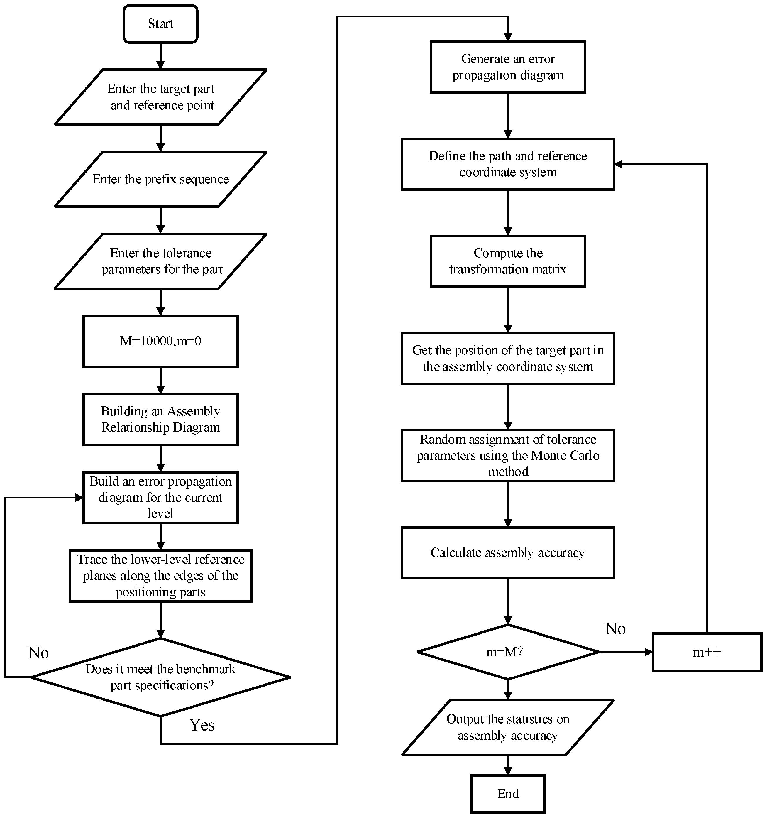In Section 3, a predictive model for assembly accuracy is established. This is achieved by constructing error propagation relationships based on the rotator model and coordinate system transformations. Statistical calculations are also performed using Monte Carlo simulation. This approach characterizes error accumulation during assembly and provides constraints for optimizing the assembly sequence.

Section 4 incorporates assembly accuracy prediction into an improved topological sorting algorithm to generate a comprehensively optimized assembly sequence by incorporating assembly accuracy predictions at an earlier stage, thereby addressing the shortcoming of traditional assembly sequence planning, which overlooks the impact of accuracy. In Section 5, we construct a comprehensive evaluation function to assess the quality of the assembly sequence. Section 6 introduces the simulation software developed for this purpose, which enables the fully automated generation of assembly sequences. Section 7 validates and evaluates the performance of the optimized sequence through specific case studies. Finally, the entire work is summarized.

2. Assembly Priority Relationship Model

Planning assembly sequences for complex products often suffers from inefficient solutions and compromised solution quality due to the vast search space and sparse distribution of feasible solutions. To address this issue, this study employs the geometrically feasible sequence inherent in the assembly priority relationship model as input for the optimization algorithm. This approach effectively accelerates the optimization process while ensuring that the sequence remains feasible.

2.1. Constructing the Interference Matrix

The interference matrix serves as a vital tool for describing the geometric constraints and spatial relationships between components within an assembly system. Its construction process is based on the intersection determination of component bounding boxes [36]. For an assembly containing n components, an n × n interference matrix I can be established. The matrix elements are defined in 0–1 format to represent the spatial interference relationship between any two components. The value assignment rules are shown in Equation (1) [37]:

$${\mathrm{I}}_{\mathrm{k}}[i][j]=\left\{\begin{array}{ll}1\hfill & \mathrm{Parts} i \mathrm{and} j \mathrm{interfere} \mathrm{in} \mathrm{the} \mathrm{k} \mathrm{direction}\hfill \\ 0\hfill & \mathrm{Parts} i \mathrm{and} j \mathrm{do} \mathrm{not} \mathrm{interfere} \mathrm{in} \mathrm{the} \mathrm{k} \mathrm{direction}\hfill \end{array}\right.$$

(1)

where the values of $i,j$ are in the range $0\le i\le n,0\le j\le n$. Let k denote the direction of the coordinate axes in a three-dimensional orthogonal Cartesian coordinate system, encompassing both the positive and negative directions of all principal axes. kdenotes the interference detection direction, $\mathrm{k}\in \left\{x_{+},y_{+},z_{+},x_{-},y_{-},z_{-}\right\}$, which corresponds, in order, to the positive direction of the x-axis, the positive direction of the y-axis, the positive direction of the z-axis, the negative direction of the x-axis, the negative direction of the y-axis, and the negative direction of the z-axis. Movement along a coordinate axis takes two basic forms: movement in the positive direction of the axis and movement in the negative direction of the axis.

The steps for constructing the interference matrix are as follows:

• Determine the interference detection interval. We select the assembly’s bounding dimensions as the interference detection interval [38].
• Establish the detection procedure. Create a new assembly step and import all part models of the assembly into this step.
• Perform displacement detection along specified directions. Select part i and displace it along direction k. Determine whether geometric interference occurs with other parts. The displacement matrix T is defined as in Equation (2):

$$T=\left[\begin{array}{ccc}{P}_x& P_y& P_z\end{array}\right]$$

(2)

Px, Py, and Pz represent the displacement along the three coordinate axes, respectively.

4.

Delete detection step. After traversing all parts to complete interference detection, delete this temporary step to obtain the interference matrix in the k direction.

5.

Iterate through three-dimensional directions. Execute the above steps along the x, y, and z directions to obtain the corresponding directional interference matrices. When part i moves along the k-direction and interferes with part j, part j moving along the negative k-direction will also interfere with part i. Therefore, the interference matrix for the negative direction is the transpose of the interference matrix for the positive direction.

2.2. Assembly Priority Matrix

Based on assembly practice, we define the part providing the most support as the base component, meaning the base component should be the part offering the greatest support to other components in the direction of gravity. The support relationship between parts must satisfy two conditions simultaneously: physical contact exists, and interference occurs in the direction of gravity. The support matrix S is logically derived from the gravity–direction interference matrix and the connection matrix L, with its element values determined according to Equation (3) [39]:

$$\mathrm{S}[i][j]=\left\{\begin{array}{ll}1\hfill & {\mathrm{I}}_g[i][j]=\mathrm{L}[i][j]=1\hfill \\ 0\hfill & \mathrm{else}\hfill \end{array}\right.$$

(3)

When the matrix element S[i][j] = 1, it indicates that part i provides support to part j. The connection matrix L is determined by the static interference check of the assembly, where the displacement matrix is zero. The definition criteria for the connection matrix are specified as in Equation (4) [40]:

$$\mathrm{L}[i][j]=\left\{\begin{array}{ll}1\hfill & \mathrm{Parts} i \mathrm{and} j \mathrm{are} \mathrm{connected}\hfill \\ 0\hfill & \mathrm{Parts} i \mathrm{and} j \mathrm{are} \mathrm{not} \mathrm{connected}\hfill \end{array}\right.$$

(4)

The criteria for determining the base component are as follows: Calculate the cumulative sum of each row element in the support matrix S. This cumulative sum represents the total number of parts supported by the corresponding component. The part corresponding to the row with the maximum cumulative sum is identified as the base component. If multiple parts share the maximum cumulative sum, the cumulative sums of the rows in the connection matrix L serve as a secondary criterion. In this case, the part with the highest number of connections to other parts is selected as the final base component.

After determining the interference matrices between base components and all directions, a connectivity verification mechanism is further introduced during the identification of currently removable parts. This ensures that the continuity and integrity of the assembly’s overall structure is maintained throughout the disassembly process, thereby enhancing the rationality and reliability of the generated disassembly sequence.

The steps for obtaining the disassembly sequence matrix (DS) using the improved disassembly method are as follows:

• Initialization. Identify the base component of the assembly and designate it as the last component to be removed in the disassembly sequence. At the same time, obtain the interference matrix and connection matrix for the assembly in each assembly orientation. Create a disassembly sequence matrix to store the parts to be removed.
• Select the initial interference matrix [41]. Prioritize the interference matrix corresponding to the direction of the shaft-hole fit as the current processing matrix and initiate the automatic disassembly process.
• Identify candidate parts for removal. In the current interference matrix, identify rows where all elements are zero; the parts corresponding to these rows are the current candidates for removal.
• Dismantlability verification. For the candidate parts identified in Step 3, simulate the disassembly operation sequentially. Use the connectivity matrix to check whether the removal of the current part results in any isolated parts with no connections (i.e., rows with all zeros in the connectivity matrix). If such a situation exists, immediately halt the disassembly of that part, maintain its current position within the assembly, and proceed to check the next candidate part; if no isolated parts are found, execute the disassembly operation.
• Update the interference matrix. Whenever a part is removed, reset the corresponding row and column elements for that part in all interference matrices to zero to update the assembly’s interference status. Add the removed parts to the DS matrix one by one.
• Iterative processing of the current matrix. Repeat steps 3 through 5 on the current interference matrix until there are no all-zero rows remaining in the matrix (i.e., further decomposition is not possible); then, move on to the next interference matrix and repeat the process.
• Global loop. After completing one pass through all interference matrices, if there are still non-base components that have not been removed, start again from the first interference matrix and enter the next loop, repeating steps 2 through 6 until all non-base components have been removed.
• Output the disassembly sequence matrix, DS.

The flowchart illustrating the improved method for automatically obtaining the disassembly sequence matrix is shown in Figure 1. Algorithm 1 provides specific details on how to perform each step. Here, K denotes the interference detection direction; n represents the number of parts in the assembly; i, j denotes parts i and j; and DS is the disassembly sequence matrix.

Based on the principle of “if it can be disassembled, it can be assembled,” the assembly priority matrix AP can be derived from the disassembly sequence matrix. AP is an n × n 0–1 matrix used to characterize the assembly precedence constraints among the components of an assembly consisting of n parts. A matrix element AP[i][j] = 1 indicates that component i must be assembled strictly before component j. The element values in the assembly priority matrix are determined according to the criteria in Equation (5):

$$AP[i\left]\right[j]=\left\{\begin{array}{ll}1\hfill & i \mathrm{has} \mathrm{priority} \mathrm{over} j \mathrm{assembly}\hfill \\ 0\hfill & \mathrm{else}\hfill \end{array}\right.$$

(5)

Algorithm 1. Disassembly sequence modeling

Input: Number of components n, Interference Matrix I, Connection Matrix L.

Output: Disassembly Sequence matrix DS.

1: // Initialization

2: Model the disassembly sequence DS;

3: i ← 0;

4: k ← 1; // Direction index

5: // Main Loop for Disassembly Sequence Generation

6: while Number of cycles of disassembly < n do

7:   repeat

8:     Calculate the row sum of the k-direction interference matrix;

9:      for j = 1 to n do

10:      if row j of I = 0 and row j of L ≠ 0 then

11:          DS[i][j] ← j; // Meet the disassembly requirements

12:      else

13:        DS[i][j] ← 0; // Does not meet the disassembly requirements

14:     end if

15:     end for

16:    k ← k + 1;

17:  until k > 6;

18:  Update I;

19:  k ← 1; // Reset direction index for the next cycle

20: end while

21: return DS;

3. Assembly Accuracy Prediction Model

Based on error propagation theory, we construct a matrix model to describe the positional variations in target geometric features. This model comprehensively reflects the manufacturing errors and assembly errors of individual components, termed the assembly accuracy model. In assembly error calculation, the Monte Carlo method is employed to randomly simulate all associated geometric element variations along the error propagation path. By sequentially superimposing positional shifts in each geometric element, the actual position of the target element is ultimately determined, thereby completing the quantitative analysis of assembly errors [42]. The steps for constructing the interference matrix are as follows:

• Based on the defined analysis objectives and reference points, starting from the target part, recursively search for contacting parts with mating relationships. Compare constrained associated parts according to the assembly sequence to identify locating parts, thereby constructing the assembly relationship diagram.
• Based on the completed assembly relationship graph, extract the top-level node and obtain all positioning reference surface information stored along its edges. Use this as input for the geometric element error propagation graph to construct the error propagation graph for this level. Subsequently, trace the reference surfaces along the edges of the locating part, iteratively executing the geometric element positioning relationship graph construction process until reaching the reference part of the assembly. This ultimately forms the complete assembly error propagation graph.
• Based on the path determined by the error propagation diagram, obtain the reference coordinate systems for all associated geometric features along the path.
• Obtain the transformation matrix from each part’s global coordinate system (GCS) to its corresponding reference coordinate system.
• Determine the position of the target part in the assembly’s main coordinate system, establish the position of the target geometric feature in the part’s GCS, and subsequently derive its final position in the global coordinate system.
• Generate random numbers using the Monte Carlo method to repeatedly assign values to parameters in the rotation matrix of associated geometric elements. Create multiple variation instances and iteratively execute the above computational process until the preset simulation count is reached, and then terminate the calculation.

The inputs for the Monte Carlo simulation include (1) geometric tolerance parameters for each part, such as dimensional tolerances and geometric tolerances; (2) the assembly sequence S; and (3) the reference relationships between parts. The output of the simulation is a set $\left\{{\mathrm{e}}_1,e_2,\dots ,e_m\right\}$ of positional deviation values for the target geometric features of the assembly, where m is the number of simulations. Based on this set, the mean error and range are calculated as metrics to characterize the accuracy performance of the assembly sequence.

The flowchart is shown in Figure 2, and Algorithm 2 provides specific details on the operations for each step.

Algorithm 2. Assembly accuracy construction.

Input: Target part TP, reference point RP, prefix sequence PS, tolerance parameters Tol.

Output: Assembly accuracy statistics AS.

1: // Initialize parameters

2: M ← 10000; // Set the total number of iterations

3: m ← 0; // Reset the counter

4: Build Assembly Relationship Diagram based on TP;

5: // Build an error propagation model

6: repeat

7:   Build Error Propagation Diagram for current level;

8:   Trace lower-level reference planes along edges of positioning parts;

9: until Meets the benchmark part specifications;

10: Generate a global error propagation diagram;

11: // Monte Carlo simulation

12: while m < M do

13:    Define path and reference coordinate system;

14:    Compute the transformation matrix;

15:    Get position of TP in the assembly coordinate system;

16:    Randomly assign Tol using Monte Carlo method;

17:    Calculate assembly accuracy em;

18:    m ← m + 1;

19: end while

20: // Output the result

21: Output the statistics on assembly accuracy

22: return AS;

4. ASP Based on Improved Topological Sorting

In the field of large-scale network topological sorting, the Kahn algorithm offers the advantage of efficient, quantifiable analysis thanks to its iterative, in-degree-based topological sorting mechanism. Since assembly sequence planning is essentially a directed graph scheduling problem driven by component-priority constraints, applying topological sorting algorithms to assembly sequence planning enables efficient solutions while ensuring the feasibility of assembly priority constraints. The algorithm proposed is an improved version of the classic Kahn topological sorting algorithm. The Kahn algorithm generates a topological sequence by iteratively removing nodes with in-degree zero; however, its selection strategy is arbitrary and cannot optimize assembly performance. Our contributions are twofold: (1) introducing an objective function during the node selection phase to achieve greedy optimization; (2) embedding an assembly accuracy prediction model into the objective function, enabling the algorithm to simultaneously optimize assembly accuracy, tool change counts, and direction change counts while satisfying assembly precedence relationships. The proposed method takes into account several constraints: (1) geometric feasibility constraints, i.e., restrictions on the assembly sequence of parts defined by assembly precedence relationships; (2) assembly efficiency constraints, including minimizing the number of tool changes and minimizing the number of changes in assembly direction; (3) assembly accuracy constraints, which ensure that the final assembly accuracy meets design requirements through an error propagation model. The algorithm performs multi-objective optimization on the latter two types of constraints while satisfying the first type of constraint.

4.1. Generating an Assembly Sequence Diagram

In the proposed method for determining assembly sequences, the assembly precedence graph serves as the foundation for topological sorting and the generation of feasible sequences. This section presents a standardized method for generating an assembly precedence graph from the assembly precedence matrix. The assembly precedence matrix obtained in Section 2 is processed to yield the assembly precedence graph. An assembly precedence graph is a graph-theoretic model used to express assembly sequence constraints. This graph consists of nodes and directed edges, where nodes represent parts to be assembled, and directed edges indicate assembly precedence relationships between parts. It is defined as G = (V, O), where the set of nodes is denoted as V[G], and the set of directed edges is denoted as O[G], where $V=(v_1,v_2,\dots ,v_n)$, with $v_i$ representing a part. In O[G], the pair $<v_i,v_j>$ represents an assembly precedence relationship, indicating a directed edge from $v_i$ to $v_j$, where $v_i$ and $v_j$ correspond to the source and destination vertices of the directed edge, respectively.

The steps for constructing a directed graph are as follows: First, based on the number of parts n, mark n nodes $v_1,v_2,\dots ,v_n$ in the abstract set; next, traverse the elements of the assembly precedence matrix AP. Since diagonal elements do not generate edges, they are ignored. If an element $AP[i][j]=1$, draw a directed edge from node $v_i$ to node $v_j$. Traverse all elements and place them into the set of directed arcs O[G]. If the same pair of directed edges appears more than once, retain only one; finally, all nodes and edges together form the assembly priority graph.

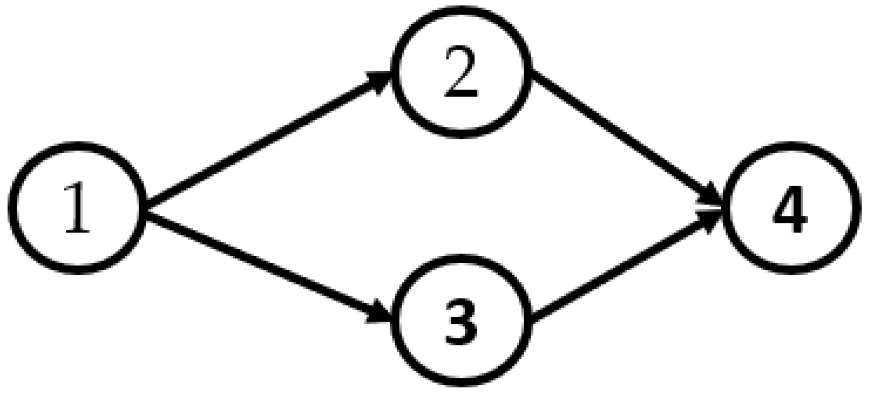
As an example: Suppose the assembly precedence matrix is as follows:

$$A{P}_1=\left(\begin{array}{cccc}0& 1& 1& 0\\ 0& 0& 0& 1\\ 0& 0& 0& 1\\ 0& 0& 0& 0\end{array}\right)$$

(6)

From the matrix, we see that $AP[1][2]=1$; so, $v_1\to v_2$. Similarly, $v_1\to v_3,v_2\to v_4,v_3\to v_4$. The assembly sequence diagram is shown in Figure 3. In the figure, 1, 2, 3, and 4 represent Part 1, Part 2, Part 3, and Part 4, respectively.

4.2. Objective Function Establishment

Assembly Sequence Redirection: A higher number of assembly sequence redirections indicates frequent changes in assembly orientation during the process, reducing assembly efficiency and manufacturability.

For an assembly sequence $\left\{P_1,P_2\dots ,P_n\right\}$ that satisfies geometric feasibility, the corresponding assembly directions are $\left\{d_1,d_2\dots ,d_n\right\}$. The function defining assembly sequence reorientation is defined as follows:

$$X(d_i,d_{i+1})=\left\{\begin{array}{ll}1,\hfill & {\mathrm{if} \mathrm{d}}_i\ne {\mathrm{d}}_{i+1}\hfill \\ 0,\hfill & {\mathrm{if} \mathrm{d}}_i{=\mathrm{d}}_{i+1}\hfill \end{array}\right.$$

(7)

$$g_1(x)={\displaystyle \frac{1}{1+{\displaystyle {\sum }_{i=1}^{n-1}X(d_i,d_{i+1})}}}$$

(8)

where n is the total number of parts in the assembly sequence.

Assembly Tool Aggregation: The greater the assembly tool aggregation, the more frequently tool changes are required, resulting in higher assembly time costs.

Given an assembly sequence $\left\{P_1,P_2\dots ,P_n\right\}$, where the corresponding assembly tools are $\left\{t_1,t_2\dots ,t_n\right\}$, the function defining the assembly tool aggregation for the sequence is defined as follows:

$$X(t_i,t_{i+1})=\left\{\begin{array}{ll}1,\hfill & {\mathrm{if} \mathrm{t}}_i\ne {\mathrm{t}}_{i+1}\hfill \\ 0,\hfill & {\mathrm{if} \mathrm{t}}_i{=\mathrm{t}}_{i+1}\hfill \end{array}\right.$$

(9)

$$g_2(x)={\displaystyle \frac{1}{1+{\displaystyle {\sum }_{i=1}^{n-1}X(t_i,t_{i+1})}}}$$

(10)

where n is the total number of parts in the assembly sequence.

Assembly Accuracy Constraint Function: To quantify the impact of error propagation on system accuracy during assembly, we establish an assembly accuracy objective function based on the Monte Carlo simulation results. Through multiple random perturbations of geometric elements along the error propagation path and iterative calculations, statistical characteristic values for assembly accuracy metrics are obtained. The assembly accuracy objective function primarily relies on the mean error and range as key parameters. The mean error reflects the overall precision level of the assembly sequence, while the range characterizes the fluctuation range of the error distribution. The objective function is defined as follows:

$$X(s)=\alpha ·{\mu }^{(s)}+\beta ·(V_{\max }^{(s)}-V_{\min }^{(s)})$$

(11)

$$g_3(x)={\displaystyle \frac{1}{X(s)+1}}$$

(12)

${\mu }^{(s)}$ denotes the mean error of sequence S, $V_{\max }^{(s)}-V_{\min }^{(s)}$ denotes the range, reflecting the fluctuation range of the data, and $\alpha ,\beta$ are weighting coefficients, where $\alpha +\beta =1$. In practical simulations, the mean is more widely applicable, whereas the range is less robust. Based on engineering handbooks and expert recommendations, we select the system default values $\alpha =0.7$ and $\beta =0.3$.

After obtaining the initial assembly sequence, a greedy algorithm is employed to optimize the assembly sequence. During the optimization process, the corresponding solution is selected as the optimal scheme based on the criterion of maximizing the objective function [43]. The objective function F is defined by Equation (13):

$$F=W_1·g_1(x)+W_2·g_2(x)+W_3·g_3(x)$$

(13)

In the formula, $W_1+W_2+W_3=1$, $W_1,W_2\ll W_3$, $W_1,W_2,W_3$ represent the weights corresponding to these three indicators. The specific values of these weights can be determined by process designers or users based on the actual product characteristics. In the simulation software, designers can set these values through a dedicated dialog box; the system default values are W₁= W₂ = 0.2 and W₃= 0.6. This weighting scheme is based on the analytic hierarchy process and engineering experience.

Based on the initial assembly sequence obtained, parallel parts are selected greedily according to the aforementioned objective function. Through this approach, the greedy algorithm makes the optimal choice under the current circumstances at each step. This strategy enables locally optimal selections to eventually accumulate into a globally optimal solution.

4.3. Improved Topological Sorting Algorithm

Traditional assembly sequence planning methods primarily focus on the number of tool changes and changes in assembly direction while neglecting the impact of assembly accuracy. Furthermore, existing assembly sequence algorithms often perform searches across the entire solution space without filtering for feasibility constraints. To address these issues, we propose an improved topological sorting algorithm. The algorithm first generates a set of candidate assembly sequences that satisfy geometric feasibility based on the assembly precedence graph. Building on this, a greedy selection mechanism is introduced: when determining the next assembly part from the set of candidates, the algorithm evaluates the objective function for each candidate part. Specifically, for each candidate part, the algorithm constructs a hypothetical sequence using the currently determined prefix of the assembly sequence as the next assembly part and then applies the assembly accuracy prediction model described in Section 3 to perform a Monte Carlo simulation on this hypothetical sequence, calculating its mean error and range. These accuracy metrics, together with the number of tool changes and direction changes, form the objective function used to evaluate the relative merits of the candidate parts. Through this mechanism, assembly accuracy is directly incorporated into every decision step of the greedy selection process, thereby achieving accuracy-oriented sequence planning.

Before performing a Monte Carlo simulation on the hypothetical sequence using the assembly accuracy prediction model described in Section 3, symmetric parts are first identified within the set of candidate assembly sequences. This identification is based on the bounding box information of the parts: if the bounding box dimensions of two parts are identical and their projections on each coordinate axis plane overlap, the two parts are deemed to be symmetric. Symmetric parts are treated as a “super-node” and combined into a single representation within the candidate set. This identification process effectively reduces the search space, eliminates redundant sequences caused by the permutation of symmetric parts, and provides a more streamlined and representative candidate set for subsequent greedy selection.

The comprehensive algorithm proceeds as follows:

• After assembly interference detection, obtain the assembly priority relationship matrix to construct the assembly priority relationship model. Generate an assembly priority diagram.
• Initialize a temporary set T to store components without preceding dependencies. These dependencies are derived from the assembly priority graph.
• Greedily select a component from T, remove it from the assembly drawing, and simultaneously delete all directed links originating from that component.
• After completing the topological sorting of all nodes, output the optimal assembly sequence.

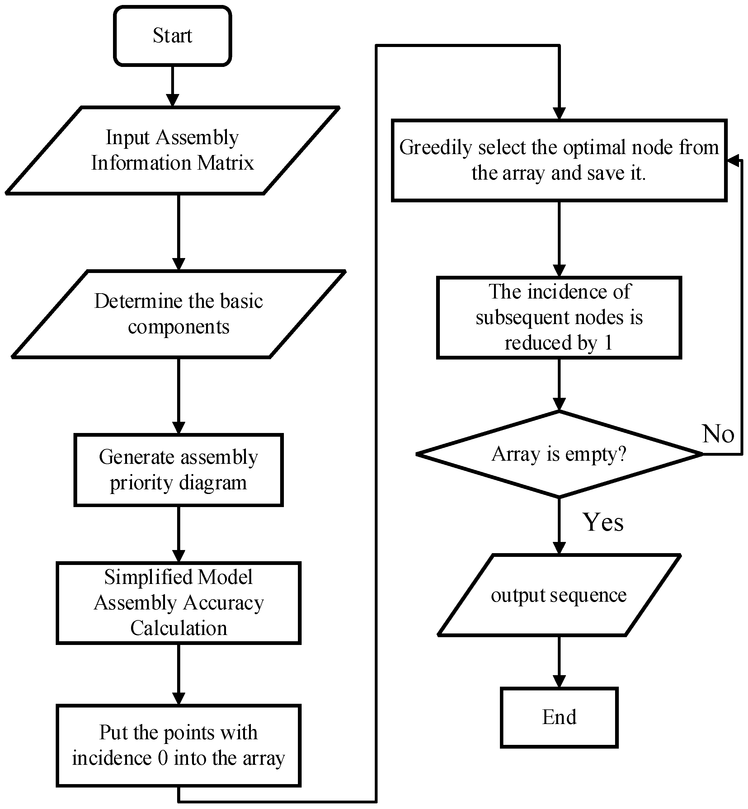
To clearly illustrate the execution logic of this algorithm, we have visualized this using flowcharts and pseudocode. Figure 4 shows the overall flow and control structure of the algorithm, while Algorithm 3 provides specific operational details for each step. Let TS be an array representing a temporary sequence used to store vertices that currently have no direct predecessors (i.e., vertices with in-degree zero).

Algorithm 3. Improving the topological sorting algorithm.

Input: Adjacency matrix of the priority graph, AP.

Output: The excellent sequence, ES.

1: // Search the vertex without immediate predecessor in AP.

2: for i = 1 to n do

3:    if i without immediate predecessor then

4:        TS store i;

5:    end if

6: end for

7: // Sequence from TS and extend TS.

8: while TS ≠ ∅ do

9:      Select j from TS with greedy strategy;

10:       TM store the immediate successor of j;

11:       Delete j and each arc in AP;

12:       if The vertex in TM without immediate predecessor then

13:          TS store it;

14:     end if

15: end while

The assembly precedence graph shown in Figure 3 is topologically sorted, yielding the following result: {1, (2, 3), 4}. We assume that the objective function values for the $<1,2>$ sequence are $g_1=0.15, g_2=0.2, g_3=0.3$, $F_{1\to 2}=0.25$, and those for the $<1,3>$ sequence are $g_1=0.2, g_2=0.1, g_3=0.6$, $F_{1\to 3}=0.42$. Since 0.42 > 0.25, the greedy selection results in part 3; thus, the assembly sequence is 1→3→2→4.

5. Comprehensive Evaluation Indicators for Assembly Sequences

Assembly sequence evaluation is an indispensable key component of assembly sequence planning, and its results directly reflect the quality of the planning algorithm’s solution. We propose a comprehensive evaluation method that takes into account both part-level and product-level metrics.

5.1. Component-Level Evaluation Metrics

The weight of the parts is a key factor affecting the complexity and efficiency of assembly operations. Generally speaking, components that are too light are difficult to position stably during assembly and are prone to slipping or shifting, often requiring the use of precision clamping tools for assistance; conversely, components that are too heavy place higher demands on handling, positioning, and control of assembly orientation, typically necessitating the use of lifting equipment or specialized fixtures. Both of these situations increase the time required for each assembly operation to varying degrees, thereby affecting overall assembly efficiency. The standard for determining this value is given by Equation (14):

$$z_1(x)=\left\{\begin{array}{ll}0\hfill & x<a\hfill \\ {\displaystyle \frac{x-a}{b-a}}\hfill & \mathrm{a}\le \mathrm{x}\le \mathrm{b}\hfill \\ 1\hfill & \mathrm{b}\le \mathrm{x}\le \mathrm{c}\hfill \\ {\displaystyle \frac{d-x}{d-c}}\hfill & \mathrm{c}\le \mathrm{x}\le \mathrm{d}\hfill \\ 0\hfill & \mathrm{x}>d\hfill \end{array}\right.$$

(14)

In the formula, a represents the minimum weight of a part that can be handled manually without specialized handling tools, and d represents the maximum handling weight under the corresponding conditions; handling efficiency is optimal when the part’s mass falls within the range of b to c. The closer the value of the evaluation function is to 1, the shorter the assembly time required for that part. We focus on the actual handling conditions of workers on the shop floor and determine the values of a, b, c, and d to be 10 g, 2.5 kg, 7.5 kg, and 15 kg, respectively.

The number of reference points for a part is one of the key indicators used to measure its structural importance within an assembly; it is defined as the frequency with which a given part serves as a mounting reference point for other parts during the assembly process. The standard for determining this value is given by Equation (15):

$$z_2(x)={\displaystyle \frac{1}{1+e^{-\mathrm{x}}}}$$

(15)

where x represents the number of times it provides assembly support points for other components.

There are significant differences in structural stability among various types of connections after assembly. Among four typical connection types, welded connections offer the highest structural stability because they form a permanent, non-detachable joint and are assigned the highest rating of 1; threaded connections achieve fastening through a threaded pair, offering high connection strength and detachability, and are assigned a rating of 0.8; shaft-hole connections rely on mating surfaces to transmit loads, offering the next highest stability, with a rating of 0.6; and contact connections rely solely on surface contact to maintain relative position, with no additional fastening measures, and thus have the lowest structural stability, with a rating of 0.4. The standard for determining this value is given by Equation (16):

$$z_3(x)=\left\{\begin{array}{ll}0\hfill & \mathrm{contact} \mathrm{connection}\hfill \\ 0.4\hfill & \mathrm{shaft} \mathrm{connection}\hfill \\ 0.7\hfill & \mathrm{screw} \mathrm{connection}\hfill \\ 1\hfill & \mathrm{soldered}\hfill \end{array}\right.$$

(16)

5.2. Product-Level Evaluation Metrics

Number of assembly orientation changes: Changes in orientation often require repositioning and recalibration. The standard for determining this value is given by Equation (17):

$$e_1(x)={\displaystyle \frac{1}{X(d)+1}}$$

(17)

where X(d) represents the number of times the assembly direction has changed.

Number of tool changes: Although tool change operations do not directly contribute to part assembly, they consume additional cycle time due to a series of auxiliary actions—such as picking up the tool, adjusting its orientation, and placing it—and these non-value-added operations significantly increase the time cost of each assembly cycle. The standard for determining this value is given by Equation (18):

$$e_2(x)={\displaystyle \frac{1}{X(t)+1}}$$

(18)

where X(t) represents the number of tool changes

Assembly accuracy: Assembly accuracy quantifies the cumulative effect of errors during the assembly process and directly impacts product functionality; therefore, it is a key metric for evaluating the quality of an assembly solution. The standard for determining this value is given by Equation (19):

$$e_3(x)=\left\{\begin{array}{ll}0\hfill & \Delta (S)>{\Delta }_{\max }\hfill \\ 1-{\displaystyle \frac{\Delta (S)}{{\Delta }_{\max }}}\hfill & 0<\Delta (S)<{\Delta }_{\max }\hfill \end{array}\right.$$

(19)

$\Delta (S)$: The mean error of the simulated statistics for this accuracy characteristic under assembly sequence S, the maximum permissible deviation during the design phase, is ${\Delta }_{\max }$.

In summary, the evaluation metric is given by Equation (20):

$$E=w_1 {\displaystyle {\sum }_{i=1}^3{z}_i(x)}+w_2 {\displaystyle {\sum }_{j=1}^3{e}_j(x)}$$

(20)

In the formula, $w_1+w_2=1$, $w_1,w_2$ represents the weights assigned to these two indicators.

6. Simulation Software Development

Based on the above research, we present a simulation software for assembly sequence planning that integrates assembly accuracy calculations. The software comprises two core modules: the assembly sequence planning module and the assembly accuracy calculation module. Developed on the MFC platform using the C++ programming language, the software leverages the Inte3D platform and SOLIDWORKS for secondary development and supports the import of mainstream CAD file formats (such as models exported from SOLIDWORKS and Inte3D). All experimental simulations were performed on a hardware platform configured with an Intel Core i7-10700F @ 2.90 GHz and 32 GB of RAM.

In particular, the assembly sequence planning software, developed on the Inte3D platform, provides features such as interference detection, automatic extraction of assembly information matrices, modeling of assembly precedence relationships, assembly sequence planning, and the generation of simulation animations. The assembly accuracy simulation module integrates automatic reading of component dimensional information, automatic search for dimensional chains, and automatic construction of accuracy models. It supports multiple assembly accuracy calculation methods, including the extremum method and Monte Carlo method, and features assembly pass rate statistics.

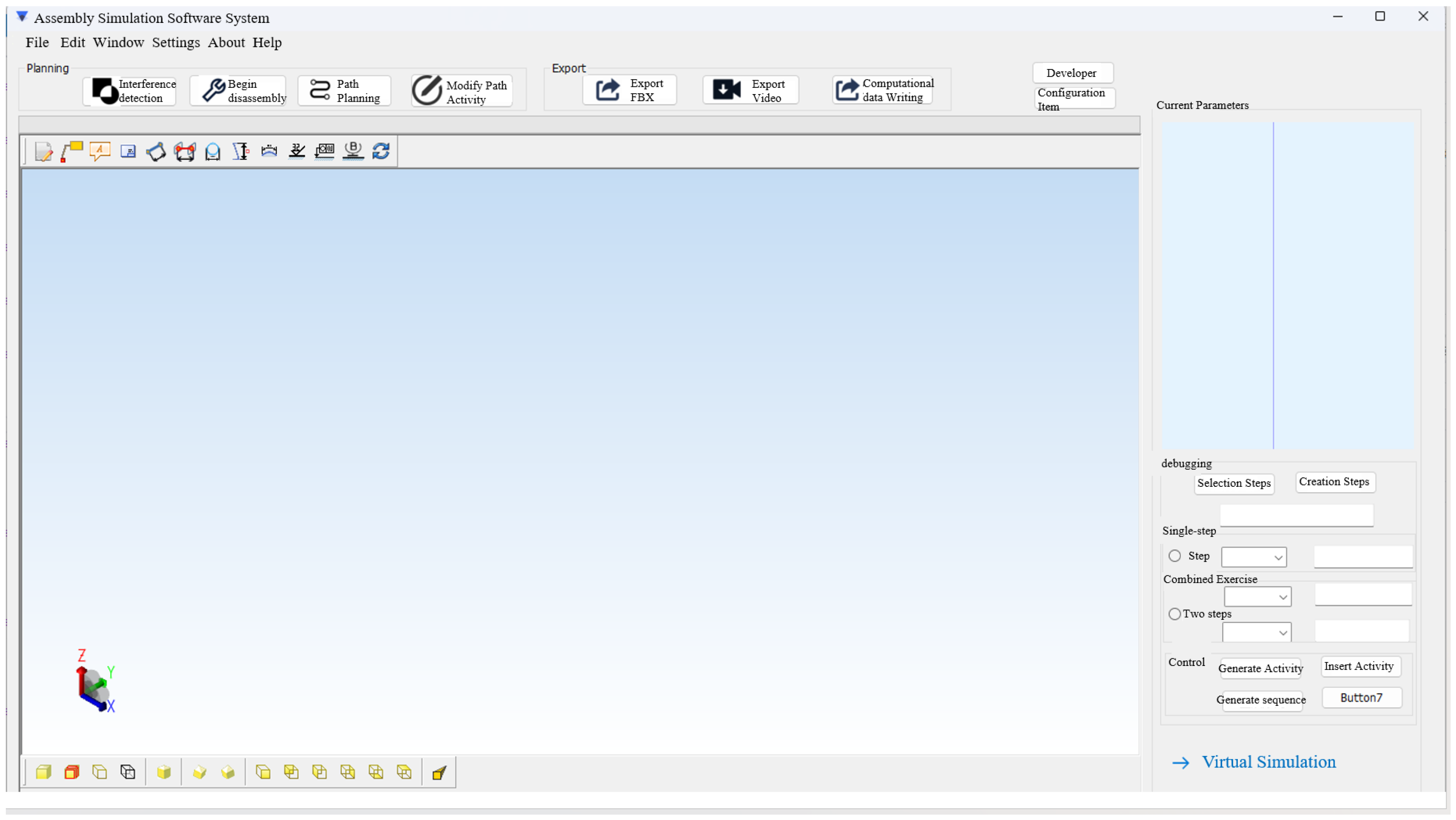
The assembly sequence planning module interface comprises a functional area and an information display. Its initial system operation interface is shown in Figure 5.

The top section of the interface is the functional area, integrating the core modules for assembly sequence planning. These include interference detection, disassembly planning, path planning, path correction, and motion simulation. Additionally, the program offers data export and simulation video generation capabilities, enabling visual presentation of assembly results. The core of the interference check function determines whether parts overlap based on their bounding boxes. After traversing all parts, it generates an interference matrix, connection matrix, and support matrix and displays a pop-up window indicating program completion. If interference exists between parts during program execution, the parts are highlighted for notification.

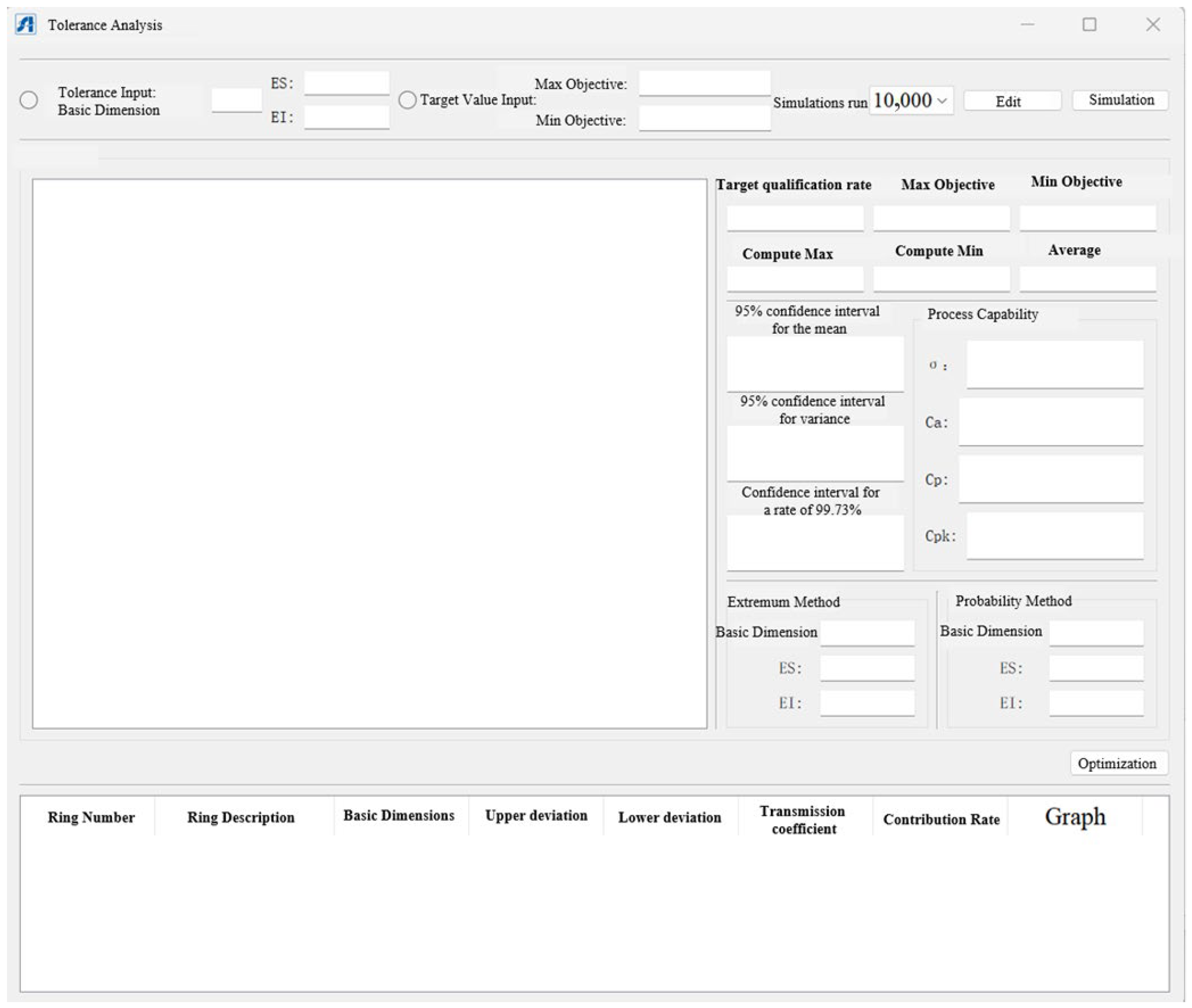
The assembly accuracy simulation module includes a control bar and a calculation result display bar, as shown in Figure 6 below.

The control bar primarily includes functions for tolerance input, target value input, simulation iteration selection, loading assembly file information, and simulation calculation. Click the edit button to select the assembly information file for analysis. The calculation results display panel shows statistical outcomes and distribution histograms following Monte Carlo simulations. This graph automatically labels maximum and minimum values, while the statistics panel displays target maximum, target minimum, calculated maximum, calculated minimum, mean, and the assembly accuracy distribution band under corresponding confidence intervals.

7. Test Results

To comprehensively validate the effectiveness and engineering applicability of the proposed method, this study employs a validation strategy that combines physical verification of typical components with simulation comparisons of complex components. First, using a simplified product model with representative error accumulation characteristics, we verify the physical consistency of the mathematical model for accuracy prediction based on experimental data. Subsequently, we extend this model to complex assemblies with multiple parts and constraints to compare the performance differences among various optimization algorithms.

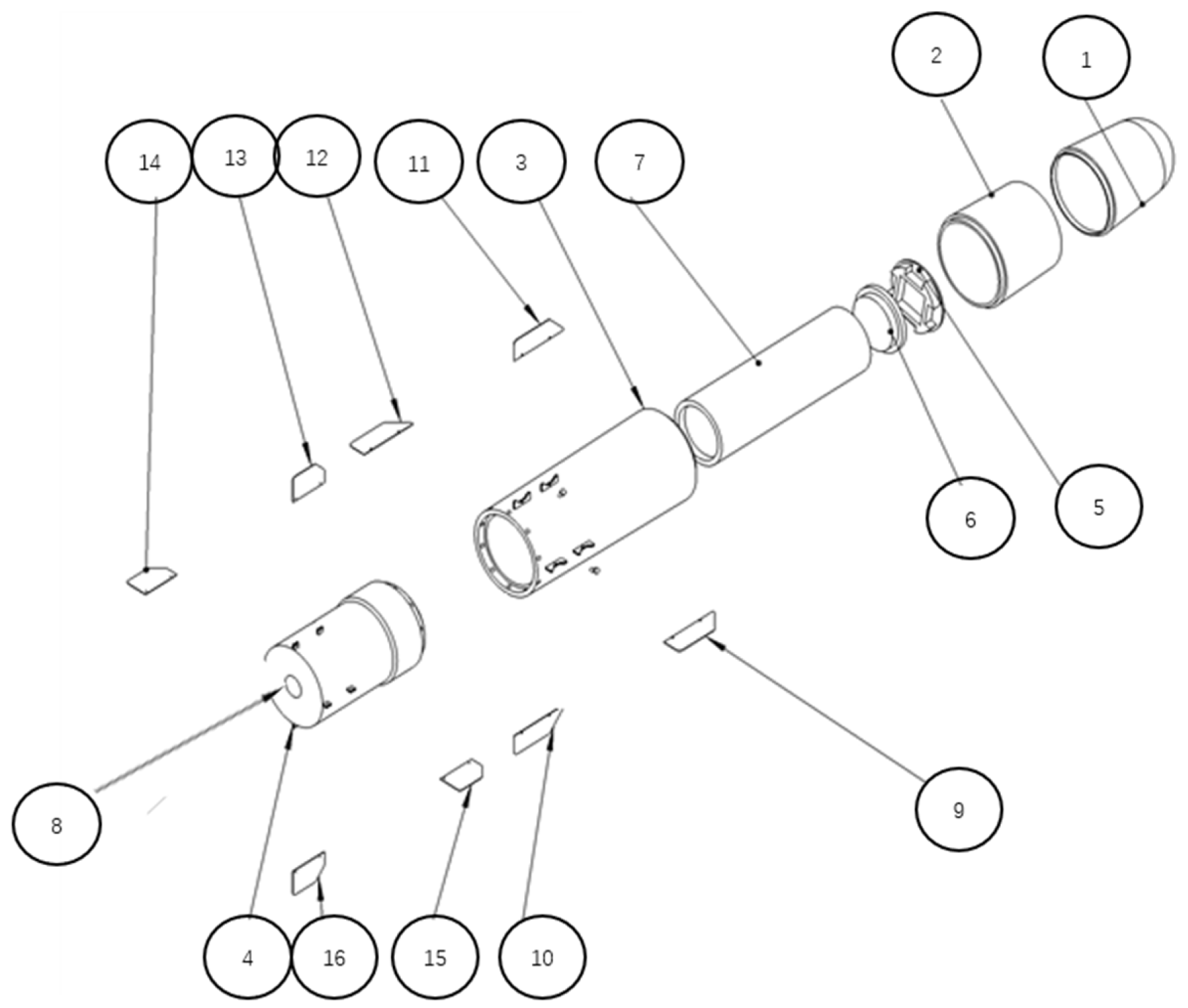
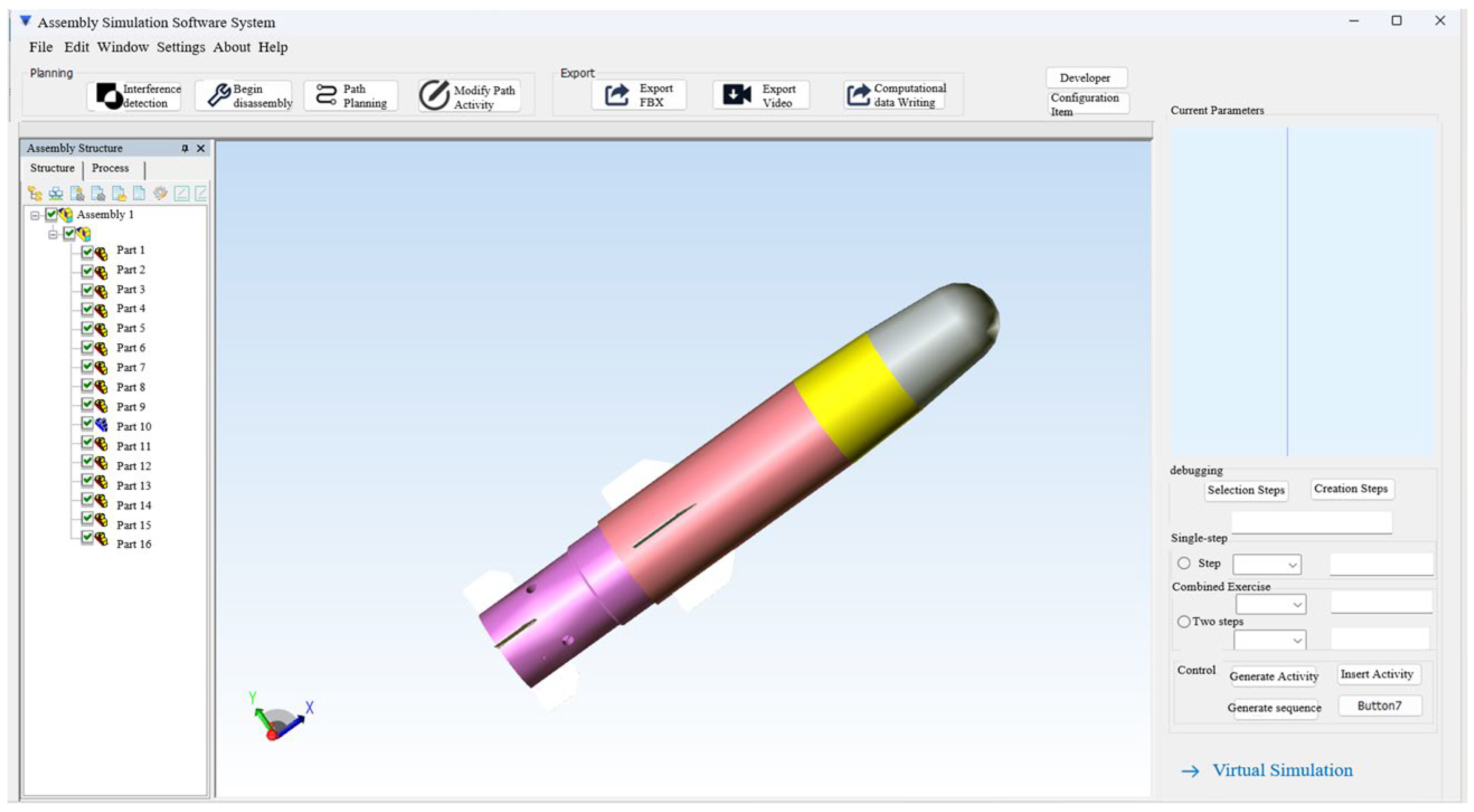
Taking the model shown in Figure 7 as an example, after importing the assembly into the assembly sequence planning and simulation system, the system automatically identifies and reads the quantity and names of each part within the assembly, as shown in Figure 8.

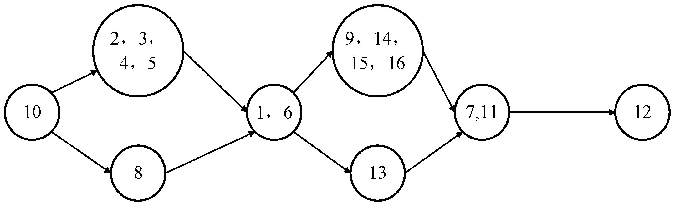
Subsequently, an interference check was performed on the assembly, with the program generating an assembly information matrix in the background. Based on the inspection results, the support matrix and connection matrix were further calculated, thereby identifying the base component as Part 10. Utilizing the assembly priority relationship model established in Section 2, the assembly relationship matrix was converted into an assembly priority graph, with its simplified result shown in Figure 9.

By performing a topological sort based on the assembly precedence graph, the system systematically traverses all nodes in the graph and generates an assembly sequence that satisfies the geometric constraints according to the precedence relationships between parts. The result is as follows: {10, (2, 3, 4, 5, 8), (1, 6), (9, 13, 14, 15, 16), (7, 11), 12}.

Based on the feasible sequences generated by topological sorting, a greedy selection strategy is introduced to screen for the optimal sequence. The weight coefficients of the objective function are set as W₁ = W₂ = 0.2, W₃ = 0.6, where W₁ represents the weight for assembly sequence redirectability, W₂ represents the weight for assembly tool aggregation, and W₃ represents the weight for assembly accuracy. By performing a weighted evaluation of the candidate sequences, the sequence with the optimal objective function value is selected as the final assembly sequence. The optimal assembly sequence obtained after the greedy selection is shown below: 10 → 8 → 2 → 3 → 4 → 5 → 1 → 6 → 13 → 14 → 15 → 16 → 9 → 7 → 11 → 12.

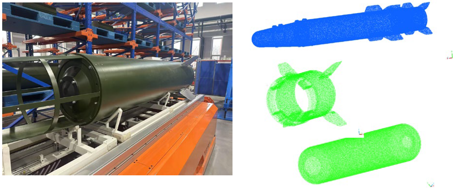
To validate the effectiveness of the simulation method, we used the MetraSCAN 3D point cloud scanner manufactured by CREAFORM to obtain the actual measured dimensions of each section of the assembly and the final assembly. Based on these measurements, we calculated the assembly accuracy for the corresponding assembly sequence and compared it with the simulation results. The product installation and point cloud scanning are shown in Figure 10; the actual point cloud scan values are listed in

Table 2. Point cloud measured values.

Tolerance Type	Actual Measurement (mm)
t1	0.0126
t2	0.3869
t3	0.1273
t4	0.2375
${\Phi }_1$	540.2309
${\Phi }_2$	2351.1864
${\Phi }_3$	553.1163
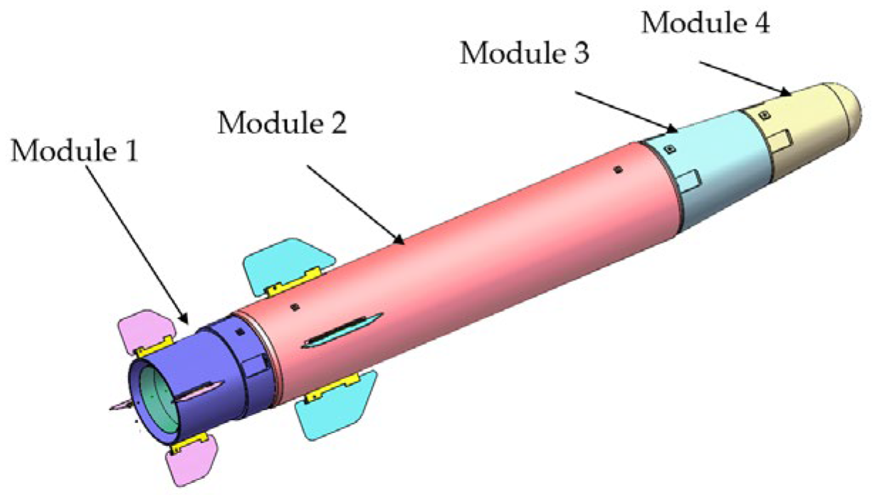
${\Phi }_4$	732.3825

; the compartment division of the model is shown in Figure 11; and the three-dimensional dimensions of the model are listed in

Table 3. The model’s three-dimensional dimensions.

Tolerance Type	Tolerance (mm)
t1	0.05
t2	0.05
t3	0.05
t4	0.05
${\Phi }_1$	${540}_{-0.5}^{+0.5}$
${\Phi }_2$	${2352}_{-0.5}^{+0.5}$
${\Phi }_3$	${552.93}_{-0.5}^{+0.5}$
${\Phi }_4$	${732}_{-0.3}^{+0.5}$

. Specifically, the parallelism error of the reference surface of Module 1 is t₁, the parallelism error of the reference surface of Module 2 is t₂, the perpendicularity error of the centerline of Module 2 is t₃, the parallelism error of the positioning surface for Section 3 is t₄, and the height dimensional tolerances for Modules 1, 2, 3, and 4 are ${\Phi }_1,{\Phi }_2,{\Phi }_3,{\Phi }_4$, respectively.

We calculated the assembly accuracy for the corresponding assembly sequence. The simulation-derived assembly accuracy is 15.7832, while the assembly accuracy calculated from the point cloud-based measured model is 16.1336. Comparing the simulation results with the measured data reveals an error rate of 2.22%, indicating that the simulation results from the proposed method align well with the measured values. The experimental results demonstrate that the proposed assembly accuracy prediction model effectively captures the influence of part tolerances on assembly outcomes.

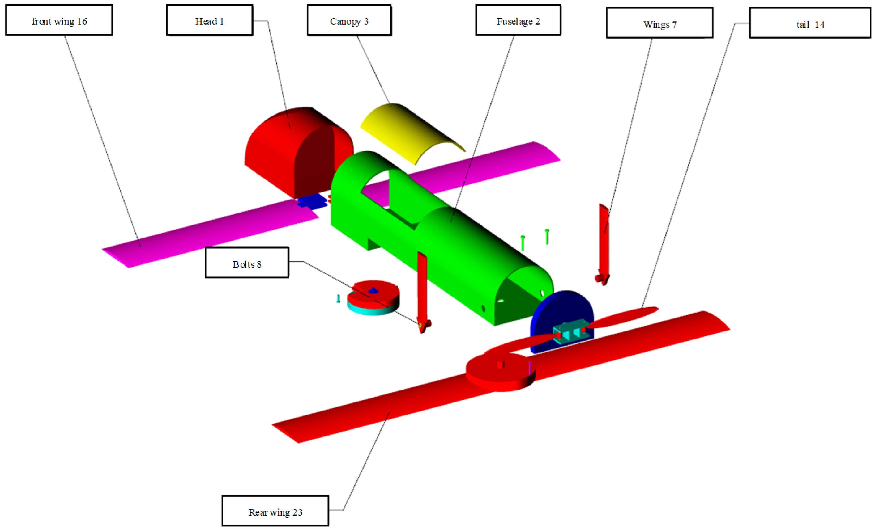
To conduct a comparative analysis of assembly sequences, this study designed a set of control experiments: the first employs a discrete particle swarm algorithm to perform a global search across the entire solution space; the second uses a topological sorting algorithm that optimizes only the number of tool changes and changes in assembly direction, without considering assembly accuracy; and the third group adopted the proposed improved topological sorting algorithm, which takes into account geometric constraints, assembly efficiency, and assembly accuracy. The number of iterations was set to 40. The UAV model shown in Figure 12 serves as the subject of this study. This assembly contains 25 parts.

1—nose, 2—fuselage, 3—upper cover plate, 4—rear cover plate, 5—engine, 6—left wing, 7—right wing, 8—bolt, 9—bolt, 10—bracket, 11—retaining pin, 12—bolt, 13—bolt, 14—left tail wing, 15—right tail wing, 16—left front wing, 17—right front wing, 18—mounting bracket, 19—mounting bracket, 20—bracket, 21—right front wing bracket, 22—front wing shaft, 23—rear wing, 24—retaining pin, and 25—right front wing retaining pin.

After optimization using the discrete particle swarm optimization (DPSO) algorithm, the optimal sequence of this assembly obtained via the DPSO algorithm is as follows: 2 → 5 → 4 → 10 → 6 → 15 → 8 → 16 → 18 → 20 → 21 → 7 → 17 → 9 → 14 → 19 → 13 → 12 → 3 → 25 → 23 → 24 → 22 → 11 → 1.

The topological sorting algorithm, which uses only the number of tool changes and changes in assembly direction as optimization objectives, yields the following assembly sequence: 2 → 5 → 4 → 10 → 6 → 8 → 15 → 16 → 18 → 7 → 20 → 21 → 9 → 14 → 17 → 19 → 3 → 12 → 13 → 11 → 22 → 23 → 24 → 25 → 1.

The assembly sequence obtained using the improved topological sorting algorithm is as follows: 2 → 5 → 4 → 10 → 6 → 8 → 15 → 18 → 16 → 7 → 20 → 21 → 9 → 14 → 17 → 19 → 13 → 12 → 3 → 11 → 22 → 23 → 24 → 25 → 1.

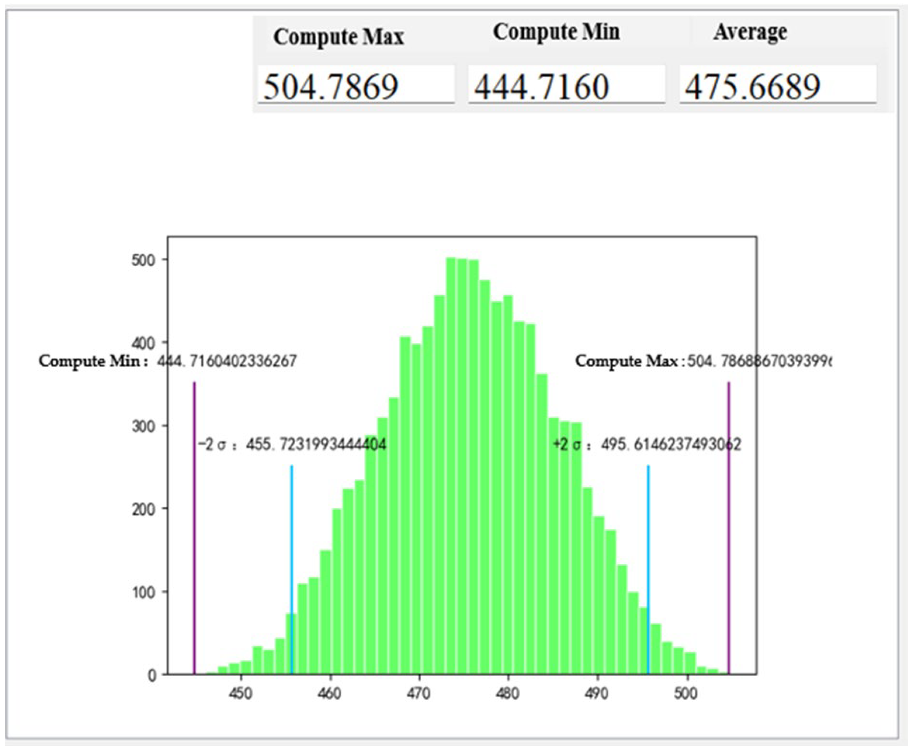
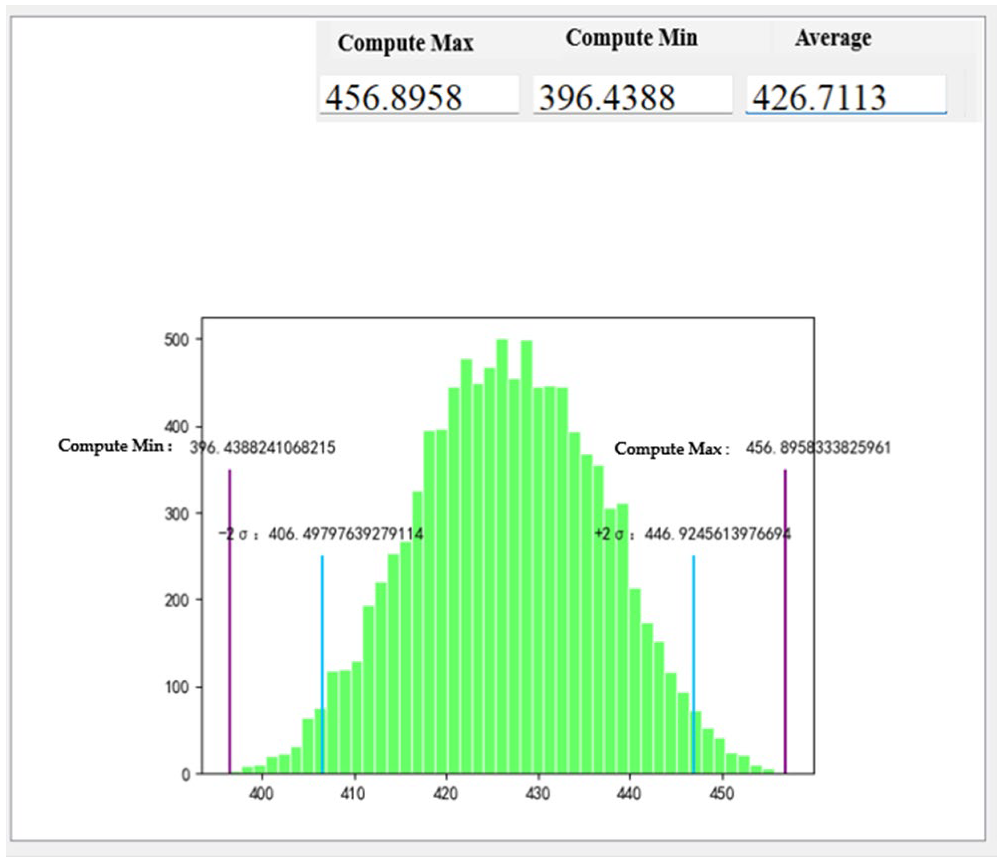
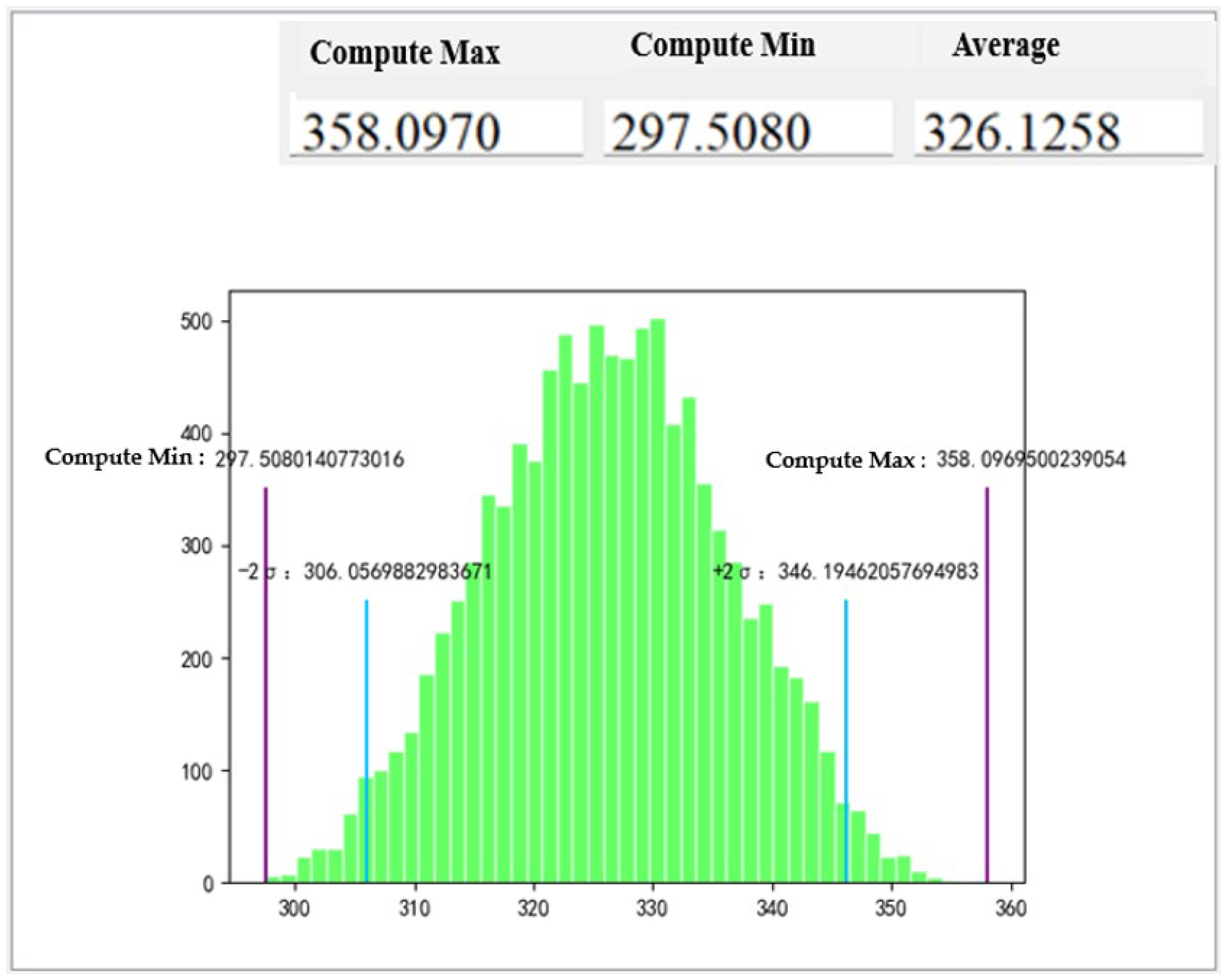
Based on the results of the above analysis, the three assembly sequences were imported into the assembly accuracy simulation system for calculation. Monte Carlo simulation was employed with 10,000 iterations to obtain assembly accuracy simulation results corresponding to the assembly sequence solved by the discrete particle swarm optimization (DPSO) algorithm, the traditional topological sorting sequence that does not consider assembly accuracy, and the assembly accuracy simulation results corresponding to the improved topological sorting algorithm, which takes into account various constraints, including geometric constraints, assembly efficiency constraints, and accuracy constraints. The simulation results are shown in the figure below. The maximum and minimum values represent the upper and lower bounds of the error across 10,000 simulation runs, respectively, and characterize the full range of variation in assembly error for this simulation. These are marked by purple vertical lines in the figure. The mean is the arithmetic mean of all observed sample values, and the green bar chart is a frequency histogram, where the horizontal axis represents the error values and the vertical axis represents the number of samples falling within each interval. The blue vertical lines indicate the 95% confidence interval results. The unit is micrometers. Figure 13 shows the simulation results for assembly accuracy when the assembly sequence is solved using DPSO. As shown in the figure, the upper bound of the error is 504.7869, the lower bound is 444.7160, and the mean error is 475.6689. The 95% confidence interval is [455.7232, 495.6146]. Figure 14 shows the simulation results for assembly accuracy when the assembly sequence is solved using a traditional topological sorting algorithm. As shown in the figure, the upper bound of the error is 456.8958, the lower bound is 396.4388, and the mean error is 426.7113. The 95% confidence interval is [406.4980, 446.9246]. Figure 15 shows the assembly accuracy simulation results corresponding to the improved topological sorting algorithm. As shown in the figure, the upper bound of the error is 358.0970, the lower bound is 297.5080, and the mean error is 326.1258. The 95% confidence interval is [306.0570, 346.1946]. For a detailed comparison and summary of the results, see

Table 4. Comparison of analysis results.

	Maximum Value	Minimum Value	Mean Value
DPSO	504.7869	447.7610	475.6689
Traditional methods	456.8958	396.4388	426.7113
Precision considerations	358.0970	2977.0980	326.1258

.

Table 4 provides a detailed comparison of the solution sequences generated by the DPSO algorithm, which performs a global search over the entire solution space; the efficiency-optimized sequences generated by the traditional topological sorting algorithm; and the accuracy–priority sequence generated by the improved topological sorting algorithm, which takes into account multiple constraints, including geometric constraints, assembly efficiency constraints, and accuracy constraints. The comparison results indicate that the proposed method exhibits better convergence. The improved topological sorting algorithm performs best in terms of error control. Its mean error of 326.1258 is approximately 23.6% lower than that of the traditional topological sorting algorithm and approximately 31.4% lower than that of the DPSO algorithm. This demonstrates that the improved topological sorting algorithm achieves a significant improvement in assembly accuracy. Comparing the numerical ranges in Figure 13, Figure 14 and Figure 15 reveals that the upper bound of the error for the improved algorithm (358.0970) is even lower than the lower bounds of the other two algorithms, and the error distribution has shifted to the left overall. This indicates that the improved algorithm effectively suppresses the accumulation of errors during the assembly process by optimizing the logical relationships in the assembly sequence.

The three algorithms each generated an assembly sequence, which were compared using the comprehensive evaluation metrics described in Section 5. The results are shown in

Table 5. Comparison of solution quality across algorithms.

	Component-Level Evaluation Metrics	Product-Level Evaluation Metrics	Comprehensive Evaluation Indicators	Running Time (s)
DPSO	0.12	0.535	0.655	306.24
Traditional methods	0.13	0.547	0.677	186.58
Precision considerations	0.13	0.748	0.878	223.58

.

Table 5 provides a comparison of the results of the three algorithms in terms of computational efficiency, part level, product level, and comprehensive evaluation metrics. The minimal difference in component-level scores indicates that, under geometric feasibility constraints, the local operability of each sequence is comparable. Product-level scores exhibit a distinct gradient: the proposed algorithm achieves approximately 39.8% higher scores than DPSO and approximately 36.7% higher scores than traditional topological sorting. This validates that, by incorporating an assembly accuracy prediction mechanism, the sequence can effectively avoid paths with high error propagation and improve assembly quality. The overall evaluation metric for DPSO is E₁ = 0.655, while that for the topological sorting algorithm is E₂ = 0.677. The selected algorithm yields a result of E₃ = 0.878. The proposed method achieves better evaluation metrics than the other two methods, demonstrating superior assembly performance. In terms of computational efficiency, the runtime of the proposed algorithm is approximately 27.0% shorter than that of DPSO and approximately 19.8% longer than that of the traditional method. However, the improvement in accuracy far outweighs this trade-off. Overall, the proposed algorithm achieves a significant leap in product-level assembly accuracy at an acceptable cost in terms of computational efficiency.

8. Conclusions

We address the issues of post hoc evaluation of accuracy in assembly sequence planning, the lack of feasibility pruning in search algorithms, and insufficient software integration. We propose a drive-based planning method that integrates assembly accuracy prediction into the sequence generation process. During the modeling of assembly precedence relationships, real-world operational constraints are introduced, and disassembly verification is incorporated to avoid isolated parts with no contact, thereby ensuring the physical feasibility of the sequence from the outset. Building on this foundation, the method actively suppresses tolerance accumulation during sequence generation through assembly priority graph constraints, an improved greedy topological sorting algorithm, and a strategy for merging symmetric parts. Additionally, a one-click virtual assembly simulation system was developed, integrating interference detection, information extraction, sequence planning, simulation animation, and accuracy calculation. This approach generates an optimal sequence that simultaneously balances geometric feasibility, assembly efficiency, and assembly accuracy.

To validate the effectiveness of the proposed method, this study conducted comparative experiments using a specific 3D model. The results indicate that compared to traditional methods optimized solely based on tool change frequency and assembly orientation, the assembly sequences generated by this method demonstrate significantly superior predicted accuracy values and exhibit a narrower range of data fluctuation. This reflects enhanced stability and consistency in the assembly process. Experiments demonstrate that this method effectively enhances assembly precision pass rates while maintaining assembly efficiency, thereby reducing the risk of rework and repair caused by insufficient precision. The core value of this research lies in shifting assembly precision prediction from “post-event verification” to “pre-event optimization,” providing a more practically valuable engineering solution for high-precision assembly sequence planning.

Current assembly accuracy analysis relies heavily on the geometric dimensions, tolerance information, and assembly constraints contained in 3D models. However, in actual engineering practice, models often suffer from missing or incomplete information, making it difficult to establish error propagation diagrams and thereby affecting the accuracy and reliability of accuracy predictions. In the future, it may be worthwhile introducing knowledge graph technology to structurally represent and model the relationships among product structural information, tolerance specifications, historical process data, and domain expert knowledge, thereby constructing a domain-specific knowledge graph tailored for assembly accuracy analysis. Building on this foundation, the semantic reasoning and completion capabilities of the knowledge graph can be leveraged to achieve intelligent matching of missing dimensional information and automatic construction of tolerance chains. This will enhance the completeness and accuracy of error propagation modeling, thereby providing higher-quality data support for assembly accuracy prediction.