PINN-LSTM: A High-Precision Physics-Informed Neural Network for Solving Malware Propagation Dynamics in Wireless Sensor Networks

Abstract

This paper proposes a hybrid PINN + LSTM framework for the high-precision solution of malware propagation dynamics in wireless sensor networks. A seven-compartment SVEHLQR model is developed to capture this complex transmission process. To overcome the limitations of standard physics-informed neural networks (PINNs) in long-term prediction, including gradient vanishing and error accumulation, we integrate LSTM’s temporal memory capability into the PINN architecture. Comprehensive comparisons are conducted among the proposed PINN + LSTM, standard PINN, and Fourier PINN, using the fourth-order Runge–Kutta method as the benchmark. Experimental results demonstrate that PINN + LSTM significantly outperforms both baseline methods, achieving an average relative error of $3.88\times {10}^{-3}$ compared to $7.20\times {10}^{-2}$ for PINN and $2.81\times {10}^{-1}$ for Fourier PINN, representing a 94.6% accuracy improvement over PINN. These results validate that incorporating LSTM’s recursive memory mechanism enables the accurate and efficient solution of complex time-dependent dynamical systems. Additionally, the model’s robustness is verified under 1%, 5%, and 10% Gaussian noise. PINN + LSTM maintains extremely low relative errors, not exceeding 0.0049, and outperforms PINN and Fourier PINN significantly, confirming its strong noise immunity and stable dynamics learning ability in realistic environments.

1. Introduction

In recent years, physics-informed neural networks (PINNs) have emerged as a powerful paradigm for solving differential equations by embedding physical laws directly into the learning process [1,2,3]. The core idea of PINNs is to incorporate governing equations as soft constraints into the loss function via automatic differentiation, which computes derivatives of network outputs with respect to inputs [4,5]. This allows for the construction of residual terms equivalent to the original differential equations, enabling the network to learn system dynamics solely by satisfying physical laws, even in the absence of labeled data. Unlike traditional numerical methods such as finite difference or finite element methods, PINNs are mesh-free, thus avoiding the computational bottlenecks associated with grid generation and the curse of dimensionality. They naturally handle high-dimensional problems, complex boundary conditions, and sparse observational data while integrating data-driven insights with physical knowledge. This makes PINNs particularly advantageous in inverse problems, parameter identification, and uncertainty quantification [6,7]. PINNs have been successfully applied in various fields, including fluid mechanics, solid mechanics, heat transfer, and quantum mechanics.

As a key application area, PINNs have been employed to solve various systems of differential equations derived from epidemiological and propagation models [8,9,10]. Their ability to simultaneously fit observational data while respecting underlying physical laws makes them particularly attractive for modeling complex dynamical systems. Moreover, as these epidemiological and propagation models become increasingly high-dimensional, efficiently solving the resulting differential equation systems poses a critical challenge. Traditional numerical methods such as Runge–Kutta [11], while accurate, incur substantial computational costs and face difficulties in real-time scenarios. However, despite their success across multiple domains, conventional PINNs treat time as an independent spatial dimension and compute derivatives solely through automatic differentiation. This approach introduces two fundamental limitations when solving time-dependent dynamical systems: accumulated errors over long time horizons and the vanishing or exploding gradient problem in deep networks.

To overcome these limitations, this work integrates PINNs with long short-term memory networks. The memory cells and gating mechanisms of LSTM effectively capture long-term dependencies and time-delayed effects, which standard PINNs fail to exploit due to their independent treatment of time points [12,13]. Moreover, the gating structure alleviates gradient vanishing and explosion, stabilizing training and accelerating convergence, making the hybrid PINN + LSTM framework particularly suitable for long-range sequence prediction.

As a concrete application, we consider the problem of malware propagation in wireless sensor networks (WSNs), where accurate modeling and prediction are critical for network security. Malware poses severe threats to WSN stability, causing resource theft, data tampering, and service outages [14]. Given the analogy between malware spread and infectious disease transmission, compartmental models such as SIR and SEIR have been widely adopted to characterize propagation dynamics [15]. However, with increasingly refined node state divisions, the resulting differential equation models become high-dimensional, making efficient solution a critical challenge.

In this paper, we propose a novel PINN + LSTM hybrid model to characterize malware propagation in WSNs. Departing from traditional numerical methods, we employ physics-informed neural networks integrated with long short-term memory to solve the underlying differential equation systems. Using the fourth-order Runge–Kutta (RK4) method as the benchmark, we conduct comprehensive numerical comparisons between the proposed PINN + LSTM, standard PINN, and Fourier PINN. The rest of the paper is organized as follows. Section 2 constructs a malware propagation model based on SEIR epidemic theory. Section 3 introduces the PINN + LSTM framework. Section 4 carries out numerical simulations and a corresponding analysis. Finally, Section 5 concludes the paper and discusses future work.

2. Malware Propagation Model Formulation

In this section, we construct an extended SEIR-based epidemic model with seven state variables, namely Susceptible (S), Vaccinated (V), Exposed (E), High-Risk Infectious (H), Low-Risk Infectious (L), Quarantined (Q), and Recovered (R). Let $S\left(t\right)$, $V\left(t\right)$, $E\left(t\right)$, $H\left(t\right)$, $L\left(t\right)$, $Q\left(t\right)$, and $R\left(t\right)$ denote the density of nodes in each compartment at time t, respectively. We assume that the total number of nodes in the WSNs remains constant over time. Therefore,

$$S\left(t\right)+V\left(t\right)+E\left(t\right)+H\left(t\right)+L\left(t\right)+Q\left(t\right)+R\left(t\right)=1.$$

(1)

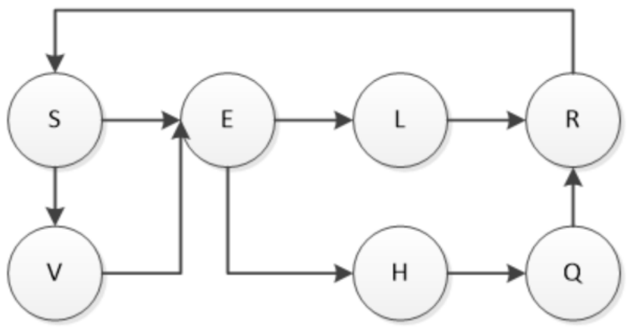
Let $[t,t+\mathrm{\Delta }t]$ be a time interval, where $\mathrm{\Delta }t\ge 0$ is a sufficiently small time segment starting from time t. Based on epidemic theory, the state transition relationships of nodes among different compartments are illustrated in Figure 1.

The density variation in compartment S consists of three components. First, susceptible nodes are protected by the defense system and transition to the vaccinated compartment V at a rate $ϵ$. Second, susceptible nodes can be infected by high-risk and low-risk infectious nodes, and then move to the exposed compartment E at rates ${\alpha }_1$ and ${\alpha }_2$, respectively. Third, some recovered nodes return to the susceptible state at rate $\gamma$. Accordingly, the density change in S over the time interval $[t,t+\mathrm{\Delta }t]$ is formulated as follows:

$$S(t+\mathrm{\Delta }t)-S\left(t\right)=\left(-ϵS\left(t\right)-S\left(t\right)\left({\alpha }_{1}H\left(t\right)+{\alpha }_{2}L\left(t\right)\right)+\gamma R\left(t\right)\right)\mathrm{\Delta }t$$

(2)

The density variation in compartment V consists of two components. First, susceptible nodes are protected by the defense system and transition to the vaccinated compartment V at rate $ϵ$. Second, some vaccinated nodes may still be infected by high-risk and low-risk infectious nodes, and transfer to the exposed compartment E at rates ${\alpha }_3$ and ${\alpha }_4$, respectively, where ${\alpha }_3<{\alpha }_1$ and ${\alpha }_4<{\alpha }_2$. Accordingly, the density change in V over the time interval $[t,t+\mathrm{\Delta }t]$ is formulated as follows:

$$V(t+\mathrm{\Delta }t)-V\left(t\right)=\left(ϵS\left(t\right)-V\left(t\right)({\alpha }_{3}H\left(t\right)+{\alpha }_{4}L\left(t\right))\right)\mathrm{\Delta }t$$

(3)

The density variation in compartment E consists of two components: susceptible and vaccinated nodes can be infected and transition to compartment E (consistent with the infection mechanisms of S and V), and the exposed nodes then progress to compartments H and L at rates ${\beta }_1$ and ${\beta }_2$, respectively. Accordingly, the density change in E over the time interval $[t,t+\mathrm{\Delta }t]$ is formulated as follows:

$$E(t+\mathrm{\Delta }t)-E\left(t\right)=(S\left(t\right)({\alpha }_{1}H\left(t\right)+{\alpha }_{2}L\left(t\right))+V\left(t\right)({\alpha }_{3}H\left(t\right)+{\alpha }_{4}L\left(t\right))-({\beta }_1+{\beta }_2)E\left(t\right))\mathrm{\Delta }t$$

(4)

The density variation in compartment H consists of two components: exposed nodes transfer to compartment H at rate ${\beta }_1$, and high-risk infectious nodes move to compartment Q at rate $\delta$. Accordingly, the density change in H over the time interval $[t,t+\mathrm{\Delta }t]$ is formulated as follows:

$$H(t+\mathrm{\Delta }t)-H\left(t\right)=({\beta }_{1}E\left(t\right)-\delta H\left(t\right))\mathrm{\Delta }t$$

(5)

The density variation in compartment L consists of two components: exposed nodes transition to compartment L at rate ${\beta }_2$, and low-risk infectious nodes recover at rate $\eta$. Accordingly, the density change in L over the time interval $[t,t+\mathrm{\Delta }t]$ is formulated as follows:

$$L(t+\mathrm{\Delta }t)-L\left(t\right)=({\beta }_{2}E\left(t\right)-\eta L\left(t\right))\mathrm{\Delta }t$$

(6)

The density variation in compartment Q is determined by two components: high-risk infectious nodes move to compartment Q at rate $\delta$, and quarantined nodes recover at rate $\eta$. Accordingly, the density change in Q over the time interval $[t,t+\mathrm{\Delta }t]$ is formulated as follows:

$$Q(t+\mathrm{\Delta }t)-Q\left(t\right)=\left(\delta H\right(t)-\eta Q(t\left)\right)\mathrm{\Delta }t$$

(7)

Since the total number of nodes in the WSN is constant, the density variation in compartment R consists of three components: low-risk infectious nodes recover at rate $\eta$, quarantined nodes recover at rate $\eta$, and some recovered nodes return to the susceptible state at rate $\gamma$. Accordingly, the density change in R over the time interval $[t,t+\mathrm{\Delta }t]$ is formulated as follows:

$$R(t+\mathrm{\Delta }t)-R\left(t\right)=\left(\eta \right(Q\left(t\right)+L\left(t\right))-\gamma R(t\left)\right)\mathrm{\Delta }t$$

(8)

We assume that the number of nodes in each state varies continuously within $\mathrm{\Delta }t$. Equations (2)–(8) are in discrete-time difference form; by dividing by $\mathrm{\Delta }t$ and letting $\mathrm{\Delta }t\to 0$, the continuous-time ordinary differential Equation (9) is directly obtained.

$$\left\{\begin{array}{c}{\displaystyle \frac{dS\left(t\right)}{dt}}=-ϵS\left(t\right)-S\left(t\right)({\alpha }_{1}H\left(t\right)+{\alpha }_{2}L\left(t\right))+\gamma R\left(t\right),\hfill \\ {\displaystyle \frac{dV\left(t\right)}{dt}}=ϵS\left(t\right)-V\left(t\right)({\alpha }_{3}H\left(t\right)+{\alpha }_{4}L\left(t\right)),\hfill \\ {\displaystyle \frac{dE\left(t\right)}{dt}}=({\alpha }_{1}S\left(t\right)+{\alpha }_{3}V\left(t\right))H\left(t\right)+({\alpha }_{2}S\left(t\right)+{\alpha }_{4}V\left(t\right))L\left(t\right)-({\beta }_1+{\beta }_2)E\left(t\right),\hfill \\ {\displaystyle \frac{dH\left(t\right)}{dt}}={\beta }_{1}E\left(t\right)-\delta H\left(t\right),\hfill \\ {\displaystyle \frac{dL\left(t\right)}{dt}}={\beta }_{2}E\left(t\right)-\eta L\left(t\right),\hfill \\ {\displaystyle \frac{dQ\left(t\right)}{dt}}=\delta H\left(t\right)-\eta Q\left(t\right),\hfill \\ {\displaystyle \frac{dR\left(t\right)}{dt}}=\eta (Q\left(t\right)+L\left(t\right))-\gamma R\left(t\right),\hfill \end{array}\right.$$

(9)

where the initial condition is $\left\{S\right(0)\ge 0,V(0)\ge 0,E(0)\ge 0,H(0)\ge 0,L(0)\ge 0,Q(0)\ge 0,$$R\left(0\right)\ge 0\}$.

The added complexity of the SVEHLQR model is justified by its ability to capture WSN-specific features. Distinguishing between high-risk infectious (H) and low-risk infectious (L) nodes reflects differences in node roles and transmission capabilities, which is critical for propagation accuracy [16], unlike the homogeneous infectious classes assumed in [17,18]. Furthermore, the introduction of vaccinated (V) and quarantined (Q) compartments incorporates proactive protection and isolation mechanisms, which are absent in basic models but essential for WSN security [19]. Compared to recent works such as [20,21], our model further subdivides infectious states to better align with the heterogeneous communication patterns observed in WSNs. In contrast to [22], which focuses on detection mechanisms, our work models propagation dynamics using a macroscopic compartmental approach suitable for large-scale WSNs.

For the model to be mathematically meaningful, we examine its steady states and derive a basic reproduction number. Let $X={(S,V,E,H,L,Q,R)}^{\top }$. System (9) can be written as

$${\displaystyle \frac{dX}{dt}}=f\left(X\right),$$

(10)

with f Lipschitz continuous.

At a malware-free steady state, no exposed, infected or quarantined nodes exist. Setting $E=H=L=Q=0$ in (9) and solving yields

$$X_0=(0,1,0,0,0,0,0).$$

(11)

This means the entire population is vaccinated. The derivation is straightforward: the first equation gives $-ϵS+\gamma R=0$; with $R=0$ we get $S=0$. The second equation then holds automatically. Normalization of $S+V+E+H+L+Q+R=1$ forces $V=1$.

Following the next-generation method, we isolate the infected compartments. Let $Y={(E,H,L,Q)}^{\top }$. System (9) becomes

$${\displaystyle \frac{𝜕Y}{𝜕t}}=\mathcal{F}-\mathcal{V},$$

(12)

where

$$\mathcal{F}=\left(\begin{array}{c}({\alpha }_{1}S+{\alpha }_{3}V)H+({\alpha }_{2}S+{\alpha }_{4}V)L\\ 0\\ 0\\ 0\end{array}\right),\mathcal{V}=\left(\begin{array}{c}({\beta }_1+{\beta }_2)E\\ -{\beta }_{1}E+\delta H\\ -{\beta }_{2}E+\eta L\\ -\delta H+\eta Q\end{array}\right).$$

(13)

Let f and v be the Jacobians of $\mathcal{F}$ and $\mathcal{V}$ with respect to Y, evaluated at $X_0$:

$$f={\left.{\displaystyle \frac{𝜕\mathcal{F}}{𝜕Y}}\right|}_{X_0}=\left(\begin{array}{cccc}0& {\alpha }_1{S}^0+{\alpha }_3{V}^0& {\alpha }_2{S}^0+{\alpha }_4{V}^0& 0\\ 0& 0& 0& 0\\ 0& 0& 0& 0\\ 0& 0& 0& 0\end{array}\right)=\left(\begin{array}{cccc}0& {\alpha }_3& {\alpha }_4& 0\\ 0& 0& 0& 0\\ 0& 0& 0& 0\\ 0& 0& 0& 0\end{array}\right),$$

(14)

$$v={\left.{\displaystyle \frac{𝜕\mathcal{V}}{𝜕Y}}\right|}_{X_0}=\left(\begin{array}{cccc}{\beta }_1+{\beta }_2& 0& 0& 0\\ -{\beta }_1& \delta & 0& 0\\ -{\beta }_2& 0& \eta & 0\\ 0& -\delta & 0& \eta \end{array}\right).$$

(15)

Computing $v^{-1}$ gives

$$v^{-1}=\left(\begin{array}{cccc}{\displaystyle \frac{1}{{\beta }_1+{\beta }_2}}& 0& 0& 0\\ {\displaystyle \frac{{\beta }_1}{\delta ({\beta }_1+{\beta }_2)}}& {\displaystyle \frac{1}{\delta }}& 0& 0\\ {\displaystyle \frac{{\beta }_2}{\eta ({\beta }_1+{\beta }_2)}}& 0& {\displaystyle \frac{1}{\eta }}& 0\\ {\displaystyle \frac{{\beta }_1}{\eta ({\beta }_1+{\beta }_2)}}& {\displaystyle \frac{1}{\eta }}& 0& {\displaystyle \frac{1}{\eta }}\end{array}\right).$$

(16)

The next-generation matrix is

$$f{v}^{-1}=\left(\begin{array}{cccc}{\displaystyle \frac{{\alpha }_3{\beta }_1\eta +{\alpha }_4{\beta }_2\delta }{\eta \delta ({\beta }_1+{\beta }_2)}}& {\displaystyle \frac{{\alpha }_3}{\delta }}& {\displaystyle \frac{{\alpha }_4}{\eta }}& 0\\ 0& 0& 0& 0\\ 0& 0& 0& 0\\ 0& 0& 0& 0\end{array}\right).$$

(17)

Hence $R_0$, the spectral radius of $f{v}^{-1}$, equals

$$R_0={\displaystyle \frac{{\alpha }_3{\beta }_1\eta +{\alpha }_4{\beta }_2\delta }{\eta \delta ({\beta }_1+{\beta }_2)}}.$$

(18)

Standard results from epidemic theory tell us that the stability of $X_0$ is governed by $R_0$. When $R_0<1$, the malware-free equilibrium is locally asymptotically stable. In practical terms, a small outbreak will not spread and eventually disappears. When $R_0>1$, $X_0$ loses stability and the malware can invade the population. The case $R_0=1$ marks a transcritical bifurcation where the two equilibria exchange stability.

For $R_0>1$, there exists a nontrivial endemic equilibrium $X^{*}=(S^{*},V^{*},E^{*},H^{*},L^{*},Q^{*},R^{*})$ with $H^{*}>0$. Solving the steady-state equations yields the following relations:

$$\begin{array}{cc}\hfill E^{*}& ={\displaystyle \frac{\delta H^{*}}{{\beta }_1}},\hfill \\ \hfill L^{*}& ={\displaystyle \frac{{\beta }_2\delta H^{*}}{{\beta }_1\eta }},\hfill \\ \hfill Q^{*}& ={\displaystyle \frac{\delta H^{*}}{\eta }},\hfill \\ \hfill R^{*}& ={\displaystyle \frac{({\beta }_1+{\beta }_2)\delta H^{*}}{\gamma {\beta }_1}},\hfill \\ \hfill S^{*}& ={\displaystyle \frac{({\beta }_1+{\beta }_2)\eta \delta H^{*}}{\eta {\beta }_1ϵ+\eta {\beta }_1{\alpha }_1{H}^{*}+{\alpha }_2{\beta }_2\delta H^{*}}},\hfill \\ \hfill V^{*}& ={\displaystyle \frac{ϵS^{*}}{{\alpha }_3{H}^{*}+{\alpha }_4{L}^{*}}}.\hfill \end{array}$$

(19)

Substituting these into $S^{*}+V^{*}+E^{*}+H^{*}+L^{*}+Q^{*}+R^{*}=1$ gives an equation for $H^{*}$. The explicit form is omitted as our focus is numerical rather than analytical.

3. Physics-Informed Neural Network Fused with LSTM Model

In this section, a hybrid physics-informed neural network integrated with long short-term memory (PINN + LSTM) is proposed to solve the numerical solution of the malware propagation system (9) accurately. The traditional fully connected PINN treats time as a static input feature and lacks the ability to capture long-term temporal dependencies in dynamic systems, which easily leads to accumulated errors and non-physical drift in long-time predictions. To address this limitation, the LSTM module is embedded into the PINN framework to enhance the model’s capability of memorizing historical dynamic information and modeling sequential evolution patterns, thereby improving the stability and accuracy of the numerical solution for the malware propagation system.

The PINN + LSTM model inherits the core advantage of PINNs by encoding physical laws into the training process via a physics-informed loss function. Meanwhile, it leverages the LSTM’s recursive memory mechanism to capture the temporal correlation of the dynamic system. The overall architecture of the model consists of four key components: an input layer, a time embedding layer, a stacked LSTM encoder, and a fully connected decoder. The detailed structure and mathematical formulation are presented as follows.

3.1. Network Architecture and Forward Propagation

The input of the PINN + LSTM model is the scalar time variable $t\in [t_0,t_T]$ (where $t_0=0$ is the initial time and $t_T$ is the terminal time), and the output is the predicted value of the 7-dimensional state vector $\widehat{\mathbf{X}}\left(t\right)={[\widehat{S}\left(t\right),\widehat{V}\left(t\right),\widehat{E}\left(t\right),\widehat{H}\left(t\right),\widehat{L}\left(t\right),\widehat{Q}\left(t\right),\widehat{R}\left(t\right)]}^T$, which corresponds exactly to the solution of the malware propagation system given in Equation (9).

The time input t is first mapped to a high-dimensional feature space through the embedding layer to enhance the expressive ability of temporal features. The mathematical formulation of the embedding layer is

$${\mathbf{z}}_t=tanh\left(W_{\mathrm{emb}}·t+b_{\mathrm{emb}}\right)$$

(20)

where ${\mathbf{z}}_t\in {\mathbb{R}}^{d_{\mathrm{emb}}}$ is the embedded time feature vector, $W_{\mathrm{emb}}$ and $b_{\mathrm{emb}}$ are trainable parameters, and $tanh(·)$ is the hyperbolic tangent activation function.

To capture the dynamic evolutionary characteristics of the malware propagation system, an LSTM encoder is introduced to memorize the historical states of $\widehat{S},\widehat{V},\widehat{E},\widehat{H},\widehat{L},\widehat{Q},\widehat{R}$ during temporal propagation. Based on the embedded feature ${\mathbf{z}}_t$, the LSTM updates its internal states through four gate mechanisms, which are mathematically defined as follows:

• Forget Gate (${\mathbf{f}}_t$): Controls the retention of historical dynamic information related to the malware propagation states.

  $${\mathbf{f}}_t=\sigma \left(W_f·[{\mathbf{z}}_t,{\mathbf{h}}_{t-1}]+b_f\right)$$

  (21)

  where $\sigma (·)$ is the sigmoid activation function that constrains gate values between 0 and 1, $W_f$ is the weight matrix of the LSTM gates, ${\mathbf{h}}_{t-1}$ is the hidden state at the previous time step, initialized as ${\mathbf{h}}_0=\mathbf{0}$, and $b_f$ is the bias vector of the LSTM gates.
• Input Gate (${\mathbf{i}}_t$): Regulates the update of new temporal information for the epidemic states.

  $${\mathbf{i}}_t=\sigma \left(W_i·[{\mathbf{z}}_t,{\mathbf{h}}_{t-1}]+b_i\right)$$

  (22)

  where $W_i$ is the weight matrix of the LSTM gates, and $b_i$ is the bias vector of the LSTM gates.
• Cell State Update: Integrates historical memory and new features to maintain continuous evolution of the malware propagation trend.

  $${\tilde{\mathbf{c}}}_t=tanh\left(W_c·[{\mathbf{z}}_t,{\mathbf{h}}_{t-1}]+b_c\right)$$

  (23)

  $${\mathbf{c}}_t={\mathbf{f}}_t\odot {\mathbf{c}}_{t-1}+{\mathbf{i}}_t\odot {\tilde{\mathbf{c}}}_t$$

  (24)

  where ⊙ is the element-wise (Hadamard) product, ${\mathbf{c}}_t\in {\mathbb{R}}^{d_{\mathrm{hid}}}$ is the cell state that maintains long-term memory of state variables $\widehat{S},\widehat{V},\widehat{E},\widehat{H},\widehat{L},\widehat{Q},\widehat{R}$, $W_c$ is the weight matrix of the LSTM gates, $b_c$ is the bias vector of the LSTM gates, and ${\mathbf{c}}_{t-1}$ is the cell states at the previous time step, initialized as ${\mathbf{c}}_0=\mathbf{0}$.
• Output Gate and Hidden State: Outputs temporal features that reflect the evolutionary trend of the malware propagation system.

  $${\mathbf{o}}_t=\sigma \left(W_o·[{\mathbf{z}}_t,{\mathbf{h}}_{t-1}]+b_o\right)$$

  (25)

  $${\mathbf{h}}_t={\mathbf{o}}_t\odot tanh\left({\mathbf{c}}_t\right)$$

  (26)

  where ${\mathbf{h}}_t\in {\mathbb{R}}^{d_{\mathrm{hid}}}$ is the hidden state that records the evolutionary features of the malware propagation system, $W_o$ is the weight matrix of the LSTM gates, and $b_o$ is the bias vector of the LSTM gates.

The decoder is a fully connected PINN-style network that maps the LSTM hidden state ${\mathbf{h}}_t$ to the physical state variables of the malware propagation system. It outputs the predicted solution $\widehat{\mathbf{X}}\left(t\right)$ that satisfies the dynamic constraints of System (9):

$$\begin{array}{cc}\hfill {\mathbf{h}}_{\mathrm{dec}1}& =tanh\left(W_{\mathrm{dec}1}·{\mathbf{h}}_t+b_{\mathrm{dec}1}\right),\hfill \\ \hfill {\mathbf{h}}_{\mathrm{dec}2}& =tanh\left(W_{\mathrm{dec}2}·{\mathbf{h}}_{\mathrm{dec}1}+b_{\mathrm{dec}2}\right),\hfill \\ \hfill \widehat{\mathbf{X}}\left(t\right)& =W_{\mathrm{out}}·{\mathbf{h}}_{\mathrm{dec}2}+b_{\mathrm{out}}.\hfill \end{array}$$

(27)

where ${\mathbf{h}}_{\mathrm{dec}1},{\mathbf{h}}_{\mathrm{dec}2}\in {\mathbb{R}}^{d_{\mathrm{hid}}}$ are the hidden layer features of the decoder, $W_{\mathrm{dec}1},W_{\mathrm{dec}2},W_{\mathrm{out}}$ are the weight matrices, and $b_{\mathrm{dec}1},b_{\mathrm{dec}2},b_{\mathrm{out}}$ are the bias vectors.

By combining LSTM-based temporal memory and PINN-based physical constraints, the PINN + LSTM model accurately learns the dynamic evolution of $\widehat{S},\widehat{V},\widehat{E},\widehat{H},\widehat{L},\widehat{Q},\widehat{R}$ while strictly satisfying the malware propagation ODE system.

3.2. Training Objective and Loss Function

The training of the PINN + LSTM model is guided by a physics-informed loss function, which enforces the model output to satisfy both the initial conditions of the malware propagation system and the dynamic constraints described by the ODEs. The total loss function $Loss$ consists of two components: the initial condition loss $Los{s}_{\mathrm{ic}}$ to ensure consistency with the initial state and the physics-informed residual loss $Los{s}_{\mathrm{f}}$ to enforce compliance with the ODE system, which is formulated as

$$Loss=Los{s}_{\mathrm{ic}}+\lambda ·Los{s}_{\mathrm{f}}$$

(28)

where $\lambda$ is the weight coefficient of the residual loss, used to balance the importance of the initial condition and physical constraints.

The initial condition loss measures the squared error between the model’s predicted output at the initial time $t=0$ and the given initial state values of the malware propagation system. The mathematical formulation is

$$\begin{array}{cc}\hfill Los{s}_{\mathrm{ic}}=& {\left(\widehat{S}\left(0\right)-S_0\right)}^2+{\left(\widehat{V}\left(0\right)-V_0\right)}^2+{\left(\widehat{E}\left(0\right)-E_0\right)}^2+\hfill \\ \hfill & {\left(\widehat{H}\left(0\right)-H_0\right)}^2+{\left(\widehat{L}\left(0\right)-L_0\right)}^2+{\left(\widehat{Q}\left(0\right)-Q_0\right)}^2+{\left(\widehat{R}\left(0\right)-R_0\right)}^2\hfill \end{array}$$

(29)

where $S_0,V_0,E_0,H_0,L_0,Q_0,R_0$ are the given initial values of the seven state variables, which are consistent with the initial conditions of System (9), and $\widehat{S}\left(0\right),\widehat{V}\left(0\right),\dots ,\widehat{R}\left(0\right)$ are the predicted values of the PINN + LSTM model at $t=0$.

The residual loss is the core of the PINN framework, which forces the model output to satisfy the ODE constraints of the malware propagation system. For a set of collocation points ${\left\{t_j\right\}}_{j=1}^l$ (randomly sampled within the time interval $[0,t_T]$, l is the number of collocation points), the residual of each state variable is defined as the difference between the temporal derivative of the model’s predicted value and the corresponding right-hand side of the ODE in System (9).

To obtain the temporal derivatives ${\displaystyle \frac{d\widehat{S}}{dt}},{\displaystyle \frac{d\widehat{V}}{dt}},\dots ,{\displaystyle \frac{d\widehat{R}}{dt}}$ needed for residual evaluation, we apply automatic differentiation. This approach enables accurate and efficient computation of output derivatives with respect to the input time t without manual symbolic derivation.

Although the LSTM layer updates its hidden state ${\mathbf{h}}_t$ recursively from the preceding state ${\mathbf{h}}_{t-1}$, the full network is regarded as a continuous mapping from the scalar input t to the estimated state vector $\widehat{\mathbf{X}}\left(t\right)$. The internal recurrence of the LSTM defines the structure of the approximator rather than a discrete dynamic update, so the network remains differentiable with respect to t.

The derivatives are computed through the chain rule in network backpropagation. The total derivative of the output state $\widehat{\mathbf{X}}\left(t\right)$ with respect to time is expressed as

$${\displaystyle \frac{d\widehat{\mathbf{X}}\left(t\right)}{dt}}={\displaystyle \frac{𝜕\widehat{\mathbf{X}}}{𝜕{\mathbf{h}}_{\mathrm{dec}2}}}·{\displaystyle \frac{𝜕{\mathbf{h}}_{\mathrm{dec}2}}{𝜕{\mathbf{h}}_{\mathrm{dec}1}}}·{\displaystyle \frac{𝜕{\mathbf{h}}_{\mathrm{dec}1}}{𝜕{\mathbf{h}}_t}}·{\displaystyle \frac{𝜕{\mathbf{h}}_t}{𝜕{\mathbf{z}}_t}}·{\displaystyle \frac{𝜕{\mathbf{z}}_t}{𝜕t}},$$

(30)

where each term is evaluated analytically during backpropagation. The term ${\displaystyle \frac{𝜕{\mathbf{h}}_t}{𝜕{\mathbf{z}}_t}}$ naturally captures the recursive update rule ${\mathbf{h}}_t=LSTM({\mathbf{z}}_t,{\mathbf{h}}_{t-1})$ within the LSTM cell. The resulting derivative represents the exact continuous-time gradient of the predicted trajectory, which is mathematically consistent with the derivative required by the ODE residual. This construction is supported by existing research on physics-informed recurrent networks, whose convergence can be guaranteed under mild regularity conditions on the dynamical system.

Based on the automatic differentiation results, the residual functions for each state variable are defined as follows:

$$\left\{\begin{array}{c}\begin{array}{cc}\hfill f_S\left(t_j\right)& ={\displaystyle \frac{d\widehat{S}}{dt}}{|}_{t_j}-\left[-ϵ\widehat{S}\left(t_j\right)-\widehat{S}\left(t_j\right)\left({\alpha }_1\widehat{H}\left(t_j\right)+{\alpha }_2\widehat{L}\left(t_j\right)\right)+\gamma \widehat{R}\left(t_j\right)\right],\hfill \\ \hfill f_V\left(t_j\right)& ={\displaystyle \frac{d\widehat{V}}{dt}}{|}_{t_j}-\left[ϵ\widehat{S}\left(t_j\right)-\widehat{V}\left(t_j\right)\left({\alpha }_3\widehat{H}\left(t_j\right)+{\alpha }_4\widehat{L}\left(t_j\right)\right)\right],\hfill \\ \hfill f_E\left(t_j\right)& ={\displaystyle \frac{d\widehat{E}}{dt}}{|}_{t_j}-\left[\left({\alpha }_1\widehat{S}\left(t_j\right)+{\alpha }_3\widehat{V}\left(t_j\right)\right)\widehat{H}\left(t_j\right)+\left({\alpha }_2\widehat{S}\left(t_j\right)+{\alpha }_4\widehat{V}\left(t_j\right)\right)\widehat{L}\left(t_j\right)-({\beta }_1+{\beta }_2)\widehat{E}\left(t_j\right)\right],\hfill \\ \hfill f_H\left(t_j\right)& ={\displaystyle \frac{d\widehat{H}}{dt}}{|}_{t_j}-\left[{\beta }_1\widehat{E}\left(t_j\right)-\delta \widehat{H}\left(t_j\right)\right],\hfill \\ \hfill f_L\left(t_j\right)& ={\displaystyle \frac{d\widehat{L}}{dt}}{|}_{t_j}-\left[{\beta }_2\widehat{E}\left(t_j\right)-\eta \widehat{L}\left(t_j\right)\right],\hfill \\ \hfill f_Q\left(t_j\right)& ={\displaystyle \frac{d\widehat{Q}}{dt}}{|}_{t_j}-\left[\delta \widehat{H}\left(t_j\right)-\eta \widehat{Q}\left(t_j\right)\right],\hfill \\ \hfill f_R\left(t_j\right)& ={\displaystyle \frac{d\widehat{R}}{dt}}{|}_{t_j}-\left[\eta \left(\widehat{Q}\left(t_j\right)+\widehat{L}\left(t_j\right)\right)-\gamma \widehat{R}\left(t_j\right)\right].\hfill \end{array}\hfill \end{array}\right.$$

(31)

The residual loss is the average of the squared residuals over all collocation points, which quantifies the degree to which the model output violates the ODE constraints:

$$Los{s}_{\mathrm{f}}={\displaystyle \frac{1}{l}}\sum _{j=1}^l\left[f_S^2\left(t_j\right)+f_V^2\left(t_j\right)+f_E^2\left(t_j\right)+f_H^2\left(t_j\right)+f_L^2\left(t_j\right)+f_Q^2\left(t_j\right)+f_R^2\left(t_j\right)\right]$$

(32)

3.3. Model Training Process

The trainable parameters of the PINN + LSTM model include all weight matrices and bias vectors of the embedding layer, LSTM encoder, and decoder:

$$\mathsf{\Theta }=\{W_{\mathrm{emb}},b_{\mathrm{emb}},W_f,b_f,W_i,b_i,W_c,b_c,W_o,b_o,W_{\mathrm{dec}1},b_{\mathrm{dec}1},W_{\mathrm{dec}2},b_{\mathrm{dec}2},W_{\mathrm{out}},b_{\mathrm{out}}\}.$$

The training process aims to minimize the total loss function $Loss$ with respect to $\mathsf{\Theta }$, which is implemented using the Adam optimizer to adjust the parameters iteratively. The learning rate is dynamically adjusted using a learning rate scheduler, which reduces the learning rate by a factor of 0.5 when the loss does not decrease for 500 consecutive epochs, to improve convergence stability.

The training steps are summarized as follows:

• Step 1: Initialize all trainable parameters $\mathsf{\Theta }$ using the Xavier normal initialization method to avoid vanishing/exploding gradients at the start of training;
• Step 2: Randomly sample l collocation points ${\left\{t_j\right\}}_{j=1}^l$ within the time interval $[0,t_T]$;
• Step 3: For each epoch, compute the model output $\widehat{\mathbf{X}}\left(t\right)$ for the collocation points and initial time $t=0$ via forward propagation;
• Step 4: Compute the initial condition loss $Los{s}_{\mathrm{ic}}$ and the residual loss $Los{s}_{\mathrm{f}}$ (using automatic differentiation to compute temporal derivatives);
• Step 5: Compute the total loss $Loss$ and backpropagate the gradient to update the parameters $\mathsf{\Theta }$ using the Adam optimizer;
• Step 6: Repeat steps 2–5 until the loss converges to a stable value or the maximum number of epochs (10,000 epochs in this study) is reached.

Compared with a traditional fully connected PINN, the PINN + LSTM model benefits from the LSTM module in two key aspects: it captures temporal dependencies and remembers historical dynamic information, while achieving more stable long-term prediction with less accumulated error and non-physical drift.

4. Numerical Simulations and Performance Analysis

In this section, a series of numerical simulations is carried out to verify the effectiveness of the proposed PINN + LSTM model for solving the malware propagation dynamic system in a wireless sensor network. All simulations are implemented in Python 3.7. The traditional fully connected PINN [23], the Fourier feature-based PINN, and the proposed PINN + LSTM are comprehensively compared, where the fourth-order Runge–Kutta (RK4) method is used as a high-precision reference solution. The comparison covers training convergence, state variable prediction, multi-dimensional error metrics, long-term stability, and error distribution. All experiments are implemented in PyTorch (1.13.1+cpu) with the same initial conditions, network parameters, and training settings for fairness.

The simulation interval is set to $t\in [0,80]$, with 1500 uniform sampling points for testing and 500 collocation points for training. The parameters of the epidemic dynamics system are given as

$$\begin{array}{cc}& ϵ=0.01,{\alpha }_1=0.025,{\alpha }_2=0.03,{\alpha }_3=0.02,{\alpha }_4=0.015,\hfill \\ & {\beta }_1=0.3,{\beta }_2=0.45,\delta =0.05,\eta =0.08,\gamma =0.04.\hfill \end{array}$$

The initial states of the seven compartments are

$$[S_0,V_0,E_0,H_0,L_0,Q_0,R_0]=[0.5,0.3,0.1,0.1,0.0,0.0,0.0].$$

Both networks are trained for 10,000 epochs using the Adam optimizer with an initial learning rate of ${10}^{-3}$. The PINN uses four hidden layers with 128 neurons per layer. The PINN + LSTM uses an embedding layer, two LSTM layers with 128 hidden units, and a two-layer fully connected decoder. To ensure reproducibility, the penalty coefficient is set to $\lambda =100$ and the random seed is fixed at 42.

4.1. Training Dynamics and Convergence

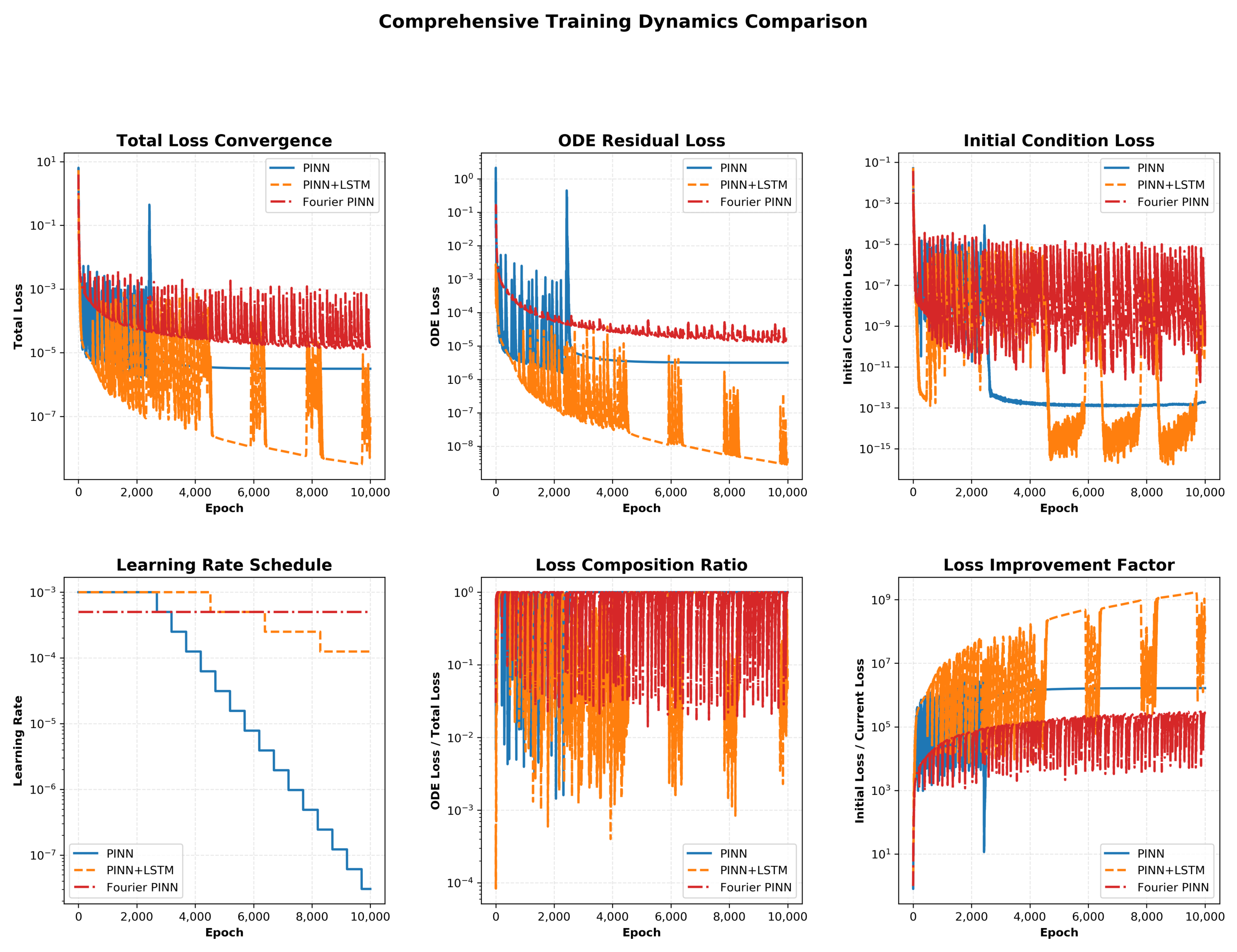
Figure 2 shows the training loss curves of the traditional fully connected PINN, the Fourier feature-based PINN, and the proposed PINN + LSTM, including total loss, ODE residual loss, initial condition loss, and learning rate decay.

A comparative analysis of the training logs reveals distinct performance characteristics among the traditional PINN, the PINN + LSTM model, and the Fourier feature-based PINN for solving differential equations. In terms of convergence speed, the traditional PINN’s total loss fell from an initial 5.18 to a final value of $3.13\times {10}^{-6}$, a reduction of approximately six orders of magnitude. The Fourier PINN’s total loss decreased from 3.94 to $1.39\times {10}^{-5}$, achieving a five-order-of-magnitude reduction. By contrast, the PINN + LSTM model saw its total loss drop from 5.45 to $9.40\times {10}^{-8}$, a reduction of over seven orders of magnitude. This suggests that integrating the LSTM structure notably improves both convergence rate and final approximation accuracy. The PINN + LSTM’s final ODE loss reached $4.34\times {10}^{-9}$, nearly three orders of magnitude lower than that of the traditional PINN and the Fourier PINN.

The PINN + LSTM exhibited a notable loss rebound at epoch 3000, with total loss jumping from $2.49\times {10}^{-7}$ to $3.12\times {10}^{-4}$, signifying temporary instability during training. This phenomenon is attributed to the structural oscillation during optimization, which is a normal behavior when the model balances learning long-term temporal dynamics and satisfying physical constraints, rather than a sign of training failure. Regarding the satisfaction of initial conditions, the traditional PINN achieved an extremely precise IC loss of $1.91\times {10}^{-13}$, followed by the Fourier PINN with $9.20\times {10}^{-11}$, while the PINN + LSTM recorded an IC loss of $8.97\times {10}^{-10}$. In summary, the traditional PINN offers a highly stable training process with excellent adherence to initial conditions. The Fourier PINN delivers moderate performance in both convergence accuracy and stability. In contrast, the PINN + LSTM achieves superior solution accuracy and ODE residual minimization, albeit at the cost of minor training instability, making it better suited for complex dynamical problems where high precision is the top priority.

4.2. State Variable Prediction

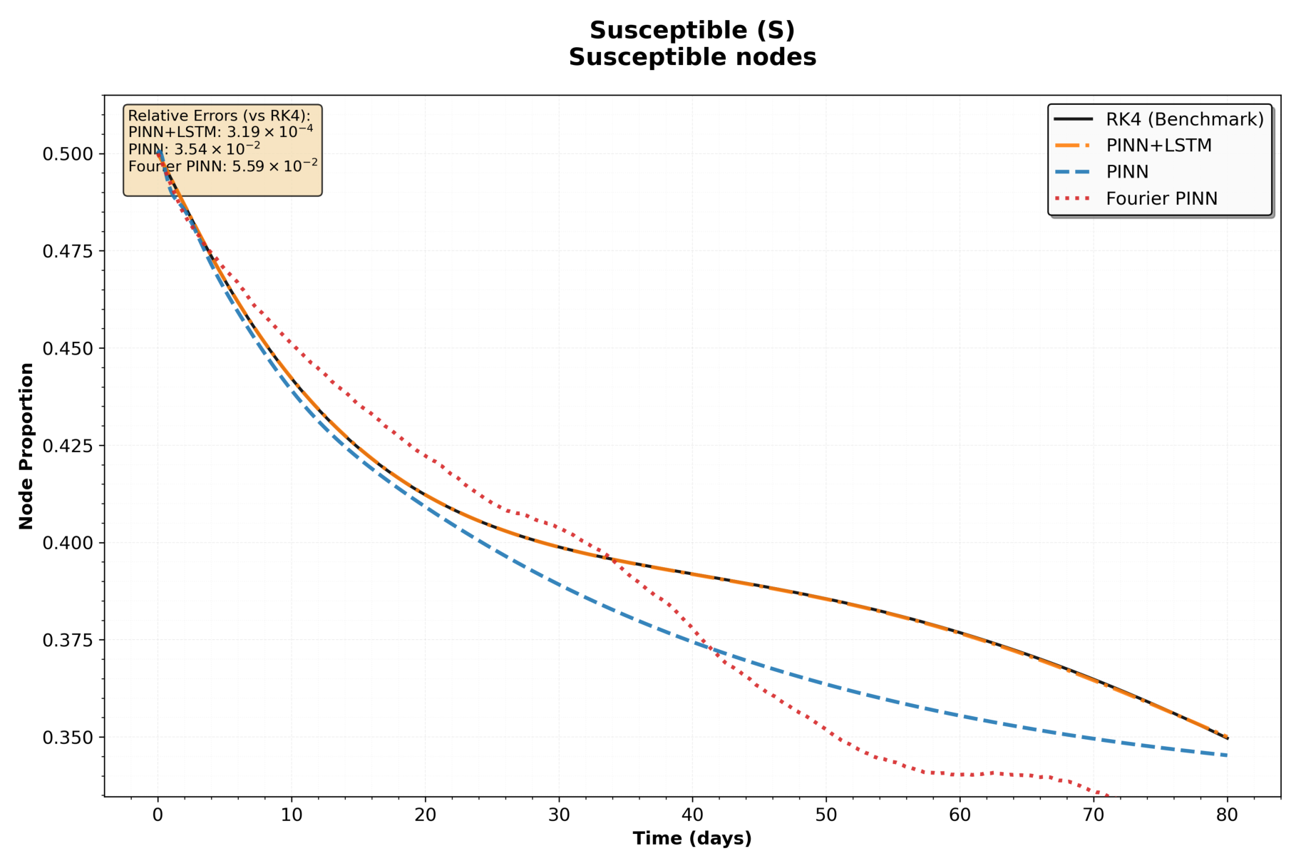
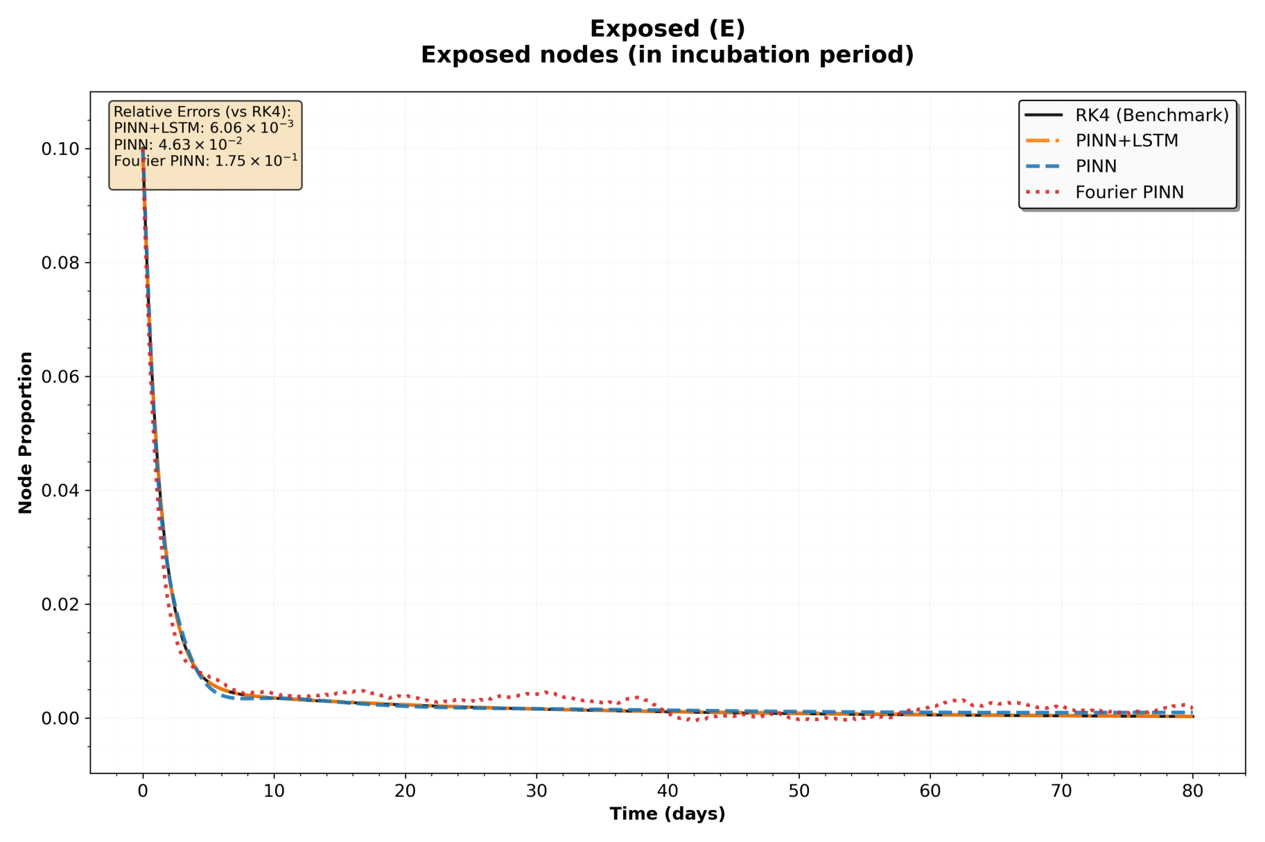
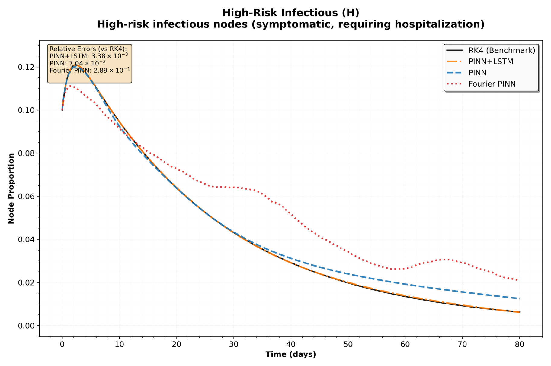
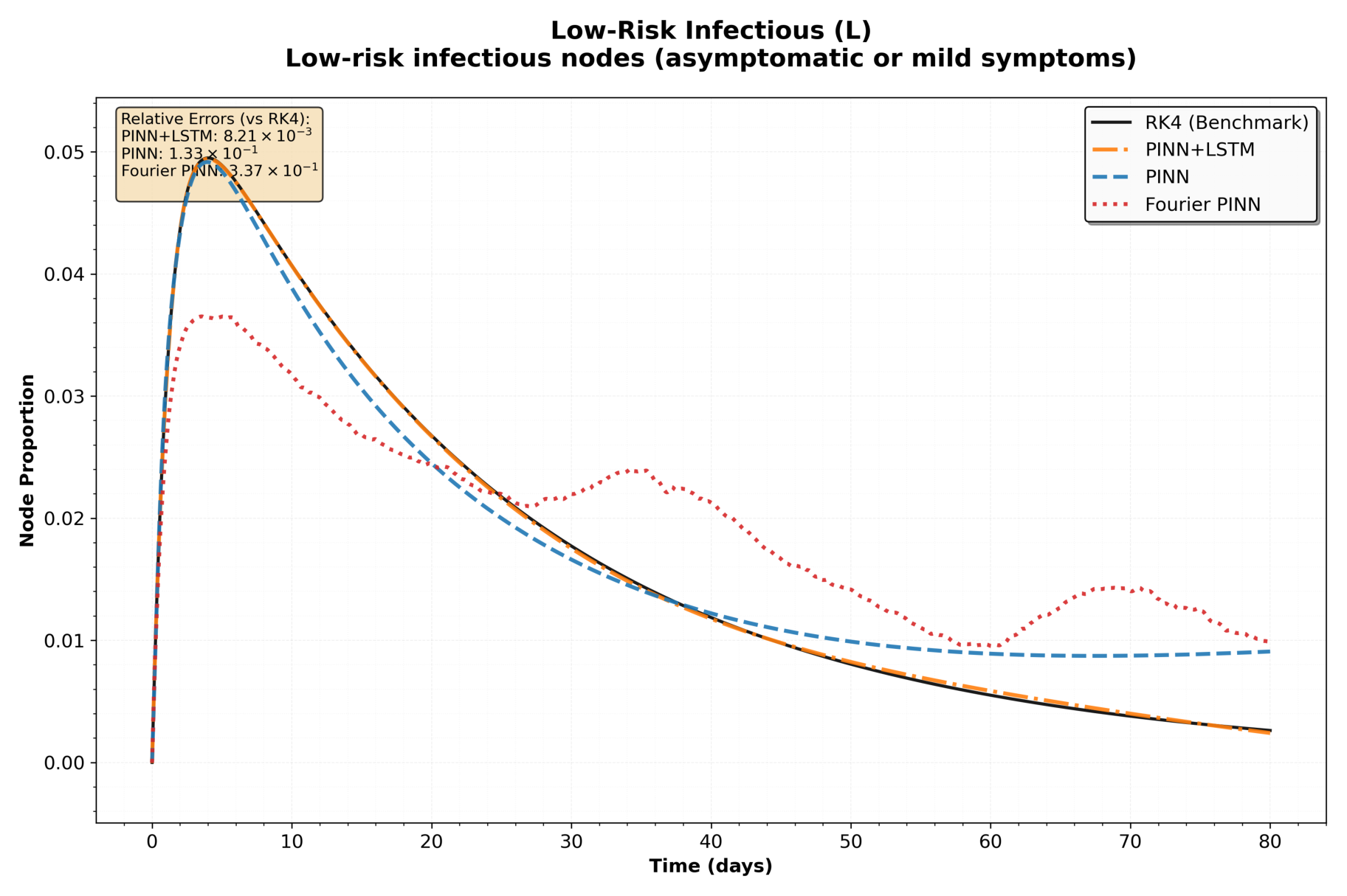
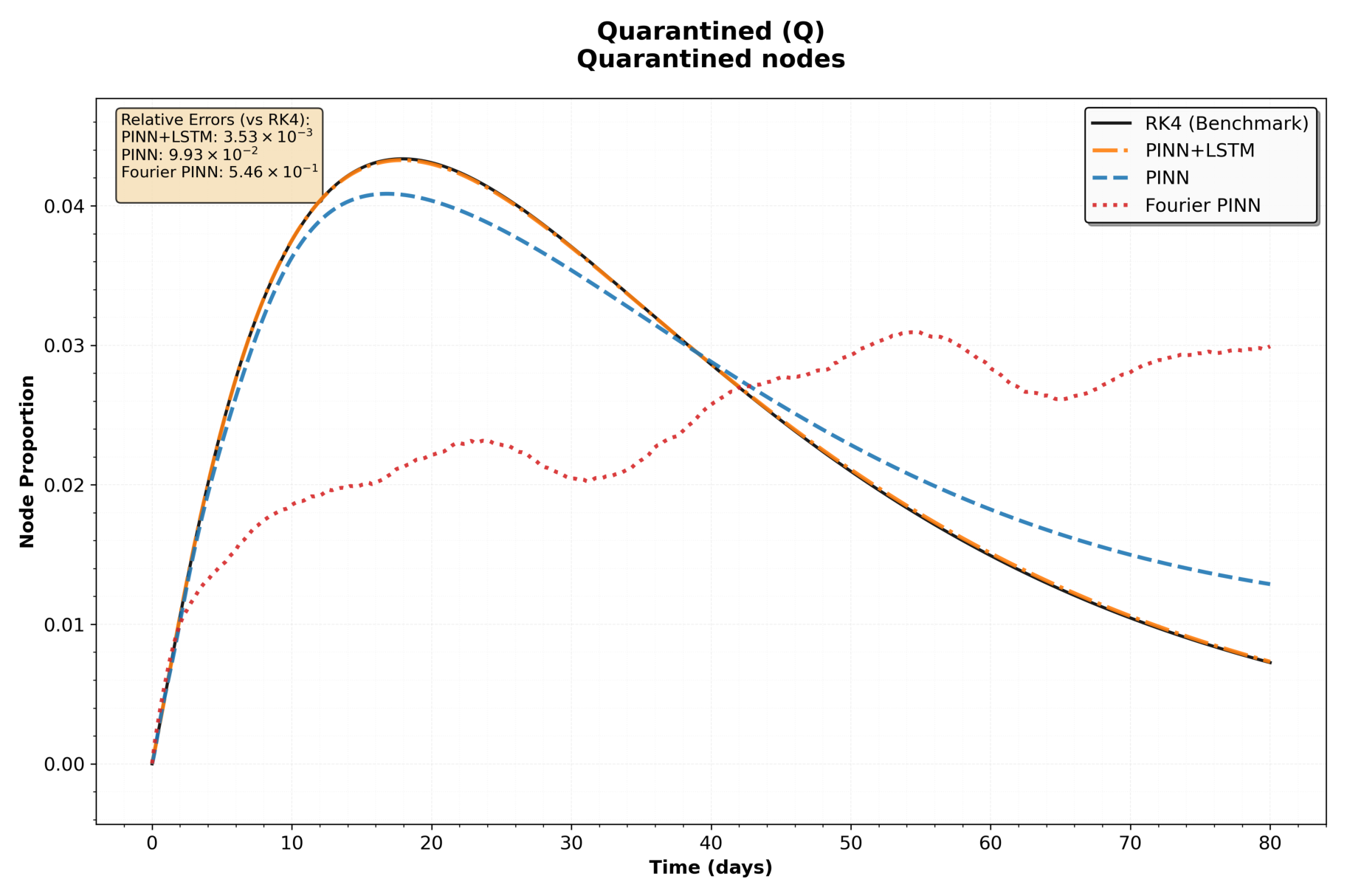
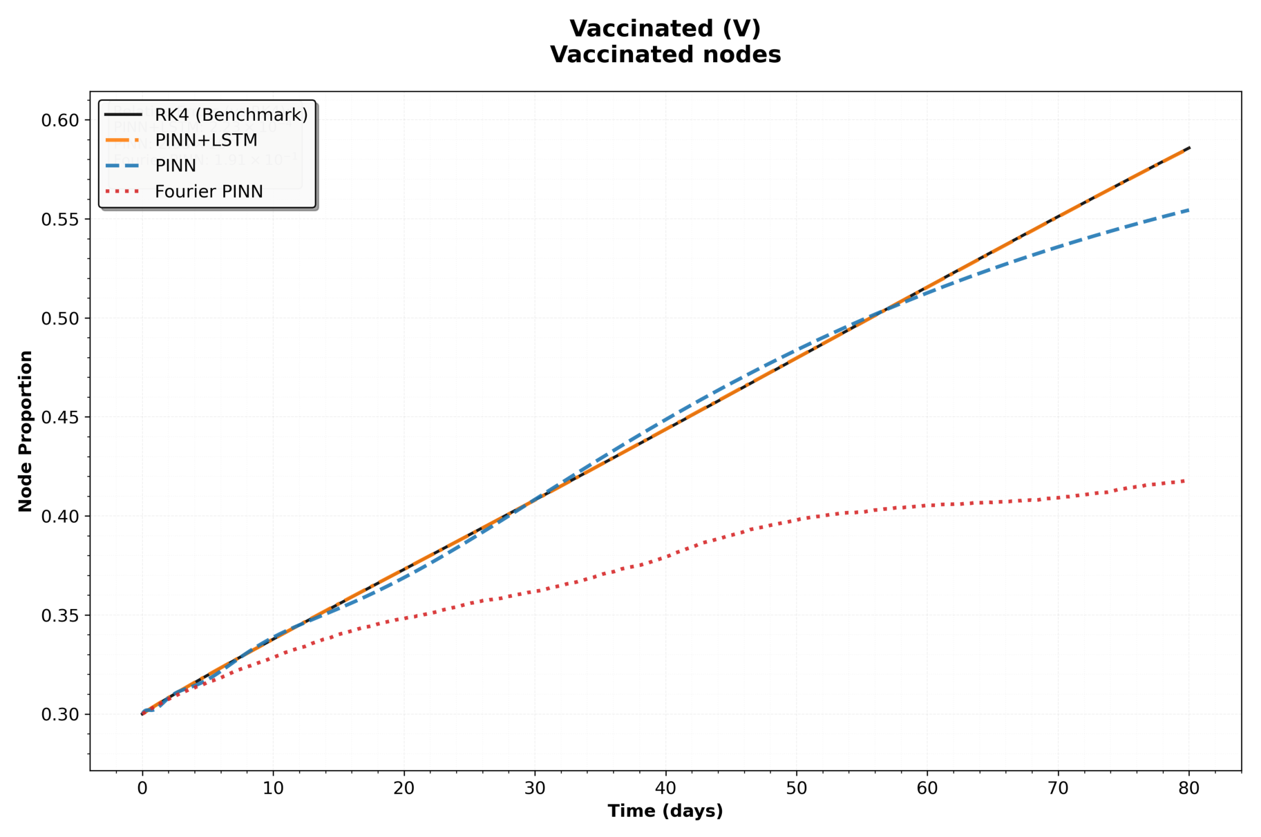
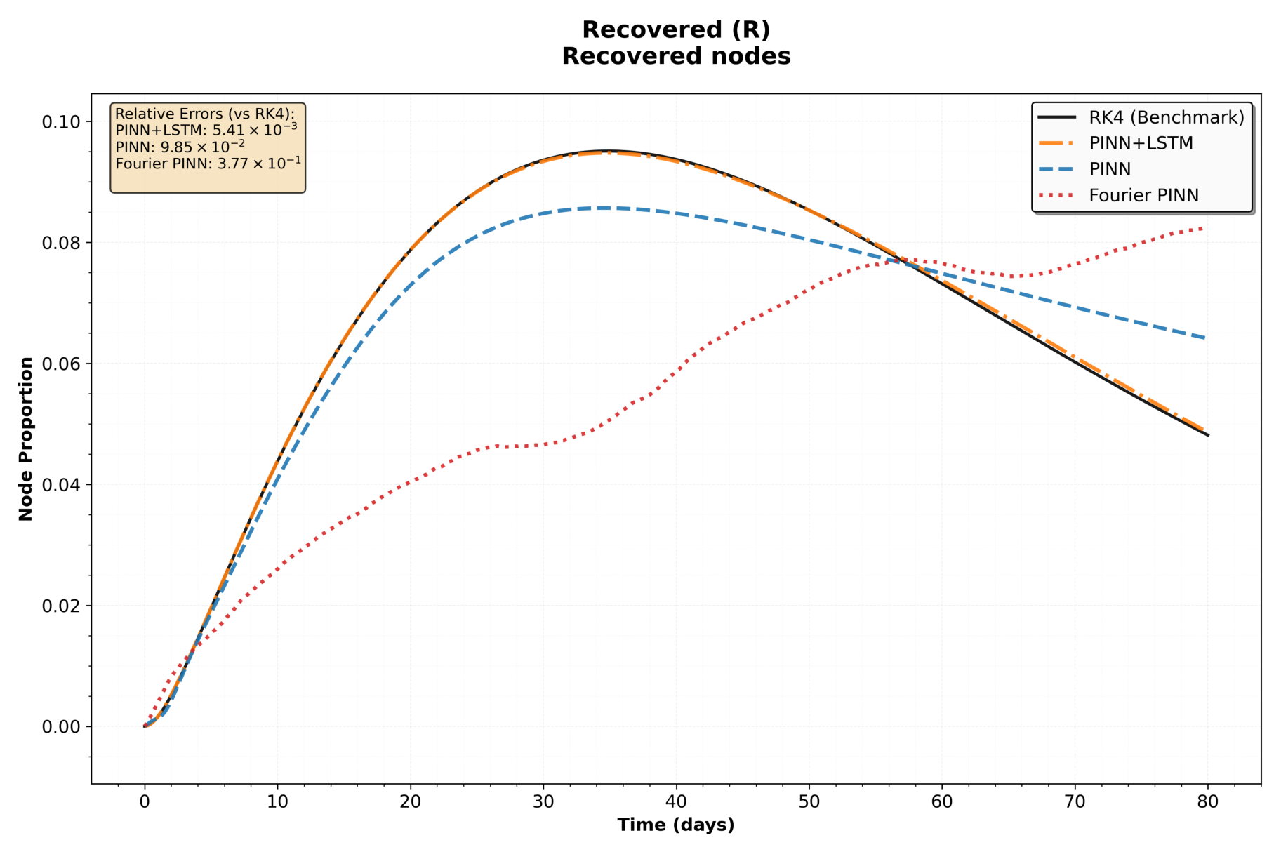
Figure 3, Figure 4, Figure 5, Figure 6, Figure 7, Figure 8 and Figure 9 illustrate the predicted trajectories of all seven state variables. Both models can roughly capture the evolutionary trend. However, PINN + LSTM achieves significantly higher precision, especially for the key compartments E, H, and L, which dominate the epidemic transmission.

Examining each state variable individually, all three methods generally follow the overall evolutionary trend given by the RK4 benchmark. For the Vaccinated (V) compartment, PINN + LSTM achieves exceptional accuracy, while Fourier PINN performs noticeably worse than both PINN and PINN + LSTM. For Susceptible (S) individuals, PINN shows clear deviations in both the declining rate and long-term steady state, while PINN + LSTM maintains tight alignment with the reference solution. In the Exposed (E) compartment, PINN + LSTM closely reproduces the amplitude and timing of the epidemic curve. For High-Risk Infectious (H) and Low-Risk Infectious (L) compartments, PINN + LSTM achieves outstanding consistency with RK4, while both PINN and Fourier PINN display mild to moderate mismatches. In the Quarantined (Q) compartment, Fourier PINN performs significantly worse than PINN and PINN + LSTM, with clear deviations and unstable oscillations, while PINN drifts gradually and PINN + LSTM remains nearly identical to RK4. The Recovered (R) compartment further confirms the superior performance of PINN + LSTM. Overall, although Fourier PINN improves upon the vanilla PINN in some compartments, it performs notably worse in the Vaccinated (V) and Quarantined (Q) states, and PINN + LSTM remains the most accurate and stable method across all variables. This superior performance arises from LSTM’s inherent temporal memory and sequential gating mechanism, which effectively capture time-varying dynamics while complying with physical ODE constraints.

4.3. Error Analysis and Comparison

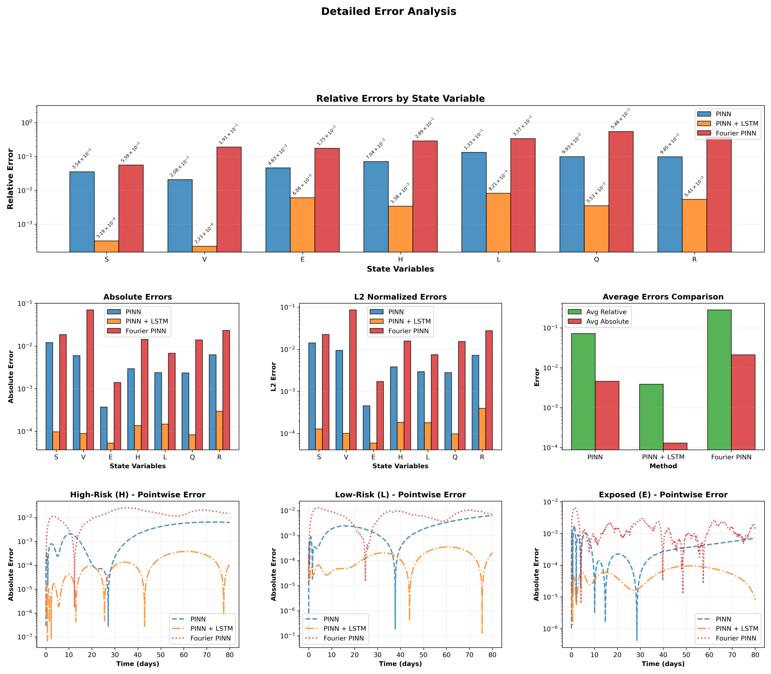
Figure 10 and

Table 1. Quantitative error comparison of PINN + LSTM, PINN, and Fourier PINN across all state variables.

Method	Metric	S	V	E	H	L	Q	R	Avg
PINN + LSTM	Rel	3.19 × 10−4	2.23 × 10−4	6.06 × 10−3	3.38 × 10−3	8.21 × 10−3	3.53 × 10−3	5.41 × 10−3	3.88 × 10−3
	Abs	9.75 × 10−5	8.88 × 10−5	5.31 × 10−5	1.36 × 10−4	1.48 × 10−4	8.32 × 10−5	2.96 × 10−4	1.29 × 10−4
	L2	1.28 × 10−4	1.01 × 10−4	5.93 × 10−5	1.84 × 10−4	1.81 × 10−4	9.88 × 10−5	3.97 × 10−4	1.64 × 10−4
PINN	Rel	3.54 × 10−2	2.08 × 10−2	4.63 × 10−2	7.04 × 10−2	1.33 × 10−1	9.93 × 10−2	9.85 × 10−2	7.20 × 10−2
	Abs	1.20 × 10−2	5.96 × 10−3	3.71 × 10−4	2.94 × 10−3	2.37 × 10−3	2.34 × 10−3	6.19 × 10−3	4.59 × 10−3
	L2	1.42 × 10−2	9.39 × 10−3	4.54 × 10−4	3.83 × 10−3	2.93 × 10−3	2.78 × 10−3	7.23 × 10−3	5.83 × 10−3
Fourier PINN	Rel	5.59 × 10−2	1.91 × 10−1	1.75 × 10−1	2.89 × 10−1	3.37 × 10−1	5.46 × 10−1	3.77 × 10−1	2.81 × 10−1
	Abs	1.84 × 10−2	7.00 × 10−2	1.40 × 10−3	1.43 × 10−2	6.76 × 10−3	1.38 × 10−2	2.31 × 10−2	2.11 × 10−2
	L2	2.24 × 10−2	8.61 × 10−2	1.71 × 10−3	1.57 × 10−2	7.43 × 10−3	1.53 × 10−2	2.77 × 10−2	2.52 × 10−2

present the Relative Error (RE), Absolute Error (AE), and $L_2$ error for each state variable.

Based on the quantitative results, the PINN + LSTM model significantly outperforms both the standard PINN and Fourier PINN across all error metrics. The average relative error is reduced from $7.20\times {10}^{-2}$ for PINN to $3.88\times {10}^{-3}$ for PINN + LSTM, corresponding to a remarkable improvement of 94.61%. Similarly, the average absolute error and average L2 error are reduced by approximately 97.19% compared with the traditional PINN. Meanwhile, Fourier PINN fails to provide competitive accuracy and performs noticeably worse, particularly in the Vaccinated (V) and Quarantined (Q) compartments.

Examining each state variable individually, PINN + LSTM achieves exceptional precision in slowly varying compartments such as S and V, with relative errors of only $3.19\times {10}^{-4}$ and $2.23\times {10}^{-4}$, representing accuracy improvements exceeding 98% over PINN. For infection-dominated states, including H, L, Q, and R, the relative error reductions all exceed 93%, and the relative errors are uniformly controlled within the order of ${10}^{-3}$. Even in the most dynamical Exposed (E) compartment, the relative error is reduced to $6.06\times {10}^{-3}$.

In sharp contrast, the standard PINN shows relatively large deviations, with a relative error as high as $1.33\times {10}^{-1}$ for Low-Risk Infectious (L), and an absolute error for Susceptible (S) nearly 123 times larger than that of PINN + LSTM. Fourier PINN performs even worse, especially in V and Q, with relative errors reaching $1.91\times {10}^{-1}$ and $5.46\times {10}^{-1}$, respectively. These results confirm the clear limitations of purely fully connected PINN and Fourier PINN in capturing sharp transitions and long-term evolutionary dynamics.

Overall, the superior performance of PINN + LSTM validates that introducing temporal memory via the LSTM structure effectively captures the time-dependent characteristics of epidemic transmission and peak dynamics, yielding overwhelming advantages in prediction accuracy, stability, and long-term simulation consistency.

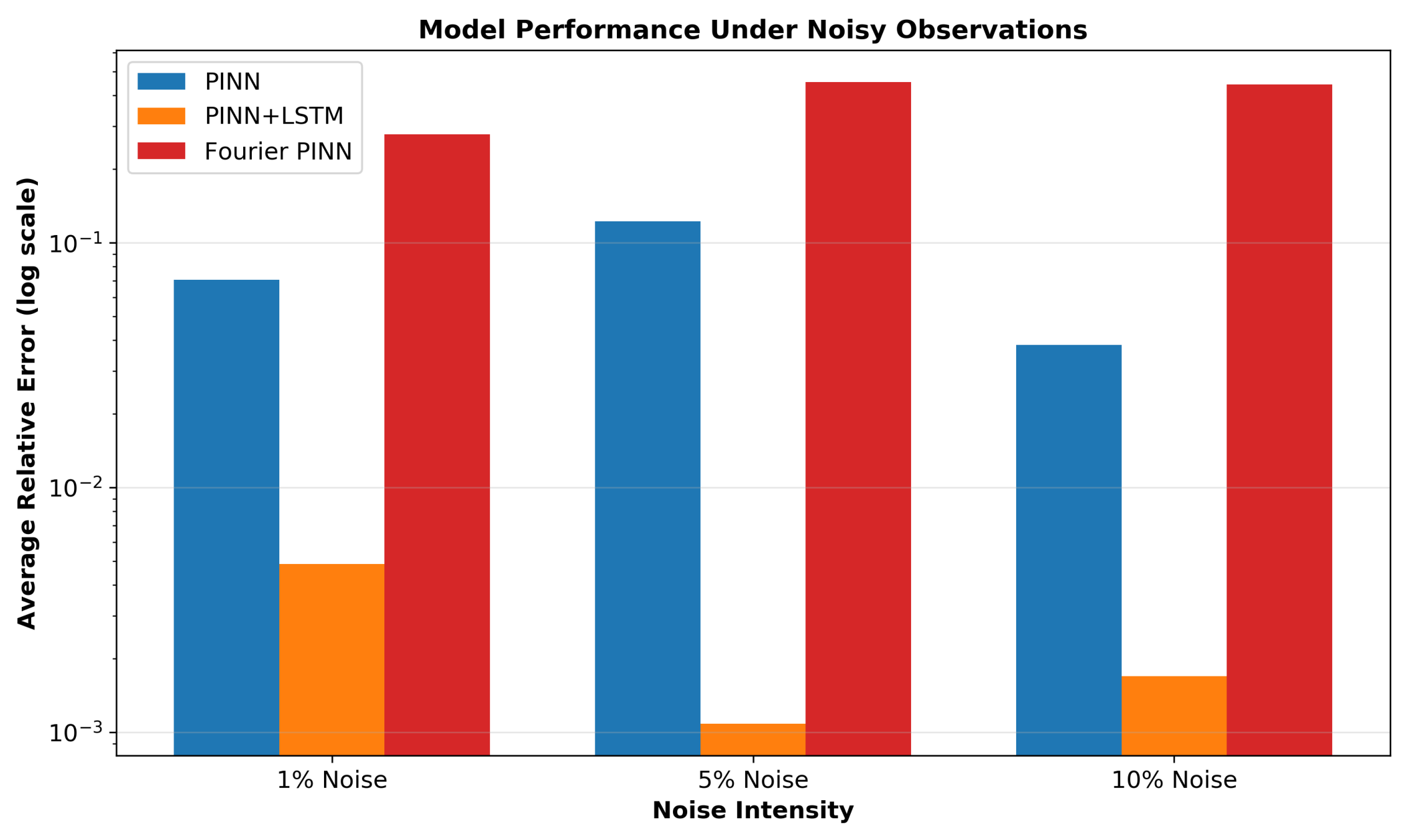
To further validate the robustness of the proposed model in a realistic scenario, we conducted additional experiments by adding Gaussian noise to the observed training data points at three representative levels: 1%, 5%, and 10%. The average relative errors of the PINN + LSTM, standard PINN, and Fourier PINN under different noise intensities are compared, and the results are illustrated in the following figure (Figure 11).

The robustness of the proposed model is validated under three levels of Gaussian noise: 1%, 5%, and 10%. At 1% noise, PINN + LSTM achieves an average relative error of 0.0049, which is far lower than 0.0707 for PINN and 0.2782 for Fourier PINN. When the noise level increases to 5%, the errors of PINN and Fourier PINN rise sharply to 0.1225 and 0.4532, respectively, while PINN + LSTM maintains an extremely low error of 0.0011. Even under strong 10% noise, PINN + LSTM still exhibits superior performance with an error of 0.0017, whereas PINN and Fourier PINN yield much higher errors of 0.0384 and 0.4431. These results confirm that PINN + LSTM possesses stronger noise immunity and more stable dynamic learning ability than both PINN and Fourier PINN in realistic noisy environments.

5. Conclusions

In this paper, we have proposed a novel hybrid framework combining physics-informed neural networks (PINNs) with long short-term memory (LSTM) to model malware propagation dynamics in wireless sensor networks. A seven-compartment SVEHLQR epidemiological model was developed to capture the complex physical interactions among nodes, classifying them into Susceptible (S), Vaccinated (V), Exposed (E), High-Risk Infectious (H), Low-Risk Infectious (L), Quarantined (Q), and Recovered (R) categories. This study’s key contribution lies in integrating LSTM’s temporal memory capability into the PINN architecture, enabling the model to effectively learn time-dependent propagation characteristics.

Using the fourth-order Runge–Kutta (RK4) method as the benchmark, we conducted extensive numerical comparisons among the proposed PINN + LSTM, standard PINN, and Fourier PINN. Experimental results demonstrate that the PINN + LSTM model significantly outperforms both baseline methods across all seven compartments. The average relative error achieved by PINN + LSTM is $3.88\times {10}^{-3}$, compared to $7.20\times {10}^{-2}$ for PINN and $2.81\times {10}^{-1}$ for Fourier PINN, representing a remarkable 94.6% improvement in accuracy over the conventional PINN and an even greater advantage over the Fourier-enhanced version. Particularly noteworthy is its performance on the Vaccinated (V) compartment, where PINN + LSTM attains near-perfect agreement with the RK4 benchmark, with a relative error as low as $2.23\times {10}^{-4}$. Even on the most challenging compartment, Low-Risk Infectious (L), which exhibited a relative error of $1.33\times {10}^{-1}$ for standard PINN and far higher values for Fourier PINN, the proposed method reduces the error to $8.21\times {10}^{-3}$, demonstrating its robustness in capturing complex dynamic behaviors.

It is necessary to clarify why a deep learning solver (PINN + LSTM) is adopted here, even though the 7-dimensional SVEHLQR ODE is low-dimensional, and grid-based methods like RK4 are theoretically feasible. We use RK4 not because it is inadequate for this specific low-dimensional scenario, but as a high-precision benchmark to validate the PINN + LSTM framework. While RK4 performs well in low-dimensional problems, it becomes computationally prohibitive in high-dimensional real-world WSN scenarios (e.g., more compartments, spatial–temporal propagation) due to the curse of dimensionality. Validating PINN + LSTM against RK4 in a low-dimensional setting ensures its reliability, laying the groundwork for its application in complex, high-dimensional scenarios where RK4 is no longer sufficient.

Despite its superior accuracy, the proposed PINN + LSTM framework has certain limitations. The training process is computationally more expensive than standard PINN and Fourier PINN due to the additional LSTM layers, which may hinder its deployment in highly resource-constrained scenarios. Moreover, while the model excels at learning from RK4-generated reference data, its performance on real-world noisy measurements still requires thorough validation. The current study focuses on a fixed parameter configuration, and its generalization ability across different network sizes, topologies, and malware types remains to be fully explored.

Future work will explore several promising directions. First, we plan to validate the model on real-world malware propagation datasets to evaluate its practical reliability. Second, we aim to integrate attention mechanisms or transformer-style structures to further strengthen its long-range temporal dependency modeling. Third, extending the framework to support adaptive and online learning would facilitate real-time threat monitoring and response. Fourth, while the proposed SVEHLQR model represents a meaningful advance for WSN malware modeling by explicitly distinguishing high-risk and low-risk infections, recent research trends from 2025 to 2026 highlight a growing emphasis on spatial–temporal dynamics, especially in the Internet of Underwater Things (IoUT), as well as topology-aware propagation models suitable for the Internet of Vehicles (IoV); thus, we will expand the model to capture these spatial–temporal and topology-aware dynamics to improve its relevance to emerging systems such as IoUT and IoV. Finally, combining the proposed data-driven physics-informed approach with optimal control strategies could lead to a unified framework for both accurate prediction and effective mitigation of malware spread in wireless sensor networks.