Collaborative Scheme for Speed Limit and Illumination at Rural Highway Intersection Based on Drivers’ Ability to Visually Recognize VRUs

Abstract

Poor visibility contributes to nighttime accidents at highway intersections, especially in developing countries where vehicles mix with vulnerable road users (VRUs) such as pedestrians and cyclists. Unlike downtown intersections with traffic signals and ambient lighting, rural intersections have no signals and minimal ambient light, forcing drivers to rely on roadway lighting for hazard recognition. Improving illumination arrangements can significantly reduce the likelihood of crashes. However, there are significant differences in the effects of illumination on drivers’ visual search ability at different vehicle speeds. Therefore, the collaborative matching of illumination and speed limits can effectively improve traffic efficiency and reduce the probability of nighttime accidents. In this paper, we establish a collaborative optimization model of illumination and speed limits at rural highway intersections that considers drivers’ visual recognition of VRUs. We then design an experiment with illuminance, vehicle speed, and VRU type/location as control variables to collect recognition distances, and finally analyze their effects to calculate speed limits under different illuminances. Results indicate that pedestrians and cyclists appearing from the left side are recognized 24.73% and 15.79% earlier than those from the right, suggesting that VRUs from the right side are more vulnerable. Additionally, the safety benefit of improving illumination on increasing speed limits gradually diminishes as illuminance rises. Therefore, determining the most suitable illumination and speed limit configuration requires a comprehensive evaluation of the cost–benefit relationship between lighting investments and the gains resulting from higher speed limits.

1. Introduction

Highway intersections represent highly critical zones for traffic safety due to the simultaneous convergence of multidirectional traffic flows, creating numerous potential conflict points [1,2]. In particular, the conflict is more serious at the highway intersections near villages and towns in some developing countries. The main reasons for this are the mixed traffic of vehicles, pedestrians, non-motor vehicles, and motorcycles, as well as the lack of traffic facilities and imperfect management measures [3]. Meanwhile, poor visibility at unsignalized intersections is widely recognized as a primary catalyst for nighttime collisions [4]. People’s initial intuitive feeling of the nighttime traffic accidents at highway intersections is that the higher the speed, the more accidents. This concept had led many countries to only try to use speed limits to solve traffic safety problems for a long time [5]. However, reducing the speed limit will also reduce transportation efficiency and cause economic losses. Optimizing highway operations therefore dictates that speed limit determinations should be dynamically coupled with other environmental safety variables [6].

In addition to the speed limit, researchers revealed that there is also a close relationship between the illumination of the intersection and traffic safety by analyzing the accident rate. Monsere et al. [7] showed that turning off roadway lighting in Oregon, USA, increased accident rates by 2% to 39%. Similarly, Bullough et al. [8] observed a 12% reduction in collision frequencies at Minnesota intersections equipped with lighting. Data from rural stop-controlled intersections in Iowa further demonstrated that lighting installations decreased nighttime injuries, total accidents, and property damage by 24%, 33%, and 18% [9], respectively. Despite these benefits, the impact of illumination on a driver’s stress response varies heavily with vehicle speed. Therefore, synergizing illumination levels with appropriate speed limits can concurrently boost traffic throughput and lower nighttime accident probabilities.

The existing literature addressing nighttime driving safety through speed limits generally falls into two distinct categories.

The first form of research on speed limits is based on historical accident data and speed distribution law. This method can better describe the operating status of traffic flow and provide guidance for the design of speed limits. For instance, Kokka et al. [10] assessed the impact of a phased implementation of a 20 mph speed limit on road accidents and injuries in Edinburgh, UK, finding that streets with a speed limit of 20 mph had a 10% higher rate of injury reduction compared to streets maintained at 30 mph. Himes et al. [11] evaluated a similar limit increase (65 to 70 mph) on Virginia interstates, noting that roadway improvements could counterbalance the negative safety impacts of higher speeds. Using an artificial neural network (ANN), Ardakani et al. [12] examined head-on rural collisions, incorporating variables like driver demographics and vehicle specifications to determine optimal speed limits for various road types. In the context of expressway maintenance zones, Huang et al. [13] introduced a model for determining nighttime speed limits, based on the empirically observed reduction in speed variance from the advance warning zone to the work zone. Additionally, Sakhare et al. [14] utilized connected vehicle data, finding that motorist compliance with a 55 mph limit improved when digital speed trailers and presence lighting were deployed.

The second research category focuses on driver recognition performance and speed perception. From a micro-perspective, researchers have identified that drivers tend to underestimate their velocity under poor visibility conditions, a critical precursor to accidents [15,16]. Baker et al. [17] demonstrated that in weak lighting, drivers over-rely on flawed speed perceptions, believing they are driving much slower than reality, which prompts speeding. Suh et al. [18] further explained that drivers heavily depend on road illumination and markings for visual stimulation; a lack thereof creates the illusion of sluggish movement, inadvertently encouraging acceleration. This phenomenon was corroborated by Manser and Hancock [19], who observed that bright coatings and wall textures in tunnels heighten visual stimulation, thereby naturally reducing driving speeds and enhancing safety. Pasetto et al. [20] discovered that navigating curves at night impairs speed perception, leading to erratic speed fluctuations and a 45% drop in reaction capabilities. Jgerbrand and Sjbergh [21] utilized adaptive regression models to show that failing to adjust vehicle speed in accordance with visibility is a major driver of nighttime accidents. Furthermore, unreasonable speed limits or poor alignment can degrade visual recognition. Schieber [22] reported that nighttime traffic sign recognition distances shrink by approximately 30% when traveling at 60 mph compared to 5 mph. Building on this, Cheng et al. [23] formulated physical equations linking driving speed with nighttime distance recognition and speed perception. Consequently, they utilized driver characteristics to calculate gradient speed limits upstream of work zones, recommending a maximum nighttime limit of 110 km/h.

In the above two research approaches, the method based on the analysis of historical data can make an overall assessment of speed limit and identify the potentially dangerous road sections effectively. However, this method has two drawbacks. On the one hand, it requires the collection of accident data and vehicle speed data over several years; thus, the potential safety hazards will be ignored for some areas where no traffic accidents have occurred. On the other hand, the incidence of traffic accidents is frequently influenced by multiple factors. Different factors are dynamically interconnected, with varying degrees of influence on accident occurrence, which in turn contributes to the substantial randomness of traffic accidents. Therefore, it is difficult to analyze the impact of each factor on the accident by controlling for variables. The method based on the driver’s visual recognition capabilities does not rely on accident data. It can find the influencing factors of nighttime traffic safety by designing experiments to control for variables and assist relevant departments in selecting a more appropriate speed limit value. Meanwhile, previous studies have also considered many factors, such as illumination, vehicle speed, road alignment, slope, and weather conditions. However, most of the experimental scenarios were carried out when the vehicle or the emergency were stationary. The above two scenarios will overestimate the driver’s nighttime recognition distance, resulting in the parking sight distance required for the design speed limit being greater than the driver’s recognition distance, which creates a safety hazard.

Moreover, substantial variations exist in the shapes and velocities of different VRUs, such as pedestrians and cyclists. The specific locations from which these VRUs emerge also drastically alter a driver’s visual search efficiency, yet this aspect remains largely unexplored in the existing literature [24,25]. For this purpose, we first established a collaborative optimization model of illumination and speed limit at a highway intersection that takes into account the stress response process of drivers to VRUs and their visual recognition characteristics. Secondly, an experiment was conducted by taking lighting conditions, vehicle speed, and the type and location of VRUs as control variables in order to collect data on recognition distances under different scenarios. Based on the collected data, the effects of lighting and vehicle speed on recognition distance were examined for different VRU types and locations. Finally, we calculated and discussed the speed limits under different lighting conditions.

2. Speed Limit and Illumination Collaborative Optimization Model

To enhance both the operational throughput and safety of highway intersections, this study establishes efficiency as the primary objective and safety as the fundamental constraint. When physical intersection lighting cannot be altered, modifying the speed limit is a practical approach to keeping traffic risks within acceptable safety margins. The key symbols and abbreviations used in the model are summarized in

Table 1. The key symbols and abbreviations used in the model.

Symbol	Description	Unit
v	Vehicle speed	km/h
X	Recognition distance	m
S	Safe braking distance	m
L	Residual distance between stopped vehicle and VRU	m
d	Safety buffer distance	m
t1	Brake-free travel time	s
t2	Brake force build-up time	s
ab	Safety braking deceleration	m/s2
E	Illuminance	lx
M	Type of VRU (pedestrian or cyclist)	—
K	Entry position of VRU in driver’s visual field (left or right)	—
ζ	Mean of recognition distance distribution	m
σ	Standard deviation of recognition distance distribution	m
Xs	Safety threshold of recognition distance	m
vm	Optimized speed limit	km/h
abmax	Maximum safety braking deceleration	m/s2

.

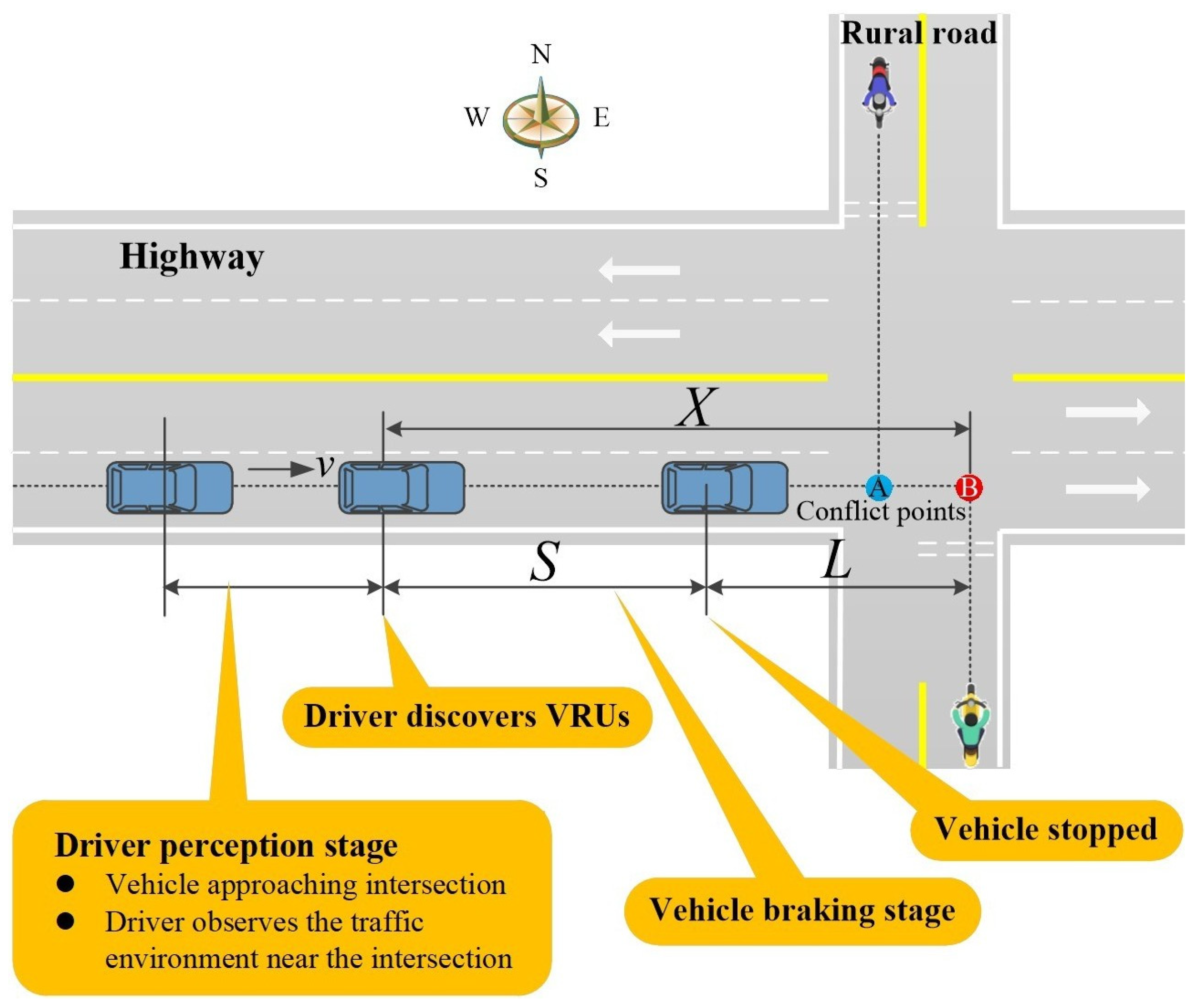
When a driver nears an intersection, their stress response typically follows a specific sequence: monitoring the traffic environment, identifying potential emergencies, and executing evasive maneuvers, such as braking and steering, upon judging a high collision risk until the threat passes. For reference, Figure 1 shows a typical two-way, two-lane, or four-lane highway intersection. Points A and B denote potential collision nodes where vehicles might intersect with VRUs entering from the driver’s left and right visual fields, respectively.

Taking conflict point B as a representative case, let v denote the vehicle’s initial speed prior to the driver spotting the VRU. The parameter X, defined here as the “recognition distance”, represents the spatial gap between the conflict point and the vehicle at the exact moment the driver detects the VRU and applies the brakes. Naturally, a larger X affords the driver more time to take evasive action, thereby lowering the crash probability. Let S represent the safe braking distance, and L represent the residual distance between the stopped vehicle and the VRU. Their relationship is formulated as

$$L=X-S$$

(1)

Based on Equation (1), a successful evasive maneuver requires L to exceed a predefined safety buffer distance d. Thus, the mathematical condition for safe, timely braking is $L>d$.

Drawing on vehicle dynamics, the braking distance S is calculated by

$$S=v\left(t_1+t_2\right)-{\displaystyle \frac{a_b}{6}}{t_2}^2+{\displaystyle \frac{{\left(v-0.5a_b\cdot t_2\right)}^2}{2a_b}}$$

(2)

where t₁ is the brake-free travel time prior to force generation, set as 0.03 s, and t₂ is the time required to build up braking force, set as 0.3 s. The sum of t₁ and t₂ is 0.33 s follows the brake coordination time requirement specified in the Chinese national standard GB 7258-199 [26] which mandates that for vehicles with a gross mass of less than 4.5 tons, the brake coordination time, defined as the interval from the moment the brake pedal is actuated to the moment the braking force reaches 75% of its fully developed value, shall not exceed 0.33 s. In the automotive engineering literature [27], this 0.33 s coordination time is commonly broken down into 0.03 s of brake free-travel time (t₁) and 0.30 s of brake force build-up time (t₂). This classical decomposition remains widely adopted in road safety research and is therefore used in this study. a_b is the safety braking deceleration with a maximum limit of 4.5 m/s² [28], which represents a comfortable deceleration limit for emergency braking scenarios commonly used in road safety research and human factors engineering to avoid passenger discomfort or loss of vehicle control during emergency braking.

Because nighttime lighting generally does not impact a vehicle’s mechanical braking distance, collision avoidance largely depends on the recognition distance X. The driver’s visual performance—and consequently X—is highly sensitive to both intersection illuminance E and vehicle speed v [29]. Furthermore, the type of VRU M and its entry position in the visual field K also critically influence X [30].

Here, we assume that these control variables (E, v, M, K) are independent and that external cognitive factors play a minor role. X follows a normal distribution characterized by a conditional probability density function p(X|E, v, M, K). Let ζ(E, v, M, K) and σ(E, v, M, K) denote the mean and standard deviation of X, respectively. The distribution is given by

$$p\left(X\left|E,v,M,K\right.\right)={\displaystyle \frac{1}{\sqrt{2\pi }\sigma \left(E,v,M,K\right)}}\exp \left(-{\displaystyle \frac{{\left[X-\xi \left(E,v,M,K\right)\right]}^2}{2\sigma {\left(E,v,M,K\right)}^2}}\right)$$

(3)

To guarantee adequate reaction time, the safety threshold X_s is established at the boundary of the 95% confidence interval.

To ensure that drivers can detect VRUs in time, we take the recognition distance at the boundary of the 95% confidence interval as the safety threshold. This ensures that, under specific lighting conditions, the probability of the driver’s recognition distance exceeding the necessary threshold remains at least 95%. This requirement is mathematically expressed as

$$P_X\left(X\le X_s\right)={\displaystyle {\int }_0^{X_s}p\left(X\left|E,v,M,K\right.\right)}dX\ge 0.95$$

(4)

According to the above analysis, the collaborative optimization model of the speed limit and illuminance at a highway intersection is shown as Equation (5), where V_m is the optimized speed limit for nighttime highway intersections.

$$\begin{array}{l}{V}_m=\max v\\ \mathrm{s}.\mathrm{t}. \left\{\begin{array}{l}{\displaystyle {\int }_0^{X_s}p\left(X\left|E,v,M,K\right.\right)}dX\ge 0.95\\ X_s-S>d\\ S=v\left(t_1+t_2\right)-{\displaystyle \frac{a_b}{6}}{t_2}^2+{\displaystyle \frac{{\left(v-0.5a_b\cdot t_2\right)}^2}{2a_b}}\\ a_b\le a_b^{\max }\end{array}\right.\end{array}$$

(5)

According to Equation (5), it is necessary to obtain the driver’s recognition distance for different VRUs under different illumination and vehicle speed scenarios when calculating the optimal speed. In the following text, the collection and analysis of recognition distance will be completed through designing multi-factor experiments.

3. Experimental Design and Data Collection

3.1. Experimental Design

The purpose of the experiment is to collect recognition distances under different scenarios by adjusting the illumination, vehicle speed, and the type and location of VRUs, and to analyze the impact of illumination and vehicle speed on recognition distance under different types and locations of VRUs.

The illumination was divided into four degrees in the experiment. According to the lighting standard, the illuminance at the intersection should not exceed 36 lx, otherwise the excessive illumination will make the headlamps of other vehicles less obvious, which will increase the likelihood of nighttime crashes. Therefore, the four illumination schemes were selected at equal intervals within the normal illumination range. The illuminance corresponding to the four illumination schemes is 0 lx, 12 lx, 24 lx, and 36 lx, respectively.

The vehicle speeds were set to 30 km/h, 40 km/h, 50 km/h, 60 km/h, 70 km/h, and 80 km/h at different illumination schemes. During the trials, participants were required to maintain these specified constant speeds. It should be noted that the speed range of 30–80 km/h in this experiment represented the vehicle’s approach speed before deceleration, not the crossing speed at the intersection conflict point. On rural highways in China, design speeds can reach 80 km/h for Class II highways and 60 km/h for Class III highways according to the Highway Engineering Technical Standard (JTG B01-2014) [31]. Before decelerating for an intersection, drivers might initially travel at these speeds. Therefore, testing the full range from free-flow speed (50–80 km/h) to decelerated speed (30–50 km/h) allowed us to (1) capture the upper bound of approach speeds that drivers might encounter under real-world conditions, especially on higher-class rural highways; (2) establish a continuous relationship between approach speed, illuminance, and VRU recognition distance, which was essential for the collaborative optimization model proposed in this study; and (3) address nighttime conditions where low traffic volume might lead to higher approach speeds. Lower speeds within the tested range (30–50 km/h) represented conditions when drivers have already decelerated in response to the intersection or traffic conditions.

VRUs were programmed to emerge from either the left or the right visual periphery of the intersection. Upon reaching a predetermined spatial threshold relative to the collision node, termed the “trigger distance”, the system automatically generated a VRU. Participants were instructed to execute an emergency stop the exact moment they visually detected the VRU.

3.2. Experimental Scenario Construction

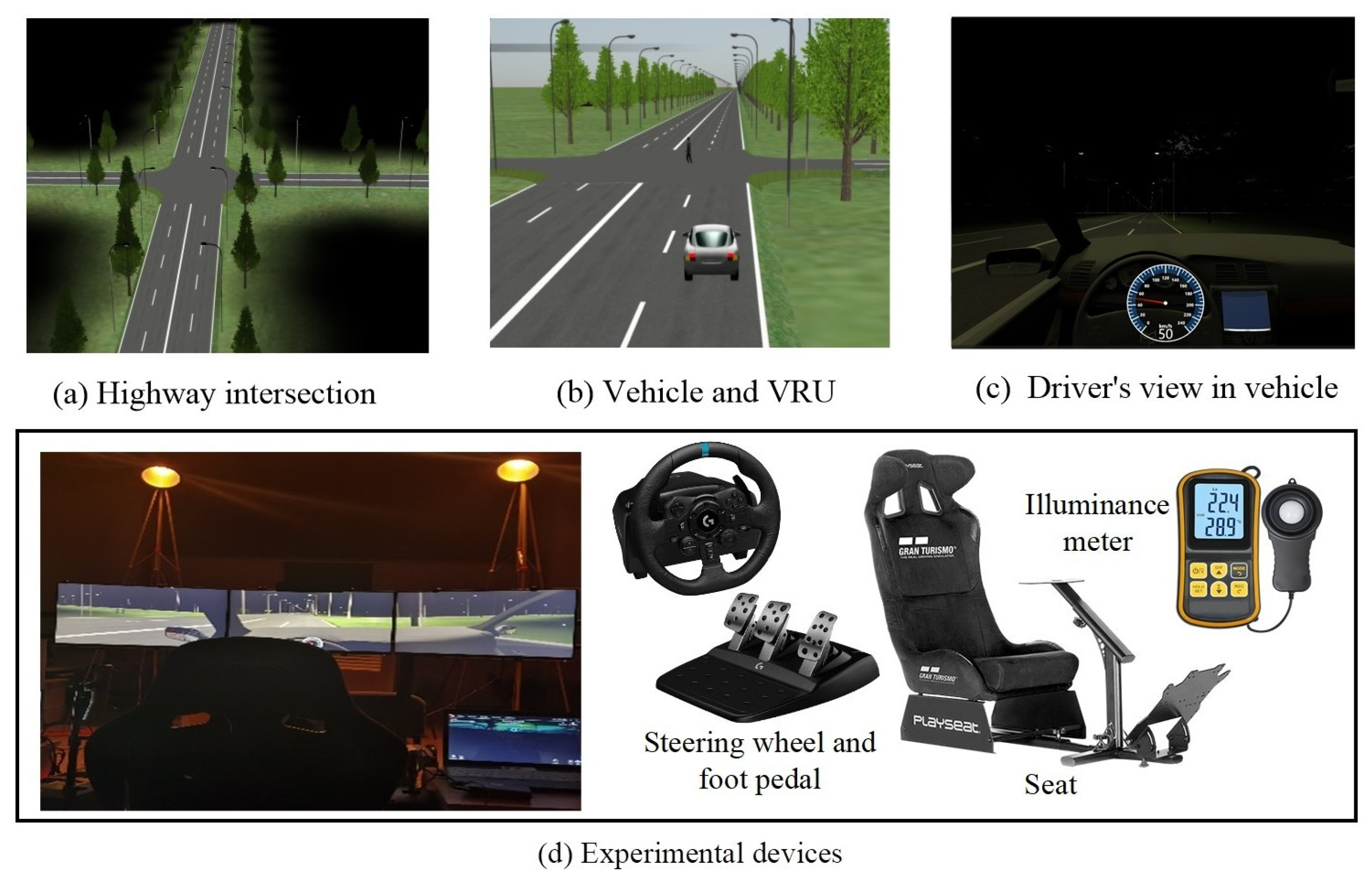
Given the profound safety hazards and uncontrollable variables inherent in real-world driving studies on open roads, the experiments were safely conducted using an advanced indoor simulation framework. This highly regulated environment was constructed by integrating a driving simulator with a precisely controlled lighting apparatus, ensuring consistent and repeatable research scenarios. The driving simulator used in this study consisted of an integrated dashboard, steering wheel, accelerator, and brake pedals, and three forward-facing displays providing a 130° horizontal field of view. The simulation scenarios were developed using UC-win/Road 13 software, which allows for precise control of road geometry, intersection design, vehicle dynamics, and VRU behavior. The UC-win/Road simulator was selected for the following reasons: (1) the simulator allows seamless integration with external lighting apparatus, enabling accurate and repeatable control of illuminance levels at the driver’s eye position; (2) the software enables precise programming of VRU emergence timing, location, and type, which is essential for our experimental design; (3) the simulator allows us to conduct emergency braking scenarios without any risk to participants or equipment.

Figure 2 shows the visual setup of these simulated environments. Figure 2a presents an overview of the simulated rural highway intersection used in the experiment. The intersection is a typical two-way, two-lane or four-lane unsignalized rural highway intersection. The vehicle approaches the intersection from the bottom of the image, and the surrounding environment is characterized by the absence of traffic signals and ambient lighting, consistent with real-world rural intersection conditions. Figure 2b illustrates the spatial relationship between the vehicle and a vulnerable road user (VRU) near the intersection. Figure 2c shows the driver’s in-vehicle perspective during the experiment. Figure 2d shows the actual experimental devices, including the driving simulator cabin, the lighting apparatus, and the display screens.

VRUs in the experiment were divided into two models: pedestrian and cyclist. Because the speeds of the two VRUs are different, we selected TTC as the judgment indicator to calculate the initial distances from the two VRUs to the conflict point and the trigger distances at different speeds. Assuming a VRU velocity of v_E and a TTC denoted as t_E, the initial distances of VRUs to the conflict point S_E can be expressed by Equation (6) as follows:

$$S_E=v_E{t}_E$$

(6)

To guarantee that drivers had ample visual scanning duration before a potential conflict, t_E was standardized at 20 s.

According to the definition of TTC, when the vehicle speed is v, the trigger distance can be expressed by Equation (7) to ensure that the vehicle can conflict with VRUs.

$$S_T={\displaystyle \frac{S_E}{v_E}}v$$

(7)

The values of S_E under two VRUs and trigger distances at different vehicle speeds were calculated according to Equations (6) and (7), as shown in

Table 2. The values of S_E for two VRUs.

VRU	vE (km/h)	SE (m)
Pedestrian	4	22
Cyclist	12	67

and

Table 3. The values of trigger distances at different vehicle speeds.

Vehicle Speed (km/h)	ST (m)
80	444
70	389
60	333
50	278
40	222
30	167

, respectively.

3.3. Participants

The participant pool consisted of 100 licensed drivers, comprising 67 males and 33 females. This specific gender distribution was intentionally selected to mirror the current 7:3 male-to-female driver demographic ratio in China. The participants’ ages ranged from 22 to 35 years, reflecting a mean age of 26.17 and a standard deviation of 2.72.

Inclusion criteria: (a) holding a valid driver’s license for at least two years; (b) normal or corrected-to-normal vision; (c) no self-reported history of night blindness, color blindness, or other visual disorders; and (d) no self-reported history of neurological or cardiovascular conditions that could affect driving performance.

Exclusion criteria: (a) inability to complete the practice session without simulator sickness; (b) failure to follow experimental instructions during the practice session; and (c) self-reported fatigue or sleep deprivation on the day of the experiment.

Informed consent: All participants were informed of the experimental procedures, including the duration of the experiment, the use of a driving simulator, and the emergency stop task. Participants were assured that they could withdraw from the experiment at any time without penalty. Written informed consent was obtained from all participants prior to the experiment.

3.4. Data Collection

Measured variables: The experiment involved four independent variables: illuminance E (four levels: 0, 12, 24, 36 lx), vehicle speed v (six levels: 30, 40, 50, 60, 70, 80 km/h), VRU type M (two levels: pedestrian, cyclist), and VRU entry position K (two levels: left, right). The dependent variable was the recognition distance X, defined as the distance between the vehicle and the conflict point at the moment the driver first detected the VRU and initiated braking.

Instruments and devices: The experiment was conducted using a UC-win/road driving simulator. The lighting conditions were controlled using a programmable LED lighting system capable of producing illuminance levels of 0, 12, 24, and 36 lx at the driver’s eye position, measured with a digital luxmeter. Vehicle speed, brake pedal activation timing, and brake pedal force were automatically recorded by the simulator’s data acquisition system.

Trial design: Two types of VRUs (pedestrian and cyclist) appeared randomly from two directions (left and right) of the driver’s visual field under four illumination levels and six vehicle speeds, resulting in 96 experimental trials (2 × 2 × 4 × 6 = 96). In addition, 48 catch trials (no VRU appearance) were randomly interspersed under the same four illumination levels and six speed levels. Catch trials prevented anticipatory responses and maintained ecological validity, since VRUs do not appear at every intersection in real-world driving. Thus, each driver completed a total of 144 tests (96 experimental trials + 48 catch trials).

Practice session: Before the formal experiment, each driver completed a 20 min practice session to become familiar with the vehicle’s braking performance, driving environment, and speed control ability.

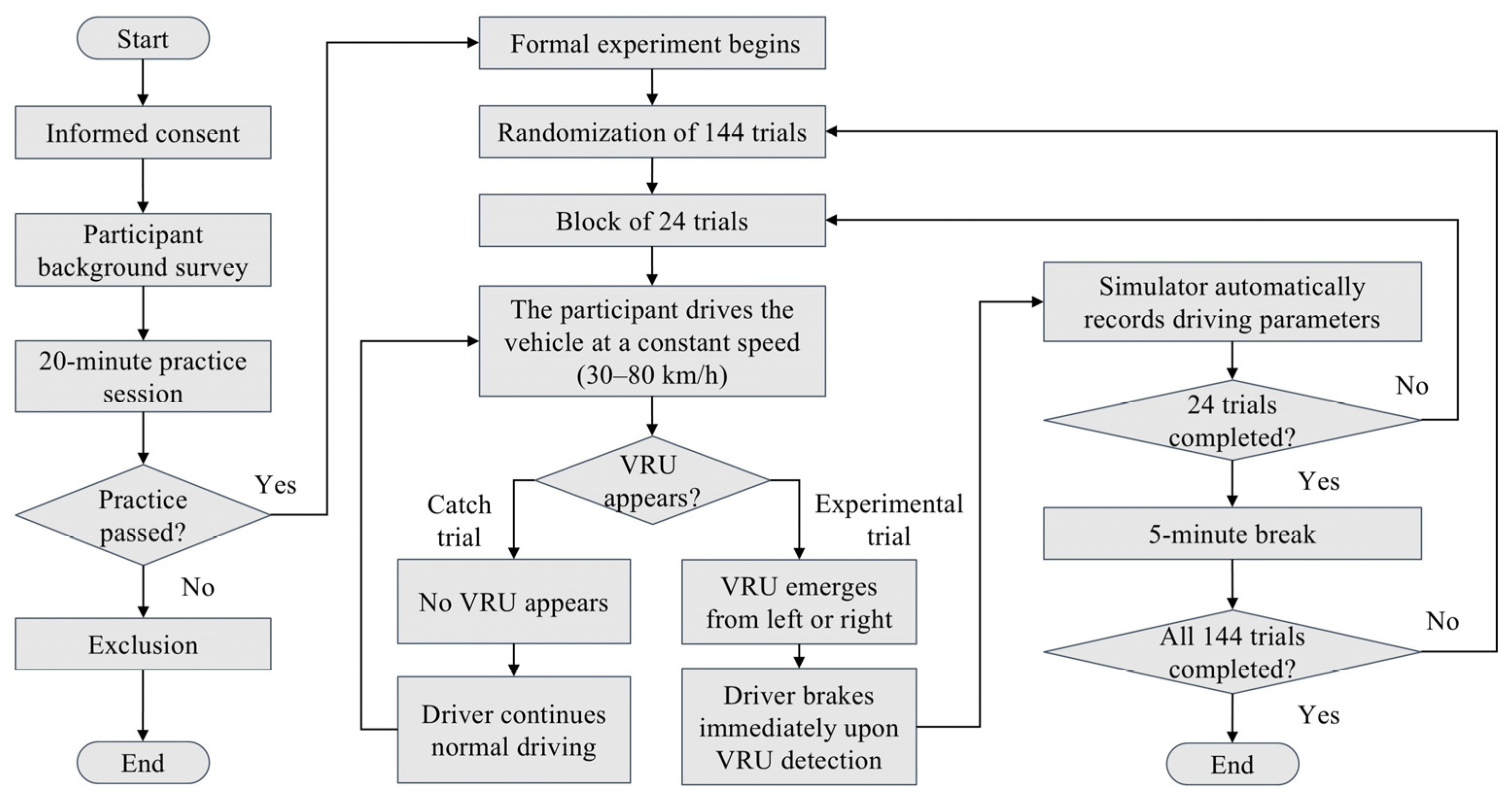
Experimental procedure: The presentation order of the 144 trials was randomized for each participant to minimize order effects. Figure 3 presents a flowchart of the experimental procedure. The overall experimental procedure was as follows:

Step 1: The driver drove the vehicle at a constant speed corresponding to the current speed limit (30, 40, 50, 60, 70, or 80 km/h). During this process, a VRU was automatically triggered at a specific location (or no VRU appeared for catch trials). If the driver detected a VRU, they were instructed to brake immediately until the vehicle came to a complete stop.

Step 2: The simulator’s data acquisition system automatically recorded the driver’s driving parameters, including recognition distance (m) and brake pedal activation time (ms).

Step 3: After completing 24 trials, the driver took a 5 min rest before starting the next trial. Steps 1 and 2 were repeated until all 144 trials were completed.

4. Results

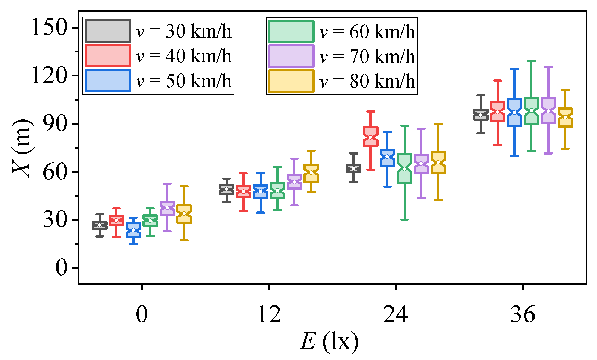
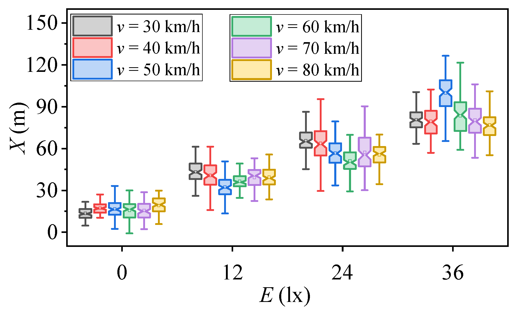
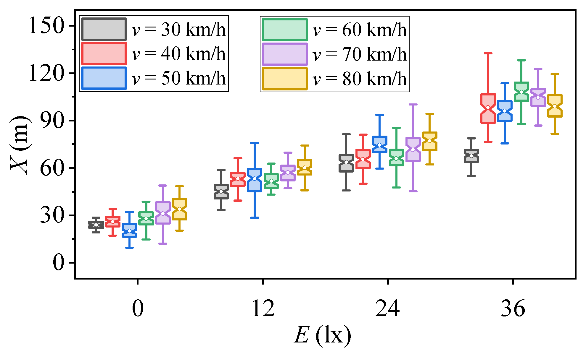
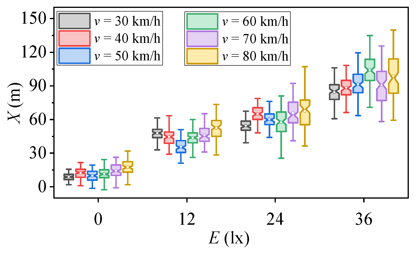
The recognition distance data for pedestrians and cyclists under different illuminances and speeds are extracted, as shown in Figure 4, Figure 5, Figure 6 and Figure 7, respectively. Figure 4 and Figure 5 are the recognition distances for pedestrians on the left and right sides of the driver’s visual field, respectively. Figure 6 and Figure 7 are the recognition distances for cyclists on the left and right sides of the driver’s visual field, respectively.

From Figure 4, Figure 5, Figure 6 and Figure 7, it can be seen that with the increase in illumination, drivers’ visual recognition distances for pedestrians and cyclists exhibit an upward trend, while the gap between the two distances gradually widens.

Right-Side Emergence Analysis: The average recognition distances for the pedestrians for the four lighting conditions investigated are 16.29 m, 38.59 m, 58.34 m, and 83.46 m, corresponding to illuminance levels of 0 lx, 12 lx, 24 lx, and 36 lx, respectively. As the illuminance increased from 0 lx to 36 lx, the recognition distance for pedestrians increased by 67.17 m. Additionally, at vehicle speeds of 30 km/h, 40 km/h, 50 km/h, 60 km/h, 70 km/h, and 80 km/h, the average recognition distances for pedestrians are 50.74 m, 50.31 m, 51.4 m, 46.69 m, 48.13 m, and 47.73 m, respectively. In this scenario, the average recognition distance under the four illuminances is 49.17 m.

The average recognition distances for the cyclist for the four lighting conditions investigated are 12.43 m, 45.03 m, 61.78 m, and 92.99 m, corresponding to illuminance levels of 0 lx, 12 lx, 24 lx, and 36 lx, respectively. As the illuminance increased from 0 lx to 36 lx, the recognition distance for pedestrians increased by 80.56 m. Additionally, at vehicle speeds of 30 km/h, 40 km/h, 50 km/h, 60 km/h, 70 km/h, and 80 km/h, the average recognition distances for pedestrians are 48.9 m, 52.57 m, 49.31 m, 54.27 m, 54.22 m, and 59.07 m, respectively. In this scenario, the average recognition distance under the four illuminances is 53.06 m.

Left-Side Emergence Analysis: For the pedestrian appearing from the left side of the intersection in the driver’s visual field, the average recognition distances for the pedestrian for the four lighting conditions investigated are 30.08 m, 50.96 m, 67.63 m, and 96.64 m, corresponding to illuminance levels of 0 lx, 12 lx, 24 lx, and 36 lx, respectively. As the illuminance increased from 0 lx to 36 lx, the recognition distance for pedestrians increased by 66.56 m. Additionally, at vehicle speeds of 30 km/h, 40 km/h, 50 km/h, 60 km/h, 70 km/h, and 80 km/h, the average recognition distances for pedestrians are 58.26 m, 64.01 m, 59.43 m, 59.41 m, 63.56 m, and 63.27 m, respectively. In this scenario, the average recognition distance under the four illuminances is 61.33 m.

For the cyclist appearing from the left side of the intersection in the driver’s visual field, the average recognition distances for the pedestrian for the four lighting conditions investigated are 27.12 m, 53.37 m, 69.67 m, and 95.61 m, corresponding to illuminance levels of 0 lx, 12 lx, 24 lx, and 36 lx, respectively. As the illuminance increased from 0 lx to 36 lx, the recognition distance for pedestrians increased by 66.56 m. Additionally, at vehicle speeds of 30 km/h, 40 km/h, 50 km/h, 60 km/h, 70 km/h, and 80 km/h, the average recognition distances for pedestrians are 50.03 m, 60.69 m, 60.96 m, 63.37 m, 66.06 m, and 67.55 m, respectively. In this scenario, the average recognition distance under the four illuminances is 61.44 m.

By comparing the above data, it can be seen that drivers have shorter recognition distances for pedestrians and bicycles appearing from the right side of the intersection compared to those appearing from the left side. Specifically, the recognition distance for pedestrians appearing from the left side of drivers’ visual field is increased by 24.73% compared to those appearing on the right side, and the recognition distance for cyclists appearing from the left side of drivers’ visual field is increased by 15.79% compared to those appearing on the right side. This indicates that drivers find it more challenging to recognize VRUs coming from the right side of their visual field, suggesting that VRUs appearing from the right side are more at risk. This can be attributed to two main factors. Firstly, under the traffic rules of right-hand driving, drivers have a larger visual search space for the left side of the intersection compared to the right side. Secondly, based on post-experiment inquiries about the visual search behavior of the drivers, it was found that due to the potential conflict with VRUs appearing from the left side, most drivers chose to observe the left side of the intersection first before observing the right side. Combining these two factors, it ultimately leads to a higher likelihood of traffic accidents involving conflicts between vehicles and VRUs appearing from the right side of the intersection under the same lighting conditions and vehicle speeds. Therefore, when designing nighttime speed limits for highway intersections, it is crucial to consider the impact of pedestrians and cyclists appearing from the right side of the intersection in drivers’ visual field on traffic safety.

5. Discussion

5.1. Factors Influencing Recognition Distance

To explore the impact of illuminance and vehicle speed on recognition distance, we analyze the 4800 recognition distance data collected in the scenarios of pedestrians and cyclists appearing from the right side of drivers’ visual field. The Spearman correlation coefficients between the recognition distance for pedestrians and cyclists and the illuminance are 0.934 (p < 0.01) and 0.933 (p < 0.01), respectively, which indicates that the recognition distance is significantly affected by the illuminance at night. The Spearman correlation coefficients between the recognition distance for pedestrians and cyclists and the vehicle speed are 0.087 and −0.044, which shows that the correlation between recognition distance and vehicle speed is not significant when the vehicle speed is in the range of [30 km/h, 80 km/h]. Therefore, when establishing the recognition distance model of pedestrian and cyclist emergencies, we only take the illuminance as the influencing factor.

We use the KS-test to test the normality of the recognition distance at different illuminance levels. The KS-test results of recognition distance at four illuminations are shown in

Table 4. KS-test results of recognition distance at four illuminance levels.

VRU	E (lx)	ξ (m)	σ (m)
Pedestrian	0	16.289	3.759
	12	38.579	5.834
	22	58.340	9.386
	36	83.463	10.638
Cyclist	0	12.430	3.383
	12	45.028	5.957
	22	61.781	9.617
	36	92.994	13.308

, where ξ and σ are the mean and the standard deviation of recognition distance, respectively. The results show that the recognition distances at the four illuminations all obey the normal distribution.

The mean recognition distances for pedestrians and cyclists are represented by ${\xi }_{\mathrm{p}}$ and ${\xi }_{\mathrm{b}}$, respectively, and the standard deviations of recognition distances for pedestrians and cyclists are represented by ${\sigma }_{\mathrm{p}}$ and ${\sigma }_{\mathrm{b}}$, respectively. Linear regression is used to fit the relationship between ${\xi }_{\mathrm{p}}$, ${\xi }_{\mathrm{b}}$, and E. The relationships between ${\xi }_{\mathrm{p}}$, ${\xi }_{\mathrm{b}}$, and E can be expressed as Equations (8) and (9). The R² of the two equations is larger than 0.95 for all cases, indicating that the linear regression model given in Equations (8) and (9) effectively fits the mean of recognition distance for pedestrians and cyclists.

$${\xi }_{\mathrm{p}}=15.975+1.844E$$

(8)

$${\xi }_{\mathrm{b}}=14.292+2.154E$$

(9)

The quadratic polynomial regression is used to fit the relationship between E and ${\sigma }_{\mathrm{p}}$, ${\sigma }_{\mathrm{b}}$. The relationships between ${\sigma }_{\mathrm{p}}$, ${\sigma }_{\mathrm{b}}$, and E can be expressed as Equations (10) and (11). The R² of the two equations is larger than 0.95 for all cases, indicating that the quadratic polynomial regression model given in Equations (10) and (11) effectively fits the standard deviation of recognition distance for pedestrians and cyclists.

$${\sigma }_{\mathrm{p}}=-0.001E^2+0.253E+3.57$$

(10)

$${\sigma }_{\mathrm{b}}=0.002E^2+0.209E+3.33$$

(11)

The recognition distances for pedestrians and cyclists are represented by $X_{\mathrm{p}}$ and $X_{\mathrm{b}}$, respectively. According to Equations (8)–(11), the distribution functions of $X_{\mathrm{p}}$ and $X_{\mathrm{b}}$ can be expressed as Equations (12) and (13), respectively.

$$X_{\mathrm{p}} ~ N\left({\xi }_{\mathrm{p}},{\sigma }_{\mathrm{p}}\right)=N\left(\left(15.975+1.844E\right),{\left(-0.001E^2+0.253E+3.57\right)}^2\right)$$

(12)

$$X_{\mathrm{b}} ~ N\left({\xi }_{\mathrm{b}},{{\sigma }_{\mathrm{b}}}^2\right)=N\left(\left(14.292+2.154E\right),{\left(0.002E^2+0.209E+3.33\right)}^2\right)$$

(13)

To improve the safety of the highway intersection, we select the recognition distance under one sigma level as the design standard of nighttime speed limit at the highway intersection. According to Equations (12) and (13), $X_{\mathrm{p}}$ and $X_{\mathrm{b}}$ under 1 sigma level can be expressed as Equation (14) and Equation (15), respectively.

$$X_{\mathrm{p}}={\xi }_{\mathrm{p}}-1.645{\sigma }_{\mathrm{p}}=0.0016E^2+1.428E+10.102$$

(14)

$$X_{\mathrm{b}}={\xi }_{\mathrm{b}}-1.645{\sigma }_{\mathrm{b}}=-0.0033E^2+1.81E+8.814$$

(15)

The maximum speeds of cyclists and pedestrians are represented by $v_{\mathrm{p}}$ and $v_{\mathrm{b}}$, respectively. By substituting Equations (14) and (15) into Equation (5), $v_{\mathrm{p}}$ and $v_{\mathrm{b}}$ can be expressed as Equation (16) and Equation (17), respectively.

$$v_{\mathrm{p}}=\sqrt{25.92\left(0.0016E^2+1.428E+10.102-d\right)}$$

(16)

$$v_{\mathrm{b}}=\sqrt{25.92\left(-0.0033E^2+1.81E+8.814-d\right)}$$

(17)

Due to cyclists and pedestrians appearing randomly at highway intersections, we take the minimum value of the maximum speed of cyclists and pedestrians as the nighttime speed limit. We calculate the minimum illuminance E_min under different speed limits at highway intersections and the additional illuminance △E required for each 10 km/h speed limit increase; the calculated results are shown in Table 4. It can be seen that △E increases with the increase in speed limit, which indicates that the benefit of improving illumination on increasing speed limit gradually becomes lower. Therefore, on the premise of ensuring traffic safety, in order to improve traffic efficiency and save economic cost, it is necessary to determine the most appropriate lighting and speed limit scheme in combination with the ratio of illumination cost to the benefits from increasing speed limits.

Because intersection VRU encounters are highly unpredictable, the ultimate nighttime speed limit must be dictated by the more conservative (minimum) value between $v_{\mathrm{p}}$ and $v_{\mathrm{b}}$. Calculations determining the minimum required illuminance E_min for incremental speed limits, alongside the marginal illuminance △E needed for each successive 10 km/h increment, are presented in

Table 5. Minimum illuminance E_min under different speed limits at highway intersection and the additional illuminance △E required for each 10 km/h speed limit increase.

Vm (km/h)	Emin (lx)	△E (lx)
20	0	—
30	1.18	1.18
40	5.23	4.05
50	11.42	6.19
60	18.97	7.55
70	27.80	8.83
80	37.86	10.06

. Crucially, as the target speed limit scales upwards, the △E requirement expands disproportionately, indicating a diminishing marginal return on safety benefits derived purely from adding more light. Consequently, traffic engineers must meticulously balance the economic expenditures of high-intensity illumination against the operational gains of elevated speed limits to finalize an optimal intersection management scheme.

5.2. Comparison with the Existing Literature

A central finding of this study is that drivers recognize VRUs emerging from the left side earlier than those from the right side (24.73% for pedestrians and 15.79% for cyclists), indicating that VRUs appearing from the right visual field pose a greater safety risk at rural unsignalized intersections. To understand the generalizability and boundary conditions of this finding, we compare it with existing studies that have reported contradictory, supportive, or variable results regarding directional asymmetry in driver visual attention and response.

(1)

Contradictory studies

Several studies have reported that drivers react faster to stimuli emerging from the right side. Jurecki and Stańczyk [32,33,34] conducted a series of driving simulator experiments and found that driver reaction times to lateral entering pedestrians were shorter when the pedestrian appeared from the right compared to the left. Stanisław Jurecki et al. [35] further confirmed this pattern in complex road incidents. At first glance, these findings appear to contradict our results. However, several methodological differences may explain the discrepancy.

Firstly, the reaction time tasks in those studies were relatively simple, requiring drivers to respond as quickly as possible to a single, expected stimulus. In contrast, our experiment required drivers to continuously monitor both sides of the intersection without knowing when or where a VRU would appear, which more closely resembles real-world visual search. Secondly, the driving scenarios differed substantially. Jurecki and Stańczyk’s experiments were conducted on a straight road section with a pedestrian entering from the roadside, whereas our study specifically focused on intersection scenarios where drivers must simultaneously attend to multiple potential threat directions. Thirdly, the dependent variable differs: our study measured recognition distance (i.e., how far in advance a driver detects a VRU), while reaction time studies measure the time from stimulus onset to brake application. These two measures are related but not equivalent, as recognition distance is influenced by both reaction time and vehicle speed.

Therefore, while drivers may react faster to right-side stimuli in simple, single-task conditions, the spatial asymmetry may reverse or diminish in more complex intersection scenarios requiring sustained visual search.

(2)

Supporting studies

Our findings align with those of several studies reporting left-side attentional bias or a neglect of the right side in driving contexts. Kaya et al. [36] conducted an on-road study and found that drivers frequently failed to scan to the right when turning, leading to near-misses with pedestrians and cyclists. Ahlström et al. [37] reported that at urban intersections, drivers’ visual attention was disproportionately directed to the left when crossing paths with cyclists, resulting in reduced attention to the right side. Werneke and Vollrath [38] found that intersection characteristics significantly influenced driver attention allocation, with the right side often receiving less visual attention than the left.

These findings, together with our results, suggest a consistent pattern: under conditions of high cognitive load or complex visual environments, drivers tend to prioritize the left visual field. This left-side bias may be explained by hemispheric asymmetries in visual attention, where the right hemisphere (which processes the left visual field) is specialized for sustained attention and vigilance. Alternatively, it may reflect learned scanning patterns: in right-hand traffic countries (such as China), drivers may develop a habitual priority for checking the left side first due to the expectation of oncoming traffic and potential conflicts from that direction.

(3)

Studies showing variability

Several studies have reported that directional asymmetry varies significantly depending on contextual factors. Li et al. [39], using naturalistic driving data in China, found that driver visual scanning behavior at intersections was influenced by signalization, traffic volume, and time of day, with no fixed directional bias. Kircher and Ahlström [40] reported that attentional requirements for drivers and cyclists at intersections varied dynamically depending on vehicle speed, proximity to the intersection, and the presence of other road users. Boda et al. [41] compared test track and driving simulator responses to a cyclist crossing the path and found that response patterns varied significantly between the two environments, suggesting that experimental setup may moderate observed effects.

These studies highlight that directional asymmetry is not a fixed phenomenon but rather depends on multiple factors, including intersection type (signalized vs. unsignalized), traffic volume, time of day, and experimental paradigm. Our finding of right-side danger should therefore be interpreted within specific boundary conditions.

(4)

Boundary conditions and applicability of our finding

Based on the above comparison, our finding that VRUs from the right side are more dangerous is applicable under specific boundary conditions. This finding applies to rural unsignalized intersections during nighttime conditions with low ambient lighting, where drivers must rely almost exclusively on roadway lighting for hazard recognition. This finding is specifically relevant to pedestrians and cyclists as vulnerable road user types, and it assumes a continuous visual search task in which drivers do not know when or where a VRU will appear, rather than a simple reaction time task. The finding also assumes low traffic volume conditions where no other vehicles are present to guide the driver’s visual attention, and it is based on recognition distance as the dependent variable rather than reaction time. Additionally, the finding is derived from right-hand traffic countries (such as China, the United States, and continental Europe), where drivers have a larger visual search space for the left side of the intersection due to oncoming traffic.

Under different conditions, such as signalized intersections, daytime lighting, simple reaction time tasks, high traffic volume, or left-hand traffic countries, the directional asymmetry may differ or even reverse. Future research should systematically investigate these moderating factors to further refine the applicability of our findings.

6. Conclusions

This research focused specifically on rural highway intersections, which differ from downtown intersections in two critical aspects: absence of traffic signals and negligible ambient lighting from surrounding buildings. These characteristics mean that rural intersections rely almost exclusively on roadway lighting for hazard recognition, and drivers must depend on their own visual search to detect vulnerable road users. We formulated a joint optimization framework integrating speed limits and lighting to elevate nighttime safety at rural highway intersections, specifically factoring in drivers’ visual perception and stress reactions to VRUs. The aim of this optimization was to obtain the maximum speed of vehicles safely passing through the intersection according to illumination. To empirically ground this model, an indoor simulation was conducted where pedestrians and cyclists emerged from both the left and right peripheral fields of the drivers, providing the foundational data for our calculations. The principal findings of this study are summarized below.

Analysis revealed a pronounced spatial asymmetry in hazard recognition: drivers identified pedestrians and cyclists originating from the left side 24.73% and 15.79% earlier, respectively, than those approaching from the right. This indicates that drivers find it more challenging to recognize VRUs coming from the right side of their visual field. In rural intersections without signal control, this asymmetry is particularly critical because drivers rely entirely on visual search without the aid of traffic signals.

While enhanced illumination consistently expanded the drivers’ visual detection range, vehicle speed (within the tested 30 to 80 km/h spectrum) exhibited negligible correlation with recognition distance, yielding statistically insignificant Spearman coefficients of 0.087 for pedestrians and −0.044 for cyclists. The relationship between recognition distance and illuminance can be expressed by a quadratic polynomial regression model when the emergency is a pedestrian or a cyclist.

We calculated the minimum illuminance under different speed limits at rural highway intersections and the additional illuminance required for each 10 km/h speed limit increase. The results indicate that the additional illuminance increases with the increase in speed limit, which means the benefit of improving illumination on increasing speed limit gradually becomes lower as illuminance rises. At rural intersections where lighting is the primary source of visual information, policymakers must carefully evaluate the cost-effectiveness of incremental lighting improvements. Therefore, while traffic safety remains the non-negotiable baseline, policymakers must balance the economic costs of high-intensity infrastructure against the operational benefits of increased traffic throughput to select the most cost-effective and safe intersection management strategy.

This study was conducted under clear nighttime conditions. Future research should investigate whether the observed relationships between illuminance, vehicle speed, and recognition distance hold under other environmental conditions, such as nightfall, midnight, rainy nights, or fog.