Model-Free Non-Singular Fast Terminal Sliding Mode Control Based on Agricultural Unmanned Aerial Vehicle Electrical Control System

Abstract

Permanent magnet synchronous motors (PMSMs) are widely used in agricultural unmanned aerial vehicle (UAV) electromechanical systems for their high efficiency and power density. While sliding mode control (SMC) offers robustness for PMSM drives, conventional designs face challenges like slow convergence, singularity, and chattering. This paper proposes a model-free improved non-singular fast terminal SMC scheme with an improved adaptive super-twisting algorithm and a disturbance observer (MFINFTSMC-IADSTA-IFTSMO) for agricultural UAV applications. The designed sliding surface ensures fixed-time convergence without singularity, the adaptive reaching law reduces chattering, and the observer enables feedforward compensation of disturbances. Closed-loop stability is proven via Lyapunov theory. DSP-based experiments demonstrate that the proposed method outperforms existing SMC variants in dynamic response, steady-state accuracy, chattering suppression, and disturbance rejection. Specifically, the proposed method achieves a start-up convergence time of only 0.35 s, which is 56.25% shorter than that of the classic SMC-STA method, fully verifying its superior fast convergence performance.

1. Introduction

Agricultural UAVs are sophisticated high-end equipment designed to perform precision agricultural tasks such as variable-rate spraying, crop monitoring, and terrain-following flight. Their operational effectiveness fundamentally depends on the performance of core execution units. As a key driving component in the agricultural UAV’s electrical control system, the Permanent Magnet Synchronous Motor (PMSM) powers essential mechanisms including the flight rotors, steering gears for control surfaces, and pump drives for spraying systems [1,2,3]. The high-power density and high efficiency of the PMSM directly translate into extended mission endurance and larger payload capacity, crucial for covering vast agricultural fields. More critically, its excellent dynamic response characteristics are paramount for the agricultural UAV’s maneuverability, flight stability, and mission reliability. The quality of PMSM control has a decisive impact on maintaining attitude stability during low-altitude operations, precise trajectory tracking for swathing patterns, and robust disturbance rejection against unpredictable wind gusts common in open farmlands. Speed control, as the critical link in the PMSM servo loop, must simultaneously meet the stringent requirements of fast response for agile navigation, strong disturbance rejection against aerodynamic and payload variations, and effective chattering suppression to ensure smooth actuator operation and prolong mechanical life [4]. Traditional Proportional–Integral (PI) control is still widely used due to its simple structure and ease of engineering implementation [5]. However, PMSM drive systems exhibit characteristics such as strong nonlinearity, parameter perturbations, and unknown disturbances. Fixed-parameter PI control struggles to adapt to complex operating conditions, often leading to a significant degradation in control accuracy. Although Model Predictive Control (MPC) can optimize the control input voltage vector to improve energy efficiency and reduce stator current harmonics [6], its dual-loop control structure increases the computational burden on the system, posing a challenge to the real-time performance of agricultural UAV onboard computing platforms. Adaptive control can adjust parameters online [7]. However, its insufficient convergence rate makes it unable to meet the real-time control requirements of high-dynamic servo systems represented by agricultural UAVs. Among various control methodologies, SMC has been widely adopted in PMSM control by virtue of its prominent advantages, such as strong robustness, insensitivity to parameter perturbations, and fast dynamic response [8,9]. It is therefore especially appropriate for the flight drive scenarios of agricultural UAVs involving model uncertainties and external disturbances.

Traditional sliding mode control predominantly employs linear sliding mode control (LSMC). While simple and easy to implement, LSMC can only achieve asymptotic convergence, with its convergence speed and control accuracy falling short of the requirements for high-precision servo systems [10]. Terminal sliding mode control (TSMC), by introducing nonlinear sliding mode terms, enables finite-time convergence of system states to the equilibrium point, but suffers from singularity issues [11]. Addressing this, Ref. [12] proposed a non-singular terminal sliding mode controller (NTSMC) by reconstructing the nonlinear structure of the sliding surface. This controller not only eliminates singularities but also improves tracking accuracy and chattering suppression. However, it exhibits shortcomings such as insufficient convergence speed and high computational complexity. To overcome this limitation, Ref. [13] optimized the dynamic characteristics by incorporating a fast convergence term into the sliding surface, proposing a non-singular fast terminal sliding mode controller (NFTSMC). This controller inherits the non-singular property while significantly enhancing the convergence rate, achieving unification of fast finite-time convergence and high-precision tracking. Nevertheless, it still relies on an accurate mathematical model of the motor, and its computational complexity remains high, resulting in insufficient adaptability under conditions of parameter perturbations [13].

Furthermore, the high-frequency chattering inherent in sliding mode control degrades control accuracy. Researchers have proposed various chattering suppression methods, such as improved reaching laws [14,15,16], the boundary layer method [17], adaptive control [18], and Active Disturbance Rejection Control (ADRC) [19,20]. Among these, the conventional super-twisting algorithm (STA), a classic second-order sliding mode reaching law, significantly suppresses chattering through integral filtering [21,22]. However, its fixed gains cannot adapt to dynamic error variations, leading to slow convergence for large errors and residual chattering for small errors. To address the adaptability issue of fixed gains, Ref. [23] introduced a gain adaptation mechanism, proposing an adaptive super-twisting algorithm which enhances disturbance rejection adaptability. However, its adjustment logic is relatively simplistic, making it difficult to achieve precise matching between the gains and system states, thus limiting dynamic adaptation performance. Building on this, Ref. [24] proposed a dynamic gain super-twisting algorithm, directly correlating gains with error magnitudes to optimize convergence speed during the large-error phase. However, it still employs a linear mapping relationship to describe the correlation between gains and errors, which fails to accommodate the nonlinear error dynamics of PMSM drive systems, leaving room for improvement in chattering suppression performance.

To address the reliance of traditional SMC on an accurate mathematical model of the motor, MFC has emerged as a research focus in the field of PMSM control, leveraging its unique advantage of being based on an input–output ultra-local model that does not require a parameterized mathematical representation [25]. This approach reduces the impact of parameter uncertainties and unknown disturbances on control performance; however, the robustness of standalone MFC still requires enhancement. Reference [26] constructs a new ultra-local model by decoupling the known components of the system, further optimizing the MFC structure and improving its adaptability to dynamic operating conditions. Nevertheless, it fails to integrate with robust control strategies, resulting in limited disturbance rejection capability. Reference [27] combines MFC with non-singular fast terminal sliding mode to propose a novel model-free sliding mode control strategy, achieving fault-tolerant control for interior PMSM (IPMSM) under demagnetization faults. However, this method does not account for perturbations in other key parameters such as stator resistance and inductance, which restricts its fault tolerance range.

Simultaneously, disturbance observers serve as an effective means to improve the system’s disturbance rejection capability. Unknown disturbances under complex operating conditions are key factors affecting the control performance of PMSMs. By estimating disturbances in real time and implementing feedforward compensation, disturbance observers can significantly enhance system robustness. The conventional sliding mode observer (SMO) is widely used for disturbance estimation in PMSMs due to its simple structure and fast response [28]. However, its fixed sliding mode gains lead to estimation lag and steady-state error, as well as insufficient tracking capability for time-varying disturbances. The adaptive sliding mode observer proposed in [29] improves upon the conventional SMO by incorporating online resistance identification and enhanced dead-time compensation, addressing issues such as poor tracking of time-varying disturbances, estimation delay, and steady-state error under fixed gains, thereby improving low-speed observation accuracy and robustness. Nevertheless, it still relies on the motor’s mathematical model and lacks experimental validation, making it difficult to balance disturbance estimation accuracy with chattering suppression.

To this end, this paper deeply integrates the model-free framework with a disturbance observer, achieving coordinated adaptation between the two through a homologous design, thereby overcoming the limitations of their individual applications, which proposes a MFINFTSMC-IADSTA-IFTSMO based on an IFTSMO. The main contributions are as follows:

(1) INFTSMC is proposed: It achieves deep integration of the model-free framework with an improved non-singular fast terminal sliding mode surface, which not only eliminates the singularity problem of traditional terminal sliding mode but also completely eliminates reliance on an accurate mathematical model of the motor. By introducing error power terms and dynamic damping feedback, singularity is eliminated while the sliding mode switching amplitude is reduced, thereby balancing fast convergence and engineering feasibility within the model-free framework.

(2) An IADSTA is proposed: By dynamically correlating gains with the sliding mode state, it achieves precise adaptation—accelerating convergence for large errors and suppressing chattering for small errors. Through nonlinear dynamic adjustment of the gains and the smoothing effect of the integral term, this reaching law significantly suppresses high-frequency chattering without sacrificing convergence speed, effectively resolving the inherent contradiction between convergence speed and chattering suppression in SMC.

(3) An IFTSMO embedded in the model-free control architecture is proposed: An improved fast terminal sliding mode observer, homologically designed with the controller, is constructed. Based on the model-free ultra-local extended model, it achieves real-time high-precision estimation of unknown disturbances. The observer and controller adopt a consistent sliding mode design logic, ensuring coordinated adaptation between disturbance estimation and the control strategy, thereby overcoming the estimation lag of conventional sliding mode observers and the model dependence of adaptive observers. Through the synergistic effect of disturbance feedforward compensation and model-free sliding mode control, the system’s disturbance rejection capability under complex operating conditions—such as sudden load changes and time-varying sinusoidal disturbances—is significantly enhanced. Its engineering practicality and stability have been verified through experiments.

The structure of this paper is arranged as follows: Section 2 establishes the mathematical model of the Surface-Mounted Permanent Magnet Synchronous Motor (SPMSM) with disturbances and derives the ultra-local model; Section 3 presents the comprehensive design process of the MFINFTSMC controller, along with a rigorous proof of its stability. Section 4 presents the experimental results; Section 5 summarizes the full text.

2. Mathematical Model of SPMSM

In the agricultural UAV electronic control system, when the PMSM operates under ideal conditions, its mathematical model can be expressed as follows [30]:

$$\left\{\begin{array}{c}{u}_d=R_s{i}_d+L_d{\displaystyle \frac{\mathrm{d}{i}_d}{\mathrm{d}t}}-{\omega }_e{L}_q{i}_q\hfill \\ u_q=R_s{i}_q+L_q{\displaystyle \frac{\mathrm{d}{i}_q}{\mathrm{d}t}}+{\omega }_e\left(L_d{i}_d+{\psi }_f\right)\hfill \\ {\displaystyle \frac{\mathrm{d}{\omega }_e}{\mathrm{d}t}}={\displaystyle \frac{n_p}{J}}\left(T_e-T_L-B{\omega }_m\right)\hfill \\ T_e={\displaystyle \frac{3}{2}}{n}_p{\psi }_f{i}_q\hfill \end{array}\right.$$

(1)

where $u_d$ and $u_q$ denote the $d$-axis and $q$-axis stator voltages $\left(\mathrm{V}\right)$, respectively; $i_d$ and $i_q$ represent the $d$-axis and $q$-axis stator currents $\left(\mathrm{A}\right)$, respectively; $R_s$ is the stator resistance $\left(\mathsf{\Omega }\right)$; $L_d$ and $L_q$ are the $d$-$q$ axis stator inductances $\left(\mathrm{H}\right)$; ${\omega }_e$ is the electrical angular velocity $(\mathrm{r}\mathrm{a}\mathrm{d}/\mathrm{s})$; $n_p$ is the number of pole pairs; ${\omega }_m$ is the mechanical angular velocity (rad/s); $B$ denotes the damping coefficient $(\mathrm{N}\cdot \mathrm{m}\cdot \mathrm{s})$; $J$ is the moment of inertia $(\mathrm{k}\mathrm{g}\cdot {\mathrm{m}}^2)$; $T_L$ represents the load torque $(\mathrm{N}\cdot \mathrm{m})$; $T_e$ is the electromagnetic torque $(\mathrm{N}\cdot \mathrm{m})$; where ${\omega }_e$=$n_p{\omega }_m$ defines the electrical angular velocity; and ${\psi }_f$ is the permanent magnet flux linkage $\left(\mathrm{W}\mathrm{b}\right)$. Considering the impact of SPMSM operation under complex operating conditions on system stability, a further refined mathematical model of SPMSM is derived as follows:

$$\left\{\begin{array}{c}{u}_d=R_s{i}_d+L_d{\displaystyle \frac{\mathrm{d}{i}_d}{\mathrm{d}t}}-{\omega }_e{L}_q{i}_q+\Delta u_d\hfill \\ u_q=R_s{i}_q+L_q{\displaystyle \frac{\mathrm{d}{i}_q}{\mathrm{d}t}}+{\omega }_e(L_d{i}_d+{\psi }_f)+\Delta u_q\hfill \\ {\displaystyle \frac{\mathrm{d}{\omega }_e}{\mathrm{d}t}}={\displaystyle \frac{n_p}{J}}(T_e-T_L-B{\omega }_m)+\Delta P_n\hfill \\ T_e={\displaystyle \frac{3}{2}}{n}_p{\psi }_f{i}_q+\Delta T_e\hfill \end{array}\right.$$

(2)

where $\Delta u_d$ and $\Delta u_q$ denote the $d$-axis and $q$-axis voltage disturbance components under complex operating conditions, respectively. $\Delta P_n$ denotes the disturbance arising from uncertainties or changes in the rotational inertia ($J$) and the damping coefficient ($B$). $\Delta T_{\mathrm{L}}$ denotes the disturbance value of load torque. $\Delta T_e$ is the disturbance component of the output electromagnetic torque under complex operating conditions. Combining Equations (1) and (2) yields the following:

$${\displaystyle \frac{\mathrm{d}{\omega }_{\mathrm{e}}}{\mathrm{d}t}}=\left[{\displaystyle \frac{3n_{\mathrm{p}}^2}{2J}}{\psi }_{\mathrm{f}}{i}_q-{\displaystyle \frac{B}{J}}{\omega }_{\mathrm{e}}+\right.\left.{\displaystyle \frac{n_{\mathrm{p}}}{J}}\left(\Delta T_{\mathrm{e}}-T_{\mathrm{L}}+\Delta T_{\mathrm{L}}\right)+\Delta P_{\mathrm{n}}\right]$$

(3)

3. Design of MFINFTSMC

To ensure that the SPMSM maintains high-performance control in the agricultural UAV electronic control system under complex operating conditions, this section first establishes a new ultra-local model for the SPMSM speed loop. It then integrates the designed IADSTA with the INFTSMC to propose a MFINFTSMC strategy, which is tailored for high-dynamic flight environments.

3.1. Novel Ultra-Local Model for SPMSM Speed Loop

Following the ultra-local modeling framework [30], the first-order nonlinear dynamics can be described by the following:

$$\left\{\begin{array}{c}y=x\hfill \\ \dot{x}={\lambda }_{1}u+g\left(x\right)\hfill \end{array}\right.$$

(4)

Based on the ultra-local modeling framework [30], the first-order nonlinear dynamics can be described by Equation (4), where $x$ stands for the system state and ${\lambda }_1\in \mathrm{K}\left(\mathrm{the}\mathrm{set}\mathrm{of}\mathrm{real}\mathrm{numbers}\right)$ is the tunable gain constant.

$$g\left(x\right)={\lambda }_{2}x+F$$

(5)

where ${\lambda }_2$ is the to-be-designed system state gain, and $F$ represents the unknown part. Combining Equations (4) and (5) establishes the new ultra-local model for the SPMSM speed loop [30]:

$$\left\{\begin{array}{c}y=x\hfill \\ \dot{x}={\lambda }_{1}u+{\lambda }_{2}x+F\hfill \end{array}\right.$$

(6)

Based on Equation (6), a new ultra-local model for the speed loop is formulated to ensure robust control performance under motor parameter uncertainties and time-varying disturbances:

$$\left\{\begin{array}{c}{\displaystyle \frac{\mathrm{d}{\omega }_{\mathrm{e}}}{\mathrm{d}t}}={\lambda }_1{i}_q+{\lambda }_2{\omega }_{\mathrm{e}}+F\hfill \\ {\displaystyle \frac{\mathrm{d}F}{\mathrm{d}t}}=\Gamma (t)\hfill \end{array}\right.$$

(7)

where ${\lambda }_1={\displaystyle \frac{3n_p{\psi }_f}{2J}}$, ${\lambda }_2=-{\displaystyle \frac{B}{J}}$, and the term $\Gamma \left(t\right)$ represents the time derivative of $F$ and satisfies the following boundedness assumption: there exists a positive constant ${\delta }_2$ such that $|\Gamma (t)|\le {\delta }_2$.

3.2. Design of SPMSM Speed INFTSMC-IADSTA Controller

According to Equations (3) and (7), Equation (8) is formulated:

$$i_q^{*}={\displaystyle \frac{{\dot{\omega }}_{\mathrm{e}}^{*}-{\lambda }_2{\omega }_{\mathrm{e}}-F+u_{\mathrm{c}}}{{\lambda }_1}}$$

(8)

where $u_{\mathrm{c}}$ denotes the to-be-designed INFTSMC-IADSTA control law. Define the state error as follows:

$$e={\omega }_{\mathrm{e}}^{*}-{\omega }_{\mathrm{e}}$$

(9)

Combining Equations (7)–(9) yields the following:

$${\dot{\omega }}_{\mathrm{e}}^{*}-{\dot{\omega }}_{\mathrm{e}}=-u_{\mathrm{c}}$$

(10)

According to Equation (10), $e_1$ and $e_2$ are designed as follows:

$$\left\{\begin{array}{c}{\dot{e}}_1=e_2={\omega }_e^{*}-{\omega }_e\hfill \\ {\dot{e}}_2=\dot{e}={\dot{\omega }}_e^{*}-{\dot{\omega }}_e\hfill \end{array}\right.$$

(11)

In Ref. [31], the traditional TSMC surface is defined as $s=\dot{e}+{\beta }_b|e{|}^{{\lambda }_b}\mathrm{s}\mathrm{i}\mathrm{g}\mathrm{n}(e)$, where ${\lambda }_b\in (0,1)$ and ${\beta }_b>0$. The convergence time $T_b$ required for the system states to converge from the initial error $e\left(0\right)$ to the equilibrium point is given by the following:

$$T_b={\beta }_b^{-1}(1-{\lambda }_b{)}^{-1}|e(0){|}^{1-{\lambda }_b}$$

(12)

It follows from Equation (12) that the convergence time $T_b$ is a power function of the initial error $\left|e\left(0\right)\right|$ due to $1-{\lambda }_b>0$. As $\left|e\left(0\right)\right|$ goes to infinity, $T_b$ also increases without bound. This reveals that the traditional TSMC merely achieves finite-time convergence, for which the convergence time rises infinitely with the increase in the initial error and thus lacks a uniform upper time bound that is independent of the initial system states. To overcome this aforementioned limitation, an INFTSMC surface $s$ is proposed in this paper and defined as follows:

$$s=c_{1}e+\alpha {\displaystyle \frac{|e{|}^{\lambda }}{\sqrt{1+|e{|}^{\lambda }}}}\mathrm{s}\mathrm{i}\mathrm{g}\mathrm{n}\left(e\right)+\beta {\displaystyle \frac{|\dot{e}{|}^{\gamma }}{\sqrt{1+|\dot{e}{|}^{\gamma }}}}\mathrm{s}\mathrm{i}\mathrm{g}\mathrm{n}\left(\dot{e}\right)$$

(13)

where $c_1>0, \alpha >0, \beta >0, \lambda ={\displaystyle \frac{p}{q}}, \gamma ={\displaystyle \frac{y}{z}}$ (where $p, q, y \mathrm{and} z$ are all to-be-designed positive odd integers), and $1<\gamma <2, 2<\lambda$. The INFTSMC incorporates dynamic damping terms ${\displaystyle \frac{|e{|}^{\lambda }}{\sqrt{1+|e{|}^{\lambda }}}}$ and ${\displaystyle \frac{|\dot{e}{|}^{\gamma }}{\sqrt{1+|\dot{e}{|}^{\gamma }}}}$. When the error $e$ or its derivative $\dot{e}$ is large, the term $\sqrt{1+|e{|}^{\lambda }}$ in the denominator suppresses the sharp increase in gain, eliminating singularities while avoiding control input saturation. When the error is small, the nonlinear terms approximate linear terms, ensuring smooth convergence. According to Equation (13), under the sliding mode condition (s = 0), and assuming an initial error $e>0$ with its derivative $\dot{e}<0$ during the convergence process (a similar derivation applies for the case of $e<0$ and $\dot{e}>0$), the expression $c_{1}e+\alpha {\displaystyle \frac{|e{|}^{\lambda }}{\sqrt{1+|e{|}^{\lambda }}}}\mathrm{s}\mathrm{i}\mathrm{g}\mathrm{n}\left(e\right)=-\beta {\displaystyle \frac{|\dot{e}{|}^{\gamma }}{\sqrt{1+|\dot{e}{|}^{\gamma }}}}\mathrm{s}\mathrm{i}\mathrm{g}\mathrm{n}\left(\dot{e}\right)$ is obtained.

In order to prove fixed-time convergence, the error dynamics are defined by $\dot{e}=-\varphi \left(e\right)$. Subsequently, consider the Lyapunov function candidate $V={\displaystyle \frac{1}{2}}{e}^2$. The derivative of V along the system trajectories is as follows:

$$\begin{array}{c}\dot{V}=e\dot{e}\hfill \\ =-e\varphi \left(e\right)\hfill \end{array}$$

(14)

Let $G\left(e\right)=c_{1}e+\alpha {\displaystyle \frac{|e{|}^{\lambda }}{\sqrt{1+|e{|}^{\lambda }}}}\mathrm{s}\mathrm{i}\mathrm{g}\mathrm{n}\left(e\right)$. The term $e\varphi \left(e\right)$ is then analyzed as follows:

For sufficiently large values of $e$ and with the parameter $\lambda >2$, the function $G\left(e\right)\approx \alpha e^{{\displaystyle \frac{\lambda }{2}}}$, since the term $e^{\lambda }$ becomes dominant, leading to the approximation $\sqrt{1+e^{\lambda }}\approx e^{{\displaystyle \frac{\lambda }{2}}}$. Based on the defining equation $G\left(e\right)=c_{1}e+\alpha {\displaystyle \frac{|e{|}^{\lambda }}{\sqrt{1+|e{|}^{\lambda }}}}\mathrm{s}\mathrm{i}\mathrm{g}\mathrm{n}\left(e\right)=\beta {\displaystyle \frac{\left[\varphi \right(e){]}^{\gamma }}{\sqrt{1+\left[\varphi \right(e){]}^{\gamma }}}}$, it can be concluded that

$$e\varphi \left(e\right)\approx {\left({\displaystyle \frac{\alpha }{\beta }}\right)}^{{\displaystyle \frac{2}{\gamma }}}{e}^{1+{\displaystyle \frac{\lambda }{\gamma }}}.$$

(15)

Let $d_1=1+{\displaystyle \frac{\lambda }{\gamma }}$. Given that $\lambda >2$ and $\gamma >1$, it follows that $d_1>1+{\displaystyle \frac{2}{\gamma }}>2$.

For sufficiently small values of $e$ and under the condition $\lambda >2$, the term ${\mathrm{e}}^{\mathsf{\lambda }}$ is negligible, leading to the approximation $G\left(e\right)\approx c_{1}e$. Substituting this into the defining equation $G\left(e\right)=c_{1}e+\alpha {\displaystyle \frac{|e{|}^{\lambda }}{\sqrt{1+|e{|}^{\lambda }}}}\mathrm{s}\mathrm{i}\mathrm{g}\mathrm{n}\left(e\right)=\beta {\displaystyle \frac{\left[\varphi \right(e){]}^{\gamma }}{\sqrt{1+\left[\varphi \right(e){]}^{\gamma }}}}$ yields the following:

$$e\varphi (e)\approx {\left({\displaystyle \frac{c_1}{\beta }}\right)}^{{\displaystyle \frac{1}{\gamma }}}{e}^{1+{\displaystyle \frac{1}{\gamma }}}$$

(16)

Let $d_2=1+{\displaystyle \frac{1}{\gamma }}$. Since $\gamma >1$, it follows that $d_2<2$.

To derive the global inequality (17) from the asymptotic relations in (15) and (16), we construct the auxiliary function $\psi \left(e\right)={\displaystyle \frac{e\varphi \left(e\right)}{e^{d_1}+e^{d_2}}}.$ This function is continuous on $\left(0,\mathrm{\infty }\right)$, and its limits as $e\to 0^{+}$ and $e\to \mathrm{\infty }$ are both positive. By the properties of continuous functions, such a function attains a positive minimum $m>0$ on the positive real axis $\left(0,\mathrm{\infty }\right)$. This directly implies the global lower bound $e\varphi \left(e\right)\ge m\left(e^{d_1}+e^{d_2}\right),\forall e>0.$ By symmetry, the inequality also holds for $e<0$.

$$\dot{V}=-e\varphi (e)\le -m(e^{d_1}+e^{d_2})$$

(17)

Noting the definitions $d_1=1+{\displaystyle \frac{\lambda }{\gamma }}$, $d_2=1+{\displaystyle \frac{1}{\gamma }}$, and expressing the error in terms of the Lyapunov function as $e=\sqrt{2V}$ (from $V={\displaystyle \frac{1}{2}}{e}^2$), Equation (17) can be rewritten as follows:

$$\dot{V}\le -m{2}^{{\displaystyle \frac{d_1}{2}}}{V}^{{\displaystyle \frac{d_1}{2}}}-m{2}^{{\displaystyle \frac{d_2}{2}}}{V}^{{\displaystyle \frac{d_2}{2}}}$$

(18)

Define ${\alpha }_1=m{2}^{{\displaystyle \frac{d_1}{2}}}$ and ${\beta }_1=m{2}^{{\displaystyle \frac{d_2}{2}}}$. Also, let $p={\displaystyle \frac{d_1}{2}}={\displaystyle \frac{1}{2}}+{\displaystyle \frac{\lambda }{2\gamma }}$ and $q={\displaystyle \frac{d_2}{2}}={\displaystyle \frac{1}{2}}+{\displaystyle \frac{1}{2\gamma }}$. The earlier bounds $d_1>2$ and $d_2<2$ imply $p>1$ and $q<1$, respectively. It is also noted that ${\alpha }_1$ and ${\beta }_1$ are positive. Therefore,

$$\dot{V}\le -{\alpha }_1{V}^p-{\beta }_1{V}^q.$$

(19)

Thus, the condition for fixed-time convergence is satisfied. From Equation (19), the upper bound of the fixed settling time can be derived as follows:

$$T\le T_{max}={\displaystyle \frac{1}{{\alpha }_1(p-1)}}+{\displaystyle \frac{1}{{\beta }_1(1-q)}}$$

(20)

Substituting $p={\displaystyle \frac{1}{2}}+{\displaystyle \frac{\lambda }{2\gamma }}$ and $q={\displaystyle \frac{1}{2}}+{\displaystyle \frac{1}{2\gamma }}$ into this expression yields the following:

$$T_{max}={\displaystyle \frac{1}{{\alpha }_1\cdot \frac{\lambda -\gamma }{2\gamma }}}+{\displaystyle \frac{1}{{\beta }_1\cdot \frac{\gamma -1}{2\gamma }}}={\displaystyle \frac{2\gamma }{{\alpha }_1(\lambda -\gamma )}}+{\displaystyle \frac{2\gamma }{{\beta }_1(\gamma -1)}}$$

(21)

Here, ${\alpha }_1=m{2}^{{\displaystyle \frac{1}{2}}+{\displaystyle \frac{\lambda }{2\gamma }}}$ and ${\beta }_1=m{2}^{{\displaystyle \frac{1}{2}}+{\displaystyle \frac{1}{2\gamma }}}$, where $m$ is a positive constant related to the parameters $c_1$, $\alpha$, $\beta$, $\gamma$ and $\lambda$.

Combining Equations (12) and (21), and noting that the settling time bound $T_b$ in [31] depends on the initial error $e\left(0\right)$ such that $T_b\to \mathrm{\infty }$ as $e\left(0\right)\to \mathrm{\infty }$, we calculate the ratio $H$ of the convergence time upper bound $T_{max}$ for the proposed INFTSMC to $T_b$ for the TSMC in [31] in the limiting case:

$$\underset{e\left(0\right)\to \mathrm{\infty }}{lim}\hspace{1em}H=\underset{e\left(0\right)\to \mathrm{\infty }}{lim}\hspace{1em}{\displaystyle \frac{T_{max}}{T_b}}=0$$

(22)

The convergence time upper bound $T_{max}$ for the proposed INFTSMC is a constant, independent of $e\left(0\right)$. When the initial error $e\left(0\right)$ is large, $T_{max}$ is significantly less than $T_b$ ($T_{max}\ll T_b$). Even for small $e\left(0\right)$, $T_{max}$ still provides a guaranteed upper bound. Therefore, the designed INFTSMC outperforms the traditional terminal sliding mode control in terms of convergence time.

Differentiating Equation (13) yields the following:

$$\dot{s}=c_1\dot{e}+\alpha \cdot {\displaystyle \frac{\lambda |e{|}^{\lambda -1}\dot{e}\left(2+|e{|}^{\lambda }\right)}{{2\left(1+|e{|}^{\lambda }\right)}^{\frac{3}{2}}}}+\beta \cdot {\displaystyle \frac{\gamma |\dot{e}{|}^{\gamma -1}\ddot{e}\left(2+|\dot{e}{|}^{\gamma }\right)}{2{\left(1+|\dot{e}{|}^{\gamma }\right)}^{\frac{3}{2}}}}$$

(23)

To ensure that the state variables of the control system can enter the sliding mode, an improved adaptive super-twisting control law (IADSTA) is proposed as follows:

$$\left\{\begin{array}{c}\dot{s}=-k_p\left(1+{\displaystyle \frac{1}{1+|s{|}^{\sigma }}}\right)|s{|}^{{\displaystyle \frac{1}{2}}}\mathrm{sign}\left(s\right)+g+F\hfill \\ \dot{g}=-k_i{\displaystyle \frac{1}{1+|s{|}^{\sigma }}}\mathrm{sign}(s)\hfill \end{array}\right.$$

(24)

where $k_p>0,k_i>0,\sigma >0$, $F$ denotes the system disturbance, and $g$ is an intermediate state. Assumption 1 (Bounded Disturbance). The lumped disturbance $F\left(t\right)$ and its rate of change are bounded. That is, there exist known positive constants ${\delta }_1$ and ${\delta }_2$ such that for all $t\ge 0$:$|F(t)|\le {\delta }_1,|\Gamma (t)|=\left|{\displaystyle \frac{dF}{dt}}\right|\le {\delta }_2.$ Rationale for Assumption 1: This assumption is standard and reasonable in the context of PMSM control for agricultural UAVs. The lumped disturbance $F$ encompasses unmodeled dynamics, parameter variations (e.g., in $R_s$, $L_d$, $L_q$), and external load torques. In practical engineering systems, the energy and power of such disturbances are always finite due to physical constraints (e.g., limited supply voltage, mechanical saturation). Therefore, their magnitudes and rates of change are bounded. This assumption allows us to conduct a rigorous worst-case analysis and derive sufficient conditions (gain constraints) for stability, which is a common practice in robust control theory.

Theorem 1.

For the speed error expressed by Equation (10), by selecting the sliding mode surface in Equation (13) and the super-twisting control law in Equation (24), the feedback control law  $u_c$ of the proposed INFTSMC-IADSTA is designed as given in Equation (25):

$$\begin{array}{c}\hfill u_c=\left[c_1+\alpha {\displaystyle \frac{\lambda |e{|}^{\lambda -1}(2+|e{|}^{\lambda })}{2(1+|e{|}^{\lambda }{)}^{\frac{3}{2}}}}\right]{\left[\beta {\displaystyle \frac{\gamma \left(2+|\dot{e}{|}^{\gamma }\right)}{2(1+|\dot{e}{|}^{\gamma }{)}^{\frac{3}{2}}}}\right]}^{-1}{\dot{e}}^{2-\gamma }+\\ \hfill k_p\left(1+{\displaystyle \frac{1}{1+{|s|}^{\sigma }}}\right){|s|}^{{\displaystyle \frac{1}{2}}}\mathrm{sgn}(s)+k_i{\int }_0^t{\displaystyle \frac{1}{1+|s{|}^{\sigma }}}\mathrm{sign}(s)dt\end{array}$$

(25)

Let $k_1=k_p\left(1+{\displaystyle \frac{1}{{\left|s\right|}^{\sigma }+1}}\right)$ and $k_2=k_i{\displaystyle \frac{1}{\left(1+{\left|s\right|}^{\sigma }\right)}}$, where $k_p>0, k_i>0, \sigma >0,$ and the parameter constraints ${{0<k}_p<k}_1<{2k}_p$ and ${0<k}_2<k_i$ are satisfied. If Equation (24) meets the condition specified in Equation (26), this ensures finite-time convergence of the state error e to zero.

$$\left\{\begin{array}{c}{k}_1>{\displaystyle \frac{\left(4k_2+k_1^2\right){\delta }_1}{2k_2+k_1^2}}\hfill \\ k_2>{\displaystyle \frac{16k_2{\delta }_1+k_1{\delta }_1^2}{8k_1}}\hfill \end{array}\right.$$

(26)

Proof. 

Consider the following Lyapunov function $V_1$:

$$V_1={\displaystyle \frac{1}{2}}{s}^2$$

(27)

Differentiating $V_1$ yields the following:

$$\begin{gathered} {\dot{V}}_1={\displaystyle \frac{d{V}_1}{dt}}=s\dot{s} \\ =s\left(-k_p\left(1+{\displaystyle \frac{1}{1+|s{|}^{\sigma }}}\right)|s{|}^{{\displaystyle \frac{1}{2}}}\mathrm{sign}\left(s\right)-k_i{\int }_0^t\hspace{1em}{\displaystyle \frac{1}{1+|s{|}^{\sigma }}}\mathrm{sign}(s)dt\right) \\ =-k_p\left(1+{\displaystyle \frac{1}{1+{|s|}^{\sigma }}}\right){|s|}^{{\displaystyle \frac{3}{2}}}-k_i{\int }_0^t\hspace{1em}{\displaystyle \frac{s}{1+{|s|}^{\sigma }}}\mathrm{sign}\left(s\right)dt \\ =-k_p\left(1+{\displaystyle \frac{1}{1+|s{|}^{\sigma }}}\right)|s{|}^{{\displaystyle \frac{3}{2}}}-k_i{\int }_0^t\hspace{1em}{\displaystyle \frac{1}{1+|s{|}^{\sigma }}}|s|dt \end{gathered}$$

(28)

Term 1: Based on the definition of $k_1=k_p\left(1+{\displaystyle \frac{1}{{\left|s\right|}^{\sigma }+1}}\right)$ with $k_p>0$ and $\sigma \in \left[0,1\right]$, it follows that $k_p\left(1+{\displaystyle \frac{1}{1+|s{|}^{\sigma }}}\right)|s{|}^{{\displaystyle \frac{3}{2}}}\ge 0$. Consequently, $-k_p\left(1+{\displaystyle \frac{1}{1+|s{|}^{\sigma }}}\right)|s{|}^{{\displaystyle \frac{3}{2}}}\le 0$, with equality if and only if $s=0$.

Term 2: Since $k_i>0$ and $s\cdot \mathrm{s}\mathrm{i}\mathrm{g}\mathrm{n}\left(s\right)=|s|$, the integral ${\int }_0^t\hspace{1em}{\displaystyle \frac{1}{1+|s{|}^{\sigma }}}|s|dt\ge 0$ holds. Thus, $-k_i{\int }_0^t\hspace{1em}{\displaystyle \frac{1}{1+|s{|}^{\sigma }}}|s|dt\le 0$, with equality if and only if $s=0$. □

Based on the above analysis, it follows that

$${\dot{V}}_1\le 0.$$

(29)

According to the Lyapunov stability theorem, it can be concluded that the origin is globally stable. Subsequently, the finite-time convergence property of the introduced IADSTA on the sliding surface is thus substantiated.

Based on Equation (24), let $k_1=k_p\left(1+{\displaystyle \frac{1}{{\left|s\right|}^{\sigma }+1}}\right)$ and $k_2=k_i{\displaystyle \frac{1}{\left(1+{\left|s\right|}^{\sigma }\right)}}$, where $k_p>0, k_i>0,$ and $\sigma >0$. For $k_1$: As $\left|s\right|\to 0$, the term $\left(1+{\displaystyle \frac{1}{{\left|s\right|}^{\sigma }+1}}\right)\to 2$; as $\left|s\right|\to \mathrm{\infty }$, the term $\left(1+{\displaystyle \frac{1}{{\left|s\right|}^{\sigma }+1}}\right)\to 1$. Consequently, ${{0<k}_p<k}_1<{2k}_p$, where $k_p$ is a positive constant. Thus, $k_1$ is bounded, with its upper and lower bounds determined by $k_p$. For $k_2$: As $\left|s\right|\to 0$, ${\displaystyle \frac{1}{{\left|s\right|}^{\sigma }+1}}\to 1$; as $\left|s\right|\to \mathrm{\infty }$, the term ${\displaystyle \frac{1}{{\left|s\right|}^{\sigma }+1}}\to 0$. Therefore, ${0<k}_2<k_i$, where $k_i$ is a positive constant. Hence, $k_2$ is bounded, with the upper bound equal to $k_i$ and the lower bound approaching $0$ (but never equaling $0$). For any finite $s$, both $k_1$ and $k_2$ are strictly positive and finite. Thus, Equation (24) can be simplified to Equation (30):

$$\left\{\begin{array}{c}\dot{s}=-k_1|s{|}^{{\displaystyle \frac{1}{2}}}\mathrm{sign}\left(s\right)+g+F\hfill \\ \dot{g}=-k_2\mathrm{sign}(s)\hfill \end{array}\right.$$

(30)

where $k_1$ and $k_2$ denote state-dependent gains that fulfill $k_p\le k_1\le 2k_p$ and $0<k_2\le k_i$ for arbitrary $s$.

Proof. 

Consider a quadratic-like positive definite Lyapunov function:

$$\begin{array}{c}{V}_2(x)=2k_2|s|+{\displaystyle \frac{1}{2}}{g}^2+{\displaystyle \frac{1}{2}}(k_1|s{|}^{{\displaystyle \frac{1}{2}}}\mathrm{s}\mathrm{g}\mathrm{n}(s)-g{)}^2\hfill \\ ={\displaystyle \frac{1}{2}}(4k_2+k_1^2)|s|+g^2-k_{1}g|s{|}^{{\displaystyle \frac{1}{2}}}\mathrm{s}\mathrm{g}\mathrm{n}(s)\hfill \\ ={\displaystyle \frac{1}{2}}\left[\begin{array}{cc}|s{|}^{{\displaystyle \frac{1}{2}}}\mathrm{s}\mathrm{g}\mathrm{n}(s)& g\end{array}\right]\left[\begin{array}{cc}4k_2+k_1^2& -k_1\\ -k_1& 2\end{array}\right]\cdot \left[\begin{array}{c}|s{|}^{{\displaystyle \frac{1}{2}}}\mathrm{sgn}(s)\\ g\end{array}\right]\hfill \end{array}$$

(31)

Equation (31) can be simplified as follows:

$$V_2={\displaystyle \frac{1}{2}}{\xi }^{T}P\xi$$

(32)

where $\xi =\left[\begin{array}{c}|s{|}^{{\displaystyle \frac{1}{2}}}\mathrm{sgn}(s)\\ g\end{array}\right]$, $P={\displaystyle \frac{1}{2}}\left(\begin{array}{cc}4k_2+k_1^2& -k_1\\ -k_1& 2\end{array}\right)$, with ${{0<k}_p<k}_1<{2k}_p$ and ${0<k}_2<k_i$. For matrix $P$:

(a)

First-order leading principal minor: ${\displaystyle \frac{1}{2}}(4k_2+|k_1{|}^2)>0, (k_1>0,k_2>0)$.

(b)

Second-order leading principal minor: $det\left(P\right)={\displaystyle \frac{1}{4}}\left(8k_2+2k_1^2-k_1^2\right)={\displaystyle \frac{1}{4}}\left(8k_2+k_1^2\right)>0, (k_1>0,k_2>0)$.

Thus, $P$ is a positive definite matrix, and $V_2$ is a positive definite and continuous matrix. Except for the set $s=\left\{\right(x_1,x_2)\in {\mathrm{R}}^2\mid x=0\}$, $V_2$ is differentiable. The chain rule is employed to derive ${\dot{V}}_2$, where the time derivative of $\mid s\mid$ satisfies ${\displaystyle \frac{\mathrm{d}\left|s\right|}{\mathrm{d}t}}=\dot{s}\mathrm{sgn}(s)$. □

Differentiating $\xi$ in Equation (32) yields the following:

$$\begin{array}{c}\dot{\xi }=\left[\begin{array}{c}{\displaystyle \frac{1}{2|s{|}^{\frac{1}{2}}}}\dot{s}\hfill \\ \dot{g}\end{array}\right]={\displaystyle \frac{1}{|s{|}^{\frac{1}{2}}}}\left[\begin{array}{c}-{\displaystyle \frac{1}{2}}{k}_1|s{|}^{{\displaystyle \frac{1}{2}}}\mathrm{sgn}(s)+{\displaystyle \frac{1}{2}}g+{\displaystyle \frac{1}{2}}F\\ -k_2|s{|}^{{\displaystyle \frac{1}{2}}}\mathrm{sgn}(s)\end{array}\right]\hfill \\ ={\displaystyle \frac{1}{|s{|}^{\frac{1}{2}}}}\left[\left[\begin{array}{cc}-{\displaystyle \frac{1}{2}}{k}_1& {\displaystyle \frac{1}{2}}\\ -k_2& 0\end{array}\right]\xi +\left[\begin{array}{c}{\displaystyle \frac{F}{2}}\\ 0\end{array}\right]\right]={\displaystyle \frac{1}{|s{|}^{\frac{1}{2}}}}\left(A\xi +\eta \right)\hfill \end{array}$$

(33)

where $A=\left[\begin{array}{cc}-{\displaystyle \frac{1}{2}}{k}_1& {\displaystyle \frac{1}{2}}\\ -k_2& 0\end{array}\right]$ and ${\eta }^{\mathrm{T}}=\left[{\displaystyle \frac{F}{2}}0\right]$.

Differentiating $V_2\left(x\right)$ in Equation (32) yields the following:

$$\begin{array}{c}{\dot{V}}_2={\dot{\xi }}^{\mathrm{T}}P\xi +{\xi }^{\mathrm{T}}P\dot{\xi }\hfill \\ ={\displaystyle \frac{1}{|s{|}^{\frac{1}{2}}}}\left[{\xi }^{\mathrm{T}}{A}^{\mathrm{T}}+{\eta }^{\mathrm{T}}\right]P\xi +{\displaystyle \frac{1}{|s{|}^{\frac{1}{2}}}}{\xi }^{\mathrm{T}}P\left[A\xi +\eta \right]\hfill \\ ={\displaystyle \frac{1}{|s{|}^{\frac{1}{2}}}}\left[{\xi }^{\mathrm{T}}\left(A^{\mathrm{T}}P+PA\right)\xi +{\eta }^{\mathrm{T}}P\xi +{\xi }^{\mathrm{T}}P\eta \right]\hfill \\ =-{\displaystyle \frac{1}{|s{|}^{\frac{1}{2}}}}{\xi }^{\mathrm{T}}Q\xi +{\displaystyle \frac{2}{|s{|}^{\frac{1}{2}}}}{\eta }^{\mathrm{T}}P\xi \hfill \\ \le -{\displaystyle \frac{1}{|s{|}^{\frac{1}{2}}}}{\xi }^{\mathrm{T}}Q\xi +{\delta }_1{q}_1^{\mathrm{T}}\xi \hfill \end{array}$$

(34)

where $F\le {\delta }_1{\left|s\right|}^{{\displaystyle \frac{1}{2}}}$, $Q=-\left(A^{\mathrm{T}}P+PA\right)={\displaystyle \frac{k_1}{2}}\left[\begin{array}{cc}2k_2+k_1^2& -k_1\\ -k_1& 1\end{array}\right]$, and $q_1^{\mathrm{T}}=\left[\begin{array}{cc}\left(2k_2+{\displaystyle \frac{k_1^2}{2}}\right)& -{\displaystyle \frac{k_1}{2}}\end{array}\right]$. In Equation (34), the range of ${\delta }_1{q}_1^{\mathrm{T}}\xi$ is as follows:

$$\begin{array}{c}{\delta }_1{q}_1^{\top }\xi ={\delta }_1\left[\left(2k_2+{\displaystyle \frac{k_1^2}{2}}\right)-{\displaystyle \frac{k_1}{2}}\right]\left[\begin{array}{c}{\left|s\right|}^{{\displaystyle \frac{1}{2}}}\mathit{sign}\left(s\right)\\ g\end{array}\right]\hfill \\ ={\displaystyle \frac{{\delta }_1}{|s{|}^{\frac{1}{2}}}}\left[\left(2k_2+{\displaystyle \frac{k_1^2}{2}}\right)|s{|}^{{\displaystyle \frac{1}{2}}}\cdot |s{|}^{{\displaystyle \frac{1}{2}}}\mathit{sign}\left(s\right)-{\displaystyle \frac{k_1}{4}}g|s{|}^{{\displaystyle \frac{1}{2}}}-{\displaystyle \frac{k_1}{4}}g|s{|}^{{\displaystyle \frac{1}{2}}}\right]\hfill \\ ={\displaystyle \frac{1}{|s{|}^{\frac{1}{2}}}}\left[|s{|}^{{\displaystyle \frac{1}{2}}}\mathit{sign}\left(s\right)g\right]{\displaystyle \frac{k_1}{2}}\left[\begin{array}{cc}\left({\displaystyle \frac{{4k}_2}{k_1}}+k_1\right){\delta }_1& -{\displaystyle \frac{1}{2}}{\delta }_1\\ -{\displaystyle \frac{1}{2}}{\delta }_1& 0\end{array}\right]\mathit{sign}\left(s\right)\left[\begin{array}{c}|s{|}^{{\displaystyle \frac{1}{2}}}\mathit{sign}\left(s\right)\\ g\end{array}\right]\hfill \\ \le {\displaystyle \frac{1}{|s{|}^{\frac{1}{2}}}}\left[|s{|}^{{\displaystyle \frac{1}{2}}}\mathit{sign}\left(s\right)g\right]{\displaystyle \frac{k_1}{2}}\left[\begin{array}{cc}\left({\displaystyle \frac{{4k}_2}{k_1}}+k_1\right){\delta }_1& -{\displaystyle \frac{1}{2}}{\delta }_1\\ -{\displaystyle \frac{1}{2}}{\delta }_1& 0\end{array}\right]\left[\begin{array}{c}|s{|}^{{\displaystyle \frac{1}{2}}}\mathit{sign}\left(s\right)\\ g\end{array}\right]\hfill \\ ={\displaystyle \frac{1}{{\left|s\right|}^{\frac{1}{2}}}}{\xi }^{\top }M\xi .\hfill \end{array}$$

(35)

where $M={\displaystyle \frac{k_1}{2}}\left[\begin{array}{cc}\left({\displaystyle \frac{{4k}_2}{k_1}}+k_1\right){\delta }_1& -{\displaystyle \frac{1}{2}}{\delta }_1\\ -{\displaystyle \frac{1}{2}}{\delta }_1& 0\end{array}\right]$.

Combining Equations (34) and (35), it follows that

$$\begin{array}{c}{\dot{V}}_2\le -{\displaystyle \frac{1}{|s{|}^{\frac{1}{2}}}}{\xi }^{T}Q\xi +{\delta }_1{q}_1^T\xi \#(32)\hfill \\ \le -{\displaystyle \frac{1}{|s{|}^{\frac{1}{2}}}}{\xi }^{T}Q\xi +{\displaystyle \frac{1}{|s{|}^{\frac{1}{2}}}}{\xi }^{T}M\xi \hfill \\ =-{\displaystyle \frac{1}{|s{|}^{\frac{1}{2}}}}{\xi }^T\left[Q-M\right]\xi \hfill \\ \hspace{1em}\hspace{1em}=-{\displaystyle \frac{1}{|s{|}^{\frac{1}{2}}}}{\xi }^T[\tilde{Q}]\xi ,\hfill \end{array}$$

(36)

where $\tilde{Q}=Q-M={\displaystyle \frac{k_1}{2}}\left[\begin{array}{cc}2k_2+k_1^2-({\displaystyle \frac{{4k}_2}{k_1}}+k_1){\delta }_1& {\displaystyle \frac{1}{2}}{\delta }_1-k_1\\ {\displaystyle \frac{1}{2}}{\delta }_1-k_1& 1\end{array}\right]$. By the property of the Schur complement, it follows that

$$\left\{\begin{array}{c}2k_2+k_1^2-({\displaystyle \frac{4k_2}{k_1}}+k_1){\delta }_1>0\hfill \\ {\displaystyle \frac{k_1^2}{4}}[2k_2+k_1^2-({\displaystyle \frac{{4k}_2}{k_1}}+k_1){\delta }_1-({\displaystyle \frac{1}{2}}{\delta }_1-k_1^2)]\hfill \\ =1-{\displaystyle \frac{(\frac{1}{2}{\delta }_1-k_1{)}^2}{\left[2k_2+k_1^2-\left(\frac{{4k}_2}{k_1}+k_1\right){\delta }_1\right]}}>0.\hfill \end{array}\right.$$

(37)

Further simplifying Equation (37) yields the following:

$$\left\{\begin{array}{c}2k_1{k}_2+k_1^3-(4k_2+k_1^2){\delta }_1>0\hfill \\ \left[2k_2+k_1^2-\left({\displaystyle \frac{{4k}_2}{k_1}}+k_1\right){\delta }_1\right]>({\displaystyle \frac{1}{2}}{\delta }_1-k_1{)}^2\hfill \end{array}\right.$$

(38)

Simplifying Equation (38) yields the following:

$$\left\{\begin{array}{c}{k}_1>{\displaystyle \frac{\left(4k_2+k_1^2\right){\delta }_1}{2k_2+k_1^2}}\hfill \\ k_2>{\displaystyle \frac{16k_2{\delta }_1+k_1{\delta }_1^2}{8k_1}}\hfill \end{array}\right.$$

(39)

If the parameter ranges of $k_1$ and $k_2$ satisfy Equation (39), then $\tilde{Q}$ is positive definite:

$$\begin{array}{c}{\dot{V}}_2\le -{\displaystyle \frac{1}{|s{|}^{\frac{1}{2}}}}{\xi }^T{Q}^T\xi \#(36)\hfill \\ \le -{\displaystyle \frac{1}{|s{|}^{\frac{1}{2}}}}{\lambda }_{min}\left\{\tilde{Q}\right\}\left|\xi \right|{|}_2^2\hfill \\ \le -{\displaystyle \frac{1}{||\xi |{|}_2}}{\lambda }_{min}\left\{\tilde{Q}\right\}\left|\xi \right|{|}_2^2\hfill \\ =-{\lambda }_{min}\left\{\tilde{Q}\right\}\left|\xi \right|{|}_2\hfill \end{array}$$

(40)

where ${||\xi ||}_2^2={\xi }_1^2+{\xi }_2^2$ denotes the squared Euclidean norm of vector $\xi$. From ${\xi }_1=|s{|}^{{\displaystyle \frac{1}{2}}}sign\left(s\right)$, it follows that $|{\xi }_1|=|s{|}^{{\displaystyle \frac{1}{2}}}$. Since $||\xi |{|}_2=\sqrt{{\xi }_1^2+{\xi }_2^2}\ge |{\xi }_1|$ (by the definition of Euclidean norm), we have ${\displaystyle \frac{1}{|s{|}^{\frac{1}{2}}}}={\displaystyle \frac{1}{|{\xi }_1|}}\ge {\displaystyle \frac{1}{||\xi |{|}_2}}$, and thus $-{\displaystyle \frac{1}{|s{|}^{\frac{1}{2}}}}\le -{\displaystyle \frac{1}{||\xi |{|}_2}}$. From Equation (32), where $V_2={\displaystyle \frac{1}{2}}{\xi }^{T}P\xi$ and $P>0$ (positive definite), it follows that

$${\lambda }_{min}\left(P\right){||\xi ||}_2^2\le V_2\le {\lambda }_{max}\left(P\right){||\xi ||}_2^2.$$

(41)

From the inequality ${\mathrm{V}}_2\le {\lambda }_{max}\left(P\right){||\xi ||}_2^2$ (where ${\lambda }_{max}\left(P\right)$ denotes the maximum eigenvalue of matrix $P$), it follows that

$$||\xi |{|}_2\ge \sqrt{{\displaystyle \frac{V_2}{{\lambda }_{max}\left(P\right)}}}={\displaystyle \frac{{V_2}^{\frac{1}{2}}}{{\lambda }_{max}^{\frac{1}{2}}\left(P\right)}}.$$

(42)

Substituting Equation (42) into the inequality for ${\dot{V}}_2$ in Equation (40) yields the following:

$$\begin{array}{c}{\dot{V}}_2\le -{\lambda }_{min}\left\{\tilde{Q}\right\}||\xi |{|}_2\hfill \\ \le -{\lambda }_{min}\left\{\tilde{Q}\right\}{\displaystyle \frac{{V_2}^{\frac{1}{2}}}{{\lambda }_{max}^{\frac{1}{2}}\left(P\right)}}\hfill \\ =-{\displaystyle \frac{{\lambda }_{min}\left\{\tilde{Q}\right\}}{{\lambda }_{max}^{\frac{1}{2}}\left(P\right)}}{V_2}^{{\displaystyle \frac{1}{2}}}\hfill \\ =-{\gamma }_1{V_2}^{{\displaystyle \frac{1}{2}}}\le 0\hfill \end{array}$$

(43)

where ${\gamma }_1={\displaystyle \frac{{\lambda }_{min}\left\{\tilde{Q}\right\}}{{\lambda }_{max}^{\frac{1}{2}}\left(P\right)}}>0$. From Equation (43), it can be concluded that the entire system is stable and the state error $e$ converges in finite time. Based on the finite-time convergence proof of Theorem 2, taking into account the practical parameters and initial operating point of the SPMSM, the upper bound of the convergence time is further quantitatively derived. Starting from the Lyapunov inequality ${\dot{V}}_2\le -{\gamma }_1{V_2}^{{\displaystyle \frac{1}{2}}}$ in Equation (43), separating variables and integrating both sides yields the following:

$$\begin{array}{c}{\int }_{V_1\left(0\right)}^0\hspace{1em}{\displaystyle \frac{d{V}_2}{{V_2}^{\frac{1}{2}}}}\le -{\gamma }_1{\int }_0^{T_s}\hspace{1em}dt\hfill \\ T_s\le {\displaystyle \frac{2\sqrt{V_2\left(0\right)}}{{\gamma }_1}}\hfill \end{array}$$

(44)

Integrating Equation (44) yields the global upper bound of the convergence time, denoted as $T_s$. When $s=\dot{s}=0$ (i.e., the sliding mode is attained), the expression for the equivalent control law u_eq is given by the following:

$$u_{eq}=\left[c_1+\alpha {\displaystyle \frac{\lambda |e{|}^{\lambda -1}(2+|e{|}^{\lambda })}{2(1+|e{|}^{\lambda }{)}^{\frac{3}{2}}}}\right]{\left[\beta {\displaystyle \frac{\gamma \left(2+|\dot{e}{|}^{\gamma }\right)}{2(1+|\dot{e}{|}^{\gamma }{)}^{\frac{3}{2}}}}\right]}^{-1}{\dot{e}}^{2-\gamma }$$

(45)

The IADSTA control law $u_{\mathrm{s}\mathrm{t}}$ is given by the following:

$$u_{st}=k_p\left(1+{\displaystyle \frac{1}{1+|s{|}^{\sigma }}}\right)|s{|}^{{\displaystyle \frac{1}{2}}}sgn\left(s\right)+k_i{\int }_0^t\hspace{1em}{\displaystyle \frac{1}{1+|s{|}^{\sigma }}}sign\left(s\right)dt$$

(46)

It follows from Equations (45) and (46) that

$$u_c=u_{eq}+u_{st}.$$

(47)

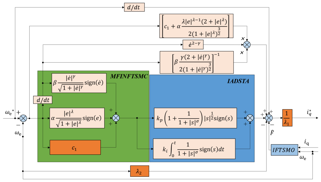
Combining Equations (8) and (47) yields the overall control law $i_q^{*}$ (as shown in Figure 1) for the novel ultra-local speed controller:

$$\begin{gathered} i_q^{*}={\displaystyle \frac{{\dot{\omega }}_e^{*}-{\lambda }_2{\omega }_e-F+u_c}{{\lambda }_1}} \\ ={\displaystyle \frac{1}{{\lambda }_1}}\left[\begin{array}{c}{\dot{\omega }}_e^{*}+\left[c_1+\alpha {\displaystyle \frac{\lambda |e{|}^{\lambda -1}(2+|e{|}^{\lambda })}{2(1+|e{|}^{\lambda }{)}^{\frac{3}{2}}}}\right]{\left[\beta {\displaystyle \frac{\gamma \left(2+|\dot{e}{|}^{\gamma }\right)}{2(1+|\dot{e}{|}^{\gamma }{)}^{\frac{3}{2}}}}\right]}^{-1}{\dot{e}}^{2-\gamma }\\ {+k}_p\left(1+{\displaystyle \frac{1}{1+|s{|}^{\sigma }}}\right)|s{|}^{{\displaystyle \frac{1}{2}}}\mathrm{sign}\left(s\right)+\\ k_i{\int }_0^t\hspace{1em}{\displaystyle \frac{1}{1+|s{|}^{\sigma }}}\mathrm{sign}\left(s\right)dt-{\lambda }_2{\omega }_e-F\end{array}\right] \end{gathered}$$

(48)

4. Design of IFTSMO

It follows from Equation (7) that the system control input is subject to an unknown disturbance $F$, extending $F$ as a state variable. For precise estimation of the composite unknown disturbance, an IFTSMO is constructed. Building upon Equation (7), the enhanced novel ultra-local model governing the speed loop is subsequently presented as follows:

$$\left\{\begin{array}{c}{\displaystyle \frac{d{\omega }_e}{dt}}={\lambda }_1{i}_q+{\lambda }_2{\omega }_e+F\hfill \\ {\displaystyle \frac{dF}{dt}}=\Gamma (t)\hfill \end{array}\right.$$

(49)

where $\Gamma \left(t\right)$ represents the time derivative of the unknown disturbance $F$. For the system described by Equation (49), an IFTSMO is designed, as shown in Equation (50):

$$\left\{\begin{array}{c}{\displaystyle \frac{d{\widehat{\omega }}_e}{dt}}={\lambda }_1{i}_q+{\lambda }_2{\widehat{\omega }}_e+\widehat{F}+u_{smo}\hfill \\ {\displaystyle \frac{d\widehat{F}}{dt}}=\epsilon \cdot u_{smo}\hfill \end{array}\right.$$

(50)

where ${\widehat{\omega }}_{\mathrm{e}}$ denotes the estimated electrical angular velocity; $\widehat{F}$ represents the real-time estimated value of the unknown disturbance in the system; $u_{\mathrm{s}\mathrm{m}\mathrm{o}}$ is the sliding mode control law; and $\epsilon >0$ is the observer gain. Combining Equations (49) and (50), the speed observation error equation is derived, as shown in Equation (51):

$$\left\{\begin{array}{c}{\dot{e}}_{\omega }={\lambda }_2{e}_{\omega }+e_f+u_{smo}\hfill \\ {\dot{e}}_f=\epsilon \cdot u_{smo}-\Gamma \left(t\right)\hfill \end{array}\right.$$

(51)

Note that the derivative of the disturbance, $\Gamma \left(t\right)$, is bounded as per Assumption 1 ($|\Gamma (t)|\le {\delta }_2$), where $e_{\omega }$ denotes the speed estimation error, defined as $e_{\omega }={\widehat{\omega }}_{\mathrm{e}}-{\omega }_{\mathrm{e}}$; and the variable $e_f$ corresponds to the error in observing the unknown disturbance, defined as $e_f=\widehat{F}-F$. For the IFTSMO, the sliding mode surface proposed in Equation (13) is adopted, as shown in Equation (52):

$$l=c_1{e}_{\omega }+\alpha {\displaystyle \frac{|e_{\omega }{|}^{\lambda }}{\sqrt{1+|e_{\omega }{|}^{\lambda }}}}sign\left(e_{\omega }\right)+\beta {\displaystyle \frac{|{\dot{e}}_{\omega }{|}^{\gamma }}{\sqrt{1+|{\dot{e}}_{\omega }{|}^{\gamma }}}}sign\left({\dot{e}}_{\omega }\right)$$

(52)

The sliding mode reaching law is adopted as shown in Equation (53):

$$\dot{l}=-Wsign\left(l\right)$$

(53)

where $W>0$.

Theorem 2.

Adopting Equation (52) as the sliding mode surface and Equation (53) as the sliding mode reaching law, the system will inevitably achieve a stable state in finite time when the parameter $W>0$.

Proof. 

Consider the following Lyapunov function given by Equation (54):

$$V_3={\displaystyle \frac{1}{2}}{l}^2$$

(54)

Differentiating Equation (54) with respect to time yields the following:

$$\begin{array}{c}{\dot{V}}_3=l\dot{l}\hfill \\ =l\left[-Wsign\left(l\right)\right]\hfill \\ =-W\left|l\right|\hfill \end{array}\le 0$$

(55)

When the parameter $W>0$, it can ensure that the system states reach the sliding mode surface in a short finite time. From Equations (53)–(55), the control law of the IFTSMO is derived as follows:

$$u_{smo}={\displaystyle \frac{c_1+\alpha \frac{\lambda |e_{\omega }{|}^{\lambda -1}(2+|e_{\omega }{|}^{\lambda })}{2(1+|e_{\omega }{|}^{\lambda }{)}^{\frac{3}{2}}}}{\beta \frac{\gamma \left(2+|{\dot{e}}_{\omega }{|}^{\gamma }\right)}{2(1+|{\dot{e}}_{\omega }{|}^{\gamma }{)}^{\frac{3}{2}}}}}{{\dot{e}}_{\omega }}^{2-\gamma }-{\lambda }_2{\dot{e}}_{\omega }+Wsign\left(l\right)$$

(56)

From Equations (50) and (56), $\widehat{F}$ can be obtained as follows:

$$\widehat{F}=\epsilon {\int }_0^t\hspace{1em}{\displaystyle \frac{c_1+\alpha \frac{\lambda |e_{\omega }{|}^{\lambda -1}(2+|e_{\omega }{|}^{\lambda })}{2(1+|e_{\omega }{|}^{\lambda }{)}^{\frac{3}{2}}}}{\beta \frac{\gamma \left(2+|{\dot{e}}_{\omega }{|}^{\gamma }\right)}{2(1+|{\dot{e}}_{\omega }{|}^{\gamma }{)}^{\frac{3}{2}}}}}{{\dot{e}}_{\omega }}^{2-\gamma }-{\lambda }_2{\dot{e}}_{\omega }+Wsign\left(l\right)dx$$

(57)

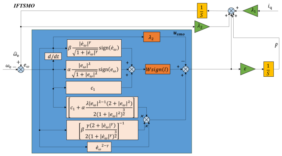
Substituting Equation (57) into Equation (50) yields the overall control law $i_q^{*}$ (as shown in Figure 2) of the controller:

$$\begin{gathered} i_q^{*}={\displaystyle \frac{{\dot{\widehat{\omega }}}_e^{*}-{\lambda }_2{\widehat{\omega }}_e-\widehat{F}+u_{smo}}{{\lambda }_1}} \\ ={\displaystyle \frac{1}{{\lambda }_1}}\left[\begin{array}{c}{\dot{\widehat{\omega }}}_e^{*}+\left[c_1+\alpha {\displaystyle \frac{\lambda |e{|}^{\lambda -1}(2+|e{|}^{\lambda })}{2(1+|e{|}^{\lambda }{)}^{\frac{3}{2}}}}\right]{\left[\beta {\displaystyle \frac{\gamma \left(2+|\dot{e}{|}^{\gamma }\right)}{2(1+|\dot{e}{|}^{\gamma }{)}^{\frac{3}{2}}}}\right]}^{-1}{\dot{e}}^{2-\gamma }\\ {+k}_p\left(1+{\displaystyle \frac{1}{1+|s{|}^{\sigma }}}\right)|s{|}^{{\displaystyle \frac{1}{2}}}\mathit{sign}\left(s\right)+\\ k_i{\int }_0^t\hspace{1em}{\displaystyle \frac{1}{1+|s{|}^{\sigma }}}\mathrm{sign}\left(s\right)dt-{\lambda }_2{\widehat{\omega }}_e-\widehat{F}\end{array}\right] \end{gathered}$$

(58)

□

5. Experimental Analysis

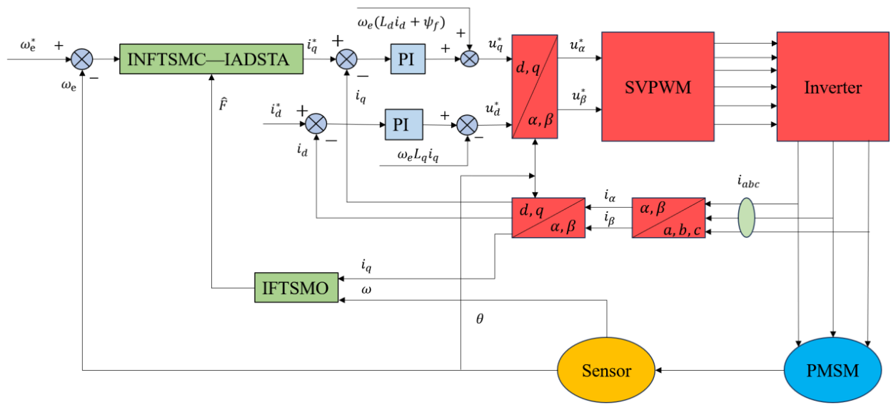
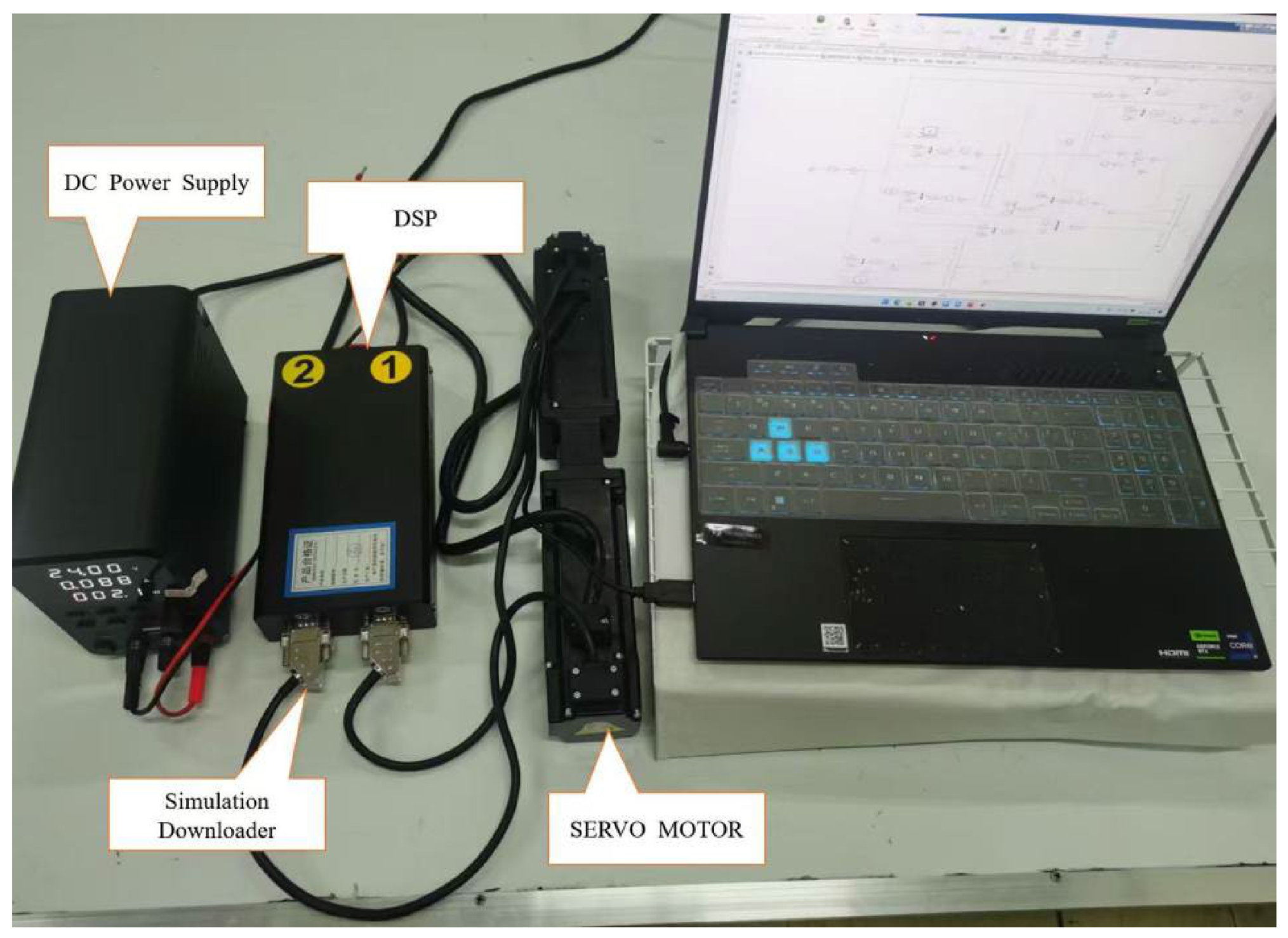
To validate the effectiveness and superiority of the proposed MFINFTSMC-IADSTA-IFTSMO controller, a physical back-to-back motor experimental platform was constructed based on the control block diagram shown in Figure 3, simulating the architecture of an agricultural UAV electromechanical system. The experimental setup, illustrated in Figure 4, employs the TMS320F28379D digital signal processor (DSP) as the core control unit to replicate the high-dynamic operating environment of an agricultural UAV propulsion system. For comparative analysis, five representative control strategies—namely SMC-STA, INFTSMC-STA, INFTSMC-IADSTA, MFINFTSMC-IADSTA-SMO, SMC [30], and the proposed MFINFTSMC-IADSTA-IFTSMO—were selected for evaluation under simulated agricultural UAV operational conditions. The detailed parameters of the PMSM and the tuned parameters of the five controllers are listed in

Table 1. Parameters of SPMSM.

Parameters	Numerical Value
Number of Pole Pairs	4
Stator Phase Resistance	0.1 Ω
Stator inductance (d-q axis)	1.9 × 10−4 H
Permanent Magnet Chain	0.0133 Wb
moment of inertia (mechanics)	4.03 × 10−4 kg·m2
Viscous Damping Coefficient	3.1136 × 10−4 N·m·s

and

Table 2. Controller parameters.

SMC-STA [28]	$c_1=8$; $k_p=2600$; $k_i=8000$
INFTSMC-STA [31]	$c_1=8$; $\alpha =7$; $\beta =3.8$; $\lambda =2.2\left(p=33, q=15\right);$ $\gamma =1.7\left(y=35, z=21\right); k_p=2500$; $k_i=9000$
INFTSMC-IADSTA	$c_1=8$; $\alpha =7; \beta =3.8; \lambda =2.2\left(p=33, q=15\right);$ $\gamma =1.7(y=35, z=21); k_p=4000; k_i=\mathrm{18,000};$ $\sigma =$40,000
MFINFTSMC-IADSTA-SMO [1]	$c_1=7$; $W=\mathrm{13,000}; \epsilon =-0.000005$
SMC [30]	${\eta }_1=10; {\eta }_2=0.003; p=5; q=7$; $\epsilon =\mathrm{15,000}$; $\lambda =10$
MFINFTSMC-IADSTA-IFTSMO	$c_1=8$; $\alpha =7; \beta =3.8;\lambda =2.2\left(p=33, q=15\right);$ $\gamma =1.7(y=35, z=21); W=\mathrm{13,000};$$\epsilon =-0.000005$

(Note: Reference [30] Control law: $i_q^{*}={\displaystyle \frac{-F+{\dot{\omega }}_e^{*}}{\alpha }}+{\displaystyle \frac{\epsilon \mathrm{s}\mathrm{g}\mathrm{n}(s)+\lambda s+\ddot{e}+{\eta }_2|e{|}^{p/q}\mathrm{s}\mathrm{g}\mathrm{n}(e)}{\alpha \cdot {\eta }_1}}$.

, respectively. A Space Vector Pulse Width Modulation (SVPWM) technique, with its switching frequency set to 10 kHz, is implemented in the vector control system. A low-pass filter with a cutoff frequency of 0.001 rad/s is used for signal conditioning, simulating the actual signal processing conditions in an agricultural UAV electronic control system.

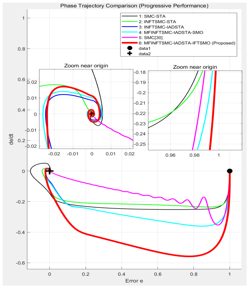
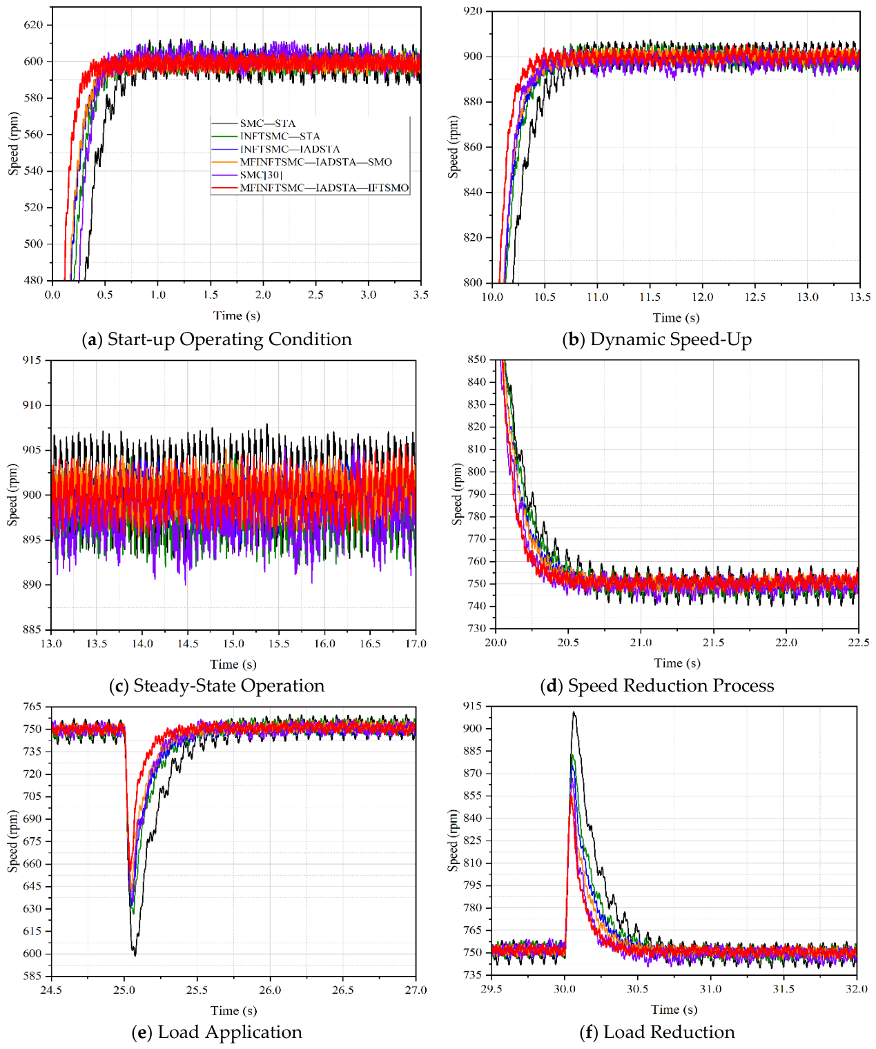
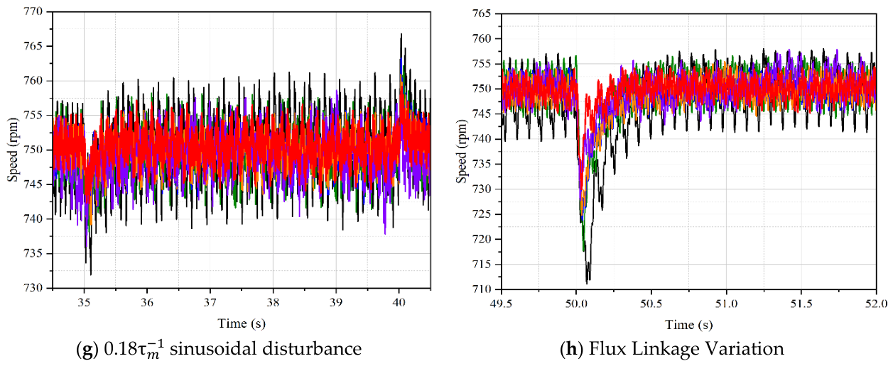
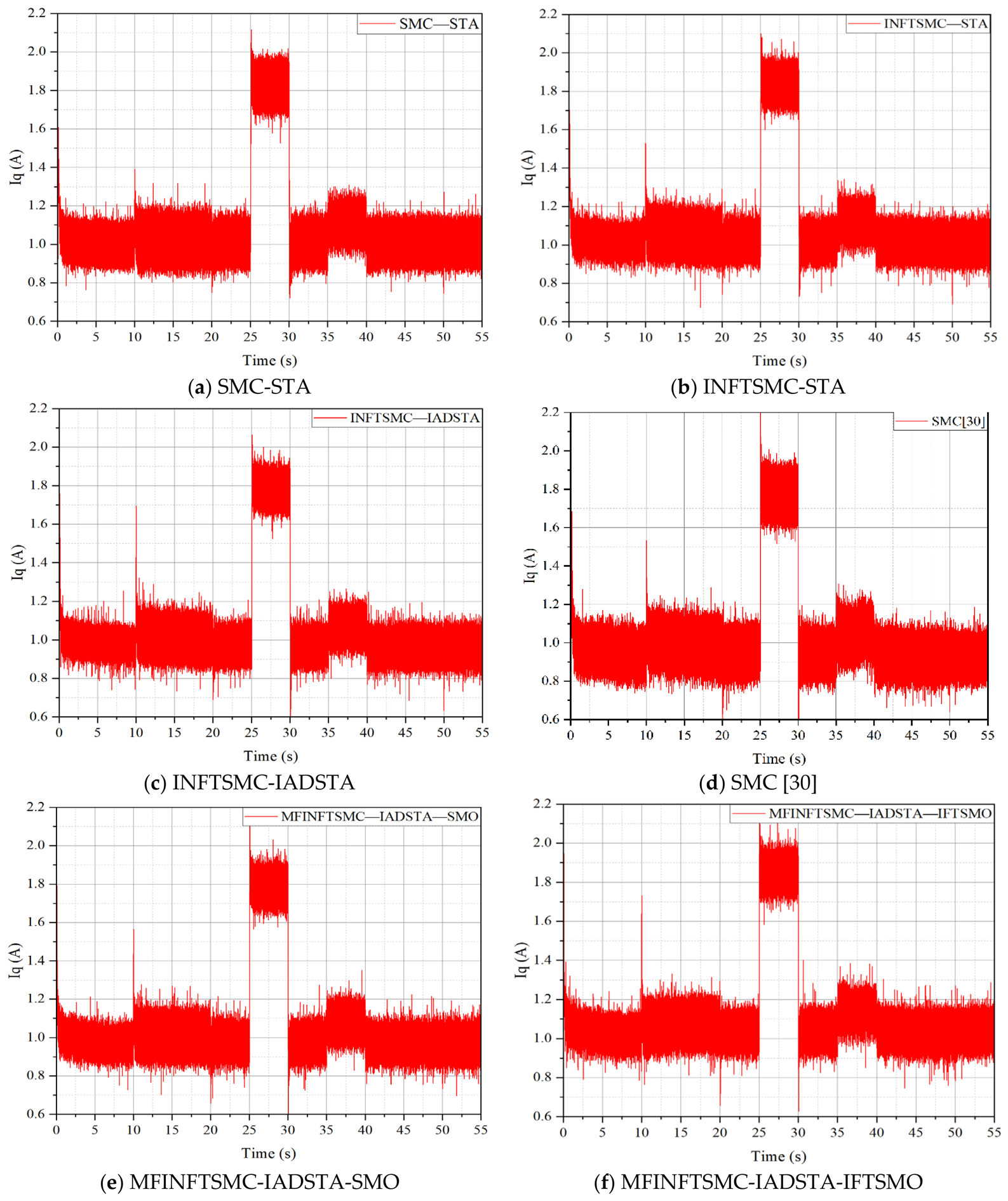
The experimental operating conditions are configured as follows: no-load start-up with the speed initially ramped up to 600 $\mathrm{r}\mathrm{p}\mathrm{m}$. At the 10 s and 20 s marks, the reference speed is set to 900 rpm and 750 rpm, respectively. Subsequently, a $0.1\mathrm{N}\cdot \mathrm{m}$ load torque is applied at 25 s and then removed at 30 s; the sinusoidal disturbance frequency is adjusted to 0.18${\mathsf{\tau }}_m^{-1}$ (where ${\mathsf{\tau }}_{\mathrm{m}}$ denotes the mechanical time constant) at 35 s. At 50 s, the flux linkage is adjusted upward to 1.3 of its initial value. Figure 5 shows the phase trajectory plots of different control algorithms. The speed waveforms and q-axis current waveforms are illustrated in Figure 6 and Figure 7, respectively.

Experimental Results and Performance Analysis

To comprehensively evaluate the performance of the proposed method under the high-dynamic and multi-disturbance conditions typical of agricultural UAV applications, comparative experiments were conducted between the MFINFTSMC-IADSTA-IFTSMO and four benchmark controllers: SMC-STA, INFTSMC-STA, INFTSMC-IADSTA, SMC [30], and MFINFTSMC-IADSTA-SMO. The results, presented in Figure 6 and

Table 3. A comparative assessment of different control strategies.

Control Strategies	Start-Up Convergence Time	Steady-State Error	Sinusoidal Disturbance	Flux Disturbance	Load Disturbance	Speed-Up Settling Time (600–900 rpm, s)
SMC-STA [28]	0.8	7	10	0.7	150	0.85
INFTSMC-STA [31]	0.7	6	8	0.65	128	0.75
INFTSMC-IADSTA	0.65	5	6	0.5	119	0.7
MFINFTSMC-IADSTA-SMO [1]	0.6	4	5	0.45	115	0.65
SMC [30]	0.65	5	6	0.4	117	0.55
MFINFTSMC-IADSTA-IFTSMO	0.35	3	4	0.3	96	0.5

, demonstrate that the proposed method achieves superior comprehensive performance across all test scenarios. To quantitatively evaluate the convergence performance of the proposed algorithms, a universally accepted industrial criterion is adopted in this paper: the convergence/settling time is defined as the total duration required for the actual motor speed to enter and stably remain within a ±2% error band of the target speed after a step change in the speed reference command.

During the start-up transient from standstill to 600 rpm, the proposed controller achieved the shortest start-up time of 0.35 s with a minimal fluctuation amplitude of 5 rpm and a smooth speed trajectory, significantly outperforming the SMC-STA controller, which exhibited the longest start-up time (0.8 s) and pronounced fluctuations (10 rpm). This performance advantage is attributed to the powerful driving capability of the INFTSM surface (Equation (13)) in the large-error region, facilitated by its nonlinear power terms and the dynamic gain adjustment of the IADSTA (Equation (20)), which balances rapid convergence with chattering suppression.

In the speed regulation tests, including acceleration (600 → 900 rpm) and deceleration (900 → 750 rpm), the proposed method demonstrated the fastest response, completing the transitions in 0.5 s and 0.6 s, respectively, without overshoot or oscillations. The IFTSMO (Equation (52)), designed based on the ultra-local model (Equation (7)), played a critical role by providing real-time, high-precision estimation of unknown disturbances for feedforward compensation. This observer–controller synergy, maintained through a homologous design logic, effectively mitigates the impact of model mismatches and inertial disturbances during dynamic transitions.

Under steady-state operation at 900 rpm, the proposed algorithm minimized the speed fluctuation to merely 3 rpm and eliminated high-frequency chattering. Such high-fidelity steady-state performance is achieved through a synergy between the IADSTA’s low-gain operation under small-error conditions and the intrinsic convergence smoothness of the INFTSMS design. The controller’s robustness was further validated under significant disturbances. When a load torque of 0.1 N·m was suddenly applied and removed, the proposed method exhibited the smallest speed deviation (96 rpm) and the fastest recovery time (<0.3 s), with no overshoot upon load release. This strong disturbance rejection capability is achieved through the rapid capture and compensation of sudden load changes by the IFTSMO, combined with the fast error suppression of the IADSTA.

The controller’s ability to handle complex, time-varying disturbances was confirmed under a sinusoidal disturbance with a frequency of 0.18 τ_m⁻¹; the controller limited speed oscillations to within 4 rpm—even when subjected to a significant parameter mismatch. An instantaneous rise in flux linkage to 1.3 of its rated value limited the fluctuation to 20 rpm. These results underscore the effectiveness of the model-free framework, which eliminates dependence on motor parameters, and the high-precision compensation capability of the IFTSMO for time-varying and parametric disturbances.

Compared with the SMC algorithm proposed in Ref. [30], the MFINFTSMC-IADSTA-IFTSMO control method proposed in this paper exhibits superior comprehensive performance under all test operating conditions.

During the dynamic transients of start-up, acceleration and deceleration, the proposed method achieves a faster response speed (0.3 s shorter than that of SMC [30]), and its dynamic fluctuation amplitude in steady-state operation outperforms that of SMC [30], which addresses the inherent problems of slow convergence and large dynamic error in traditional SMC. During steady-state operation, the proposed method effectively suppresses high-frequency chattering, with its steady-state speed ripple far lower than that of SMC [30], thus achieving higher control accuracy. Under severe disturbance conditions, including sudden load torque application and removal, sinusoidal time-varying disturbances, and parameter mismatch, the proposed method yields smaller speed deviation and faster recovery speed and possesses stronger disturbance rejection capability and robustness compared with SMC [30].

Based on Figure 6 and Figure 7, it can be seen that the control strategy proposed in this paper can maintain good q-axis current response under various disturbances, especially when applying load torque. Compared with SMC-STA and INFTSMC-STA, the current peak of the IADSTA based control strategy is the smallest, and at variable speeds, the current peak of MFINFTSMC-IADSTA-IFTSMO is the highest but does not exceed the current threshold, proving that its response speed is faster.

6. Conclusions

This paper addresses issues in the SPMSM of agricultural UAV electric control systems, such as parameter variations, unknown disturbances, and severe chattering in traditional sliding mode control. It proposes an MFINFTSMC-IADSTA-IFTSMO. Experimental results demonstrate that this method successfully achieves the following objectives:

(1) Fast convergence and non-singularity: The designed improved non-singular fast terminal sliding surface, by integrating error power terms and dynamic damping feedback, completely eliminates the singularity of traditional terminal sliding mode while achieving fixed-time convergence of the system. This significantly enhances dynamic response speed and transient smoothness.

(2) Strong robustness and high-precision control: The improved adaptive super-twisting reaching law, through the dynamic association of gains and sliding mode states, effectively resolves the conflict between convergence speed and chattering suppression. Combined with the real-time feedforward compensation of disturbances by the IFTSMO constructed within a model-free framework, it ensures the system’s robustness and high steady-state accuracy under parameter variations and external disturbances.

Comprehensive experimental studies show that the proposed MFINFTSMC-IADSTA-IFTSMO strategy significantly outperforms existing advanced methods in terms of dynamic response, precision in steady-state operation, and ability to attenuate disturbances. Specifically, under sudden load conditions, its speed drop is reduced by approximately 85% compared to traditional methods, with steady-state fluctuations attenuated by over 75%. Additionally, the system exhibits excellent stability under time-varying sinusoidal disturbances and parameter variations. Future research could focus on extending this method to broader industrial applications, such as sensorless control in agricultural UAV electric control systems.

References

1. Zhang, L.; Tao, R.; Li, X. Model-Free Adaptive Second Order Sliding Mode Control for PMSM in Electric Traction Systems Based on Terminal Attractor. IEEE Trans. Power Electron. 2026, 41, 11973–11984. [Google Scholar] [CrossRef]
2. Zhu, B.; Liao, W.; She, X.; An, J. High Reliability Multi-Input Converter with Low Input Current Ripple Based on SEPIC for Solar-Powered Unmanned Aerial Vehicle. IEEE Trans. Consum. Electron. 2026, early access. [Google Scholar] [CrossRef]
3. Ma, X.; Zhang, L.; Xu, Y.; Bai, J. Model-Free Control of Permanent Magnet Synchronous Motors with Improved Terminal Sliding Mode Based on a Modified Exponential Reaching Law. Control Eng. Pract. 2026, 166, 106630. [Google Scholar] [CrossRef]
4. Hu, M.; Zhang, L.; Tao, R.; Wang, P.; Gu, Y.; Ullah, Z. Nonlinear Integral Sliding Mode Control of SPMSMs Using a Dual-Layer Adaptive Super-Twisting Algorithm. Ain Shams Eng. J. 2026, 17, 103948. [Google Scholar] [CrossRef]
5. Khanh, P.Q.; Anh, H.P.H. Advanced PMSM Speed Control Using Fuzzy PI Method for Hybrid Power Control Technique. Ain Shams Eng. J. 2023, 14, 102222. [Google Scholar] [CrossRef]
6. Zhang, L.; Tao, R.; Bai, J.; Zeng, D. An Improved Sliding Mode Model Reference Adaptive System Observer for PMSM Applications. Expert Syst. Appl. 2024, 250, 123907. [Google Scholar] [CrossRef]
7. Zwerger, T.; Mercorelli, P. Noninteracting Optimal and Adaptive Torque Control Using an Online Parameter Estimation with Help of Polynomials in EKF for a PMSM. ISA Trans. 2025, 158, 452–467. [Google Scholar] [CrossRef]
8. Li, F.; Liu, Z.; Jiang, B. Adaptive Finite-Time Fuzzy Fractional Sliding Mode Control for Uncertain QUAV with Actuator Faults and Slung Load. IEEE Trans. Aerosp. Electron. Syst. 2024, 61, 3046–3058. [Google Scholar] [CrossRef]
9. Li, F.; Liu, Z.; Zhao, X. Prescribed-Time Tracking Control for a QUAV with a Cable-Suspended Payload and Asymmetric Partial Time-Interval Output Constraints. J. Frankl. Inst. 2025, 362, 107515. [Google Scholar] [CrossRef]
10. Mathew, K.K.; Abraham, D.M.; Harish, A. Speed Regulation of PMSM Drive in Electric Vehicle Applications with Sliding Mode Controller Based on Harris Hawks Optimization. e-Prime-Adv. Electr. Eng. Electron. Energy 2024, 9, 100643. [Google Scholar] [CrossRef]
11. Li, K.; Ding, J.; Sun, X.; Tian, X. Overview of Sliding Mode Control Technology for Permanent Magnet Synchronous Motor System. IEEE Access 2024, 12, 71685–71704. [Google Scholar] [CrossRef]
12. Liu, H. Fixed-Time Non-Singular Terminal Sliding Mode Control for PMSM Drive Systems. J. Power Electron. 2024, 24, 258–268. [Google Scholar] [CrossRef]
13. Jia, N.; Zhao, K.; Lv, Y.; Li, X. Non-Singular Fast Terminal Sliding Mode Control Torsional Vibration Suppression for PM Synchronous Transmission System of EVs. Prog. Electromagn. Res. M 2023, 122, 63–72. [Google Scholar] [CrossRef]
14. Zhang, L.; Tao, R.; Zhang, Z.-X.; Chien, Y.-R.; Bai, J. PMSM Non-Singular Fast Terminal Sliding Mode Control with Disturbance Compensation. Inf. Sci. 2023, 642, 119040. [Google Scholar] [CrossRef]
15. Xu, Q.; Jiang, D.; Wang, Y.; Zhang, X.; Liu, J.; Chen, Y. Variable-Step Close-Loop Angle Compensation Method of PMSM Rotor Position Estimation Based on Super-Twisting Sliding-Mode Observer Using Tangent Reaching Law. Energy Rep. 2023, 9, 356–361. [Google Scholar] [CrossRef]
16. Zheng, C.; Qin, X.; Chen, G. Sliding Mode Control of PMSM Control Based on Novel Exponential Reaching Law. J. Phys. Conf. Ser. 2023, 2503, 012085. [Google Scholar] [CrossRef]
17. Nan, Y.; Wang, L.; Qi, M.; Li, Z. Design of Variable Boundary Layer Sliding Mode Observer for Permanent Magnet Synchronous Motor Based on Fuzzy Control. Prog. Electromagn. Res. C 2025, 154, 119–129. [Google Scholar] [CrossRef]
18. Lv, D.; Zhang, C.; Zhao, W. A Robust and Chattering-Free Control Method for the Speed of PMSM Drive Systems Based on New Adaptive Reaching Law. Electr. Eng. 2025, 107, 13947–13958. [Google Scholar] [CrossRef]
19. Mencou, S.; Yakhlef, M.B.; Tazi, E.B. Advanced Control of Induction Motors (2019–2025): A Comprehensive Review of Strategies, Algorithms and Sensorless Techniques. e-Prime-Adv. Electr. Eng. Electron. Energy 2025, 14, 101098. [Google Scholar] [CrossRef]
20. Li, S.; Li, H.; Wang, H.; Yang, C.; Gui, J.; Fu, R. Sliding Mode Active Disturbance Rejection Control of Permanent Magnet Synchronous Motor Based on Improved Genetic Algorithm. Actuators 2023, 12, 209. [Google Scholar] [CrossRef]
21. Hu, M.; Ahn, H.; Chung, Y.; You, K. Speed Regulation for PMSM with Super-Twisting Sliding-Mode Controller via Disturbance Observer. Mathematics 2023, 11, 1618. [Google Scholar] [CrossRef]
22. Wang, G.; Zhang, H. A Second-Order Sliding Mode Observer Optimized by Neural Network for Speed and Position Estimation of PMSMs. J. Electr. Eng. Technol. 2022, 17, 415–423. [Google Scholar] [CrossRef]
23. Bıçak, A.; Gelen, A. Modified Super-Twisting Algorithm-Based Model Reference Adaptive Observer for Sensorless Control of the Interior Permanent-Magnet Synchronous Motor in Electric Vehicles. Machines 2023, 11, 871. [Google Scholar] [CrossRef]
24. Wang, X.; Li, X.; Zhang, D.; Wu, T. An Improved Global Fast Terminal High-Order Sliding Mode Control Strategy Based on Novel Reaching Law for Improving PMLSM Dynamic Performance. Energy Rep. 2023, 9, 829–838. [Google Scholar] [CrossRef]
25. Xu, L.; Chen, G.; Li, Q. Cascaded Speed and Current Model of PMSM with Ultra-Local Model-Free Predictive Control. IET Electr. Power Appl. 2021, 15, 1424–1437. [Google Scholar] [CrossRef]
26. Hua, C.; Shi, D.; Chen, X.; Gao, G. Ultra-Local Model-Based Adaptive Enhanced Model-Free Control for PMSM Speed Regulation. Machines 2025, 13, 541. [Google Scholar] [CrossRef]
27. Hagras, A.A.; Azab, A.; Zaid, S. Model-Free Nonsingular Fast Terminal Sliding Mode Control of a Permanent Magnet Synchronous Motor. Acta Polytech. Hung. 2024, 21, 283–305. [Google Scholar] [CrossRef]
28. Zhang, H.; Ran, P.; Zhang, Z. PMSM Sensorless Control Based on Super-Twisting Algorithm Sliding Mode Observer with the IAORLS Parameter Estimations. Sci. Rep. 2025, 15, 22386. [Google Scholar] [CrossRef]
29. Chen, H. PMSM Adaptive Sliding Mode Controller Based on Improved Linear Dead Time Compensation. Actuators 2022, 11, 267. [Google Scholar] [CrossRef]
30. Zhao, K. Model-Free Fast Integral Terminal Sliding-Mode Control Method Based on Improved Fast Terminal Sliding-Mode Observer for PMSM with Unknown Disturbances. ISA Trans. 2023, 143, 572–581. [Google Scholar] [CrossRef] [PubMed]
31. Yu, X.; Feng, Y.; Man, Z. Terminal Sliding Mode Control–An Overview. IEEE Open J. Ind. Electron. Soc. 2021, 2, 36–52. [Google Scholar] [CrossRef]
Figure 1. Control block diagram of MFINFTSMC-IADSTA.
Symmetry 18 00678 g001
Figure 2. Structure block diagram of IFTSMO.
Symmetry 18 00678 g002
Figure 3. MFINFTSMC-IADSTA-IFTSMO control block diagram.
Symmetry 18 00678 g003
Figure 4. Experimental platform.
Symmetry 18 00678 g004
Figure 5. Phase trajectory plots of different control algorithms.
Symmetry 18 00678 g005
Figure 6. Speed performance experiments.
Symmetry 18 00678 g006aSymmetry 18 00678 g006b
Figure 7. q-Axis current performance experiments.
Symmetry 18 00678 g007