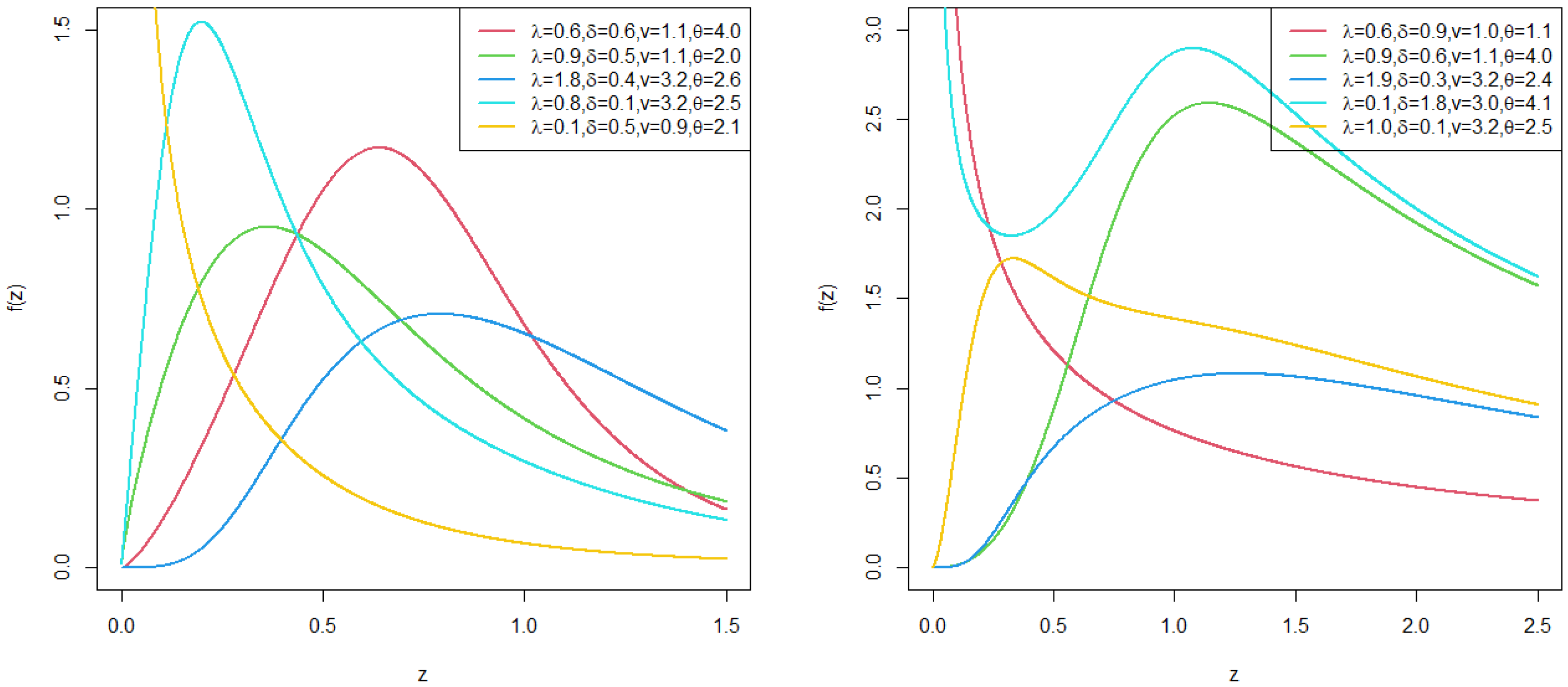
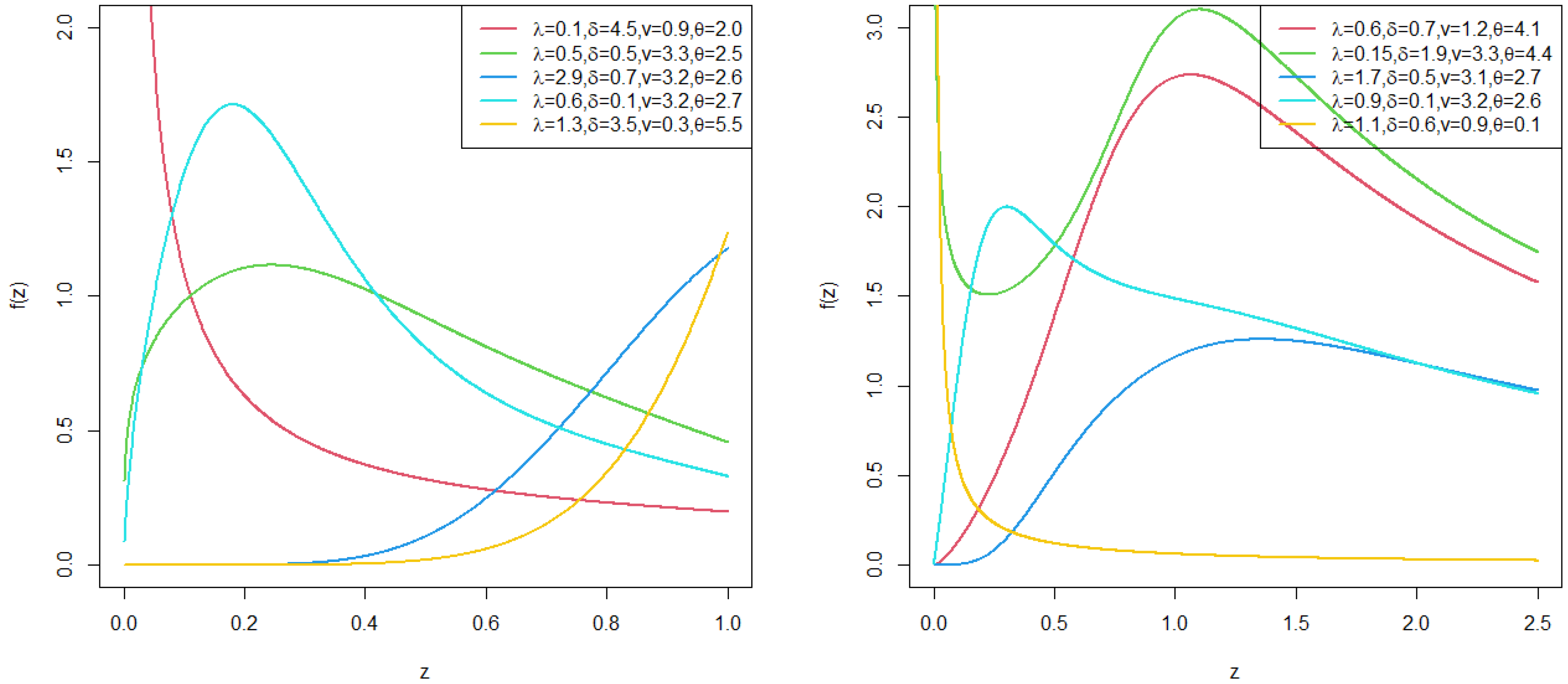
Exploring the New Exponentiated Harris-G Family of Distributions and Its Applications


Abstract
1. Introduction
2. The Proposed Family
Tail Behavior Analysis
- If , the tail of the proposed model is heavier than that of the subfamily (and heavier than the baseline if ).
- If , the tail is lighter.
3. Some Statistical Properties
3.1. Quantile Function
3.2. Series Expansion
4. Particular Cases
4.1. ExpH-LLoG Distribution
4.2. ExpH-W Distribution
5. Additional Statistical Properties
5.1. Distribution of Order Statistics
5.2. Uncertainty Measure
5.3. Moments
5.3.1. Moments and Moment Generating Functions
5.3.2. Conditional Moments
6. Parameter Estimation
ML Estimation
7. Simulation Design and Results
8. Applications
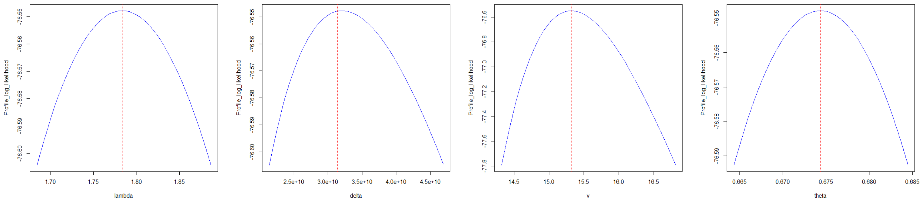
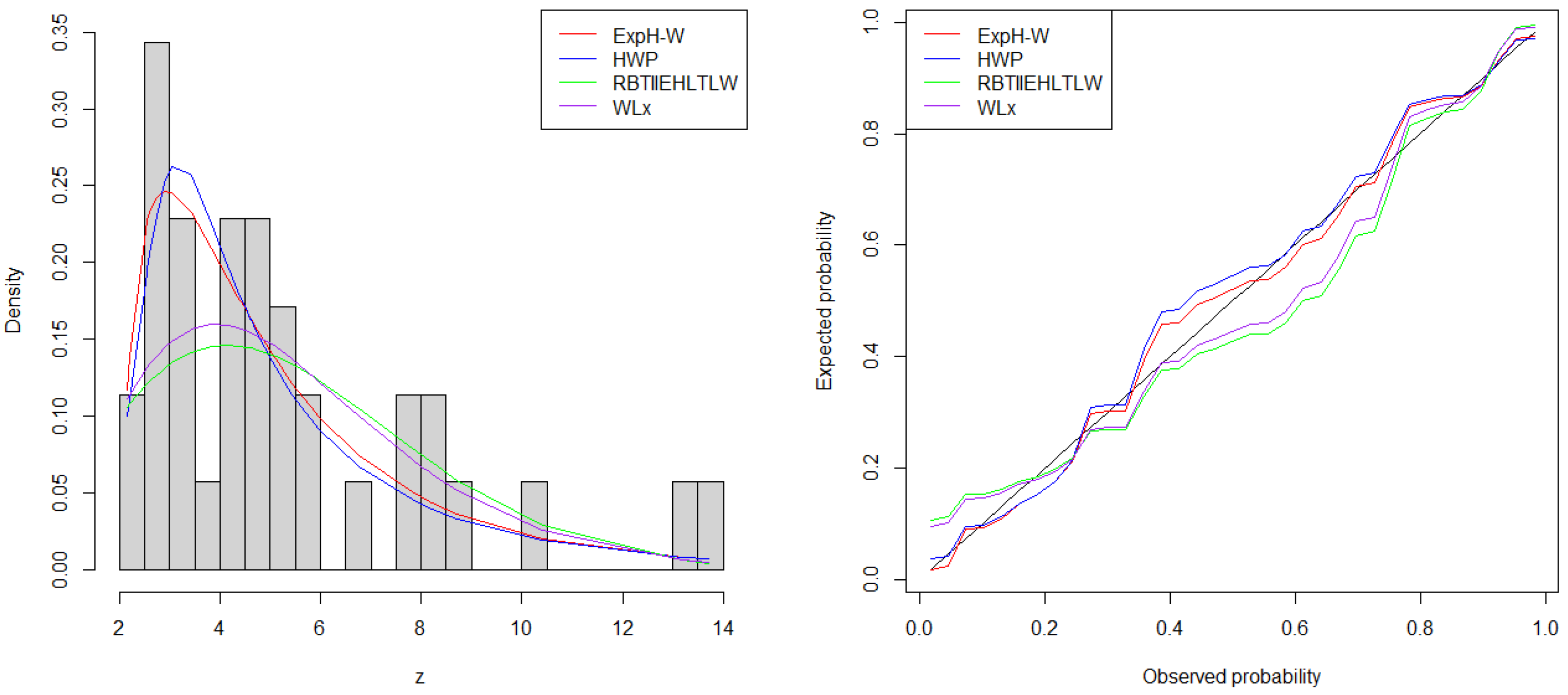
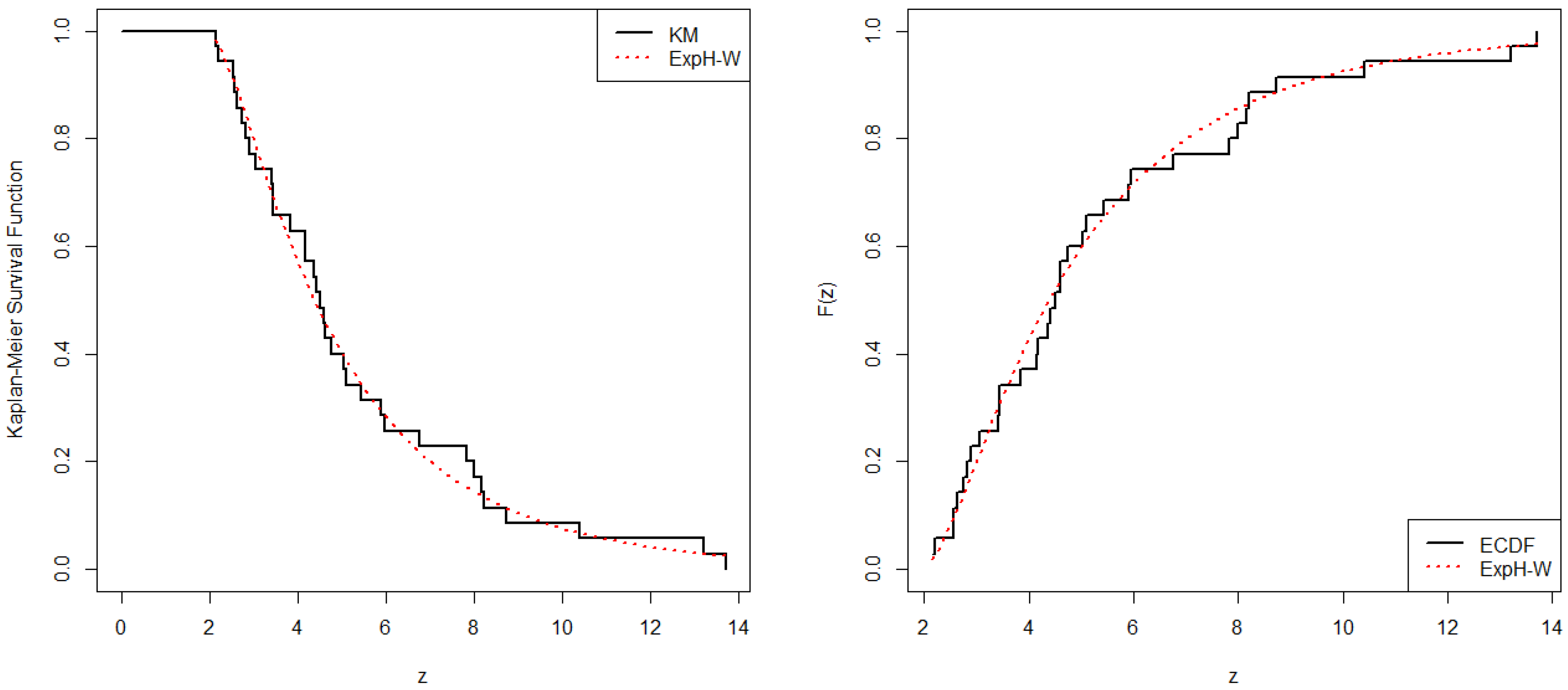
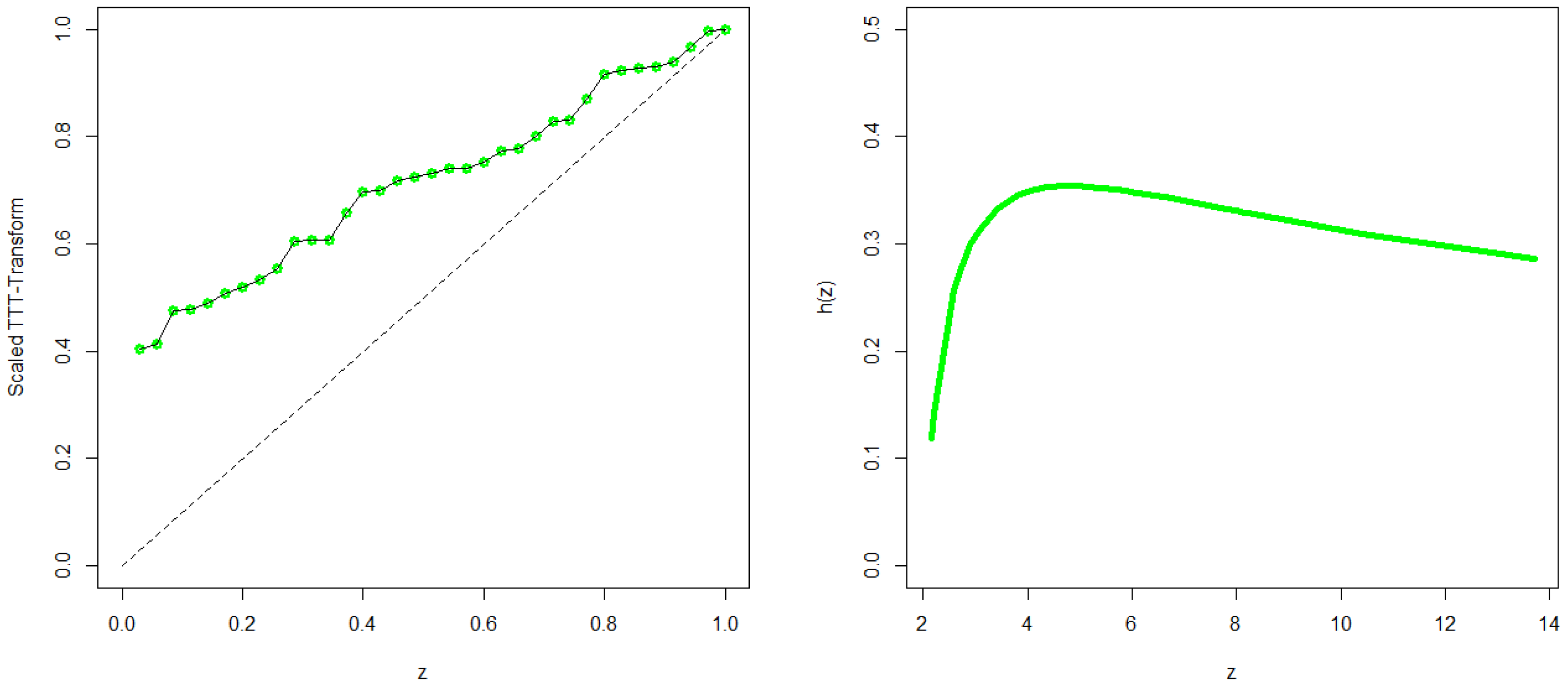
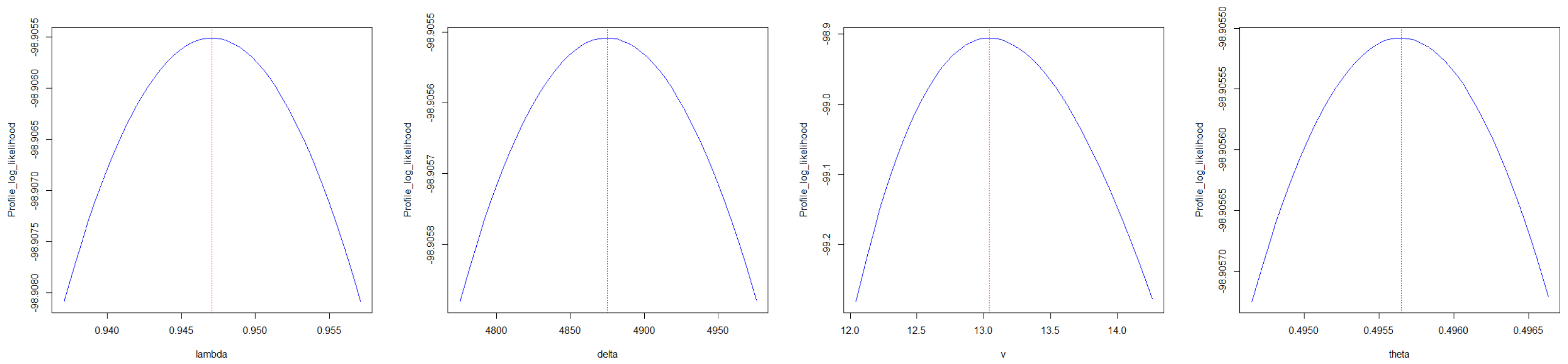
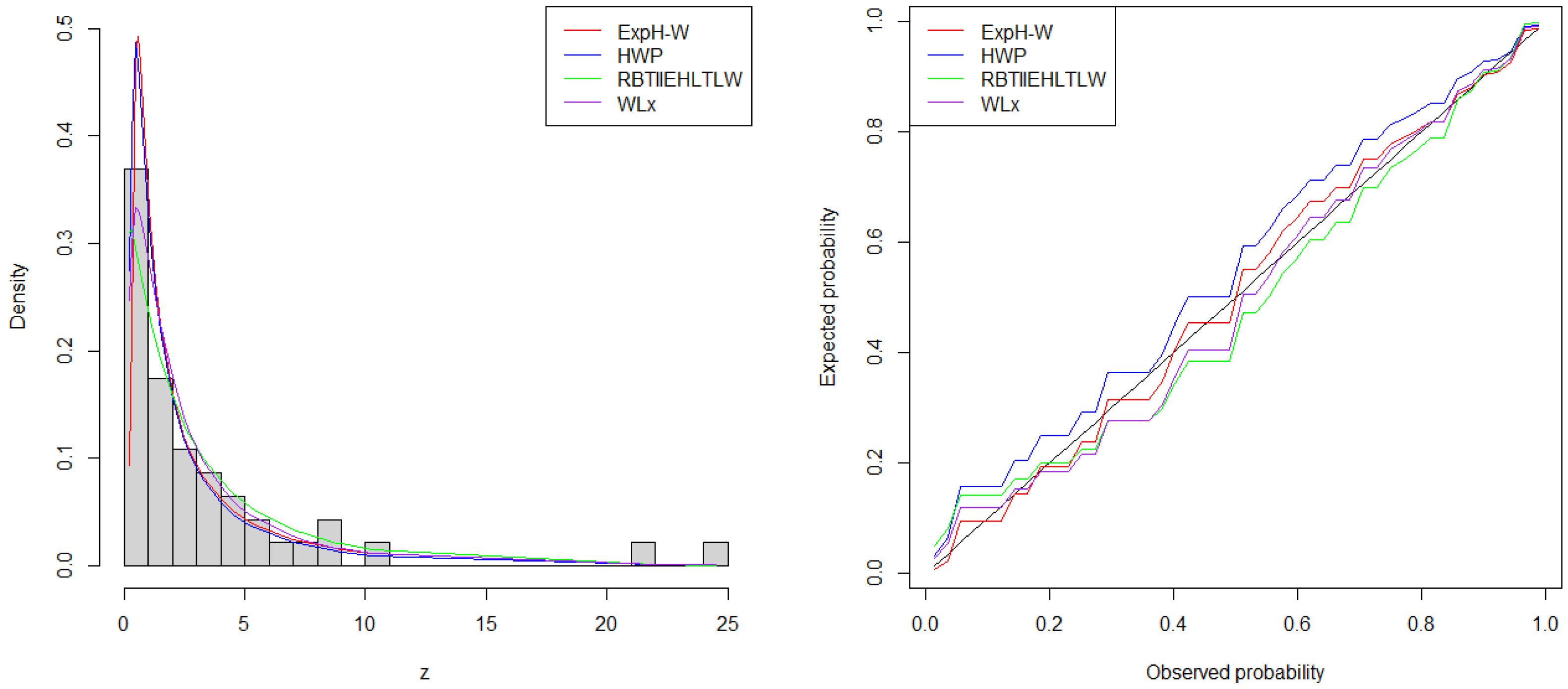
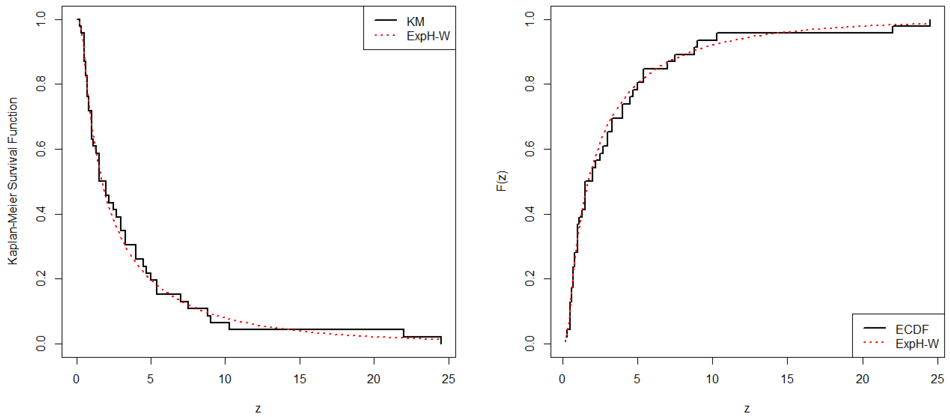
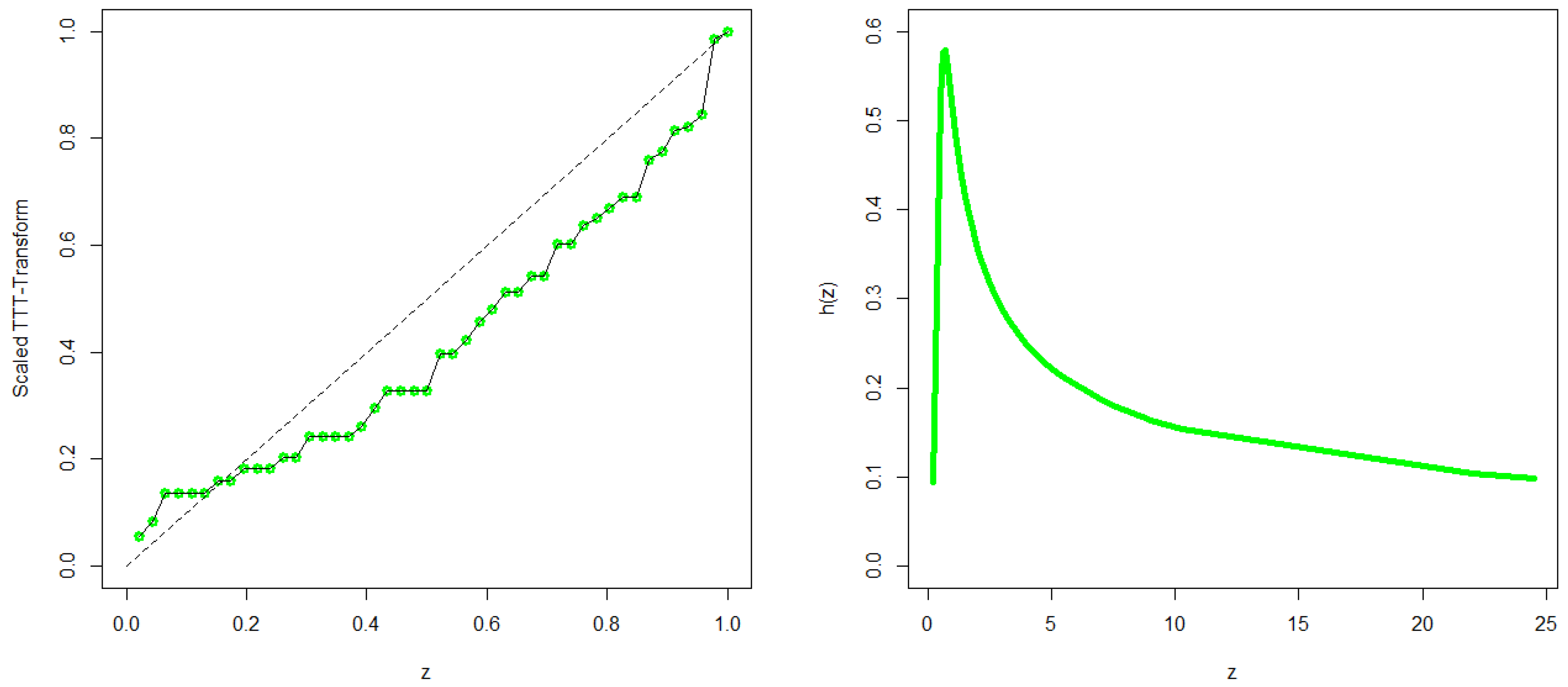
8.1. Growth Hormone Data
8.2. Repair Time Data
9. Conclusions
Supplementary Materials
Author Contributions
Funding
Data Availability Statement
Conflicts of Interest
References
- Pearson, K. Contributions to the mathematical theory of evolution II: Skew variation in homogeneous material. Philos. Trans. R. Soc. Lond. 1895, 186, 343–414. [Google Scholar] [CrossRef]
- Hastings, J.C.; Mosteller, F.; Tukey, J.W.; Windsor, C. Low moments for small samples: A comparative study of order statistics. Ann. Stat. 1947, 18, 413–426. [Google Scholar] [CrossRef]
- Tukey, J.W. The Practical Relationship Between the Common Transformations of Percentages of Counts and Amounts; Technical Report 36; Statistical Techniques Research Group, Princeton University: Princeton, NJ, USA, 1960. [Google Scholar]
- Johnson, N.L. Systems of frequency curves generated by methods of translation. Biometrika 1949, 36, 149–176. [Google Scholar] [CrossRef]
- Topp, C.W.; Leone, F.C. A family of J-shaped frequency functions. J. Am. Stat. Assoc. 1955, 50, 209–219. [Google Scholar] [CrossRef]
- Azzalini, A. A class of distributions which includes the normal ones. Scand. J. Stat. 1985, 12, 171–178. [Google Scholar]
- Azzalini, A. Further results on a class of distributions which includes the normal ones. Statistica 1986, 46, 199–208. [Google Scholar]
- Mudholkar, G.S.; Srivastava, D.K. Exponentiated Weibull family for analyzing bathtub failure-rate data. IEEE Trans. Reliab. 1993, 42, 299–302. [Google Scholar] [CrossRef]
- Eugene, N.; Lee, C.; Famoye, F. The beta-normal distribution and its applications. Commun. Stat. Theory Methods 2002, 31, 497–512. [Google Scholar] [CrossRef]
- Alzaatreh, A.; Lee, C.; Famoye, F. A new method for generating families of continuous distributions. Metron 2013, 71, 63–79. [Google Scholar] [CrossRef]
- Cooray, K.; Ananda, M.M.A. Modeling actuarial data with a composite lognormal-Pareto model. Scand. Actuar. J. 2005, 5, 321–334. [Google Scholar] [CrossRef]
- Marshall, A.W.; Olkin, I. A new method for adding parameters to a family of distributions with application to the exponential and Weibull families. Biometrika 1997, 84, 641–652. [Google Scholar] [CrossRef]
- Gupta, R.C.; Gupta, P.L.; Gupta, R.D. Modeling failure time data by Lehmann alternatives. Commun. Stat. Theory Methods 1998, 27, 887–904. [Google Scholar] [CrossRef]
- Aly, E.; Benkherouf, L. A new family of distributions based on probability generating functions. Sankhya B 2011, 73, 70–80. [Google Scholar] [CrossRef]
- Shannon, C.E. A mathematical theory of communication. Bell Syst. Tech. J. 1948, 27, 379–423. [Google Scholar] [CrossRef]
- Rényi, A. On Measures of Entropy and Information. In Proceedings of the Fourth Berkeley Symposium on Mathematical Statistics and Probability, Berkeley, CA, USA, 20 June–30 July 1961; Volume 4, pp. 547–562. [Google Scholar]
- Charumbira, W.F.; Oluyede, B.; Chipepa, F. A new generalized gamma type II exponentiated half logistic-Topp-Leone-G family of distributions with applications. Electron. J. Appl. Stat. Anal. 2024, 17, 676–702. [Google Scholar]
- Tahir, M.H.; Zubair, M.; Mansoor, M.; Cordeiro, G.M.; Alizadeh, M.; Hamedani, G. A new Weibull-G family of distributions. Hacet. J. Math. Stat. 2016, 45, 629–647. [Google Scholar] [CrossRef]
- Afify, A.Z.; Alizadeh, M.; Zayed, M.; Ramires, T.G.; Louzada, F. The odd log-logistic exponentiated Weibull distribution: Regression modeling, properties, and applications. Iran. J. Sci. Technol. 2018, 42, 2273–2288. [Google Scholar] [CrossRef]
- Chipepa, F.; Chamunorwa, S.; Oluyede, B.; Makubate, B.; Zidana, C. The exponentiated half logistic-generalized-G power series class of distributions: Properties and applications. J. Probab. Stat. Sci. 2022, 20, 21–40. [Google Scholar]
- Korkmaz, M.C.; Yousof, H.M.; Hamedani, G.G. The exponential Lindley odd log-logistic-G family: Properties, characterizations and applications. J. Stat. Theory Appl. 2018, 17, 554–571. [Google Scholar] [CrossRef]
- Charumbira, W.F.; Oluyede, B.; Chipepa, F.; Gabaitiri, L. The Harris-G power series class of distributions with applications. Int. J. Math. Oper. Res. 2024, 29, 234–257. [Google Scholar] [CrossRef]
- Cordeiro, G.M.; De Castro, M. A new family of generalized distributions. J. Stat. Comput. Simul. 2011, 81, 883–898. [Google Scholar] [CrossRef]
- Alizadeh, M.; Bagheri, S.F.; Bahrami, S.E.; Ghobadi, S.; Nadarajah, S. Exponentiated power Lindley power series class of distributions: Theory and applications. Commun. Stat. Simul. Comput. 2017, 47, 2499–2531. [Google Scholar] [CrossRef]
- Tlhaloganyang, B.P.; Sengweni, W.; Oluyede, B. The gamma odd Burr X-G family of distributions with applications. Pak. J. Stat. Oper. Res. 2022, 18, 721–746. [Google Scholar] [CrossRef]



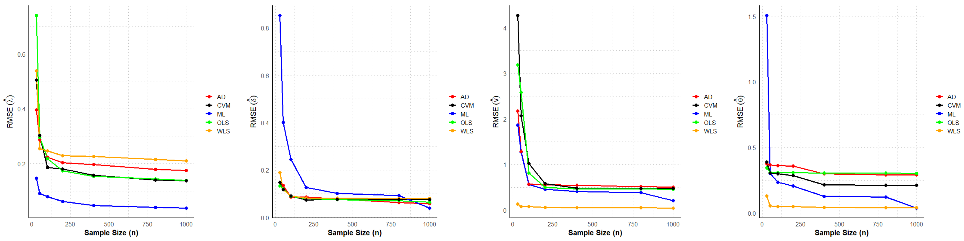
| Parameter | m | ML | AD | RMSE OLS | WLS | CVM | ML | AD | Abias OLS | WLS | CVM |
|---|---|---|---|---|---|---|---|---|---|---|---|
| 30 | 0.1468 (1) | 0.3958 (2) | 0.7406 (5) | 0.5383 (4) | 0.5049 (3) | 0.0803 (1) | 0.2222 (2) | 0.3588 (5) | 0.2366 (3) | 0.3004 (4) | |
| 30 | 0.8536 (5) | 0.1492 (3) | 0.1330 (1) | 0.1885 (4) | 0.1484 (2) | 0.4949 (5) | −0.0485 (2) | −0.0613 (3) | 0.0290 (1) | −0.0914 (4) | |
| v | 30 | 1.8633 (2) | 2.1753 (3) | 3.1832 (4) | 0.1331 (1) | 4.2749 (5) | 0.7945 (2) | 0.8512 (3) | 1.7417 (4) | 0.0869 (1) | 2.1626 (5) |
| 30 | 1.5071 (5) | 0.3767 (3) | 0.3455 (2) | 0.1307 (1) | 0.3882 (4) | 0.3701 (4) | −0.3730 (5) | −0.2690 (3) | −0.0242 (1) | −0.2616 (2) | |
| Sum of Ranks | 13 | 11 | 12 | 10 | 14 | 12 | 12 | 15 | 6 | 15 | |
| 50 | 0.0915 (1) | 0.2869 (3) | 0.2962 (4) | 0.2542 (2) | 0.3027 (5) | 0.0610 (1) | 0.2063 (3) | 0.1973 (2) | 0.2272 (5) | 0.2184 (4) | |
| 50 | 0.4006 (5) | 0.1350 (4) | 0.1203 (3) | 0.1172 (2) | 0.1171 (1) | 0.4747 (5) | 0.0403 (3) | −0.0298 (2) | 0.0282 (1) | −0.0573 (4) | |
| v | 50 | 1.2714 (2) | 1.2825 (3) | 2.5839 (5) | 0.0759 (1) | 2.0697 (4) | 0.4588 (2) | 0.4797 (3) | 1.1085 (5) | 0.0734 (1) | 1.0397 (4) |
| 50 | 0.3013 (2) | 0.3657 (5) | 0.3120 (4) | 0.0561 (1) | 0.3047 (3) | 0.2305 (2) | 0.3620 (5) | −0.2484 (4) | −0.0233 (1) | −0.2318 (3) | |
| Sum of Ranks | 14 | 13 | 15 | 6 | 12 | 10 | 14 | 13 | 8 | 15 | |
| 100 | 0.0798 (1) | 0.2238 (4) | 0.2185 (3) | 0.2470 (5) | 0.1858 (2) | 0.0576 (1) | 0.1955 (4) | 0.1640 (3) | 0.2126 (5) | 0.1562 (2) | |
| 100 | 0.2455 (5) | 0.0861 (1) | 0.0892 (2) | 0.0902 (3) | 0.0916 (4) | 0.4441 (5) | 0.0333 (3) | 0.0161 (1) | 0.0238 (2) | −0.0596 (4) | |
| v | 100 | 0.5649 (2) | 0.5715 (3) | 0.8145 (4) | 0.0736 (1) | 1.0229 (5) | 0.1156 (2) | −0.5582 (5) | 0.1260 (3) | −0.0672 (1) | 0.2277 (4) |
| 100 | 0.2335 (2) | 0.3614 (5) | 0.3070 (4) | 0.0491 (1) | 0.2992 (3) | 0.1007 (2) | −0.3485 (5) | −0.2699 (3) | −0.0356 (1) | −0.2604 (4) | |
| Sum of Ranks | 10 | 13 | 13 | 10 | 14 | 10 | 17 | 10 | 9 | 14 | |
| 200 | 0.0617 (1) | 0.2033 (4) | 0.1738 (2) | 0.2284 (5) | 0.1800 (3) | 0.0481 (1) | 0.1826 (4) | 0.1461 (2) | 0.2107 (5) | 0.1526 (3) | |
| 200 | 0.1270 (5) | 0.0854 (4) | 0.0793 (2) | 0.0811 (3) | 0.0744 (1) | 0.3825 (5) | 0.0332 (3) | 0.0173 (1) | 0.0244 (2) | 0.0533 (4) | |
| v | 200 | 0.4547 (2) | 0.5511 (4) | 0.4988 (3) | 0.0594 (1) | 0.5734 (5) | 0.1056 (2) | −0.5413 (5) | −0.1212 (3) | −0.0589 (1) | −0.1850 (4) |
| 200 | 0.2067 (2) | 0.3576 (5) | 0.3065 (4) | 0.0483 (1) | 0.2852 (3) | 0.0219 (1) | −0.3333 (5) | −0.2812 (4) | −0.0371 (2) | −0.2554 (3) | |
| Sum of Ranks | 10 | 17 | 11 | 10 | 12 | 9 | 17 | 10 | 10 | 14 | |
| 400 | 0.0476 (1) | 0.1970 (4) | 0.1539 (2) | 0.2257 (5) | 0.1578 (3) | 0.0364 (1) | 0.1856 (4) | 0.1369 (2) | 0.2068 (5) | 0.1396 (3) | |
| 400 | 0.1022 (5) | 0.0778 (3) | 0.0753 (1) | 0.0809 (4) | 0.0763 (2) | 0.0432 (4) | 0.0324 (3) | 0.0140 (1) | 0.0233 (2) | 0.0530 (5) | |
| v | 400 | 0.4051 (2) | 0.5437 (5) | 0.4678 (3) | 0.0523 (1) | 0.4799 (4) | −0.0858 (2) | −0.3589 (5) | −0.1167 (3) | −0.0504 (1) | −0.3279 (4) |
| 400 | 0.1272 (2) | 0.3001 (4) | 0.3060 (5) | 0.0424 (1) | 0.2162 (3) | 0.0216 (1) | −0.2433 (4) | −0.2992 (5) | −0.0399 (2) | −0.1973 (3) | |
| Sum of Ranks | 10 | 16 | 11 | 11 | 12 | 8 | 16 | 11 | 10 | 15 | |
| 800 | 0.0401 (1) | 0.1785 (4) | 0.1438 (3) | 0.2155 (5) | 0.1399 (2) | 0.0361 (1) | 0.1727 (4) | 0.1329 (3) | 0.2093 (5) | 0.1320 (2) | |
| 800 | 0.0918 (5) | 0.0627 (1) | 0.0707 (2) | 0.0803 (4) | 0.0760 (3) | 0.0230 (4) | 0.0271 (3) | 0.0119 (1) | 0.0175 (2) | 0.0534 (5) | |
| v | 800 | 0.3842 (2) | 0.5152 (5) | 0.4643 (3) | 0.0466 (1) | 0.4745 (4) | 0.0335 (1) | −0.3899 (4) | −0.1087 (3) | −0.0500 (2) | −0.4375 (5) |
| 800 | 0.1220 (2) | 0.2910 (4) | 0.3045 (5) | 0.0416 (1) | 0.2127 (3) | 0.0200 (1) | −0.2417 (4) | −0.3063 (5) | −0.0412 (2) | −0.2043 (3) | |
| Sum of Ranks | 10 | 14 | 13 | 11 | 12 | 7 | 15 | 12 | 11 | 15 | |
| 1000 | 0.0373 (1) | 0.1745 (4) | 0.1389 (3) | 0.2098 (5) | 0.1373 (2) | 0.0273 (1) | 0.1707 (5) | 0.1322 (3) | 0.1362 (4) | 0.1293 (2) | |
| 1000 | 0.0387 (1) | 0.0574 (2) | 0.0639 (3) | 0.0801 (5) | 0.0751 (4) | 0.0127 (2) | 0.0224 (4) | 0.0045 (1) | 0.0132 (3) | 0.0529 (5) | |
| v | 1000 | 0.2030 (2) | 0.5012 (5) | 0.4594 (3) | 0.0389 (1) | 0.4741 (4) | −0.0030 (1) | −0.3511 (4) | −0.1065 (3) | −0.0503 (2) | −0.4440 (5) |
| 1000 | 0.0366 (1) | 0.2901 (4) | 0.3031 (5) | 0.0405 (2) | 0.2114 (3) | 0.0197 (1) | 0.2014 (4) | −0.3140 (5) | −0.0423 (2) | −0.2024 (3) | |
| Sum of Ranks | 5 | 15 | 14 | 13 | 13 | 5 | 17 | 12 | 11 | 15 |
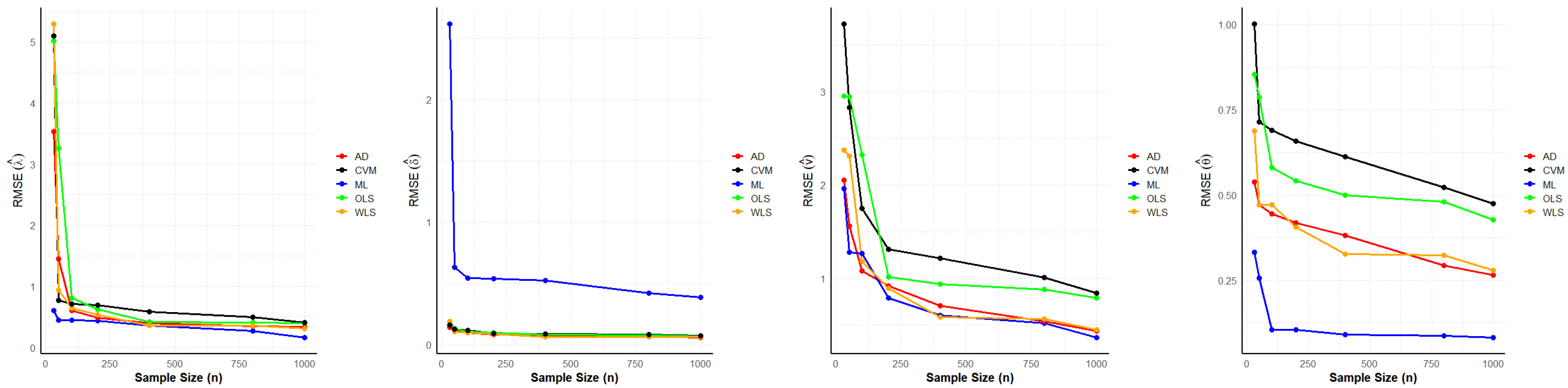
| Parameter | m | ML | AD | RMSE OLS | WLS | CVM | ML | AD | Abias OLS | WLS | CVM |
|---|---|---|---|---|---|---|---|---|---|---|---|
| 30 | 0.5988 (1) | 3.5330 (2) | 5.0166 (3) | 5.2952 (5) | 5.0907 (4) | −0.3870 (1) | 0.6461 (2) | 2.0737 (4) | 2.7005 (3) | 2.3113 (5) | |
| 30 | 2.6190 (5) | 0.1428 (1) | 0.1886 (3) | 0.1912 (4) | 0.1599 (2) | 0.7468 (5) | −0.0208 (2) | −0.0340 (3) | 0.0183 (1) | −0.0584 (4) | |
| v | 30 | 1.9582 (1) | 2.0534 (2) | 2.9499 (4) | 2.3728 (3) | 3.7246 (5) | 1.0438 (3) | 0.8529 (1) | 1.7460 (4) | 0.8609 (2) | 2.1656 (5) |
| 30 | 0.3320 (1) | 0.5388 (2) | 0.8533 (4) | 0.6874 (3) | 1.0024 (5) | 0.2114 (3) | 0.1538 (2) | 0.5694 (5) | 0.1261 (1) | 0.4884 (4) | |
| Sum of Ranks | 8 | 7 | 14 | 15 | 16 | 12 | 7 | 16 | 7 | 18 | |
| 50 | 0.4441 (1) | 1.4505 (4) | 3.2583 (5) | 0.9318 (3) | 0.7657 (2) | −0.3360 (2) | 0.3364 (3) | 0.8622 (5) | 0.3719 (4) | 0.0739 (1) | |
| 50 | 0.6299 (5) | 0.1167 (2) | 0.1320 (4) | 0.1044 (1) | 0.1263 (3) | 0.4163 (5) | −0.0111 (1) | −0.0297 (3) | −0.0118 (2) | −0.0584 (4) | |
| v | 50 | 1.2797 (1) | 1.5626 (2) | 2.9412 (5) | 2.3106 (3) | 2.8286 (4) | 1.0133 (3) | 0.5326 (2) | 1.7347 (5) | 0.4816 (1) | 1.2098 (4) |
| 50 | 0.2557 (1) | 0.4711 (3) | 0.7871 (5) | 0.4710 (2) | 0.7143 (4) | 0.1698 (3) | 0.0970 (2) | 0.4738 (5) | 0.0772 (1) | 0.3009 (4) | |
| Sum of Ranks | 8 | 11 | 19 | 9 | 13 | 13 | 8 | 18 | 8 | 13 | |
| 100 | 0.4436 (1) | 0.6051 (2) | 0.8122 (5) | 0.6433 (3) | 0.7131 (4) | −0.2004 (2) | 0.2430 (5) | 0.2143 (4) | 0.2098 (3) | 0.0396 (1) | |
| 100 | 0.5436 (5) | 0.0976 (2) | 0.1053 (3) | 0.0956 (1) | 0.1148 (4) | 0.4496 (5) | −0.0051 (1) | −0.0255 (3) | 0.0061 (2) | −0.0517 (4) | |
| v | 100 | 1.2634 (2) | 1.0762 (1) | 2.3179 (5) | 1.1842 (3) | 1.7482 (4) | 0.2501 (1) | 0.3681 (3) | 0.8583 (4) | 0.3523 (2) | 1.0001 (5) |
| 100 | 0.1054 (1) | 0.4452 (2) | 0.5813 (4) | 0.4706 (3) | 0.6890 (5) | 0.0616 (2) | 0.0173 (1) | 0.1784 (4) | 0.0644 (3) | 0.3028 (5) | |
| Sum of Ranks | 9 | 7 | 17 | 10 | 17 | 10 | 10 | 15 | 10 | 15 | |
| 200 | 0.4369 (1) | 0.4826 (2) | 0.6204 (4) | 0.5322 (3) | 0.6878 (5) | −0.1206 (2) | 0.1238 (3) | 0.2131 (5) | 0.1986 (4) | 0.0209 (1) | |
| 200 | 0.5385 (5) | 0.0829 (1) | 0.0965 (4) | 0.0885 (2) | 0.0915 (3) | 0.4821 (5) | −0.0044 (1) | 0.0151 (3) | 0.0056 (2) | −0.0460 (4) | |
| v | 200 | 0.7909 (1) | 0.9209 (3) | 1.0134 (4) | 0.8917 (2) | 1.3076 (5) | 0.1958 (1) | 0.2438 (3) | 0.3037 (4) | 0.2048 (2) | 0.6181 (5) |
| 200 | 0.1038 (1) | 0.4187 (3) | 0.5423 (4) | 0.4064 (2) | 0.6586 (5) | 0.0109 (1) | 0.0150 (2) | 0.1457 (4) | −0.0192 (3) | 0.2754 (5) | |
| Sum of Ranks | 8 | 9 | 16 | 9 | 18 | 9 | 9 | 16 | 11 | 15 | |
| 400 | 0.3558 (1) | 0.3975 (3) | 0.4130 (4) | 0.3583 (2) | 0.5865 (5) | −0.0546 (2) | 0.1233 (4) | 0.0974 (3) | 0.1708 (5) | 0.0207 (1) | |
| 400 | 0.5236 (5) | 0.0761 (2) | 0.0828 (3) | 0.0639 (1) | 0.0863 (4) | 0.5011 (5) | 0.0005 (1) | 0.0075 (3) | 0.0020 (2) | −0.0238 (4) | |
| v | 400 | 0.6038 (2) | 0.7090 (3) | 0.9378 (4) | 0.5844 (1) | 1.2151 (5) | −0.1191 (2) | 0.1252 (3) | 0.2169 (4) | 0.0915 (1) | 0.5436 (5) |
| 400 | 0.0901 (1) | 0.3813 (3) | 0.4996 (4) | 0.3269 (2) | 0.6118 (5) | 0.0073 (1) | 0.0173 (3) | 0.0751 (4) | 0.0165 (2) | 0.2644 (5) | |
| Sum of Ranks | 9 | 11 | 15 | 6 | 19 | 10 | 11 | 14 | 10 | 15 | |
| 800 | 0.2650 (1) | 0.3450 (2) | 0.4077 (4) | 0.3559 (3) | 0.4990 (5) | −0.0347 (2) | 0.0911 (4) | 0.0451 (3) | 0.1247 (5) | 0.0196 (1) | |
| 800 | 0.4192 (5) | 0.0658 (2) | 0.0751 (3) | 0.0638 (1) | 0.0794 (4) | 0.4172 (5) | −0.0004 (1) | −0.0140 (4) | 0.0014 (2) | −0.0115 (3) | |
| v | 800 | 0.5210 (1) | 0.5417 (2) | 0.8795 (4) | 0.5677 (3) | 1.0105 (5) | 0.1056 (3) | 0.0795 (1) | 0.2434 (4) | 0.0512 (2) | 0.3884 (5) |
| 800 | 0.0875 (1) | 0.2932 (2) | 0.4798 (4) | 0.3239 (3) | 0.5229 (5) | 0.0057 (1) | 0.0134 (4) | 0.0131 (3) | −0.0112 (2) | 0.1593 (5) | |
| Sum of Ranks | 8 | 8 | 15 | 10 | 19 | 11 | 10 | 14 | 11 | 14 | |
| 1000 | 0.1556 (1) | 0.3409 (3) | 0.3957 (4) | 0.3121 (2) | 0.4092 (5) | −0.0356 (2) | 0.0396 (3) | 0.0435 (4) | 0.1186 (5) | 0.0164 (1) | |
| 1000 | 0.3862 (5) | 0.0551 (1) | 0.0666 (3) | 0.0613 (2) | 0.0696 (4) | 0.4862 (5) | −0.0003 (1) | −0.0053 (3) | 0.0013 (2) | −0.0067 (4) | |
| v | 1000 | 0.3626 (1) | 0.4385 (2) | 0.7884 (4) | 0.4497 (3) | 0.8383 (5) | −0.4626 (5) | 0.0413 (2) | 0.2010 (3) | −0.0198 (1) | 0.2736 (4) |
| 1000 | 0.0809 (1) | 0.2651 (2) | 0.4276 (4) | 0.2790 (3) | 0.4752 (5) | 0.0039 (1) | −0.0132 (4) | 0.0130 (3) | −0.0118 (2) | 0.1448 (5) | |
| Sum of Ranks | 8 | 8 | 15 | 10 | 19 | 13 | 10 | 13 | 10 | 14 |
| Parameters | m | ML | AD | OLS | WLS | CVM |
|---|---|---|---|---|---|---|
| 30 | 25 (3) | 23 (2) | 27 (4) | 16 (1) | 29 (5) | |
| 50 | 24 (2) | 27 (3.5) | 28 (5) | 14 (1) | 27 (3.5) | |
| 100 | 20 (2) | 30 (5) | 23 (3) | 19 (1) | 28 (4) | |
| 200 | 19 (1) | 34 (5) | 21 (3) | 20 (2) | 26 (4) | |
| 400 | 18 (1) | 32 (5) | 22 (3) | 21 (2) | 27 (4) | |
| 800 | 17 (1) | 29 (5) | 25 (3) | 22 (2) | 27 (4) | |
| 1000 | 10 (1) | 32 (5) | 26 (3) | 24 (2) | 28 (4) | |
| 30 | 20 (2) | 14 (1) | 30 (4) | 22 (3) | 34 (5) | |
| 50 | 21 (3) | 19 (1) | 37 (5) | 17 (2) | 26 (4) | |
| 100 | 19 (2) | 17 (1) | 32 (4.5) | 20 (3) | 32 (4.5) | |
| 200 | 17 (1) | 18 (2) | 32 (4) | 20 (3) | 33 (5) | |
| 400 | 19 (2) | 22 (3) | 29 (4) | 16 (1) | 34 (5) | |
| 800 | 19 (2) | 18 (1) | 29 (4) | 21 (3) | 33 (5) | |
| 1000 | 21 (3) | 18 (1) | 28 (4) | 20 (2) | 33 (5) | |
| Sum of Ranks | 26 | 40.5 | 53.5 | 28 | 62 | |
| Overall rank | 1 | 3 | 4 | 2 | 5 |
| Estimates | GoF Statistics | |||||||||||
|---|---|---|---|---|---|---|---|---|---|---|---|---|
| Model | −2log(L) | AIC | CAIC | BIC | K-S | p-Value | ||||||
| ExpH-W | 1.7840 | 3.1373 | 15.3200 | 0.6743 | 153.0958 | 161.0958 | 162.4291 | 167.3172 | 0.0305 | 0.1986 | 0.0867 | 0.9549 |
| (0.7689) | (2.8483 ) | (1.4245) | (0.06487) | |||||||||
| v | ||||||||||||
| HW | ||||||||||||
| a | b | |||||||||||
| RBTIIEHLTLW | 1.9022 | 4.9008 | 134.3900 | 0.06787 | 163.6136 | 171.6136 | 172.947 | 177.8350 | 0.1477 | 0.933 | 0.1463 | 0.4424 |
| (0.37494) | (3.9165 ) | (0.02882) | (4.9684 ) | |||||||||
| a | b | |||||||||||
| WLx | 2.2065 | 4.4219 | 7.7393 | 0.8239 | 161.0881 | 169.0881 | 170.4215 | 175.3095 | 0.1103 | 0.7102 | 0.1232 | 0.6631 |
| (5.0757 ) | (1.8868) | (1.3194 ) | (1.3124) | |||||||||
| OLLEW | 0.0115 | 0.0908 | 3.5189 | 14.6611 | 158.6735 | 166.6735 | 168.0068 | 172.8949 | 0.0573 | 0.4133 | 0.0990 | 0.8829 |
| (0.0193) | (0.0124) | (0.7393) | (0.0966) | |||||||||
| EHLWP | 7.0598 | 5.0729 | 8.0153 | 1.7194 | 160.3848 | 168.3848 | 169.7182 | 174.6062 | 0.1026 | 0.663 | 0.12098 | 0.6849 |
| (8.4735 ) | (8.3097 ) | (1.0306 ) | (3.3213 ) | |||||||||
| ELOLLW | 2.6629 | 6.4083 | 6.6610 | 1.9932 | 164.9772 | 172.9772 | 174.3105 | 179.1986 | 0.1639 | 1.0262 | 0.1454 | 0.4500 |
| (2.1143) | (1.2802 ) | (1.8971 ) | (0.2437) | |||||||||
| v | ||||||||||||
| HWP | 1.3697 | 7.9607 | 0.6445 | 6.0891 | 155.5646 | 163.5646 | 164.8979 | 169.786 | 0.0382 | 0.2585 | 0.1098 | 0.7930 |
| (5.7727 ) | (4.5399 ) | (5.5434 ) | (0.5655) | |||||||||
| a | b | |||||||||||
| KumW | 48.7672 | 34.5299 | 16.7869 | 0.2135 | 160.2115 | 168.2115 | 169.5449 | 174.4329 | 0.1002 | 0.6496 | 0.1213 | 0.6819 |
| (4.4684) | (0.6746) | (4.2412) | (0.0183) |
| Estimates | GoF Statistics | |||||||||||
|---|---|---|---|---|---|---|---|---|---|---|---|---|
| Model | −2log(L) | AIC | CAIC | BIC | K-S | p-Value | ||||||
| ExpH-W | 0.9471 | 4.8750 | 13.0410 | 0.4956 | 197.8110 | 205.8110 | 206.7866 | 213.1256 | 0.0270 | 0.1883 | 0.0639 | 0.9918 |
| (0.2949) | (6.2641 ) | (2.7982) | (5.3574 ) | |||||||||
| v | ||||||||||||
| HW | ||||||||||||
| a | b | |||||||||||
| RBTIIEHLTLW | 5.0497 | 4.9008 | 1.3699 | 4.2824 | 204.9325 | 212.9325 | 213.9081 | 220.247 | 0.0928 | 0.6568 | 0.1167 | 0.5585 |
| (0.3531) | (6.2536 ) | (4.4681 ) | (3.4922 ) | |||||||||
| a | b | |||||||||||
| WLx | 4.7329 | 2.4865 | 3.0636 | 0.2239 | 200.6681 | 208.6681 | 209.6437 | 215.9826 | 0.0569 | 0.3680 | 0.0949 | 0.8015 |
| (2.3553 ) | (1.4675) | (1.8319 ) | (0.5191) | |||||||||
| OLLEW | 0.0012 | 0.0462 | 2.4555 | 14.8432 | 202.4335 | 210.4335 | 211.4091 | 217.7481 | 0.0758 | 0.4579 | 0.0941 | 0.8105 |
| (0.0093) | (0.0110) | (1.0908) | (0.0654) | |||||||||
| EHLWP | 6.3669 | 6.1644 | 8.0412 | 9.5572 | 200.5537 | 208.5537 | 209.5293 | 215.8683 | 0.0573 | 0.3482 | 0.0923 | 0.8276 |
| (1.6357 ) | (0.2137) | (1.5626 ) | (6.3483) | |||||||||
| ELOLLW | 1.2322 | 3.5026 | 6.7826 | 0.8985 | 208.9394 | 216.9394 | 217.915 | 224.254 | 0.1298 | 0.9009 | 0.1204 | 0.5170 |
| (1.5449) | (1.2110 ) | (6.9530 ) | (9.5760 ) | |||||||||
| v | ||||||||||||
| HWP | 4.8635 | 1.3634 | 0.5314 | 8.9756 | 200.4499 | 208.4499 | 209.4255 | 215.7645 | 0.034 | 0.2407 | 0.1138 | 0.5912 |
| (2.3895 ) | (90.5960) | (5.0737 ) | (2.1548) | |||||||||
| a | b | |||||||||||
| KumW | ||||||||||||
Disclaimer/Publisher’s Note: The statements, opinions and data contained in all publications are solely those of the individual author(s) and contributor(s) and not of MDPI and/or the editor(s). MDPI and/or the editor(s) disclaim responsibility for any injury to people or property resulting from any ideas, methods, instructions or products referred to in the content. |
© 2026 by the authors. Licensee MDPI, Basel, Switzerland. This article is an open access article distributed under the terms and conditions of the Creative Commons Attribution (CC BY) license.
Share and Cite
Charumbira, W.F.; Almongy, H.M.; Chipepa, F.; Pararai, M. Exploring the New Exponentiated Harris-G Family of Distributions and Its Applications. Symmetry 2026, 18, 673. https://doi.org/10.3390/sym18040673
Charumbira WF, Almongy HM, Chipepa F, Pararai M. Exploring the New Exponentiated Harris-G Family of Distributions and Its Applications. Symmetry. 2026; 18(4):673. https://doi.org/10.3390/sym18040673
Chicago/Turabian StyleCharumbira, Wellington F., Hisham M. Almongy, Fastel Chipepa, and Mavis Pararai. 2026. "Exploring the New Exponentiated Harris-G Family of Distributions and Its Applications" Symmetry 18, no. 4: 673. https://doi.org/10.3390/sym18040673
APA StyleCharumbira, W. F., Almongy, H. M., Chipepa, F., & Pararai, M. (2026). Exploring the New Exponentiated Harris-G Family of Distributions and Its Applications. Symmetry, 18(4), 673. https://doi.org/10.3390/sym18040673