A Novel Extension of the Weibull Distribution with Application in Quantitative and Reliability Sciences


Abstract
1. Introduction
2. A New Flexible Exponentiated Generalization of the Weibull Distribution
2.1. Linear Expansion of the PDF of the SEW Distribution
2.2. Moments of SEW Distribution
Standard Deviation, Skewness, and Kurtosis: Analytical Interpretation
2.3. Reliability Analysis
2.4. Quantile Function (QF) of SEW Distribution
2.5. Lorenz and Bonferroni Curves of SEW Distribution
2.6. Absolute Deviations from the Mean and Median of the SEW Distribution
2.7. Mean Waiting Time and Mean Residual Life of the SEW Distribution
2.8. Renyi Entropy and Tsallis Entropy of the SEW Distribution
3. Parameter Estimation of SEW Distribution via SRS and RSS
3.1. ML Estimator of SEW Distribution via SRS
3.2. ML Estimators of SEW Distribution via RSS
- 1.
- First, draw items at random from the population, followed by random allocation into m subsets, with each subset containing m units.
- 2.
- Use a simple and inexpensive method to rank the units within each set.
- 3.
- From each ith set, for , select the unit that ranks ith.
- 4.
- Repeat the above steps j times to obtain a final sample of size .
3.3. Simulation Procedures: SRS and RSS
- The simulation procedure follows the steps below.
- 1.
- For each sampling scheme (SRS and RSS), generate a sample of size using the proposed distribution with selected parameter combinations. In the case of RSS, appropriate set size m and number of cycles j are chosen such that .
- 2.
- The following parameter settings are used in the simulations:
- 3.
- For each combination, we compute the ML estimators of the parameters under both the SRS and RSS schemes.
- 4.
- Repeat steps 1–3 for iterations. For each case, calculate the MSE of the estimated parameters over the repetitions.
- 5.
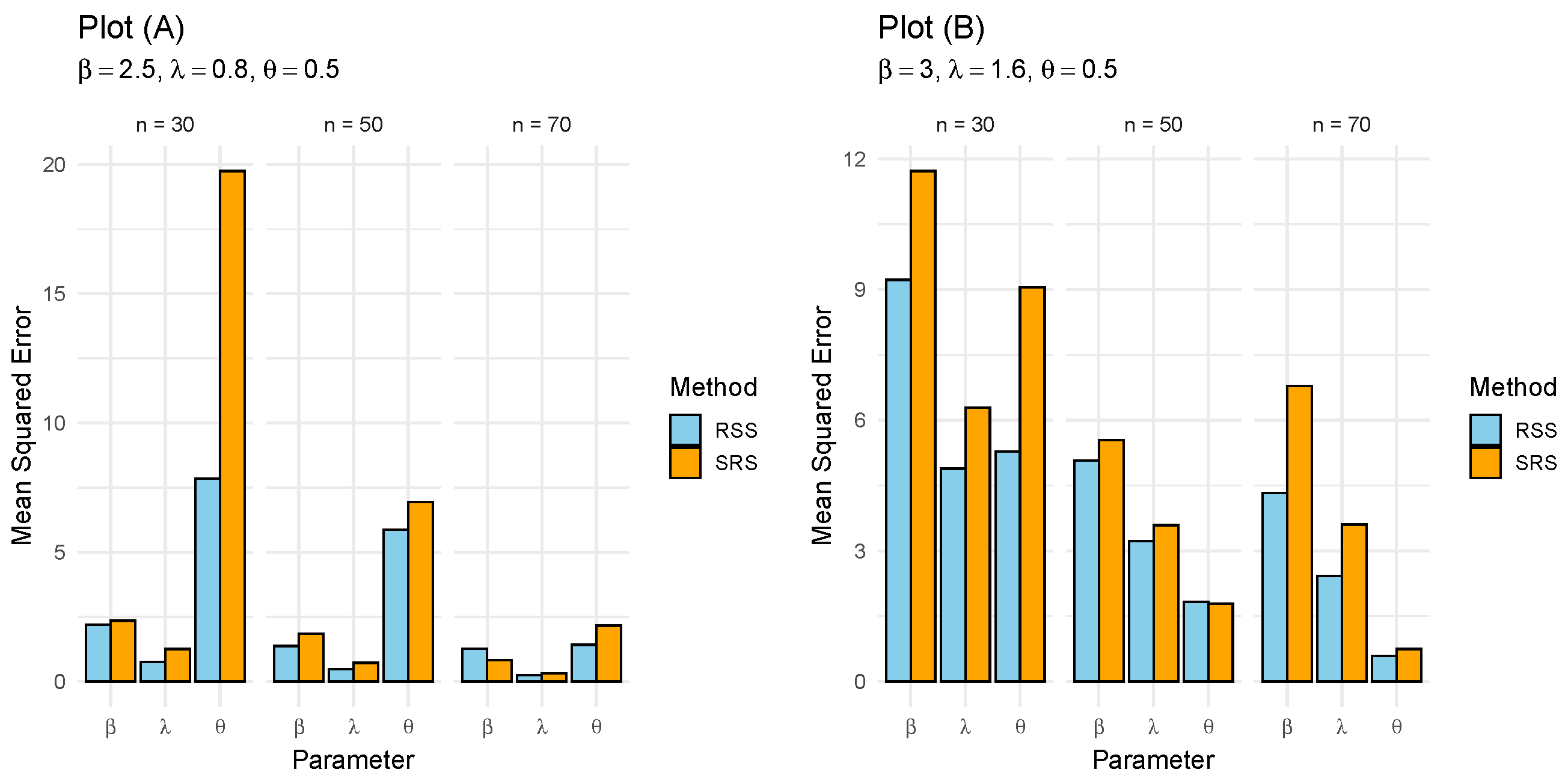
- The computed MSE values for different scenarios are summarized graphically in Figure 3 below.
4. Estimation of Parameters Through Different Methods of Estimation
Simulation Study
- Different sample sizes, such as , and different parametric values, such as , are considered for the simulation process. For each case, Monte Carlo replications are conducted through the quantile function of the SEW distribution in the R (version 4.1.2). The main aim of this simulation is to check the accuracy and efficiency of the different estimators for different sample sizes and to find the best estimation method for the SEW model under SRS. Superscripts denote ranking of estimators based on performance (1 = best, higher numbers indicate lower performance). The simulation results are arranged in Table 3, Table 4, Table 5 and Table 6 given below.
- The simulation outcomes in Table 3, Table 4, Table 5 and Table 6 demonstrate the performance of the different estimation procedures in terms of the AB, MSE, and MRE for sample sizes and 300. The ranks of each procedure, summed to provide a combined measure of performance, were obtained based on the AB, MSE, and MRE. The outcomes of the simulation reveal that the accuracy of estimation increases with an increase in sample size, validating the consistency of the estimators and also highlighting the differences in the efficiency and stability of the estimators. Table 7 presents a summary of the overall ranking of the estimation procedures for all parameter combinations and sample sizes. MPSE appears to be the most promising estimator, followed by WLSE and MLE, which show better accuracy in their estimation results. The MPSE, MLE, and ADE methods show moderate performance, whereas OLSE, WLSE, and CVME show poor performance in estimation due to higher bias and variability in the results. shows superior results, providing the most reliable estimations.
5. Distribution of Order Statistics from SEW Distribution
5.1. Univariate Case
Moment of Order Statistics
5.2. Reversed Order Statistics
Moment of Reversed Order Statistics
5.3. Upper Record Statistics of SEW Distribution
Moment of Upper Record Statistics
6. Applications
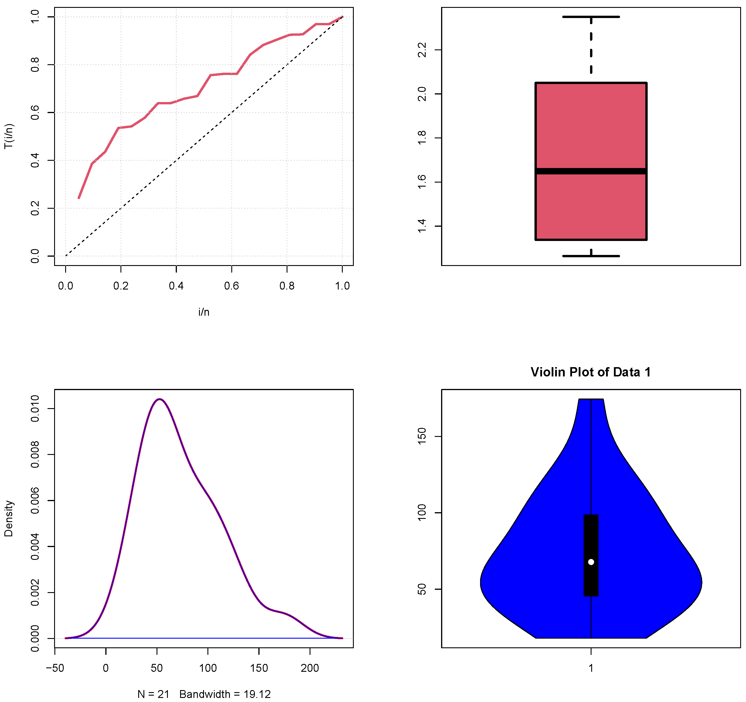
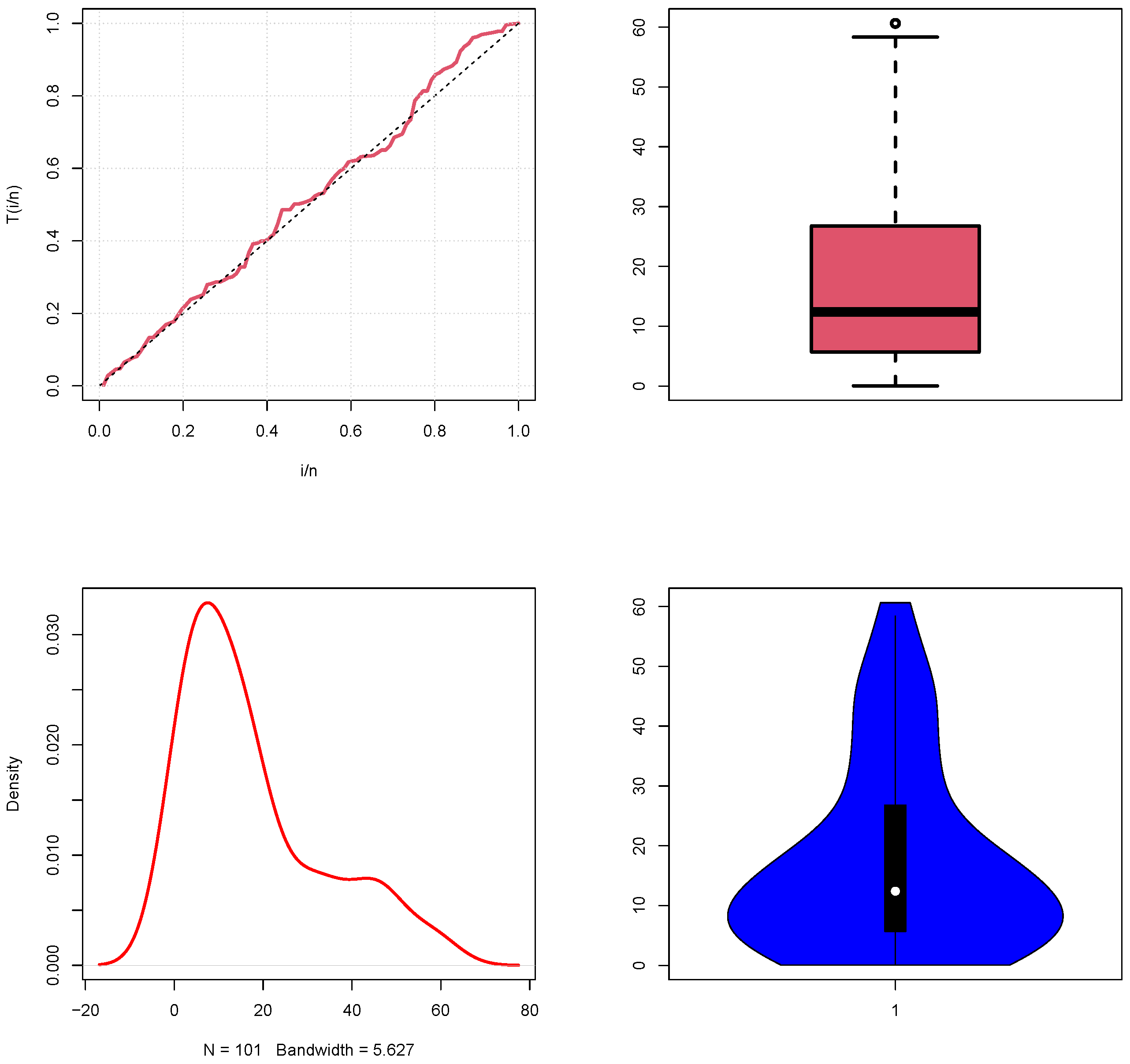
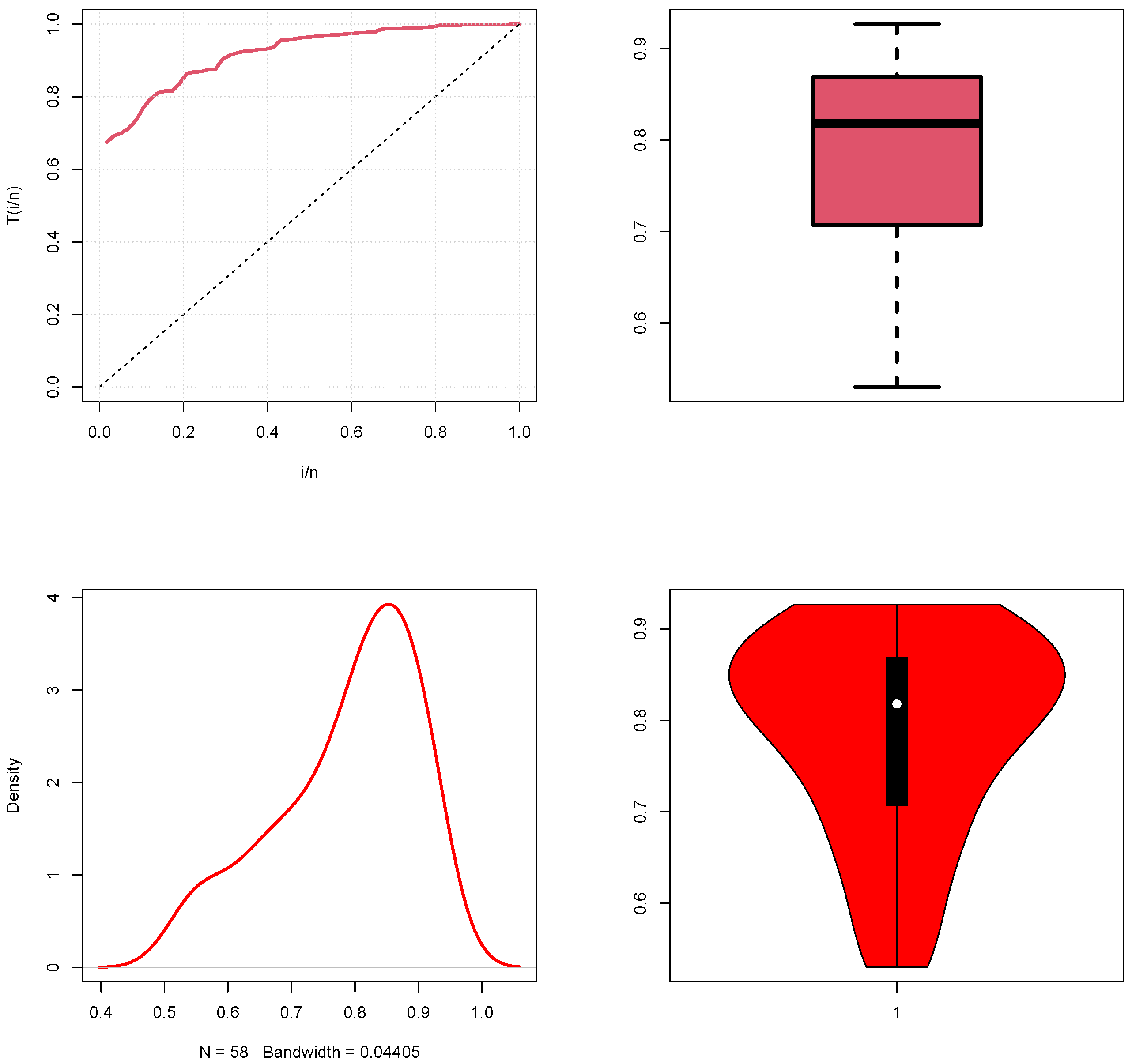
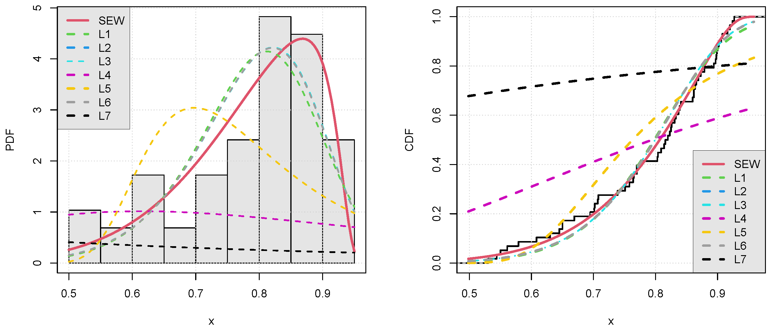
- The first dataset represents the number of millions of revolutions completed by each of 23 ball bearings before experiencing failure during an endurance test [53]. The recorded values are presented as follows. Data I: 17.88, 28.92, 33.00, 41.52, 42.12, 45.60, 51.84, 51.96, 54.12, 55.56, 67.80 68.64, 68.64, 84.12, 93.12, 98.64, 105.12, 105.84, 127.92, 128.04, 174.40.Data 2: The second dataset represents 101 cases of progressed acute myelogenous leukemia registered at the International Bone Marrow Transplant Registry (see [54]). The data are as follows. Data II: 0.030, 0.493,0.855, 1.184, 1.283, 1.480, 1.776, 2.138, 2.500, 2.763, 2.993, 3.224, 3.421, 4.178, 4.441, 5.691, 5.855, 6.941, 6.941, 7.993, 8.882, 8.882, 9.145, 11.480, 11.513, 12.105, 12.796, 12.993, 13.849, 16.612, 17.138, 20.066, 20.329, 22.368, 26.776, 28.717, 28.717, 32.928, 33.783, 34.211, 34.770, 39.539, 41.118, 45.033, 46.053, 46.941, 48.289, 57.401, 58.322, 60.625, 0.658, 0.822, 1.414, 2.500, 3.322, 3.816, 4.737, 4.836, 4.934, 5.033, 5.757, 5.855, 5.987, 6.151, 6.217, 6.447, 8.651, 8.717, 9.441, 10.329, 11.480, 12.007, 12.007, 12.237, 12.401, 13.059, 14.474, 15.000, 15.461, 15.757, 16.480, 16.711, 17.204, 17.237, 17.303, 17.664, 18.092, 18.092, 18.750, 20.625, 23.158, 27.730, 31.184, 32.434, 35.921, 42.237, 44.638, 46.480, 47.467, 48.322, 56.086.The third dataset corresponds to unemployment claim data (see [55]). This dataset consists of 58 bounded observations representing unemployment claim rates in proportion form. The observed data are as follows. Data III: 0.823, 0.864, 0.816, 0.841, 0.831, 0.833, 0.894, 0.869, 0.866, 0.860, 0.837, 0.826, 0.804, 0.809, 0.758, 0.770, 0.778, 0.707, 0.814, 0.825, 0.906, 0.924, 0.927, 0.920, 0.770, 0.544, 0.550, 0.608, 0.630, 0.650, 0.820, 0.873, 0.900, 0.916, 0.899, 0.862, 0.695, 0.650, 0.751, 0.862, 0.702, 0.530, 0.764, 0.898, 0.897, 0.908, 0.902, 0.879, 0.645, 0.739, 0.765, 0.803, 0.708, 0.669, 0.561, 0.579, 0.701, 0.839.In this study, the proposed SEW model is compared with well-known and competitive lifetime models to assess its flexibility and potential for modeling real-life data. For comparison purposes, we use a new modification of the Weibull distribution (L1) by [4], the additive Weibull model (L2) by [56], the Beta-Weibull model (L3) by [6], a new technique of adding a parameter to the Weibull distribution (L4) by [57], the inverse Weibull distribution (L5) by [58], the Burr family of cumulative frequency functions (L6) by [59], and the log-transformed generalized family of distributions (L7) by [60]. The comparison is carried out on the basis of well-established goodness-of-fit criteria such as the Akaike information criterion (), Bayesian information criterion (), corrected Akaike information criterion (), and Hannan–Quinn information criterion (). Additionally, the traditional measures of the Cramér–von Mises statistic W, Anderson–Darling statistic A, Kolmogorov–Smirnov statistic , and p-value are used. For the descriptive analysis of the datasets, graphical tools such as the plot, boxplot, kernel density, and violin plot are also employed.
- The graphs plotted for the three datasets are shown in Figure 4, Figure 5 and Figure 6. According to Figure 4, the first dataset yields a graph with an increasing trend, which implies that there is an increasing hazard rate. The boxplot and density plot provide additional information about minimal deviations on the right side, which implies stability. On the other hand, the second dataset, as presented in Figure 5, has an approximately linear shape in the TTT plot, which means that the dataset has a constant hazard rate. However, it is evident that there is wide dispersion, with the possibility of outliers, and that there is a right-skewed distribution in the density plot. From Figure 6, the third dataset has an increasing TTT plot, implying an increasing hazard rate, while the boxplot and kernel density have left-skewed.
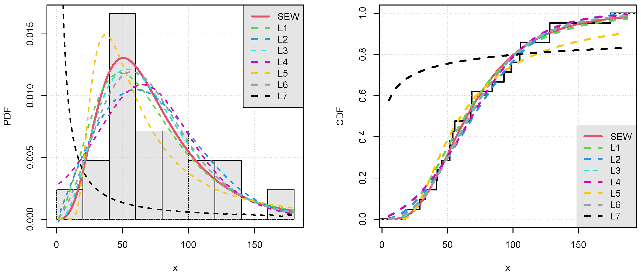
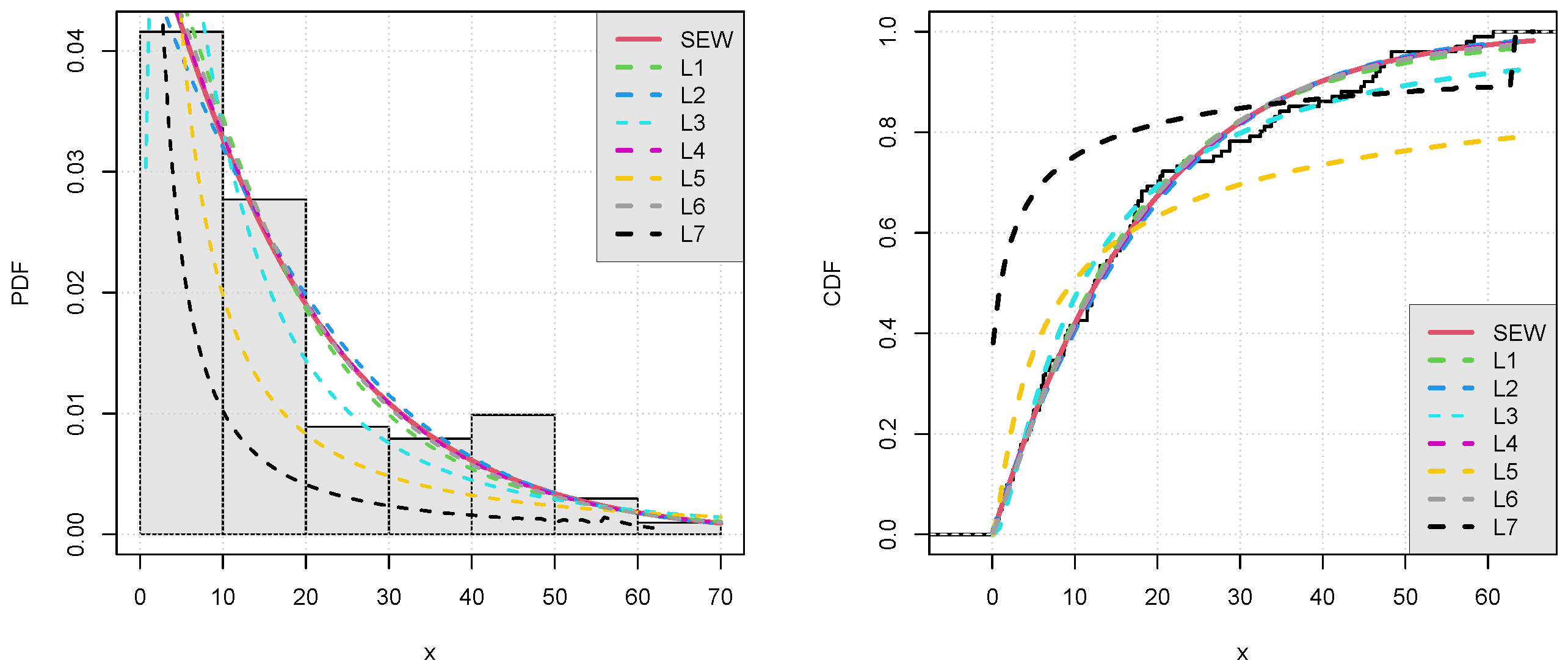
- The practical applicability and efficacy of the proposed SEW model are demonstrated by employing the model on real-life datasets, and the results are presented in terms of the goodness-of-fit statistics, as given in Table 8, Table 9 and Table 10 and likelihood estimates and standard errors, as given in Table 11, Table 12 and Table 13. Whereas the fit of the proposed SEW model is further demonstrated by Figure 7, Figure 8 and Figure 9. It can be seen from Table 8 that the SEW model significantly outperforms the other models in terms of the log-likelihood and information criteria, including the AIC, CAIC, BIC, and HQIC, on Dataset 1. In addition, L1–L6 display comparatively poorer performance than the SEW model in fitting Dataset 1, and L7 shows an extremely poor fit as revealed by large KS values and an almost zero p-value, as evidenced in Figure 7. On Dataset 2, the SEW model exhibits strong fitting and reliability, while L4 and L6 show relative superiority in comparison with the other models, but they are still somewhat inferior to the SEW model, and L3, L5, and L7 provide a poor fit because of their large KS statistics and small p-values, as shown in Figure 8. Finally, for Dataset 3, it can be seen from Table 10 that the SEW model displays an excellent fit in terms of the maximum log-likelihood and minimal information criteria, whereas L1–L3 and L6 demonstrate moderate fitting and L4 and L7 show poor fitting for Dataset 3, as evident from Figure 9. Moreover, Table 11, Table 12 and Table 13 shows that the standard errors are relatively small, which confirms the reliability and stability of the proposed model. Therefore, based on three Dataset, the SEW model demonstrates better performance and greater estimation efficiency compared to the competing models.
- From the above analysis, we can conclude that the proposed SEW model is better than the compared models based on statistical measures such as the log-likelihood, information criteria, and goodness of fit. Most of the existing models are either incapable of capturing the underlying distribution or offer poor goodness of fit, especially when considering the p-values and KS statistics, while the proposed model shows stability and flexibility across all datasets under study. Finally, from the above, it can be concluded that the proposed SEW model is highly efficient and effective, as it offers better statistical performance and superior goodness of fit compared to all other available models.
7. Actuarial Measures
7.1. Value at Risk
7.2. Expected Shortfall
7.3. Tail Value at Risk
7.4. Tail Variance
7.5. Tail Variance Premium
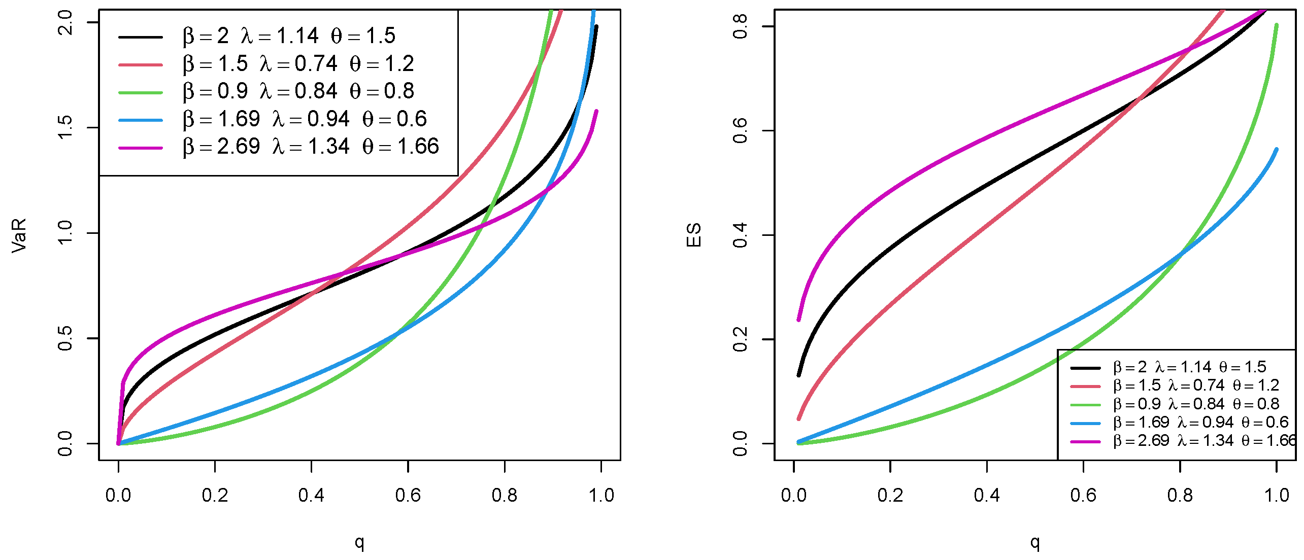
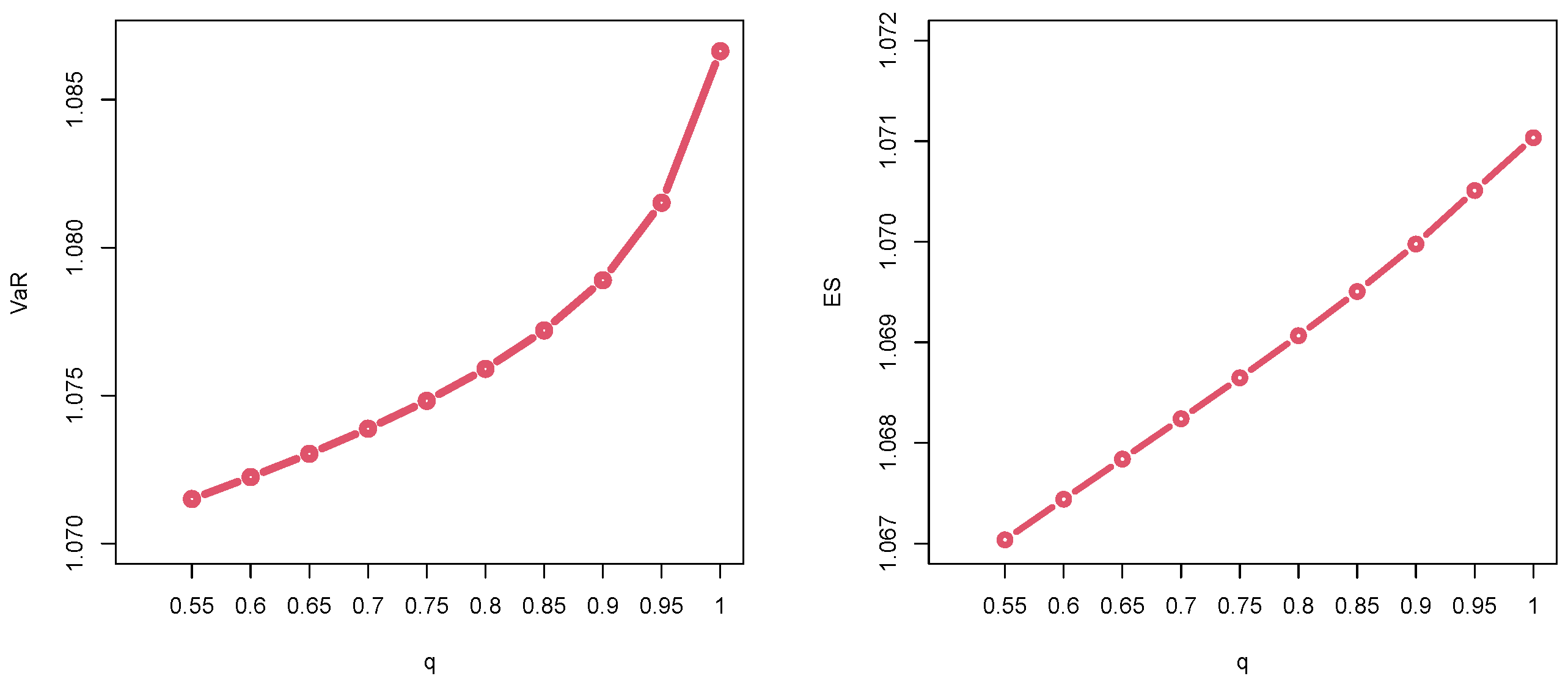
Numerical Illustration of VaR and ES
8. Conclusions
Author Contributions
Funding
Data Availability Statement
Conflicts of Interest
References
- Meeker, W.Q.; Escobar, L.A.; Pascual, F.G. Statistical Methods for Reliability Data; John Wiley and Sons: Hoboken, NJ, USA, 2021. [Google Scholar]
- Gaidai, O.; Yakimov, V.; Wang, F.; Cao, Y. Gaidai multivariate reliability method for energy harvester operational safety, given manufacturing imperfections. Int. J. Precis. Eng. Manuf. 2024, 25, 1011–1025. [Google Scholar] [CrossRef]
- Embrechts, P.; Kluppelberg, C.; Mikosch, T. Modelling Extremal Events: For Insurance and Finance; Springer Science and Business Media: Berlin/Heidelberg, Germany, 2013; Volume 33. [Google Scholar]
- Alshanbari, H.M.; Ahmad, Z.; El-Bagoury, A.A.A.H.; Odhah, O.H.; Rao, G.S. A new modification of the Weibull distribution: Model, theory, and analyzing engineering data sets. Symmetry 2024, 16, 611. [Google Scholar] [CrossRef]
- Mudholkar, G.S.; Srivastava, D.K. Exponentiated Weibull family for analyzing bathtub failure-rate data. IEEE Trans. Reliab. 1993, 42, 299–302. [Google Scholar] [CrossRef]
- Famoye, F.; Lee, C.; Olumolade, O. The beta-Weibull distribution. J. Stat. Theory Appl. 2005, 4, 121–136. [Google Scholar]
- Keller, A.Z.; Kamath, A.R.R.; Perera, U.D. Reliability analysis of CNC machine tools. Reliab. Eng. 1982, 3, 449–473. [Google Scholar] [CrossRef]
- Lai, C.D.; Xie, M.; Murthy, D.N.P. A modified Weibull distribution. IEEE Trans. Reliab. 2003, 52, 33–37. [Google Scholar] [CrossRef]
- Shama, M.S.; Alharthi, A.S.; Almulhim, F.A.; Gemeay, A.M.; Meraou, M.A.; Mustafa, M.S.; Aljohani, H.M. Modified generalized Weibull distribution: Theory and applications. Sci. Rep. 2023, 13, 12828. [Google Scholar] [CrossRef] [PubMed]
- Alsulami, D.; Alghamdi, A.S. A New Extended Weibull Distribution: Estimation Methods and Applications in Engineering, Physics, and Medicine. Mathematics 2025, 13, 3262. [Google Scholar] [CrossRef]
- Al-Moisheer, A.S.; Sultan, K.S.; Radwan, H.M. A novel adaptable Weibull distribution and its applications. Axioms 2025, 14, 490. [Google Scholar] [CrossRef]
- Zanboori, A.; Zanboori, E.; Parvin, H.; Mahmoudi, M. A flexible Weibull geometric distribution with characterizations and its parameter estimation. Sci. Rep. 2025, 15, 26372. [Google Scholar] [CrossRef]
- Li, X.; Gong, Q.; Chen, T. Statistical inference and applications of a new transforming Weibull distribution. Sci. Rep. 2025, 15, 28970. [Google Scholar] [CrossRef]
- Begum, S.; Karim, M.R. The modified kies-weibull distribution: A flexible model for survival analysis. Int. J. Data Sci. Anal. 2025, 11, 6–16. [Google Scholar] [CrossRef]
- Chaturvedi, P.; Pokhriyal, H. Parameter estimation of the four-parameter Harris extended Weibull distribution with applications to real-life data. arXiv 2025, arXiv:2509.26162. [Google Scholar]
- Ahmed, Z.A.; Mohammed, A.T.; Enver, A. New Lifetime Alpha Power Rayleigh Weibull Distribution: Structure and Properties. Ibn AL-Haitham J. Pure Appl. Sci. 2025, 38, 352–362. [Google Scholar] [CrossRef]
- Gbemiga, A.S.; Afolabi, J.M. Development of Gompertz Generalised Weibull Distribution: Properties and Applications. Frontline Prof. J. 2025, 2, 24–34. [Google Scholar]
- Abdelkawy, M.A.; Alghamdi, S.M.; Elbatal, I.; Hashem, A.F.; Shawki, A.W.; Elgarhy, M. Statistical analysis of disability: Utilizing the new extended Rayleigh inverted Weibull model. Alex. Eng. J. 2025, 129, 779–792. [Google Scholar] [CrossRef]
- El-Saeed, A.R.; Elbatal, I.; Almetwally, E.M.; Elgarhy, M. Bayesian and Non-Bayesian Inference for the Trigonometric Extended Rayleigh-Weibull Model Under Progressively Censored Data. IEEE Access 2025, 13, 117043–117064. [Google Scholar] [CrossRef]
- Elgarhy, M.; Abdalla, G.S.S.; Obulezi, O.J.; Almetwally, E.M. A tangent DUS family of distributions with applications to the Weibull model. Sci. Afr. 2025, 29, e02843. [Google Scholar] [CrossRef]
- Bashiru, S.O.; Abdalla, G.S.S.; Ragab, I.E.; Elbatal, I.; Gemeay, A.M.; Elgarhy, M. Type II Half-Logistic Rayleigh Weibull distribution with statistical inference and applications. Sci. Afr. 2025, 30, e02927. [Google Scholar] [CrossRef]
- Nadir, S.; Ali, E.I.; Semary, H.E.; Aslam, M.; Obulezi, O.J.; Nasiru, S.; Elgarhy, M. Burr III Scaled Inverse Odds Ratio-Weibull Distribution for Modeling Asymmetric Medical and Engineering Data. Eng. Rep. 2025, 7, e70482. [Google Scholar] [CrossRef]
- Ado Osi, A.; Metwally, D.S.; Semary, H.E.; Ahmad Sabo, S.; Zakariyya Musa, I.; Hussein Mohamud, M.; Elgarhy, M. The New Heavy-Tailed Cosine-Weibull Distribution: Properties, Simulation, Applications, and Regression Modeling. Eng. Rep. 2025, 7, e70477. [Google Scholar] [CrossRef]
- Alotaibi, N.; Elbatal, I.; Almetwally, E.M.; Alyami, S.A.; Al-Moisheer, A.S.; Elgarhy, M. Bivariate Step-Stress Accelerated Life Tests for the Kavya-Manoharan Exponentiated Weibull Model under Progressive Censoring with Applications. Symmetry 2022, 14, 1791. [Google Scholar] [CrossRef]
- Alotaibi, N.; Elbatal, I.; Almetwally, E.M.; Alyami, S.A.; Al-Moisheer, A.S.; Elgarhy, M. Truncated Cauchy Power Weibull-G Class of Distributions: Bayesian and Non-Bayesian Inference Modelling for COVID-19 and Carbon Fiber Data. Mathematics 2022, 10, 1565. [Google Scholar] [CrossRef]
- Alyami, S.A.; Elbatal, I.; Alotaibi, N.; Almetwally, E.M.; Okasha, H.M.; Elgarhy, M. Topp-Leone Modified Weibull Model: Theory and Applications to Medical and Engineering Data. Appl. Sci. 2022, 12, 10431. [Google Scholar] [CrossRef]
- Almarashi, A.M.; Jamal, F.; Chesneau, C.; Elgarhy, M. The Exponentiated Truncated Inverse Weibull-Generated Family of Distributions with Applications. Symmetry 2020, 12, 650. [Google Scholar] [CrossRef]
- Aldahlan, M.A.; Jamal, F.; Chesneau, C.; Elbatal, I.; Elgarhy, M. Exponentiated power generalized Weibull power series family of distributions: Properties, estimation and applications. PLoS ONE 2020, 20, e0230004. [Google Scholar] [CrossRef]
- Alkarni, S.H.; Afify, A.Z.; Elbatal, I.; Elgarhy, M. The extended inverse Weibull distribution: Properties and applications. Complexity 2020, 2020, 3297693. [Google Scholar] [CrossRef]
- Hassan, A.S.; Elgarhy, M. Exponentiated Weibull-Weibull Distribution: Statistical Properties and Applications. Gazi J. Sci. 2019, 32, 616–635. [Google Scholar]
- Awadalla, M.; Murugesan, M. Bayesian Fractional Weibull Regression for Reliability Prognostics and Predictive Maintenance. Mathematics 2026, 14, 169. [Google Scholar] [CrossRef]
- Bourguignon, M.; Silva, R.B.; Cordeiro, G.M. The Weibull-G family of probability distributions. J. Data Sci. 2014, 12, 53–68. [Google Scholar] [CrossRef]
- Alzaatreh, A.; Famoye, F.; Lee, C. A new method for generating families of continuous distributions. Metron 2013, 71, 63–79. [Google Scholar] [CrossRef]
- Tahir, M.H.; Cordeiro, G.M.; Alizadeh, M.; Mansoor, M.; Zubair, M.; Hamedani, G.G. The odd generalized exponential family of distributions with applications. J. Stat. Distrib. Appl. 2015, 2, 1. [Google Scholar] [CrossRef]
- Kakwani, N.C.; Podder, N. Efficient estimation of the Lorenz curve and associated inequality measures from grouped observations. In Modeling Income Distributions and Lorenz Curves; Springer: New York, NY, USA, 2008; pp. 57–70. [Google Scholar]
- Elgarhy, M. Garhy distribution with different estimation methods and applications to engineering and medical data. Rev. Int. Métodos Numéricos Para Cálculo Diseño Ing. 2026, 1, 61. [Google Scholar]
- Pham-Gia, T.; Hung, T. The mean and median absolute deviations. Math. Comput. Model. 2001, 34, 921–936. [Google Scholar] [CrossRef]
- Al-Saleh, M.F.; Al-Hadhrami, S.A. Estimation of the mean of the exponential distribution using moving extremes ranked set sampling. Stat. Pap. 2003, 44, 367–382. [Google Scholar] [CrossRef]
- Chen, Z.; Bai, Z.; Sinha, B.K. Ranked Set Sampling: Theory and Applications; Springer: Berlin/Heidelberg, Germany, 2004; Volume 176. [Google Scholar]
- Imran, M.; Al-Essa, L.A.; Tahir, M.H.; Chesneau, C.; Shakoor, S.; Jamal, F. An extended exponential model: Estimation using ranked set sampling with applications. J. Radiat. Res. Appl. Sci. 2023, 16, 100642. [Google Scholar] [CrossRef]
- Bantan, R.; Elsehetry, M.; Hassan, A.S.; Elgarhy, M.; Sharma, D.; Chesneau, C.; Jamal, F. A two-parameter model: Properties and estimation under ranked sampling. Mathematics 2021, 9, 1214. [Google Scholar] [CrossRef]
- Metwally, D.S.; Hassan, A.S.; Almetwally, E.M.; Sapkota, L.P.; Gemeay, A.M.; Elgarhy, M. Different estimation methods for the unit Xgamma distribution using ranked set sampling. Eng. Rep. 2025, 7, e70157. [Google Scholar] [CrossRef]
- Alyami, S.A.; Hassan, A.S.; Elbatal, I.; Alotaibi, N.; Gemeay, A.M.; Elgarhy, M. Estimation methods based on ranked set sampling for the arctan uniform distribution with application. AIMS Math. 2024, 9, 10304–10332. [Google Scholar] [CrossRef]
- Alotaibi, N.; Elbatal, I.; Shrahili, M.; Al-Moisheer, A.S.; Elgarhy, M.; Almetwally, E.M. Statistical inference for the Kavya-Manoharan Kumaraswamy model under ranked set sampling with applications. Symmetry 2023, 15, 587. [Google Scholar] [CrossRef]
- Alotaibi, N.; Al-Moisheer, A.S.; Elbatal, I.; Shrahili, M.; Elgarhy, M.; Almetwally, E.M. Half Logistic Inverted Nadarajah-Haghighi distribution under ranked set sampling with applications. Mathematics 2023, 11, 1693. [Google Scholar] [CrossRef]
- Alsadat, N.; Hassan, A.S.; Elgarhy, M.; Chesneau, C.; Mohamed, R.E. An efficient stress-strength reliability estimate of the unit Gompertz distribution using ranked set sampling. Symmetry 2023, 15, 1121. [Google Scholar] [CrossRef]
- Yang, L. An evidence-based likelihood approach for the reliability of a complex system with overlapped failure data. Comput. Ind. Eng. 2025, 201, 110893. [Google Scholar] [CrossRef]
- David, H.A.; Nagaraja, H.N. Order Statistics; John Wiley and Sons: Hoboken, NJ, USA, 2004. [Google Scholar]
- Arnold, B.C.; Balakrishnan, N.; Nagaraja, H.N. A First Course in Order Statistics; Society for Industrial and Applied Mathematics: Philadelphia, PA, USA, 2008. [Google Scholar]
- Balakrishnan, N.; Rao, C.R. Handbook of Statistics Volume 16: Order Statistics: Theory and Methods; Elsevier: Amsterdam, The Netherlands, 1998. [Google Scholar]
- Shaked, M.; Shanthikumar, J.G. Stochastic Orders; Springer: New York, NY, USA, 2007. [Google Scholar]
- Chandler, K. The distribution and frequency of record values. J. R. Stat. Soc. Ser. B (Methodol.) 1952, 14, 220–228. [Google Scholar] [CrossRef]
- Lawless, J.F. Statistical Models and Methods for Lifetime Data; John Wiley and Sons: Hoboken, NJ, USA, 2011. [Google Scholar]
- Klein, J.P.; Moeschberger, M.L. Survival Analysis: Techniques for Censored and Truncated Data; Springer: Berlin/Heidelberg, Germany, 2006. [Google Scholar]
- Alanzi, A.R.; Rafique, M.Q.; Tahir, M.H.; Sami, W.; Jamal, F. A new modified kumaraswamy distribution: Actuarial measures and applications. J. Math. 2022, 2022, 4288286. [Google Scholar] [CrossRef]
- Xie, M.; Lai, C.D. Reliability analysis using an additive Weibull model with bathtub-shaped failure rate function. Reliab. Eng. Syst. Saf. 1996, 52, 87–93. [Google Scholar] [CrossRef]
- Marshall, A.W.; Olkin, I. A new method for adding a parameter to a family of distributions with application to the exponential and Weibull families. Biometrika 1997, 84, 641–652. [Google Scholar] [CrossRef]
- Keller, A.Z.; Kamath, A.R. Reliability analysis of the inverse Weibull distribution. Microelectron. Reliab. 1982, 22, 255–262. [Google Scholar]
- Burr, I.W. Cumulative frequency functions. Ann. Math. Stat. 1942, 13, 215–232. [Google Scholar] [CrossRef]
- Alzaghal, A.; Famoye, F.; Lee, C. The log-transformed generalized family of distributions with applications. J. Stat. Distrib. Appl. 2013, 1, 1–21. [Google Scholar]
- Yang, L.; Wang, J.; Xie, M. Graph-based reliability evaluation of a reconfigurable multi-stage system using sequential unconnected path sets. Reliab. Eng. Syst. Saf. 2025, 261, 111093. [Google Scholar] [CrossRef]
- Embrechts, P. Quantitative risk management. In International Encyclopedia of Statistical Science; Springer: Berlin/Heidelberg, Germany, 2025; pp. 2050–2054. [Google Scholar]
- Klugman, S.A.; Panjer, H.H.; Willmot, G.E. Loss Models: From Data to Decisions; John Wiley and Sons: Hoboken, NJ, USA, 2012; Volume 715. [Google Scholar]
- Artzner, P.; Delbaen, F.; Eber, J.M.; Heath, D. Coherent measures of risk. Math. Financ. 1999, 9, 203–228. [Google Scholar] [CrossRef]
- Chan, N.H.; Chen, H.; Wang, J. Financial Risk Management: Applications in Market, Credit, Asset and Liability Management and Firmwide Risk; Wiley: Hoboken, NJ, USA, 2020. [Google Scholar]



| Case | Parameter Setting | Resulting Form | Interpretation |
|---|---|---|---|
| 1 | Simplified transformed Weibull model | ||
| 2 | Exponential-based extension | ||
| 3 | Transformed exponential model |
| SD | Sk | Ku | |||||||
|---|---|---|---|---|---|---|---|---|---|
| 2.0 | 1.1 | 1.1 | 0.760435 | 0.747926 | 0.884270 | 1.204509 | 0.411903 | 0.822539 | 3.703541 |
| 2.5 | 1.1 | 1.1 | 0.784321 | 0.734171 | 0.784473 | 0.931037 | 0.344982 | 0.534850 | 3.138593 |
| 2.7 | 1.1 | 1.1 | 0.793164 | 0.734626 | 0.765414 | 0.876405 | 0.324834 | 0.447847 | 3.020946 |
| 3.0 | 1.1 | 1.1 | 0.805466 | 0.738300 | 0.747926 | 0.821800 | 0.299207 | 0.337218 | 2.907147 |
| 2.7 | 1.5 | 1.1 | 0.707090 | 0.583834 | 0.542290 | 0.553543 | 0.289583 | 0.447847 | 3.020946 |
| 2.7 | 2.0 | 1.1 | 0.635625 | 0.471783 | 0.393922 | 0.361457 | 0.260316 | 0.447847 | 3.020946 |
| 2.0 | 2.0 | 1.1 | 0.563954 | 0.411359 | 0.360686 | 0.364364 | 0.305476 | 0.822539 | 3.703541 |
| 2.0 | 2.5 | 1.1 | 0.504416 | 0.329088 | 0.258086 | 0.233193 | 0.273226 | 0.822539 | 3.703541 |
| 2.0 | 1.1 | 1.3 | 0.822148 | 0.842006 | 1.017551 | 1.402799 | 0.407526 | 0.771499 | 3.649624 |
| 2.0 | 1.1 | 1.5 | 0.874955 | 0.927724 | 1.143621 | 1.594653 | 0.402714 | 0.736565 | 3.623232 |
| 2.0 | 1.1 | 2.0 | 0.980049 | 1.113267 | 1.431567 | 2.048192 | 0.390859 | 0.687711 | 3.609530 |
| 2.7 | 1.1 | 1.3 | 0.844418 | 0.812413 | 0.866941 | 1.007897 | 0.315231 | 0.418345 | 3.045584 |
| 2.7 | 1.1 | 1.5 | 0.887291 | 0.881301 | 0.960378 | 1.132142 | 0.306619 | 0.401304 | 3.073014 |
| 2.7 | 1.1 | 1.7 | 0.923919 | 0.942992 | 1.046852 | 1.249839 | 0.298941 | 0.391920 | 3.099919 |
| 4.5 | 2.1 | 1.7 | 0.815301 | 0.690858 | 0.605917 | 0.548227 | 0.161686 | 0.007352 | 2.947706 |
| 4.8 | 2.1 | 1.7 | 0.8248 | 0.70393 | 0.619479 | 0.560562 | 0.153737 | −0.030636 | 2.960829 |
| 5.2 | 2.1 | 1.7 | 0.836055 | 0.719808 | 0.636386 | 0.576439 | 0.144289 | −0.075037 | 2.982774 |
| 5.5 | 2.1 | 1.7 | 0.843598 | 0.730684 | 0.648231 | 0.58786 | 0.137937 | −0.104455 | 3.001271 |
| n | MLE | OLSE | WLSE | MPSE | CVME | ADE | RADE | ||
|---|---|---|---|---|---|---|---|---|---|
| 30 | AB | ||||||||
| MSE | |||||||||
| MRE | |||||||||
| _ | 32 | 54 | 44 | 18 | 63 | 28 | 13 | ||
| 50 | AB | ||||||||
| MSE | |||||||||
| MRE | |||||||||
| _ | 33 | 50 | 37 | 17 | 62 | 38 | 15 | ||
| 100 | AB | ||||||||
| MSE | |||||||||
| MRE | |||||||||
| _ | 26 | 53 | 40 | 16 | 62 | 39 | 16 | ||
| 150 | AB | ||||||||
| MSE | |||||||||
| MRE | |||||||||
| _ | 26 | 52 | 36 | 16 | 61 | 40 | 21 | ||
| 200 | AB | ||||||||
| MSE | |||||||||
| MRE | |||||||||
| _ | 25 | 52 | 37 | 14 | 61 | 40 | 23 | ||
| 300 | AB | ||||||||
| MSE | |||||||||
| MRE | |||||||||
| _ | 24 | 51 | 27 | 15 | 60 | 40 | 27 |
| n | MLE | OLSE | WLSE | MPSE | CVME | ADE | RADE | ||
|---|---|---|---|---|---|---|---|---|---|
| 30 | AB | ||||||||
| MSE | |||||||||
| MRE | |||||||||
| _ | 40 | 45 | 36 | 25 | 61 | 30 | 15 | ||
| 50 | AB | ||||||||
| MSE | |||||||||
| MRE | |||||||||
| _ | 31 | 50 | 42 | 26 | 57 | 30 | 16 | ||
| 100 | AB | ||||||||
| MSE | |||||||||
| MRE | |||||||||
| _ | 28 | 55 | 41 | 24 | 52 | 37 | 15 | ||
| 150 | AB | ||||||||
| MSE | |||||||||
| MRE | |||||||||
| _ | 32 | 47 | 42 | 27 | 55 | 34 | 15 | ||
| 200 | AB | ||||||||
| MSE | |||||||||
| MRE | |||||||||
| _ | 32 | 47 | 43 | 27 | 50 | 36 | 17 | ||
| 300 | AB | ||||||||
| MSE | |||||||||
| MRE | |||||||||
| _ | 33 | 50 | 43 | 26 | 49 | 36 | 15 |
| n | MLE | OLSE | WLSE | MPSE | CVME | ADE | RADE | ||
|---|---|---|---|---|---|---|---|---|---|
| 30 | AB | ||||||||
| MSE | |||||||||
| MRE | |||||||||
| _ | 53 | 42 | 33 | 48 | 37 | 24 | 15 | ||
| 50 | MRE | ||||||||
| MSE | |||||||||
| MRE | |||||||||
| _ | 41 | 46 | 42 | 32 | 56 | 26 | 9 | ||
| 100 | AB | ||||||||
| MSE | |||||||||
| MRE | |||||||||
| _ | 36 | 51 | 41 | 26 | 50 | 33 | 15 | ||
| 150 | AB | ||||||||
| MSE | |||||||||
| MRE | |||||||||
| _ | 37 | 51 | 45 | 27 | 44 | 33 | 15 | ||
| 200 | AB | ||||||||
| MSE | |||||||||
| MRE | |||||||||
| _ | 38 | 47 | 43 | 29 | 44 | 33 | 18 | ||
| 300 | AB | ||||||||
| MSE | |||||||||
| MRE | |||||||||
| _ | 40 | 46 | 43 | 29 | 39 | 34 | 21 |
| n | MLE | OLSE | WLSE | MPSE | CVME | ADE | RADE | ||
|---|---|---|---|---|---|---|---|---|---|
| 30 | AB | ||||||||
| MSE | |||||||||
| MRE | |||||||||
| _ | 42 | 48 | 36 | 20 | 63 | 33 | 10 | ||
| 50 | AB | ||||||||
| MSE | |||||||||
| MRE | |||||||||
| _ | 31 | 50 | 40 | 17 | 63 | 37 | 14 | ||
| 100 | AB | ||||||||
| MSE | |||||||||
| MRE | |||||||||
| _ | 26 | 53 | 41 | 17 | 62 | 38 | 15 | ||
| 150 | AB | ||||||||
| MSE | |||||||||
| MRE | |||||||||
| _ | 26 | 53 | 41 | 17 | 62 | 38 | 15 | ||
| 200 | AB | ||||||||
| MSE | |||||||||
| MRE | |||||||||
| _ | 26 | 53 | 41 | 17 | 62 | 38 | 15 | ||
| 300 | AB | ||||||||
| MSE | |||||||||
| MRE | |||||||||
| _ | 26 | 53 | 41 | 17 | 62 | 38 | 15 |
| n | MLE | OLSE | WLSE | MPSE | CVME | ADE | RADE | |
|---|---|---|---|---|---|---|---|---|
| 30 | 4 | 6 | 5 | 2 | 7 | 3 | 1 | |
| 50 | 3 | 6 | 4 | 2 | 7 | 5 | 1 | |
| 100 | 3 | 6 | 5 | 1.5 | 7 | 4 | 1.5 | |
| 150 | 3 | 6 | 4 | 1 | 7 | 5 | 2 | |
| 200 | 3 | 6 | 4 | 1 | 7 | 5 | 2 | |
| 300 | 2 | 6 | 3.5 | 1 | 7 | 5 | 3.5 | |
| 30 | 5 | 6 | 4 | 2 | 7 | 3 | 1 | |
| 50 | 4 | 6 | 5 | 2 | 7 | 3 | 1 | |
| 100 | 3 | 7 | 5 | 2 | 6 | 4 | 1 | |
| 150 | 3 | 6 | 5 | 2 | 7 | 4 | 1 | |
| 200 | 3 | 6 | 5 | 2 | 7 | 4 | 1 | |
| 300 | 3 | 7 | 5 | 2 | 6 | 4 | 1 | |
| 30 | 7 | 5 | 3 | 6 | 4 | 2 | 1 | |
| 50 | 4 | 6 | 5 | 3 | 7 | 2 | 1 | |
| 100 | 4 | 7 | 5 | 2 | 6 | 3 | 1 | |
| 150 | 4 | 7 | 6 | 2 | 5 | 3 | 1 | |
| 200 | 4 | 7 | 5 | 2 | 6 | 3 | 1 | |
| 300 | 5 | 7 | 6 | 2 | 4 | 3 | 1 | |
| 30 | 5 | 6 | 4 | 2 | 7 | 3 | 1 | |
| 50 | 3 | 6 | 5 | 2 | 7 | 4 | 1 | |
| 100 | 3 | 6 | 5 | 2 | 7 | 4 | 1 | |
| 150 | 3 | 6 | 5 | 2 | 7 | 4 | 1 | |
| 200 | 3 | 6 | 5 | 2 | 7 | 4 | 1 | |
| 300 | 3 | 6 | 5 | 2 | 7 | 4 | 1 | |
| 87 | 149 | 133.5 | 49.5 | 156 | 88 | 29 | ||
| 3 | 6 | 5 | 2 | 7 | 4 | 1 | ||
| Distribution | ℓ | AIC | CAIC | BIC | HQIC | W | A | KS | p-Value |
|---|---|---|---|---|---|---|---|---|---|
| SEW | 104.2054 | 214.4107 | 215.8225 | 217.5443 | 215.0908 | 0.0268 | 0.1685 | 0.0908 | 0.9951 |
| L1 | 104.6279 | 215.2559 | 216.6676 | 218.3894 | 215.9359 | 0.0300 | 0.1788 | 0.1048 | 0.9752 |
| L2 | 104.5913 | 217.1825 | 219.6825 | 221.3606 | 218.0893 | 0.0463 | 0.2703 | 0.1308 | 0.8653 |
| L3 | 104.1513 | 216.3026 | 218.8026 | 220.4807 | 217.2094 | 0.0297 | 0.1751 | 0.1069 | 0.9700 |
| L4 | 105.2732 | 216.5463 | 217.9581 | 219.6799 | 217.2264 | 0.0608 | 0.3452 | 0.1193 | 0.9259 |
| L5 | 106.7317 | 219.4634 | 220.8752 | 222.597 | 220.1435 | 0.0657 | 0.4916 | 0.12679 | 0.8883 |
| L6 | 104.3998 | 214.7996 | 216.2114 | 217.9332 | 215.4797 | 0.0365 | 0.20682 | 0.1158 | 0.9408 |
| L7 | 144.9888 | 293.9775 | 294.6442 | 296.0666 | 294.4309 | 0.02670 | 0.1869 | 0.6789 |
| Distribution | ℓ | AIC | CAIC | BIC | HQIC | W | A | KS | p-Value |
|---|---|---|---|---|---|---|---|---|---|
| SEW | 390.2024 | 786.4049 | 786.6523 | 794.2502 | 789.5809 | 0.0428 | 0.3379 | 0.0521 | 0.9469 |
| L1 | 391.9629 | 789.9258 | 790.1732 | 797.7712 | 793.1018 | 0.0426 | 0.3722 | 0.0533 | 0.9364 |
| L2 | 390.409 | 788.818 | 789.2346 | 799.2784 | 793.0527 | 0.0567 | 0.4178 | 0.0611 | 0.8459 |
| L3 | 404.5476 | 817.0951 | 817.5118 | 827.5556 | 821.3298 | 0.2522 | 1.6442 | 0.0922 | 0.3575 |
| L4 | 390.6452 | 787.2904 | 787.5378 | 795.1357 | 790.4664 | 0.0423 | 0.3444 | 0.0522 | 0.9461 |
| L5 | 432.5571 | 871.1142 | 871.3616 | 878.9595 | 874.2902 | 0.7998 | 4.8073 | 0.2149 | 00.0002 |
| L6 | 391.0572 | 788.1144 | 788.3618 | 795.9597 | 791.2904 | 0.0408 | 0.3451 | 0.0542 | 0.9276 |
| L7 | 483.3846 | 970.7692 | 970.8916 | 975.9994 | 972.8865 | 34.0033 | 201.4194 | 0.8894 |
| Distribution | ℓ | AIC | CAIC | BIC | HQIC | W | A | KS | p-Value |
|---|---|---|---|---|---|---|---|---|---|
| SEW | −55.21247 | −104.4249 | −103.9805 | −98.24362 | −102.0172 | 0.0401 | 0.3010 | 0.0727 | 0.9192 |
| L1 | −48.87863 | −91.7573 | −91.3128 | −85.57593 | −89.3495 | 0.1633 | 1.0577 | 0.1070 | 0.5205 |
| L2 | −50.48630 | −92.9725 | −92.2178 | −84.73080 | −89.7622 | 0.1251 | 0.8340 | 0.1016 | 0.5879 |
| L3 | −50.60891 | −93.2178 | −92.4631 | −84.97605 | −90.0075 | 0.1223 | 0.8178 | 0.1011 | 0.5941 |
| L4 | 7.733254 | 21.4665 | 21.91095 | 27.64784 | 23.8743 | 0.3579 | 2.1633 | 0.3921 | |
| L5 | −31.45292 | −56.9058 | −56.4614 | −50.72451 | −54.4981 | 0.6567 | 3.8140 | 0.1992 | 0.0200 |
| L6 | −50.45781 | −94.9156 | −94.4712 | −88.73429 | −92.5079 | 0.1257 | 0.8378 | 0.1017 | 0.5861 |
| L7 | 77.8111 | 159.6223 | 159.8405 | 163.7432 | 161.2275 | 19.2479 | 114.4426 | 0.8053 |
| Model | MLEs and SEs | |||
|---|---|---|---|---|
| SEW | 1.04185328 | 4.44201637 | 0.02111035 | – |
| , , | 0.30238762 | 3.16766879 | 0.03432775 | – |
| L1 | 1.33162043 | 2.81527684 | 0.00256527 | – |
| , , | NaN | NaN | 0.00052479 | – |
| L2 | 0.2416313 | 83.3748301 | −4.0713588 | 2.0594078 |
| , , , | NaN | 9.3481921 | NaN | 0.3407161 |
| L3 | 18.5159930 | 11.4353310 | 9.9011566 | 0.3509117 |
| , , , | NaN | NaN | NaN | NaN |
| L4 | 22.3963826 | 0.9608588 | 17.8108384 | – |
| , , | NaN | NaN | NaN | – |
| L5 | 759.131450 | 1.097855 1.555116 | – | |
| , , | 679.13125 | 15.23931 | 21.58663 | – |
| L6 | 2.510076 | 110.521480 | 2.728617 | – |
| , , | 0.8931652 | 117.1651785 | 5.1174142 | – |
| L7 | 7.0579673 | 0.0457367 | – | – |
| , | 0.004532489 | 0.008239369 | – | – |
| Model | MLEs and SEs | |||
|---|---|---|---|---|
| SEW | 1.455670739 | 0.695850925 | 0.007149968 | – |
| , , | 0.160740159 | 0.121319120 | 0.004692015 | – |
| L1 | 0.6330541 | −1.3503013 | 0.3400500 | – |
| , , | 0.1125228 | 1.5191706 | 0.1924886 | – |
| L2 | 34.8953721 | 34.8752508 | 1.3883825 | 0.8525743 |
| , , , | NaN | NaN | NaN | 0.1032484 |
| L3 | 66.5221522 | 1.8945047 | 0.0024285 | 0.1660262 |
| , , , | 15.4701324 | 0.6320024 | 0.0002777 | 0.0124008 |
| L4 | 17.792383 | 1.047568 | 1.019246 | – |
| , , | 8.0239869 | 0.1969350 | 0.8153092 | – |
| L5 | 2.5523315 | 1.5856283 | 0.3619868 | – |
| , , | 0.2592029 | 40.5023057 | 9.2463171 | – |
| L6 | 1.087281 | 221.840602 | 16.069330 | – |
| , , | 0.08814191 | 247.35201720 | 17.53255822 | – |
| L7 | 8.98790459 | 0.05835958 | – | – |
| , | 0.003698747 | 0.004873920 | – | – |
| Model | MLEs and SEs | |||
|---|---|---|---|---|
| SEW | 47.5015204 | 0.1545993 | 51.4776940 | – |
| , , | NaN | 0.01784596 | 0.60031736 | – |
| L1 | 5.534963 | −1.412774 | 5.878203 | – |
| , , | 0.8093248 | 1.0563956 | 0.8377535 | – |
| L2 | 0.8308142 | 37.4083079 | 9.4730249 | 2.6634602 |
| , , , | 0.01206411 | 2085.563 | 1.043754 | 29.87644 |
| L3 | 0.4171332 | 74.0929946 | 1.3124957 | 22.6107632 |
| , , , | 0.1379627 | NaN | NaN | 7.0493069 |
| L4 | 6.133772957 | 2.842957728 | 0.003002342 | – |
| , , | 3.2224844044 | 0.6350364969 | 0.0009111949 | – |
| L5 | 0.1426738 | 1.0747454 | 5.4386271 | – |
| , , | 0.03747881 | NaN | NaN | – |
| L6 | 9.481144 | 1.526369 | 320.119168 | – |
| , , | 1.0444413 | 0.6854875 | 1339.4989482 | – |
| L7 | 17.6379035 | 0.1322643 | – | – |
| , | 43.5567059 | 0.3269215 | – | – |
| q | 0.55 | 0.60 | 0.65 | 0.70 | 0.75 | 0.80 | 0.85 | 0.90 | 0.95 | 0.99 |
| ES | 1.0670 | 1.0674 | 1.0678 | 1.0682 | 1.0686 | 1.0691 | 1.0695 | 1.0700 | 1.0705 | 1.0710 |
| VaR | 1.0715 | 1.0722 | 1.0730 | 1.0739 | 1.0748 | 1.0759 | 1.0772 | 1.0789 | 1.0815 | 1.0866 |
Disclaimer/Publisher’s Note: The statements, opinions and data contained in all publications are solely those of the individual author(s) and contributor(s) and not of MDPI and/or the editor(s). MDPI and/or the editor(s) disclaim responsibility for any injury to people or property resulting from any ideas, methods, instructions or products referred to in the content. |
© 2026 by the authors. Licensee MDPI, Basel, Switzerland. This article is an open access article distributed under the terms and conditions of the Creative Commons Attribution (CC BY) license.
Share and Cite
Iqbal, S.; Elkalzah, B.; Hussain, Z.; Jamal, F. A Novel Extension of the Weibull Distribution with Application in Quantitative and Reliability Sciences. Symmetry 2026, 18, 659. https://doi.org/10.3390/sym18040659
Iqbal S, Elkalzah B, Hussain Z, Jamal F. A Novel Extension of the Weibull Distribution with Application in Quantitative and Reliability Sciences. Symmetry. 2026; 18(4):659. https://doi.org/10.3390/sym18040659
Chicago/Turabian StyleIqbal, Shoaib, Bassant Elkalzah, Zawar Hussain, and Farrukh Jamal. 2026. "A Novel Extension of the Weibull Distribution with Application in Quantitative and Reliability Sciences" Symmetry 18, no. 4: 659. https://doi.org/10.3390/sym18040659
APA StyleIqbal, S., Elkalzah, B., Hussain, Z., & Jamal, F. (2026). A Novel Extension of the Weibull Distribution with Application in Quantitative and Reliability Sciences. Symmetry, 18(4), 659. https://doi.org/10.3390/sym18040659