Article

A Novel Extension of the Weibull Distribution with Application in Quantitative and Reliability Sciences


1
Department of Statistics, Faculty of Computing, The Islamia University of Bahawalpur, Bahawalpur 63100, Pakistan
2
Department of Mathematics and Statistics, College of Science, Imam Mohammad Ibn Saud Islamic University (IMSIU), Riyadh 11432, Saudi Arabia
3
Department of Statistics, Faculty of Science, University of Tabuk, Tabuk 47714, Saudi Arabia
*
Author to whom correspondence should be addressed.
Symmetry 2026, 18(4), 659; https://doi.org/10.3390/sym18040659
Submission received: 27 February 2026 / Revised: 7 April 2026 / Accepted: 9 April 2026 / Published: 15 April 2026
(This article belongs to the Section Mathematics)

Abstract

The main focus of this paper is to introduce a new probability model. Specifically, this paper presents a modified form of the Weibull distribution and investigates its various statistical properties, such as moments, moment-generating functions, reliability functions, quantile functions, and inequality measures such as Bonferroni and Lorenz curves. It also investigates the mean absolute deviation and entropy. Distributions of order statistics, reversed order statistics, and upper record values are also obtained. Additionally, univariate and bivariate moment structures are considered. The model parameters are estimated via the maximum likelihood method under simple random sampling and ranked set sampling, allowing an empirical evaluation of efficiency and reliability. Graphical representations exhibit the flexibility of the model, capturing various shapes in the probability density and hazard rate functions. To measure the practical quality of the model, actuarial metrics are used. A comparative analysis based on insurance, biomedical, and reliability datasets demonstrates the empirically improved performance and stability of the proposed new model for these specific datasets.

1. Introduction

The statistical modeling of lifetime and reliability data is an important area in many applied sciences. Engineering, survival analysis, environmental studies, economics, etc., are some examples of applied sciences where lifetime and reliability data play a vital role. Lifetime data are characterized by time to event outcomes such as failure times of components, survival times, durations of socioeconomic events, etc. (see [1,2]). The classical lifetime models have certain limitations in capturing the entire range of data behavior in practical applications (see [3]). Hence, flexible probability distributions play a vital role in the statistical modeling of lifetime data.
The Weibull distribution is widely used as a basic lifetime distribution due to its simplicity and ability to model monotone hazard rate functions. The Weibull distribution is widely used in reliability engineering, survival analysis, and risk analysis. However, in many applications, the classical Weibull distribution is not flexible enough to capture complex lifetime behavior such as bathtub-shaped hazard rate functions or unimodal hazard rate functions (see [4]). Hence, many researchers have proposed several extensions and generalizations of the Weibull distribution. Several extensions of the basic Weibull distribution were proposed in the early period. For example, the exponentiated Weibull distribution [5] and the Beta Weibull distribution [6] are extensions of the basic Weibull distribution with the inclusion of more shape parameters. Other important extensions of the basic Weibull distribution are the inverse Weibull distribution and the modified Weibull distribution (see [7,8]).
Recent advancements in Weibull-type distributions have mainly concentrated on increasing the flexibility of the probability distribution function (PDF), cumulative distribution function (CDF), and hazard rate function (HRF) so that it can easily fit complex data. To illustrate, the modified generalized Weibull distribution [9] and extended Weibull distribution [10] have been proposed, which increase the number of shape parameters to increase the adaptability of the distribution. The novel adaptable Weibull distribution [11] and flexible Weibull geometric distribution [12] are other models that increase the adaptability of the Weibull distribution for different datasets. Other models, like the transformed Weibull distribution [13], modified Weibull distribution [14], Harris extended Weibull distribution [15], Alpha power Rayleigh Weibull distribution [16], Gompertz generalized Weibull distribution [17], new extended Rayleigh inverted Weibull distribution [18], trigonometric extended Rayleigh Weibull distribution [19], tangent DUS Weibull distribution [20], type II half-logistic Rayleigh Weibull distribution [21], Burr III scaled inverse odds ratio Weibull distribution [22], new heavy-tailed cosine Weibull distribution [23], Kavya–Manoharan exponentiated Weibull distribution [24], truncated Cauchy power Weibull-G class of distributions [25], Topp–Leone modified Weibull distribution [26], truncated inverse Weibull-generated family of distributions [27], exponentiated power generalized Weibull power series family of distributions [28], extended inverse Weibull distribution [29], and exponentiated Weibull-Weibull distribution [30], have also been proposed, which are based on transformation or compounding of the Weibull distribution. The Weibull distribution has also been used in Bayesian regression modeling (see [31]).
Nevertheless, many of these models are based on positively skewed behavior, and their ability to deal with symmetric or negatively skewed data may be limited. Furthermore, for many of these models, it is not possible to obtain a closed-form expression for the quantile function, which may also restrict their use for simulation and random variate generation. On the other hand, in the proposed model, a new transformation is introduced, which greatly enhances the model’s flexibility in terms of distributional shape, so that it can now handle positively skewed and negatively skewed as well as symmetric data. Moreover, it is now possible to obtain a closed-form expression for the quantile function, which is extremely helpful for simulation and random variate generation. The model also allows for greater control of the PDF and hazard rate function, so that it can now handle a wide range of hazard rate functions, including monotone and non-monotone hazard rate functions.
The rest of this paper is structured as follows. In Section 2, we present the proposed distribution and its main properties, such as the moments, reliability functions, quantile functions, Lorenz and Bonferroni curves, mean absolute deviations, and entropy. In Section 3 and Section 4, we describe the procedures for estimating the model parameters and a simulation study to assess estimator performance under simple random sampling (SRS) and ranked set sampling (RSS) using the maximum likelihood method. In Section 5, we obtain the distributions of order statistics from this model, and, in Section 6, we illustrate the use of the proposed model with three real datasets. In Section 7, we describe some well-known actuarial estimators, and we conclude this paper in Section 8 with some final comments.

2. A New Flexible Exponentiated Generalization of the Weibull Distribution

The study of distribution families is of great importance in statistical modeling and reliability analysis due to their potential to develop flexible models to accommodate various types of data behavior and different forms of hazard rate. In this sense, the Weibull-G family offers a general framework for developing new distributions by incorporating different types of generator functions with the Weibull baseline distribution. This offers high flexibility but increases the mathematical and computational complexity of the model (see [32,33]). Although both models offer flexibility in model development, these models might be structurally restricted and computationally complex. This calls for a compromise between flexibility and model tractability. The proposed distribution offers greater flexibility in modeling complex data structures while still maintaining simplicity. Drawing our motivation from [34], we introduce a new distribution using a novel family of distributions with the CDF F ( x ) and PDF f ( x ) are given in (1) and (2).
F ( x ) = exp ( 1 ) exp ( 1 ) 1 1 exp G ( x ) θ
f x = exp ( 1 ) exp ( 1 ) 1 g ( x ) G x θ 1 exp G x θ .
Our proposed G Class may be rewritten as
F ( x ) = exp ( 1 ) exp ( 1 ) 1 1 exp G x θ = c 1 exp G x θ , θ > 0
where c = exp ( 1 ) exp ( 1 ) 1 .
This generator may be interpreted as a transformation of the form
T u = c 1 exp u θ , u 0 , 1
This is a truncated exponential transformation on 0 ,   1 . It behaves as exponential-type growth near 0 and saturation at 1. It may also be seen as a composition-based G family, as F x = T G x . Conceptually, it is a nonlinear transform generator. So, our model is not Beta-G, Kumaraswamy-G, or T X . It is a normalized exponential transformation of G x θ . It is in fact closer to an exponentiated exponential on the CDF family, but with a nonlinear nesting CDF, which is new.
Here, λ > 0 is a scale parameter and β > 0 is a shape parameter, yielding a Weibull baseline distribution. The PDF and CDF of the Weibull distribution are defined as follows:
Now, we take
G ( x ) = 1 e λ x β
g ( x ) = β λ x β 1 e x p λ x β .
Now, using (3) and (4) in (1) and (2), we get the CDF and PDF of the newly proposed distribution, named Shoaib exponentiated Weibull (SEW), as follows:
F S E W ( x ) = e x p 1 e x p 1 1 1 e x p 1 e x p λ x β θ ,
f S E W x = exp 1 exp 1 1 β θ λ x β 1 exp λ x β 1 exp λ x β θ 1 × exp 1 exp λ x β θ .
The additional shape parameter θ > 0 enhances the flexibility of the original Weibull distribution. To demonstrate the generality of the proposed SEW distribution, some special cases are presented in Table 1 below. These cases show how the proposed model reduces to simpler forms under specific parameter restrictions.
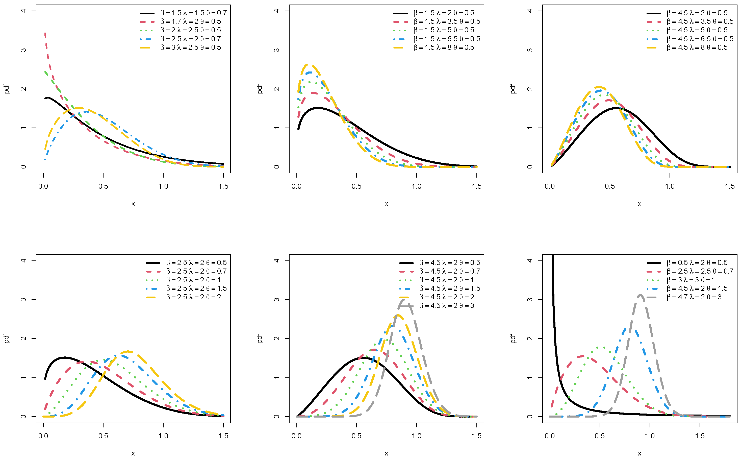
The PDF plots of the proposed SEW distribution for different parameter settings are given in Figure 1 below. From the Figure 1, it is evident that the SEW distribution can assume multiple shapes, including positively skewed, negatively skewed, and symmetric. It shows that the proposed SEW distribution may fit better to datasets that exhibit skewness, heavy-tailedness, or complex failure patterns. This makes the SEW distribution particularly useful in applications in different research fields.

2.1. Linear Expansion of the PDF of the SEW Distribution

The expansion of the PDF is often used to simplify complex mathematical expressions or analyze the behavior of a function in a specific range. This expansion, such as a Taylor or series approximation, helps in deriving insights, performing computations, or solving problems analytically. It is beneficial for statistical modeling, error analysis, and numerical simulations. Now, consider the PDF given in (6)
f S E W ( x ) = exp ( 1 ) exp ( 1 ) 1 β θ λ x β 1 exp ( λ x β ) 1 exp ( λ x β ) θ 1 × exp 1 exp ( λ x β ) θ = i = 0 j = 0 θ i + θ 1 W i , j β x β 1 exp ( 1 + j ) λ x β
where
W i , j = exp ( 1 ) exp ( 1 ) 1 θ λ ( 1 ) i + j i ! θ i + θ 1 j .
Convergence of the series representation. The infinite series representation of the SEW density is obtained from the exponential series expansion, which is absolutely convergent for all real arguments. Since 0 1 exp ( λ x β ) 1 for x > 0 , the resulting series remains absolutely convergent. Moreover, the inner summation over j is finite for each fixed i. Therefore, the density can be expressed as an absolutely convergent series for λ > 0 , β > 0 , and θ > 0 .

2.2. Moments of SEW Distribution

This section gives the rth moment, μ r , of the SEW distribution. Furthermore, important statistical measures are also obtained.
Theorem 1.
The r th moment, μ r , of the SEW distribution is given as follows:
μ r = E X r = i = 0 j = 0 θ i + θ 1 W i , j 1 ( 1 + j ) λ r β + 1 Γ r β + 1 .
Proof. 
By definition,
E X r = i = 0 j = 0 θ i + θ 1 W i , j β 0 x r x β 1 e 1 + j λ x β d x
Let y = 1 + j λ x β ; then, the r th moment of the SEW distribution is written as
E X r = i = 0 j = 0 θ i + θ 1 W i , j 1 1 + j λ r β + 1 0 y r β + 1 1 e y d y ,   = i = 0 j = 0 θ i + θ 1 W i , j 1 1 + j λ r β + 1 Γ r β + 1 .
Using the r th moment, the variance, standard deviation (SD), skewness, and kurtosis can be easily derived:
σ 2 = E X 2 μ 2   = i = 0 j = 0 θ i + θ 1 W i , j 1 1 + j λ 2 β + 1 Γ 2 β + 1 i = 0 W i 1 1 + j λ 1 β + 1 Γ 1 β + 1 2 .
The first four moments, SD, skewness (Sk), and kurtosis (Ku) of the SEW distribution are calculated for different parametric values and are given in Table 2 below.

Standard Deviation, Skewness, and Kurtosis: Analytical Interpretation

From Table 2, the following observations can be made.
Standard deviation: As the shape parameter β increases, the SD generally decreases, indicating a more concentrated distribution. For example, for λ = 1.1 and θ = 1.1 , the SD decreases from 0.4119 ( β = 2.0 ) to 0.2992 ( β = 3.0 ). Increasing θ tends to slightly increase the SD, showing that a higher θ produces longer tails and a slightly more dispersed distribution. Similarly, increasing λ tends to decrease the SD, indicating more concentrated values around the mean.
Skewness: Most parameter sets exhibit positive skewness, indicating right-skewed distributions with longer right tails. However, for larger β values ( β > 4.5 ) and moderate θ , skewness becomes negative or near-zero ( β = 5.5 , Sk = 0.104 ), indicating a slight left-skewed or nearly symmetric shape. Thus, the SEW distribution can flexibly model both right- and left-skewed data, depending on the choice of β and θ .
Kurtosis: Values greater than 3 indicate a leptokurtic (heavy-tailed) distribution, which is observed for lower β and higher θ , suggesting a higher probability of extreme values. As β increases, kurtosis approaches 3 ( β = 5.5 , Ku = 3.001 ), indicating a shape closer to a normal distribution. Therefore, the SEW distribution can flexibly capture both heavy-tailed and near-normal behaviors depending on the parameters.
These interpretations demonstrate that the SEW distribution provides flexible control over spread, skewness, and tail behavior. Parameter choices allow the modeling of datasets with concentrated or dispersed values, right- or left-skewed shapes, and light- or heavy-tailed distributions, which is particularly useful in reliability, lifetime, and extreme value applications.

2.3. Reliability Analysis

Assume X that the random variable follows the SEW distribution. Then, the survival function ( R ( x ) ), hazard rate function ( h ( x ) ), cumulative hazard function ( H ( x ) ), and reversed hazard function ( γ h ( x ) ) of the SEW distribution are as given below:
R x = 1 e x p 1 e x p 1 1 1 e x p 1 e x p λ x β θ .
h x = e x p 1 β θ λ x β 1 e x p λ x β 1 e x p λ x β θ 1 e x p 1 e x p λ x β θ e x p 1 1 e x p 1 1 e x p 1 e x p λ x β θ .
H x = ln 1 e x p 1 e x p 1 1 1 e x p 1 e x p λ x β θ .
γ h x = e x p 1 β θ λ x β 1 e x p λ x β 1 e x p λ x β θ 1 e x p 1 e x p λ x β θ 1 e x p 1 e x p λ x β θ .
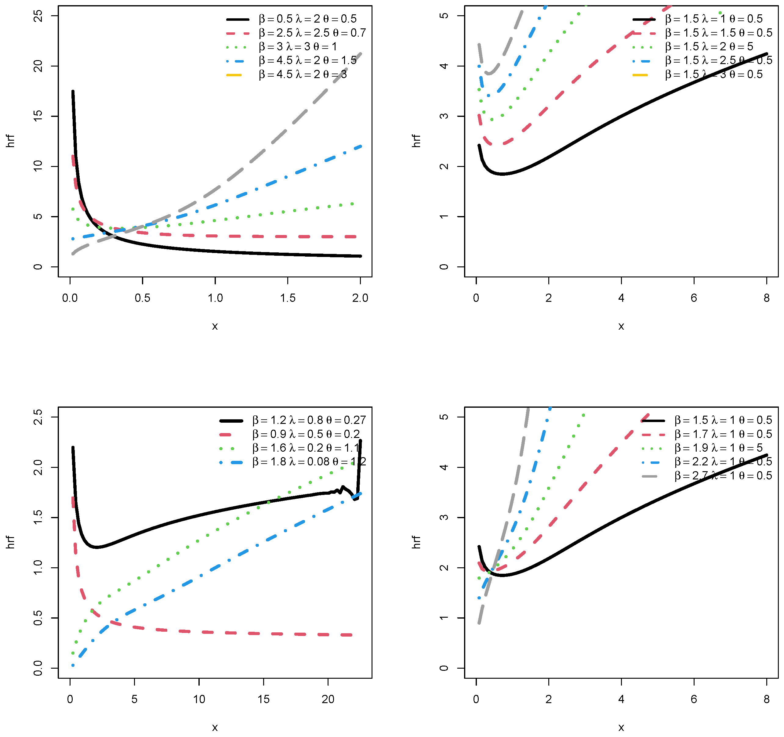
The plots of h ( x ) for different parameter settings are presented in the following Figure 2. From Figure 2, it can be seen that the proposed SEW distribution can model multiple hazard rate functions, including decreasing, increasing, and bathtub-shaped behaviors.

2.4. Quantile Function (QF) of SEW Distribution

This section focuses on deriving the QF of the SEW distribution. For the CDF of the SEW distribution, the QF is defined by q = F S E W ( x ) . Accordingly, the QF corresponding to the SEW distribution can be derived from (5) as follows:
q = e x p 1 e x p 1 1 1 e x p 1 e x p λ x β θ , e x p λ x β = 1 ln 1 e x p 1 e x p 1 1 q 1 1 θ , x β = 1 λ ln 1 ln 1 e x p 1 e x p 1 1 q 1 1 θ
Q u = ln 1 ln 1 e x p 1 1 e x p 1 u 1 1 θ 1 λ 1 β .

2.5. Lorenz and Bonferroni Curves of SEW Distribution

The Bonferroni and Lorenz curves play a significant role in various fields, such as economics and demography (see [35,36]). These curves for the SEW distribution are given as follows:
L x = 1 μ i = 0 j = 0 θ i + θ 1 W i , j 1 λ j + 1 1 + 1 β γ 1 + 1 β , j + 1 λ q β
B x = 1 μ F S E W x i = 0 j = 0 θ i + θ 1 W i , j 1 λ j + 1 1 + 1 β γ 1 + 1 β , j + 1 λ q β .

2.6. Absolute Deviations from the Mean and Median of the SEW Distribution

The mean deviation, whether it is calculated from the mean or median, is a good measure of dispersion. It provides an idea of the magnitude by which values differ from the central tendency. According to [37], it often provides a more intuitive estimate of variability than others. It is particularly useful in situations where extreme values may skew the standard deviation. The mean deviation from the mean and median of the SEW distribution is given below:
M . D m e a n = 2 μ F S E W μ 2 0 μ x f S E W x d x ,   = 2 μ F μ 2 i = 0 j = 0 θ i + θ 1 W i , j 1 λ 1 + j 1 + 1 β γ 1 + 1 β , λ 1 + j μ β
and
M . D m e d i a n = μ 2 0 M x f S E W x d x ,   = μ 2 i = 0 j = 0 θ i + θ 1 W i , j 1 λ 1 + j 1 + 1 β γ 1 β + 1 , λ 1 + j M β .

2.7. Mean Waiting Time and Mean Residual Life of the SEW Distribution

The mean waiting time defines the typical period of time that an item spends in a system before receiving service or experiencing an event. The mean residual life describes the expected remaining time until an event occurs, given that survival up to a certain point is assumed. Such measures are essential in queueing systems and reliability theory. They aid in evaluating system performance and forecasting future behavior under existing conditions. The mean waiting time and mean residual life of the SEW distribution are given below:
M W T = t 1 F x 0 t x f S E W x d x ,   = t 1 F x i = 0 j = 0 θ i + θ 1 W i , j 1 λ j + 1 1 + 1 β γ 1 + 1 β , λ j + 1 t β ,
and
M R L = 1 R x μ 0 t x f S E W x d x t ,   = 1 R x μ i = 0 j = 0 θ i + θ 1 W i , j 1 j + 1 λ 1 + 1 β γ 1 + 1 β , λ j + 1 t β t .

2.8. Renyi Entropy and Tsallis Entropy of the SEW Distribution

In order to determine the Renyi and Tsallis entropies of the SEW distribution, we need to find
0 f x r d x = 0 β θ λ e x p 1 e x p 1 1 x β 1 e x p λ x β 1 e x p λ x β θ 1 e x p 1 e x p λ x β θ r d x ,   = β θ λ e x p 1 e x p 1 1 r 0 x r β r e x p r λ x β 1 e x p λ x β r θ r e x p r 1 e x p λ x β θ d x ,
Using the series expansion e x p r 1 e x p λ x β θ = m = 0 1 m r m 1 e x p λ x β θ m m ! in (10), we get
0 f x r d x = e x p 1 e x p 1 1 β θ λ r m = 0 1 m r m m ! 0 x r β r e x p r λ x β 1 e x p λ x β r θ + θ m r d x .
Thus, using the binomial theorem, (11) can be expressed as
0 f x r d x = 1 1 r ln β θ λ e x p 1 e x p 1 1 r m = 0 j = 0 r θ + m θ r 1 m + j r i r θ + m θ r j m ! 0 x r β r e x p j + r λ x β d x .
Let j + r λ x β = y , and then x = y j + r λ 1 β . Placing this value in (12), we get
0 f x r d x = β θ λ exp ( 1 ) exp ( 1 ) 1 r m = 0 j = 0 r θ + θ m r 1 m ! ( 1 ) m + j r m r θ + θ m r j 1 ( j + r ) λ r + 1 β r β 0 y r + 1 β r β 1 e y d y , = β θ λ exp ( 1 ) exp ( 1 ) 1 r m = 0 j = 0 r θ + m θ r 1 m ! ( 1 ) m + j r m r θ + m θ r j 1 ( j + r ) λ r + 1 β r β Γ r + 1 β r β .
Using (13), the Renyi and Tsallis entropies can be computed as follows:
R p = 1 1 r ln = β θ λ e x p 1 e x p 1 1 r m = 0 j = 0 r θ + m θ r 1 m ! 1 m + j r m r θ + m θ r j 1 j + r λ r + 1 β r β Γ r + 1 β r β .
T p = 1 r 1 = β θ λ e x p 1 e x p 1 1 r m = 0 j = 0 r θ + m θ r 1 m ! 1 m + j r m r θ + m θ r j 1 j + r λ r + 1 β r β Γ r + 1 β r β .

3. Parameter Estimation of SEW Distribution via SRS and RSS

The following section deals with the development of maximum likelihood (ML) estimators for the SEW distribution under both the SRS and RSS methods. A simulation study is also conducted to assess and compare the efficiency of the proposed estimators under these two sampling methods. It is known that RSS makes use of additional information in the form of ranks and hence offers efficiency in estimation, especially for skewed and heavy-tailed distributions (see [38]). It has been seen in various research papers that RSS offers better and more reliable results for estimating parameters compared to SRS under given conditions (see [39]). Moreover, due to the flexible nature of the SEW distribution, incorporating RSS would be beneficial in improving the estimation efficiency for complex lifetime data (see [40,41]). Many authors have used ranked set samples (see [42,43,44,45,46]). However, the efficiency of SRS and RSS depends on the distribution and sample size. Hence, in this study, the results of simulations for SRS and RSS are presented to enable a comparative assessment of these two methods in terms of efficiency and reliability in estimating the parameters of the SEW distribution.

3.1. ML Estimator of SEW Distribution via SRS

Consider a random sample X 1 , X 2 , , X n drawn from the SEW distribution. The likelihood function is formulated as
L = k = 0 n e x p 1 e x p 1 1 β θ λ x β 1 e x p λ x β 1 e x p λ x β θ 1 e x p 1 e x p λ x β θ .
Hence, the log-likelihood expression for the SEW distribution based on SRS can be written as
l = ln L = ln e x p 1 e x p 1 1 n β n θ n λ n i = o n x i β 1 e x p λ x β 1 e x p λ x β θ 1 e x p 1 e x p λ x β θ   = ln e x p 1 e x p 1 1 n + n ln β + n ln θ + n ln λ + β 1 k = 1 n x i λ k = 1 n x i β     + θ 1 k = 1 n 1 e x p λ x β k = 1 n 1 e x p λ x β θ .
The partial derivatives of (14) with respect to θ , λ , and β are as follows:
l θ = n θ + k = 1 n log 1 e x p λ x β k = 1 n 1 e x p λ x β θ log 1 e x p λ x β θ , l λ = n λ k = 1 n x i β + θ 1 k = 1 n x i β e x p λ x β 1 e x p λ x β θ k = 1 n x i β e x p λ x β 1 e x p λ x β θ 1 , l β = n β k = 1 n x i β λ k = 1 n log x i + θ 1 λ k = 1 n x i β e x p λ x β log x i 1 e x p λ x β     θ λ k = 1 n 1 e x p λ x β θ 1 x i β e x p λ x β log x i .
The ML estimators of the parameters are obtained by numerically solving the following nonlinear equations: l λ = 0 , l θ = 0 , and l β = 0 .

3.2. ML Estimators of SEW Distribution via RSS

The RSS process works as follows. Assume that j represents the number of cycles, with m units selected in each, while keeping the total sample size constant. The overall sample size is n = j m . To perform the RSS procedure, the following steps are taken.
1.
First, draw m 2 items at random from the population, followed by random allocation into m subsets, with each subset containing m units.
2.
Use a simple and inexpensive method to rank the units within each set.
3.
From each ith set, for i = 1 , 2 , , m , select the unit that ranks ith.
4.
Repeat the above steps j times to obtain a final sample of size n = j m .
Let X ( i ) i c denote the ith selected observation from the ith set in the cth cycle, where i = 1 , 2 , , m and c = 1 , 2 , , j . These observations form the RSS from the SEW distribution. For simplicity, define Y i c = X ( i ) i c . For a fixed cycle c, the observations Y i c are independent and follow the PDF of the ith-order statistic. The likelihood function is then constructed based on the sample Y 1 c , Y 2 c , , Y m c .
L = c = 1 j i = 1 m m ! i 1 ! m i ! e x p 1 e x p 1 1 1 e 1 e λ x β θ i 1     1 e x p 1 e x p 1 1 1 e 1 e λ x β θ m i e x p 1 e x p 1 1 β θ λ x β 1     e x p λ x β 1 e x p λ x β θ 1 e x p 1 e x p λ x β θ .
The log-likelihood expression for the SEW distribution based on RSS can be written as
l = ln L = k m C k : m + ln x + k m log β θ λ + β 1 c = 1 j i = 1 m y i c λ i = 1 m c = 1 j y i c β     + θ 1 i = 1 m c = 1 j log 1 e x p λ y i c β i = 1 m c = 1 j 1 e x p λ y i c β θ     + i = 1 m c = 1 j i 1 e x p 1 e x p 1 1 1 e x p 1 e x p λ y i c β θ +     i = 1 m c = 1 j m i 1 e x p 1 e x p 1 1 1 e x p 1 e x p λ y i c β θ ,
where C k : m = m ! i 1 ! m i ! .
The partial derivatives of (15) with respect to θ , λ , and β are as follows:
l β = i = 1 m c = 1 j log y i c + j m β λ i = 1 m c = 1 j y i c β log y i c     λ θ i = 1 m c = 1 j Z i c log y i c + θ 1 λ i = 1 m c = 1 j e x p λ y i c β y i c β log y i c 1 e x p λ y i c β     + λ θ i = 1 m c = 1 j i 1 Z i c log y i c e x p 1 e x p λ y i c β θ 1 e x p 1 e x p λ y i c β θ     λ θ i = 1 m c = 1 j e m i e 1 Z i c log y i c e x p 1 e x p λ y i c β θ 1 e e 1 1 e x p 1 e x p λ y i c β θ ,
where 1 e x p λ y i c β θ 1 e x p λ y i c β y i c β = Z i c
l λ = i = 1 m c = 1 j y i c β + j m λ + θ 1 λ i = 1 m c = 1 j e x p λ y i c β y i c β 1 e x p λ y i c β     θ i = 1 m c = 1 j Z i c + θ i = 1 m c = 1 j i 1 Z i c e x p 1 e x p λ y i c β θ 1 e x p 1 e x p λ y i c β θ     θ i = 1 m c = 1 j e m i e 1 Z i c e x p 1 e x p λ y i c β θ 1 e x p 1 e x p 1 1 1 e x p 1 e x p λ y i c β θ ,
l θ = i = 1 m c = 1 j log 1 e λ y i c β + i = 1 m c = 1 j U i c + j m θ     + i = 1 m c = 1 j i 1 U i c e x p 1 e x p λ y i c β θ 1 e x p 1 e x p λ y i c β θ     i = 1 m c = 1 j e m i e 1 U i c e x p 1 e x p λ y i c β θ 1 e x p 1 e x p 1 1 1 e x p 1 e x p λ y i c β θ ,
where 1 e x p λ y i c β θ log 1 e x p λ y i c β = U i c .

3.3. Simulation Procedures: SRS and RSS

This section describes the simulation procedures to obtain the ML estimators of the SEW distribution under both SRS and RSS. All simulations were carried out using R software (version 4.1.2). The performance of the estimators is evaluated based on the mean squared error (MSE).
  • The simulation procedure follows the steps below.
    1.
    For each sampling scheme (SRS and RSS), generate a sample of size n = 30 , 50 , 70 using the proposed distribution with selected parameter combinations. In the case of RSS, appropriate set size m and number of cycles j are chosen such that n = m j .
    2.
    The following parameter settings are used in the simulations:
    ( λ = 0.8 , β = 2.5 , θ = 0.5 )
    ( λ = 1.6 , β = 3.0 , θ = 0.5 )
    3.
    For each combination, we compute the ML estimators of the parameters under both the SRS and RSS schemes.
    4.
    Repeat steps 1–3 for N = 100 iterations. For each case, calculate the MSE of the estimated parameters over the repetitions.
    5.
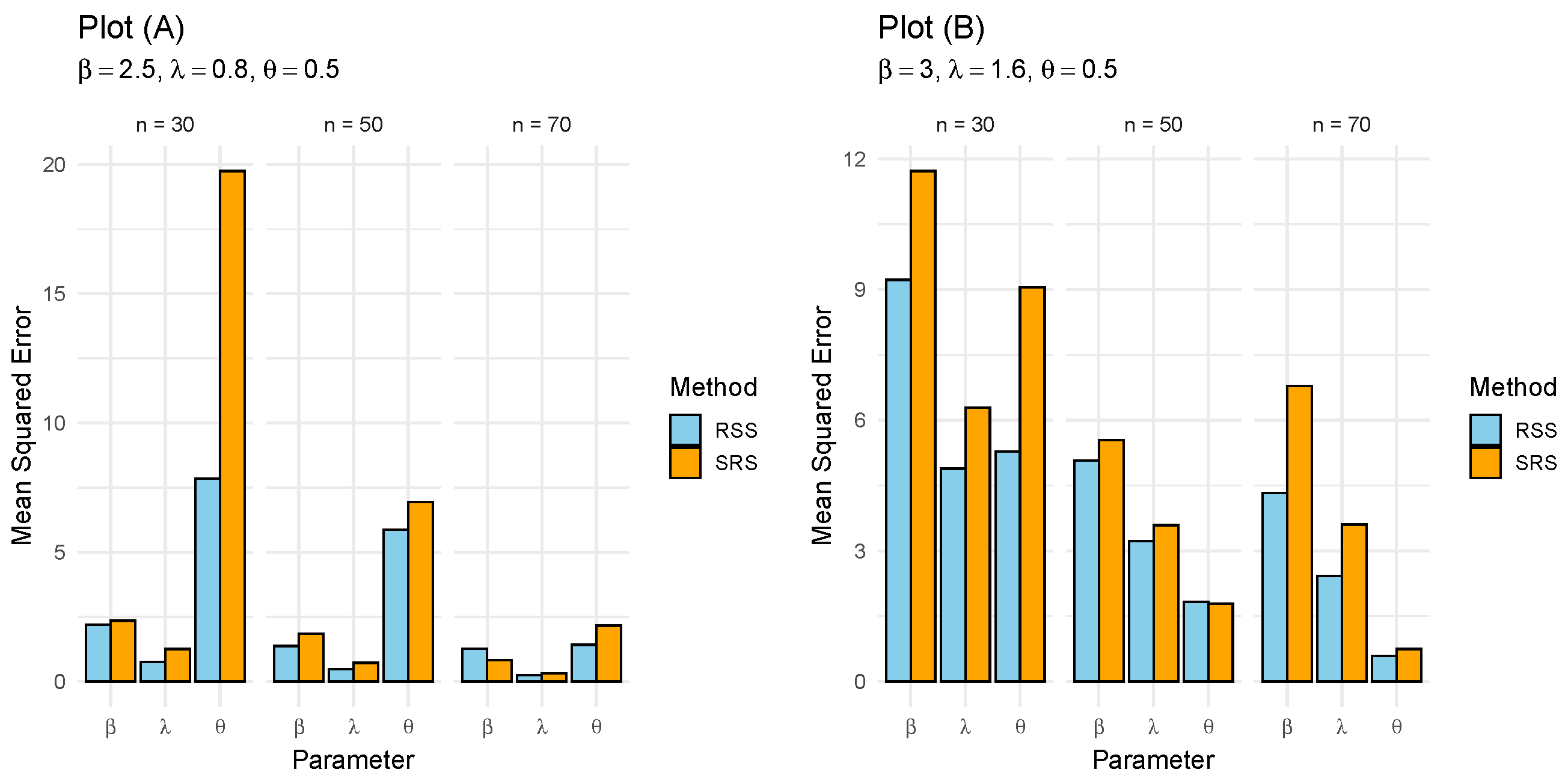
    The computed MSE values for different scenarios are summarized graphically in Figure 3 below.
Figure 3 describes the behavior of the MSE for the SEW distribution parameters with the help of SRS and RSS for different sample sizes. From the results, a clear trend of decreasing mean squared errors is visible as the sample size increases from 30 to 70. From the results shown in Plot (A), it is clear that RSS performs relatively better than SRS for the SEW model parameters, as the MSE is lower for all parameters. However, for the sample size n = 70 , SRS performs slightly better for the parameter β , even though RSS performs better for all parameters. From the results in Plot (B), we can see that RSS performs better for all parameters, whereas SRS performs slightly better for the parameter θ for the sample size n = 70 . From the results, it is clear that RSS performs better than SRS for the given SEW model.

4. Estimation of Parameters Through Different Methods of Estimation

The parameters of the SEW distribution are estimated using seven different classical and alternative methods, including maximum likelihood estimation (MLE), least squares estimation (LSE), weighted least squares estimation (WLSE), maximum product spacing estimation (MPSE), Cramér–von Mises estimation (CRVME), Anderson–Darling estimation (ADE), and right-tail Anderson–Darling estimation (RADE). The details of these methods can be seen in [47].
The ML estimators of the parameters are obtained by differentiating the log-likelihood function with respect to each parameter. Θ = ( β , λ , θ ) and solving the resulting system of equations:
( Θ ) β = 0 , ( Θ ) λ = 0 , ( Θ ) θ = 0 .
The LSE and WLSE of the parameters are obtained by minimizing
O ( β , λ , θ ) = i = 1 n ν i F ( x i ; β , λ , θ ) i n + 1 2 ,
where ν i = 1 for LSE and ν i = ( n + 1 ) 2 ( n + 2 ) i ( n i + 1 ) for WLSE. The estimating equations are given by
i = 1 n F ( x i ; β , λ , θ ) i n + 1 δ s ( x i ) = 0 , s = 1 , 2 , 3 ,
where δ s ( x i ) are the derivatives of the CDF with respect to the parameters.
The partial derivatives OF the SEW distribution are obtained as follows:
F S E W ( x ) β = e e 1 exp 1 e λ x β θ θ 1 e λ x β θ 1 λ x β ln ( x ) e λ x β ,
F S E W ( x ) λ = e e 1 exp 1 e λ x β θ θ 1 e λ x β θ 1 x β e λ x β ,
F S E W ( x ) θ = e e 1 exp 1 e λ x β θ 1 e λ x β θ ln 1 e λ x β .
MPSE is an alternative approach to MLE. The uniform spacing of a random sample of size n is defined by
H ( β , λ , θ ) = i = 1 n + 1 log D i ,
where
D i = F ( x i : n ) F ( x i 1 : n ) , F ( x 0 : n ) = 0 , F ( x n + 1 : n ) = 1 .
The MPSE of the parameters is obtained by solving
i = 1 n + 1 1 D i δ s ( x i : n ) δ s ( x i 1 : n ) = 0 , s = 1 , 2 , 3 .
CRVME minimizes the distance between empirical and theoretical CDFs:
C ( β , λ , θ ) = 1 12 n + i = 1 n F ( x i : n ) 2 i 1 2 n 2 ,
with estimating equation
i = 1 n F ( x i : n ) 2 i 1 2 n δ s ( x i : n ) = 0 .
ADE is obtained by minimizing
A ( β , λ , θ ) = n 1 n + i = 1 n ( 2 i 1 ) ln F ( x i : n ) + ln S ( x i : n ) ,
leading to the system
i = 1 n ( 2 i 1 ) δ s ( x i : n ) F ( x i : n ) + δ s ( x i : n ) S ( x i : n ) = 0 , s = 1 , 2 , 3 .
Finally, RADE is obtained by solving
i = 1 n δ s ( X i : n ) 2 i 1 2 n F ( X i : n ; β , λ , θ ) = 0 , s = 1 , 2 , 3 .

Simulation Study

The rationale for adopting different estimation techniques for the estimation of the parameters of the proposed SEW distribution is to provide a comprehensive comparison of the relative performance of these estimation techniques, since the relative performance of the estimators may vary depending on the method adopted for estimation. For evaluating and comparing the relative performance of the adopted estimators, the Monte Carlo simulation method is used for SRS. The relative performance of the estimators is compared based on the MSE, average absolute bias (AB), and mean relative error (MRE). These performance measures are defined as
M S E = 1 N i = 1 N ( δ ^ i δ ) 2 ,
A B = 1 N i = 1 N δ ^ i δ ,
M R E = 1 N i = 1 N δ ^ i δ δ ,
where δ = ( β , λ , θ ) .
  • Different sample sizes, such as n = 30 , 50 , 100 , 150 , 200 , 300 , and different parametric values, such as δ = ( 2 , 1.5 , 1.3 ) , ( 1.5 , 1.8 , 1.6 ) , ( 1.2 , 2 , 2.3 ) , ( 1.8 , 1.7 , 1.6 ) , are considered for the simulation process. For each case, N = 5000 Monte Carlo replications are conducted through the quantile function of the SEW distribution in the R (version 4.1.2). The main aim of this simulation is to check the accuracy and efficiency of the different estimators for different sample sizes and to find the best estimation method for the SEW model under SRS. Superscripts denote ranking of estimators based on performance (1 = best, higher numbers indicate lower performance). The simulation results are arranged in Table 3, Table 4, Table 5 and Table 6 given below.
  • The simulation outcomes in Table 3, Table 4, Table 5 and Table 6 demonstrate the performance of the different estimation procedures in terms of the AB, MSE, and MRE for sample sizes n = 30 , 50 , 100 , 150 , 200 , and 300. The ranks of each procedure, summed to provide a combined measure of performance, were obtained based on the AB, MSE, and MRE. The outcomes of the simulation reveal that the accuracy of estimation increases with an increase in sample size, validating the consistency of the estimators and also highlighting the differences in the efficiency and stability of the estimators. Table 7 presents a summary of the overall ranking of the estimation procedures for all parameter combinations and sample sizes. MPSE appears to be the most promising estimator, followed by WLSE and MLE, which show better accuracy in their estimation results. The MPSE, MLE, and ADE methods show moderate performance, whereas OLSE, WLSE, and CVME show poor performance in estimation due to higher bias and variability in the results. R A D E shows superior results, providing the most reliable estimations.

5. Distribution of Order Statistics from SEW Distribution

Order statistics have a key role in the theory and application of statistics. They are important in studying the behavior of the extremes (minimum and maximum), medians, and percentiles of a dataset. They find extensive application in reliability analysis, life testing, and nonparametric inference, where minimal assumptions are made regarding underlying distributions. Order statistics also provide the basis for defining robust estimators and tolerance intervals. In the analysis of censored data, they are more efficient and flexible than basic random samples (see [48,49]). Additionally, their distributional properties assist in describing probability distributions, as well as in hypothesis testing (see [50]).

5.1. Univariate Case

Let Y 1 , Y 2 , , Y n be a random sample generated from the SEW distribution. The sample values, once arranged in ascending order, are denoted by Y 1 : n , Y 2 : n , . . . , Y n : n . The PDF corresponding to the smallest and largest observations in a sample drawn from the SEW distribution can be expressed as follows:
f 1 : n y = n β θ λ y β 1 e x p λ y β 1 e x p λ y β θ 1 e x p 1 e x p λ y β θ     e x p 1 e x p 1 1 1 e x p 1 e x p 1 1 1 e x p 1 e x p λ y β θ n 1 ,
f n : n y = n e x p λ y β 1 e x p λ y β θ 1 e x p 1 e x p λ y β θ     e x p 1 e x p 1 1 β θ λ y β 1 e x p 1 e x p 1 1 1 e x p 1 e x p λ y β θ n 1 .
Theorem 2.
The PDF of the r th -order statistic, f r : n ( y ) , for the SEW distribution is given by
f r : n x = C r : n β θ λ W ψ x β 1 e λ + λ l x β ,
where W ψ = i = o n r j = 0 r + i 1 k = 0 l = 0 θ k + θ 1 1 i + j + k + l 1 + j k k ! n r i r + i 1 j θ k + θ 1 l e e 1 r + i .
Proof. 
First, it should be noted that the PDF of the r th -order statistic can be written as
f r : n y = C r : n i = o n r 1 i n r i F S E W y r + i 1 f S E W y .
Using (5) and (6) in the above equation, we get
f r : n y = C r : n i = o n r 1 i n r i e x p 1 e x p 1 1 1 e x p 1 e x p λ y β θ r + i 1     e x p 1 e x p 1 1 β θ λ y β 1 e x p λ y β 1 e x p λ y β θ 1 e x p 1 e x p λ y β θ .
By using binomial expansion, the PDF of the r th -order statistic from the SEW distribution can be written as,
f r : n y = C r : n β θ λ i = o n r j = 0 r + i 1 k = 0 l = 0 θ k + θ 1 1 i + j + k + l 1 + j k k ! n r i r + i 1 j θ k + θ 1 l     e x p 1 e x p 1 1 r + i y β 1 e x p λ + λ l y β .

p t h Moment of Order Statistics

The p t h moment of the order statistics from the SEW distribution can be derived as follows.
We know that
μ r : n p = C r : n + y p f r : n y d x = C r : n β θ λ W ψ 0 y p y β 1 e x p λ + λ l y β d x .
Making the substitution z = λ + λ l y β , we find that
μ r : n p = C r : n θ λ W ψ 1 λ + λ l p β + 1 0 z p β + 1 1 e z d x   = C r : n θ λ W ψ 1 λ + λ l p β + 1 Γ p β + 1 .
where Γ . is the gamma function.

5.2. Reversed Order Statistics

Reversed order statistics play a fundamental role in statistical theory and practice. Reversed order statistics, which consist of ordering data in decreasing order, find application in early failure studies, left-censored data modeling, and reversed hazard rate studies within survival analysis. For a detailed explanation of order statistics, including reversed order statistics, their theoretical background, their distributions, and their applications in inference and reliability analysis, see [48,51]. They are particularly useful for examining instances where data are listed in descending order, such as in ranking the scores of students from highest to lowest, listing cities based on population, and so on.
Let Y 1 , Y 2 , . . . , Y n be a random sample of size n from the SEW distribution. The PDF of the reversed order statistics is written as
f r r e : n y = C r : n F S E W y n r 1 F S E W y r 1 f y ,
where C r : n = n ! r 1 ! n r !
Utilizing (5) and (6), the PDFs for the smallest ( r = 1 ) and largest ( r = n ) reversed order statistics can be directly derived from (24) and are expressed, respectively, as follows:
f 1 r e : n y = n e x p 1 e x p 1 1 β θ λ y β 1 e x p λ y β 1 e x p λ y β θ 1     e x p 1 e x p λ y β θ e x p 1 e x p 1 1 1 e x p 1 e x p λ y β θ n 1 ,
f n : r e n y = n e x p 1 e x p 1 1 β θ λ y β 1 e x p λ y β 1 e x p λ y β θ 1     e x p 1 e x p λ y β θ 1 e e 1 1 e x p 1 e x p λ y β θ n 1 .
Theorem 3.
The P D F and C D F of the SEW distribution, respectively, can be obtained. The P D F of the r t h reversed order statistic, say f r r e : n x , is given by
f r : n y = C r : n β θ λ i = o r 1 A i y β 1 e x p λ + λ l y β .
where
A i = j = 0 n r i k = 0 l = 0 θ k + θ 1 1 k + i + j + l 1 + j k k ! r 1 i n r i j     θ k + θ 1 l e x p 1 e x p 1 1 n r i + 1 .
Proof. 
Moreover, (24) may also be written in the following form:
f r r e : n x = C r : n i = o r 1 1 i n r i e x p 1 e x p 1 1 1 e x p 1 e x p λ y β θ n r i     e x p 1 e x p 1 1 β θ λ y β 1 e x p λ y β 1 e x p λ y β θ 1 e x p 1 e x p λ y β θ .
By using binomial expansion, we get
1 e x p 1 e x p λ y β θ n r i = j = 0 n r i 1 j n r i j e x p j 1 e λ y β θ ,
and
e x p 1 + j 1 e λ y β θ = k = 0 1 k 1 + j k k ! 1 e λ y β θ k
By using (30), (28), and binomial expansion, we get
1 e λ x β θ k + θ 1 = l = 0 θ k + θ 1 1 l θ k + θ 1 l e l λ x β
By combining (28)–(30) and (31), we get (24). In addition, we can write
f r r e : n x = C r : n β θ λ i = o r 1 j = 0 n r i k = 0 l = 0 θ k + θ 1 1 i + j + k + l 1 + j k k ! r 1 i n r i j     θ k + θ 1 l e x p 1 e x p 1 1 n r i + 1 y β 1 e λ + λ l y β

p t h Moment of Reversed Order Statistics

The p t h moment of the r t h reversed order statistics for p = 1 , 2 , . . . , denoted by μ r r e : n p , is given by
μ r : n p = C r : n θ λ i = o r 1 A i 1 λ + λ l p β + 1 Γ p β + 1 .
Proof. 
From (27), the p t h Moment of Reversed Order Statistics can be define as
μ r r e : n p = C r : n + y p f r : n y d x = C r : n β θ λ i = o r 1 A i 0 y p y β 1 e λ + λ l y β d x .
Making the substitution z = λ + λ l x β , we find that
μ r r e : n p = C r : n θ λ i = o r 1 A i 1 λ + λ l p β + 1 0 z p β + 1 1 e z d x   = C r : n θ λ i = o r 1 A i 1 λ + λ l p β + 1 Γ p β + 1 .

5.3. Upper Record Statistics of SEW Distribution

Records are essential in various practical fields, such as meteorological data, athletic performance metrics, financial datasets, and material strength observations. Ref. [52] explored the potential of employing upper record values in statistical analysis. The C D F and P D F of the SEW distribution, respectively, can be obtained. Moreover, we define Y i : n as the i th -order statistic, as introduced earlier.
For a fixed integer k 1 , define the sequence U k ( n ) for n 1 by setting U k ( 1 ) = 1 , and, for n 2 , U k ( n + 1 ) = min j > U k ( n ) : Y j : j + k 1 > Y U k ( n ) : U k ( n ) + k 1 . We define the associated value Y n ( k ) as Y n ( k ) = Y U k ( n ) : U k ( n ) + k 1 , n 1 .
The random variable Y n r is called the r t h upper record statistic. Then, in full generality, the PDF of Y n k is readily written as
f r u r : n y = 1 n 1 ! ln 1 F S E W y n 1 1 F S E W y r 1 f S E W y .
The density function of the r t h upper record statistic, say f r u r : n y , is given by
f r u r : n y = β θ λ i = o H i y β 1 e λ + λ m y β
where
H i = j = 0 r 1 k = 0 i + j l = 0 m = 0 θ l + θ 1 1 i + j + k + l + m r 1 j i + j k θ l + θ 1 m 1 + k l k ! 1 n i 1 ! i ! l ! e x p 1 e x p 1 1 i + j + 1
Proof. 
The Equation (33) can be written as
f r u r : n y = 1 n 1 ! i = o 1 i n 1 ! n i 1 ! i ! j = o r 1 r 1 j F S E W y i + j f S E W y .
Using Equations (5) and (6), we have
f r u r : n y = i = o j = o r 1 1 i + j β θ λ y β 1 e x p λ y β n i 1 ! i ! e x p 1 e x p 1 1 r 1 j 1 e x p λ y β θ 1     e x p 1 e x p 1 1 1 e x p 1 e x p λ y β θ i + j e x p 1 e x p λ y β θ .
By using binomial expansion, we get (35). In addition, we can write
f r u r : n y = i = o j = 0 r 1 k = 0 i + j l = 0 m = 0 θ l + θ 1 1 i + j + k + l + m r 1 j i + j k θ l + θ 1 m     1 + k l k ! 1 n i 1 ! i ! l ! e x p 1 e x p 1 1 i + j + 1 y β 1 e x p λ + λ l y β   = β θ λ i = o H i y β 1 e x p λ + λ l y β

p t h Moment of Upper Record Statistics

The p t h moment of the r t h upper record statistics is derived in the following theorem.
Theorem 4.
The p t h moment of the r t h upper record statistics for p = 1 , 2 , . . . , denoted by μ y n r p , is given by
μ r u r : n p = θ λ i = o H i 1 λ + λ m p β + 1 Γ p β + 1
Proof. 
From (34), the p t h Moment of Upper Record Statistics can be expressed as
μ r u r : n p = C r : n + y p f r : n y d x = β θ λ i = o H i 0 y p y β 1 e x p λ + λ l y β d x .
Making the substitution z = λ + λ m y β , we find that
μ r u r : n p = θ λ i = o H i 1 λ + λ m p β + 1 0 z p β + 1 1 e z d x   = θ λ i = o H i 1 λ + λ m p β + 1 Γ p β + 1 .

6. Applications

  • The first dataset represents the number of millions of revolutions completed by each of 23 ball bearings before experiencing failure during an endurance test [53]. The recorded values are presented as follows. Data I: 17.88, 28.92, 33.00, 41.52, 42.12, 45.60, 51.84, 51.96, 54.12, 55.56, 67.80 68.64, 68.64, 84.12, 93.12, 98.64, 105.12, 105.84, 127.92, 128.04, 174.40.
    Data 2: The second dataset represents 101 cases of progressed acute myelogenous leukemia registered at the International Bone Marrow Transplant Registry (see [54]). The data are as follows. Data II: 0.030, 0.493,0.855, 1.184, 1.283, 1.480, 1.776, 2.138, 2.500, 2.763, 2.993, 3.224, 3.421, 4.178, 4.441, 5.691, 5.855, 6.941, 6.941, 7.993, 8.882, 8.882, 9.145, 11.480, 11.513, 12.105, 12.796, 12.993, 13.849, 16.612, 17.138, 20.066, 20.329, 22.368, 26.776, 28.717, 28.717, 32.928, 33.783, 34.211, 34.770, 39.539, 41.118, 45.033, 46.053, 46.941, 48.289, 57.401, 58.322, 60.625, 0.658, 0.822, 1.414, 2.500, 3.322, 3.816, 4.737, 4.836, 4.934, 5.033, 5.757, 5.855, 5.987, 6.151, 6.217, 6.447, 8.651, 8.717, 9.441, 10.329, 11.480, 12.007, 12.007, 12.237, 12.401, 13.059, 14.474, 15.000, 15.461, 15.757, 16.480, 16.711, 17.204, 17.237, 17.303, 17.664, 18.092, 18.092, 18.750, 20.625, 23.158, 27.730, 31.184, 32.434, 35.921, 42.237, 44.638, 46.480, 47.467, 48.322, 56.086.
    The third dataset corresponds to unemployment claim data (see [55]). This dataset consists of 58 bounded observations representing unemployment claim rates in proportion form. The observed data are as follows. Data III: 0.823, 0.864, 0.816, 0.841, 0.831, 0.833, 0.894, 0.869, 0.866, 0.860, 0.837, 0.826, 0.804, 0.809, 0.758, 0.770, 0.778, 0.707, 0.814, 0.825, 0.906, 0.924, 0.927, 0.920, 0.770, 0.544, 0.550, 0.608, 0.630, 0.650, 0.820, 0.873, 0.900, 0.916, 0.899, 0.862, 0.695, 0.650, 0.751, 0.862, 0.702, 0.530, 0.764, 0.898, 0.897, 0.908, 0.902, 0.879, 0.645, 0.739, 0.765, 0.803, 0.708, 0.669, 0.561, 0.579, 0.701, 0.839.
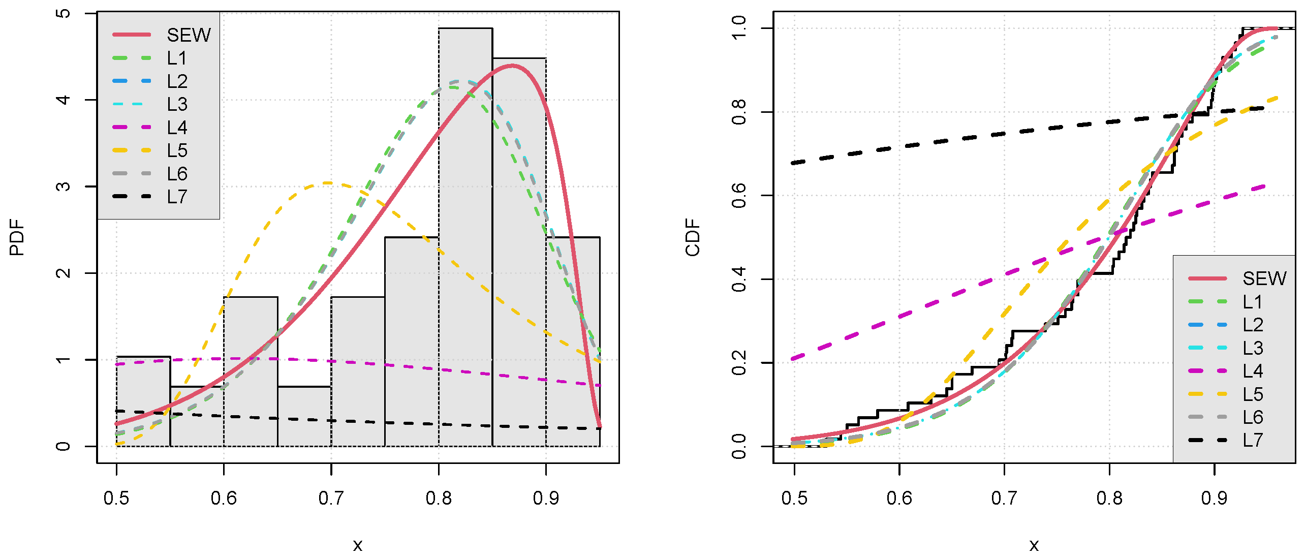
    In this study, the proposed SEW model is compared with well-known and competitive lifetime models to assess its flexibility and potential for modeling real-life data. For comparison purposes, we use a new modification of the Weibull distribution (L1) by [4], the additive Weibull model (L2) by [56], the Beta-Weibull model (L3) by [6], a new technique of adding a parameter to the Weibull distribution (L4) by [57], the inverse Weibull distribution (L5) by [58], the Burr family of cumulative frequency functions (L6) by [59], and the log-transformed generalized family of distributions (L7) by [60]. The comparison is carried out on the basis of well-established goodness-of-fit criteria such as the Akaike information criterion ( A I C ), Bayesian information criterion ( B I C ), corrected Akaike information criterion ( C A I C ), and Hannan–Quinn information criterion ( H Q I C ). Additionally, the traditional measures of the Cramér–von Mises statistic W, Anderson–Darling statistic A, Kolmogorov–Smirnov statistic K S , and p-value are used. For the descriptive analysis of the datasets, graphical tools such as the T T T plot, boxplot, kernel density, and violin plot are also employed.
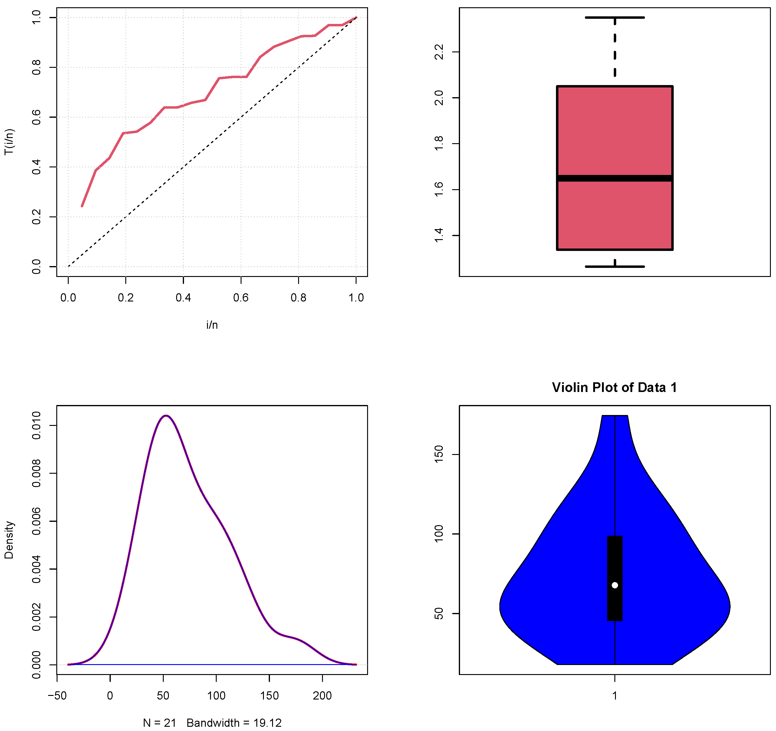
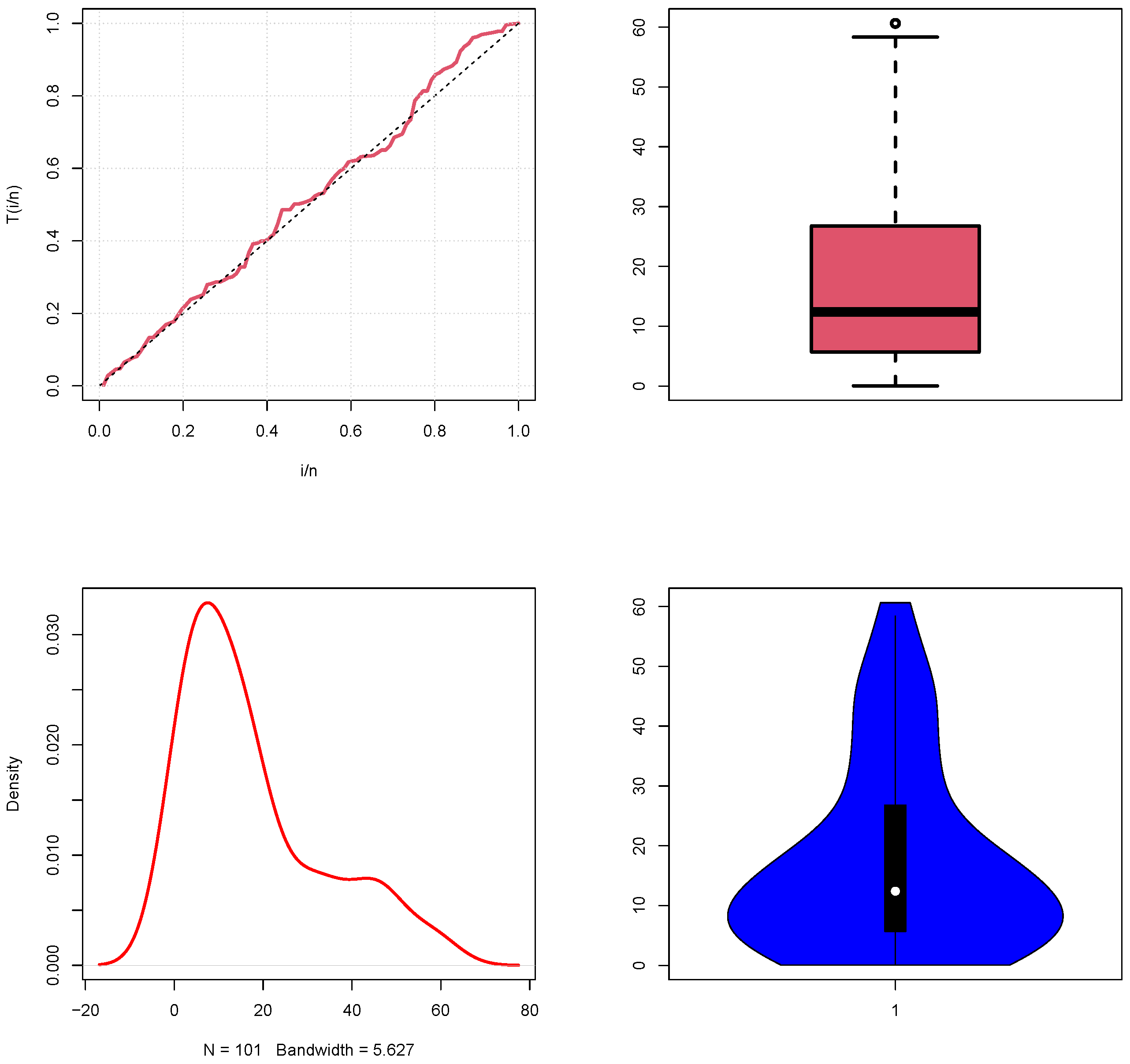
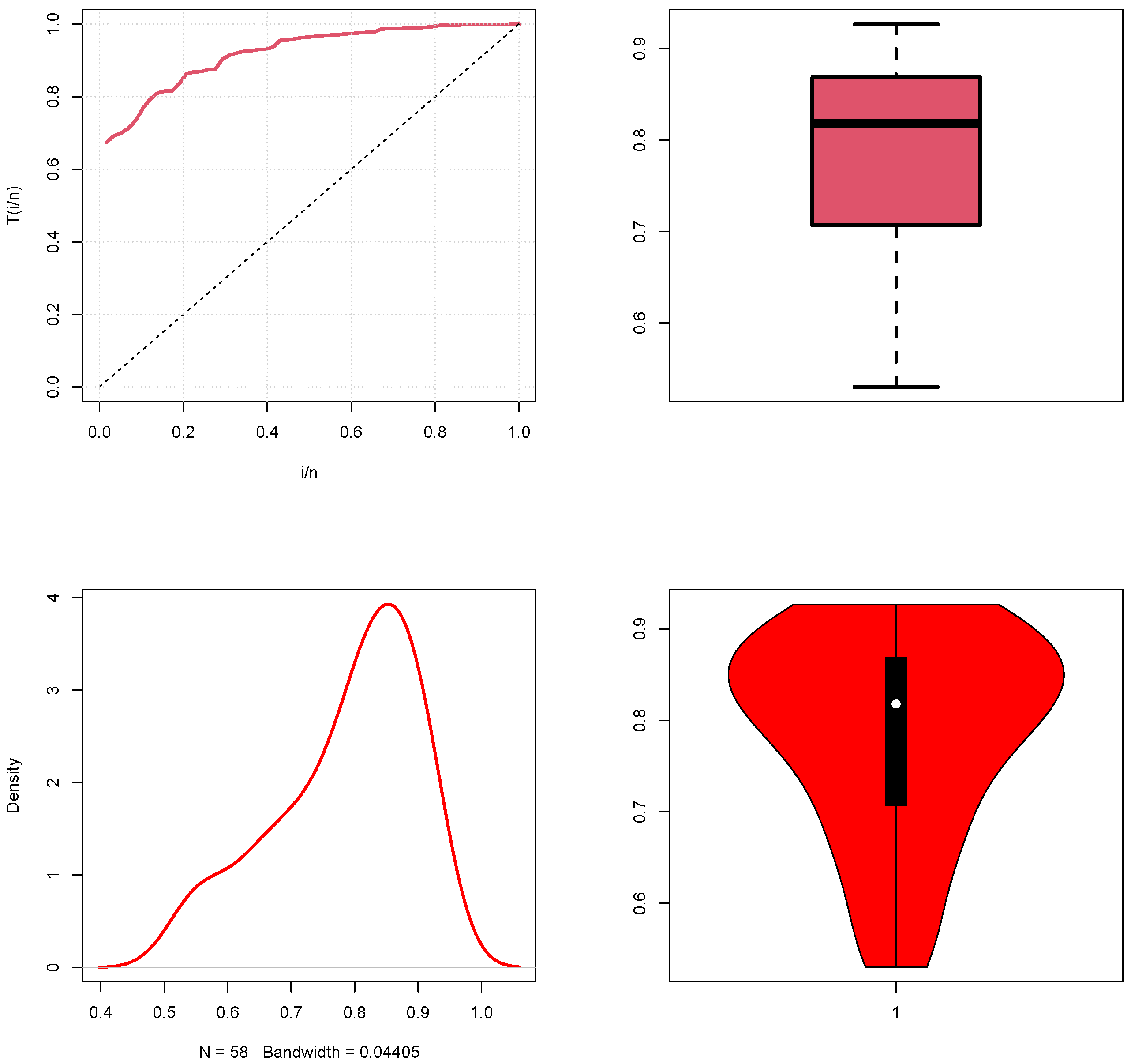
  • The graphs plotted for the three datasets are shown in Figure 4, Figure 5 and Figure 6. According to Figure 4, the first dataset yields a graph with an increasing trend, which implies that there is an increasing hazard rate. The boxplot and density plot provide additional information about minimal deviations on the right side, which implies stability. On the other hand, the second dataset, as presented in Figure 5, has an approximately linear shape in the TTT plot, which means that the dataset has a constant hazard rate. However, it is evident that there is wide dispersion, with the possibility of outliers, and that there is a right-skewed distribution in the density plot. From Figure 6, the third dataset has an increasing TTT plot, implying an increasing hazard rate, while the boxplot and kernel density have left-skewed.
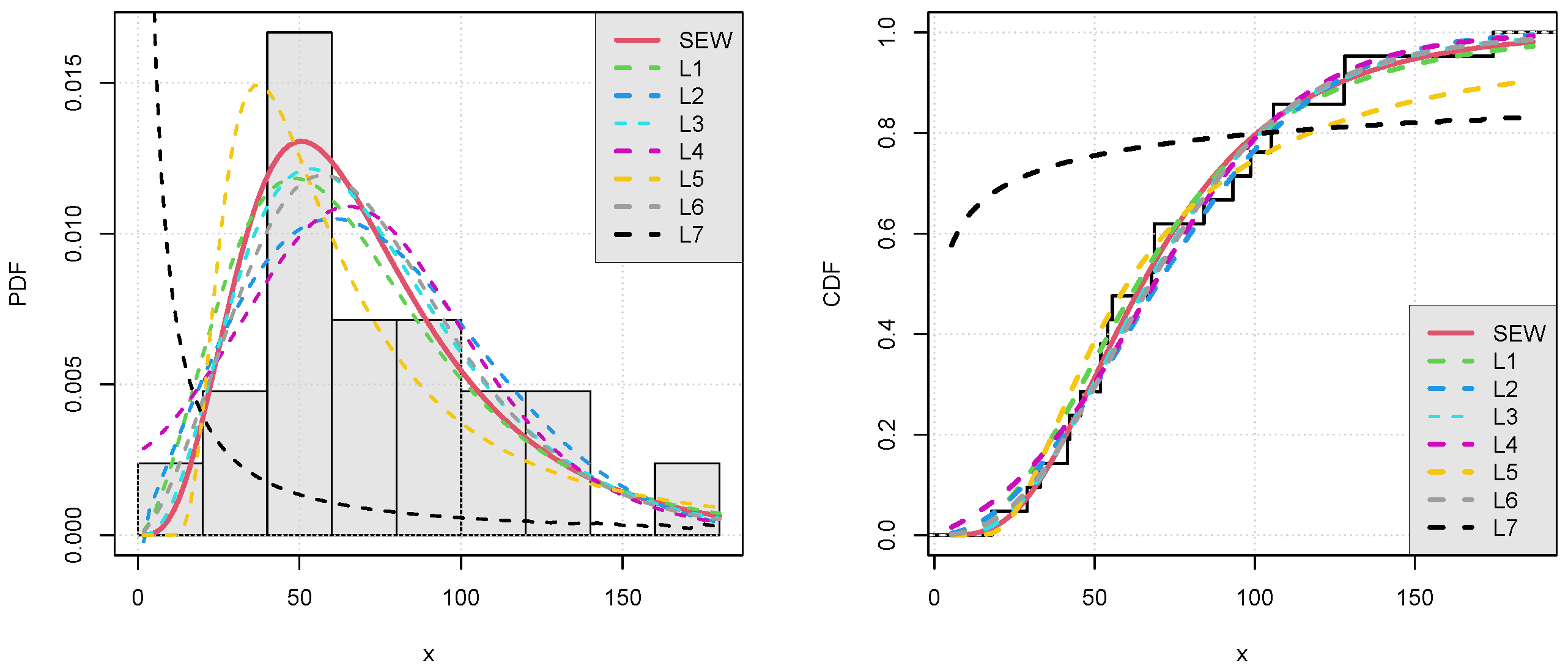
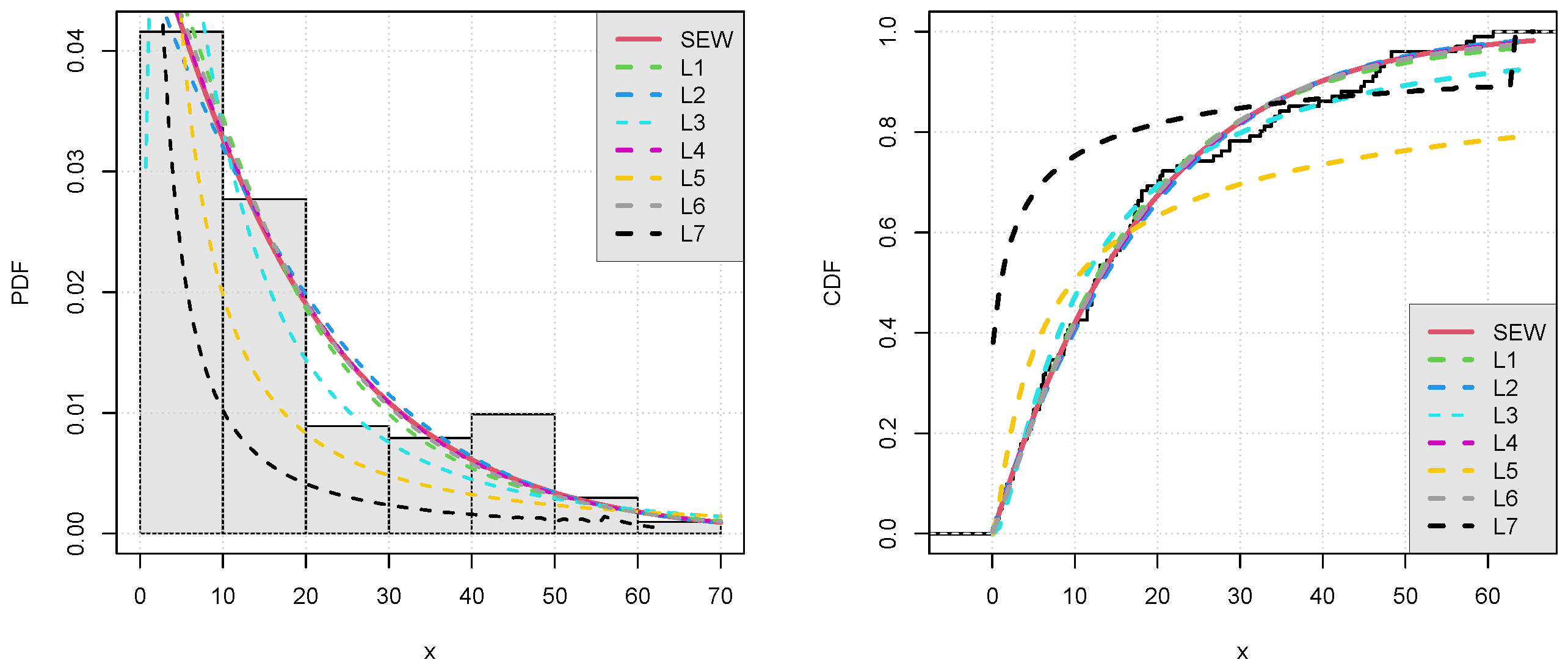
  • The practical applicability and efficacy of the proposed SEW model are demonstrated by employing the model on real-life datasets, and the results are presented in terms of the goodness-of-fit statistics, as given in Table 8, Table 9 and Table 10 and likelihood estimates and standard errors, as given in Table 11, Table 12 and Table 13. Whereas the fit of the proposed SEW model is further demonstrated by Figure 7, Figure 8 and Figure 9. It can be seen from Table 8 that the SEW model significantly outperforms the other models in terms of the log-likelihood and information criteria, including the AIC, CAIC, BIC, and HQIC, on Dataset 1. In addition, L1–L6 display comparatively poorer performance than the SEW model in fitting Dataset 1, and L7 shows an extremely poor fit as revealed by large KS values and an almost zero p-value, as evidenced in Figure 7. On Dataset 2, the SEW model exhibits strong fitting and reliability, while L4 and L6 show relative superiority in comparison with the other models, but they are still somewhat inferior to the SEW model, and L3, L5, and L7 provide a poor fit because of their large KS statistics and small p-values, as shown in Figure 8. Finally, for Dataset 3, it can be seen from Table 10 that the SEW model displays an excellent fit in terms of the maximum log-likelihood and minimal information criteria, whereas L1–L3 and L6 demonstrate moderate fitting and L4 and L7 show poor fitting for Dataset 3, as evident from Figure 9. Moreover, Table 11, Table 12 and Table 13 shows that the standard errors are relatively small, which confirms the reliability and stability of the proposed model. Therefore, based on three Dataset, the SEW model demonstrates better performance and greater estimation efficiency compared to the competing models.
  • From the above analysis, we can conclude that the proposed SEW model is better than the compared models based on statistical measures such as the log-likelihood, information criteria, and goodness of fit. Most of the existing models are either incapable of capturing the underlying distribution or offer poor goodness of fit, especially when considering the p-values and KS statistics, while the proposed model shows stability and flexibility across all datasets under study. Finally, from the above, it can be concluded that the proposed SEW model is highly efficient and effective, as it offers better statistical performance and superior goodness of fit compared to all other available models.

7. Actuarial Measures

Actuarial measures are of vital importance in the assessment of risk and financial decision-making. In insurance and reliability theory, the actuarial measures of Value at Risk (VaR) and Tail Value at Risk (TVaR) are the most commonly used risk assessment tools to measure loss and evaluate extreme risk situations. Graph-based reliability evaluation methods have been proposed to simplify reliability calculations in complex systems (see [61]). The importance of these actuarial measures has been discussed in the literature in the context of uncertainty and tail risk behavior (see [62,63]).

7.1. Value at Risk

Value at Risk (VaR), also known as quantile risk, is widely recognized as a fundamental measure of financial market risk. It is frequently employed in business and financial decision-making, particularly in situations involving uncertainty related to global markets, commodity pricing, or changes in regulatory or government policies, all of which can have a notable impact on a firm’s profitability.
VaR measures the maximum potential loss in the worth of an investment or portfolio within a given period, with a specified level of confidence, usually 90%, 95%, or 99%. Quantitatively, VaR is equivalent to the q th quantile of the CDF of a random variable x. In the case where x follows the SEW distribution, the VaR can be expressed in terms of a closed-form quantile function derived from its CDF. Assuming that the random variable X follows the SEW distribution, the VaR can be expressed as
V a R q = ln 1 ln 1 e 1 e q 1 1 θ 1 λ 1 β

7.2. Expected Shortfall

Expected shortfall (ES) is a widely used risk measure in finance that extends beyond the Value at Risk (VaR) framework, as introduced by [64]. ES estimates the expected average loss that may occur in the worst-case scenario—specifically, those beyond the VaR threshold. Unlike VaR, which only provides a cut-off point for losses at a given confidence level, ES offers additional insight into the magnitude of potential extreme losses. This characteristic makes ES particularly useful for managing and understanding tail risk in highly volatile financial markets. It is defined by the following expression:
E S q x = 1 q 0 q V a R x d x

7.3. Tail Value at Risk

Tail Value at Risk (TVaR) is an important risk measure in finance and insurance. Compared to VaR, TVaR provides more detailed information about the magnitude of extreme losses. For this reason, it is particularly useful in assessing and managing tail risks associated with high-impact events. By using (7) in (39), the Tail Value at Risk can be obtained as
T V a R q x = 1 1 q V a R q x f x d x
Let X S E W β , θ , λ , for 0 < V < 1 ; then, the Tail Value at Risk (TVaR) is given by
T V a R q x = 1 1 q i = 0 W i γ 1 β + 1 , 1 + j λ V a R q β 1 + j λ 1 β + 1

7.4. Tail Variance

Tail variance (TV) is a key risk metric that measures the range of losses exceeding the VaR threshold. While ES focuses on the average loss within the tail, TV captures the spread or dispersion of extreme losses. It indicates the degree of instability or uncertainty in worst-case scenarios. This makes TV a valuable tool for understanding the risk of extreme but adverse financial outcomes.
T V q x = E X 2 | X > x q T V a R q x 2
Let I = E X 2 | X > x q , and
I = 1 1 q V a R q x 2 f x d x
Let X S E W θ , β , λ for 0 < V < 1 ; then, I is given via (41) by
T V a R q x = 1 1 q i = 0 W i γ 1 β + 1 , 1 + j λ V a R q β 1 + j λ 1 β + 1
using (40) in (41), we obtain the expression for tail variance for the SEW model.

7.5. Tail Variance Premium

Tail variance premium (TVP) is an important risk measure that incorporates both the central tendency and dispersion. TVP is designed to evaluate the spread of extreme losses occurring beyond a certain threshold—specifically, in the right tail of the distribution. By accounting for both the average and the variability of tail losses, TVP offers a more comprehensive view of risk. For this reason, it is particularly suitable for analyzing large and infrequent financial losses.
T V P q X = T V a R q + δ T V q
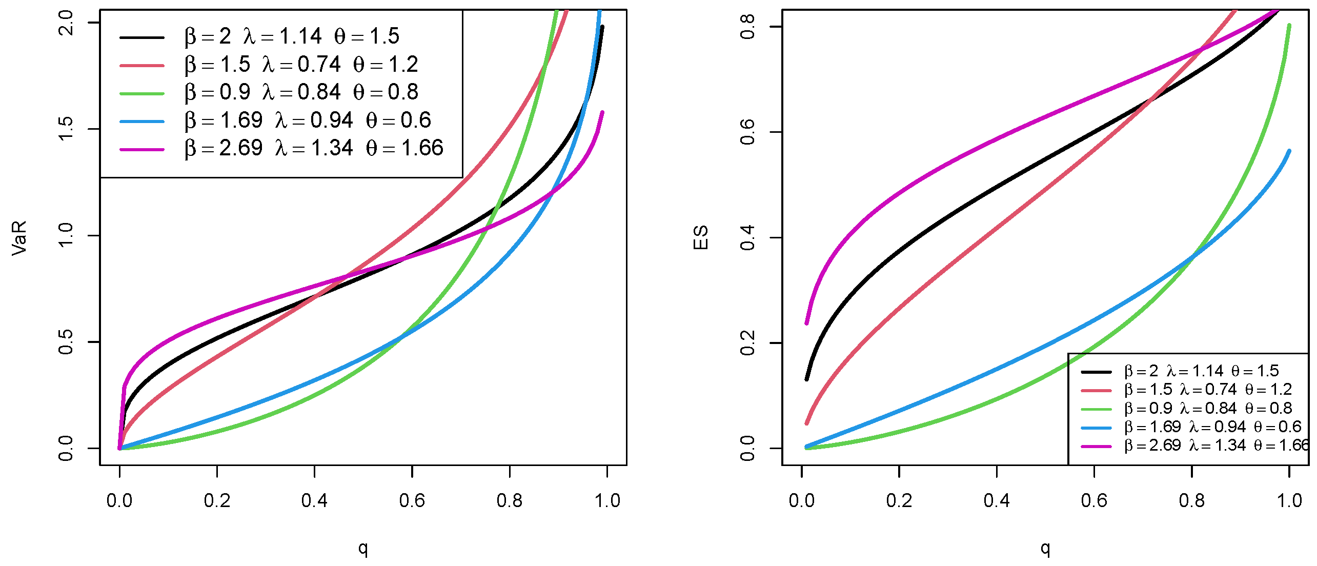
By substituting expressions (42) and (41) in (43), the T V P for the SEW model is obtained. A random sample of size 100 is selected, and the effects of the shape and scale parameters of the proposed models are analyzed under various risk measures. Multiple combinations of these parameters are considered to examine their impacts on the results: I = [ β = 2 , λ = 1.14 , θ = 1.5 ] , II = [ β = 1.5 , λ = 0.74 , θ = 1.2 ] , III = [ β = 0.9 , λ = 0.84 , θ = 0.8 ] , IV = [ β = 1.69 , λ = 0.94 , θ = 0.6 ] , and V = [ β = 2.69 , λ = 1.34 , θ = 1.66 ] . The changes in the curves of the Value at Risk (VaR) and expected shortfall (ES) are illustrated in Figure 3.

Numerical Illustration of VaR and ES

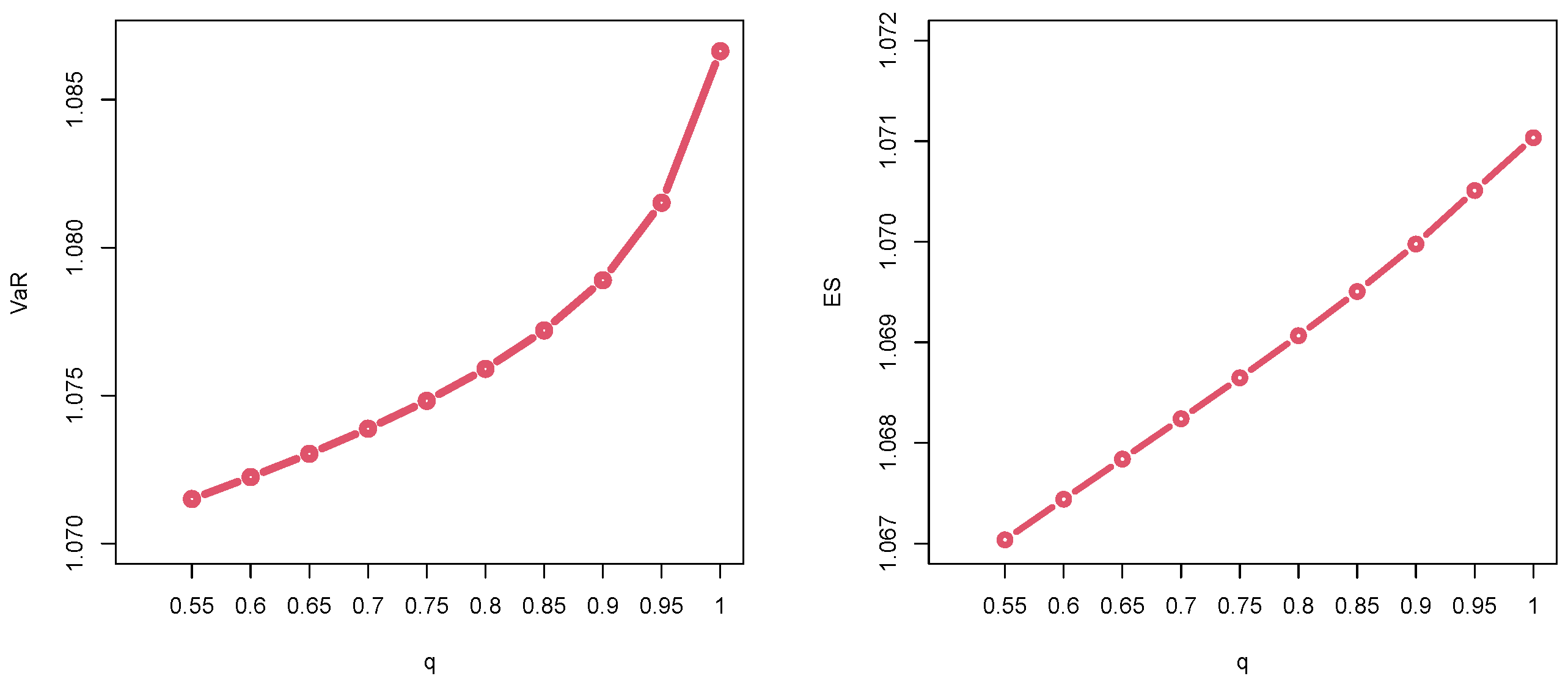
Here, we present the numerical and graphical representations of two important risk measures, VaR and ES, for the SEW distribution. It is noted that a model exhibiting higher values of these risk measures is considered to have a heavier tail. Table 14 provides the numerical values of VaR and ES for the SEW distribution, while the graphical illustration is shown in Figure 11. For a detailed explanation of VaR and ES, along with their implementation in R, the reader is referred to [65].
Figure 10 illustrates the behavior of VaR and ES of the SEW distribution for different parametric values, showing that both the ES and VaR values grow smoothly as the parameters change. Figure 11 is used to examine the trend of the real-life insurance claim data. The values in Table 14 display the estimated VaR and ES for the SEW distribution using the MLEs of the insurance claim data at various quantile levels. In Figure 11, it can be seen that both the ES and VaR values grow smoothly as the quantile q increases from 0.55 to 0.99, indicating the greater extent of financial risk in extreme tails. The ES values are also marginally lower than the respective VaR values, as expected from their theoretical definitions, as ES reflects the average loss in excess of the VaR. This upward trend confirms that the SEW distribution is a consistent and sound risk measure for tail behavior modeling in insurance claims.

8. Conclusions

This paper presents a new method consisting of a three-parameter flexible extension of the Weibull distribution, which is referred to as the SEW distribution. The paper investigates the mathematical properties of the SEW distribution with a comprehensive analysis of such properties and their effects on statistical modeling. To approximate the parameters of the novel model, eight estimation procedures are evaluated in relation to their efficiency. The reliability of these methods is appraised using prevalent simulation results, presenting a detailed study of their effectiveness and reliability. From the comparison, RSS is always better than SRS in estimating the SEW distribution’s parameters. RSS gives lower MSEs for a range of different parameter values and sample sizes. It is resistant to parameter inflation and more efficient for small and large parameter regimes. Thus, RSS is a superior and efficient estimator of parameters in the SEW model. Three real datasets are used to showcase the practical implementation of the SEW distribution, showing that it is significantly superior to several prominent competing models, including L1, L2, L3, L4, L5, L6, and L7. The results show the flexibility of the SEW distribution to accommodate a wide variety of data structures. Moreover, the article illustrates different characteristics of the SEW distribution and proves its applicability in various areas, such as reliability, medical, and finance analysis. Furthermore, the risk measure analysis of the third dataset, specifically focusing on ES and VaR, confirms the superiority of the SEW distribution in better capturing tail risk. This overall evidence establishes the real-world applicability of the SEW distribution in various fields. The suggested distribution presents new research opportunities, as its characteristic features can be utilized to study problems in a variety of fields. Future research can investigate further the real-world implications of the SEW distribution, resulting in improved models for application to statistics.

Author Contributions

Conceptualization, B.E.; methodology, B.E. and F.J.; software, Z.H. and F.J.; data curation, F.J.; writing—original draft, S.I.; writing—review and editing, S.I.; visualization, Z.H. and F.J. All authors have read and agreed to the published version of the manuscript.

Funding

This work was supported and funded by the Deanship of Scientific Research at Imam Mohammad ibn Saud Islamic University (IMSIU) (grant number IMSIU-DDRSP2601).

Data Availability Statement

The original contributions presented in this study are included in the article. Further inquiries can be directed to the corresponding author.

Conflicts of Interest

The authors declare no conflicts of interest.

References

  1. Meeker, W.Q.; Escobar, L.A.; Pascual, F.G. Statistical Methods for Reliability Data; John Wiley and Sons: Hoboken, NJ, USA, 2021. [Google Scholar]
  2. Gaidai, O.; Yakimov, V.; Wang, F.; Cao, Y. Gaidai multivariate reliability method for energy harvester operational safety, given manufacturing imperfections. Int. J. Precis. Eng. Manuf. 2024, 25, 1011–1025. [Google Scholar] [CrossRef]
  3. Embrechts, P.; Kluppelberg, C.; Mikosch, T. Modelling Extremal Events: For Insurance and Finance; Springer Science and Business Media: Berlin/Heidelberg, Germany, 2013; Volume 33. [Google Scholar]
  4. Alshanbari, H.M.; Ahmad, Z.; El-Bagoury, A.A.A.H.; Odhah, O.H.; Rao, G.S. A new modification of the Weibull distribution: Model, theory, and analyzing engineering data sets. Symmetry 2024, 16, 611. [Google Scholar] [CrossRef]
  5. Mudholkar, G.S.; Srivastava, D.K. Exponentiated Weibull family for analyzing bathtub failure-rate data. IEEE Trans. Reliab. 1993, 42, 299–302. [Google Scholar] [CrossRef]
  6. Famoye, F.; Lee, C.; Olumolade, O. The beta-Weibull distribution. J. Stat. Theory Appl. 2005, 4, 121–136. [Google Scholar]
  7. Keller, A.Z.; Kamath, A.R.R.; Perera, U.D. Reliability analysis of CNC machine tools. Reliab. Eng. 1982, 3, 449–473. [Google Scholar] [CrossRef]
  8. Lai, C.D.; Xie, M.; Murthy, D.N.P. A modified Weibull distribution. IEEE Trans. Reliab. 2003, 52, 33–37. [Google Scholar] [CrossRef]
  9. Shama, M.S.; Alharthi, A.S.; Almulhim, F.A.; Gemeay, A.M.; Meraou, M.A.; Mustafa, M.S.; Aljohani, H.M. Modified generalized Weibull distribution: Theory and applications. Sci. Rep. 2023, 13, 12828. [Google Scholar] [CrossRef] [PubMed]
  10. Alsulami, D.; Alghamdi, A.S. A New Extended Weibull Distribution: Estimation Methods and Applications in Engineering, Physics, and Medicine. Mathematics 2025, 13, 3262. [Google Scholar] [CrossRef]
  11. Al-Moisheer, A.S.; Sultan, K.S.; Radwan, H.M. A novel adaptable Weibull distribution and its applications. Axioms 2025, 14, 490. [Google Scholar] [CrossRef]
  12. Zanboori, A.; Zanboori, E.; Parvin, H.; Mahmoudi, M. A flexible Weibull geometric distribution with characterizations and its parameter estimation. Sci. Rep. 2025, 15, 26372. [Google Scholar] [CrossRef]
  13. Li, X.; Gong, Q.; Chen, T. Statistical inference and applications of a new transforming Weibull distribution. Sci. Rep. 2025, 15, 28970. [Google Scholar] [CrossRef]
  14. Begum, S.; Karim, M.R. The modified kies-weibull distribution: A flexible model for survival analysis. Int. J. Data Sci. Anal. 2025, 11, 6–16. [Google Scholar] [CrossRef]
  15. Chaturvedi, P.; Pokhriyal, H. Parameter estimation of the four-parameter Harris extended Weibull distribution with applications to real-life data. arXiv 2025, arXiv:2509.26162. [Google Scholar]
  16. Ahmed, Z.A.; Mohammed, A.T.; Enver, A. New Lifetime Alpha Power Rayleigh Weibull Distribution: Structure and Properties. Ibn AL-Haitham J. Pure Appl. Sci. 2025, 38, 352–362. [Google Scholar] [CrossRef]
  17. Gbemiga, A.S.; Afolabi, J.M. Development of Gompertz Generalised Weibull Distribution: Properties and Applications. Frontline Prof. J. 2025, 2, 24–34. [Google Scholar]
  18. Abdelkawy, M.A.; Alghamdi, S.M.; Elbatal, I.; Hashem, A.F.; Shawki, A.W.; Elgarhy, M. Statistical analysis of disability: Utilizing the new extended Rayleigh inverted Weibull model. Alex. Eng. J. 2025, 129, 779–792. [Google Scholar] [CrossRef]
  19. El-Saeed, A.R.; Elbatal, I.; Almetwally, E.M.; Elgarhy, M. Bayesian and Non-Bayesian Inference for the Trigonometric Extended Rayleigh-Weibull Model Under Progressively Censored Data. IEEE Access 2025, 13, 117043–117064. [Google Scholar] [CrossRef]
  20. Elgarhy, M.; Abdalla, G.S.S.; Obulezi, O.J.; Almetwally, E.M. A tangent DUS family of distributions with applications to the Weibull model. Sci. Afr. 2025, 29, e02843. [Google Scholar] [CrossRef]
  21. Bashiru, S.O.; Abdalla, G.S.S.; Ragab, I.E.; Elbatal, I.; Gemeay, A.M.; Elgarhy, M. Type II Half-Logistic Rayleigh Weibull distribution with statistical inference and applications. Sci. Afr. 2025, 30, e02927. [Google Scholar] [CrossRef]
  22. Nadir, S.; Ali, E.I.; Semary, H.E.; Aslam, M.; Obulezi, O.J.; Nasiru, S.; Elgarhy, M. Burr III Scaled Inverse Odds Ratio-Weibull Distribution for Modeling Asymmetric Medical and Engineering Data. Eng. Rep. 2025, 7, e70482. [Google Scholar] [CrossRef]
  23. Ado Osi, A.; Metwally, D.S.; Semary, H.E.; Ahmad Sabo, S.; Zakariyya Musa, I.; Hussein Mohamud, M.; Elgarhy, M. The New Heavy-Tailed Cosine-Weibull Distribution: Properties, Simulation, Applications, and Regression Modeling. Eng. Rep. 2025, 7, e70477. [Google Scholar] [CrossRef]
  24. Alotaibi, N.; Elbatal, I.; Almetwally, E.M.; Alyami, S.A.; Al-Moisheer, A.S.; Elgarhy, M. Bivariate Step-Stress Accelerated Life Tests for the Kavya-Manoharan Exponentiated Weibull Model under Progressive Censoring with Applications. Symmetry 2022, 14, 1791. [Google Scholar] [CrossRef]
  25. Alotaibi, N.; Elbatal, I.; Almetwally, E.M.; Alyami, S.A.; Al-Moisheer, A.S.; Elgarhy, M. Truncated Cauchy Power Weibull-G Class of Distributions: Bayesian and Non-Bayesian Inference Modelling for COVID-19 and Carbon Fiber Data. Mathematics 2022, 10, 1565. [Google Scholar] [CrossRef]
  26. Alyami, S.A.; Elbatal, I.; Alotaibi, N.; Almetwally, E.M.; Okasha, H.M.; Elgarhy, M. Topp-Leone Modified Weibull Model: Theory and Applications to Medical and Engineering Data. Appl. Sci. 2022, 12, 10431. [Google Scholar] [CrossRef]
  27. Almarashi, A.M.; Jamal, F.; Chesneau, C.; Elgarhy, M. The Exponentiated Truncated Inverse Weibull-Generated Family of Distributions with Applications. Symmetry 2020, 12, 650. [Google Scholar] [CrossRef]
  28. Aldahlan, M.A.; Jamal, F.; Chesneau, C.; Elbatal, I.; Elgarhy, M. Exponentiated power generalized Weibull power series family of distributions: Properties, estimation and applications. PLoS ONE 2020, 20, e0230004. [Google Scholar] [CrossRef]
  29. Alkarni, S.H.; Afify, A.Z.; Elbatal, I.; Elgarhy, M. The extended inverse Weibull distribution: Properties and applications. Complexity 2020, 2020, 3297693. [Google Scholar] [CrossRef]
  30. Hassan, A.S.; Elgarhy, M. Exponentiated Weibull-Weibull Distribution: Statistical Properties and Applications. Gazi J. Sci. 2019, 32, 616–635. [Google Scholar]
  31. Awadalla, M.; Murugesan, M. Bayesian Fractional Weibull Regression for Reliability Prognostics and Predictive Maintenance. Mathematics 2026, 14, 169. [Google Scholar] [CrossRef]
  32. Bourguignon, M.; Silva, R.B.; Cordeiro, G.M. The Weibull-G family of probability distributions. J. Data Sci. 2014, 12, 53–68. [Google Scholar] [CrossRef]
  33. Alzaatreh, A.; Famoye, F.; Lee, C. A new method for generating families of continuous distributions. Metron 2013, 71, 63–79. [Google Scholar] [CrossRef]
  34. Tahir, M.H.; Cordeiro, G.M.; Alizadeh, M.; Mansoor, M.; Zubair, M.; Hamedani, G.G. The odd generalized exponential family of distributions with applications. J. Stat. Distrib. Appl. 2015, 2, 1. [Google Scholar] [CrossRef]
  35. Kakwani, N.C.; Podder, N. Efficient estimation of the Lorenz curve and associated inequality measures from grouped observations. In Modeling Income Distributions and Lorenz Curves; Springer: New York, NY, USA, 2008; pp. 57–70. [Google Scholar]
  36. Elgarhy, M. Garhy distribution with different estimation methods and applications to engineering and medical data. Rev. Int. Métodos Numéricos Para Cálculo Diseño Ing. 2026, 1, 61. [Google Scholar]
  37. Pham-Gia, T.; Hung, T. The mean and median absolute deviations. Math. Comput. Model. 2001, 34, 921–936. [Google Scholar] [CrossRef]
  38. Al-Saleh, M.F.; Al-Hadhrami, S.A. Estimation of the mean of the exponential distribution using moving extremes ranked set sampling. Stat. Pap. 2003, 44, 367–382. [Google Scholar] [CrossRef]
  39. Chen, Z.; Bai, Z.; Sinha, B.K. Ranked Set Sampling: Theory and Applications; Springer: Berlin/Heidelberg, Germany, 2004; Volume 176. [Google Scholar]
  40. Imran, M.; Al-Essa, L.A.; Tahir, M.H.; Chesneau, C.; Shakoor, S.; Jamal, F. An extended exponential model: Estimation using ranked set sampling with applications. J. Radiat. Res. Appl. Sci. 2023, 16, 100642. [Google Scholar] [CrossRef]
  41. Bantan, R.; Elsehetry, M.; Hassan, A.S.; Elgarhy, M.; Sharma, D.; Chesneau, C.; Jamal, F. A two-parameter model: Properties and estimation under ranked sampling. Mathematics 2021, 9, 1214. [Google Scholar] [CrossRef]
  42. Metwally, D.S.; Hassan, A.S.; Almetwally, E.M.; Sapkota, L.P.; Gemeay, A.M.; Elgarhy, M. Different estimation methods for the unit Xgamma distribution using ranked set sampling. Eng. Rep. 2025, 7, e70157. [Google Scholar] [CrossRef]
  43. Alyami, S.A.; Hassan, A.S.; Elbatal, I.; Alotaibi, N.; Gemeay, A.M.; Elgarhy, M. Estimation methods based on ranked set sampling for the arctan uniform distribution with application. AIMS Math. 2024, 9, 10304–10332. [Google Scholar] [CrossRef]
  44. Alotaibi, N.; Elbatal, I.; Shrahili, M.; Al-Moisheer, A.S.; Elgarhy, M.; Almetwally, E.M. Statistical inference for the Kavya-Manoharan Kumaraswamy model under ranked set sampling with applications. Symmetry 2023, 15, 587. [Google Scholar] [CrossRef]
  45. Alotaibi, N.; Al-Moisheer, A.S.; Elbatal, I.; Shrahili, M.; Elgarhy, M.; Almetwally, E.M. Half Logistic Inverted Nadarajah-Haghighi distribution under ranked set sampling with applications. Mathematics 2023, 11, 1693. [Google Scholar] [CrossRef]
  46. Alsadat, N.; Hassan, A.S.; Elgarhy, M.; Chesneau, C.; Mohamed, R.E. An efficient stress-strength reliability estimate of the unit Gompertz distribution using ranked set sampling. Symmetry 2023, 15, 1121. [Google Scholar] [CrossRef]
  47. Yang, L. An evidence-based likelihood approach for the reliability of a complex system with overlapped failure data. Comput. Ind. Eng. 2025, 201, 110893. [Google Scholar] [CrossRef]
  48. David, H.A.; Nagaraja, H.N. Order Statistics; John Wiley and Sons: Hoboken, NJ, USA, 2004. [Google Scholar]
  49. Arnold, B.C.; Balakrishnan, N.; Nagaraja, H.N. A First Course in Order Statistics; Society for Industrial and Applied Mathematics: Philadelphia, PA, USA, 2008. [Google Scholar]
  50. Balakrishnan, N.; Rao, C.R. Handbook of Statistics Volume 16: Order Statistics: Theory and Methods; Elsevier: Amsterdam, The Netherlands, 1998. [Google Scholar]
  51. Shaked, M.; Shanthikumar, J.G. Stochastic Orders; Springer: New York, NY, USA, 2007. [Google Scholar]
  52. Chandler, K. The distribution and frequency of record values. J. R. Stat. Soc. Ser. B (Methodol.) 1952, 14, 220–228. [Google Scholar] [CrossRef]
  53. Lawless, J.F. Statistical Models and Methods for Lifetime Data; John Wiley and Sons: Hoboken, NJ, USA, 2011. [Google Scholar]
  54. Klein, J.P.; Moeschberger, M.L. Survival Analysis: Techniques for Censored and Truncated Data; Springer: Berlin/Heidelberg, Germany, 2006. [Google Scholar]
  55. Alanzi, A.R.; Rafique, M.Q.; Tahir, M.H.; Sami, W.; Jamal, F. A new modified kumaraswamy distribution: Actuarial measures and applications. J. Math. 2022, 2022, 4288286. [Google Scholar] [CrossRef]
  56. Xie, M.; Lai, C.D. Reliability analysis using an additive Weibull model with bathtub-shaped failure rate function. Reliab. Eng. Syst. Saf. 1996, 52, 87–93. [Google Scholar] [CrossRef]
  57. Marshall, A.W.; Olkin, I. A new method for adding a parameter to a family of distributions with application to the exponential and Weibull families. Biometrika 1997, 84, 641–652. [Google Scholar] [CrossRef]
  58. Keller, A.Z.; Kamath, A.R. Reliability analysis of the inverse Weibull distribution. Microelectron. Reliab. 1982, 22, 255–262. [Google Scholar]
  59. Burr, I.W. Cumulative frequency functions. Ann. Math. Stat. 1942, 13, 215–232. [Google Scholar] [CrossRef]
  60. Alzaghal, A.; Famoye, F.; Lee, C. The log-transformed generalized family of distributions with applications. J. Stat. Distrib. Appl. 2013, 1, 1–21. [Google Scholar]
  61. Yang, L.; Wang, J.; Xie, M. Graph-based reliability evaluation of a reconfigurable multi-stage system using sequential unconnected path sets. Reliab. Eng. Syst. Saf. 2025, 261, 111093. [Google Scholar] [CrossRef]
  62. Embrechts, P. Quantitative risk management. In International Encyclopedia of Statistical Science; Springer: Berlin/Heidelberg, Germany, 2025; pp. 2050–2054. [Google Scholar]
  63. Klugman, S.A.; Panjer, H.H.; Willmot, G.E. Loss Models: From Data to Decisions; John Wiley and Sons: Hoboken, NJ, USA, 2012; Volume 715. [Google Scholar]
  64. Artzner, P.; Delbaen, F.; Eber, J.M.; Heath, D. Coherent measures of risk. Math. Financ. 1999, 9, 203–228. [Google Scholar] [CrossRef]
  65. Chan, N.H.; Chen, H.; Wang, J. Financial Risk Management: Applications in Market, Credit, Asset and Liability Management and Firmwide Risk; Wiley: Hoboken, NJ, USA, 2020. [Google Scholar]
Figure 1. PDF plots of the SEW distribution.
Symmetry 18 00659 g001
Figure 2. HRF plots of the SEW distribution.
Symmetry 18 00659 g002
Figure 3. MSE of the SEW distribution under different sample sizes ( n = 30 , n = 50 , and n = 100 ) for SRS and RSS methods.
Symmetry 18 00659 g003
Figure 4. Dataset 1 visualized through a T T T plot, boxplot, kernel density plot, and violin plot.
Symmetry 18 00659 g004
Figure 5. Dataset 2 visualized through a T T T plot, boxplot, kernel density plot, and violin plot.
Symmetry 18 00659 g005
Figure 6. Dataset 3 visualized through a T T T plot, boxplot, kernel density plot, and violin plot.
Symmetry 18 00659 g006
Figure 7. Visualization of the PDFs and CDFs for comparison with the SEW distribution based on Dataset 1.
Symmetry 18 00659 g007
Figure 8. Visualization of the PDFs and CDFs for comparison with the SEW distribution based on Dataset 2.
Symmetry 18 00659 g008
Figure 9. Visualization of the PDFs and CDFs for comparison with the SEW distribution based on Dataset 3.
Symmetry 18 00659 g009
Figure 10. Plots of VaR and ES of SEW distribution for some parametric values.
Symmetry 18 00659 g010
Figure 11. Plots of VaR and ES of SEW distribution based on MLEs of insurance claim data.
Symmetry 18 00659 g011
Table 1. Special cases of the proposed SEW distribution.
CaseParameter SettingResulting FormInterpretation
1 θ = 1 F ( x ) = e e 1 1 exp ( 1 exp ( λ x β ) ) Simplified transformed Weibull model
2 β = 1 F ( x ) = e e 1 1 exp ( 1 exp ( λ x ) ) θ Exponential-based extension
3 θ = 1 , β = 1 F ( x ) = e e 1 1 exp ( 1 exp ( λ x ) ) Transformed exponential model
Table 2. Numerical results for moments, SD, Sk, and Ku of SEW.
β λ θ μ 1 μ 2 μ 3 μ 4 SDSkKu
2.01.11.10.7604350.7479260.8842701.2045090.4119030.8225393.703541
2.51.11.10.7843210.7341710.7844730.9310370.3449820.5348503.138593
2.71.11.10.7931640.7346260.7654140.8764050.3248340.4478473.020946
3.01.11.10.8054660.7383000.7479260.8218000.2992070.3372182.907147
2.71.51.10.7070900.5838340.5422900.5535430.2895830.4478473.020946
2.72.01.10.6356250.4717830.3939220.3614570.2603160.4478473.020946
2.02.01.10.5639540.4113590.3606860.3643640.3054760.8225393.703541
2.02.51.10.5044160.3290880.2580860.2331930.2732260.8225393.703541
2.01.11.30.8221480.8420061.0175511.4027990.4075260.7714993.649624
2.01.11.50.8749550.9277241.1436211.5946530.4027140.7365653.623232
2.01.12.00.9800491.1132671.4315672.0481920.3908590.6877113.609530
2.71.11.30.8444180.8124130.8669411.0078970.3152310.4183453.045584
2.71.11.50.8872910.8813010.9603781.1321420.3066190.4013043.073014
2.71.11.70.9239190.9429921.0468521.2498390.2989410.3919203.099919
4.52.11.70.8153010.6908580.6059170.5482270.1616860.0073522.947706
4.82.11.70.82480.703930.6194790.5605620.153737−0.0306362.960829
5.22.11.70.8360550.7198080.6363860.5764390.144289−0.0750372.982774
5.52.11.70.8435980.7306840.6482310.587860.137937−0.1044553.001271
Table 3. Simulation results for λ = 2 , β = 1.5 , θ = 1.3 . Superscripts denote ranking of estimators based on performance (1 = best, higher numbers indicate lower performance).
n MLEOLSEWLSEMPSECVMEADERADE
30AB λ ^ 0.3142 ( 2 ) 0.4536 ( 6 ) 0.3796 ( 4 ) 0.1255 ( 1 ) 0.7370 ( 7 ) 0.3560 ( 3 ) 0.3819 ( 5 )
β ^ 0.8142 ( 3 ) 0.9536 ( 6 ) 0.8796 ( 5 ) 0.6255 ( 2 ) 1.2370 ( 7 ) 0.8560 ( 4 ) 0.1181 ( 1 )
θ ^ 1.0142 ( 3 ) 1.1536 ( 6 ) 1.0796 ( 5 ) 0.8255 ( 2 ) 1.4370 ( 7 ) 1.0560 ( 4 ) 0.3181 ( 1 )
MSE λ ^ 2.5586 ( 4 ) 3.2062 ( 6 ) 2.7632 ( 5 ) 1.8191 ( 3 ) 7.0543 ( 7 ) 1.5961 ( 2 ) 0.1516 ( 1 )
β ^ 3.1228 ( 4 ) 3.9098 ( 6 ) 3.3928 ( 5 ) 2.1946 ( 2 ) 8.0413 ( 7 ) 2.2020 ( 3 ) 0.0197 ( 1 )
θ ^ 3.4885 ( 4 ) 4.3313 ( 6 ) 3.7847 ( 5 ) 2.4848 ( 2 ) 8.5761 ( 7 ) 2.5844 ( 3 ) 0.1070 ( 1 )
MRE λ ^ 0.5344 ( 4 ) 0.5958 ( 6 ) 0.5378 ( 5 ) 0.4648 ( 2 ) 0.6829 ( 7 ) 0.4828 ( 3 ) 0.1910 ( 1 )
β ^ 0.8015 ( 4 ) 0.8903 ( 6 ) 0.8044 ( 5 ) 0.6657 ( 2 ) 1.0399 ( 7 ) 0.7523 ( 3 ) 0.0787 ( 1 )
θ ^ 0.9999 ( 4 ) 1.1031 ( 6 ) 1.0077 ( 5 ) 0.8303 ( 2 ) 1.2855 ( 7 ) 0.9552 ( 3 ) 0.2447 ( 1 )
Rank _32544418632813
50AB λ ^ 0.1267 ( 2 ) 0.1739 ( 4 ) 0.1572 ( 3 ) 0.0111 ( 1 ) 0.2606 ( 6 ) 0.1880 ( 5 ) 0.3950 ( 7 )
β ^ 0.6267 ( 3 ) 0.6739 ( 5 ) 0.6572 ( 4 ) 0.5111 ( 2 ) 0.7606 ( 7 ) 0.6880 ( 6 ) 0.1050 ( 1 )
θ ^ 0.8267 ( 3 ) 0.8739 ( 5 ) 0.8572 ( 4 ) 0.7111 ( 2 ) 0.9606 ( 7 ) 0.8880 ( 6 ) 0.3050 ( 1 )
MSE λ ^ 0.9453 ( 5 ) 1.0263 ( 6 ) 0.9004 ( 4 ) 0.8069 ( 2 ) 1.0753 ( 7 ) 0.8477 ( 3 ) 0.1607 ( 1 )
β ^ 1.3220 ( 5 ) 1.4502 ( 6 ) 1.3076 ( 4 ) 1.0680 ( 2 ) 1.5859 ( 7 ) 1.2857 ( 3 ) 0.0157 ( 1 )
θ ^ 1.6126 ( 5 ) 1.7597 ( 6 ) 1.6105 ( 4 ) 1.3124 ( 2 ) 1.9302 ( 7 ) 1.6009 ( 3 ) 0.0977 ( 1 )
MRE λ ^ 0.3533 ( 4 ) 0.4038 ( 6 ) 0.3679 ( 5 ) 0.3298 ( 2 ) 0.4125 ( 7 ) 0.3454 ( 3 ) 0.1975 ( 1 )
β ^ 0.5719 ( 3 ) 0.6282 ( 6 ) 0.5791 ( 5 ) 0.4958 ( 2 ) 0.6660 ( 7 ) 0.5721 ( 4 ) 0.0700 ( 1 )
θ ^ 0.7503 ( 3 ) 0.8084 ( 6 ) 0.7578 ( 4 ) 0.6533 ( 2 ) 0.8586 ( 7 ) 0.7601 ( 5 ) 0.2346 ( 1 )
Rank _33503717623815
100AB λ ^ 0.0862 ( 2 ) 0.1420 ( 5 ) 0.1163 ( 3 ) 0.0264 ( 1 ) 0.1860 ( 6 ) 0.1339 ( 4 ) 0.4200 ( 7 )
β ^ 0.5862 ( 3 ) 0.6420 ( 6 ) 0.6163 ( 4 ) 0.5264 ( 2 ) 0.6860 ( 7 ) 0.6339 ( 5 ) 0.0800 ( 1 )
θ ^ 0.7862 ( 3 ) 0.8420 ( 6 ) 0.8163 ( 4 ) 0.7264 ( 2 ) 0.8860 ( 7 ) 0.8339 ( 5 ) 0.2800 ( 1 )
MSE λ ^ 0.3222 ( 3 ) 0.5569 ( 6 ) 0.4185 ( 5 ) 0.2874 ( 2 ) 0.5740 ( 7 ) 0.3824 ( 4 ) 0.1786 ( 1 )
β ^ 0.6585 ( 3 ) 0.9489 ( 6 ) 0.7849 ( 5 ) 0.5638 ( 2 ) 1.0100 ( 7 ) 0.7663 ( 4 ) 0.0086 ( 1 )
θ ^ 0.9329 ( 3 ) 1.2457 ( 6 ) 1.0714 ( 5 ) 0.8143 ( 2 ) 1.3244 ( 7 ) 1.0598 ( 4 ) 0.0806 ( 1 )
MRE λ ^ 0.2202 ( 3 ) 0.2860 ( 6 ) 0.2483 ( 5 ) 0.2083 ( 1 ) 0.2895 ( 7 ) 0.2384 ( 4 ) 0.2100 ( 2 )
β ^ 0.4319 ( 3 ) 0.5064 ( 6 ) 0.4618 ( 5 ) 0.3927 ( 2 ) 0.5273 ( 7 ) 0.4613 ( 4 ) 0.0534 ( 1 )
θ ^ 0.6217 ( 3 ) 0.6928 ( 6 ) 0.6512 ( 4 ) 0.5733 ( 2 ) 0.7211 ( 7 ) 0.6558 ( 5 ) 0.2154 ( 1 )
Rank _26534016623916
150AB λ ^ 0.0726 ( 2 ) 0.1021 ( 5 ) 0.0782 ( 3 ) 0.0346 ( 1 ) 0.1294 ( 6 ) 0.0937 ( 4 ) 0.4217 ( 7 )
β ^ 0.5726 ( 3 ) 0.6021 ( 6 ) 0.5782 ( 4 ) 0.5346 ( 2 ) 0.6294 ( 7 ) 0.5937 ( 5 ) 0.0783 ( 1 )
θ ^ 0.7726 ( 3 ) 0.8021 ( 6 ) 0.7782 ( 4 ) 0.7346 ( 2 ) 0.8294 ( 7 ) 0.7937 ( 5 ) 0.2783 ( 1 )
MSE λ ^ 0.2014 ( 3 ) 0.3550 ( 6 ) 0.2513 ( 5 ) 0.1834 ( 2 ) 0.3593 ( 7 ) 0.2408 ( 4 ) 0.1795 ( 1 )
β ^ 0.5239 ( 3 ) 0.7070 ( 6 ) 0.5795 ( 4 ) 0.4680 ( 2 ) 0.7387 ( 7 ) 0.5845 ( 5 ) 0.0078 ( 1 )
θ ^ 0.7930 ( 3 ) 0.9879 ( 6 ) 0.8508 ( 4 ) 0.7218 ( 2 ) 1.0305 ( 7 ) 0.8619 ( 5 ) 0.0791 ( 1 )
MRE λ ^ 0.1751 ( 3 ) 0.2309 ( 5 ) 0.1960 ( 4 ) 0.1682 ( 1 ) 0.2323 ( 6 ) 0.1905 ( 2 ) 0.2109 ( 7 )
β ^ 0.3985 ( 3 ) 0.4467 ( 6 ) 0.4124 ( 4 ) 0.3733 ( 2 ) 0.4610 ( 7 ) 0.4173 ( 5 ) 0.0522 ( 1 )
θ ^ 0.5980 ( 3 ) 0.6400 ( 6 ) 0.6085 ( 4 ) 0.5687 ( 2 ) 0.6592 ( 7 ) 0.6178 ( 5 ) 0.2141 ( 1 )
Rank _26523616614021
200AB λ ^ 0.0518 ( 2 ) 0.0807 ( 5 ) 0.0602 ( 3 ) 0.0245 ( 1 ) 0.1029 ( 6 ) 0.0687 ( 4 ) 0.4280 ( 7 )
β ^ 0.5518 ( 3 ) 0.5807 ( 6 ) 0.5602 ( 4 ) 0.5245 ( 2 ) 0.6029 ( 7 ) 0.5687 ( 5 ) 0.0720 ( 1 )
θ ^ 0.7518 ( 3 ) 0.7807 ( 6 ) 0.7602 ( 4 ) 0.7245 ( 2 ) 0.8029 ( 7 ) 0.7687 ( 5 ) 0.2720 ( 1 )
MSE λ ^ 0.1335 ( 3 ) 0.2523 ( 6 ) 0.1692 ( 5 ) 0.1240 ( 1 ) 0.2610 ( 7 ) 0.1605 ( 4 ) 0.1839 ( 2 )
β ^ 0.4353 ( 3 ) 0.5830 ( 6 ) 0.4794 ( 5 ) 0.3985 ( 2 ) 0.6139 ( 7 ) 0.4792 ( 4 ) 0.0059 ( 1 )
θ ^ 0.6960 ( 3 ) 0.8552 ( 6 ) 0.7434 ( 4 ) 0.6482 ( 2 ) 0.8951 ( 7 ) 0.7466 ( 5 ) 0.0748 ( 1 )
MRE λ ^ 0.1446 ( 2 ) 0.1990 ( 5 ) 0.1627 ( 4 ) 0.1393 ( 1 ) 0.2010 ( 6 ) 0.1600 ( 3 ) 0.2140 ( 7 )
β ^ 0.3789 ( 3 ) 0.4132 ( 6 ) 0.3889 ( 4 ) 0.3607 ( 2 ) 0.4262 ( 7 ) 0.3928 ( 5 ) 0.0480 ( 1 )
θ ^ 0.5803 ( 3 ) 0.6132 ( 6 ) 0.5899 ( 4 ) 0.5592 ( 2 ) 0.6294 ( 7 ) 0.5955 ( 5 ) 0.2093 ( 1 )
Rank _25523714614023
300AB λ ^ 0.0180 ( 2 ) 0.0397 ( 5 ) 0.0208 ( 3 ) 0.0009 ( 1 ) 0.0532 ( 6 ) 0.0306 ( 4 ) 0.4256 ( 7 )
β ^ 0.5180 ( 3 ) 0.5397 ( 6 ) 0.5208 ( 4 ) 0.5009 ( 2 ) 0.5532 ( 7 ) 0.5306 ( 5 ) 0.0744 ( 1 )
θ ^ 0.7180 ( 3 ) 0.7397 ( 6 ) 0.7208 ( 4 ) 0.7009 ( 2 ) 0.7532 ( 7 ) 0.7306 ( 5 ) 0.2744 ( 1 )
MSE λ ^ 0.0840 ( 2 ) 0.1589 ( 5 ) 0.1038 ( 4 ) 0.0800 ( 1 ) 0.1596 ( 6 ) 0.1026 ( 3 ) 0.1817 ( 7 )
β ^ 0.3519 ( 3 ) 0.4486 ( 6 ) 0.3746 ( 4 ) 0.3309 ( 2 ) 0.4628 ( 7 ) 0.3832 ( 5 ) 0.0061 ( 1 )
θ ^ 0.5991 ( 3 ) 0.7045 ( 6 ) 0.6230 ( 4 ) 0.5712 ( 2 ) 0.7241 ( 7 ) 0.6354 ( 5 ) 0.0759 ( 1 )
MRE λ ^ 0.1137 ( 2 ) 0.1569 ( 5 ) 0.1243 ( 4 ) 0.1112 ( 1 ) 0.1575 ( 6 ) 0.1235 ( 3 ) 0.2128 ( 7 )
β ^ 0.3507 ( 3 ) 0.3777 ( 6 ) 0.3562 ( 4 ) 0.3394 ( 2 ) 0.3855 ( 7 ) 0.3619 ( 5 ) 0.0496 ( 1 )
θ ^ 0.5534 ( 3 ) 0.5754 ( 6 ) 0.5572 ( 4 ) 0.5402 ( 2 ) 0.5854 ( 7 ) 0.5642 ( 5 ) 0.2111 ( 1 )
Rank _24512715604027
Table 4. Simulation results for λ = 1.5 , β = 1.8 , θ = 1.6 . Superscripts denote ranking of estimators based on performance (1 = best, higher numbers indicate lower performance).
n MLEOLSEWLSEMPSECVMEADERADE
30AB λ ^ 0.2289 ( 3 ) 0.3201 ( 5 ) 0.3081 ( 4 ) 0.1763 ( 2 ) 0.4069 ( 7 ) 0.3300 ( 6 ) 0.0892 ( 1 )
β ^ 0.0712 ( 4 ) 0.0201 ( 2 ) 0.0081 ( 1 ) 0.1237 ( 6 ) 0.1069 ( 5 ) 0.0300 ( 3 ) 0.2108 ( 7 )
θ ^ 0.1289 ( 3 ) 0.2201 ( 5 ) 0.2081 ( 4 ) 0.0763 ( 2 ) 0.3069 ( 7 ) 0.2300 ( 6 ) 0.0108 ( 1 )
MSE λ ^ 1.9064 ( 6 ) 1.8739 ( 5 ) 1.8032 ( 4 ) 1.7210 ( 3 ) 2.0493 ( 7 ) 1.6591 ( 2 ) 0.0080 ( 1 )
β ^ 1.8591 ( 6 ) 1.7719 ( 5 ) 1.7083 ( 4 ) 1.7052 ( 3 ) 1.8952 ( 7 ) 1.5512 ( 2 ) 0.0445 ( 1 )
θ ^ 1.8706 ( 6 ) 1.8199 ( 5 ) 1.7516 ( 4 ) 1.6957 ( 3 ) 1.9779 ( 7 ) 1.6031 ( 2 ) 0.0002 ( 1 )
MRE λ ^ 0.6667 ( 4 ) 0.7372 ( 6 ) 0.6940 ( 5 ) 0.6176 ( 2 ) 0.7652 ( 7 ) 0.6487 ( 3 ) 0.0595 ( 1 )
β ^ 0.5747 ( 4 ) 0.6200 ( 6 ) 0.5906 ( 5 ) 0.5450 ( 2 ) 0.6359 ( 7 ) 0.5452 ( 3 ) 0.1171 ( 1 )
θ ^ 0.6272 ( 4 ) 0.6895 ( 6 ) 0.6519 ( 5 ) 0.5858 ( 2 ) 0.7137 ( 7 ) 0.6057 ( 3 ) 0.0067 ( 1 )
Rank _40453625613015
50AB λ ^ 0.1041 ( 3 ) 0.2060 ( 6 ) 0.1748 ( 4 ) 0.0682 ( 1 ) 0.2472 ( 7 ) 0.1800 ( 5 ) 0.0905 ( 2 )
β ^ 0.1959 ( 5 ) 0.0940 ( 2 ) 0.1252 ( 4 ) 0.2318 ( 7 ) 0.0528 ( 1 ) 0.1200 ( 3 ) 0.2095 ( 6 )
θ ^ 0.0041 ( 1 ) 0.1060 ( 6 ) 0.0748 ( 4 ) 0.0318 ( 3 ) 0.1472 ( 7 ) 0.0800 ( 5 ) 0.0095 ( 2 )
MSE λ ^ 0.9714 ( 4 ) 1.2352 ( 6 ) 1.0660 ( 5 ) 0.8656 ( 2 ) 1.2670 ( 7 ) 0.9196 ( 3 ) 0.0082 ( 1 )
β ^ 0.9990 ( 4 ) 1.2016 ( 6 ) 1.0512 ( 5 ) 0.9147 ( 3 ) 1.2087 ( 7 ) 0.9016 ( 2 ) 0.0439 ( 1 )
θ ^ 0.9606 ( 4 ) 1.2040 ( 6 ) 1.0411 ( 5 ) 0.8619 ( 2 ) 1.2276 ( 7 ) 0.8936 ( 3 ) 0.0001 ( 1 )
MRE λ ^ 0.4668 ( 3 ) 0.5816 ( 6 ) 0.5211 ( 5 ) 0.4728 ( 4 ) 0.5898 ( 7 ) 0.4402 ( 2 ) 0.0604 ( 1 )
β ^ 0.4210 ( 4 ) 0.5030 ( 6 ) 0.4582 ( 5 ) 0.4078 ( 2 ) 0.5033 ( 7 ) 0.4193 ( 3 ) 0.1164 ( 1 )
θ ^ 0.4430 ( 3 ) 0.5479 ( 6 ) 0.4936 ( 5 ) 0.4211 ( 2 ) 0.5526 ( 7 ) 0.4468 ( 4 ) 0.0059 ( 1 )
Rank _31504226573016
100AB λ ^ 0.0783 ( 2 ) 0.1659 ( 6 ) 0.1271 ( 4 ) 0.0618 ( 1 ) 0.1840 ( 7 ) 0.1371 ( 5 ) 0.0911 ( 3 )
β ^ 0.2217 ( 6 ) 0.1341 ( 2 ) 0.1729 ( 4 ) 0.2382 ( 7 ) 0.1161 ( 1 ) 0.1629 ( 3 ) 0.2089 ( 5 )
θ ^ 0.0217 ( 2 ) 0.0659 ( 6 ) 0.0271 ( 3 ) 0.0371 ( 4 ) 0.0839 ( 7 ) 0.0382 ( 5 ) 0.0089 ( 1 )
MSE λ ^ 0.3379 ( 3 ) 0.6958 ( 7 ) 0.4862 ( 5 ) 0.3152 ( 2 ) 0.6888 ( 6 ) 0.4332 ( 4 ) 0.0083 ( 1 )
β ^ 0.3809 ( 3 ) 0.6863 ( 7 ) 0.4999 ( 5 ) 0.3681 ( 2 ) 0.6684 ( 6 ) 0.4409 ( 4 ) 0.0437 ( 1 )
θ ^ 0.3323 ( 3 ) 0.6726 ( 7 ) 0.4707 ( 5 ) 0.3128 ( 2 ) 0.6620 ( 6 ) 0.4158 ( 4 ) 0.0001 ( 1 )
MRE λ ^ 0.2963 ( 3 ) 0.4198 ( 6 ) 0.3522 ( 5 ) 0.2847 ( 2 ) 0.4203 ( 7 ) 0.3321 ( 4 ) 0.0607 ( 1 )
β ^ 0.2783 ( 3 ) 0.3718 ( 7 ) 0.3176 ( 5 ) 0.2730 ( 2 ) 0.3682 ( 6 ) 0.2995 ( 4 ) 0.1161 ( 1 )
θ ^ 0.2809 ( 3 ) 0.3957 ( 7 ) 0.3330 ( 5 ) 0.2716 ( 2 ) 0.3942 ( 6 ) 0.3130 ( 4 ) 0.0059 ( 1 )
Rank _28554124523715
150AB λ ^ 0.0682 ( 2 ) 0.1119 ( 6 ) 0.0854 ( 3 ) 0.0614 ( 1 ) 0.1297 ( 7 ) 0.0965 ( 5 ) 0.0911 ( 4 )
β ^ 0.2318 ( 6 ) 0.1881 ( 2 ) 0.2146 ( 5 ) 0.2386 ( 7 ) 0.1703 ( 1 ) 0.2035 ( 4 ) 0.2089 ( 3 )
θ ^ 0.0318 ( 6 ) 0.0119 ( 3 ) 0.0146 ( 4 ) 0.0386 ( 7 ) 0.0297 ( 5 ) 0.0035 ( 1 ) 0.0089 ( 2 )
MSE λ ^ 0.2072 ( 3 ) 0.4114 ( 6 ) 0.2819 ( 5 ) 0.1953 ( 2 ) 0.4301 ( 7 ) 0.2645 ( 4 ) 0.0083 ( 1 )
β ^ 0.2563 ( 3 ) 0.4343 ( 6 ) 0.3206 ( 5 ) 0.2485 ( 2 ) 0.4423 ( 7 ) 0.2967 ( 4 ) 0.0437 ( 1 )
θ ^ 0.2036 ( 3 ) 0.3991 ( 6 ) 0.2748 ( 5 ) 0.1930 ( 2 ) 0.4142 ( 7 ) 0.2552 ( 4 ) 0.0001 ( 1 )
MRE λ ^ 0.2362 ( 3 ) 0.3331 ( 6 ) 0.2741 ( 5 ) 0.2292 ( 2 ) 0.3370 ( 7 ) 0.2624 ( 4 ) 0.0607 ( 1 )
β ^ 0.2324 ( 3 ) 0.2958 ( 6 ) 0.2551 ( 5 ) 0.2298 ( 2 ) 0.2958 ( 7 ) 0.2448 ( 4 ) 0.1161 ( 1 )
θ ^ 0.2239 ( 3 ) 0.3114 ( 6 ) 0.2570 ( 5 ) 0.2185 ( 2 ) 0.3140 ( 7 ) 0.2460 ( 4 ) 0.0057 ( 1 )
Rank _32474227553415
200AB λ ^ 0.0482 ( 2 ) 0.0945 ( 6 ) 0.0656 ( 3 ) 0.0454 ( 1 ) 0.1052 ( 7 ) 0.0703 ( 4 ) 0.0911 ( 5 )
β ^ 0.2518 ( 6 ) 0.2056 ( 2 ) 0.2344 ( 5 ) 0.2546 ( 7 ) 0.1948 ( 1 ) 0.2297 ( 4 ) 0.2089 ( 3 )
θ ^ 0.0518 ( 6 ) 0.0056 ( 2 ) 0.0344 ( 5 ) 0.0546 ( 7 ) 0.0052 ( 1 ) 0.0297 ( 4 ) 0.0089 ( 3 )
MSE λ ^ 0.1344 ( 3 ) 0.3161 ( 6 ) 0.1888 ( 5 ) 0.1281 ( 2 ) 0.3188 ( 7 ) 0.1760 ( 4 ) 0.0083 ( 1 )
β ^ 0.1954 ( 3 ) 0.3494 ( 6 ) 0.2395 ( 5 ) 0.1909 ( 2 ) 0.3457 ( 7 ) 0.2238 ( 4 ) 0.0437 ( 1 )
θ ^ 0.1347 ( 3 ) 0.3072 ( 6 ) 0.1857 ( 5 ) 0.1291 ( 2 ) 0.3078 ( 7 ) 0.1719 ( 4 ) 0.0001 ( 1 )
MRE λ ^ 0.1922 ( 3 ) 0.2941 ( 6 ) 0.2264 ( 5 ) 0.1878 ( 2 ) 0.2954 ( 7 ) 0.2199 ( 4 ) 0.0607 ( 1 )
β ^ 0.2008 ( 3 ) 0.2741 ( 7 ) 0.2232 ( 5 ) 0.1991 ( 2 ) 0.2728 ( 6 ) 0.2165 ( 4 ) 0.1161 ( 1 )
θ ^ 0.1809 ( 3 ) 0.2797 ( 6 ) 0.2149 ( 5 ) 0.1777 ( 2 ) 0.2800 ( 7 ) 0.2074 ( 4 ) 0.0055 ( 1 )
Rank _32474327503617
300AB λ ^ 0.0164 ( 1 ) 0.0475 ( 5 ) 0.0237 ( 3 ) 0.0165 ( 2 ) 0.0553 ( 6 ) 0.0326 ( 4 ) 0.0911 ( 7 )
β ^ 0.2836 ( 7 ) 0.2525 ( 3 ) 0.2764 ( 5 ) 0.2835 ( 6 ) 0.2447 ( 2 ) 0.2674 ( 4 ) 0.2089 ( 1 )
θ ^ 0.0836 ( 7 ) 0.0525 ( 3 ) 0.0764 ( 5 ) 0.0835 ( 6 ) 0.0447 ( 2 ) 0.0674 ( 4 ) 0.0089 ( 1 )
MSE λ ^ 0.0865 ( 3 ) 0.1962 ( 6 ) 0.1175 ( 5 ) 0.0834 ( 2 ) 0.1983 ( 7 ) 0.1157 ( 4 ) 0.0083 ( 1 )
β ^ 0.1667 ( 3 ) 0.2576 ( 7 ) 0.1933 ( 5 ) 0.1635 ( 2 ) 0.2551 ( 6 ) 0.1861 ( 4 ) 0.0437 ( 1 )
θ ^ 0.0932 ( 3 ) 0.1967 ( 6 ) 0.1227 ( 5 ) 0.0901 ( 2 ) 0.1972 ( 7 ) 0.1191 ( 4 ) 0.0001 ( 1 )
MRE λ ^ 0.1530 ( 3 ) 0.2329 ( 6 ) 0.1781 ( 5 ) 0.1503 ( 2 ) 0.2339 ( 7 ) 0.1768 ( 4 ) 0.0607 ( 1 )
β ^ 0.1904 ( 3 ) 0.2320 ( 7 ) 0.2022 ( 5 ) 0.1893 ( 2 ) 0.2305 ( 6 ) 0.1984 ( 4 ) 0.1161 ( 1 )
θ ^ 0.1522 ( 3 ) 0.2218 ( 7 ) 0.1714 ( 5 ) 0.1497 ( 2 ) 0.2217 ( 6 ) 0.1693 ( 4 ) 0.0055 ( 1 )
Rank _33504326493615
Table 5. Simulation results for λ = 1.2 , β = 2 , θ = 2.3 . Superscripts denote ranking of estimators based on performance (1 = best, higher numbers indicate lower performance).
n MLEOLSEWLSEMPSECVMEADERADE
30AB λ ^ 0.3176 ( 2 ) 0.3320 ( 4 ) 0.3266 ( 3 ) 0.3162 ( 1 ) 0.3619 ( 6 ) 0.3534 ( 5 ) 0.3650 ( 7 )
β ^ 0.4825 ( 6 ) 0.4680 ( 4 ) 0.4734 ( 5 ) 0.4838 ( 7 ) 0.4381 ( 2 ) 0.4466 ( 3 ) 0.4350 ( 1 )
θ ^ 0.7825 ( 6 ) 0.7680 ( 4 ) 0.7734 ( 5 ) 0.7838 ( 7 ) 0.7381 ( 2 ) 0.7466 ( 3 ) 0.7350 ( 1 )
MSE λ ^ 2.1155 ( 7 ) 1.7144 ( 4 ) 1.6742 ( 2 ) 2.0776 ( 6 ) 1.7560 ( 5 ) 1.6764 ( 3 ) 0.1340 ( 1 )
β ^ 2.2474 ( 7 ) 1.8232 ( 5 ) 1.7916 ( 3 ) 2.2117 ( 6 ) 1.8169 ( 4 ) 1.7510 ( 2 ) 0.1901 ( 1 )
θ ^ 2.6269 ( 7 ) 2.1940 ( 5 ) 2.1656 ( 3 ) 2.5920 ( 6 ) 2.1697 ( 4 ) 2.1089 ( 2 ) 0.5411 ( 1 )
MRE λ ^ 0.8435 ( 4 ) 0.8927 ( 6 ) 0.8466 ( 5 ) 0.8179 ( 3 ) 0.9067 ( 7 ) 0.8096 ( 2 ) 0.3041 ( 1 )
β ^ 0.6150 ( 7 ) 0.6032 ( 5 ) 0.5908 ( 3 ) 0.6058 ( 6 ) 0.6025 ( 4 ) 0.5679 ( 2 ) 0.2175 ( 1 )
θ ^ 0.6042 ( 7 ) 0.5744 ( 5 ) 0.5704 ( 4 ) 0.5982 ( 6 ) 0.5702 ( 3 ) 0.5556 ( 2 ) 0.3196 ( 1 )
Rank _53423348372415
50MRE λ ^ 0.1314 ( 3 ) 0.1947 ( 6 ) 0.1500 ( 5 ) 0.1291 ( 2 ) 0.1956 ( 7 ) 0.1490 ( 4 ) 0.1161 ( 1 )
β ^ 0.1489 ( 3 ) 0.2141 ( 6 ) 0.1688 ( 5 ) 0.1447 ( 2 ) 0.2159 ( 7 ) 0.1673 ( 4 ) 0.0641 ( 1 )
θ ^ 0.1841 ( 3 ) 0.2465 ( 6 ) 0.2031 ( 5 ) 0.1790 ( 2 ) 0.2492 ( 7 ) 0.2026 ( 4 ) 0.0056 ( 1 )
MSE λ ^ 1.0392 ( 4 ) 1.1114 ( 6 ) 1.0951 ( 5 ) 1.0165 ( 3 ) 1.1680 ( 7 ) 0.9556 ( 2 ) 0.1313 ( 1 )
β ^ 1.4448 ( 7 ) 1.3919 ( 4 ) 1.3879 ( 3 ) 1.4178 ( 6 ) 1.4093 ( 5 ) 1.2717 ( 2 ) 0.1927 ( 1 )
θ ^ 1.9270 ( 7 ) 1.8270 ( 3 ) 1.8277 ( 4 ) 1.8982 ( 6 ) 1.8297 ( 5 ) 1.7203 ( 2 ) 0.5457 ( 1 )
MRE λ ^ 0.5863 ( 3 ) 0.7101 ( 6 ) 0.6619 ( 5 ) 0.5705 ( 2 ) 0.7213 ( 7 ) 0.6055 ( 4 ) 0.3014 ( 1 )
β ^ 0.5083 ( 4 ) 0.5178 ( 6 ) 0.5114 ( 5 ) 0.5025 ( 3 ) 0.5195 ( 7 ) 0.4916 ( 2 ) 0.2192 ( 1 )
θ ^ 0.5315 ( 7 ) 0.5131 ( 3 ) 0.5199 ( 5 ) 0.5280 ( 6 ) 0.5139 ( 4 ) 0.5066 ( 2 ) 0.3210 ( 1 )
Rank _4146423256269
100AB λ ^ 0.0978 ( 1 ) 0.1837 ( 5 ) 0.1627 ( 4 ) 0.1029 ( 2 ) 0.1928 ( 6 ) 0.1569 ( 3 ) 0.3555 ( 7 )
β ^ 0.7022 ( 7 ) 0.6163 ( 3 ) 0.6373 ( 4 ) 0.6971 ( 6 ) 0.6072 ( 2 ) 0.6431 ( 5 ) 0.4445 ( 1 )
θ ^ 1.0022 ( 7 ) 0.9163 ( 3 ) 0.9373 ( 4 ) 0.9971 ( 6 ) 0.9072 ( 2 ) 0.9431 ( 5 ) 0.7445 ( 1 )
MSE λ ^ 0.3831 ( 3 ) 0.6814 ( 6 ) 0.5606 ( 5 ) 0.3784 ( 2 ) 0.6898 ( 7 ) 0.4829 ( 4 ) 0.1268 ( 1 )
β ^ 0.8666 ( 3 ) 1.0274 ( 7 ) 0.9403 ( 5 ) 0.8538 ( 2 ) 1.0213 ( 6 ) 0.8718 ( 4 ) 0.1980 ( 1 )
θ ^ 1.3779 ( 4 ) 1.4872 ( 7 ) 1.4126 ( 5 ) 1.3620 ( 3 ) 1.4756 ( 6 ) 1.3476 ( 2 ) 0.5547 ( 1 )
MRE λ ^ 0.3803 ( 3 ) 0.5315 ( 6 ) 0.4640 ( 5 ) 0.3731 ( 2 ) 0.5341 ( 7 ) 0.4307 ( 4 ) 0.2962 ( 1 )
β ^ 0.4040 ( 3 ) 0.4437 ( 7 ) 0.4215 ( 5 ) 0.4009 ( 2 ) 0.4421 ( 6 ) 0.4070 ( 4 ) 0.2223 ( 1 )
θ ^ 0.4619 ( 5 ) 0.4664 ( 7 ) 0.4609 ( 4 ) 0.4601 ( 3 ) 0.4653 ( 6 ) 0.4511 ( 2 ) 0.3237 ( 1 )
Rank _36514126503315
150AB λ ^ 0.0807 ( 1 ) 0.1376 ( 5 ) 0.1080 ( 3 ) 0.0890 ( 2 ) 0.1412 ( 6 ) 0.1124 ( 4 ) 0.3520 ( 7 )
β ^ 0.7193 ( 7 ) 0.6624 ( 3 ) 0.6920 ( 5 ) 0.7110 ( 6 ) 0.6588 ( 2 ) 0.6876 ( 4 ) 0.4480 ( 1 )
θ ^ 1.0193 ( 7 ) 0.9624 ( 3 ) 0.9920 ( 5 ) 1.0110 ( 6 ) 0.9588 ( 2 ) 0.9876 ( 4 ) 0.7480 ( 1 )
MSE λ ^ 0.2264 ( 3 ) 0.4551 ( 7 ) 0.3208 ( 5 ) 0.2231 ( 2 ) 0.4525 ( 6 ) 0.2997 ( 4 ) 0.1242 ( 1 )
β ^ 0.7373 ( 3 ) 0.8750 ( 7 ) 0.7881 ( 5 ) 0.7207 ( 2 ) 0.8665 ( 6 ) 0.7599 ( 4 ) 0.2010 ( 1 )
θ ^ 1.2589 ( 3 ) 1.3624 ( 7 ) 1.2933 ( 5 ) 1.2373 ( 2 ) 1.3518 ( 6 ) 1.2625 ( 4 ) 0.5597 ( 1 )
MRE λ ^ 0.3018 ( 3 ) 0.4376 ( 7 ) 0.3580 ( 5 ) 0.2976 ( 2 ) 0.4376 ( 6 ) 0.3414 ( 4 ) 0.2934 ( 1 )
β ^ 0.3859 ( 4 ) 0.4046 ( 7 ) 0.3909 ( 5 ) 0.3818 ( 2 ) 0.4016 ( 6 ) 0.3857 ( 3 ) 0.2240 ( 1 )
θ ^ 0.4522 ( 6 ) 0.4520 ( 5 ) 0.4525 ( 7 ) 0.4487 ( 3 ) 0.4496 ( 4 ) 0.4469 ( 2 ) 0.3252 ( 1 )
Rank _37514527443315
200AB λ ^ 0.0567 ( 1 ) 0.1193 ( 5 ) 0.0824 ( 3 ) 0.0651 ( 2 ) 0.1263 ( 6 ) 0.0837 ( 4 ) 0.3504 ( 7 )
β ^ 0.7433 ( 7 ) 0.6807 ( 3 ) 0.7176 ( 5 ) 0.7350 ( 6 ) 0.6737 ( 2 ) 0.7163 ( 4 ) 0.4496 ( 1 )
θ ^ 1.0433 ( 7 ) 0.9807 ( 3 ) 1.0176 ( 5 ) 1.0350 ( 6 ) 0.9737 ( 2 ) 1.0163 ( 4 ) 0.7496 ( 1 )
MSE λ ^ 0.1424 ( 3 ) 0.3656 ( 6 ) 0.2176 ( 5 ) 0.1406 ( 2 ) 0.3744 ( 7 ) 0.2004 ( 4 ) 0.1230 ( 1 )
β ^ 0.6917 ( 3 ) 0.8147 ( 7 ) 0.7258 ( 5 ) 0.6765 ( 2 ) 0.8123 ( 6 ) 0.7064 ( 4 ) 0.2024 ( 1 )
θ ^ 1.2277 ( 4 ) 1.3131 ( 7 ) 1.2463 ( 5 ) 1.2075 ( 2 ) 1.3065 ( 6 ) 1.2262 ( 3 ) 0.5622 ( 1 )
MRE λ ^ 0.2448 ( 2 ) 0.3946 ( 6 ) 0.2978 ( 5 ) 0.2434 ( 1 ) 0.3978 ( 7 ) 0.2886 ( 3 ) 0.2920 ( 4 )
β ^ 0.3803 ( 4 ) 0.3953 ( 7 ) 0.3823 ( 5 ) 0.3761 ( 2 ) 0.3945 ( 6 ) 0.3772 ( 3 ) 0.2248 ( 1 )
θ ^ 0.4551 ( 7 ) 0.4463 ( 3 ) 0.4499 ( 5 ) 0.4515 ( 6 ) 0.4453 ( 2 ) 0.4474 ( 4 ) 0.3259 ( 1 )
Rank _38474329443318
300AB λ ^ 0.0229 ( 1 ) 0.0668 ( 5 ) 0.0356 ( 3 ) 0.0303 ( 2 ) 0.0700 ( 6 ) 0.0425 ( 4 ) 0.3480 ( 7 )
β ^ 0.7771 ( 7 ) 0.7332 ( 3 ) 0.7644 ( 5 ) 0.7697 ( 6 ) 0.7300 ( 2 ) 0.7575 ( 4 ) 0.4520 ( 1 )
θ ^ 1.0771 ( 7 ) 1.0332 ( 3 ) 1.0644 ( 5 ) 1.0697 ( 6 ) 1.0300 ( 2 ) 1.0575 ( 4 ) 0.7520 ( 1 )
MSE λ ^ 0.0933 ( 2 ) 0.2318 ( 7 ) 0.1345 ( 5 ) 0.0917 ( 1 ) 0.2318 ( 6 ) 0.1336 ( 4 ) 0.1213 ( 3 )
β ^ 0.6966 ( 3 ) 0.7650 ( 7 ) 0.7176 ( 5 ) 0.6832 ( 2 ) 0.7599 ( 6 ) 0.7055 ( 4 ) 0.2044 ( 1 )
θ ^ 1.2528 ( 4 ) 1.2949 ( 7 ) 1.2663 ( 5 ) 1.2350 ( 2 ) 1.2879 ( 6 ) 1.2500 ( 3 ) 0.5656 ( 1 )
MRE λ ^ 0.1966 ( 2 ) 0.3137 ( 6 ) 0.2366 ( 4 ) 0.1951 ( 1 ) 0.3139 ( 7 ) 0.2358 ( 3 ) 0.2900 ( 5 )
β ^ 0.3909 ( 7 ) 0.3886 ( 5 ) 0.3903 ( 6 ) 0.3874 ( 3 ) 0.3870 ( 2 ) 0.3877 ( 4 ) 0.2260 ( 1 )
θ ^ 0.4684 ( 7 ) 0.4545 ( 3 ) 0.4636 ( 5 ) 0.4653 ( 6 ) 0.4534 ( 2 ) 0.4607 ( 4 ) 0.3269 ( 1 )
Rank _40464329393421
Table 6. Simulation results for λ = 1.8 , β = 1.7 , θ = 1.6 . Superscripts denote ranking of estimators based on performance (1 = best, higher numbers indicate lower performance).
n MLEOLSEWLSEMPSECVMEADERADE
30AB λ ^ 0.2519 ( 3 ) 0.2982 ( 5 ) 0.2840 ( 4 ) 0.1455 ( 1 ) 0.4201 ( 7 ) 0.3245 ( 6 ) 0.2111 ( 2 )
β ^ 0.3519 ( 3 ) 0.3982 ( 5 ) 0.3840 ( 4 ) 0.2455 ( 2 ) 0.5201 ( 7 ) 0.4245 ( 6 ) 0.1111 ( 1 )
θ ^ 0.4519 ( 3 ) 0.4982 ( 5 ) 0.4840 ( 4 ) 0.3455 ( 2 ) 0.6201 ( 7 ) 0.5245 ( 6 ) 0.0111 ( 1 )
MSE λ ^ 2.0599 ( 6 ) 1.9076 ( 5 ) 1.8534 ( 4 ) 1.7742 ( 3 ) 2.1292 ( 7 ) 1.6517 ( 2 ) 0.0451 ( 1 )
β ^ 2.1203 ( 6 ) 1.9772 ( 5 ) 1.9202 ( 4 ) 1.8133 ( 3 ) 2.2232 ( 7 ) 1.7266 ( 2 ) 0.0129 ( 1 )
θ ^ 2.2007 ( 6 ) 2.0668 ( 5 ) 2.0070 ( 4 ) 1.8724 ( 3 ) 2.3372 ( 7 ) 1.8215 ( 2 ) 0.0007 ( 1 )
MRE λ ^ 0.5822 ( 5 ) 0.6187 ( 6 ) 0.5801 ( 4 ) 0.5301 ( 2 ) 0.6444 ( 7 ) 0.5489 ( 3 ) 0.1173 ( 1 )
β ^ 0.6213 ( 5 ) 0.6613 ( 6 ) 0.6174 ( 4 ) 0.5586 ( 2 ) 0.6926 ( 7 ) 0.5877 ( 3 ) 0.0661 ( 1 )
θ ^ 0.6694 ( 5 ) 0.7119 ( 6 ) 0.6642 ( 4 ) 0.5975 ( 2 ) 0.7501 ( 7 ) 0.6367 ( 3 ) 0.0097 ( 1 )
Rank _42483620633310
50AB λ ^ 0.1120 ( 2 ) 0.1735 ( 4 ) 0.1527 ( 3 ) 0.0469 ( 1 ) 0.2289 ( 7 ) 0.1809 ( 5 ) 0.2100 ( 6 )
β ^ 0.2120 ( 3 ) 0.2735 ( 5 ) 0.2527 ( 4 ) 0.1469 ( 2 ) 0.3289 ( 7 ) 0.2809 ( 6 ) 0.1100 ( 1 )
θ ^ 0.3120 ( 3 ) 0.3735 ( 5 ) 0.3527 ( 4 ) 0.2469 ( 2 ) 0.4289 ( 7 ) 0.3809 ( 6 ) 0.0100 ( 1 )
MSE λ ^ 1.0214 ( 5 ) 1.1889 ( 6 ) 1.0191 ( 4 ) 0.9240 ( 2 ) 1.2096 ( 7 ) 0.9437 ( 3 ) 0.0443 ( 1 )
β ^ 1.0538 ( 4 ) 1.2336 ( 6 ) 1.0597 ( 5 ) 0.9434 ( 2 ) 1.2653 ( 7 ) 0.9899 ( 3 ) 0.0123 ( 1 )
θ ^ 1.1062 ( 4 ) 1.2983 ( 6 ) 1.1202 ( 5 ) 0.9828 ( 2 ) 1.3411 ( 7 ) 1.0561 ( 3 ) 0.0003 ( 1 )
MRE λ ^ 0.4037 ( 4 ) 0.4828 ( 6 ) 0.4346 ( 5 ) 0.3812 ( 2 ) 0.4876 ( 7 ) 0.4015 ( 3 ) 0.1167 ( 1 )
β ^ 0.4289 ( 3 ) 0.5136 ( 6 ) 0.4619 ( 5 ) 0.4011 ( 2 ) 0.5226 ( 7 ) 0.4302 ( 4 ) 0.0649 ( 1 )
θ ^ 0.4634 ( 3 ) 0.5542 ( 6 ) 0.4987 ( 5 ) 0.4283 ( 2 ) 0.5669 ( 7 ) 0.4681 ( 4 ) 0.0070 ( 1 )
Rank _31504017633714
100AB λ ^ 0.0852 ( 2 ) 0.1485 ( 5 ) 0.1205 ( 3 ) 0.0489 ( 1 ) 0.1808 ( 6 ) 0.1354 ( 4 ) 0.2089 ( 7 )
β ^ 0.1852 ( 3 ) 0.2485 ( 6 ) 0.2205 ( 4 ) 0.1489 ( 2 ) 0.2808 ( 7 ) 0.2354 ( 5 ) 0.1089 ( 1 )
θ ^ 0.2852 ( 3 ) 0.3485 ( 6 ) 0.3205 ( 4 ) 0.2489 ( 2 ) 0.3808 ( 7 ) 0.3354 ( 5 ) 0.0089 ( 1 )
MSE λ ^ 0.3547 ( 3 ) 0.6513 ( 6 ) 0.4707 ( 5 ) 0.3266 ( 2 ) 0.6754 ( 7 ) 0.4273 ( 4 ) 0.0437 ( 1 )
β ^ 0.3818 ( 3 ) 0.6910 ( 6 ) 0.5048 ( 5 ) 0.3464 ( 2 ) 0.7216 ( 7 ) 0.4643 ( 4 ) 0.0119 ( 1 )
θ ^ 0.4288 ( 3 ) 0.7507 ( 6 ) 0.5589 ( 5 ) 0.3861 ( 2 ) 0.7878 ( 7 ) 0.5214 ( 4 ) 0.0001 ( 1 )
MRE λ ^ 0.2536 ( 3 ) 0.3461 ( 6 ) 0.2955 ( 5 ) 0.2432 ( 2 ) 0.3502 ( 7 ) 0.2804 ( 4 ) 0.1161 ( 1 )
β ^ 0.2758 ( 3 ) 0.3726 ( 6 ) 0.3182 ( 5 ) 0.2607 ( 2 ) 0.3792 ( 7 ) 0.3039 ( 4 ) 0.0641 ( 1 )
θ ^ 0.3092 ( 3 ) 0.4094 ( 6 ) 0.3527 ( 5 ) 0.2903 ( 2 ) 0.4179 ( 7 ) 0.3400 ( 4 ) 0.0056 ( 1 )
Rank _26534117623815
150AB λ ^ 0.0730 ( 2 ) 0.1083 ( 5 ) 0.0835 ( 3 ) 0.0514 ( 1 ) 0.1307 ( 6 ) 0.0987 ( 4 ) 0.2091 ( 7 )
β ^ 0.1730 ( 3 ) 0.2083 ( 6 ) 0.1835 ( 4 ) 0.1514 ( 2 ) 0.2307 ( 7 ) 0.1987 ( 5 ) 0.1091 ( 1 )
θ ^ 0.2730 ( 3 ) 0.3083 ( 6 ) 0.2835 ( 4 ) 0.2514 ( 2 ) 0.3307 ( 7 ) 0.2987 ( 5 ) 0.0091 ( 1 )
MSE λ ^ 0.2185 ( 3 ) 0.4139 ( 6 ) 0.2886 ( 5 ) 0.2039 ( 2 ) 0.4283 ( 7 ) 0.2692 ( 4 ) 0.0437 ( 1 )
β ^ 0.2431 ( 3 ) 0.4456 ( 6 ) 0.3153 ( 5 ) 0.2241 ( 2 ) 0.4645 ( 7 ) 0.2990 ( 4 ) 0.0119 ( 1 )
θ ^ 0.2877 ( 3 ) 0.4972 ( 6 ) 0.3620 ( 5 ) 0.2644 ( 2 ) 0.5206 ( 7 ) 0.3487 ( 4 ) 0.0001 ( 1 )
MRE λ ^ 0.2024 ( 3 ) 0.2794 ( 6 ) 0.2323 ( 5 ) 0.1960 ( 2 ) 0.2825 ( 7 ) 0.2225 ( 4 ) 0.1162 ( 1 )
β ^ 0.2230 ( 3 ) 0.3033 ( 6 ) 0.2543 ( 5 ) 0.2134 ( 2 ) 0.3079 ( 7 ) 0.2458 ( 4 ) 0.0642 ( 1 )
θ ^ 0.2562 ( 3 ) 0.3371 ( 6 ) 0.2877 ( 5 ) 0.2441 ( 2 ) 0.3436 ( 7 ) 0.2818 ( 4 ) 0.0057 ( 1 )
Rank _26534117623815
200AB λ ^ 0.0520 ( 2 ) 0.0911 ( 5 ) 0.0654 ( 3 ) 0.0375 ( 1 ) 0.1051 ( 6 ) 0.0719 ( 4 ) 0.2089 ( 7 )
β ^ 0.1520 ( 3 ) 0.1911 ( 6 ) 0.1654 ( 4 ) 0.1375 ( 2 ) 0.2051 ( 7 ) 0.1719 ( 5 ) 0.1089 ( 1 )
θ ^ 0.2520 ( 3 ) 0.2911 ( 6 ) 0.2654 ( 4 ) 0.2375 ( 2 ) 0.3051 ( 7 ) 0.2719 ( 5 ) 0.0089 ( 1 )
MSE λ ^ 0.1429 ( 3 ) 0.3131 ( 6 ) 0.1947 ( 5 ) 0.1351 ( 2 ) 0.3151 ( 7 ) 0.1823 ( 4 ) 0.0437 ( 1 )
β ^ 0.1633 ( 3 ) 0.3414 ( 6 ) 0.2178 ( 5 ) 0.1526 ( 2 ) 0.3461 ( 7 ) 0.2066 ( 4 ) 0.0119 ( 1 )
θ ^ 0.2037 ( 3 ) 0.3896 ( 6 ) 0.2608 ( 5 ) 0.1901 ( 2 ) 0.3971 ( 7 ) 0.2510 ( 4 ) 0.0001 ( 1 )
MRE λ ^ 0.1655 ( 3 ) 0.2450 ( 6 ) 0.1920 ( 5 ) 0.1609 ( 2 ) 0.2457 ( 7 ) 0.1877 ( 4 ) 0.1161 ( 1 )
β ^ 0.1873 ( 3 ) 0.2649 ( 6 ) 0.2121 ( 5 ) 0.1807 ( 2 ) 0.2671 ( 7 ) 0.2091 ( 4 ) 0.0641 ( 1 )
θ ^ 0.2240 ( 3 ) 0.2966 ( 6 ) 0.2463 ( 5 ) 0.2156 ( 2 ) 0.3004 ( 7 ) 0.2431 ( 4 ) 0.0055 ( 1 )
Rank _26534117623815
300AB λ ^ 0.0180 ( 2 ) 0.0457 ( 5 ) 0.0231 ( 3 ) 0.0098 ( 1 ) 0.0556 ( 6 ) 0.0324 ( 4 ) 0.2089 ( 7 )
β ^ 0.1180 ( 3 ) 0.1457 ( 6 ) 0.1231 ( 4 ) 0.1098 ( 2 ) 0.1556 ( 7 ) 0.1324 ( 5 ) 0.1089 ( 1 )
θ ^ 0.2180 ( 3 ) 0.2457 ( 6 ) 0.2231 ( 4 ) 0.2098 ( 2 ) 0.2556 ( 7 ) 0.2324 ( 5 ) 0.0089 ( 1 )
MSE λ ^ 0.0913 ( 3 ) 0.1972 ( 6 ) 0.1205 ( 5 ) 0.0876 ( 2 ) 0.1986 ( 7 ) 0.1187 ( 4 ) 0.0437 ( 1 )
β ^ 0.1049 ( 3 ) 0.2164 ( 6 ) 0.1351 ( 5 ) 0.0996 ( 2 ) 0.2198 ( 7 ) 0.1352 ( 4 ) 0.0119 ( 1 )
θ ^ 0.1385 ( 3 ) 0.2555 ( 6 ) 0.1697 ( 5 ) 0.1316 ( 2 ) 0.2609 ( 7 ) 0.1717 ( 5 ) 0.0001 ( 1 )
MRE λ ^ 0.1314 ( 3 ) 0.1947 ( 6 ) 0.1500 ( 5 ) 0.1291 ( 2 ) 0.1956 ( 7 ) 0.1490 ( 4 ) 0.1161 ( 1 )
β ^ 0.1489 ( 3 ) 0.2141 ( 6 ) 0.1688 ( 5 ) 0.1447 ( 2 ) 0.2159 ( 7 ) 0.1673 ( 4 ) 0.0641 ( 1 )
θ ^ 0.1841 ( 3 ) 0.2465 ( 6 ) 0.2031 ( 5 ) 0.1790 ( 2 ) 0.2492 ( 7 ) 0.2026 ( 4 ) 0.0056 ( 1 )
Rank _26534117623815
Table 7. Overall ranking of performance for all combinations of parameters.
θ T nMLEOLSEWLSEMPSECVMEADERADE
λ = 2 , β = 1.5 , θ = 1.3 304652731
503642751
1003651.5741.5
1503641752
2003641752
300263.51753.5
λ = 1.5 , β = 1.8 , θ = 1.6 305642731
504652731
1003752641
1503652741
2003652741
3003752641
λ = 1.2 , β = 2 , θ = 2.3 307536421
504653721
1004752631
1504762531
2004752631
3005762431
λ = 1.8 , β = 1.7 , θ = 1.6 305642731
503652741
1003652741
1503652741
2003652741
3003652741
Rank 87149133.549.51568829
Overall Rank 3652741
Table 8. Goodness-of-fit statistics for different distributions for Dataset 1.
DistributionAICCAICBICHQICWAKSp-Value
SEW104.2054214.4107215.8225217.5443215.09080.02680.16850.09080.9951
L1104.6279215.2559216.6676218.3894215.93590.03000.17880.10480.9752
L2104.5913217.1825219.6825221.3606218.08930.04630.27030.13080.8653
L3104.1513216.3026218.8026220.4807217.20940.02970.17510.10690.9700
L4105.2732216.5463217.9581219.6799217.22640.06080.34520.11930.9259
L5106.7317219.4634220.8752222.597220.14350.06570.49160.126790.8883
L6104.3998214.7996216.2114217.9332215.47970.03650.206820.11580.9408
L7144.9888293.9775294.6442296.0666294.43090.026700.18690.6789 7.852 × 10 9
Table 9. Goodness-of-fit statistics for different distributions for Dataset 2.
DistributionAICCAICBICHQICWAKSp-Value
SEW390.2024786.4049786.6523794.2502789.58090.04280.33790.05210.9469
L1391.9629789.9258790.1732797.7712793.10180.04260.37220.05330.9364
L2390.409788.818789.2346799.2784793.05270.05670.41780.06110.8459
L3404.5476817.0951817.5118827.5556821.32980.25221.64420.09220.3575
L4390.6452787.2904787.5378795.1357790.46640.04230.34440.05220.9461
L5432.5571871.1142871.3616878.9595874.29020.79984.80730.214900.0002
L6391.0572788.1144788.3618795.9597791.29040.04080.34510.05420.9276
L7483.3846970.7692970.8916975.9994972.886534.0033201.41940.8894 2.2 × 10 16
Table 10. Goodness-of-fit statistics for different distributions for Dataset 3.
DistributionAICCAICBICHQICWAKSp-Value
SEW−55.21247−104.4249−103.9805−98.24362−102.01720.04010.30100.07270.9192
L1−48.87863−91.7573−91.3128−85.57593−89.34950.16331.05770.10700.5205
L2−50.48630−92.9725−92.2178−84.73080−89.76220.12510.83400.10160.5879
L3−50.60891−93.2178−92.4631−84.97605−90.00750.12230.81780.10110.5941
L47.73325421.466521.9109527.6478423.87430.35792.16330.3921 3.604 × 10 8
L5−31.45292−56.9058−56.4614−50.72451−54.49810.65673.81400.19920.0200
L6−50.45781−94.9156−94.4712−88.73429−92.50790.12570.83780.10170.5861
L777.8111159.6223159.8405163.7432161.227519.2479114.44260.8053 2.2 × 10 16
Table 11. Maximum likelihood estimates and standard errors of Dataset 1.
ModelMLEs and SEs
SEW1.041853284.442016370.02111035
β ^ , λ ^ , θ ^ 0.302387623.167668790.03432775
L11.331620432.815276840.00256527
β ^ , α ^ , λ ^ NaNNaN0.00052479
L20.241631383.3748301−4.07135882.0594078
a ^ 1 , a ^ 2 , β ^ 1 , β ^ 2 NaN9.3481921NaN0.3407161
L318.515993011.43533109.90115660.3509117
a ^ , b ^ , λ ^ , α ^ NaNNaNNaNNaN
L422.39638260.960858817.8108384
α ^ , β ^ , λ ^ NaNNaNNaN
L5759.1314501.097855 1.555116
c ^ , θ ^ , k ^ 679.1312515.2393121.58663
L62.510076110.5214802.728617
c ^ , θ ^ , k ^ 0.8931652117.16517855.1174142
L77.05796730.0457367
c ^ , θ ^ 0.0045324890.008239369
Table 12. Maximum likelihood estimates and standard errors of Dataset 2.
ModelMLEs and SEs
SEW1.4556707390.6958509250.007149968
β ^ , λ ^ , θ ^ 0.1607401590.1213191200.004692015
L10.6330541−1.35030130.3400500
β ^ , α ^ , λ ^ 0.11252281.51917060.1924886
L234.895372134.87525081.38838250.8525743
a ^ 1 , a ^ 2 , β ^ 1 , β ^ 2 NaNNaNNaN0.1032484
L366.52215221.89450470.00242850.1660262
a ^ , b ^ , λ ^ , α ^ 15.47013240.63200240.00027770.0124008
L417.7923831.0475681.019246
α ^ , β ^ , λ ^ 8.02398690.19693500.8153092
L52.55233151.58562830.3619868
c ^ , θ ^ , k ^ 0.259202940.50230579.2463171
L61.087281221.84060216.069330
c ^ , θ ^ , k ^ 0.08814191247.3520172017.53255822
L78.987904590.05835958
c ^ , θ ^ 0.0036987470.004873920
Table 13. Maximum likelihood estimates and standard errors of Dataset 3.
ModelMLEs and SEs
SEW47.50152040.154599351.4776940
β ^ , λ ^ , θ ^ NaN0.017845960.60031736
L15.534963−1.4127745.878203
β ^ , α ^ , λ ^ 0.80932481.05639560.8377535
L20.830814237.40830799.47302492.6634602
a ^ 1 , a ^ 2 , β ^ 1 , β ^ 2 0.012064112085.5631.04375429.87644
L30.417133274.09299461.312495722.6107632
a ^ , b ^ , λ ^ , α ^ 0.1379627NaNNaN7.0493069
L46.1337729572.8429577280.003002342
α ^ , β ^ , λ ^ 3.22248440440.63503649690.0009111949
L50.14267381.07474545.4386271
c ^ , θ ^ , k ^ 0.03747881NaNNaN
L69.4811441.526369320.119168
c ^ , θ ^ , k ^ 1.04444130.68548751339.4989482
L717.63790350.1322643
c ^ , θ ^ 43.55670590.3269215
Table 14. ES and VaR of SEW distribution based on MLEs of insurance claim data.
q0.550.600.650.700.750.800.850.900.950.99
ES1.06701.06741.06781.06821.06861.06911.06951.07001.07051.0710
VaR1.07151.07221.07301.07391.07481.07591.07721.07891.08151.0866
Disclaimer/Publisher’s Note: The statements, opinions and data contained in all publications are solely those of the individual author(s) and contributor(s) and not of MDPI and/or the editor(s). MDPI and/or the editor(s) disclaim responsibility for any injury to people or property resulting from any ideas, methods, instructions or products referred to in the content.