Research on the Influence of Welding Heat Source and Welding Speed on Welding Residual Stress and Temperature Field of H-Shaped Steel: A Numerical Simulation Study

Abstract

To explore the influence mechanism of welding process parameters on the residual stress and temperature field of complex welded components, this paper takes H-shaped steel, which is widely used in engineering, as the research object. Based on the thermal-force coupling finite element method, a three-dimensional numerical model of its welding process is established using the ANSYS Workbench platform. Based on the heat conduction equation and structural constraint theory, in accordance with the classification criteria for thin plates and medium-thick plates in the standards of the International Institute of Welding, and in combination with the typical structural size characteristics, six sets of comparative working conditions were designed. The influence of two key parameters, namely, the welding heat source parameters and welding speed, on the welding residual stress and temperature field was analyzed in detail. The research results show that increasing the welding heat input will raise peak welding temperature and expand the range of the high-temperature zone, resulting in a significant increase in residual tensile stress in the weld zone after cooling. Increasing the welding speed can effectively reduce heat accumulation and decrease the temperature gradient, thereby lowering the peak residual stress by approximately 10% to 15%. Research reveals that, under the premise of ensuring thorough penetration, adopting a process combination of “lower heat input and higher welding speed” can effectively suppress the generation of welding residual stress in H-beams. The research results can provide a theoretical basis for the optimization of welding processes in actual production.

1. Introduction

Welding technology, as the cornerstone of modern manufacturing, has been widely applied in major engineering fields such as construction, bridges, and ships. H-shaped steel, with its excellent mechanical properties and high material utilization rate, is the main load-bearing component in these structures, and the quality of its connection is directly related to the safety and durability of the overall structure. However, welding is a complex physical process involving high temperatures, phase transitions, and thermal-force coupling, and local uneven thermal cycling can cause significant residual stress and deformation within the components. The presence of residual tensile stress not only reduces the stiffness and stability of the structure but is also the main cause of fatigue crack initiation and propagation. Statistically, more than 40% of steel structure failures are closely related to welding residual stress. Therefore, accurately predicting and effectively controlling residual stress during the welding process of H-beams is of crucial significance for enhancing the safety, reliability, and service life of engineering structures.

However, most of the existing research has focused on flat butt joints, and the systematic study of flange-web welding of H-beams with complex geometric features is insufficient. In particular, there is a lack of quantitative analysis on the influence of two key parameters: the selection of heat source parameters and the setting of welding speed. Most studies used fixed heat source models or speed parameters and failed to reveal the regulation of the combined effect on the residual stress field and the temperature field. Given the differences in three-dimensional heat conduction paths and structural constraints in H-beam welding, the conclusions of traditional plate butt welding may no longer apply.

Based on the thermoelastoplastic finite element model, Mollicone et al. [1] revealed the key role of weld shape in the distribution of longitudinal residual stress and pointed out that cyclic plastic strain is the core driving force for stress relaxation. Gannon et al. [2] found through experiments that welding residual stress rapidly decays at the beginning of cyclic loading and then stabilizes, but their study did not distinguish the differences in relaxation behavior between thick plates and thin plates. Deng et al. [3] verified the reliability of the numerical model in a multi-pass welding simulation and proposed the law of the influence of the heat source movement speed on the temperature field distribution but did not analyze the modulation of the heat conduction path by the aspect ratio. In the field of size effects, Hall [4], based on dislocation theory, proposed that the three-way constraint of thick plates would suppress dislocation slip, resulting in limited residual stress release, but did not establish a quantitative relationship between thickness and release rate. Lostado et al. [5] found that cyclic plastic accumulation offsets the initial residual stress field but their model does not take into account the changes in constraints caused by geometric parameters. In recent years, foreign scholars have begun to introduce crystal plasticity theory into welding simulations, such as the Chaboche model [6], which has been widely used to describe cyclic hardening behavior, but it has been mostly limited to homogeneous materials and not extended to geometrically differentiated structures. Studies on thickness effects in welding have shown that increasing plate thickness leads to a nonlinear decrease in peak residual stress due to enhanced three-dimensional thermal constraints, with typical reductions of 8% to 10% per 5 mm thickness increase reported in thick-section welded joints plate [7]. Le et al. [8] proposed that the golden ratio of weld width to plate thickness could significantly reduce the coefficient of residual stress concentration, and achieving this ratio by changing the bevel angle could reduce residual stress by 35%. Existing studies lack quantitative analysis of stress release under cyclic loading with thickness-to-aspect ratio; and, in particular, do not reveal the nonlinear attenuation law of the critical thickness to the release rate. The double ellipsoid heat source model proposed by Goldak et al. [9] is a significant advancement in the heat source model, which more accurately reflects the actual energy distribution in front of and behind the molten pool through different parameters of the front and rear semi-ellipsoids, and is widely used in the simulation of deep penetration welding processes, making up for the insufficient energy penetration of Gaussian heat sources in the thickness direction of the plate. Charkhi et al. [10] began to introduce complex constitutive models (such as cyclic plastic models) into welding simulations to more accurately predict stress redistribution under cyclic loads but these advanced models are typically computationally costly and have less application in multi-parameter (such as heat source, velocity) optimization studies. Kik et al. [11] developed a six-layer combined heat source model for high-precision simulation of fiber laser welding. Nguyen et al. [12] derived a closed-form analytical solution of a double-ellipsoidal heat source model for finite-sized plates under convective heat dissipation. Deng [13] developed a subroutine for predicting cooling rate and residual stress distribution in multi-pass GMAW simulations. Liu et al. [14] proposed a hybrid intelligence framework that combines physical information and is data-driven for predicting the stability of the welding process in advance. Varma [15] simulated the temperature and stress fields of dissimilar aluminum alloy backfill friction stir spot welding through thermal-force coupling finite element analysis.

Despite these advances, most existing studies on H-beams either assume simplified flat welding configurations or do not systematically vary both heat source parameters and welding speed to quantify their coupled effects. Furthermore, the influence of welding position—an important factor affecting molten pool dynamics and residual stress distribution—has rarely been addressed in numerical models for H-beams. The present study focuses on the flat welding configuration, which is the most common position in shop fabrication of H-beams, and provides a systematic parametric analysis of heat input and welding speed under this configuration.

Based on this, this paper takes the typical H-beam welding as the research object and uses the thermally coupled finite element method to establish a three-dimensional numerical model using the ANSYS Workbench 2021 R1 platform. By designing multiple sets of control conditions, we systematically investigated the influence laws of different heat source parameters and different welding speeds on the transient evolution of the welding temperature field and the distribution of residual stress, aiming to reveal the coupling mechanism of heat source parameters and welding speed, and provide a theoretical basis and numerical reference for the optimization of H-beam welding process and the control of residual stress.

2. Research Methods

Based on the ANSYS Workbench platform, this paper establishes a three-dimensional thermal-force coupling finite element model for the welding of H-shaped steel. The base material is Q235 structural steel, and its thermophysical performance parameters are shown in

Table 1. Partial thermophysical properties of steel [16].

Density/kg·m−3	Thermal Expansivity/C−1	Specific Heat/J·kg−1 C−1	Thermal Conductivity/W·m−1 C−1	Young Modulus/Pa	Poisson Ratio
7850	1.2 × 10−5	434	60.5	2 × 1011	0.3

. To systematically investigate the mechanism of welding parameters on the welding thermal coupling effect, this study, based on the heat conduction equation and structural constraint theory, and in accordance with the classification criteria for thin plates and medium-thick plates in the International Welding Institute standards, combined with typical structural size characteristics, designed six sets of engineering representative H-beam welding conditions, as shown in

Table 2. Calculation of operating conditions and welding parameters.

Case	Size/mm	I/A	U/V	V/mm/s	r/mm	Qmax/W/mm2	Cooling Time/s
1	20 * 900 * 400 * 35	200	30	5	5	54	6000
2	20 * 900 * 400 * 35	210	30	5	5	56	6000
3	20 * 900 * 400 * 35	220	30	5	5	58	6000
4	20 * 900 * 400 * 35	210	30	6	5	56	6000
5	20 * 900 * 400 * 35	210	30	7	5	56	6000
6	20 * 900 * 400 * 35	210	30	8	5	56	6000

. The design system not only meets the ASME BPVC code requirements for the geometric similarity of welding simulation but also ensures the universal guiding value of the research conclusions for engineering practice by covering common industrial size ranges.

As for welding position assumption, in this study, the welding process is assumed to be performed in the flat (1G/PA) position, which is the configuration most often used in shop fabrication of H-beams. Under this configuration, gravity acts perpendicular to the weld pool and does not induce significant asymmetric flow that would affect the temperature or stress fields. The effects of welding position (e.g., vertical uphill/downhill) on molten pool dynamics and residual stress are therefore not considered. This assumption is consistent with the thermal-force coupling framework used in this study, where heat transfer and stress analysis are decoupled from fluid flow. For cases where position-dependent effects are significant, a more comprehensive model incorporating computational fluid dynamics would be required, which is beyond the scope of this work.

Based on the numerical conclusions obtained from the thermo-mechanical coupled finite element method, this paper’s model and method have been verified for their rationality by comparing with numerous research results obtained through experimental means. For instance, Free [17] measured the residual stress of multi-pass butt-welded plates using the borehole method and conducted a thermo-mechanical coupled finite element simulation. The results showed that the numerical prediction was highly consistent with the experimental measurement in terms of trend and magnitude, confirming the reliability of the finite element method in predicting the welding residual stress field. Deng et al. [18] conducted systematic experimental measurements and numerical simulations on thin plate surface welding. They measured the temperature field with thermocouples and recorded the deformation with a stress-strain gauge. The consistency between their research results and the simulation predictions provided strong support for the validation of the numerical model of the welding thermomechanical process. Regarding the influence of welding process parameters, Zhao et al. [19] comprehensively analyzed the influence of the welding sequence (as a process parameter) on the final residual stress and deformation through systematic experimental design and full-process numerical simulation. Their research framework and the approach of multi-variable systematic analysis are in line with the research paradigm of this paper.

Therefore, by integrating the numerical analysis results of this paper with the verification from the above-mentioned experimental studies, it can be concluded that the model established in this study can reflect the real thermomechanical process of H-beam welding well, and the obtained influence laws of heat source, speed, and geometric parameters have a reliable physical basis and engineering reference value.

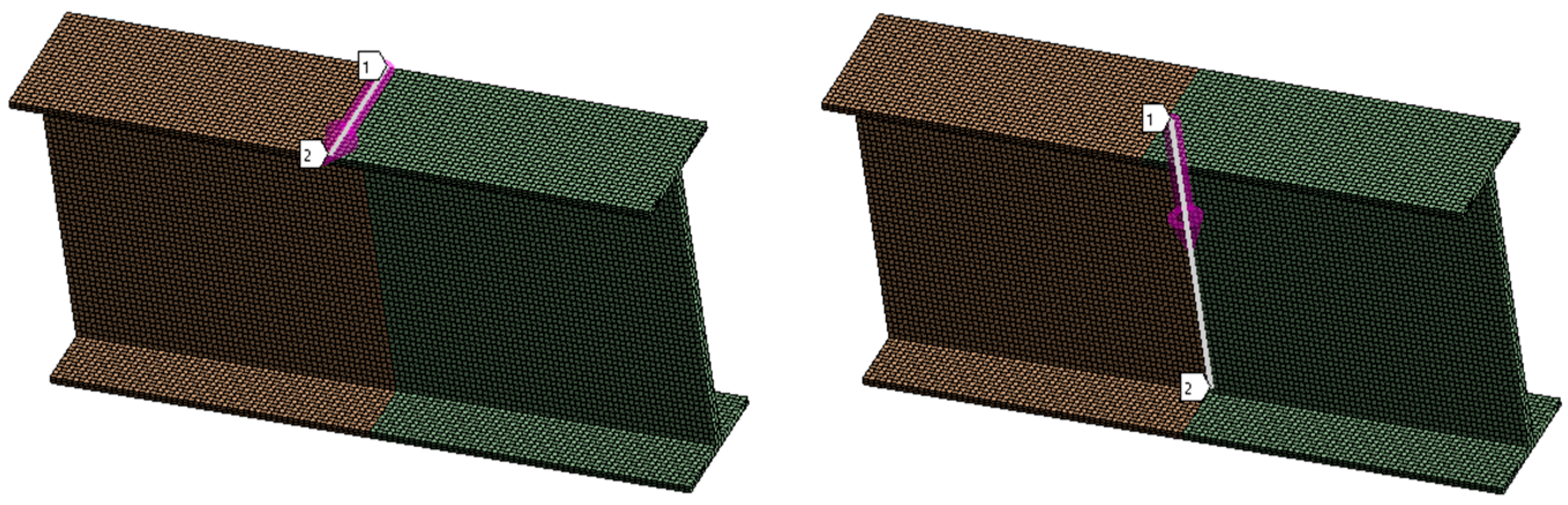
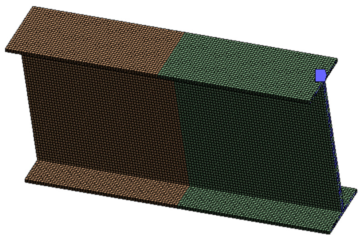
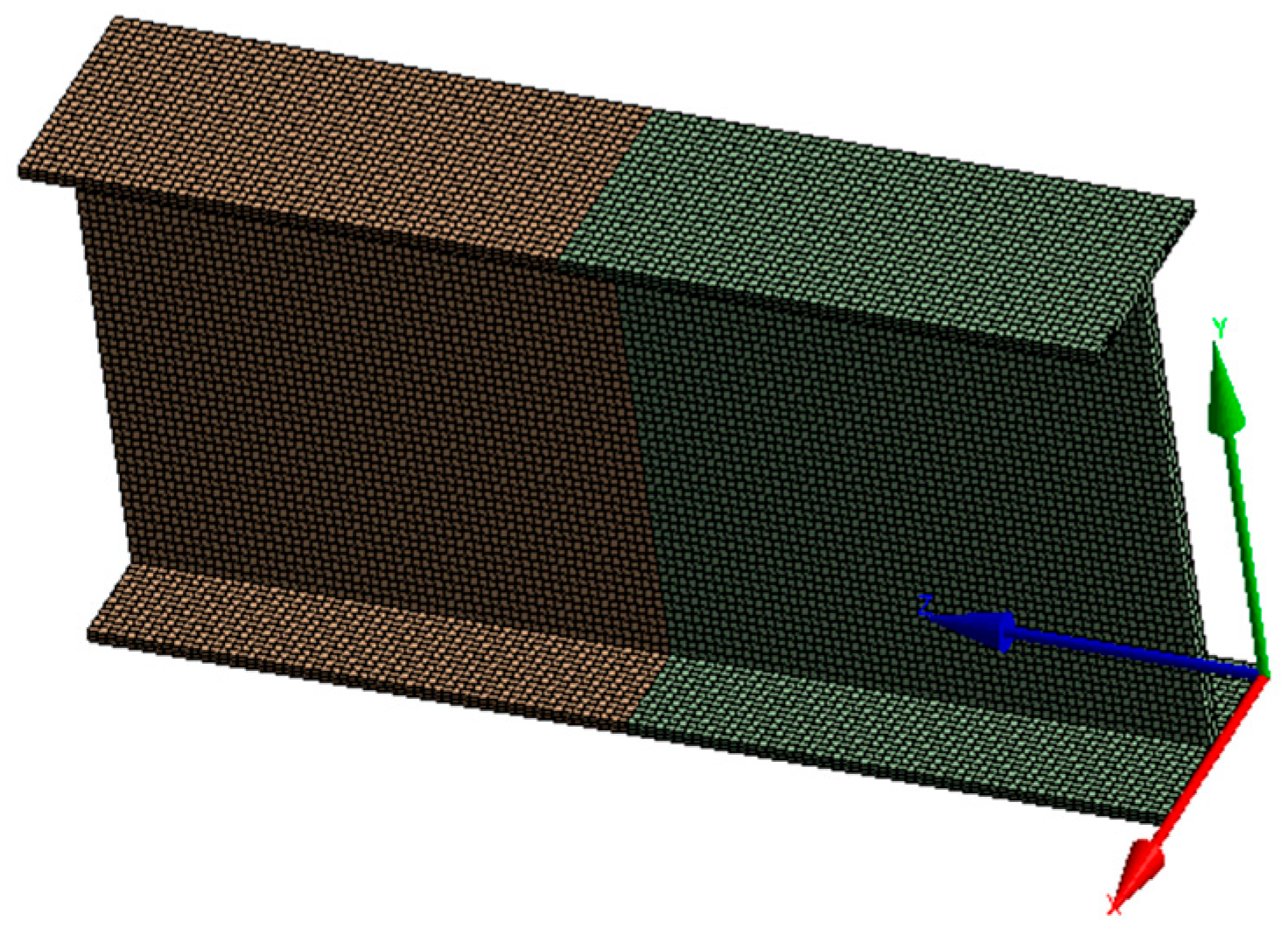
Take working condition 2 as an example. This case represents a typical H-beam with dimensions 900 mm flange width, 400 mm web height, 20 mm flange thickness, 35 mm web thickness, and total length 2000 mm, formed by welding two sections along the flange-web joint. To avoid rigid body displacement and residual stress release in the structural analysis, displacement constraints are imposed on the sides. The coordinate system, boundary conditions, and meshing are shown in Figure 1, Figure 2 and Figure 3.

3. Welding Heat Source

The establishment of a heat source model in the weld area is a key step in the realization of numerical simulation of welding, which can represent the energy distribution of the heat source more accurately and will directly affect the accuracy of the prediction of the temperature field and residual stress field in the weld area. The spatial distribution of heat source energy in arc welding is significantly non-uniform, and the Gaussian heat source model is used to characterize heat source energy. Although the double ellipsoidal model [9] is more accurate for deep penetration, for the H-beam thicknesses considered in this study (≤35 mm) and the computational efficiency required for parametric studies, the Gaussian model provides sufficient accuracy with lower cost. The Gaussian heat source model can measure the spatial distribution characteristics of the heat flux density as a continuous function and can effectively characterize the dynamic behavior of the arc hot spot. The distribution characteristics of the heat flux density follow a two-dimensional Gaussian distribution, and the relationship is as follows:

$$Q(r)=Q\times {\mathrm{e}}^{-({\displaystyle \frac{3r^2}{R^2}})}$$

(1)

In the formula, Q(r) is heat flux density at a radial distance r from the center of the heat source; Q is maximum heat flux density at the center of the heat source, and R is the effective heating radius of the arc; r is the distance from any point in the area where the heat source acts to the center of the heat source. The physical meaning of this model is that arc energy is released at the center of the hot spot and decays exponentially in all directions, which is consistent with the energy distribution characteristics formed in the molten pool during actual welding. Compared with the double ellipsoidal heat source model, the Gaussian model is more efficient in single-pass welding simulation calculations and is applicable to butt welding calculations for both thin and medium-thick plates.

As for simplifications regarding phase transformation and latent heat, in this study, phase transformation effects and latent heat are not considered. For Q235 structural steel, the solid-state phase transformation (austenite to ferrite/pearlite) occurs during cooling, which can introduce transformation-induced plasticity (TRIP) and affect residual stress development. However, for the thickness range (≤35 mm) and welding parameters considered, the thermal cycles are relatively short and the contribution of transformation strains to the final residual stress is secondary to thermal contraction. Moreover, the inclusion of latent heat would require a coupled thermal-metallurgical model, significantly increasing computational cost without proportionally improving accuracy for the parametric trends investigated. This simplification is commonly adopted in welding simulation studies focusing on process parameter effects, and its influence is expected to be minor for the comparative analysis presented in this work.

In the actual welding process, the heat source migrates continuously with the movement of the welding torch, and its spatial position changes over time: $X_0,Y_0$. To reproduce this dynamic process, this study builds a mobile Gaussian heat source loading module based on ANSYS APDL parametric programming technology. In each time increment step, dynamic loading was implemented on the action surface based on the heat flux density function of the Gaussian distribution, with the geometric center of the welding heat source () as the action origin. With the spatial migration of the heat source, the area and distribution parameters of the heat flux in each loading step are updated synchronously; $r^2={(X-X_0)}^2+{(Y-Y_0)}^2$. By adjusting key parameters such as the heat source action radius and peak heat flux density to make them change continuously with the advancement of the time increment step, the heat action process of the moving heat source is accurately reproduced, and the numerical simulation of the welding transient temperature field is achieved. Based on the aforementioned theoretical derivations, the mathematical expression of the constructed Gaussian heat source migration model is:

$$Q(R)=Q\times {\mathrm{e}}^{[-3\times {\displaystyle \frac{(X-X_0{)}^2+{(Y-\mathit{vt}-Y_0)}^2}{R^2}}]}$$

(2)

In the formula, X₀ and Y₀ are respectively the coordinates of the geometric center of the welding heat source; v is the welding speed; t is the welding duration.

4. Result Analysis

4.1. Working Condition 2 Welding Temperature Field

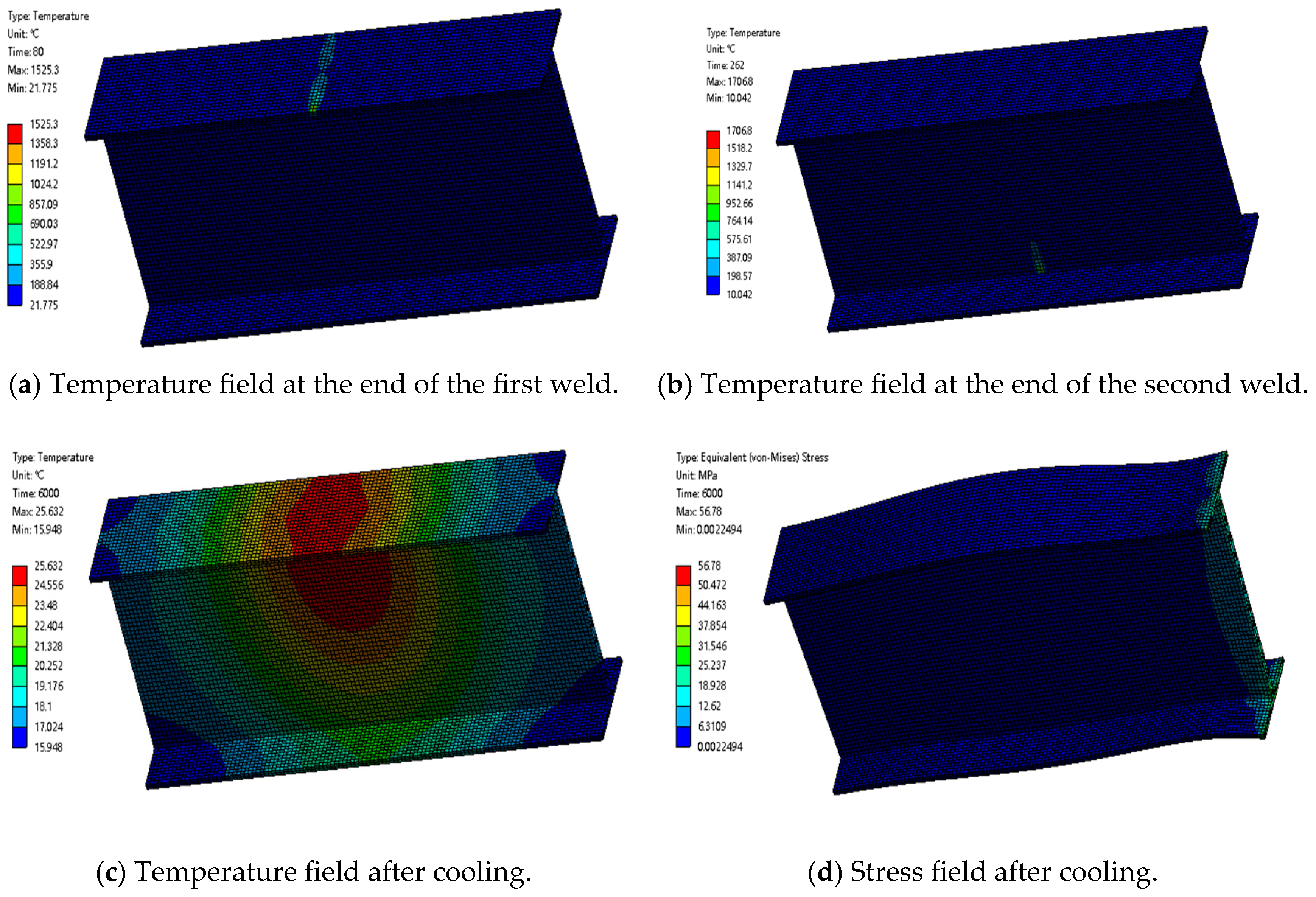
Taking Condition 2 as an example, this condition represents the baseline parameter set (I = 210 A, v = 5 mm/s) and is used to illustrate the typical temperature field evolution. The temperature field distributions at the end of the first and second welds, as well as the temperature field and stress field distributions when cooled to 6000 s, are shown in Figure 4.

Figure 4 shows the heat transfer behavior and residual stress distribution on the surface of H-shaped steel butt joints during welding with a moving Gaussian heat source. It can be observed that, although the heat source is in the process of continuous movement, the distribution of heat flux density generated by the heat source remains stable. This is because in the area where the heat source acts, the mode of energy transfer does not change significantly but has certain static characteristics. And it has a similar heat transfer pattern in space and time.

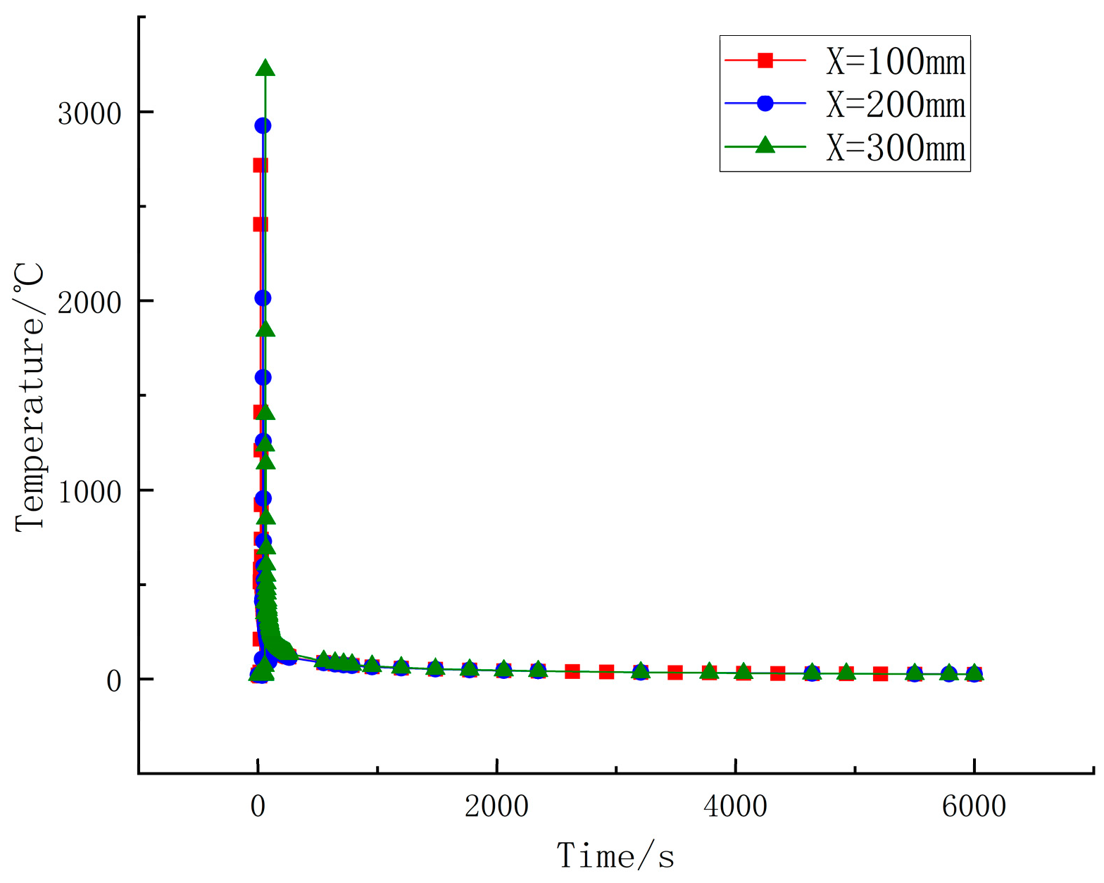
It can be observed from Figure 5 and Figure 6 that at a certain point under the action of a moving heat source, the temperature will increase steeply to the high point and then slowly fall back to the normal temperature point, presenting typical characteristics of a general transient; and the rate of increase in heating is significantly greater than the rate of decrease in cooling, showing an asymmetric temperature–time response. In addition, in three-dimensional space, it is perpendicular to the cross-section of the weld seam, and the farther away from the midline of the weld seam, the higher the gradient of the temperature response.

4.2. Fitting Relationship Between Welding Residual Stress and Welding Time, Temperature and So On

Viscoelastic-plastic constitutive models considering thermal cycles and deformation history are currently advanced and accurate methods for simulating welding stresses. They are not a single formula but a framework model system that includes multiple equations describing the material’s behavior at different temperatures.

$$\mathsf{\sigma }=\mathrm{F}(\mathsf{\epsilon }\_\mathrm{total},\mathsf{\epsilon }\_\mathrm{plastic},\mathsf{\epsilon }\_\mathrm{creep},\mathrm{T},\mathrm{T}\_\mathrm{history},\dots )$$

(3)

Here, ε_plastic and ε_creep are calculated by the elastic–plastic model and creep model, respectively, both closely related to temperature T and time t. Compared with the ideal elastic–plastic model, it can more accurately reflect the real mechanical behavior of materials under welding thermal cycles, making the simulated residual stress and deformation more consistent with theoretical results.

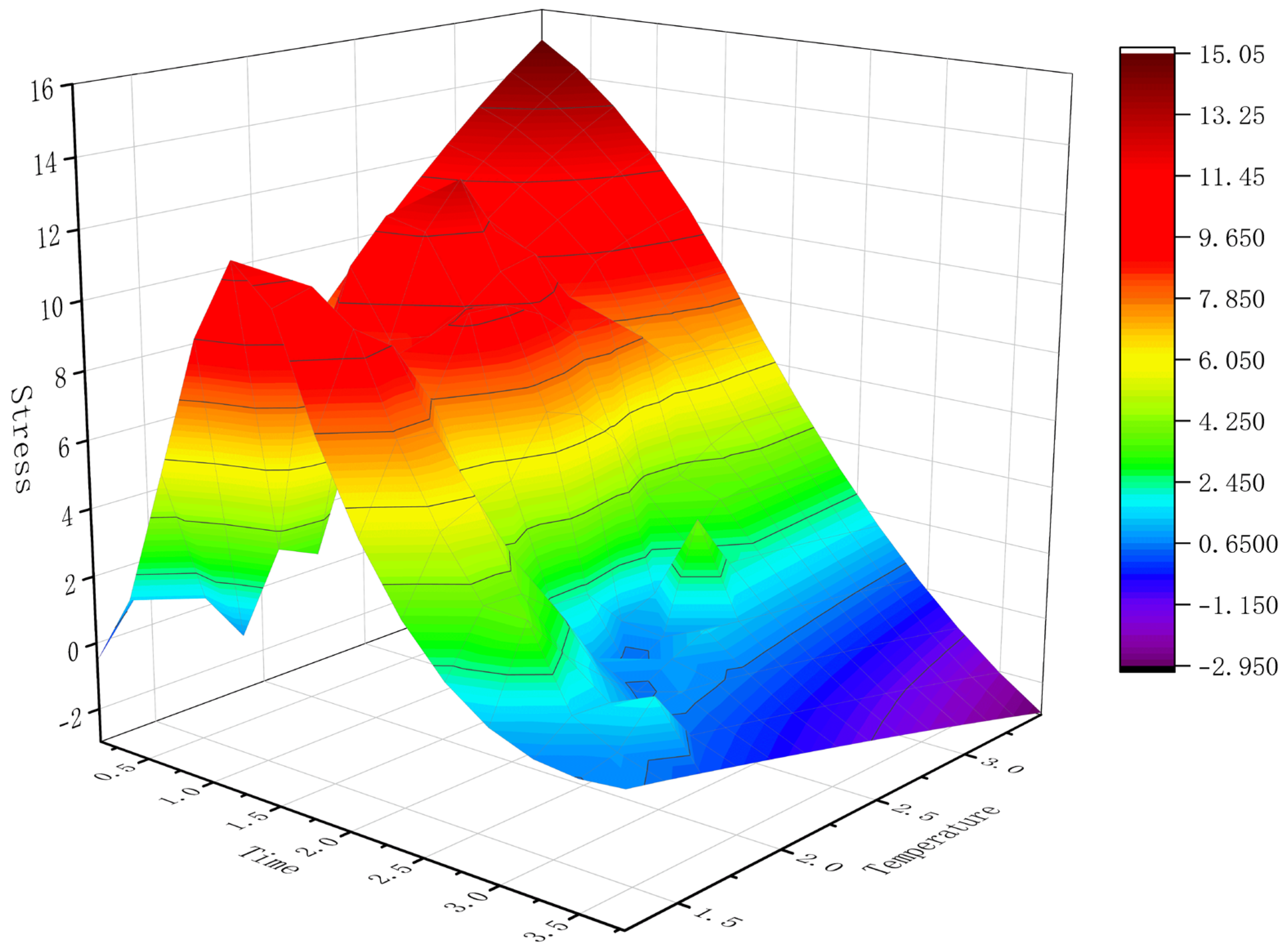
Through nonlinear regression analysis of the simulation data of the cooling stage in case two, it was found that the welding residual stress (σ) has a significant power function relationship with time (t) and temperature (T), which can be approximately expressed by the following empirical formula:

$$\sigma =k\ast t^{-0.8}\ast T^{0.1}$$

(4)

where k is a material constant. The temperature exponent 0.1 reflects the mild sensitivity of residual stress to temperature during cooling, as at lower temperatures yield strength increases and stress relaxation slows. The fitting relationship between welding residual stress and welding time and temperature is as shown in Figure 7. This relationship indicates that welding stress has a strong time attenuation effect and slightly increases with temperature, which is consistent with the physical mechanism of stress relaxation; under high-temperature short-time conditions, the material’s yield strength decreases and creep effects are significant, resulting in a lower stress level; while under low-temperature long-time conditions, stress gradually decays with time. It should be noted that this empirical model has a large fitting deviation in the heating stage because it fails to fully reflect the complex factors such as phase transformation, material nonlinearity, and transient thermo-mechanical coupling during the welding process. To achieve higher accuracy in prediction, subsequent research will adopt the finite element method based on the thermoelastic–plastic theory or introduce constitutive models considering phase transformation plasticity for multi-physics field coupling simulation to more accurately reveal the stress evolution law throughout the welding process.

In addition, geometric parameters significantly influence residual stress distribution. Meanwhile, in the three-dimensional welding model, the thickness and aspect ratio of the component are also key geometric parameters that affect the temperature field gradient and the distribution of residual stress. An increase in thickness will lengthen the heat conduction path, causing heat to accumulate in the thickness direction, which reduces cooling rate in the welding area, thereby enhancing the three-dimensional thermal constraint effect and promoting a non-uniform distribution of residual stress in the thickness direction. According to the numerical simulation results of different thickness specimens in this study, when thickness increases from 20 mm to 35 mm, the peak temperature at the center of the weld seam rises by approximately 8%, while the peak value of residual tensile stress shows a nonlinear decreasing trend with the increase in thickness. Additionally, an increase in the aspect ratio significantly enhances the influence of the boundary effect on the uniformity of the temperature field. In specimens with an aspect ratio greater than 2.5, heat during the welding process is more likely to diffuse along the length, resulting in a reduction in the lateral temperature gradient and a more uniform distribution of residual stress. Simulation data shows that when the aspect ratio increases from 1.5 to 3.0, the peak value of lateral residual stress decreases by approximately 12%, indicating that a reasonable design of the component’s aspect ratio can effectively alleviate the concentration of welding stress.

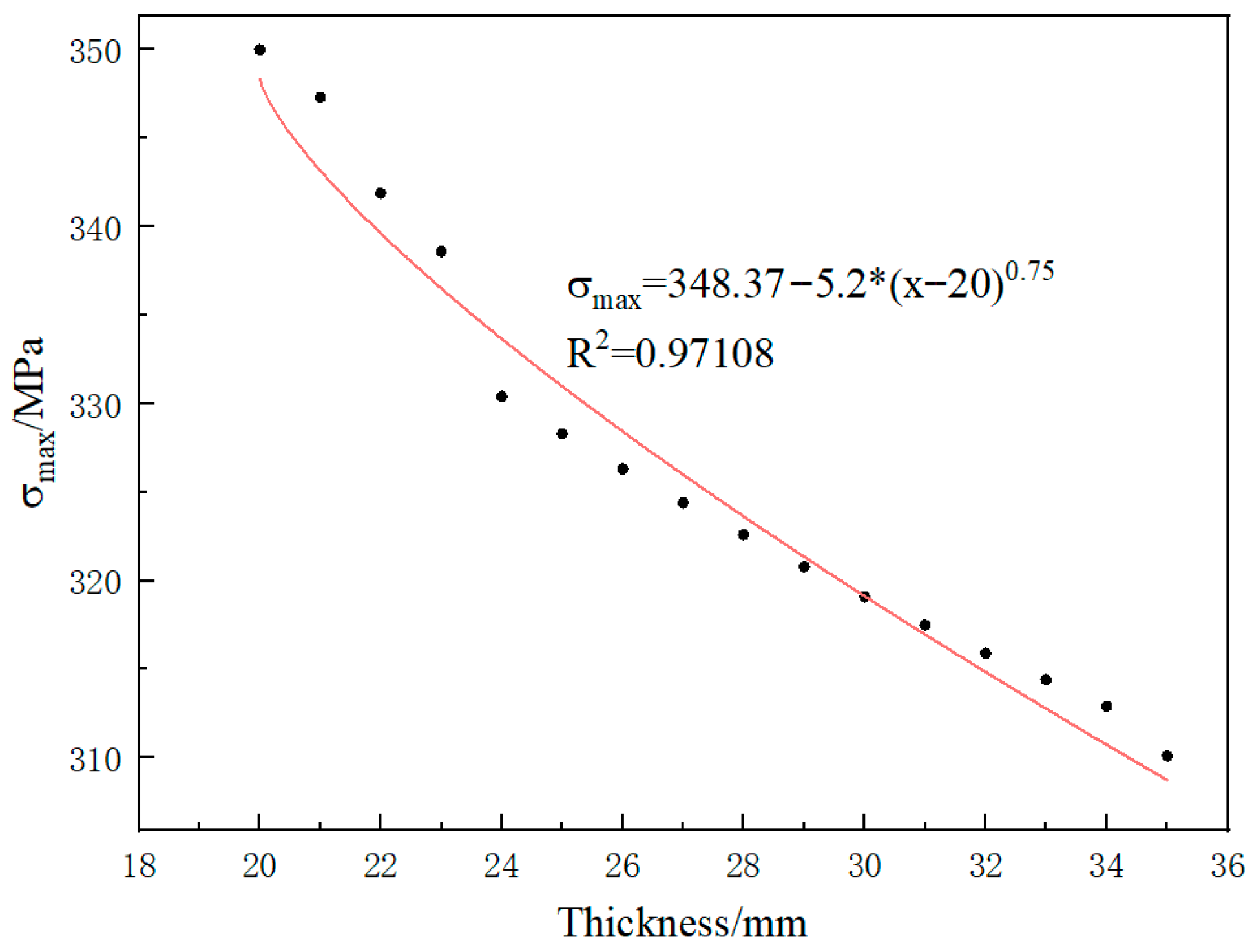
To further quantify the influence of geometric dimensions, based on the numerical simulation data, scatter plots of the fitting relationship between thickness, aspect ratio, and the peak value of residual stress were drawn, as shown in Figure 8, which shows the influence of thickness (t) on peak longitudinal residual stress (σ_max) at the center of the weld seam. The distribution of data points indicates that peak residual stress decreases in a nonlinear manner as thickness increases. Through nonlinear regression analysis, the fitting formula is obtained as follows:

$${\mathsf{\sigma }}_{\max }=348.37-5.2\times (\mathrm{x}-20{)}^{0.75}$$

(5)

The coefficient of determination R² of this formula is approximately 0.97108, indicating a high degree of fit. Error analysis shows that within the thickness range of 20–35 mm, the mean absolute error (MAE) between the predicted and simulated values is ±7.3 MPa, with maximum deviation occurring around 23 mm (about 12 MPa), which may be related to the specific balance point reached by three-dimensional constraints and cooling rate at this thickness.

The observed nonlinear decrease in peak residual stress with thickness is consistent with general trends reported in the welding literature for thick-section joints, where increasing thickness enhances three-dimensional thermal constraints and reduces the effectiveness of stress relaxation. However, direct quantitative comparison with previous studies on H-beams is limited, as most existing work has focused on simple butt or T-joints. The fitted formula presented in this study provides new quantitative insight for medium-thickness H-beams (20–35 mm) that has not been previously reported.

4.3. The Influence of the Welding Heat Source on Welding Residual Stress and Temperature

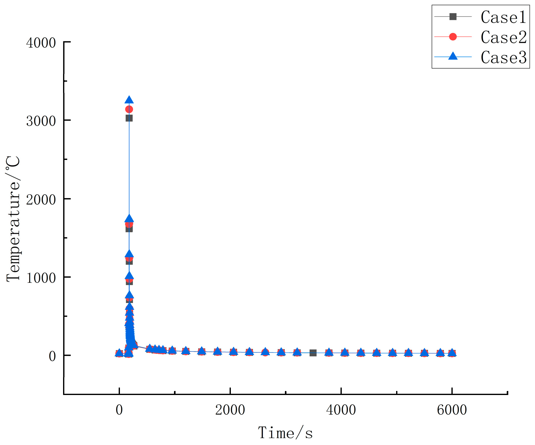
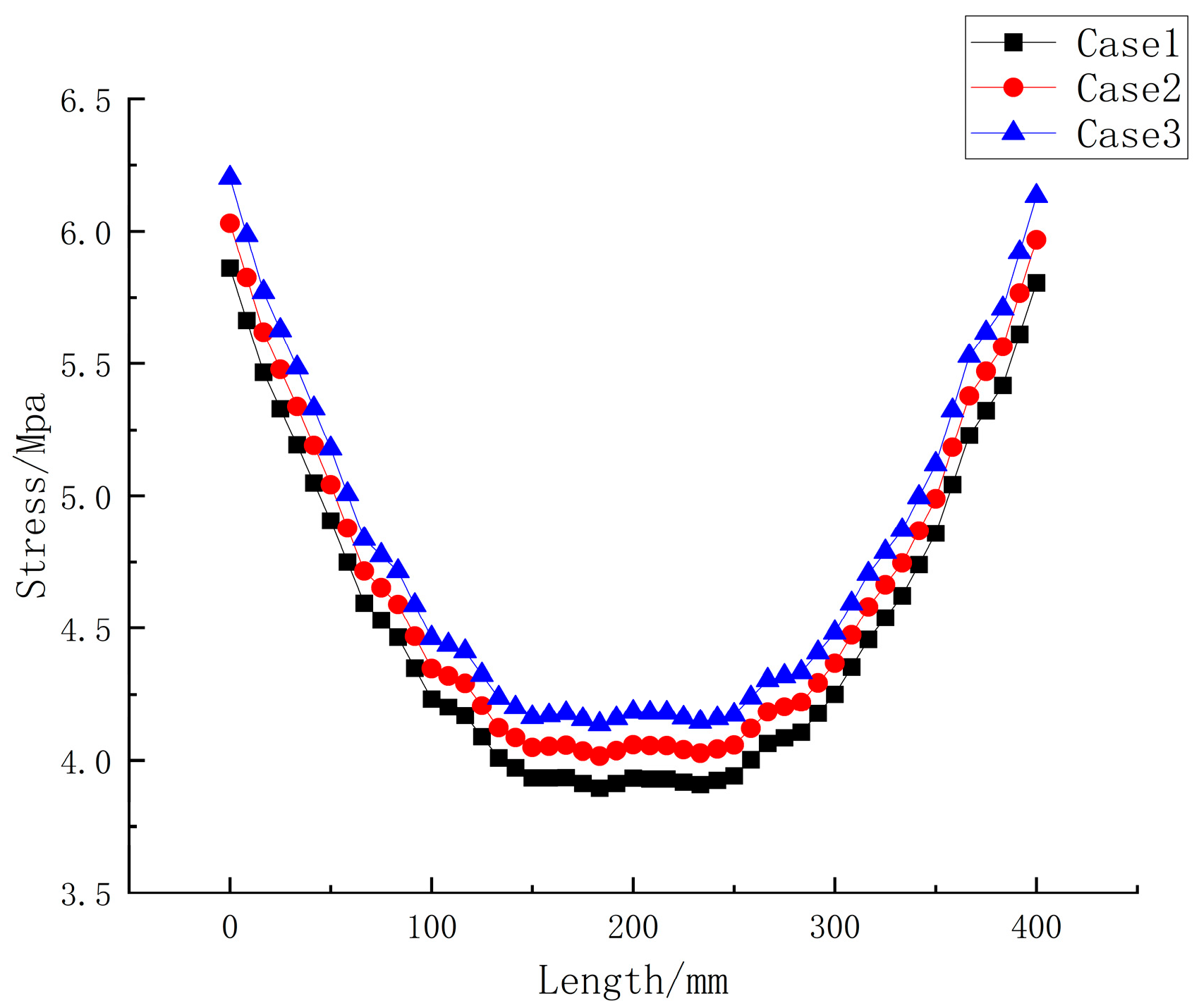
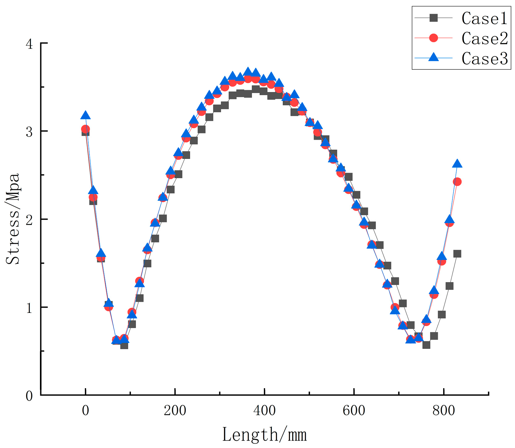
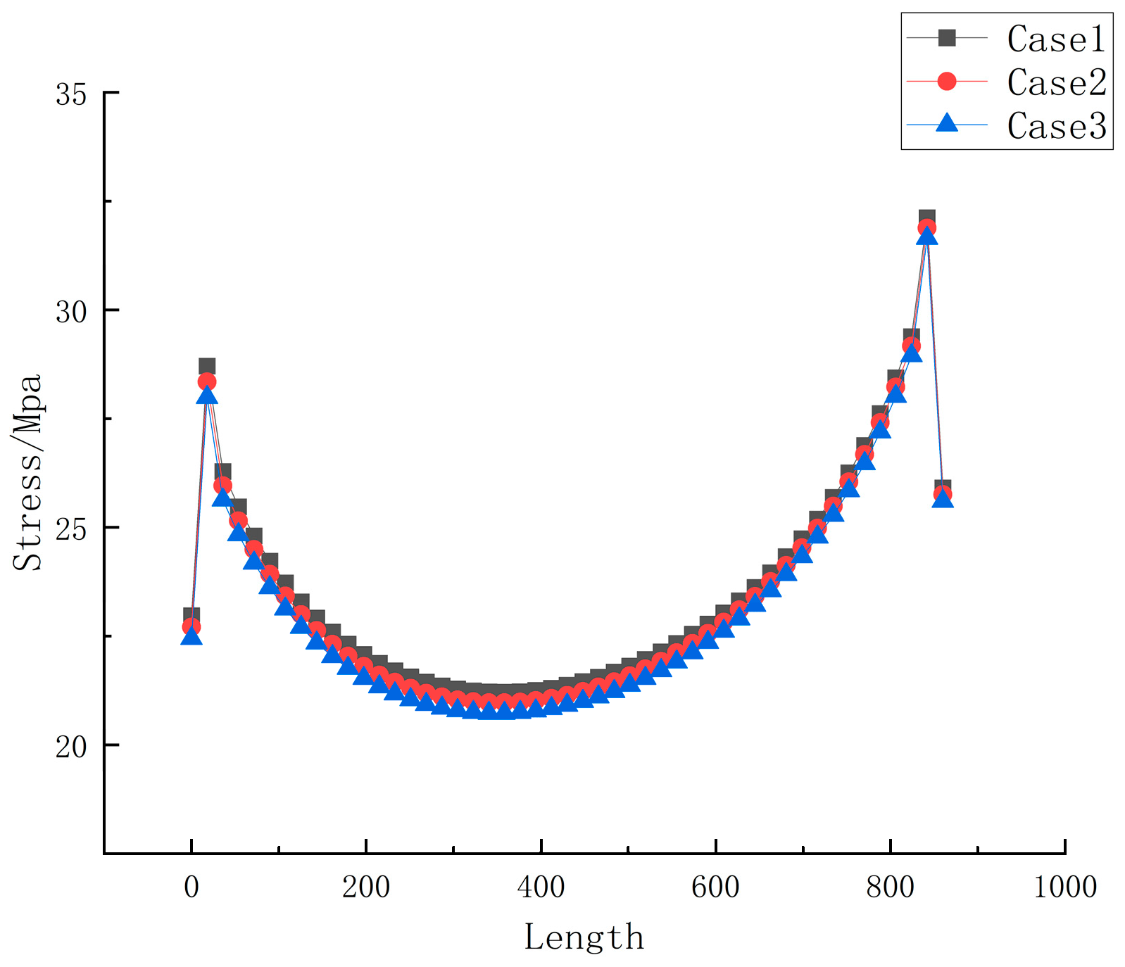
The temperature cycling curves corresponding to different welding heat sources are shown in Figure 9, and the residual stress distribution corresponding to the centerline path of the weld seam corresponding to the same welding heat source is shown in Figure 10 and Figure 11. Analysis reveals that within the same thickness range, while other welding process parameters remain unchanged, the welding current is proportional to the peak temperature field. When the welding current increased from 200 A to 220 A, the peak temperature increased by about 10% (from 1850 °C to 2035 °C), and the peak residual stress of the two weld seams increased by about 5% (from 320 MPa to 336 MPa) and 3% (from 315 MPa to 324 MPa) respectively. It was also found that within the range of the welding current, although the distribution curve of the residual stress remained unchanged, the maximum longitudinal residual stress of the weld seam increased with the increase of the welding current. For every 10A increase in welding current, the rate of increase in peak residual stress decreases from 1.4% to 0.4%, showing a nonlinear decreasing trend.

4.4. Effects of Welding Speed on Welding Residual Stress and Temperature

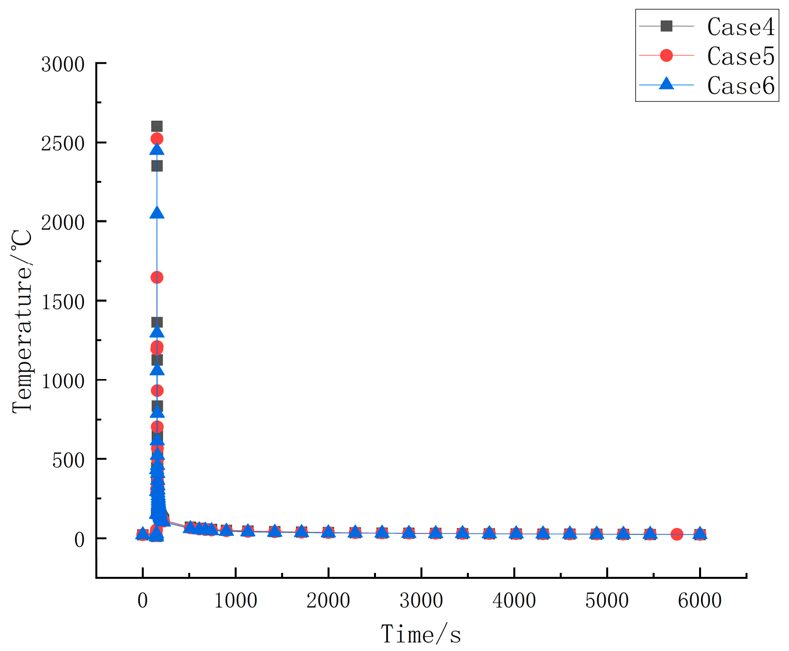
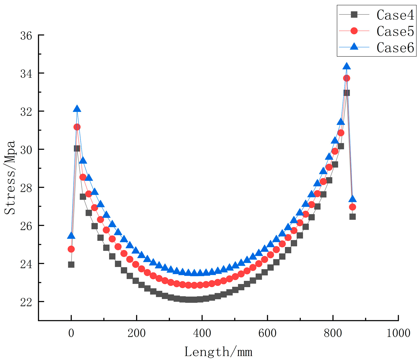
The temperature cycling curves corresponding to different welding speeds are shown in Figure 12, and the distribution of weld centerline residual stress corresponding to different welding speeds is shown in Figure 13 and Figure 14. It can be seen from the figure that under the same conditions, as the welding speed of the component decreases and the peak of the temperature field gradually increases. The distribution pattern of the welding residual stress is basically stable but the decrease in welding speed leads to a significant increase in the peak value of the residual stress in the weld direction. It is important to clarify the relationship: increasing welding speed reduces residual stress. For example, when speed increases from 6 mm/s to 8 mm/s, peak residual stress decreases by about 20% (from 350 MPa to 280 MPa).

4.5. Boundary Effects of Welded Components

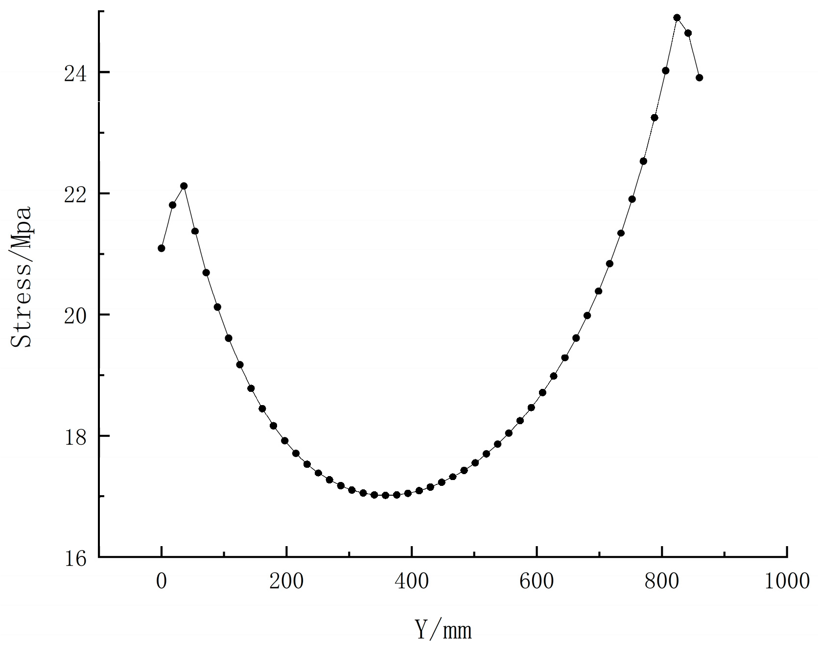
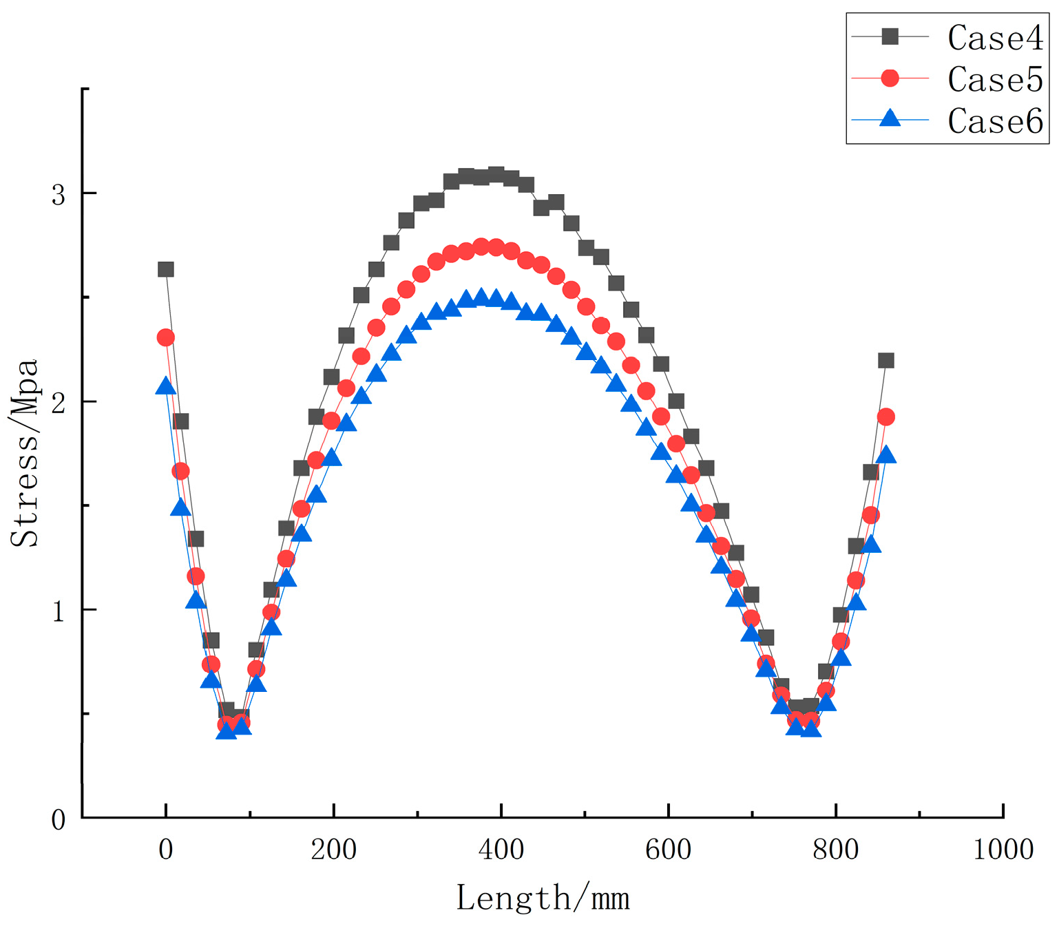
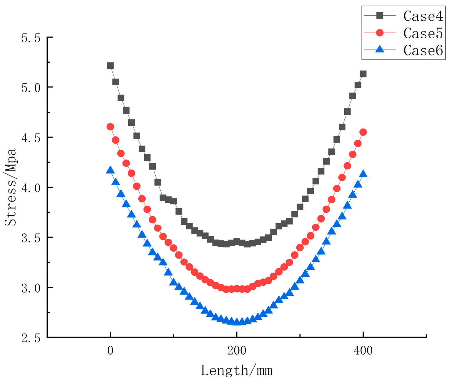
The residual stress distribution along the centerline path of the weld seam corresponding to different welding heat sources is shown in Figure 15 and the residual stress distribution along the centerline path of the weld seam corresponding to different welding speeds is shown in Figure 16. Analysis reveals that the distribution pattern of residual stress at the boundary is opposite to that at the weld. The results show that the residual stress field of H-beam welding exhibits typical self-balancing distribution characteristics. Higher longitudinal and transverse residual tensile stress was generated in the weld center and heat-affected zone due to restrained contraction during cooling. However, obvious residual compressive stress was observed in the component boundary area. This phenomenon is attributed to the fact that the component as a whole must satisfy the internal force balance condition: the contraction tension generated in the weld zone needs to be transmitted through the component and balanced by corresponding compressive stress in the boundary area. This boundary effect is particularly pronounced in complex cross-section components such as H-beams, as the flanges and webs provide a specific stiffness distribution and force transmission path. The summary is shown in

Table 3. Summary of key simulation results under different welding parameters.

Case	I (A)	v (mm/s)	Peak Temperature (°C)	Peak Longitudinal Residual Stress (MPa)
1	200	5	1850	320
2	210	5	1950	329
3	220	5	2035	336
4	210	6	1893	350
5	210	7	1824	301
6	210	8	1750	280

.

5. Conclusions

Based on the numerical simulations of H-shaped steel welding, the following conclusions are drawn:

(1) Peak temperature increases with welding current and decreases with welding speed. Increasing current from 200 A to 220 A raises the peak temperature by about 10% (from 1850 °C to 2035 °C), while increasing speed from 5 mm/s to 8 mm/s reduces it by approximately 18% (from 1950 °C to 1750 °C).

(2) Residual stress is significantly affected by both parameters. Raising current from 200 A to 220 A increases the peak longitudinal residual stress by about 5% (from 320 MPa to 336 MPa). In contrast, increasing speed from 6 mm/s to 8 mm/s reduces peak residual stress by approximately 20% (from 350 MPa to 280 MPa).

(3) Geometric parameters also influence residual stress. Increasing plate thickness from 20 mm to 35 mm leads to a nonlinear decrease in peak residual stress (up to 12%), with a fitted relationship. Increasing the aspect ratio from 1.5 to 3.0 reduces lateral residual stress by approximately 12%.

(4) Boundary effects produce compressive stresses at the component edges, balancing the tensile stresses in the weld zone and demonstrating the self-equilibrating nature of the residual stress field.

(5) A combination of lower heat input and higher welding speed is recommended for minimizing residual stress, provided full penetration is ensured. Future work will consider welding voltage, external loads, and cyclic loading effects.

Based on the ANSYS Workbench platform, this paper uses thermodynamic coupling to simulate the welding process of H-shaped steel joints. A sensitivity comparison shows that increasing the welding current by 10 A raises the peak residual stress by approximately 1.4% to 0.4%, whereas increasing the welding speed by 1 mm/s reduces the peak residual stress by approximately 8% to 10%. This indicates that welding speed has a more pronounced effect on residual stress reduction than current within the parameter range studied. Through numerical simulation of models with different heat sources and different welding speeds, the influence laws of welding heat sources and welding speeds on the welding temperature field and residual stress under certain welding parameters are analyzed. The test shows that under the condition of fixed welding parameters, the higher the welding current during the welding process, the higher the highest point of the temperature field, and the temperature peak is positively correlated with the welding current; The lower the welding speed, the higher the peak in the temperature field, and the temperature peak is negatively correlated with the welding speed; and as the weld decreases, the maximum residual stress in the cooled weld area increases. The next step is to study variables such as welding voltage and external load and analyze the effect of these variables on the release of residual stress in the weldment and impact on the safety of the entire welded component under cyclic loading. Future work will incorporate phase transformation effects, consider position-dependent welding conditions, and extend the analysis to cyclic loading scenarios.