Author Contributions
Conceptualization, H.L. and G.Z.; methodology, H.L.; software, H.L. and L.W.; validation, H.L., L.W., Q.Z. and H.X.; formal analysis, H.L. and Q.Z.; investigation, H.L. and L.W.; resources, G.Z. and H.X.; data curation, H.L. and Q.Z.; writing—original draft preparation, H.L.; writing—review and editing, G.Z. and H.X.; visualization, H.L.; supervision, G.Z. and H.X.; project administration, G.Z.; funding acquisition, G.Z. and H.X. All authors have read and agreed to the published version of the manuscript.
Figure 1.
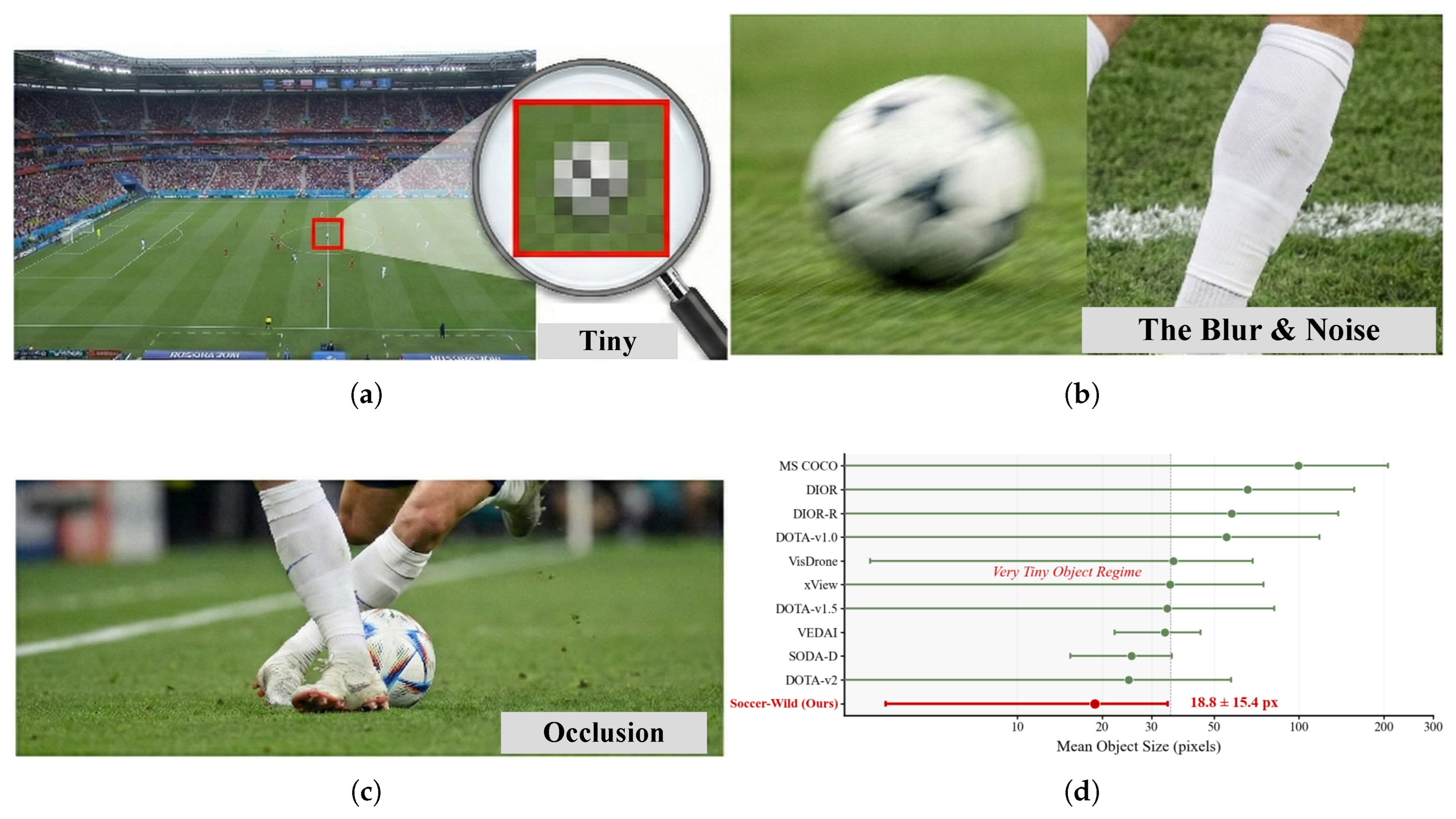
Visual challenges in unconstrained soccer ball detection and statistical comparison of the proposed benchmark. (a) The Scale Dilemma: Illustrates the extreme scale variation in wide-angle broadcast footage. The target often occupies fewer than pixels (less than 0.1% of the frame), causing severe feature erosion during downsampling. (b) Blur & Noise: Depicts visual degradations where high-speed motion induces severe blur, rendering shape priors ineffective, while background clutter (e.g., player socks) introduces visual ambiguity. (c) The Occlusion: Shows a typical scenario where the target is partially or fully obstructed by players, challenging standard geometric localization. (d) Object Size Comparison: A quantitative analysis of mean object sizes across prominent detection datasets. Our Soccer-Wild benchmark (highlighted in red) falls strictly within the Very Tiny Object Regime with a mean size of pixels, presenting a significantly higher difficulty level compared to general (e.g., MS COCO) and aerial (e.g., VisDrone) datasets.
Figure 1.
Visual challenges in unconstrained soccer ball detection and statistical comparison of the proposed benchmark. (a) The Scale Dilemma: Illustrates the extreme scale variation in wide-angle broadcast footage. The target often occupies fewer than pixels (less than 0.1% of the frame), causing severe feature erosion during downsampling. (b) Blur & Noise: Depicts visual degradations where high-speed motion induces severe blur, rendering shape priors ineffective, while background clutter (e.g., player socks) introduces visual ambiguity. (c) The Occlusion: Shows a typical scenario where the target is partially or fully obstructed by players, challenging standard geometric localization. (d) Object Size Comparison: A quantitative analysis of mean object sizes across prominent detection datasets. Our Soccer-Wild benchmark (highlighted in red) falls strictly within the Very Tiny Object Regime with a mean size of pixels, presenting a significantly higher difficulty level compared to general (e.g., MS COCO) and aerial (e.g., VisDrone) datasets.

Figure 2.
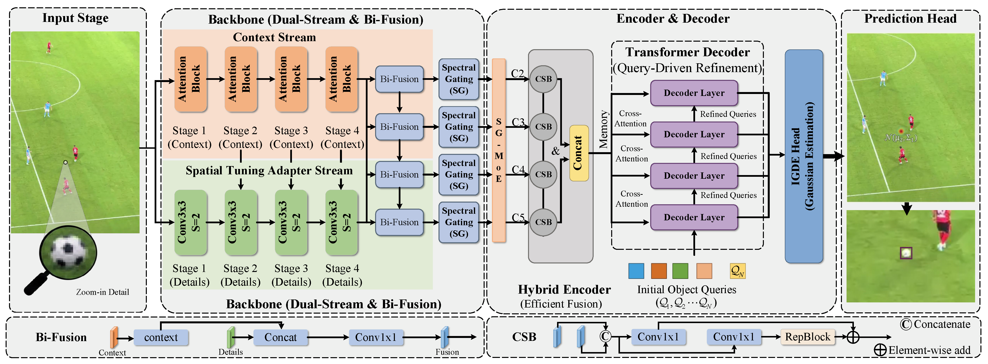
The overall architecture of the proposed GOAL framework. The pipeline operates in a coarse-to-fine manner to maintain structural integrity across four integral stages: Dual-Stream Backbone & Bi-Fusion: The input image is processed via parallel Context and Spatial Tuning Adapter streams to decouple global semantic symmetry and local spatial details, which are interactively synchronized via Bi-Fusion modules. Frequency-aware Spectral Gating (SG): The fused features undergo spectral purification in the Fourier domain to suppress low-frequency background redundancies while amplifying target-specific structural singularities. Hybrid Encoder & Decoder: A Multi-Granularity Mixture of Experts (MG-MoE), integrated within the Hybrid Encoder, dynamically routes features based on motion states to address anisotropic distortions. The Transformer Decoder then performs query-driven refinement to align sparse features into a consistent latent space. Prediction Head: The IGDE Head leverages Information Entropy to estimate the target’s location as a radially symmetric Gaussian distribution , recovering weak signals through probabilistic modeling. The bottom panels detail the internal architectures of the Bi-Fusion and CSB modules, emphasizing the hierarchical balance of the framework.
Figure 2.
The overall architecture of the proposed GOAL framework. The pipeline operates in a coarse-to-fine manner to maintain structural integrity across four integral stages: Dual-Stream Backbone & Bi-Fusion: The input image is processed via parallel Context and Spatial Tuning Adapter streams to decouple global semantic symmetry and local spatial details, which are interactively synchronized via Bi-Fusion modules. Frequency-aware Spectral Gating (SG): The fused features undergo spectral purification in the Fourier domain to suppress low-frequency background redundancies while amplifying target-specific structural singularities. Hybrid Encoder & Decoder: A Multi-Granularity Mixture of Experts (MG-MoE), integrated within the Hybrid Encoder, dynamically routes features based on motion states to address anisotropic distortions. The Transformer Decoder then performs query-driven refinement to align sparse features into a consistent latent space. Prediction Head: The IGDE Head leverages Information Entropy to estimate the target’s location as a radially symmetric Gaussian distribution , recovering weak signals through probabilistic modeling. The bottom panels detail the internal architectures of the Bi-Fusion and CSB modules, emphasizing the hierarchical balance of the framework.

Figure 3.
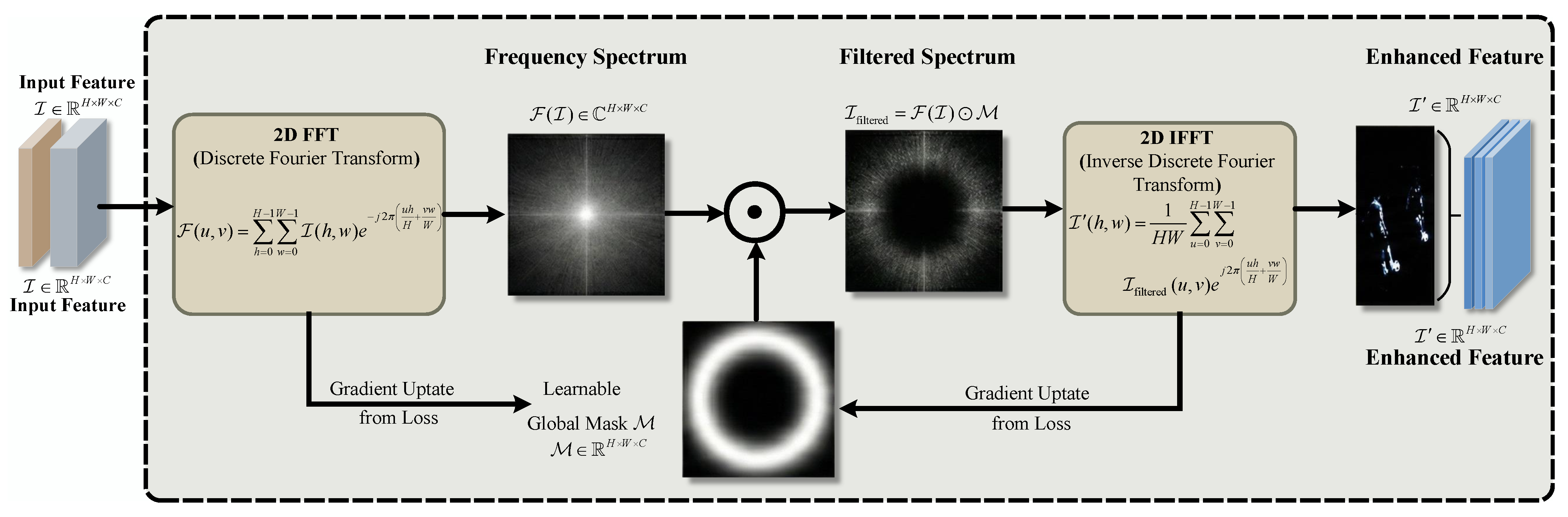
Illustration of the Frequency-aware Spectral Gating (SG) module. The input feature is transformed into the frequency domain via 2D FFT. A learnable global mask is then applied to the spectrum to filter out background noise. Finally, the enhanced feature is reconstructed via 2D IFFT, effectively purifying the target signal.
Figure 3.
Illustration of the Frequency-aware Spectral Gating (SG) module. The input feature is transformed into the frequency domain via 2D FFT. A learnable global mask is then applied to the spectrum to filter out background noise. Finally, the enhanced feature is reconstructed via 2D IFFT, effectively purifying the target signal.
Figure 4.
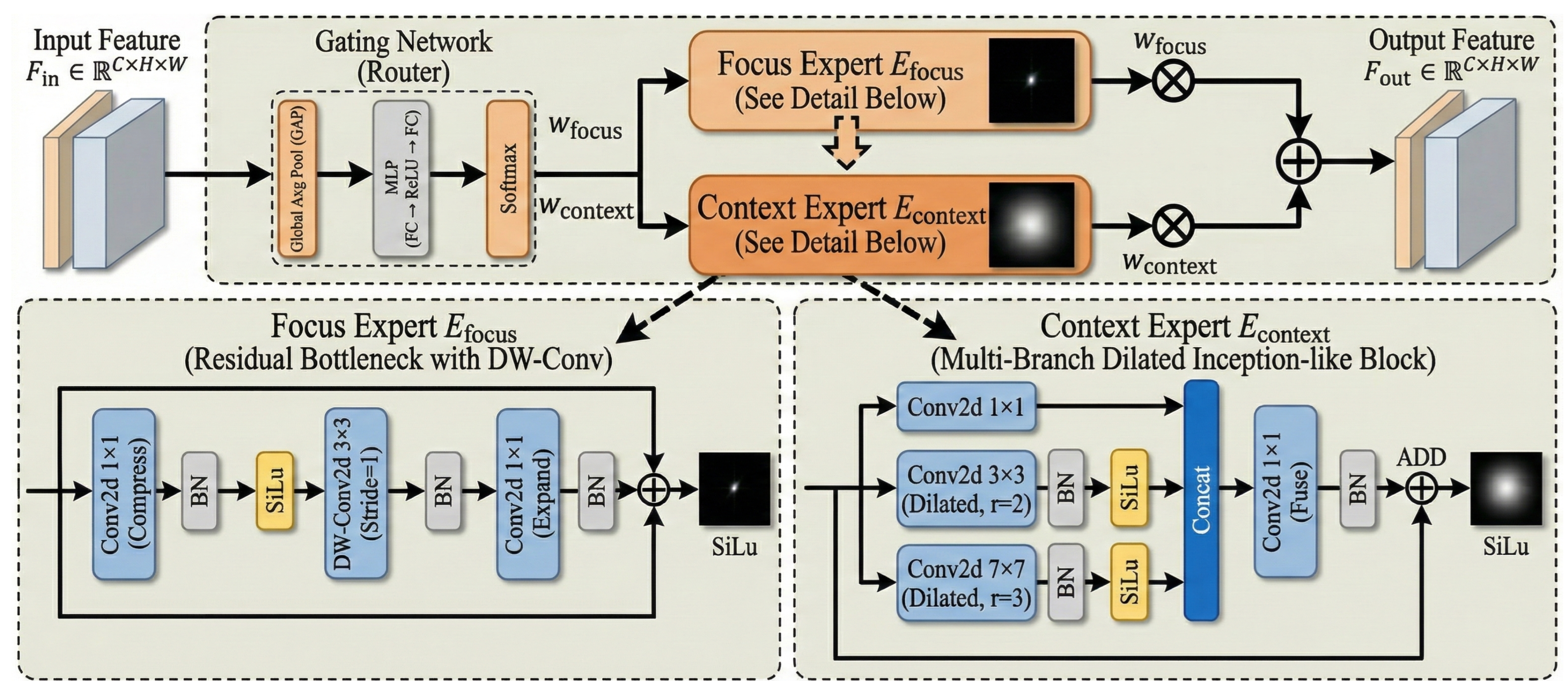
Architecture of the Multi-Granularity Mixture of Experts (MG-MoE) module. The Gating Network dynamically assigns weights () to route features. The Focus Expert (bottom left) uses residual bottlenecks to extract sharp details, while the Context Expert (bottom right) employs dilated convolutions to capture blurred motion context. The final output is obtained via adaptive weighted fusion.
Figure 4.
Architecture of the Multi-Granularity Mixture of Experts (MG-MoE) module. The Gating Network dynamically assigns weights () to route features. The Focus Expert (bottom left) uses residual bottlenecks to extract sharp details, while the Context Expert (bottom right) employs dilated convolutions to capture blurred motion context. The final output is obtained via adaptive weighted fusion.
Figure 5.
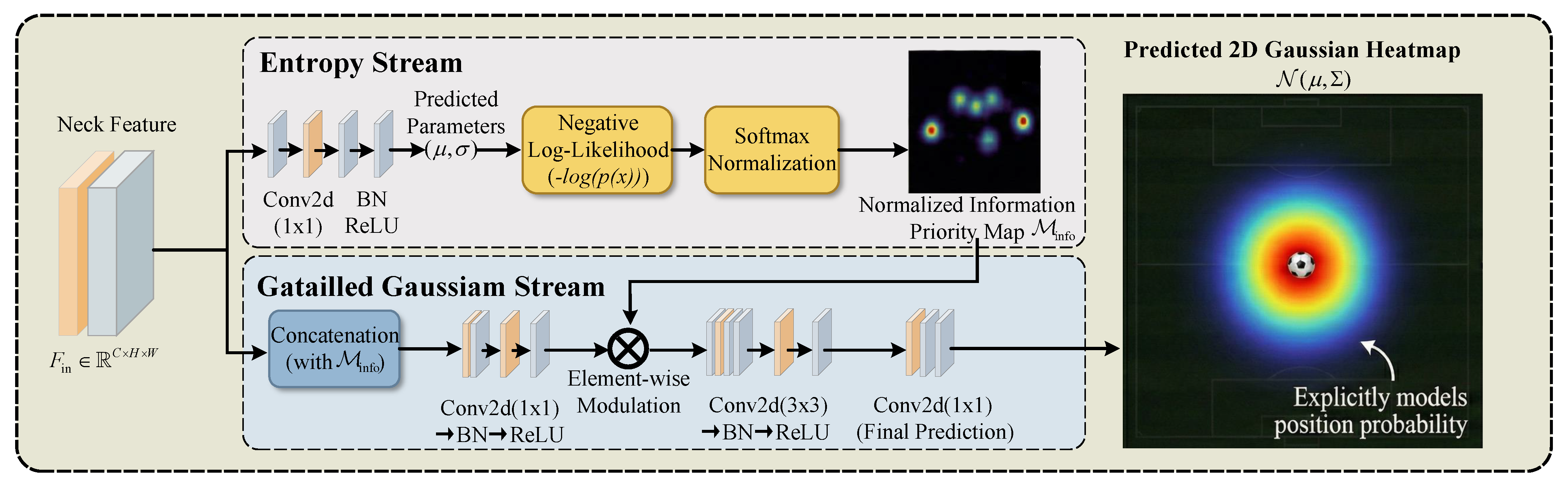
Schematic of the Information-Guided Gaussian Distribution Estimation (IGDE) module. Instead of deterministic regression, IGDE utilizes an self-guided Information Entropy Map to identify salient regions. These priors guide the network to model the tiny target as a probabilistic 2D Gaussian distribution , effectively recovering eroded features. The colorful radial gradient represents the modeled location probability distribution, where the warm colors (red and orange) indicate high-probability target regions at the center, while the cool colors (blue) represent very low probability areas towards the outer edges.
Figure 5.
Schematic of the Information-Guided Gaussian Distribution Estimation (IGDE) module. Instead of deterministic regression, IGDE utilizes an self-guided Information Entropy Map to identify salient regions. These priors guide the network to model the tiny target as a probabilistic 2D Gaussian distribution , effectively recovering eroded features. The colorful radial gradient represents the modeled location probability distribution, where the warm colors (red and orange) indicate high-probability target regions at the center, while the cool colors (blue) represent very low probability areas towards the outer edges.
Figure 6.
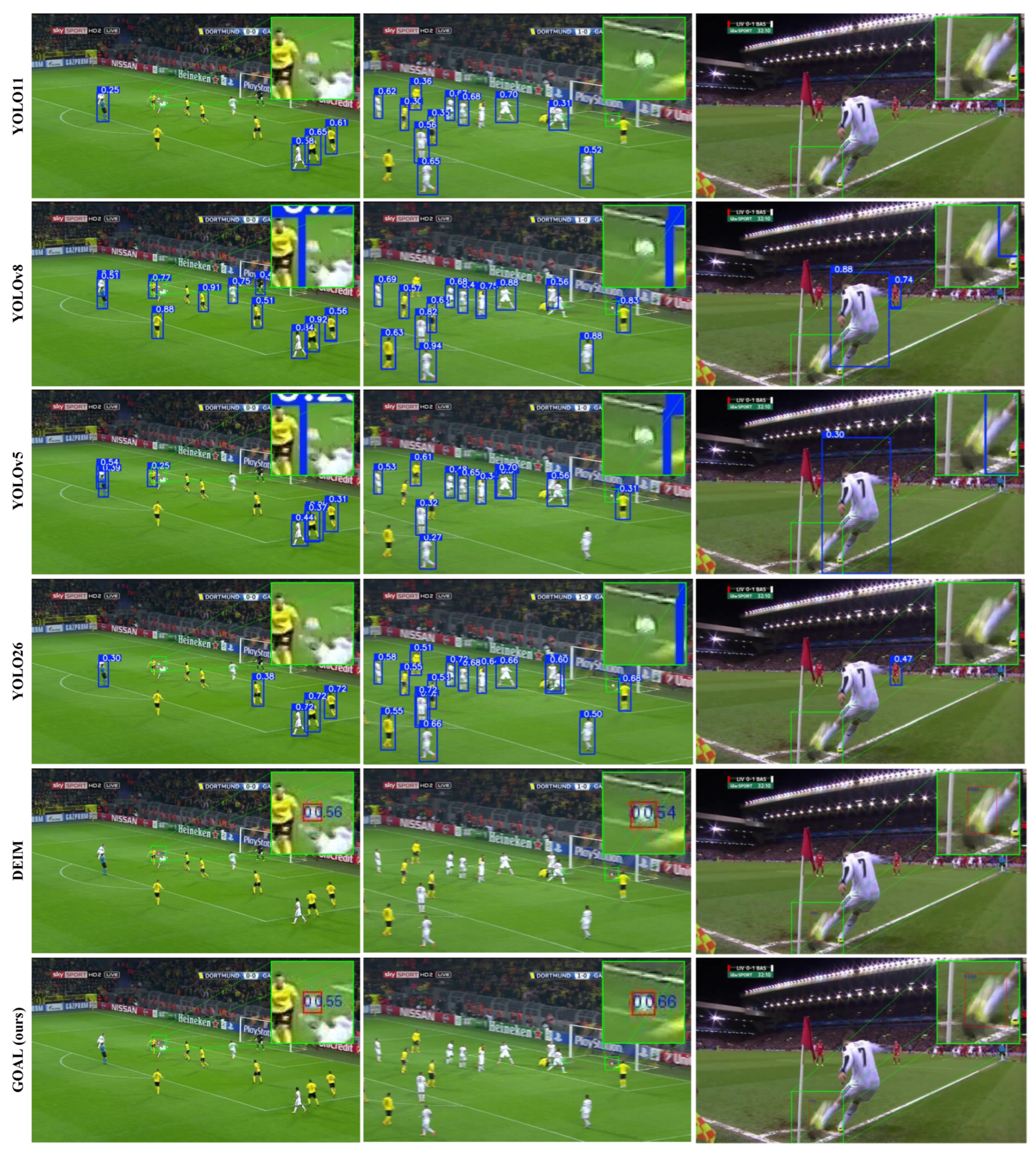
Qualitative comparison on the Soccer-Wild test set. Compared with state-of-the-art generic detectors (e.g., YOLO series) and DEIM, our GOAL (bottom row) demonstrates superior robustness in locating the tiny, fast-moving soccer ball under challenging conditions such as motion blur and background clutter. In the visualization, the green boxes indicate zoomed-in regions for a clearer view of the micro-scale targets. The blue bounding boxes represent detections from baseline methods (which often detect players or generate false positives), while the red bounding boxes highlight the accurate localization of the soccer ball by our proposed GOAL model.
Figure 6.
Qualitative comparison on the Soccer-Wild test set. Compared with state-of-the-art generic detectors (e.g., YOLO series) and DEIM, our GOAL (bottom row) demonstrates superior robustness in locating the tiny, fast-moving soccer ball under challenging conditions such as motion blur and background clutter. In the visualization, the green boxes indicate zoomed-in regions for a clearer view of the micro-scale targets. The blue bounding boxes represent detections from baseline methods (which often detect players or generate false positives), while the red bounding boxes highlight the accurate localization of the soccer ball by our proposed GOAL model.
Figure 7.
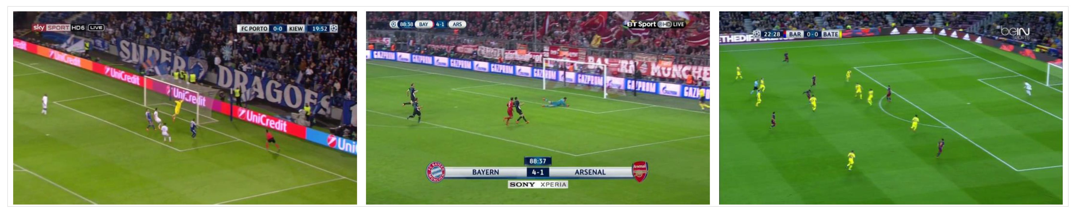
Typical failure cases of the GOAL framework. False negatives occur under extreme visual degradations: (Left) extreme background clutter, (Middle) zero-contrast blending with the goal net, and (Right) extreme scale degradation. The severe loss of spatial contrast in these single-frame scenarios deprives the overall framework of reliable visual cues.
Figure 7.
Typical failure cases of the GOAL framework. False negatives occur under extreme visual degradations: (Left) extreme background clutter, (Middle) zero-contrast blending with the goal net, and (Right) extreme scale degradation. The severe loss of spatial contrast in these single-frame scenarios deprives the overall framework of reliable visual cues.
Table 1.
Comparison of Soccer-Wild with existing object detection datasets.
Table 1.
Comparison of Soccer-Wild with existing object detection datasets.
| Dataset | Pub. | Year | Image Height | Image Count | Type | Object Size |
|---|
| MS COCO [41] | ECCV | 2014 | 800–1333 | 163,957 | HBB | |
| DIOR [42] | P&RS | 2020 | 800 | 23,463 | HBB | |
| DIOR-R [42] | P&RS | 2020 | 800 | 23,463 | OBB | |
| DOTA-v1.0 [10] | CVPR | 2018 | 800–13,000 | 2423 | H/OBB | |
| VisDrone [9] | ICCVW | 2018 | 2000 | 8629 | HBB | |
| xView [43] | arXiv | 2018 | 3000 | 1127 | HBB | |
| DOTA-v1.5 [40] | TPAMI | 2019 | 800–13,000 | 2423 | H/OBB | |
| DOTA-v2 [40] | TPAMI | 2021 | 800–13,000 | 11,268 | H/OBB | |
| VEDAI (512) [44] | JVCIR | 2015 | 512, 1024 | 1210 | HBB | |
| SODA-D [12] | TPAMI | 2023 | 3407 | 24,828 | OBB | |
| Soccer-Wild (ours) | - | 2026 | 416–1080 | 14,773 | HBB | |
Table 2.
Benchmarking results on the proposed Soccer-Wild test set. The best results are highlighted in bold, and the second best are underlined.
Table 2.
Benchmarking results on the proposed Soccer-Wild test set. The best results are highlighted in bold, and the second best are underlined.
| Method | Year | Pub. | Backbone | Params (M) | GFLOPs | mAP | AP50 | AP75 |
|---|
| FRCNN [48] | 2015 | ICCV | ResNet-50 | 41.35 | 185.50 | 27.45 | 49.80 | 26.10 |
| SSD [49] | 2016 | ECCV | VGG-16 | 26.28 | 61.32 | 19.85 | 38.50 | 18.20 |
| YOLOv5 [50] | 2020 | Github | CSPDarknet | 9.12 | 24.04 | 24.80 | 52.43 | 23.38 |
| YOLOv6 [51] | 2022 | arXiv | CSPDarknet | 16.31 | 44.21 | 30.43 | 55.47 | 28.06 |
| YOLOv8 [52] | 2023 | Github | CSPDarknet | 11.14 | 28.65 | 30.93 | 61.05 | 25.77 |
| YOLOv9 [53] | 2024 | ECCV | GELAN | 7.29 | 27.39 | 28.22 | 54.03 | 19.03 |
| YOLOv10 [54] | 2024 | NeurIPS | CSPDarknet | 8.07 | 24.77 | 30.82 | 58.86 | 24.94 |
| YOLO11 [55] | 2024 | Github | - | 9.43 | 21.55 | 28.63 | 56.38 | 21.20 |
| YOLOv12 [56] | 2025 | NeurIPS | R-ELAN | 9.25 | 21.52 | 28.80 | 54.25 | 23.77 |
| YOLO26 [57] | 2026 | arXiv | - | 9.95 | 22.50 | 31.25 | 60.41 | 25.38 |
| RT-DETR [7] | 2024 | CVPR | ResNet-50 | 42.76 | 130.47 | 27.66 | 55.23 | 22.16 |
| D-FINE [46] | 2025 | ICLR | ResNet-50 | 9.85 | 24.50 | 31.95 | 61.50 | 27.10 |
| DEIM [47] | 2025 | CVPR | ResNet-50 | 10.23 | 20.55 | 32.6 | 71.5 | 25.7 |
| GOAL (Ours) | - | - | MG-MoE | 12.41 | 29.66 | 40.0 | 77.9 | 33.9 |
Table 3.
Quantitative comparison with state-of-the-art detectors on the VisDrone2019 benchmark.
Table 3.
Quantitative comparison with state-of-the-art detectors on the VisDrone2019 benchmark.
| Method | Year | Pub. | Backbone | AP95 | AP50 | FPS |
|---|
| FRCNN [48] | 2015 | ICCV | Hourglass | 21.8 | 41.8 | 17 |
| CornerNet [58] | 2018 | ECCV | ResNet-50 | 17.4 | 34.1 | - |
| ARFP [59] | 2022 | Appl. Intell. | ResNet-50 | 20.4 | 33.9 | - |
| DMNet [60] | 2020 | CVPRW | ResNet-50 | 29.4 | 49.3 | - |
| DSHNet [61] | 2021 | WACV | ResNet-50 | 30.3 | 51.8 | - |
| CRENet [62] | 2020 | ECCV | ResNet-50 | 33.7 | 54.3 | - |
| YOLOv5 [50] | 2020 | GitHub | CSPDarknet | 21.9 | 42.3 | 85 |
| YOLOv7 [63] | 2023 | CVPR | CSPDarknet | 23.0 | 41.1 | 55 |
| TPH-YOLOv5 [64] | 2021 | ICCV | CSPDarknet | 23.1 | 41.5 | 25 |
| YOLOv8 [52] | 2023 | GitHub | CSPDarknet | 25.5 | 42.1 | 90 |
| HIC-YOLOv5 [65] | 2024 | ICRA | CSPDarknet | 26.0 | 44.3 | - |
| YOLO-DCTI [66] | 2023 | Remote Sens. | CSPDarknet | 27.4 | 49.8 | 15 |
| Drone-YOLO-L [67] | 2023 | Drones | CSPDarknet | 31.9 | 51.3 | - |
| DAU-YOLO-L [45] | 2025 | Remote Sens. | CSPDarknet | - | 43.8 | 24.6 |
| Deformable-DETR [68] | 2020 | arXiv | ResNet-50 | 27.1 | 43.1 | 19 |
| RT-DETR [7] | 2024 | CVPR | ResNet-50 | 27.7 | 45.8 | 76 |
| Drone-DETR [69] | 2024 | Sensor | ResNet-50 | 33.9 | 53.9 | 30 |
| GOAL (Ours) | 2026 | - | MG-MoE | 40.4 | 55.1 | 28 |
Table 4.
Component-wise effectiveness analysis on the Soccer-Wild dataset. SG: Spectral Gating; MG-MoE: Multi-Granularity Mixture of Experts; IGDE: Information-Guided Gaussian Distribution Estimation. The baseline is DEIM [
47] with a ResNet-50 backbone.
Table 4.
Component-wise effectiveness analysis on the Soccer-Wild dataset. SG: Spectral Gating; MG-MoE: Multi-Granularity Mixture of Experts; IGDE: Information-Guided Gaussian Distribution Estimation. The baseline is DEIM [
47] with a ResNet-50 backbone.
| Exp. | SG | MG-MoE | IGDE | mAP | AP50 | AP75 |
|---|
| 1 | - | - | - | 32.6 | 71.5 | 25.7 |
| 2 | ✔ | - | - | 36.4 (+3.8) | 75.2 (+3.7) | 29.8 (+4.1) |
| 3 | ✔ | ✔ | - | 38.2 (+5.6) | 76.5 (+5.0) | 32.1 (+6.4) |
| 4 | ✔ | - | ✔ | 38.9 (+6.3) | 77.1 (+5.6) | 32.9 (+7.2) |
| 5 | ✔ | ✔ | ✔ | 40.0 (+7.4) | 77.9 (+6.4) | 33.9 (+8.2) |
Table 5.
Ablation study on Expert Design and Granularity. We compare the standard CNN block, MLP-based mixing block, Homogeneous Experts, and our Heterogeneous MG-MoE. Our method achieves the best trade-off between parameter efficiency and detection accuracy.
Table 5.
Ablation study on Expert Design and Granularity. We compare the standard CNN block, MLP-based mixing block, Homogeneous Experts, and our Heterogeneous MG-MoE. Our method achieves the best trade-off between parameter efficiency and detection accuracy.
| Exp. | Expert Design | Params | mAP | AP50 |
|---|
| 1 | Standard ResNet Block | 11.25 M | 36.4 | 75.2 |
| 2 | MLP-Mixer Block (Dense) | 14.80 M | 36.9 | 75.6 |
| 3 | Homogeneous MoE () | 12.15 M | 37.3 | 75.9 |
| 4 | MG-MoE (Heterogeneous) | 12.35 M | 38.2 | 76.5 |
Table 6.
Ablation on the Number of Experts (N) in MG-MoE. We evaluate different combinations of Focus () and Context () experts. achieves the best balance between efficiency and accuracy, while suffers from slight overfitting.
Table 6.
Ablation on the Number of Experts (N) in MG-MoE. We evaluate different combinations of Focus () and Context () experts. achieves the best balance between efficiency and accuracy, while suffers from slight overfitting.
| Total Experts (N) | Configuration | Params (M) | GFLOPs | mAP | AP50 |
|---|
| 2 | 1 Focus + 1 Context | 11.85 | 28.82 | 37.4 | 75.8 |
| 4 (Default) | 2 Focus + 2 Context | 12.41 | 29.66 | 38.2 | 76.5 |
| 6 | 3 Focus + 3 Context | 30.08 | 23.45 | 38.1 | 76.3 |
Table 7.
Sensitivity analysis of the Gaussian Kernel Radius in IGDE. We investigate the impact of fixed radius settings versus our adaptive strategy.
Table 7.
Sensitivity analysis of the Gaussian Kernel Radius in IGDE. We investigate the impact of fixed radius settings versus our adaptive strategy.
| Exp. | Radius Strategy | Value | mAP | AP50 |
|---|
| 1 | Fixed (Very Strict) | | 34.2 | 71.5 |
| 2 | Fixed (Small) | | 36.1 | 73.8 |
| 3 | Fixed (Optimal) | | 37.8 | 76.1 |
| 4 | Fixed (Medium) | | 37.6 | 75.9 |
| 5 | Fixed (Large) | | 36.8 | 75.1 |
| 6 | Fixed (Very Large) | | 35.2 | 72.4 |
| 7 | Adaptive (Ours) | | 38.2 | 76.5 |
Table 8.
Sensitivity analysis of the IGDE loss weight . We vary the weight of the auxiliary loss to find the optimal balance. Setting yields the best performance, while excessively large weights dominate the main detection task, leading to performance degradation.
Table 8.
Sensitivity analysis of the IGDE loss weight . We vary the weight of the auxiliary loss to find the optimal balance. Setting yields the best performance, while excessively large weights dominate the main detection task, leading to performance degradation.
| Exp. | Loss Weight () | mAP | AP50 |
|---|
| 1 | 0.0 | 37.3 | 75.8 |
| 2 | 0.1 | 37.6 | 76.0 |
| 3 | 0.5 | 38.0 | 76.3 |
| 4 | 1.0 (Ours) | 38.2 | 76.5 |
| 5 | 2.0 | 37.9 | 76.2 |
| 6 | 5.0 | 36.5 | 74.9 |