Symmetry-Aware Continual Learning for Dynamic Dimensional Multivariate Time Series Forecasting: Integrating Redundancy Clustering and Multi-LoRA Adapters

Abstract

Continual learning of multivariate time series (MTS) forecasting is critical for process industries where working condition drift is frequent due to the variation in the feed properties and other factors. However, existing continual learning methods struggle with dynamic input dimension changes, and the lack of symmetry-aware feature and dimension regulation further exacerbates the interference of irrelevant variables and dimensional inconsistency. To overcome this problem, G-MLoRA, a continual learning method based on dynamic redundancy clustering and multiple low-rank adapters, is proposed in this paper. This method can effectively enhance the network’s capability for prediction of multivariate time series under dynamic input dimensions. First, it groups MTS via Wasserstein distance-K-means clustering to reduce irrelevant variable interference. Second, each group is assigned to an exclusive LoRA adapter, with pre-trained backbone weights frozen during fine-tuning to lower complexity and mitigate catastrophic forgetting. Third, mini-batch gradient accumulation enables reuse of inconsistent-dimensional historical knowledge. Extensive experiments on two real grinding classification datasets show G-MLoRA outperforms baselines in new/historical knowledge compatibility, especially under dynamic dimensions.

1. Introduction

Efficient and stable multivariate time series forecasting is an effective technology to assist process perception and predictive control in process industries. In recent years, deep learning technologies represented by Transformers have gradually become a research focus in multivariate time series modeling for process industries due to their strong capabilities in learning long-term sequence dependencies and high-dimensional complex relationships [1]. Although many studies [2,3,4] have explored ways to improve the prediction performance of deep neural networks on multivariate time series forecasting in process industries through offline training and network structure optimization, practical applications face inevitable challenges. Changes and fluctuations in material properties and production plans, wear to equipment and failure of sensors continuously alter the numerical distribution of process variables and the relationships between them. This leads to a gradual decline or even complete failure of neural networks trained offline over time. Taking the grinding classification process as an example, as mining depth and location gradually change, the properties of the ore, the main input material of the process, will inevitably change continuously over time. Additionally, the operation and wear status of equipment will also change over time. These factors lead to dynamic temporal changes in the overall distribution and interrelationships of variables such as concentration, particle size, and mill efficiency, i.e., working condition drift. As the degree of such drift gradually increases, the performance of time series prediction models built solely on overly outdated historical data will inevitably decline or even fail completely. Therefore, continual learning methods that enable neural networks to constantly adapt to data characteristics under new operating conditions have emerged as a key focus in both application and research.

In most current continual learning studies for time series, catastrophic forgetting caused by incremental learning has been extensively discussed. Direct full-parameter fine-tuning of pre-trained models using new data significantly degrades the model’s prediction ability on historical knowledge and impairs its generalization performance. To address this issue, experience replay [5] is a widely adopted strategy. It caches a portion of historical data and uses both new and historical data as the training set during each fine-tuning process, allowing the network to balance new and historical knowledge in continual learning. Based on pure instance-based experience replay, it was found that by integrating knowledge distillation [6], which treats the hidden features outputted by intermediate neurons as part of historical experience when the network predicts historical data, the proposed method can further enhance the compatibility between new and old knowledge [7,8,9]. Study [10] added a moving average of historical weights to experience replay. However, for long-term and variable continual learning tasks in process industries, strategies which rely solely on the experience replay faces a trade-off between computational efficiency and learning performance [11]. Study [12] proposed targeted replay of samples with the most significant prediction performance degradation. Additionally, researchers have attempted to reduce the demand for new and old samples during each incremental fine-tuning using meta-learning or regularization techniques. Representative studies, including [13,14,15], introduce regularization terms (for example, based on weight movement distance or gradient direction consistency between new and old samples) into the learning objective to control the scale of weight updates when learning new knowledge, thereby mitigating catastrophic forgetting. Nevertheless, these two types of methods significantly increase the computational complexity of the continual learning process. To address the aforementioned issues, FSNet [16] discovered that computational complexity and catastrophic forgetting can be balanced by introducing and fine-tuning only a small adapter network. However, the adapter fine-tuning approach in FSNet is specifically designed for temporal models based on TCN [17], which requires re-analysis and re-design when applied to pre-trained models with architectures such as Transformers. In recent years, inspired by fine-tuning studies on large language models, experimental research [18,19,20] has shown that the more flexible Low-Rank-Adapter Fine-Tuning (LoRA FT) [21], which is applicable to various network structures, is also effective for handling the compatibility of new and old knowledge in time series forecasting models. For a more comprehensive and extensive review of continuous learning of time series, please refer to [22,23]. In addition, the privacy and security issues in multivariate time series data learning discussed in depth in the study [24] are also a direction worthy of in-depth research in continuous learning in industrial scenarios.

However, apart from catastrophic forgetting, the challenges posed by dynamic input dimension issues in practical applications in continual learning remain insufficiently researched and ineffectively addressed. Specifically, in actual production, the number of available or predictable variables often increases or decreases owing to process adjustments, sensor failures, and other factors. Taking the grinding classification process as another example, when sensors and process remain unchanged, fluctuations in ore properties (such as hardness and grade), equipment wear (such as mill liner wear), or adjustments to control strategies often lead to drifts in variable distributions and overall working condition distributions. However, the installation of additional sensors (such as adding concentration meters and flow meters), or local adjustments to production processes or production lines, will directly cause changes in input dimensions. In this case, an inconsistency problem arises between the data dimensions of new working conditions and those corresponding to historical knowledge. Yet most existing continual learning methods (represented by experience replay) assume fixed input dimensions, which directly gives backbone models fixed input structures (such as channel-dependent TCN), unusable when dimension changes occur (as shown in Figure 1).

To address the aforementioned issue, a common method is to use channel-independent networks represented by PatchTST [25] as the backbone. By completely abandoning the extraction of inter-variable dependencies, this method enables the prediction model to tolerate changes in input dimensions. However, when this approach is applied to multivariate time series systems in the process industry, where the causal relationships between variables are complex and tightly interrelated, it will inevitably lose most of the important correlation information between variables. Studies [27,28,29,30] have shown that the performance of channel-independent methods degrades significantly when processing multivariate time series data with strong inter-variable causal relationships. To address the dynamic changes in input dimensions while facilitating the learning of dependencies between variables, study [31] first discussed continual learning and knowledge generalization for multivariate time series under dynamic input dimensions; it relies on a specially constructed GNN [32]. This makes it difficult to directly apply it to continual learning of other pre-trained networks with significant training costs or time series prediction tasks unsuitable for GNN networks. Study [26] proposed dynamically selecting the top-k variables that were most correlated with the target variable using Pearson correlation coefficients for individual variable inference during each prediction, which effectively utilized inter-variable relationships contained in historical data under dynamic input dimension changes. However, this approach increases the computational complexity of each inference by K times for multivariate time series prediction tasks, which significantly increased computational costs and prediction latency when processing high-dimensional multivariate time series. In summary, balancing the continual learning of inter-variable relationships under dynamic dimensions with computational efficiency remains a core challenge plaguing existing continual learning methods.

To address the above challenges, this paper proposes a continual learning method based on dynamic redundancy clustering and multiple low-rank adapters (G-MLoRA). The main contributions of this paper are as follows:

(1)

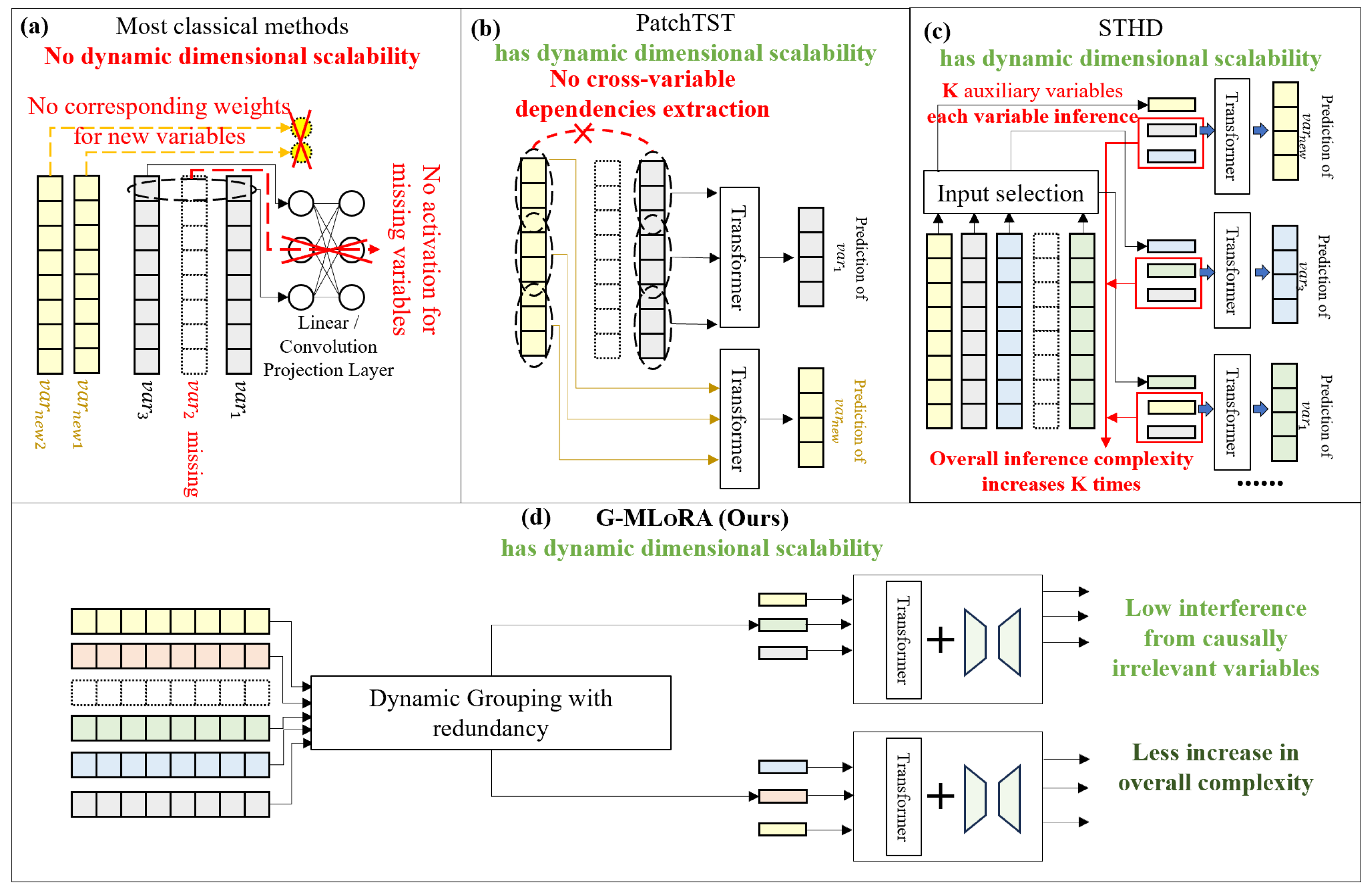
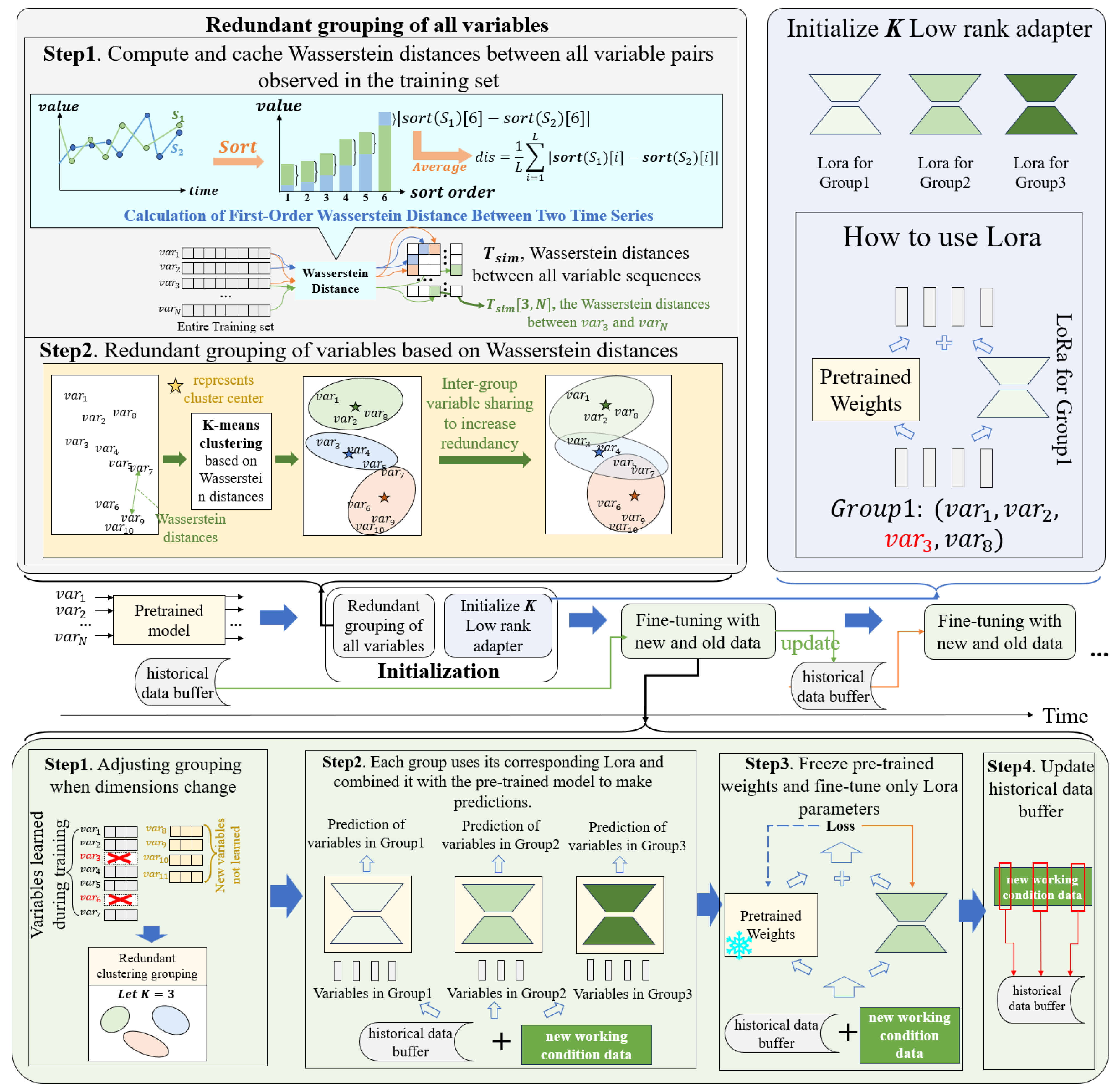
We find that grouping multivariate time series in process industries by inter-variable correlation and then predicting each group separately can significantly improve the robustness of the network against input dimension changes during continual learning. A redundancy clustering method based on Wasserstein distance and K-means is proposed to effectively group multivariate time series with dynamic time delays in inter-variable causal relationships, which implicitly captures the symmetric correlation characteristics among multivariate time series variables and regularizes the feature distribution of dynamic dimensional data.

(2)

Based on the variable grouping strategy, an efficient continual learning method based on multiple low-rank adapters (G-MLoRA) is proposed, in which each variable group is assigned to an exclusive LoRA network. To predict the group, the LoRA network is combined with the pre-trained network, while the pre-trained weights are frozen during each fine-tuning, and only the LoRA network weights are updated. This design realizes symmetric adaptive learning for different variable groups under dynamic dimensional changes, effectively reduces the computational complexity of the continual learning process and mitigates the forgetting of historical knowledge.

(3)

Under a test environment consisting of two real large datasets from grinding and classification processes of different concentrators, extensive comparative and ablation experiments are conducted between the proposed method and the mainstream continual learning methods. Experimental results demonstrate the significant superiority of the proposed method.

2. Methods

2.1. Problem Description

For the continual learning of multivariate time series prediction task in process industries, the objective is defined as follows: consider a multivariate time series system with dynamic dimensions, and denote the observable variable dimension of the system at the $t-th$ continual learning stage (corresponding to a production cycle or data increment batch) as $D_t$ ($D_t$ can change with t, meaning $D_t\ne D_{t-1}$ is possible). Given the historical observation data $X_t^{\mathit{his}} \in R^{L_t \times D_t}$ with $L_t$ consecutive sampling points at this stage, where $X_t^{his}=\left[\begin{array}{cccc}{x}_t^{\left(1,1\right)}& x_t^{\left(1,2\right)}& \cdots & x_t^{\left(1,{\mathrm{D}}_{\mathrm{t}}\right)}\\ x_t^{\left(2,1\right)}& x_t^{\left(2,2\right)}& \cdots & x_t^{\left(2,{\mathrm{D}}_{\mathrm{t}}\right)}\\ \cdots & \cdots & \cdots & \cdots \\ x_t^{({\mathrm{L}}_{\mathrm{t}},1)}& x_t^{({\mathrm{L}}_{\mathrm{t}},2)}& \cdots & x_t^{({\mathrm{L}}_{\mathrm{t}},{\mathrm{D}}_{\mathrm{t}})}\end{array}\right]$, $x_t^{\left(i,d\right)}\in R$ denotes the observed value of the d-th input variable at the i-th time point of the t-th stage. If d is a new variable, there is no data for this variable in the $(t-1)-th$ stage; if d is a removed variable, there is no data for this variable in the t-th stage.

Let the parameters of the model obtained through training with data from the first $(t-1)$ stages be ${\theta }_{t-1}$. When introducing new data from the t-th stage, incremental learning is required to update the model parameters to ${\theta }_t$. The updated model $f\left(\cdot ;{\theta }_t\right)$ should not only predict the system output $X_t^{\mathit{future}}\in R^{H\times D_t}$ for the next H time steps based on the historical data $X_t^{\mathit{his}}$ of the current stage (where $X_t^{future}=\left[\begin{array}{ccc}{x}_t^{\left(L_t+\mathrm{1,1}\right)}& \cdots & x_t^{\left(L_t+1,D_t\right)}\\ \cdots & \cdots & \cdots \\ x_t^{(L_t+H,1)}& \cdots & x_t^{(L_t+H,D_t)}\end{array}\right]$) satisfying $X_t^{\mathit{future}}=f\left(X_t^{\mathit{his}};{\Theta }_t\right)$ but also ensure that the prediction performance of the model on all historical data from previous stages $\{X_1^{\mathit{his}}, X_2^{\mathit{his}},\dots , X_{t-1}^{\mathit{his}}\}$ does not significantly degrade (i.e., mitigating catastrophic forgetting).

2.2. Overview of the Method Architecture

Figure 2 illustrates the basic workflow of classic continual learning for multivariate time series forecasting models, while Figure 3 presents the continual learning process of the proposed G-MLoRA in this paper. The two figures adopt a basically similar framework to facilitate readers’ understanding of the key differences between the method in this paper and the classic method.

G-MLoRA has three main characteristics: (1) Before each inference and fine-tuning, variables are grouped with redundancy (i.e., some variables appear in multiple groups to avoid forced separation of highly correlated variables), and each group is input into the network for prediction separately. This reduces interference from causally irrelevant variables and improves the network’s ability to learn dynamic inter-variable relationships. (2) During continual learning, the backbone network is frozen and only each LoRA network is fine-tuned to reduce computational complexity and mitigate catastrophic forgetting in the compatibility of new and old knowledge. (3) An effective reuse of historical experience with inconsistent dimensions is achieved through mini-batch and gradient accumulation. Since only the weights of LoRA networks are fine-tuned, the proposed method can be directly applied to continual learning of any pre-trained multivariate time series prediction network with dynamic dimensional scalability, represented by iTransformer [27]. Let the parameters of the pre-trained multivariate time series prediction model participating in continual learning be ${\theta }_{base}$, the variable set consisting of all variables in the dataset used for pre-training ${\theta }_{base}$ be $V$, and the number of variable groups be $K$. The overall computational flow of the proposed method is as follows:

(1)

Algorithm Initialization: First, an empty historical data buffer ${Buffer}_{his}\leftarrow \varnothing$ is initialized, and a portion of historical data is randomly selected and added to ${Buffer}_{his}$ for experience replay. Then, using the clustering method described in Section 2.3, variables in $V$ are divided into $K$ groups based on the historical data cached in ${Buffer}_{his}$ using Wasserstein distance and K-means clustering, with some variables assigned to multiple groups simultaneously. Let the i-th group of variables be $G_i$. Next, the parameters of $K$ LoRA networks ${\theta }_{lora}^1,{\theta }_{lora}^2,\dots {\theta }_{lora}^K$ are initialized.

(2)

Inference Process Integrating Multi-LoRA: Let the current multivariate time series to be inferred be $X_{new}\in R^{{S\times L}_{in}\times D_{new}}$, where $S$ is the number of samples, $L_{in}$ is the length of the look-back window, and $D_{new}$ is the number of variables. The variable set consisting of all variables in $X_{new}$ is $V_{new}$. If there are new variables in $V_{new}$ that do not belong to $V$, all new variables are added to $V$, and all variables are redivided into $K$ groups using the method described in Section 2.3. Then, each group of variables is predicted using the backbone network combined with the corresponding LoRA network; that is, the prediction result of the i-th group of variables is ${\overline{Y}}^i=f\left(X_{new} [:,:,\forall var\in G_i];{\theta }_{base}+{\theta }_{lora}^i\right)$. Finally, the prediction results of each group are integrated using the method described in Section 2.4 to obtain the final prediction results for all variables.

(3)

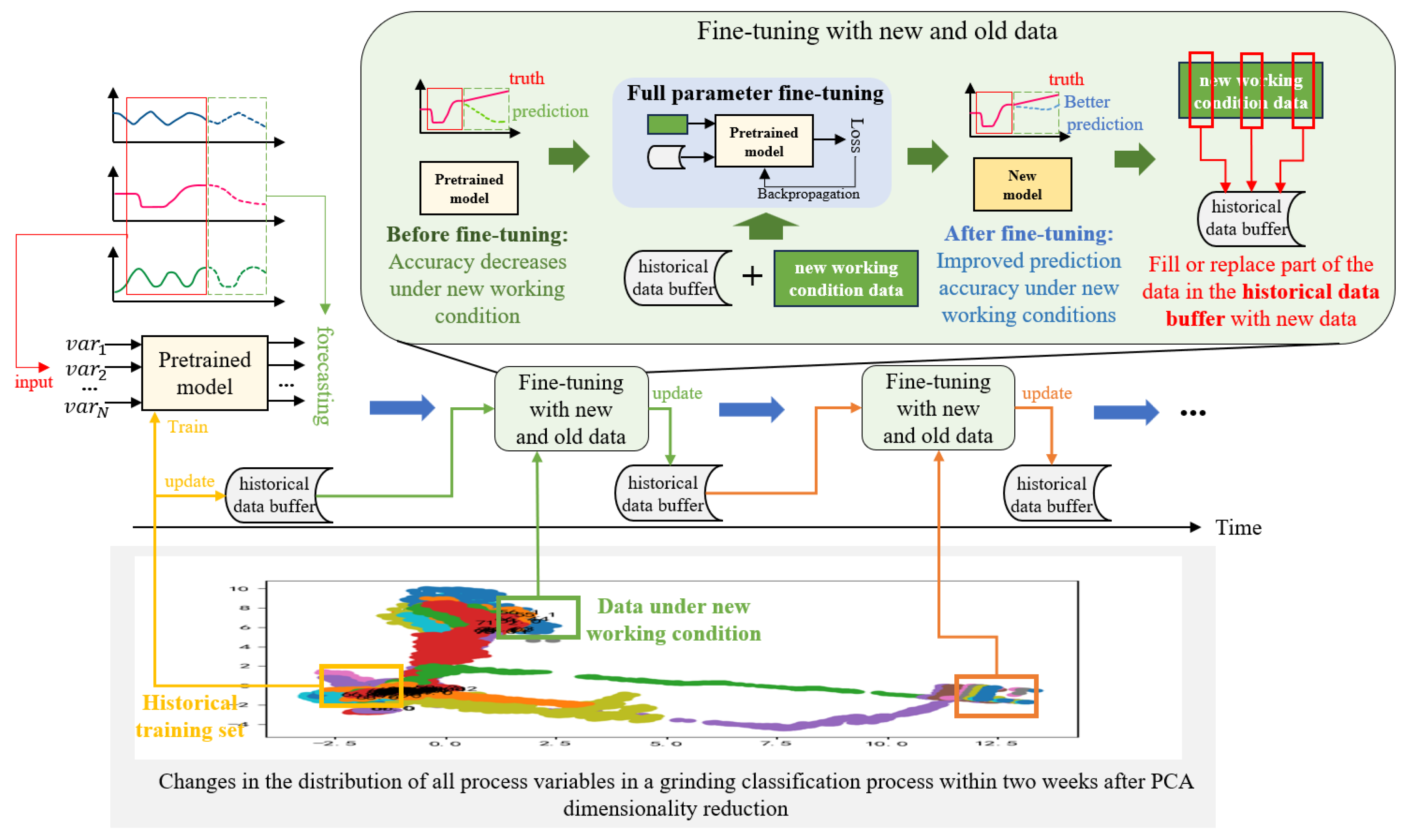
Continual Learning Process of Multi-LoRA: If the continual learning condition is triggered, using the method described in Section 2.5, ${\theta }_{base}$ is first frozen, and then the weights of each LoRA network ${\theta }_{lora}^1,{\theta }_{lora}^2,\dots {\theta }_{lora}^K$ are adjusted separately using gradient descent. After fine-tuning, some new samples are extracted from ${Data}_{new}$ using the reservoir sampling algorithm [33] to replace some old data samples in ${Buffer}_{his}$.

2.3. Redundancy Clustering Method for Multivariate Time Series Based on Wasserstein Distance

Our clustering method consists of two stages. The first stage is the pre-grouping mentioned in Section 2.2 (1), where all variables $V$ encountered during the pre-training of the backbone network are clustered and grouped using the historical data in ${Buffer}_{his}$. The second stage is the dynamic grouping adjustment mentioned in Section 2.2 (2), where grouping is re-adjusted if new variables appear during each inference. The pre-grouping process of the first stage is introduced first.

Pre-Grouping Calculation Process: First, the Wasserstein distance between all variables in $V$ is calculated using the historical data in ${Buffer}_{his}$. Then, the K-means clustering algorithm is used to divide all variables into $K$ groups, where variables with smaller Wasserstein distances are clustered into one group. After grouping, each pair of groups shares 1 variable closest to the cluster center of the other group; i.e., these two variables appear in both groups for input and prediction to avoid forcing highly correlated variables into different groups. The pseudo-code in Algorithm 1 is used to describe the pre-grouping calculation process in detail. For two time series of length $L$, the calculation method of their Wasserstein distance is shown in Equation (1).

$${dis}_{\mathrm{W}\mathrm{a}\mathrm{s}\mathrm{s}\mathrm{e}\mathrm{r}\mathrm{s}\mathrm{t}\mathrm{e}\mathrm{i}\mathrm{n}}(S_1,S_2)={\displaystyle \frac{1}{L}}\sum _{i=1}^L\left|sort\right(S_1) [i]-sort(S_2) [i\left]\right|$$

(1)

Algorithm 1. Time series grouping based on Wasserstein distance and K-means clustering.

Input: $Data\in R^{L\times D}$, the current observable multivariate time series.

Input: $K\in Z^{+}$, the number of groups which the variables are divided into.

Input: $Iter\in Z^{+}$, the number of iterations of K-means algorithm.

Output: $G=\{G_1,G_2,\dots ,G_K\}$, different variable groupings.

# Calculate and cache the Wasserstein distance between all observable variables.

1: $T_{sim}\leftarrow empty\_matrix(shape=D\times D)$

2: for i = 1 to D-1 do:

3:      for j = i to D do:

4:            $T_{\mathit{sim}}[i, j]\leftarrow {\mathit{d}\mathit{i}\mathit{s}}_{\mathbf{W}\mathbf{a}\mathbf{s}\mathbf{s}\mathbf{e}\mathbf{r}\mathbf{s}\mathbf{t}\mathbf{e}\mathbf{i}\mathbf{n}}(Data [:, i], Data [:, j])$

5:            $T_{\mathit{sim}}[j, i]\leftarrow T_{\mathit{sim}}[i, j]$

# Group variables using K-means clustering

6: $C\leftarrow RandomSelect\left(\right\{1,\dots ,D\},GN)$

7: $ClusterIDs\leftarrow Zeros\left(D\right)$

8: for t = 1 to $Iter$ do:

9:        for k = 1 to D do:

10:          $ClusterIDs [k]\leftarrow {argmin}_{i\in C}{T}_{sim} [k,i]$

11:      for m = 1 to K do:

12:          $S_m\leftarrow \{k:ClusterIDs [k]=m\}$

13:          if $S_m\ne \varnothing$ do:

14:             $C [m]\leftarrow {argmin}_{p\in S_m}\sum _{q\in S_m}{T}_{sim} [p,q]$

15: $G\leftarrow \{\varnothing \}\times K$

16: for k = 1 to $D$ do:

17:      $G [ClusterIDs [k]]\leftarrow G [ClusterIDs [k]]\cup \left\{k\right\}$

# Each two groups share 2 closest variables.

18: for i = 1 to $K$ do:

19:      for j = 1 to $K$ do:

20:          if $i\ne j$ do:

21:             ${center}_i\leftarrow C [i]$

22:             ${center}_i\leftarrow C [j]$

23:              ${dist}_{i,j} \leftarrow \{ T_{sim} [v, center\_j] | v \in G [i] \}$

# Group i selects a variable closest to group j

24:             ${sorted}_{{vars}_i}\leftarrow \mathit{S}\mathit{o}\mathit{r}\mathit{t}(G [i], key=lambda v:{dist}_{i,j} [v])$

25:             ${shared\_var}_i \leftarrow {sorted}_{{vars}_i} [0]$

26:             ${sorted}_{{vars}_i}\leftarrow \mathit{S}\mathit{o}\mathit{r}\mathit{t}(G [i], key=lambda v:{dist}_{i,j} [v])$

27:             ${shared\_var}_i \leftarrow {sorted}_{{vars}_i} [0]$

# Group j selects a variable closest to group i

28:             ${sorted}_{{vars}_j}\leftarrow \mathit{S}\mathit{o}\mathit{r}\mathit{t}(G [j], key=lambda v:{dist}_{i,j} [v])$

29:             ${shared\_var}_j \leftarrow {sorted}_{{vars}_j} [0]$

30:             ${sorted}_{{vars}_i}\leftarrow \mathit{S}\mathit{o}\mathit{r}\mathit{t}(G [i], key=lambda v:{dist}_{i,j} [v])$

31:             ${shared\_var}_j \leftarrow {sorted}_{{vars}_j} [0]$

# share variables

32:             $G [j] \leftarrow G [j] \cup {shared\_var}_i$

33:             $G [i] \leftarrow G [i] \cup {shared\_var}_j$

34: return $G$

Dynamic grouping adjustment calculation process: If no new variables appear in the data to be inferred $X_{new}\in R^{L_{in}\times D_{new}}$ but only some previously learned variables are missing, that is, $D_{new}<\left|V\right|$ and $\forall v\in X_{new}, v\in V$, the grouping will not be adjusted. However, if there are new variables in $X_{new}$ that are not in $V$, that is, $\exists v\in X_{new}, v\notin V$, the Wasserstein distance between the new variables and other learned variables is calculated based on the sequences in $X_{new}$, and the new variables are assigned to the group corresponding to the learned variables included in $X_{new}$ that are closest to them.

We choose Wasserstein distance over Pearson correlation coefficient and mutual information for correlation analysis of multivariate time series in process industries. Process industrial systems involve spatial equipment distribution and material transfer, leading to dynamic time lags between variables and strong non-linear correlations. Pearson correlation only captures linear, simultaneous relationships, failing to account for time-shifted dependencies and becoming misleading in asynchronous interactions. Mutual information, while sensitive to non-linearity, relies on distribution estimation and underestimates correlations when lags are variable or unknown. In contrast, Wasserstein distance quantifies overall distributional similarity, inherently accommodating dynamic lags without requiring time synchronization. It also captures non-linear dependencies effectively without explicit modeling, providing a more reliable measure of intrinsic correlations in process industrial time series.

2.4. Multivariate Time Series Forecasting Process Based on Redundancy Clustering and Multiple Low-Rank Adapters

As analyzed in the introduction, the core challenge of multivariate time series prediction in process industries is to continuously learn complex inter-variable relationships under scenarios where inter-variable relationships and dimensions are both dynamically changing and effectively utilize new and old knowledge with inconsistent dimensions to avoid catastrophic forgetting affecting generalization ability. The inference method proposed in this section, based on the redundant variable grouping results obtained in Section 2.3, achieves robust handling of dimension changes through a two-step strategy of “group-independent inference + result integration”. The specific process is as follows.

2.4.1. Variable Group Matching Before Inference

Let the variable grouping set obtained through redundant clustering in Section 2.3 be $G=\{G_1,G_2,\dots ,G_K\}$, where $G_i$ denotes the i-th variable group, satisfying ${\bigcup }_{i=1}^K{G}_i=V$ ($V$ is the set of all variables up to the current time) and allowing inter-group variable redundancy (i.e., $\exists i\ne j$ such that $G_i\cap G_j\ne \varnothing$).

For the current multivariate time series data to be inferred $X_{\mathit{new}}\in R^{S\times L_{\mathit{in}}\times D_{\mathit{new}}}$ (S is the number of samples, $L_{\mathit{in}}$ is the input time window length, $D_{\mathit{new}}$ is the variable dimension of the current data), the variable set it contains $V_{\mathit{new}}\subseteq V$ is first extracted. For each variable group $G_i$, the variable subset belonging to $G_i$ in $X_{\mathit{new}}$ is filtered to form the input data of the group $X_{\mathit{new}}^{\left(i\right)}$; that is,

$$X_{\mathit{new}}^{\left(i\right)}= X_{\mathit{new}}\left[:,:,\forall \mathit{var}\in G_i \cap V_{\mathit{new}}\right]$$

(2)

If $X_{\mathit{new}}$ lacks some variables in $G_i$, no interpolation or completion operation is required, and only the existing variable dimensions are retained. At this time, the dimension of $X_{\mathit{new}}^{\left(i\right)}$ is $R^{S\times L_{\mathit{in}}\times D_i^{\prime }}$ ($D_i^{\prime }\le \left|G_i\right|$, $\left|G_i\right|$ is the total number of variables in $G_i$).

2.4.2. Group-Independent Inference

To reduce interference from causally irrelevant variables and improve the learning effect of inter-variable dependencies, the inference process of each variable group $G_i$ adopts a fusion mode of “Backbone weights + exclusive LoRA weights”. Let the parameters of the pre-trained backbone network be ${\theta }_{\mathit{base}}$, and the parameters of the i-th LoRA network be ${\theta }_{\mathit{lora}}^i$ (in the form of a low-rank matrix, satisfying ${\theta }_{\mathit{lora}}^i= A^i\cdot {\left(B^i\right)}^T$, where $A^i\in R^{d\times r}$, $B^i\in R^{d\times r}$, d is the dimension of the corresponding layer of the backbone, and r is the low-rank dimension). The fusion weights of the i-th group are

$${\theta }_{\mathit{fusion}}^i= {\theta }_{\mathit{base}}+ {\theta }_{\mathit{lora}}^i$$

(3)

Input $X_{\mathit{new}}^{\left(i\right)}$ into the network based on ${\theta }_{\mathit{fusion}}^i$ to obtain the prediction result $Y^{\left(i\right)}$ of the i-th group. Let the prediction function of the network be $f\left(\cdot ; \theta \right)$ (including feature extraction, temporal modeling, and output mapping), then

$$Y^{\left(i\right)}=f\left(X_{\mathit{new}}^{\left(i\right)}; {\theta }_{\mathit{fusion}}^i\right)$$

(4)

where $Y^{\left(i\right)}\in R^{S\times L_{\mathrm{out}}}$, $L_{\mathrm{out}}$ is the prediction time window length, and the predicted variables of $Y^{\left(i\right)}$ are the variables in $G_i$.

2.4.3. Integration of Multi-Group Prediction Results

Due to inter-group variable redundancy, prediction results of different groups may overlap and cover the same target variable. An integration strategy is needed to fuse multi-group information to improve prediction accuracy. This paper adopts an average integration method, and determines integration rules according to the number of occurrences of variables in each group (single-group occurrence/multi-group occurrence). The specific steps are as follows:

(1)

Statistics of variable occurrence times: let the set of target prediction variables be $Y_{\mathit{tar}}$ (in one-to-one correspondence with $V_{\mathit{new}}$). For each target variable $y_t\in Y_{\mathit{tar}}$, count the set of variable groups containing $y_t$, $G_{y_t}=\left\{G_i\right|y_t\in G_i\}$, and calculate the set size $\left|G_{y_t}\right|$ (i.e., the number of groups containing $y_t$).

(2)

Result processing for variables appearing in a single group: if $\left|G_{y_t}\right|=1$ (i.e., $y_t$ appears only in the unique group $G_i$), the prediction result of this group for $y_t$ is directly used as the intermediate result. At this time, the intermediate prediction value ${\widehat{y}}_{t,\mathrm{mid}}$ of $y_t$ satisfies

$${\widehat{y}}_{t,\mathrm{mid}}=Y^{\left(i\right)}\left(:,:,t^{\prime }\right)$$

(5)

where $G_i$ is the only group containing $y_t$, and $t\prime$ is the dimension index of $y_t$ in $Y^{\left(i\right)}$.

Result processing for variables appearing in multiple groups: if $\left|G_{y_t}\right|\ge 2$ (i.e., $y_t$ appears in multiple groups), the mean of the prediction results of all groups containing $y_t$ for $y_t$ is used as the intermediate result. At this time, the intermediate prediction value ${\widehat{y}}_{t,\mathrm{mid}}$ of $y_t$ satisfies

$${\widehat{y}}_{t,\mathit{mid}}={\displaystyle \frac{1}{\left|G_{y_t}\right|}}\sum _{G_i\in G_{y_t}}{Y}^{\left(i\right)}\left(:,:,t_i^{\prime }\right)$$

(6)

where $t_i^{\prime }$ is the dimension index of $y_t$ in the prediction result $Y^{\left(i\right)}$ of the i-th group, and $\left|G_{y_t}\right|$ is the number of groups containing $y_t$ (e.g., if $y_t$ is included in 4 groups, $\left|G_{y_t}\right|=4$, i.e., the prediction values of the 4 groups are summed and divided by 4).

Integration of final prediction results: integrate the intermediate prediction values ${\widehat{y}}_{t,\mathit{mid}}$ of all target variables according to the variable order of $Y_{\mathit{tar}}$ to obtain the final prediction matrix $Y_{\mathit{final}}\in R^{S\times L_{\mathit{out}}\times D_{\mathit{new}}}$. Its mathematical expression is

$$Y_{\mathit{final}}\left[:,:,t\right]=\left\{\begin{array}{cc}{Y}^{\left(i\right)}\left(:,:,t\right)& , \left|G_{y_t}\right|=1\\ {\displaystyle \frac{1}{\left|G_{y_t}\right|}}{\displaystyle \sum _{G_i\in G_{y_t}}{Y}^{\left(i\right)}\left(:,:,t_i^{\prime }\right)}& , \left|G_{y_t}\right|\ge 2\end{array}\right.$$

(7)

2.5. Multi-LoRA Network Continual Learning Method Based on Mini-Batch Gradient Accumulation

Study [13] has shown that including both new and old data in each batch when triggering continual learning can lead the network weights to optimize in a direction that balances new and old knowledge. However, in dynamic dimension scenarios, there may be inconsistencies in the dimensions of new and old data. The mini-batch gradient accumulation method proposed in this section solves the above problem through a strategy of “gradient accumulation + unified parameter update”. The specific process is as follows:

2.5.1. Training Data Preprocessing and Grouping

When continual learning is triggered, the available training data set is $D_{\mathit{train}}={\mathit{Buffer}}_{\mathit{his}}\cup {\mathit{Data}}_{\mathit{new}}$, where the historical sample dimensions in ${\mathit{Buffer}}_{\mathit{his}}$ are $D_{\mathrm{his}}^m$, the sample dimension of ${\mathit{Data}}_{\mathit{new}}$ is $D_{\mathit{new}}$, and ${\bigcup }_{m=1}^M{D}_{\mathit{his}}^m\cup D_{\mathit{new}}\subseteq V$.

First, based on the latest variable grouping results $G=\{G_1,G_2,\dots ,G_K\}$ in Section 2.3, all samples in $D_{\mathrm{train}}$ are split by group to obtain the corresponding training subset for each group $D_{\mathit{train}}=\{X [:,:,\forall \mathit{var}\in G_i\left]\right|X\in D_{\mathit{train}}\}$ ($i=1,2,\dots ,K$).

For each $D_{\mathit{train}}^{\left(i\right)}$, it is further divided according to the number of variable dimensions of the samples to obtain several mini-batch subsets with the same dimension. Let the dimension set of samples in $D_{\mathit{train}}^{\left(i\right)}$ be $\{d_{i,1},d_{i,2},\dots ,d_{i,T}\}$ ($d_{i,t}\le \left|G_i\right|$), then the mini-batch of the corresponding dimension $d_{i,t}$ is

$$B_{i,t}=\left\{X^{\left(i\right)}\in D_{\mathit{train}}^{\left(i\right)}∣\mathit{dim}\left(X^{\left(i\right)}\right)=d_{i,t}\right\}$$

(8)

where $\dim \left(X^{\left(i\right)}\right)$ denotes the variable dimension of $X^{\left(i\right)}$.

2.5.2. Gradient Accumulation and Parameter Update Strategy

To ensure the stability of parameter updates, a strategy of “multi-mini-batch gradient accumulation—single parameter update” is adopted for each LoRA network ${\theta }_{\mathit{lora}}^i$. During the entire process, the backbone network parameters are frozen, and only the LoRA parameters are updated. The specific steps are as follows:

(1)

Loss function definition: Let the prediction loss of the i-th group be the Mean Squared Error (MSE) loss, which is used to measure the deviation between the predicted value and the true value. For the sample $\left(X^{\left(i\right)}, Y_{\mathit{gt}}^{\left(i\right)}\right)$ in mini-batch $B_{i,t}$ ($Y_{\mathit{gt}}^{\left(i\right)}$ is the true label), its loss is

$$L_{i,t}={\displaystyle \frac{1}{B\cdot L_{\mathit{out}}}}\sum _{ X^{\left(i\right)}\in B_{i,t}}|f\left(X^{\left(i\right)}; {\theta }_{\mathit{base}}+ {\theta }_{\mathit{lora}}^i\right) - Y_{\mathit{gt}}^{\left(i\right)}{|}_2^2$$

(9)

(2)

Gradient calculation and accumulation: for each $B_{i,t}$, calculate the gradient ${\nabla }_{{\mathsf{\theta }}_{\mathrm{lora}}^i}{L}_{i,t}$ of the loss $L_{i,t}$ with respect to ${\theta }_{\mathit{lora}}^i$, and accumulate it into the gradient buffer variable ${\nabla }_{\mathrm{acc}}^i$. Let the i-th group have $T_i$ mini-batches with the same dimension, then the gradient accumulation process is

$${\mathsf{\nabla }}_{\mathit{acc}}^i=\sum _{t=1}^{T_i}{\mathsf{\nabla }}_{{\theta }_{\mathit{lora}}^i}{L}_{i,t}$$

(10)

Among them, the gradient calculation adopts the backpropagation algorithm, and the gradient calculation processes of different mini-batches are independent of each other to avoid gradient interference from samples with inconsistent dimensions.

Unified parameter update: after the gradient accumulation of all mini-batches in the i-th group is completed, the gradient descent is used to update ${\theta }_{\mathit{lora}}^i$. Let the learning rate be $\mathsf{\eta }$; then, the parameter update formula is

$${\theta }_{\mathit{lora}}^i\leftarrow {\theta }_{\mathit{lora}}^i-\eta \cdot {\displaystyle \frac{{\mathsf{\nabla }}_{\mathit{acc}}^i}{T_i}}$$

(11)

Dividing by $T_i$ normalizes the accumulated gradient to ensure that the actual step size of the learning rate matches the mini-batch size, avoiding parameter oscillation caused by excessive gradient magnitude.

2.5.3. ${Buffer}_{his}$ Update Method Based on Reservoir Sampling

To ensure the timeliness and representativeness of the historical data in ${Buffer}_{his}$, after the parameter update of the multi-LoRA network is completed, the reservoir sampling algorithm [33] is adopted to update ${Buffer}_{his}$, with the specific rules as follows:

(1)

Let the fixed capacity of ${Buffer}_{his}$ be $C$, the number of samples to be replaced be $P$ ($P \le C$), and the total number of samples in ${\mathit{Data}}_{\mathit{new}}$ be $S$.

(2)

Initialize the reservoir ${Buffer}_{his}$. If $\left|{Buffer}_{his}\right| < C$, first fill the samples in ${\mathit{Data}}_{\mathit{new}}$ into ${Buffer}_{his}$ until it reaches full capacity; if |${Buffer}_{his}$| = C, for each new sample $X_{\mathit{new}}$∈ ${\mathit{Data}}_{\mathit{new}}$, generate a random number $r \in [0,1)$. If $r<{\displaystyle \frac{P}{N}}$, randomly replace an old sample in ${Buffer}_{his}$.

3. Experiments and Discussion

The experimental part mainly discusses six areas, and all experimental verification in this paper was carried out for the grinding and classification process, a typical industrial process:

(1)

In the continual learning process with a fixed number of variables (i.e., the idealized scenario targeted by most classic continual learning methods), the error change of G-MLoRA and classic learning methods on new data and the forgetting of historical knowledge;

(2)

In the continual learning process with dynamic changes in the number of variables (i.e., a scenario often encountered in practical industrial applications), the comparison of historical knowledge forgetting between G-MLoRA and classic learning methods;

(3)

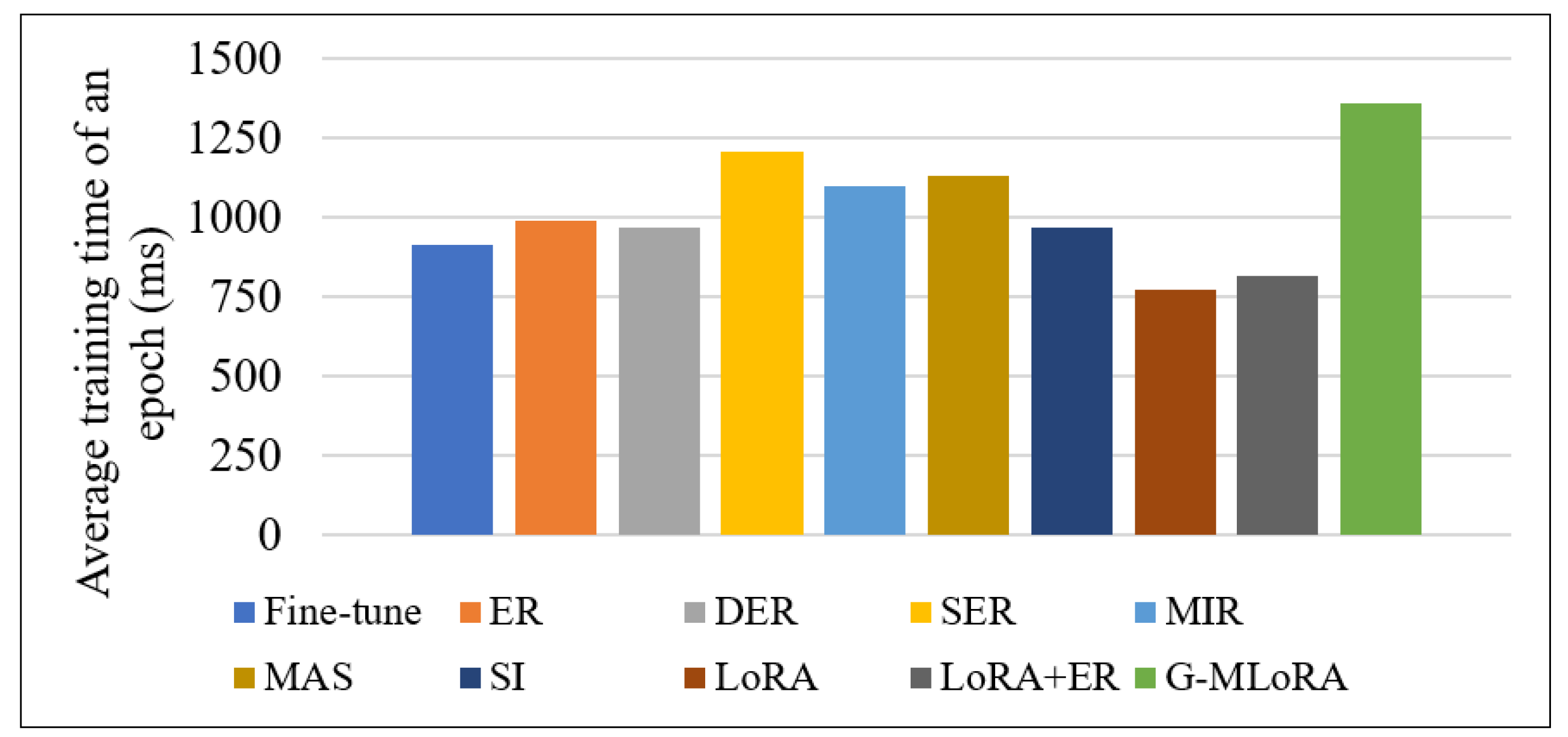
Comparison of computational efficiency between G-MLoRA and classic methods;

(4)

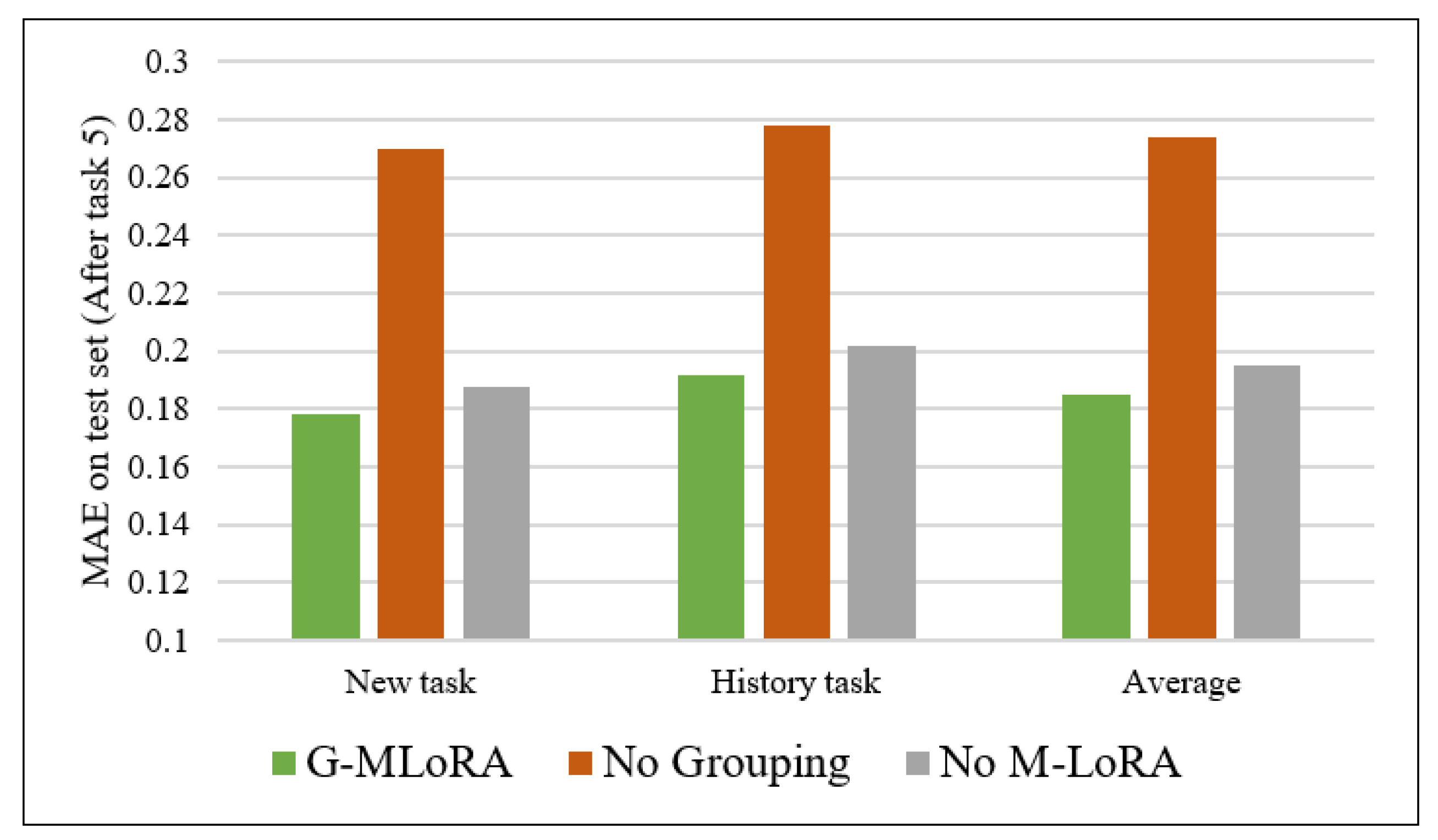
Ablation experiments, mainly comparing the impact of removing the variable grouping strategy and LoRA fine-tuning;

(5)

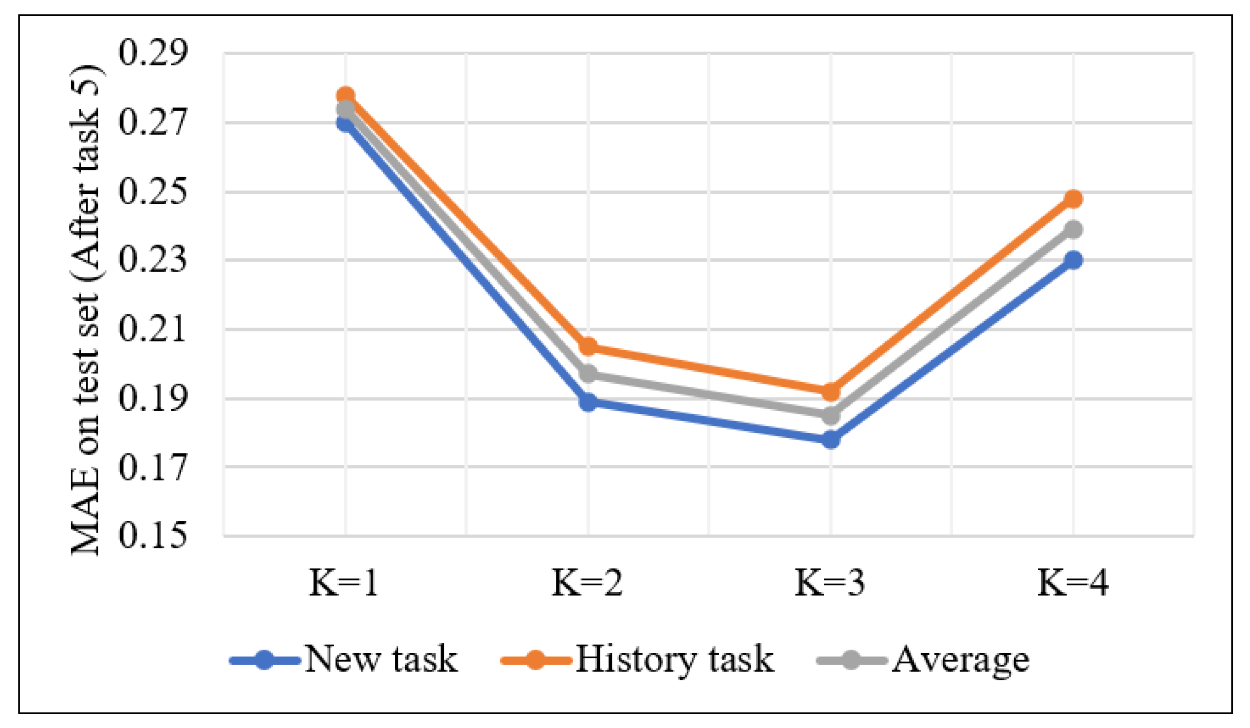
Hyperparameter impact experiments, mainly comparing the impact of changing the number of variable groups.

The details of the datasets used in the experiments are introduced in Section 3.1, and the compared continual learning baselines and error metrics are introduced in Section 3.2.

3.1. Dataset Introduction

We utilized 2 datasets collected from 2 different grinding classification processes. The variables contained in these datasets are detailed in

Table 1. Detail information of dataset A. The symbol # in the variable name represents a delimiter, which is used to distinguish different sampling points of the same variable.

Variables	Dataset Size
Belt conveyor·1
Water flow·SAG
Power·SAG
Belt conveyor·2
Slurry pool level 1
Cyclone pressure 1#1
Cyclone feed concentration·1#1	40,000 points
Cyclone feed flow 1
Cyclone pressure 2#1
Cyclone feed flow 2
Sound of ball mill
SAG sound current 1
Ball mill sound current 2
Cyclone overflow concentration
Particle overflow size

and

Table 2. Detail information of dataset B.

Variables	Dataset Size
Cyclone Inlet Pressure 1 Left Pipe
Cyclone Inlet Pressure 1 Right Pipe
Sound Ball Mill 1
Water Flow Ball Mill Inlet 1
Water Flow Slurry Pool 1 Makeup
Flow 1 Left Pipe
Concentration 1 Left Pipe
Flow 1 Right Pipe
Concentration 1 Right Pipe	28,000
Flow Cyclone Output 1
Concentration Cyclone Output 1
Level Slurry Pool 1
Cyclone Inlet Pressure 2 Right Pipe
Cyclone Inlet Pressure 2 Left Pipe
Flow 2 Left Pipe
Concentration 2 Left Pipe
Flow 2 Right Pipe
Concentration 2 Right Pipe
Flow Cyclone Output 2
Level Slurry Pool 2

. To fully verify the robustness and computational efficiency of the proposed method, the neural network constructed in this experiment will predict all variables in Table 1 and Table 2. However, in practical applications, the proposed method can be flexibly adapted to specific industrial time series prediction or soft measurement tasks with many-to-many or many-to-one relationships by simply modifying the output layer dimension.

(1)

Dataset A: Multivariate time series dataset for a two-stage grinding classification process at beneficiation plant A.

In this plant, the raw ore is first sent into a semi-autogenous grinding (SAG) mill by a belt conveyor, where it is ground with water added at the mill inlet. The output slurry is transferred to a slurry pool and then fed into a cyclone classifier via a slurry pump for classification. The fine-grained overflow from the classifier proceeds to the subsequent flotation stage, while the coarse-grained material settles into a ball mill for further grinding. The slurry from the ball mill is also transferred back into the pump pool. The variables included in dataset A are detailed in Table 1, with a sampling frequency of one data point per minute.

(2)

Dataset B: Multivariate time series dataset for the two-stage ball mill grinding classification process at beneficiation Plant B.

In this plant, the raw ore is first sent into the primary ball mill, where it is ground with the addition of water. The output slurry flows into a Slurry Pool 1 and is then fed into a cyclone classifier via a slurry pump for classification. The fine-grained overflow of the classifier is transferred to Slurry Pool 2, while the coarse-grained material settles back into the primary ball mill for regrinding. In Slurry Pool 2, the slurry is pumped into a secondary cyclone for further classification. The fine-grained overflow proceeds to the flotation stage, while the coarse-grained material settles into the secondary ball mill for regrinding. The slurry output from the secondary ball mill flows into Slurry Pool 2. The variables contained in the dataset are detailed in Table 2, with a sampling frequency of one data point per minute.

3.2. Introduction to Compared Continual Learning Baselines and Comparison Modes

Compared Baselines: In the experimental part, iTransformer [27] is adopted as the backbone prediction network. The compared continual learning baseline methods can be divided into four categories according to their characteristics: (1) Continual learning methods based on experience replay: ER [5], DER [7], MIR [12], CLS-ER [10], SER [9]. (2) Continual learning methods based on regularization: MAS [15], SI [14]. These two methods were verified based on image classification tasks in the original papers, so the cross-entropy loss term in their learning objectives is replaced with MSE loss in the implementation. (3) Continual learning methods based on adapter: LoRA fine-tuning [21], LoRA fine-tuning + ER. (4) Ordinary fine-tuning, i.e., full-parameter fine-tuning of the backbone network only on new data. The main hyperparameter settings of these baseline methods are shown in

Table 3. Detail information of baseline hyperparameters.

Method	Hyperparameter Value
ER	Buffer_size = 1000, α = 0.2
DER	Buffer_size = 1000, α = 0.2, β = 0.2
MIR	Buffer_size = 1000, temporary_buffer_size = 50, α = 0.2
MAS	$\lambda =0.2$, $\gamma =1, loss=\mathrm{M}\mathrm{S}\mathrm{E}$
SI	$\lambda =0.2$, $\gamma =1, loss=\mathrm{M}\mathrm{S}\mathrm{E}$
CLS-ER	$r_p=0.3$, $r_S=0.1$, ${\alpha }_P=0.1$, ${\alpha }_S=0.2$
SER	Buffer_size = 1000, α = 0.2, β = 0.2, $\gamma =0.2$
LoRA/LoRA+ER/Ours	Buffer_size = 1000, r = 8, k = 3

. The hyperparameter values listed in Table 3 were first determined with reference to Study [11], which also compared the continual learning performance of the above baselines on a time series forecasting task for the grinding classification process, with the same application background and learning paradigm as those adopted in this paper. In addition, before conducting the formal experiments, we globally adjusted the hyperparameters from Study [11] (both increasing and decreasing them as a whole) and compared their performance on the first round of the continual learning task using Dataset A. The results demonstrate that the current hyperparameters presented in Table 3 achieve relatively superior performance. The insertion positions of LoRA weights are the projection layers of query, key, value of each layer, and the final output layer.

Continual learning performance comparison mode and compared metrics: the characteristic of continual learning tasks is that the model will continuously encounter data under new operating conditions. After training on new data, it should not only effectively reduce the prediction error under new operating conditions but also not lose too much historical knowledge. Therefore, we adopt a method of first pre-training a model and then fine-tuning the model with new operating condition data at intervals to simulate the continual learning scenario commonly encountered in practical industrial applications and observe the error changes of the model on new and old data during this process. The specific comparison method is as follows:

(1)

Assume there are 10,000 time steps of data in the dataset. According to the time sequence, the first 3000 time steps of data (the first 30%) are taken from the dataset without replacement. Among them, the first 2100 time steps (the first 70%) are used as the training set to train a pre-trained time series prediction model, and the last 900 time steps of data are used as the test set for the pre-training process to participate in the subsequent test of historical knowledge forgetting degree.

(2)

Then, each time, the first 1400 time steps of data are taken from the remaining data without replacement (i.e., the remaining 70% of the data not participating in pre-training is equally divided into 5 parts, called 5 tasks, each task accounting for 14% of the total original data) (simulating the model encountering a new operating condition prediction task). Among them, the first 1000 time steps of data are used as the training set for this fine-tuning, and the last 400 time steps of data are used as the test set for this fine-tuning.

(3)

At this time, different continual learning methods are used to adjust the model weights, and two types of metrics are compared, respectively: (1) New data error, i.e., the prediction error on the test set of the current task. We call this error the new data error. The lower the new data error, the better the ability of the corresponding method to adapt to new knowledge. (2) Historical data error, i.e., the prediction error of the network on the test sets of previous rounds after learning the training set of the current round of tasks. The lower the historical data error, the stronger the ability of the corresponding method to retain historical knowledge during continual learning.

3.3. Comparison of New and Old Knowledge Error Changes of Different Methods in Continual Learning with Fixed Number of Variables

This experiment compares the performance differences between the proposed G-MLoRA method and mainstream continual learning methods under the classic idealized scenario with a fixed number of variables. The experiment is carried out in the “pre-training + 5 new tasks” mode proposed in Section 3.2. The specific hyperparameter settings are as follows:

(1)

Data Processing: All datasets are standardized using Z-score. The input time window length (look-back window) is uniformly set to 48 (corresponding to 48 min of historical data), and the prediction length is uniformly set to 24.

(2)

Model Parameters: The backbone network selects iTransformer [27], the hidden layer dimension is set to 256, the number of attention heads is 2, and the number of encoder layers is 2; the low-rank dimension r of G-MLoRA is 8, the number of groups K is 3, and the insertion positions of LoRA adapters are the Q/K/V projection layers of each encoder layer and output layer.

(3)

Training Parameters: All methods adopt the Adam optimizer with an initial learning rate of 0.0001. The batch size for pre-training and subsequent continual learning is set to 32. The training epoch for pre-training is 10, and the training epoch for each fine-tuning is 3. The loss function uniformly uses Mean Squared Error (MSE). The experimental environment consists of an Intel 13700K CPU and an NVIDIA 3090TI GPU. For the software components, the operating system is Windows 11, the Python version is 3.9.20, and the PyTorch version is 2.8.0.

The experimental results on datasets A and B are shown in Figure 4 and Figure 5, respectively. The horizontal axis numbers in Figure 5 and Figure 6 represent the i-th time continual learning is triggered (or the i-th batch of new operating condition data is encountered). Different curves represent the error changes of different continual learning methods on the new and old data test sets as the number of rounds increases. The comprehensive performance comparison of the error conditions on the two datasets is shown in Figure 6.

Analyzing the experimental results, the following key phenomena can be found:

(1)

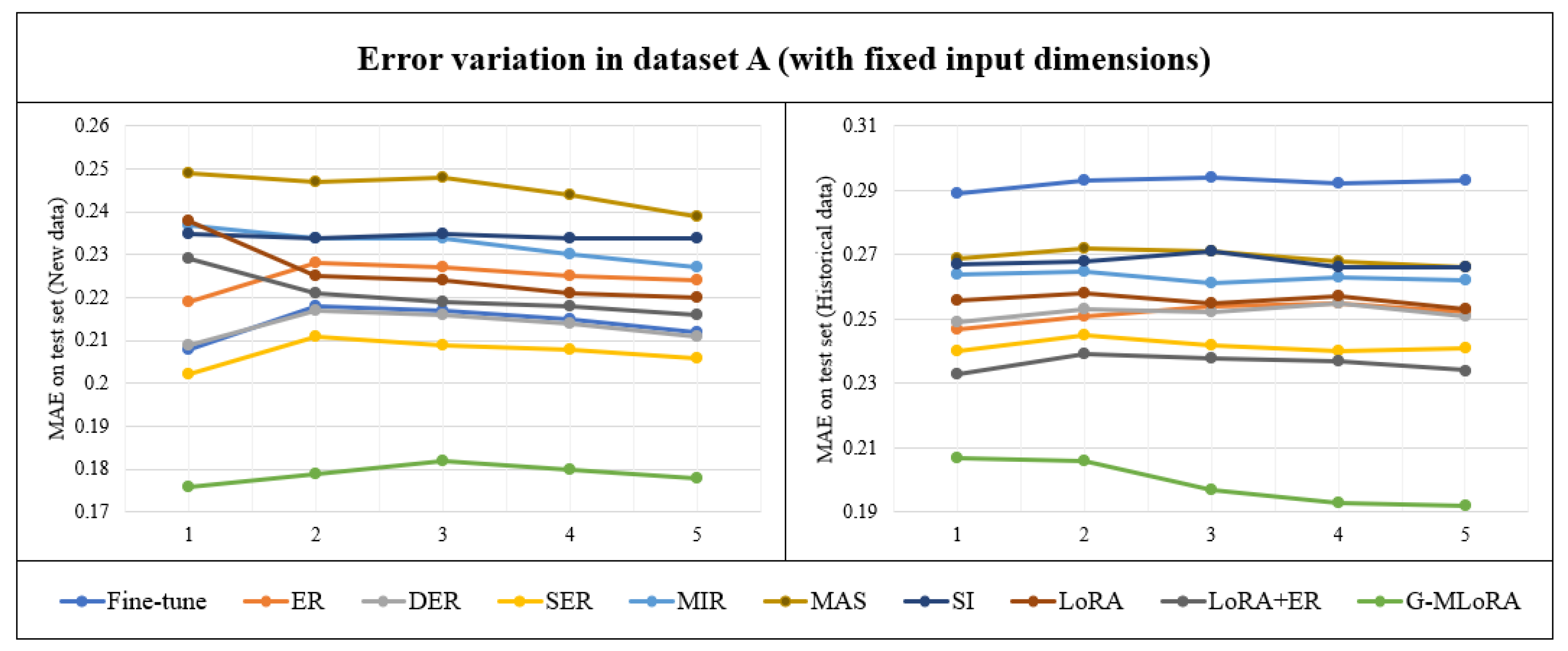
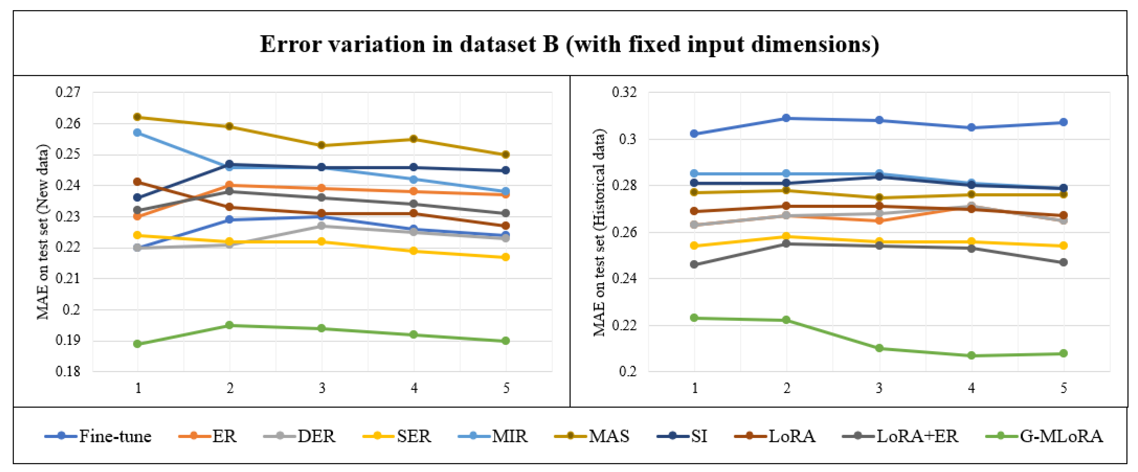
Figure 4 and Figure 5 show that the ordinary fine-tuning method based on fine-tuning only on new data has significantly worse historical knowledge retention ability than other continual learning methods, and its adaptation speed to new knowledge is not better than other continual learning methods in most cases. We believe this is partly because the grinding and classification process is a typical slow-varying system, and there is no lack of guidance between new knowledge and historical knowledge. Therefore, integrating part of historical knowledge in the continual learning of such slow-varying systems can not only avoid catastrophic forgetting but also improve the learning effect of new knowledge to a certain extent.

(2)

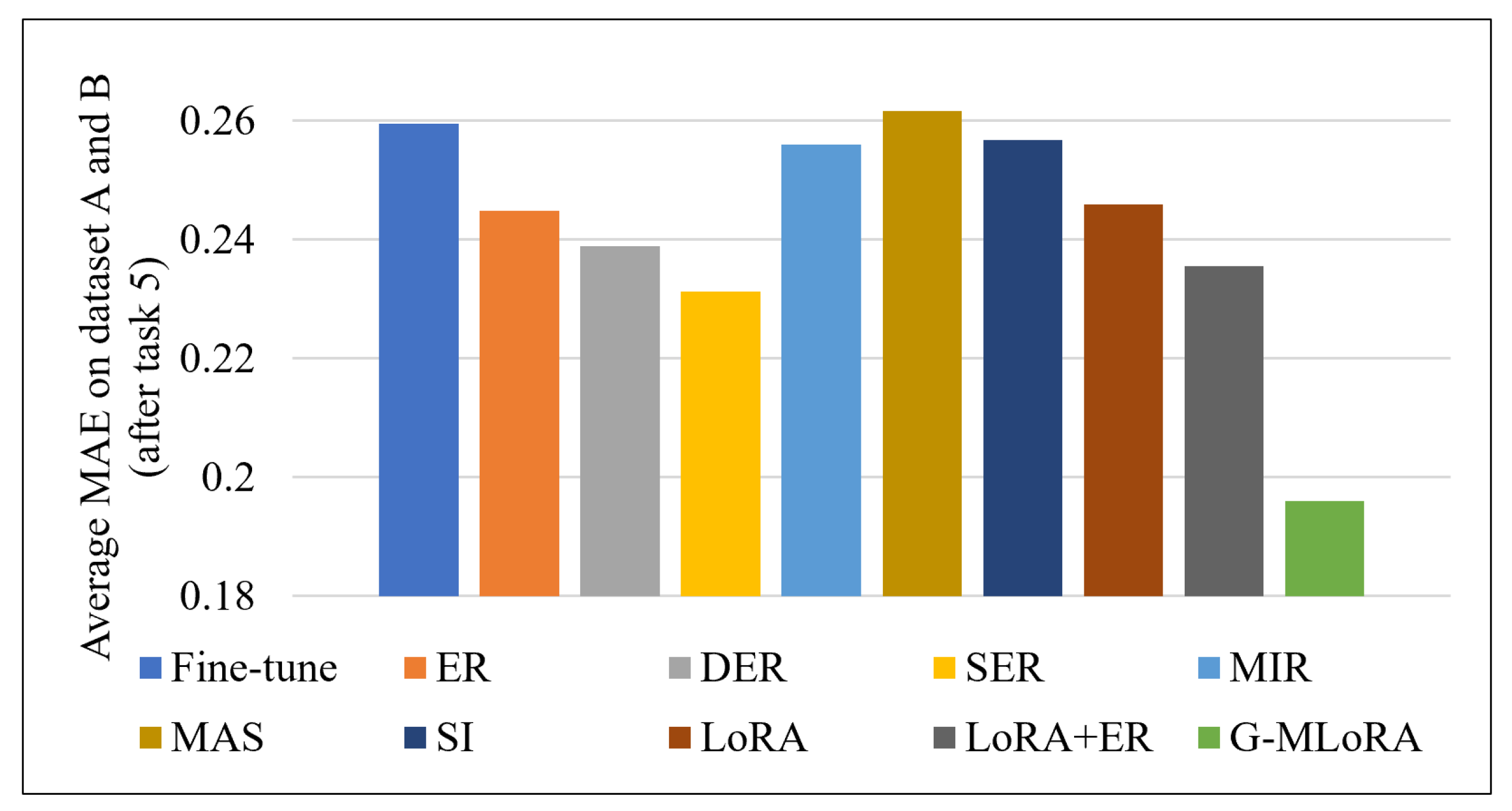
From the comprehensive results in Figure 6, compared with experience replay methods that replay historical samples, the fine-tuning methods based only on regularization or fine-tuning only on new data have relatively higher errors. This indicates that in the design of continual learning methods for multivariate time series in process industries represented by grinding and classification processes, retaining direct historical sample replay or historical hidden feature replay is quite important and even necessary under current technical conditions.

(3)

In all cases, the continual learning error of G-MLoRA on new and old data is the lowest and significantly lower than the LoRA+ER method, which also adopts adapter and experience replay. This indicates that even in the traditional ideal scenario with fixed variable dimensions, the grouping strategy proposed in this paper can still bring significant performance improvements. We believe this shows the effectiveness and importance of introducing the variable grouping strategy to reduce the proportion of redundant information in systems with highly dynamic and inconsistent inter-variable relationships such as process industries.

3.4. Comparison of New and Old Knowledge Error Changes of Different Methods in Continual Learning with Dynamic Changes in the Number of Variables

This experiment simulates the dynamic dimension change of “variable addition or missing” in practical industrial application scenarios. First, in the pre-training stage, only ${\displaystyle \frac{2}{3}}$ of the variables in the dataset are used for pre-training (for dataset A, 10 variables are used to train the initial prediction model; for dataset B, 13 variables are used to train the initial prediction model). Then, in the 2nd and 4th rounds of the subsequent 5 rounds of fine-tuning, 1~2 variables are randomly selected from the variables not participating in pre-training and added to the new data. In the 1st, 3rd, and 5th rounds of fine-tuning, 1~2 variables learned in the pre-training stage are randomly removed in the new data. The continual learning performance of G-MLoRA and baseline methods under dynamic dimension changes is compared. The experimental settings are adjusted based on Section 3.3 as follows:

(1)

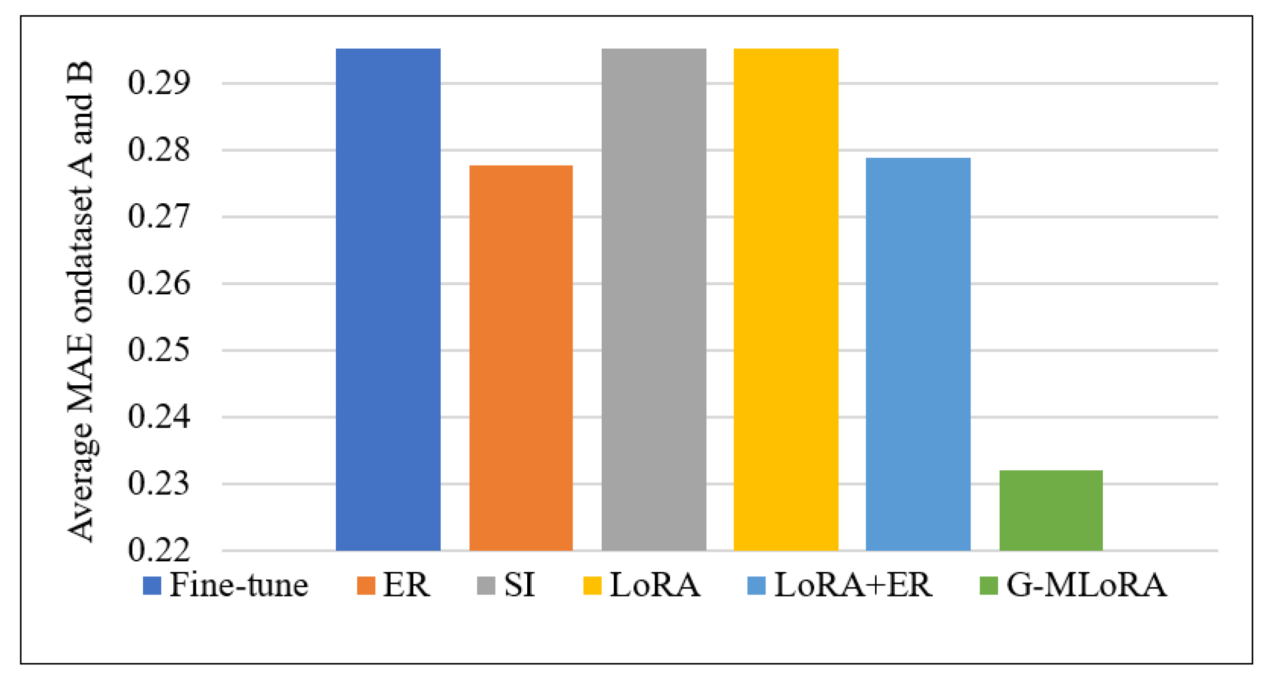
Baseline adjustment for comparison: because methods such as DER need to use historical hidden features, but in the experiment of this section, the dimension of hidden features will also change due to the dynamic change of input dimensions, making such methods unable to be directly used for continual learning tasks with such dynamic input dimension changes. Therefore, in this section, G-MLoRA is only compared with 5 baseline methods: ordinary fine-tuning, ER, SI, LoRA, and LoRA+ER. The reason is that these methods can be directly used for continual learning in dimension change scenarios more conveniently.

(2)

Baseline method adaptation adjustment: the two methods ER and LoRA+ER will encounter the problem of inconsistent dimensions between historical data and new data, making it difficult to directly use historical data and new data for training together. Therefore, in these baseline methods, the gradient accumulation historical knowledge reuse strategy in Section 2.5.2 is also used to balance new and old knowledge with inconsistent dimensions to ensure fairness.

The experimental results for datasets A and B are shown in Figure 7 and Figure 8, respectively. The comprehensive performance comparison of the error conditions on the two datasets is shown in Figure 9.

Analyzing the experimental results, the following key phenomena can be found:

(1)

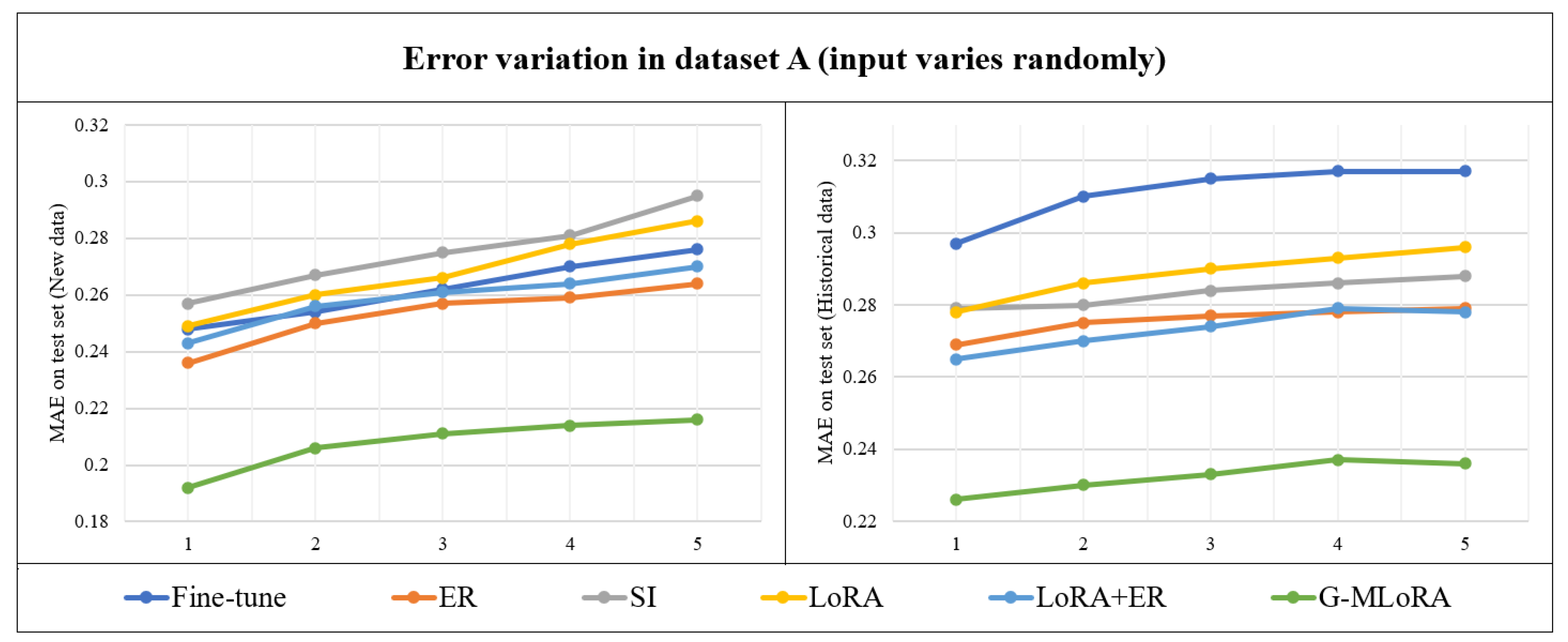
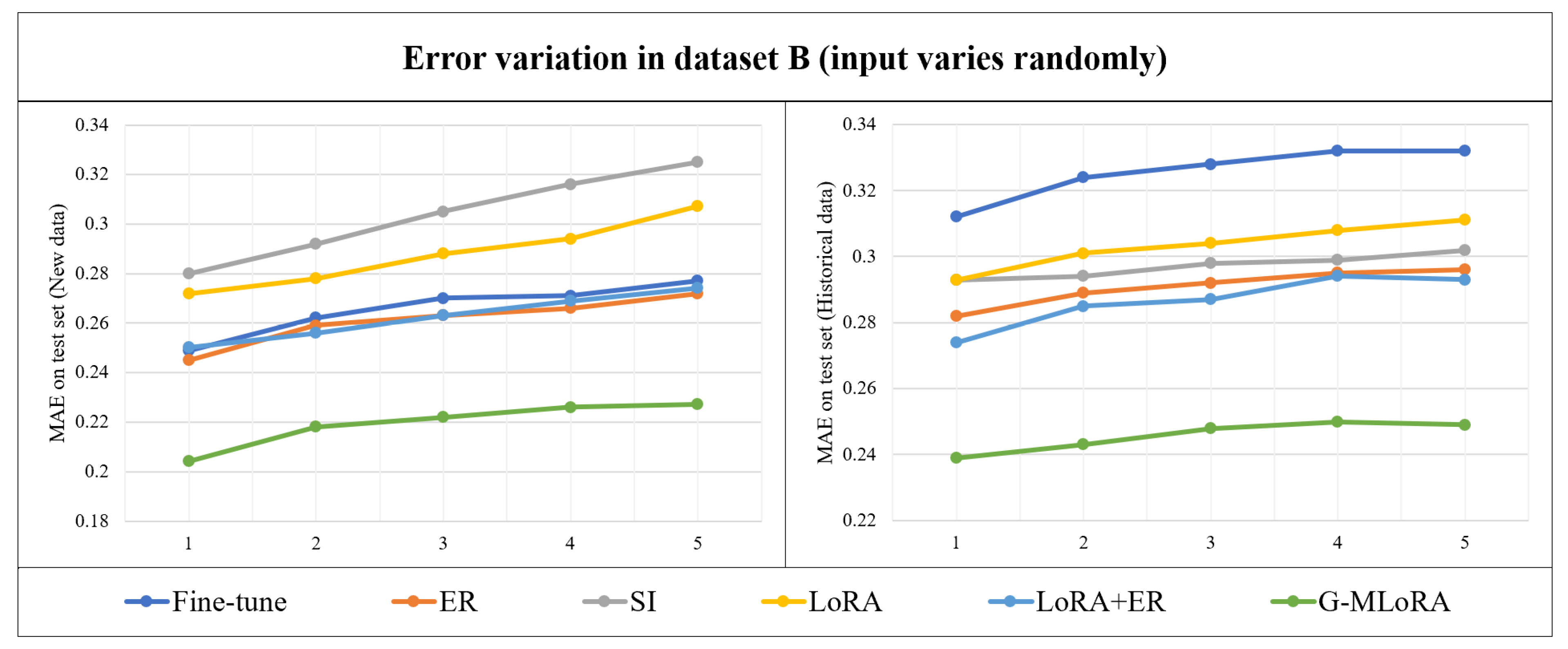
Compared with the experimental results in Section 3.3, the prediction errors of all methods in this section show a more significant upward trend with the increase in task rounds, and the overall errors of all methods are significantly higher than those in the case of fixed input dimensions in Section 3.3. We believe this indicates that dimension changes will significantly increase the difficulty of continual learning and significantly damage the performance of all existing continual learning methods. Dimension changes are an unavoidable phenomenon in practical applications, so this indicates the importance of further researching continual learning methods under dimension change conditions.

(2)

Similar to the phenomenon in Section 3.3, even in the scenario of continuous changes in input dimensions, the three methods ER, LoRA+ER, and G-MLoRA that adopt direct replay of historical samples still achieve relatively better performance. This indicates that even for continual learning tasks in dynamic input dimension scenarios, introducing experience replay is better than relying only on regularization and other means.

(3)

Whether variables are added or missing, the errors of G-MLoRA on the new and old data test sets are significantly lower than other baseline methods. We believe this advantage mainly comes from the introduction of the dynamic grouping strategy to improve the learning effect of variable dependency relationships.

3.5. Comparison of Computational Efficiency of Different Methods

This section compares the average training time per epoch of different methods under fixed input dimensions. The experimental results are shown in Figure 10. It can be seen that the computational efficiency of ordinary LoRA fine-tuning is the highest, even better than ordinary fine-tuning, while the relative time cost of G-MLoRA is higher. The main reason is that the multi-LoRA strategy needs to repeatedly perform LoRA weight loading and unloading operations during each inference. Therefore, this is the focus of further improvement in future research on the proposed method.

After presenting the detailed computation time, we will now analyze in detail the computational complexity of the variable grouping strategy based on Wasserstein distance in this paper in the case of high dimensions.

(1)

Wasserstein distance calculation complexity

For $D$ multivariate time series variables (each of length $L$), pairwise distance computation involves sorting each series ($O\left(L\mathrm{l}\mathrm{o}\mathrm{g}L\right)$) and element-wise difference calculation ($O\left(L\right)$). The total complexity is

$$O\left(D^2\cdot L\mathrm{l}\mathrm{o}\mathrm{g}L\right)$$

(2)

Overall grouping strategy complexity

Integrating distance calculation, K-means clustering ($O\left(Iter\cdot DK\right)$, $Iter$ = K-means iterations), and redundant variable sharing ($O\left(K^{2}D\right)$), the total complexity is

$$O\left(D^2\cdot L\mathrm{l}\mathrm{o}\mathrm{g}L+Iter\cdot DK+K^{2}D\right)$$

(3)

Complexity advantages in high-dimensional scenarios

This grouping strategy reduces the maximum spatial complexity of neural networks for high-dimensional data. By splitting $D$-dimensional variables into $K$ low-dimensional groups (each with $D/K$ variables on average), the data dimension stored during single forward propagation drops from $D$ to $D/K$. Temporally, the overall complexity order remains unchanged, because high-dimensional computation is split into multiple low-dimensional tasks, ensuring efficiency without sacrificing performance.

3.6. Ablation Experiments

To verify the necessity of the two core strategies of G-MLoRA: (1) dynamic clustering grouping and (2) multi-LoRA fine-tuning, this experiment designs 2 groups of ablation variants to compare performance with ordinary G-MLoRA (the average error on all new and old test sets after completing the learning of the 5th batch of new data) to analyze the necessity of the two strategies:

(1)

Variant 1 (G-MLoRA without variable grouping): remove the Wasserstein distance clustering and grouping strategy, adopt full-variable unified inference, and only retain 1 LoRA network, which is equivalent to the LoRA+ER method in the baseline.

(2)

Variant 2 (G-MLoRA without multi-LoRA): only retain 1 LoRA network, and all variable groups are predicted by combining this LoRA network with the backbone, but the inference is performed independently for each group.

Other hyperparameters are consistent with Section 3.3. The experiment is carried out on dataset A, and the experimental results are shown in Figure 11 and

Table 4. Ablation experiment results (MAE on test set after the 5th round of learning on dataset A).

	G-MLoRA	No Grouping	No Multi-LoRA
MAE on new task	0.178	0.27	0.188
MAE on historical task	0.192	0.278	0.202
Average MAE	0.185	0.274	0.195

.

Analyzing the experimental results, the following key phenomena can be found:

(1)

After removing the variable grouping or multi-LoRA strategy, the errors of both new and old data test sets and comprehensive errors increase, indicating the effectiveness of introducing these two strategies in the proposed method.

(2)

The error increase after only removing the variable grouping strategy is significantly higher than that after only removing the multi-group LoRA. We believe the reason is that without grouping, irrelevant variables are forced to fuse data, resulting in redundant information. This is not conducive to forward propagation inference on the one hand, and easily interferes with the compatibility of new and old knowledge during fine-tuning on the other hand, which also indicates the effectiveness of the grouping strategy. Combined with the fact that the multi-LoRA strategy may increase the computational burden shown in Section 3.5, when computational resources are limited and a choice must be made between the two strategies, the variable grouping strategy should be prioritized.

3.7. Hyperparameter Impact Experiments

This experiment explores the impact of the core hyperparameter “number of variable groups (K)” of G-MLoRA on continual learning performance. The values of K are 1, 2, 3, and 4, respectively. Other hyperparameters are consistent with Section 3.3. The evaluation index is “mean of average errors of new and old knowledge” (new knowledge MSE × 0.5 + historical knowledge MSE × 0.5), and the lower the mean, the better the performance. The experimental results are shown in Figure 12.

By observing the experimental results in Figure 12, the following phenomena can be found: (1) When K = 3, the average error of G-MLoRA on the 2 datasets reaches the lowest, while the error is the highest when the number of groups is 8. We believe this is related to the characteristics of the grinding and classification process. From the process perspective, the production processes corresponding to the 2 datasets are composed of three sub-processes: primary grinding, classification, and secondary grinding. Dividing into 3 groups can better group strongly correlated variables into one group. (2) The prediction error increases when the number of groups is 4. We believe this is because excessively fine grouping will force some causally related variables into different groups, making some variables lack key auxiliary information when predicting future states. (3) Overall, the algorithm is quite sensitive to the number of groups of variables. Not grouping or having too many groups will lead to a significant decrease in performance; this demonstrates the effectiveness and importance of introducing grouping strategies in the continuous learning of multivariate time series data in industries such as grinding and classification process. The actual number of groups should be determined according to the characteristics of the corresponding production process. Even when conditions permit, directly using manual redundant grouping may be a more robust and controllable method, and G-MLoRA also supports the direct use of manual grouping for continual learning and prediction in practical applications. However, how to manually divide high-similarity variable groups for the grinding and classification process is not the focus of this paper, so it will not be discussed in detail here.

4. Conclusions

This paper analyzes the limitations of existing methods in dealing with continual learning tasks of dynamic dimensional multivariate time series in process industries and then proposes a continual learning method G-MLoRA based on multi-LoRA fine-tuning and variable grouping strategy, which is applicable to any model with dimensional scalability. By introducing a grouping strategy to reduce redundant variable interference, multi-LoRA learning strategy, and variable-dimensional historical knowledge reuse strategy based on gradient accumulation, G-MLoRA has shown superiority in new and old knowledge compatibility and computational efficiency on 2 real grinding and classification process datasets.

However, the experimental section also indicates three limitations of G-MLoRA: (1) Due to the introduction of the multi-LoRA switching mechanism and additional variable grouping strategy, the computational efficiency of G-MLoRA is lower than that of most current mainstream methods. (2) G-MLoRA is relatively sensitive to the selection of K, a key hyperparameter representing the number of groups. In practical applications, the value of K needs to be properly selected according to the specific applied process to ensure the algorithm achieves optimal performance. (3) Currently, G-MLoRA lacks a targeted identification strategy for noisy variables, but since the dynamic clustering method in this paper can flexibly adapt to changes in input dimensions, similarly, before new variables need to be clustered, some noise identification or filtering algorithms can be directly integrated. After identification or filtering, clustering grouping and subsequent learning are performed. That is to say, G-MLoRA is fully dynamically pluggable for such anti-noise algorithms. In addition, G-MLoRA still faces a balance problem between buffer pool size and long-term historical knowledge storage pressure when dealing with ultra-long-term continual learning tasks. Therefore, in the next stage, we plan to combine few-shot meta-learning technology with grouped continual learning to alleviate the pressure of historical knowledge storage through few-shot learning technology on the basis of balancing the learning of dynamic inter-variable relationships and obtain better long-term historical knowledge retention ability. Additionally, we will also investigate how to effectively identify interfering variables or invalid variables during the variable incremental learning process, so as to avoid mixing in noise information that affects the effect of continual learning.

References

- Wang, Y.; Wang, X.; Zhou, J.; Yang, C.; Yang, Y. Long sequence multivariate time-series forecasting for industrial processes using sasgnn. IEEE Trans. Ind. Inform. 2024, 20, 12407–12417. [Google Scholar] [CrossRef] [Scilit]
- Zhang, Z.; Geng, Z.; Han, Y. Graph structure change-based anomaly detection in multivariate time series of industrial processes. IEEE Trans. Ind. Inform. 2024, 20, 6457–6466. [Google Scholar] [CrossRef] [Scilit]
- Wang, Q.; Sun, J.; Hu, Y.; Jiang, W.; Zhang, X.; Wang, Z. Deep learning-based flatness prediction via multivariate industrial data for steel strip during tandem cold rolling. Expert Syst. Appl. 2024, 237, 121777. [Google Scholar] [CrossRef] [Scilit]
- Zhou, J.; Wang, X.; Yang, C.; Xiong, W. A novel soft sensor modeling approach based on difference-LSTM for complex industrial process. IEEE Trans. Ind. Inform. 2021, 18, 2955–2964. [Google Scholar] [CrossRef] [Scilit]
- Riemer, M.; Cases, I.; Ajemian, R.; Liu, M.; Rish, I.; Tu, Y.; Tesauro, G. Learning to Learn without Forgetting by Maximizing Transfer and Minimizing Interference. In Proceedings of the International Conference on Learning Representations, New Orleans, LA, USA, 6–9 May 2019. [Google Scholar]
- Hinton, G.; Vinyals, O.; Dean, J. Distilling the knowledge in a neural network. arXiv 2015, arXiv:1503.02531. [Google Scholar]
- Buzzega, P.; Boschini, M.; Porrello, A.; Abati, D.; Calderara, S. Dark experience for general continual learning: A strong, simple baseline. Adv. Neural Inf. Process. Syst. 2020, 33, 15920–15930. [Google Scholar]
- Rebuffi, S.-A.; Kolesnikov, A.; Sperl, G.; Lampert, C.H. iCaRL: Incremental classifier and representation learning. In Proceedings of the IEEE Conference on Computer Vision and Pattern Recognition, Honolulu, HI, USA, 21–26 July 2017. [Google Scholar]
- Zhuo, T.; Cheng, Z.; Gao, Z.; Fan, H.; Kankanhalli, M. Continual learning with strong experience replay. arXiv 2023, arXiv:2305.13622. [Google Scholar]
- Arani, E.; Sarfraz, F.; Zonooz, B. Learning Fast, Learning Slow: A General Continual Learning Method based on Complementary Learning System. In Proceedings of the International Conference on Learning Representations, Virtual, 25–29 April 2022. [Google Scholar]
- Wu, M.; Zhou, X.; Li, S.; Shi, H. An adaptive continual learning method for nonstationary industrial time series prediction. IEEE Trans. Ind. Inform. 2024, 21, 1160–1169. [Google Scholar] [CrossRef] [Scilit]
- Aljundi, R.; Belilovsky, E.; Tuytelaars, T.; Charlin, L.; Caccia, M.; Lin, M.; Page-Caccia, L. Online continual learning with maximal interfered retrieval. In Advances in Neural Information Processing Systems; Curran Associates, Inc.: Red Hook, NY, USA, 2019; Volume 32, Available online: https://dlnext.acm.org/doi/10.5555/3454287.3455350 (accessed on 11 February 2026).
- You, X.; Zhang, M.; Ding, D.; Feng, F.; Huang, Y. Learning to learn the future: Modeling concept drifts in time series prediction. In Proceedings of the 30th ACM International Conference on Information & Knowledge Management, Virtual, 1–5 November 2021. [Google Scholar]
- Zenke, F.; Poole, B.; Ganguli, S. Continual learning through synaptic intelligence. In Proceedings of the International Conference on Machine Learning, Sydney, Australia, 6–11 August 2017; PMLR: Cambridge, MA, USA, 2017. [Google Scholar]
- Aljundi, R.; Babiloni, F.; Elhoseiny, M.; Rohrbach, M.; Tuytelaars, T. Memory aware synapses: Learning what (not) to forget. In Proceedings of the European Conference on Computer Vision (ECCV), Munich, Germany, 8–14 September 2018. [Google Scholar]
- Pham, Q.; Liu, C.; Sahoo, D.; Hoi, S.C. Learning fast and slow for online time series forecasting. arXiv 2022, arXiv:2202.11672. [Google Scholar]
- Lea, C.; Vidal, R.; Reiter, A.; Hager, G.D. Temporal convolutional networks: A unified approach to action segmentation. In Proceedings of the European Conference on Computer Vision, Amsterdam, Netherlands, 8–16 October 2016; Springer International Publishing: Cham, Switzerland, 2016. [Google Scholar]
- Gupta, D.; Bhatti, A.; Parmar, S. Beyond LoRA: Exploring Efficient Fine-Tuning Techniques for Time Series Foundational Models. arXiv 2024, arXiv:2409.11302. [Google Scholar]
- Gupta, D.; Bhatti, A.; Parmar, S.; Dan, C.; Liu, Y.; Shen, B.; Lee, S. Low-rank adaptation of time series foundational models for out-of-domain modality forecasting. In Proceedings of the 26th International Conference on Multimodal Interaction, San José, Costa Rica, 4–8 November 2024. [Google Scholar]
- Zhang, J.; Gao, J.; Ouyang, W.; Zhu, W.; Leong, H.Y. Time-llama: Adapting large language models for time series modeling via dynamic low-rank adaptation. In Proceedings of the 63rd Annual Meeting of the Association for Computational Linguistics (Volume 4: Student Research Workshop), Vienna, Austria, 27 July–1 August 2025. [Google Scholar]
- Hu, E.J.; Shen, Y.; Wallis, P.; Allen-Zhu, Z.; Li, Y.; Wang, S.; Wang, L.; Chen, W. Lora: Low-rank adaptation of large language models. ICLR 2022, 1, 3. [Google Scholar]
- Wickramasinghe, B.; Saha, G.; Roy, K. Continual learning: A review of techniques, challenges, and future directions. IEEE Trans. Artif. Intell. 2023, 5, 2526–2546. [Google Scholar] [CrossRef] [Scilit]
- Ao, S.-I.; Fayek, H. Continual deep learning for time series modeling. Sensors 2023, 23, 7167. [Google Scholar] [CrossRef] [Scilit] [PubMed]
- Lou, X.; Zan, H.; Wang, Z.; Shi, J.; Zhang, S. Privacy-Preserving Bidirectional Data Transmission of Smart Grid via Semi-Quantum Computation: On Mutual Identity and Message Authentication. IEEE Trans. Dependable Secur. Comput. 2025, 22, 5537–5548. [Google Scholar] [CrossRef] [Scilit]
- Nie, Y. A Time Series is Worth 64Words: Long-term Forecasting with Transformers. arXiv 2022, arXiv:2211.14730. [Google Scholar]
- Zhou, X.; Wang, W.; Buntine, W.; Qu, S.; Sriramulu, A.; Tan, W.; Bergmeir, C. Scalable transformer for high dimensional multivariate time series forecasting. In Proceedings of the 33rd ACM International Conference on Information and Knowledge Management, Boise, ID, USA, 21–25 October 2024. [Google Scholar]
- Liu, Y.; Hu, T.; Zhang, H.; Wu, H.; Wang, S.; Ma, L.; Long, M. itransformer: Inverted transformers are effective for time series forecasting. arXiv 2023, arXiv:2310.06625. [Google Scholar]
- Dong, J.; Liu, Y.; Long, M.; Qin, G.; Qiu, Y.; Wang, J.; Wang, Y.; Wu, H.; Zhang, H. Timexer: Empowering transformers for time series forecasting with exogenous variables. Adv. Neural Inf. Process. Syst. 2024, 37, 469–498. [Google Scholar]
- Han, L.; Ye, H.-J.; Zhan, D.-C. The capacity and robustness trade-off: Revisiting the channel independent strategy for multivariate time series forecasting. IEEE Trans. Knowl. Data Eng. 2024, 36, 7129–7142. [Google Scholar] [CrossRef] [Scilit]
- Wen, Q.; Chen, W.; Sun, L.; Zhang, Z.; Wang, L.; Jin, R.; Tan, T. Onenet: Enhancing time series forecasting models under concept drift by online ensembling. Adv. Neural Inf. Process. Syst. 2023, 36, 69949–69980. [Google Scholar]
- Gupta, V.; Narwariya, J.; Malhotra, P.; Vig, L.; Shroff, G. Continual learning for multivariate time series tasks with variable input dimensions. In Proceedings of the 2021 IEEE International Conference on Data Mining (ICDM), Virtual, 7–10 December 2021; IEEE: Piscataway, NJ, USA, 2021. [Google Scholar]
- Zhou, J.; Cui, G.; Hu, S.; Zhang, Z.; Yang, C.; Liu, Z.; Wang, L.; Li, C.; Sun, M. Graph neural networks: A review of methods and applications. AI Open 2020, 1, 57–81. [Google Scholar] [CrossRef] [Scilit]
- Li, K.-H. Reservoir-sampling algorithms of time complexity O(n(1+log (n/n))). ACM Trans. Math. Softw. (TOMS) 1994, 20, 481–493. [Google Scholar] [CrossRef] [Scilit]