Robust Multi-Objective Optimization of Ore-Drawing Process Using the OGOOSE Algorithm Under an ε-Constraint Framework

Abstract

To address the complex multi-objective optimization problem of “cost–risk–recovery–dilution” in sublevel caving without bottom pillars under uncertainty, this study develops an operational GOOSE-based framework (OGOOSE) integrated with robust ε-constraint modeling. Methodologically, OGOOSE adopts three synergistic mechanisms: Opposition-Based Learning (OBL) for enhanced initial solution quality and spatial coverage symmetry, an Adaptive Inertia Weight (AIW) mechanism to maintain a symmetrical balance between exploration and exploitation, and a Boundary Reflection Mechanism (BRM) to ensure engineering feasibility. For modeling, an “ellipsoid-plane” geometric surrogate is employed, where the ellipsoid’s structural symmetry serves as the ideal baseline, while the Mean-CVaR criterion quantifies the asymmetry of operational risk (negative tail) under uncertainty. Taking robust cost (C) as the primary objective, the four-objective problem is decomposed via the ϵ-constraint method to enforce a balanced Pareto trade-off. Results demonstrate that OGOOSE significantly outperforms GOOSE, WOA, and HHO on CEC2017 benchmarks, achieving the lowest Friedman rank. In the engineering case study, it attains an average dilution rate of 28.95% (the lowest among comparators) without increasing unit cost or compromising recovery, demonstrating stable operational symmetry across economic and quality indicators. Sensitivity analysis of the ε-thresholds identifies an optimal “knee-point” that establishes a manageable balance between risk control (εR) and dilution limits (εP). OGOOSE effectively balances accuracy, stability, and interpretability, providing a robust tool for stabilizing complex mining systems against inherent operational asymmetry.

1. Introduction

The Sublevel Caving (SLC) method without bottom pillars is widely adopted in the mining industry for its operational safety, high production intensity, and cost efficiency, making it particularly suitable for extracting steeply inclined, thick orebodies. Unlike open stoping methods, SLC relies on drawing ore under a blanket of caved waste rock, which makes ore loss and dilution inevitable consequences of the gravity flow process. The efficiency of this system depends critically on structural parameters, specifically the caving step distance and drift spacing. While drift spacing is typically constrained by geological conditions and equipment dimensions, the caving step distance remains a flexible and decisive lever for regulating the extraction process. Consequently, determining an optimal caving step is a complex decision problem of significant practical importance, requiring a careful balance between resource recovery and product quality. However, traditional deterministic optimization approaches are increasingly insufficient for SLC design, as they fail to account for the complex and dynamic uncertainties inherent in the underground mining environment.

Crucially, pervasive geological and operational fluctuations induce a phenomenon defined in this study as systemic operational asymmetry. Unlike symmetric Gaussian noise, this asymmetry is mathematically characterized by significant negative skewness and heavy-tailed distributions in the performance indicators. In the context of sublevel caving, the loss function is inherently asymmetric: A minor deviation in the caving step can lead to a disproportionate spike in dilution or a collapse in recovery (the “negative tail”), whereas a precise optimization yields only marginal economic gains. Recent studies have demonstrated that ignoring this asymmetry deteriorates optimization performance. To address these challenges, various robust frameworks have been proposed. While recent works such as Bafghi et al. (2025) [1] have successfully applied Fuzzy Robust Optimization to manage parameter vagueness in open-pit scenarios, this study focuses on the stochastic nature of sublevel caving, where the risk profile is driven by probabilistic distributional tails rather than membership ambiguity.

Consequently, traditional optimization methods based on mean values or standard deviations are insufficient, as they treat positive and negative deviations equally. To restore the necessary structural equilibrium, this study adopts a robust Mean-CVaR (Mean-Conditional Value at Risk) formulation. Aligning with the cutting-edge simulation optimization methodologies proposed by Hu et al. (2025) [2], CVaR is explicitly selected over variance because it is a coherent risk measure capable of quantifying the tail risk—specifically, the expected loss exceeding a certain confidence level (β). This mathematical property allows the optimizer to focus specifically on truncating the “negative tail” caused by systemic asymmetry, thereby stabilizing parameters against extreme worst-case scenarios rather than average fluctuations.

Integrating this Mean-CVaR robustness into a multi-objective framework transforms parameter optimization into a highly nonlinear, multimodal, and computationally expensive landscape. Since the 1990s, swarm intelligence algorithms have attracted widespread attention for such complex engineering problems due to their gradient-free search capabilities, with successful applications ranging from path planning [3] and energy storage configuration [4] to intelligent scheduling [5] and global optimization [6]. Among these, the Goose Optimization Algorithm (GOOSE), recently proposed by [7], has shown particular promise due to its balanced mechanism of group guidance and exploration. However, standard swarm algorithms, including GOOSE, often struggle with the specific demands of robust mining optimization: they are prone to premature convergence in high-noise environments and lack specific mechanisms to strictly enforce engineering feasibility constraints. To effectively navigate the conflicting trade-offs of “cost–risk–recovery–dilution”, the base algorithm requires structural enhancements to improve its initialization quality, search rhythm, and boundary handling capabilities.

To address these challenges, this study proposes a comprehensive multi-objective robust optimization framework structured across three levels: “algorithm, modeling, and solution.” At the algorithm level, an Operational GOOSE (OGOOSE) variant is developed. It incorporates three synergistic design levers: Opposition-Based Learning (OBL) to ensure high-quality initialization and spatial symmetry in coverage; an Adaptive Inertia Weight (AIW) mechanism to unify control over the search rhythm; and a Boundary Reflection Mechanism (BRM) to guarantee feasibility. At the modeling level, an “ellipsoid-plane” geometric surrogate is adopted to ensure continuous differentiability and dimensional consistency in calculating recovery and dilution rates. Finally, at the solution level, the ε-constraint method is employed to decompose the four-objective problem. By treating robust cost as the primary objective and converting risk, dilution, and recovery into threshold constraints, this approach unifies evaluation standards and provides an interpretable tool for engineering parameter adjustment (εR, εP).

2. Methodology

2.1. GOOSE Optimization Algorithm

The GOOSE optimization algorithm is inspired by the natural behavior of goose flocks, particularly their protective mechanisms during rest and foraging. It consists of two phases: the exploitation phase (global search) and the exploration phase (local search).

(1)

Development stage: A random weight $W_1$ of stones randomly obtained by sentinel geese is selected, ranging from 5 to 25, with the specific calculation formula as Equation (1):

$$W_1=\mathrm{randi}\left(\right[5, 25], 1 , 1)$$

(1)

Calculate the time $T_1$ required for the stone to fall, as shown in Equation (2):

$$T_1 = \mathrm{rand}(1 , \mathit{dim})$$

(2)

where $\mathit{dim}$ is the dimension of the objective function.

Then calculate the time $T_2$ for the sound to propagate to a random goose after the stone falls, as shown in Equation (3):

$$T_{2 }= \mathrm{rand}(1 , \mathit{dim})$$

(3)

Next, calculate the total time $T_t$ for the sound to propagate to each individual in the flock throughout the iteration process, as shown in Equation (4), and then the required average time $T_3$ can be obtained as shown in Equation (5):

$$T_t = {\displaystyle \frac{\sum (T_2)}{\mathit{dim}}}$$

(4)

$$T_3={\displaystyle \frac{T_t}{2}}$$

(5)

Then, calculate the falling speed $V_1$ of the stone randomly obtained by the sentinel goose. A random variable pro (uniformly distributed in [0, 1]) is introduced here. When pro > 0.2 and $W_1$ ≥ 12, the corresponding calculation formula is as follows:

$$V_1 = T_1 · {\displaystyle \frac{\sqrt{W_1}}{9.81}}$$

(6)

where the constant 9.81 is treated strictly as a dimensionless heuristic scalar to normalize the object weight, ensuring mathematical coherence without dimensional inconsistency.

Subsequently, calculate the distance $D_1$ that the sound travels from the stone falling from the sentinel goose’s foot to a certain goose, as shown in Equation (7):

$$D_1 = S_1 · T_1$$

(7)

where $S_1$ represents the sound propagation coefficient, set to the scalar value of 343.2. While inspired by sound speed, this parameter functions here as a long-range exploration multiplier. Any resulting step sizes exceeding the search space are subsequently corrected by the Boundary Reflection Mechanism (BRM) (Section 2.5) to guarantee feasibility.

After obtaining the sound propagation distance from Equation (7), the distance between the sentinel goose and another goose can be calculated as follows:

$$D_2 = {\displaystyle \frac{1}{2}} · D_1$$

(8)

A random variable, rnd, is introduced to balance the exploration and exploitation phases. When $\mathit{rnd} \ge 0.5$, the algorithm enters the exploitation phase. At this time, if $\mathit{pro} > 0.2$ and $W_1 \ge 12$, a new optimal $X_{t + 1}$ can be calculated using Equation (9), which consists of the falling speed $V_1$ of the object plus the product of the distance $D_1$ of the goose and the square of the average time $T_3$:

$$X_{t + 1} = V_1 + D_{1 }{· T}_3^2$$

(9)

When $\mathit{pro} < 0.2$ and $W_{1 }< 12$, update the speed $V_2$ of the stone reaching the ground under this condition, as shown in Equation (10):

$$V_2 ={ T}_1 · {\displaystyle \frac{W_1}{9.81}}$$

(10)

Under the condition of Equation (11), a variable $\mathit{coe}$ (a random number between 0 and 1) is introduced, and the calculation process for the updated $X_{\mathrm{best}}$ is shown in Equation (11):

$$X_{t + 1} = V_2 · D_1 · T_3^2 · \mathit{coe}$$

(11)

(2)

Exploration stage: When the random variable $\mathit{rnd} < 0.5$, the algorithm enters this phase. The goose flock adjusts the position of a randomly awakened goose or sentinel goose according to the currently found optimal position. A variable $\alpha$ is introduced to improve the new $X$ result in the search space, with values ranging from 2 to 0. As iterations proceed, the value of $\alpha$ decreases sharply until it approaches 0.

$$\alpha =\left(2-{\displaystyle \frac{2\hspace{0.17em}t}{T_{\max }}}\right)$$

(12)

where $t$ is the current number of iterations, and $T_{\max }$ is the maximum number of iterations.

The updated position of $X$ in this phase is $X_{t + 1}$, calculated as shown in Equation (13):

$$X_{t + 1} = \mathrm{randn}(1 , \mathit{dim}) · \left(T_{\min } · \alpha \right) + X_{\mathrm{best}}$$

(13)

where $T_{\min }$ is the minimum time required to awaken the goose flock, and X_best is the optimal position of $X$ found in the search space.

2.2. Optimization Framework of the OGOOSE Algorithm

Based on the original GOOSE algorithm, an optimization framework composed of three modules (OBL population initialization, adaptive exploration-exploitation weighting mechanism, and boundary reflection mechanism) is introduced, which retains structural simplicity while enhancing the ability to find optimal solutions in complex spaces. These three modules are widely applicable in most algorithms, and this study combines them for application: the Opposition-Based Learning (OBL) mechanism screens the generated population before entering the main loop, improving the quality and coverage of initial solutions in the search space and achieving better spatial symmetry; the adaptive exploration-exploitation weighting mechanism runs through the entire main loop process to maintain a dynamic symmetrical balance in the step size and timing of the exploration and exploitation phases, avoiding excessive bias towards either phase; the boundary reflection mechanism acts after each position update but before objective function evaluation, ensuring the optimal solution search remains within the feasible region, avoiding invalid evaluation of out-of-bounds solutions, smoothing the convergence curve, and improving feasibility and evaluation efficiency.

2.3. OBL Population Initialization

In the later stages of algorithm iteration, randomly initialized populations often exhibit uneven distribution, making the algorithm prone to premature convergence and low solution precision. To address this issue, the Opposition-Based Learning (OBL) mechanism [8] is adopted to initialize the population. For each randomly generated individual, its opposite point with respect to the center of the search space is also computed, and the better one is retained. This process ensures that OBL generates an initial population possessing topological symmetry relative to the center of the search domain, which dramatically improves the spatial coverage and balance of initial solutions, effectively minimizing initial bias toward local optima. This procedure improves the spatial coverage of the initial population and enhances its diversity and stability.

In this study, OBL is applied to the initial population rather than to the personal best position ($X_{\mathrm{best}}$) of individuals, which eliminates the need to maintain historical bests and keeps the algorithmic structure simple while enhancing its performance on shifted, rotated, and composite benchmark functions.

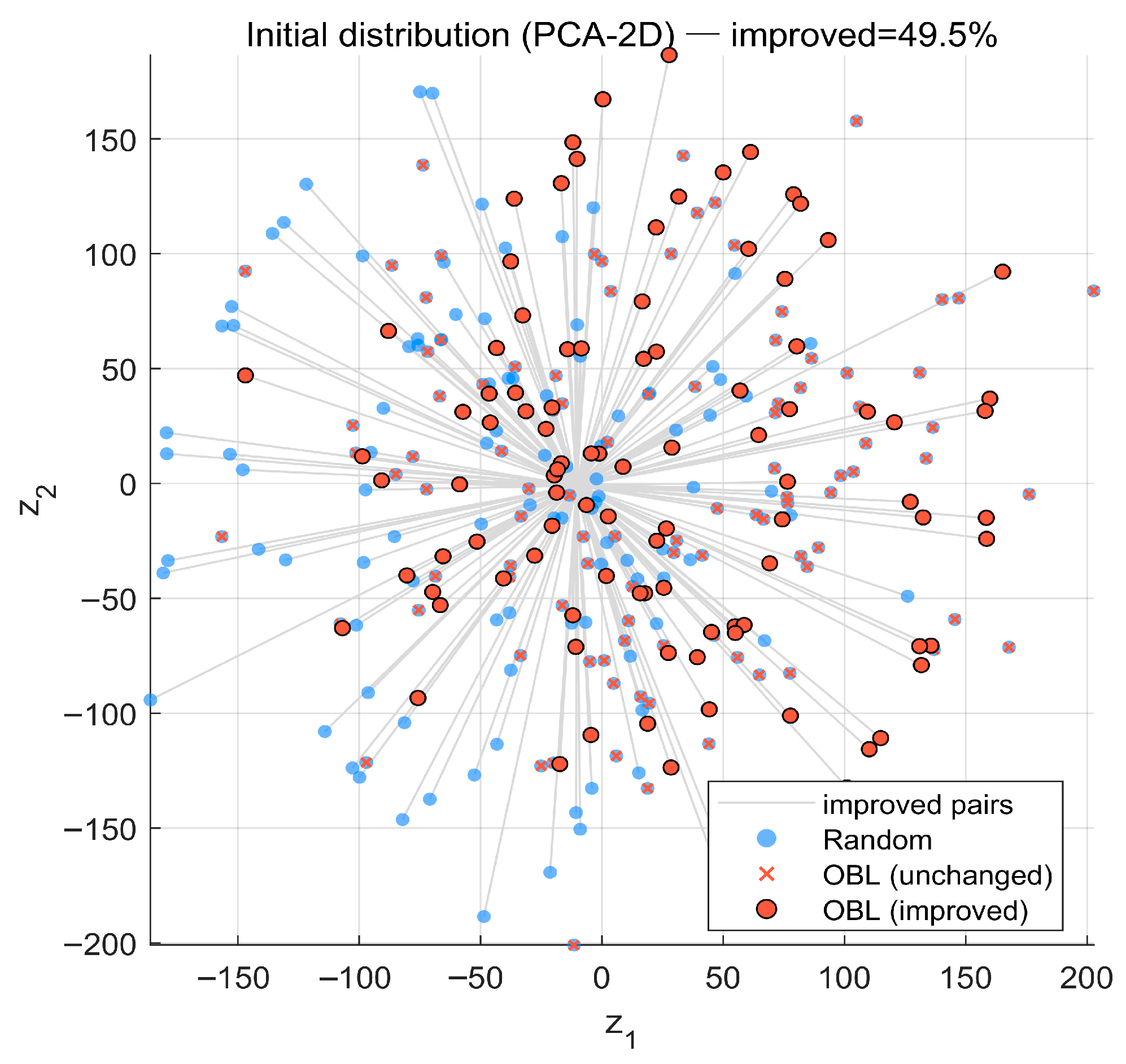
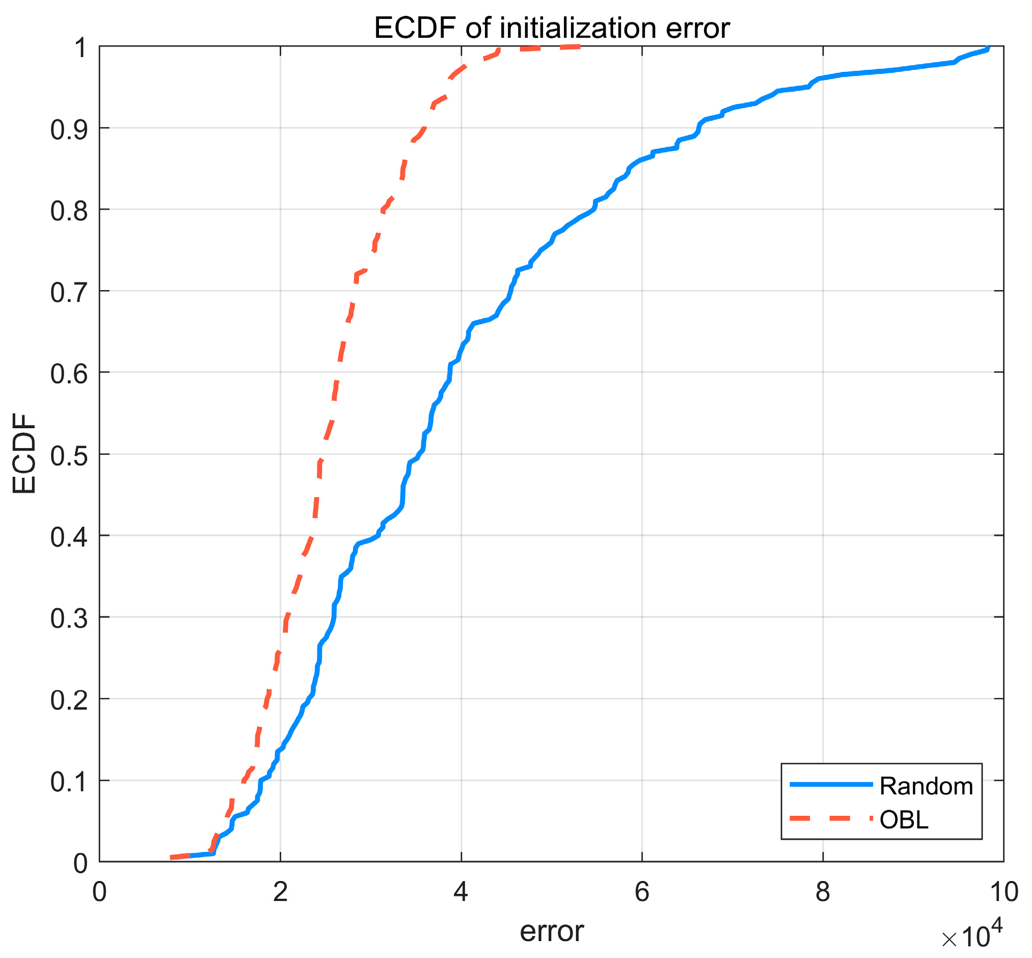
The original GOOSE algorithm employs purely random initialization, which may result in non-uniform population distribution and convergence to local optima. To examine the difference between random and OBL-based initialization, Composition Function 6 from the CEC2017 test suite (dim = 50, population size N = 200) is used to evaluate the quality of initial solutions, as shown in Figure 1 and Figure 2.

Figure 1 illustrates the spatial distribution of initial populations, where approximately 49.5% of random individuals are improved through OBL. The variance of randomly initialized solutions is 1.940 × 10⁴, while that of OBL-initialized solutions is 7.577 × 10³—a reduction of about 61%. A Wilcoxon signed-rank test on paired objective values yields p = 3.16 × 10⁻³⁰ (≪0.01), confirming that OBL initialization significantly outperforms random initialization. Figure 2 presents the ECDF (Empirical Cumulative Distribution Function) of initialization errors, showing that the OBL curve consistently lies above and to the left of the random curve across the entire range, demonstrating that OBL achieves superior population distribution and initialization quality.

2.4. Adaptive EXPLORATION-Exploitation Weighting Mechanism

To improve the balance between exploration and exploitation during the optimization process, an adaptive exploration-exploitation weighting mechanism is introduced into the GOOSE algorithm. Unlike a simple linear decay, this adaptive weight dynamically updates after each iteration. Specifically, the primary objective of this mechanism is to maintain a dynamic symmetrical balance of search rhythm throughout the process. A larger weight is used in the early stage to encourage global exploration (breaking local constraints), a moderate weight in the middle stage to sustain this symmetry and avoid premature convergence, and a smaller weight in the later stage to enhance local exploitation (consolidating the equilibrium point).

The adaptive weight strategy adopted in this study combines two components: linear annealing—a temperature-inspired decay mechanism originating from simulated annealing [9]—and logistic chaotic mapping, a nonlinear dynamic system capable of generating aperiodic and ergodic sequences [10]. The key innovation lies in consistently incorporating this adaptive weight into all three position update schemes of the GOOSE algorithm, enabling unified regulation of exploration and exploitation intensity.

At the beginning of each iteration, the adaptive exploration-exploitation weighting mechanism $w_{\mathrm{t}}$ is computed and applied uniformly to all individuals. Its formulation is as follows:

$$Z_{t + 1 }= 4 · Z_t (1- Z_t), Z_t\in (0, 1)$$

(14)

$$w_{\mathrm{lin}}(t)=w_{\max }-\left(w_{\max }-{ w}_{\min }\right) {\displaystyle \frac{t- 1}{T_{\max }- 1}}$$

(15)

$$w_t ={\alpha }_{\mathrm{mix}} · w_{\mathrm{lin}}(t)+\left(1 -{\alpha }_{\mathrm{mix}}\right)\left(0.5+0.5Z_{t+1}\right)$$

(16)

where $Z_t$ is the logistic chaotic variable at iteration $t$, $Z_{t + 1}$ is its mapped value in the next generation, $w_{\mathrm{lin}}\left(t\right)$ denotes the linear annealing baseline weight, $w_{\max }=0.9$ and $w_{\min }=0.4$ are the upper and lower bounds of the weight, and ${\alpha }_{\mathrm{mix}}=0.5$ is the mixing coefficient.

Equation (14) defines the logistic chaotic sequence that introduces aperiodic perturbations within the range (0, 1). Equation (15) establishes the baseline weight that linearly decreases over iterations, following the principle of simulated annealing [9]. Equation (16) integrates both components through a weighted combination, yielding an adaptive weight shared by all individuals in each iteration, thereby enhancing search adaptability and convergence precision.

When the conditions $W_1 \ge 12$, $\mathit{rnd} \ge 0.5$ and $pro > 0.2$ are satisfied simultaneously, the algorithm enters the strong-attraction update phase, in which the new position of the i-th agent is computed according to Equation (17). At this stage, the GOOSE algorithm is in the exploitation phase, where each individual $x_{\mathrm{i}}^{\mathrm{t}}$ moves toward the target position $X_{t+1}$ through a convex combination movement. The direction of movement is determined by $X_{t+1}-X_i^t$, and the step length is scaled by the adaptive weight $w_t\left(X_{t+1}-x_{\mathrm{i}}^{\mathrm{t}}\right)$. The update rule is given by

$$X_i^{ t+1}=X_i^{ t}+{ w}_t\left(X_{t+1}-X_{ i}^{ t}\right)$$

(17)

where $X_i^t$ and $X_i^{t + 1}$ denote the actual positions of the i-th individual in the t-th and (t + 1)-th generations, respectively; $X_i^{t + 1}$ is obtained from Equation (9).

When $\mathit{rnd} \ge 0.5$ and either $W_1<12$, $pro<0.2$, the algorithm performs a weak-step update, whose position change is defined by Equation (18). The GOOSE algorithm remains in the exploitation phase, executing small-step fine-tuning around the current position to achieve stable local refinement. The movement amplitude is governed by the adaptive weight ${ w}_t$, while the step magnitude is constrained by coefficient coe. The update equation is formulated as

$${\mathit{X}}_i^{t+1}={\mathit{X}}_i^t+{\mathrm{w}}_{\mathrm{t}}{\mathit{X}}_{t+1}$$

(18)

where ${\mathit{X}}_i^{t + 1}$ is determined according to Equation (11).

When $\mathit{rnd} < 0.5$, the algorithm transitions into the Gaussian exploration update phase, corresponding to the exploration stage of the search process. In this case, Gaussian diffusion is conducted around the global best position of the current iteration.

When the condition $\mathit{rnd} < 0.5$ is met, the GOOSE algorithm initiates the exploration phase by triggering a Gaussian exploration position update. This involves performing Gaussian diffusion centered on the global optimum of the current iteration to achieve a diversified search. The diffusion radius is primarily controlled by $T_{\min }$ and ${\alpha }_t$, while the entire exploration scale is further regulated by W₁, ensuring that the search space gradually contracts as the number of generations increases (annealing). The sampling rule of this Gaussian exploration is mathematically summarized in Equations (19) and (20).

$${\mathsf{\eta }}_{\mathrm{i}}^t ~ \mathrm{N}\left(0 , (T_{\min }{\alpha }_t{)}^2 · {\mathrm{I}}_D\right)$$

(19)

$${\mathit{X}}_i^{t+1}={\mathit{X}}_{\mathrm{best}} +{\mathrm{w}}_{\mathrm{t}}{\mathsf{\eta }}_{\mathrm{i}}^{\mathrm{t}}$$

(20)

where $T_{\min }$ represents the lower bound of the time scale in the current generation, calculated as the minimum value from Equation (4);${\alpha }_t$ denotes the exploration-scale annealing factor obtained from Equation (12); ${\mathsf{\eta }}_{\mathrm{i}}^t$ is the Gaussian exploration step derived from the standard normal vector $\mathit{z}$ through linear scaling according to Equation (13); and ${\mathrm{I}}_D$ is the identity matrix.

2.5. Boundary Reflection

In the GOOSE algorithm, candidate solutions may occasionally exceed the predefined search domain during position updates. To ensure feasibility, a boundary reflection mechanism [11] is applied, guaranteeing the structural integrity of the search process and ensuring that the operational model remains within the defined bounds. This prevents solutions from violating the feasible domain of the problem and avoids unnecessary computational effort on infeasible regions.

When a solution exceeds the lower bound of the search domain, its position is corrected according to

$$x_i = \mathit{lb} + (\mathit{lb} - x)$$

(21)

When a solution exceeds the upper bound, the correction is expressed as

$$x_i= \mathit{ub} - (x - \mathit{ub})$$

(22)

where $x_i$ is the value of the candidate solution after mapping, ub and $\mathit{lb}$ are the upper and lower bounds of the search space, respectively, and $x$ is the value of the candidate solution before mapping.

In cases where a solution greatly deviates from the feasible domain and remains outside the bounds even after reflection, a projection operator is further employed to ensure feasibility through bounded projection:

$$x_{\mathrm{ref}} = \min \left\{\max (x , \mathit{lb}) , \mathit{ub}\right\}$$

(23)

where $x_{\mathrm{ref}}$ denotes the final position after reflection and projection correction.

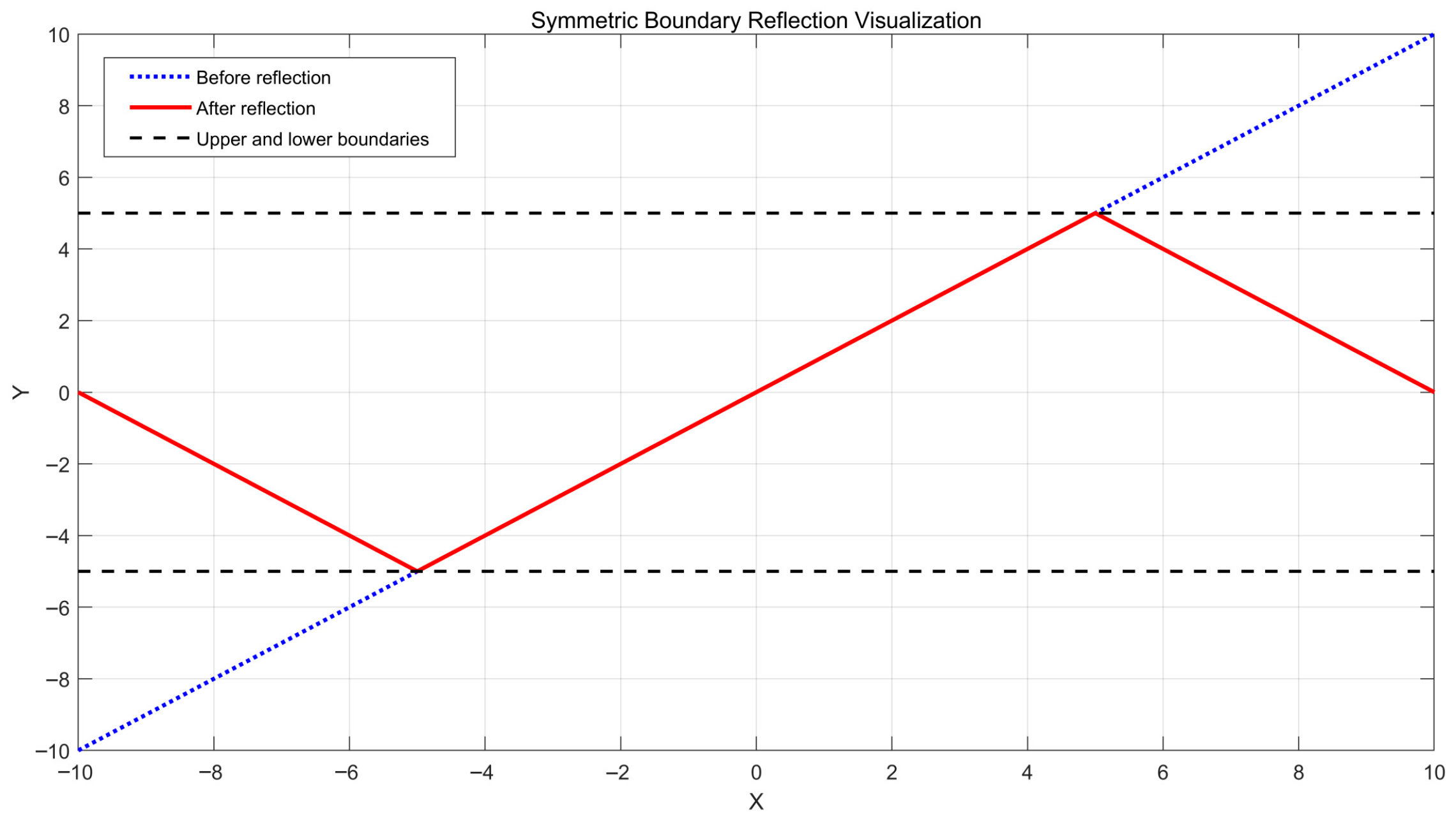
As shown in Figure 3, within the bounded search domain of [−5, 5], all candidate solutions exceeding the domain limits are reflected back into the feasible region through the boundary reflection mechanism. This process effectively steers the search toward the global optimum and prevents the occurrence of numerical instabilities such as overflow, thereby improving the robustness and stability of the algorithm.

2.6. OGOOSE Algorithm Flow

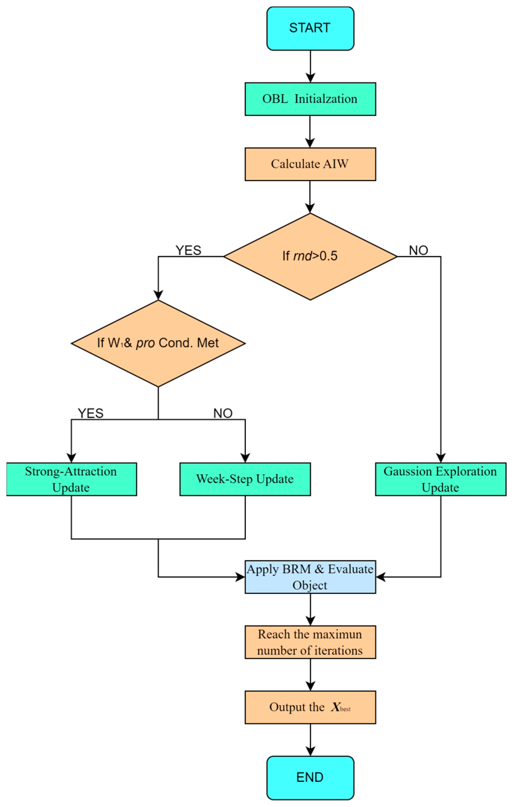
The execution flow of the OGOOSE algorithm is systematically designed to integrate its three synergistic mechanisms, balancing search capability, convergence speed, and solution stability, as summarized in the flowchart shown in Figure 4. To complement this visual overview, the detailed pseudocode of the proposed OGOOSE framework is presented in Appendix A. The process begins with Enhanced Initialization (OBL-based Initialization), where the population is generated using the Opposition-Based Learning (OBL) mechanism to ensure that the individual position vectors $X_i$ possess higher quality and more uniform spatial coverage in the search space. Subsequently, the algorithm enters the Main Iterative Search Loop with Adaptive Weighting (AIW). At the start of each iteration, a scalar Adaptive Exploration–Exploitation weight $w_{\mathrm{t}}$ is computed by combining a linear annealing baseline with a logistic chaotic variable $Z_t$, which is generated through Logistic mapping. This dynamic weight $w_{\mathrm{t}}$ is uniformly embedded into all three position-update strategies of the GOOSE algorithm—strong-attraction, weak-step, and Gaussian-exploration—to regulate the symmetrical balance of the search rhythm for each individual position vector $X_i^{t + 1}$. After every position update $X_i^{t + 1}$ and before the robust objective function evaluation, the Boundary Reflection Mechanism (BRM) is executed to ensure that all solutions remain within the feasible region, thereby improving numerical robustness and maintaining system integrity. This cycle of adaptive weighted updating and boundary correction continues until the maximum number of iterations $T_{\max }$ is reached, after which the best position vector $X_{\mathrm{best}}$ is output as the final global optimum.

2.7. Ablation Experiment on Three Modules

To further evaluate the individual contributions and interaction effects of the three modules on the performance of the GOOSE algorithm, a systematic full factorial (2³) ablation experiment was designed, as shown in

Table 1. Variant Index and Configuration for the 2³ Factorial Ablation Experiments.

Number	Initialization	Weight Strategy	Boundary Strategy
V000	Random Distribution	Constant (w = 1.0)	None
V001	Random Distribution	Constant (w = 1.0)	BRM
V010	Random Distribution	AIW	None
V011	Random Distribution	AIW	BRM
V100	OBL	Constant (w = 1.0)	None
V101	OBL	Constant (w = 1.0)	BRM
V110	OBL	AIW	None
V111	OBL	AIW	BRM

. This orthogonal design framework was selected to rigorously isolate the individual contributions (main effects) of OBL, AIW, and BRM, as well as to detect any potential synergistic or antagonistic interactions among them, thereby eliminating confounding factors. When the OBL-based population initialization module is disabled, a uniformly random distribution is adopted for population initialization. When the adaptive exploration–exploitation weighting mechanism is deactivated, the adaptive weight is fixed at w_t = 1 and remains constant throughout the iterations. When the boundary reflection mechanism is omitted, no boundary-handling strategy is applied.

Table 1 lists the eight unique configurations derived from the 23 Full Factorial Design framework. This specific Design of Experiments (DOE) structure is mathematically chosen to systematically decouple the main effects of each module (OBL, AIW, BRM) from their potential interaction effects. By evaluating the complete set of permutations (from V000 to V111), the experiment ensures a rigorous isolation of algorithmic contributions, verifying whether the performance gain stems from a single dominant mechanism or the synergistic integration of all three components.

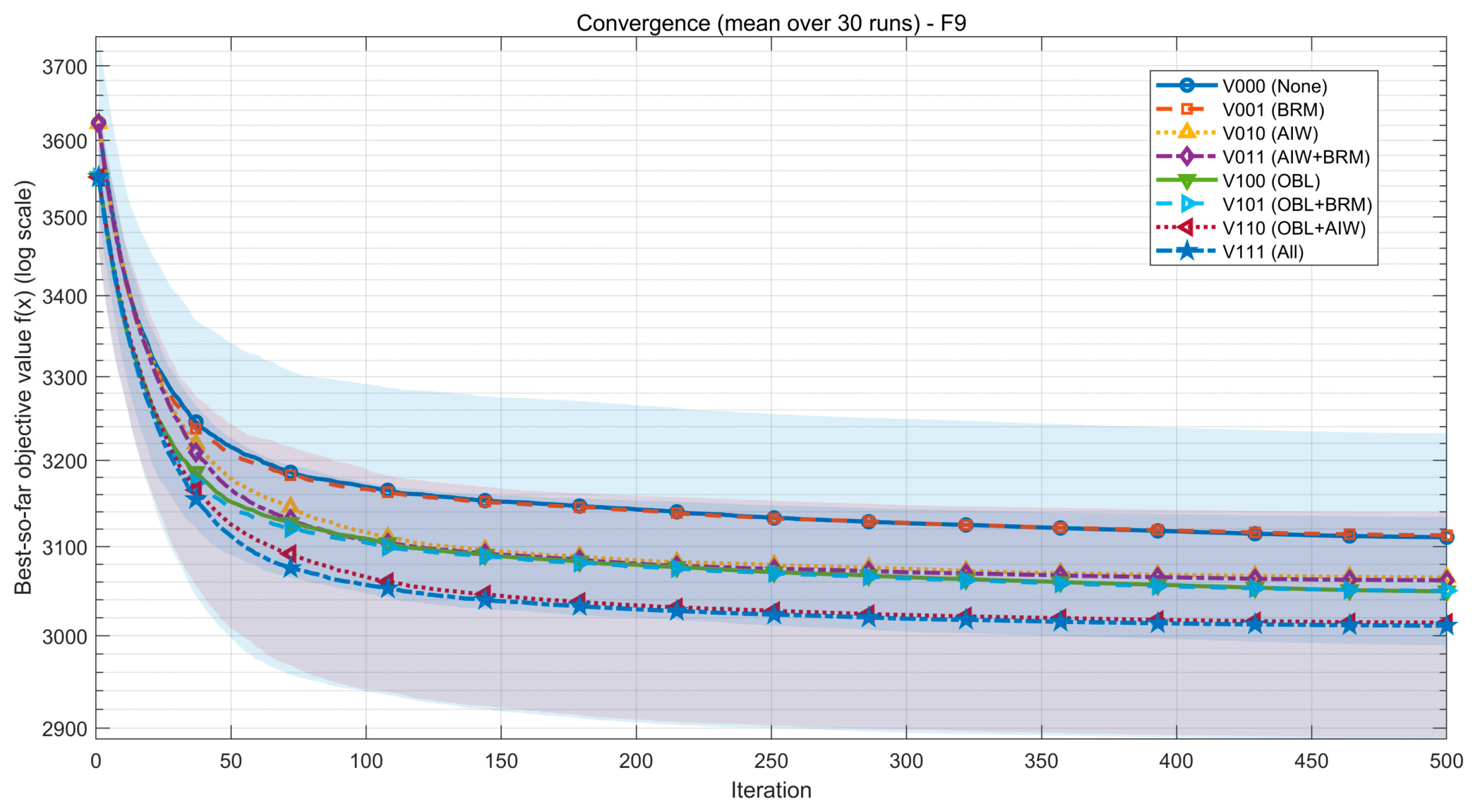
Ablation experiments were performed using the CEC2017 test function F9, i.e., “Composition Function 7” with N = 5 and dim = 50, as the objective function. The experimental parameters were set as follows: problem dimension = 50, population size = 30, maximum iterations = 500, and number of independent runs = 30. Using the original GOOSE algorithm (V000, None) and the full configuration V111 (OBL + AIW + BRM) as reference baselines, the experiment evaluates the performance effects of all single-module and dual-module combinations on the GOOSE algorithm.

As shown in Figure 5, the baseline variant V000 (None) converges noticeably more slowly than the other seven variants over the entire iteration range and attains the highest final best-so-far value. V001 (BRM) shows a slightly faster decrease in the early iterations, but its final objective value is almost identical to that of V000, indicating that BRM alone has little influence on the average optimization outcome in this task.

V010 (AIW) and V100 (OBL) both significantly outperform V000 in terms of convergence and final objective value, and their curves remain consistently below the baseline. This demonstrates that either the adaptive exploration–exploitation weighting mechanism (AIW) or opposition-based initialisation (OBL) can independently improve the search process. Among all combinations, V110 (OBL + AIW) achieves the largest improvement: it establishes an early and sustained lead and maintains the lowest convergence curve across almost all iterations. The full configuration V111 (OBL + AIW + BRM) further reduces the mean objective value slightly relative to V110, forming the best overall convergence trajectory. In contrast, the dual-module variants that include BRM (V101 and V011) closely track their non-BRM counterparts (V100 and V010), with only minor differences in the later iterations. Together with the results of V001, this suggests that under the current computational budget, the main contributions to performance come from OBL and AIW, whereas BRM primarily acts as a feasibility safeguard rather than a driver of faster convergence.

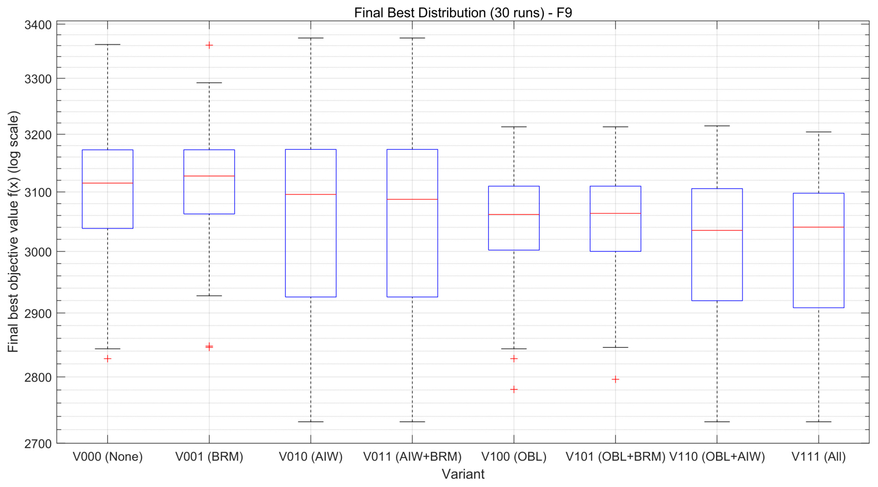
As shown in Figure 6 and

Table 2. Final best objective statistics and pairwise Wilcoxon test results across variants.

Number	Mean	Std	Median	Best	p-Value (vs. V111)
V000	3110.86	121	3115.07	2828.17	6.16 × 10−4 (Sig)
V001	3113.07	120	3127.21	2845.66	1.48 × 10−4 (Sig)
V010	3065.26	152	3095.68	2731.79	0.015 (Sig)
V011	3061.97	151	3087.37	2731.79	0.034 (Sig)
V100	3049.6	104	3061.66	2780.74	0.141 (NS)
V101	3050.14	102	3063.5	2796.26	0.072 (NS)
V110	3014.67	125	3034.98	2731.79	0.217 (NS)
V111	3011.28	123	3040.45	2731.79	-

Note: p-values are calculated using the Wilcoxon signed-rank test. “Sig” denotes significant difference (p < 0.05), “NS” denotes not significant.

, the statistical analysis confirms that the full framework (V111) significantly outperforms the baseline GOOSE (V000) and the boundary-only variant (V001) with p < 0.001, validating the overall effectiveness of the proposed improvements. The Adaptive Inertia Weight (AIW) mechanism is particularly influential, as evidenced by the significant difference between the single-module V010 and the full V111 (p = 0.015). While the OBL-based variants (V100) show a positive trend in mean reduction compared to the baseline, the statistical significance diminishes in the final convergence stage (p = 0.141), suggesting that OBL primarily accelerates early-stage exploration rather than final precision.

Regarding the comparison between the best dual-module variant (V110) and the full framework (V111), the p-value is 0.217 (>0.05). Although the addition of the Boundary Reflection Mechanism (BRM) does not yield a statistically significant improvement in the raw objective value for this specific benchmark, its retention is justified by engineering constraints. As indicated by the operational logs, V111 triggered boundary reflections in approximately 15% of the evaluations. Without BRM, these search agents would violate physical constraints. Thus, BRM serves a critical role in ensuring dimensional consistency and feasibility, safeguarding the optimization process against invalid parameter sets.

3. Result and Discussion

3.1. Test Functions and Parameter Settings

The performance of the proposed OGOOSE algorithm was evaluated using the CEC2017 benchmark suite. Specifically, four multimodal functions (F1–F4), four hybrid functions (F5–F8), and four composition functions (F9–F12) were selected, as summarized in

Table 3. Standard test functions.

Function Number	Function Name
F1	Shifted and Rotated Rosenbrock’s Function
F2	Shifted and Rotated Rastrigin’s Function
F3	Shifted and Rotated Expanded Scaffer’s F6 Function
F4	Shifted and Rotated Lunacek Bi-Rastrigin Function
F5	Hybrid Function 1 (N = 3)
F6	Hybrid Function 5 (N = 4)
F7	Hybrid Function 8 (N = 5)
F8	Hybrid Function 10 (N = 6)
F9	Composition Function 5 (N = 5)
F10	Composition Function 8 (N = 6)
F11	Composition Function 9 (N = 3)
F12	Composition Function 10 (N = 3)

. All functions were tested under identical experimental settings: dimension (dim = 50), population size (N = 30), iterations (T = 500), and independent runs (runs = 30). These parameter settings were strictly selected in accordance with the standard protocols of the CEC2017 competition [12] to ensure rigorous fairness and comparability with established literature.

Furthermore, the selection of these specific benchmark functions is well-suited to the proposed optimization framework. Since the ε-constraint method decomposes the multi-objective problem into a series of single-objective sub-problems, the solver’s performance on the challenging CEC2017 suite serves as a representative predictor of its efficacy in the engineering application. Specifically, the high-dimensional (d = 50) and multimodal functions are utilized to simulate the rugged, non-convex landscapes characteristic of robust Mean-CVaR objectives, acting as a necessary “stress test” to verify the algorithm’s global search capability.

The comparative algorithms selected for this study include the original GOOSE and two widely recognized swarm intelligence algorithms: the Harris Hawks Optimization (HHO) [13] and the Whale Optimization Algorithm (WOA) [14]. These methods were chosen as representative benchmarks from the recent decade due to their extensive citation and successful application in solving complex engineering problems, thus serving as a rigorous baseline for evaluating OGOOSE against established high-performance meta-heuristics. All four algorithms were executed 30 independent runs on each of the twelve CEC2017 benchmark functions F1–F12 to ensure experimental reliability and fair comparison. The performance results are summarized in

Table 4. Performance Results of Different Algorithms on Standard Test Functions.

Function Number	Indicator	GOOSE	OGOOSE	WOA	HHO
F1	Mean	1.512 × 103	7.746 × 102	2.942 × 103	1.213 × 103
	Std	8.414 × 102	8.563 × 101	8.909 × 102	1.879 × 102
	Mean(error)	1.212 × 103	4.746 × 102	2.642 × 103	9.134 × 102
F2	Mean	1.098 × 103	1.523 × 102	1.082 × 103	9.124 × 102
	Std	8.659 × 102	3.119 × 101	8.555 × 101	3.423 × 101
	Mean(error)	6.976 × 102	4.659 × 102	6.817 × 102	5.124 × 102
F3	Mean	6.790 × 102	6.662 × 102	6.960 × 102	6.774 × 102
	Std	8.015	3.776	8.972	4.896
	Mean(error)	1.790 × 102	1.662 × 102	1.960 × 102	1.774 × 102
F4	Mean	4.018 × 103	1.718 × 103	1.866 × 103	1.876 × 103
	Std	1.584 × 103	6.436 × 101	1.252 × 102	8.739 × 101
	Mean(error)	3.418 × 103	1.118 × 103	1.266 × 103	1.276 × 103
F5	Mean	4.004 × 103	1.455 × 103	5.992 × 103	2.137 × 103
	Std	1.791 × 103	4.578 × 101	1.539 × 103	3.603 × 102
	Mean(error)	3.004 × 103	4.548 × 102	4.992 × 103	1.137 × 103
F6	Mean	7.213 × 104	2.978 × 104	1.962 × 107	1.736 × 106
	Std	5.443 × 104	2.835 × 104	2.307 × 107	3.363 × 106
	Mean(error)	7.073 × 104	2.838 × 104	1.962 × 107	1.734 × 106
F7	Mean	2.883 × 106	1.735 × 106	4.870 × 107	8.616 × 106
	Std	1.941 × 106	1.407 × 106	3.395 × 107	8.236 × 106
	Mean(error)	2.881 × 106	1.733 × 106	4.870 × 107	8.614 × 106
F8	Mean	3.928 × 103	3.474 × 103	3.933 × 103	3.495 × 103
	Std	4.284 × 102	3.788 × 102	3.334 × 102	3.170 × 102
	Mean(error)	2.028 × 103	1.574 × 103	2.033 × 103	1.595 × 103
F9	Mean	3.835 × 103	3.264 × 103	4.416 × 103	3.485 × 103
	Std	7.341 × 102	3.877 × 101	3.525 × 102	1.038 × 102
	Mean(error)	1.435 × 103	8.636 × 102	2.016 × 103	1.085 × 103
F10	Mean	5.098 × 103	4.154 × 103	5.557 × 103	4.400 × 103
	Std	1.197 × 103	2.264 × 102	3.576 × 102	2.430 × 102
	Mean(error)	2.398 × 103	1.454 × 103	2.857 × 103	1.700 × 103
F11	Mean	7.121 × 103	6.951 × 103	9.097 × 103	6.737 × 103
	Std	8.633 × 102	1.010 × 103	1.627 × 103	8.384 × 102
	Mean(error)	4.321 × 103	4.151 × 103	6.297 × 103	3.937 × 103
F12	Mean	7.157 × 107	6.732 × 107	2.668 × 108	1.036 × 108
	Std	2.319 × 107	2.032 × 107	1.624 × 108	4.791 × 107
	Mean(error)	7.157 × 107	6.731 × 107	2.668 × 108	1.036 × 108

Bold formatting is used for the optimal results in Table 4 for emphasis.

. For each function, the “Mean” and “Std” columns report the mean and standard deviation of the final best-so-far objective value f(x) over the 30 runs, while the “Mean(error)” column reports the difference between this mean value and the corresponding “Optimal Value” listed in Table 3. All quantities are dimensionless and correspond to the raw objective values of the CEC2017 benchmarks.

As shown in Table 4, for the multimodal functions (F1–F4), the OGOOSE algorithm outperforms the other three algorithms in all three indicators—mean, standard deviation (Std), and mean error—indicating superior convergence accuracy and stability. For the hybrid functions (F5–F8), OGOOSE achieves the lowest mean error on all four functions and the lowest Std on three of them (HHO attains the smallest Std on F8). Its comparative advantage is particularly evident on F6 and F7, which exhibit large fluctuations. Regarding the composition functions (F9–F12), OGOOSE maintains a dominant position, achieving the best results on F9, F10, and F12. An exception is observed for F11 (Extended Weierstrass Function), where HHO exhibits slightly superior Mean and Mean(error) values. This can be attributed to the specific exploitative efficiency of HHO’s besieging mechanism on the Weierstrass landscape. However, considering the entire suite, OGOOSE outperforms all comparators on 11 out of 12 functions, demonstrating a significantly more robust overall capability in balancing exploration and exploitation.

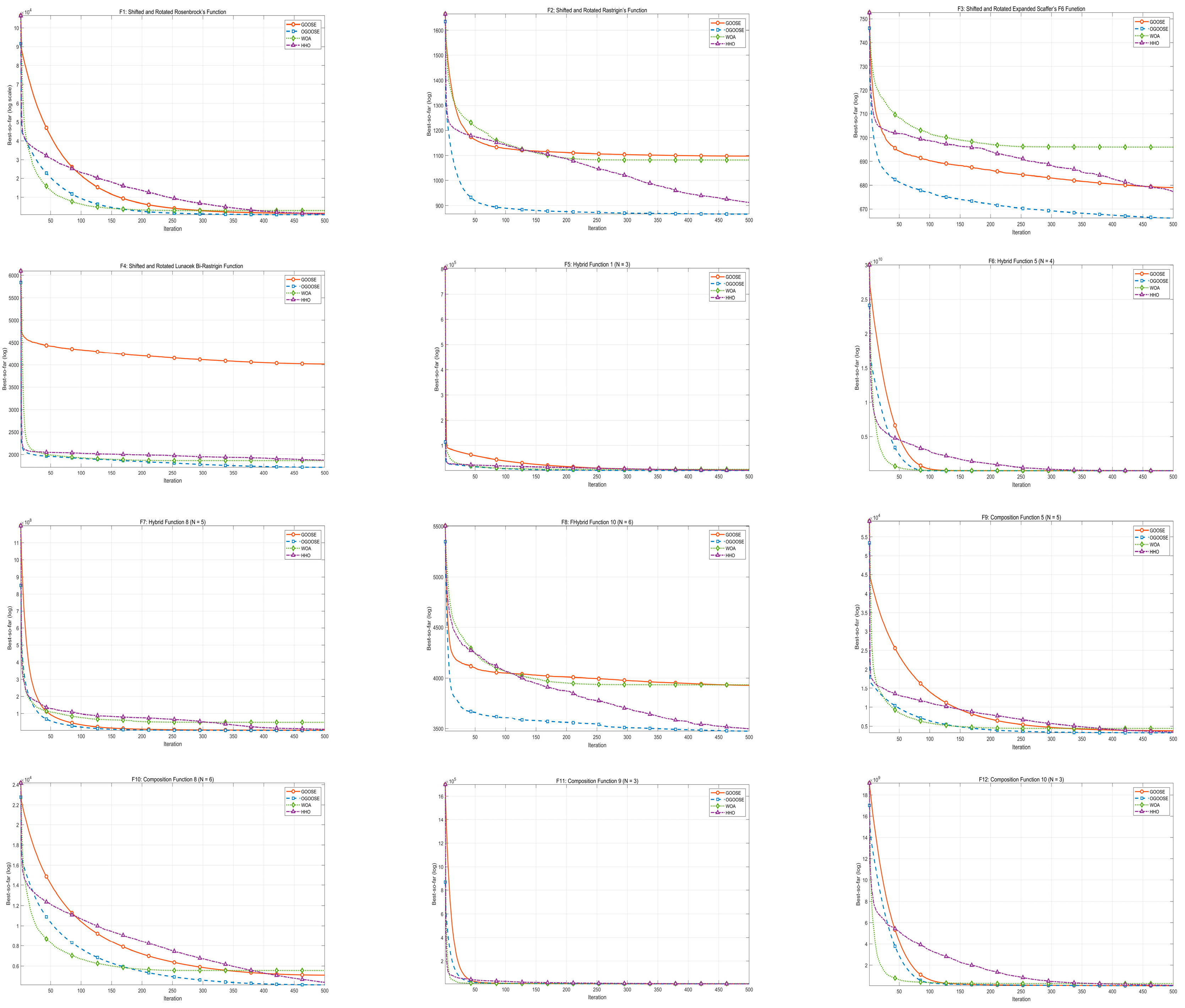
To further evaluate the convergence capability of the OGOOSE algorithm, Figure 7 illustrates the average convergence curves of the four algorithms across the 12 test functions. As observed, OGOOSE achieves faster convergence than the other algorithms on the majority of functions and establishes a clear lead in the early iterations. Furthermore, it attains the best final convergence accuracy on 11 out of 12 benchmarks (with F11 being the sole competitive case). These results clearly demonstrate the effectiveness of the three integrated modules in enhancing the overall performance of the OGOOSE algorithm.

3.2. Statistical Test Analysis

To assess whether the performance differences among the algorithms are statistically significant, we applied the non-parametric Friedman test to the “Mean(error)” values of the four algorithms over the twelve CEC2017 functions F1–F12 (treating the functions as blocks). At a significance level of 0.05, the Friedman test rejects the null hypothesis of equal performance, indicating significant overall differences. The corresponding average ranks are reported in

Table 5. Friedman Test and Ranking.

Algorithm Name	GOOSE	OGOOSE	WOA	HHO
AvgRank	2.917	1.083	3.750	2.250
Rank	3	1	4	2

, where “AvgRank” denotes the average rank of each algorithm across the 12 functions (lower values indicate better overall performance); since ranks are relative, no physical units are involved. OGOOSE obtains the best (lowest) average rank, followed by HHO, GOOSE and WOA.

Given this overall significance, a post hoc analysis was conducted using the Wilcoxon signed-rank test, again using the twelve functions as paired samples. OGOOSE was compared pairwise with each of the other three algorithms, and Holm’s step-down procedure was used to adjust the p-values for multiple comparisons. The raw and adjusted p-values, together with the comparison symbols, are listed in

Table 6. Wilcoxon Test Results and Holm Correction for Algorithm Comparisons.

Algorithm Name	Wilcoxon Test p-Value	p-Value After Holm Correction	Symbol	Result
OGOOSEvsGOOSE	0.000488	0.00293	+	Significant
OGOOSEvsWOA	0.000488	0.00293	+	Significant
OGOOSEvsHHO	0.00488	0.0146	+	Significant

. In this table, the symbol “+” indicates that OGOOSE is significantly better than the compared algorithm at the 0.05 significance level; the test statistics and p-values are dimensionless.

These statistical results indicate that, on the CEC2017 benchmark set, OGOOSE achieves a significantly better overall performance than the other three algorithms.

3.3. Key Decisions and Feasible Region in Multi-Objective Optimization

In this study, the decision vector X consists of two core variables: the step coefficient ($x_1$) and the ore-drawing step ($x_2$) [15]. These variables jointly determine the spatial rhythm and intensity of the blasting, ore extraction, and mixing processes. The variable search space is confined to an engineeringly feasible and representative range: the step coefficient $x_1$ and ore-drawing step $x_2$ are confined to the intervals [1.32, 1.43] and [4.30, 4.60], respectively, aligning with the validated operational bounds reported by [16]. This configuration covers the typical on-site candidate schemes while avoiding infeasible or meaningless searches.

Under this framework, the evaluation objectives consist of four interrelated indicators: unit ore production cost (C), safety risk (R), ore recovery rate (H), and dilution rate (P). The decision vector influences these indicators through two primary mechanisms: (1) Geometric configuration, which modifies the spatial shape of the extraction body and the ore–waste interface, thereby directly affecting recovery and dilution; and (2) Process intensity, which alters the density of the drilling network, indirectly influencing cost and safety risk. Crucially, the relationship between these objectives is fundamentally asymmetrical, as a small increase in dilution or risk disproportionately impacts profitability compared to a marginal decrease in cost. Environmental and geological parameters other than the decision variables—such as rock mass density, extracted ore volume within the evaluation period, and interface orientation or offset—are subjected to bounded perturbations that introduce operational asymmetry in the uncertainty modeling process, but are not included in the decision-level optimization.

In this study, these uncertain parameters are modeled as bounded random perturbations around their nominal engineering values. Specifically, each uncertain quantity ${\mathsf{\zeta }}_k$ is assumed to lie in a symmetric interval $[{\mathsf{\zeta }}_k^0(1-{\mathsf{\delta }}_k),\hspace{0.17em}{\mathsf{\zeta }}_k^0(1 +{ \mathsf{\delta }}_k\left)\right]$, where ${\mathsf{\zeta }}_k^0$ denotes the nominal value, and $\mathsf{\delta }$ is a prescribed relative variation level. In the experiments, $\mathsf{\delta }$ is set to 0.10 for all uncertain parameters, representing a moderate ±10% deviation that is commonly used in engineering sensitivity studies to mimic medium-scale geological and operational fluctuations. A scenario s corresponds to one joint realization ${\mathsf{\zeta }}^{\left(s\right)} = \left({\mathsf{\zeta }}_1^{\left(s\right)},\dots ,{\mathsf{\zeta }}_K^{\left(s\right)}\right)$ obtained by independent Monte Carlo sampling from these bounded intervals. The S = 40 scenarios used in the robust evaluation are generated once with fixed random seeds and are shared by all algorithms and all ε-subproblems, so that the comparison is carried out under identical stochastic conditions.

Subsequently, through a multi-scenario “Expectation + CVaR” robust evaluation framework combined with the ε-constraint method [17], the aforementioned multi-objective problem is transformed into a series of subproblems with a unified primary objective and explicit constraints, thereby ensuring fair and comparable algorithmic performance evaluation.

3.4. Continuously Differentiable and Dimensionally Consistent Model Based on “Ellipsoid–Plane” Geometry

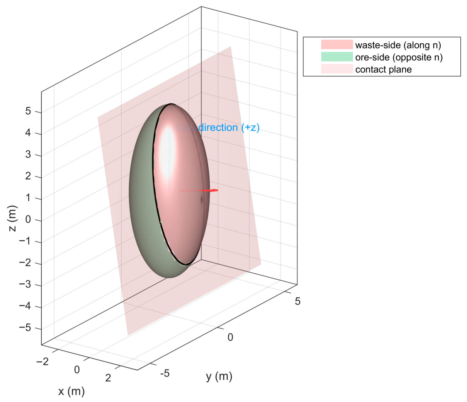
To ensure that the calculations of ore recovery rate and dilution rate not only align with engineering physical intuition but also avoid reliance on arbitrarily assigned exponential functions or unstable proportional relationships, this study adopts a concise and robust geometric surrogate model, as illustrated in Figure 8. The core idea is that the ore extraction body is approximated as a triaxial ellipsoid, which can be conceptualized as an “ore extraction cloud” centered at the extraction point and extending variably along the longitudinal, lateral, and vertical directions. This ideal ellipsoidal geometry symbolizes the structural symmetry of the resource extraction process. As the ore caving step x₂ increases, the dimensions along all three axes expand synchronously, reflecting the principle that larger steps correspond to a wider influence range. The mathematical representation is given in Equations (24) and (25):

$$\begin{array}{c}{\displaystyle \frac{x^2}{{\mathrm{a}}^2}} + {\displaystyle \frac{{\mathrm{y}}^2}{{\mathrm{b}}^2}} + {\displaystyle \frac{{\mathrm{z}}^2}{{\mathrm{c}}^2}} \le 1\end{array}$$

(24)

The semi-axes vary linearly with the ore caving step x₂, as expressed by:

$$\begin{array}{l}\left\{\begin{array}{c}\mathrm{a} = {\mathrm{a}}_0 + { \mathrm{k}}_{\mathrm{a}}{\mathrm{x}}_{\mathrm{2}},\\ \mathrm{b} ={ \mathrm{b}}_0 +{ \mathrm{k}}_{\mathrm{b}}{\mathrm{x}}_2,\\ \mathrm{c} ={ \mathrm{c}}_0 + {\mathrm{k}}_{\mathrm{c}}{\mathrm{x}}_{\mathrm{2}}\end{array}\right.\end{array}$$

(25)

where a, b, c are the semi-axes of the ellipsoid (units: m) corresponding to the longitudinal (x), lateral (y), and vertical (z), respectively; a₀, b₀, c₀ are the base semi-axis values (units: m) representing the ellipsoid size under the minimum working space, with values of 3 m, 1.0 m, and 1.2 m, respectively; K_a, k_b, k_c are the linear amplification coefficients representing the sensitivity of each direction to the ore caving step, with values of 0.3, 0.15, and 0.18, respectively.

The ore-waste mixing boundary is approximated as a plane. Its normal direction is determined by the flow direction azimuth, and its position (offset relative to the extraction center) is jointly adjusted by the ore caving step and step coefficient. The intervention and offset of this plane relative to the symmetrical ellipsoid volume introduce geometric asymmetry into the system, leading directly to dilution and loss. This plane divides the ellipsoid volume in 3D space into ore and waste rock parts, thereby determining the recovery and dilution ratios [18]. During the calculation, the ellipsoid is normalized to a unit sphere by scaling in all directions, and a consistent mapping is applied to this plane. At this point, recovery and dilution only depend on the “dimensionless distance from the plane to the sphere center”, with the calculation formula shown in Equation (26).

$$\begin{array}{c}\left\{\begin{array}{l}\mathit{n} · \mathrm{r}=\mathrm{d}\\ \mathsf{\zeta }={\displaystyle \frac{\mathrm{d}}{\Vert {\mathrm{A}}^{\mathrm{T}}\mathit{n}\Vert }}\end{array}\right.\end{array}$$

(26)

where $\mathit{n}$ is the unit normal vector of the interface, pointing to the waste rock side; $\mathrm{r}$ is the position vector of any point in space; $\mathrm{d}$ is the directed distance from the interface to the coordinate origin; $\mathsf{\zeta }$ is the normalized distance parameter; $\mathrm{A}$ is the diagonal matrix of the ellipsoid semi-axes.

Once the unit sphere is intersected by the plane, the dilution rate is equal to the volume fraction of the spherical cap on the waste-rock side. For a unit sphere, the cross-section at height z has area:

$$A\left(z\right) = \mathsf{\pi }(1-z^2)$$

(27)

When the normalized distance satisfies −1 < $\mathsf{\zeta }$ < 1, the plane z = $\mathsf{\zeta }$ cuts off a spherical cap above the plane. The volume of this cap is:

$$V_{\mathrm{cap}}(\mathsf{\zeta }) ={\int }_{\mathsf{\zeta }}^1\mathsf{\pi }(1-z^2)\hspace{0.17em}\mathit{dz} = \mathsf{\pi }\left({\displaystyle \frac{2}{3}}-\mathsf{\zeta } + {\displaystyle \frac{{\mathsf{\zeta } }^3}{3}}\right)$$

(28)

The total volume of the unit sphere is $(V_{\mathrm{sphere}} = {\displaystyle \frac{4}{3}}\mathsf{\pi })$. Therefore, the volume fraction on one side of the plane is:

$${\mathsf{\varphi }}_{\mathrm{cap}}(\mathsf{\zeta }) = {\displaystyle \frac{V_{\mathrm{cap}}\left(\mathsf{\zeta }\right)}{V_{\mathrm{sphere}}}} =\left\{\begin{array}{ll}0,& \mathsf{\zeta } \ge 1,\\ {\displaystyle \frac{(1-\mathsf{\zeta }{)}^2(2 + \mathsf{\zeta })}{4}},& -1< \mathsf{\zeta } <1,\\ 1,& \mathsf{\zeta } \le -1\end{array}\right.$$

(29)

In this study, the volume fraction ${\mathsf{\varphi }}_{\mathrm{cap}}\left(\mathsf{\zeta }\right)$ is explicitly mapped to the Dilution Rate (P), while its complement corresponds to the Ore Recovery Rate $(H = 1- P)$. By construction, both quantities are bounded within [0, 1] and satisfy the physical limiting cases: P = 0 (implying H = 1, i.e., full recovery with no dilution) when the plane lies entirely on the ore side (ζ ≥ 1), and P = 1 (full dilution, zero recovery) when it is outside on the waste-rock side (ζ ≤ −1).

In sublevel caving, the ore–waste interface is locally irregular owing to fragmentation and particle interlocking. In the present work, the ellipsoid–plane geometry is adopted as a macroscopic surrogate for the cumulative drawbody, in line with previously reported ellipsoid-based draw models and shape analyses under similar mining conditions [1,18]. The semi-axes a, b and c and the position of the interface plane are chosen within the range reported in these studies, so that the resulting draw ellipsoid has comparable dimensions and dilution evolution.

Within this framework, the surrogate is intended to describe the dominant dependence of dilution and recovery on the decision variables (x₁, x₂), while small-scale geometric roughness that cannot be controlled at the planning stage is intentionally smoothed out. From the optimization perspective, such an approximation mainly influences the absolute levels of dilution and recovery but preserves their relative variation with respect to (x₁, x₂), because the same surrogate structure is applied uniformly to all candidate solutions in the ε-constraint search. The ellipsoid–plane model is therefore suitable for analyzing and comparing draw strategies at the strategic planning scale considered in this study.

3.5. Multi-Objective ε-Constraint Robust Optimization Based on the OGOOSE Algorithm

Within the robust multi-objective optimization framework, this study considers four evaluation indicators—Cost (C), Risk (R), Recovery (H), and Dilution (P)—and employs the ε-constraint method to decompose the original problem. The robust objective values ($\widehat{C}$, $\widehat{R}$, $\widehat{H}$, $\widehat{P}$) are formulated using the Mean-CVaR criterion (Equation 30) to rigorously quantify uncertainty:

$$\left\{\begin{array}{ll}\widehat{C}& = \mathrm{E}[C] + {\mathsf{\lambda }}_{\mathrm{c}}\cdot {\mathrm{CVaR}}_{\mathsf{\beta }}(C),\\ \widehat{R}& = \mathrm{E}[R] + {\mathsf{\lambda }}_{\mathrm{r}}\cdot {\mathrm{CVaR}}_{\mathsf{\beta }}(R),\\ \widehat{H}& = -\mathrm{E}[H] + {\mathsf{\lambda }}_{\mathrm{h}}\cdot {\mathrm{CVaR}}_{\mathsf{\beta }}(-H),\\ \widehat{P}& = \mathrm{E}[P] +{ \mathsf{\lambda }}_{\mathrm{p}}\cdot {\mathrm{CVaR}}_{\mathsf{\beta }}(P).\end{array}\right.$$

(30)

where $\mathrm{E}[·]$ denotes the expectation over the S stochastic scenarios, ${\mathrm{CVaR}}_{\mathsf{\beta }}(·)$ is the Conditional Value at Risk at confidence level β, and ${\mathsf{\lambda }}_{\mathrm{c}}$, ${\mathsf{\lambda }}_{\mathrm{r}}$, ${\mathsf{\lambda }}_{\mathrm{h}}$ and ${\mathsf{\lambda }}_{\mathrm{p}}$ ≥ 0 are the risk-aversion coefficients controlling the trade-off between mean performance and tail risk for cost, risk, recovery and dilution, respectively. The resulting aggregated quantities $\widehat{C}$, $\widehat{R}$, $\widehat{H}$, $\widehat{P}$ are the robust objective values used in the ε-constraint formulation.

To balance statistical validity with the feasibility of computationally expensive optimization [19], the hyperparameters are configured as follows. The scenario count is set to S = 40, which satisfies the heuristic threshold (N ≥ 30) for the Central Limit Theorem and provides a sufficient statistical basis to approximate the risk distribution without incurring the prohibitive cost of very large sample sets [20]. The CVaR confidence level is fixed at (β = 0.90) in order to target the mitigation of top-decile (10%) adverse outcomes; this level avoids the excessive conservatism associated with β = 0.99 while still capturing the most relevant tail risks for mining production. The tail sample size is chosen as m = 5 (slightly larger than the theoretical value S(1 − β) = 4) as a smoothing device to stabilize the empirical CVaR estimate against individual outliers.

For a given decision vector x, the robust objectives in Equation (30) are evaluated on the fixed scenario set $\{1,\dots , S\}$. Let $\left\{C^{\left(s\right)}\right(x){\}}_{s = 1}^S$ denote the scenario-wise unit cost values and $\left\{C_{\left(j\right)}\right(x){\}}_{j = 1}^S$ their order statistics in non-decreasing order. The expectation term is approximated by the sample mean, as shown in Equation (31):

$$\hat{E}[C\left]\right(x)={\displaystyle \frac{1}{S}}\sum _{s=1}^S{C}^{\left(s\right)}(x)$$

(31)

And the empirical CVaR (Conditional Value-at-Risk) at confidence level β is computed as the average of the worst m scenarios, which is given in Equation (32):

$$\widehat{\mathrm{CVa}{R}_{\mathsf{\beta }}}(C\left)\right(x)={\displaystyle \frac{1}{m}}\sum _{j=S-m+1}^S{C}_{\left(j\right)}(x)$$

(32)

where m = 5 corresponds to a tail fraction slightly larger than the theoretical value S(1−β) = 4 in order to smooth the estimator for the finite-sample case. The same procedure is applied to the other objectives R H, P, with the convention that CVaR is taken on the transformed quantity -H for the recovery-related term.

To ensure fairness and reproducibility, the scenario set and ε-grid are constructed once and consistently shared across OGOOSE and the comparative algorithms (GOOSE, WOA, HHO). Fixed random seeds were assigned to both the scenario generation and the optimization processes to guarantee identical stochastic conditions.

To guarantee that the ϵ-constraints focus on the operationally relevant ‘Knee Region’ rather than spanning irrelevant extremes, a Percentile-Based Grid Strategy is employed. First, a preliminary random sampling (N_sample = 60) is conducted within the decision space. The constraint bounds [ε_min,ε_max] for Risk and Dilution are then determined by the 20th and 70th percentiles of the sample objective distributions, respectively. Subsequently, a grid density of q = 3 is defined for both dimensions, generating a focused 3 × 3 matrix of sub-problems. The thresholds are generated linearly within these percentile bounds:

$${\mathsf{\epsilon }}_{k , j} ={ P}_{20\%}(f_k) + {\displaystyle \frac{j}{q-1}} \times (P_{70\%}(f_k) -{ P}_{20\%}(f_k\left)\right) j = 0,\dots ,q-1$$

(33)

where P_x% denotes the x-th percentile. This strategic grid confinement effectively directs computational resources toward the most operationally viable trade-off regions, thereby avoiding computational waste on extreme outlier scenarios.

For each subproblem, a unified penalty function is employed to scalarize the formulation, with robust cost minimization ($\widehat{C}$) serving as the core objective. A standard ‘Big-M’ penalty coefficient (M = 106) is applied to enforce strict feasibility regarding the robust constraints, as expressed in Equation (34):

$${\mathrm{f}}_{\mathsf{\epsilon }}(x) =\widehat{ C}(x) + \mathrm{M}\cdot \left[\max (0,\widehat{R}(x)-{\mathsf{\epsilon }}_{\mathrm{R}}) + \max (0,\widehat{P}(x) -{ \mathsf{\epsilon }}_{\mathrm{P}}) + \max (0,\widehat{H}(x)-{\mathsf{\epsilon }}_{\mathrm{H}})\right]$$

(34)

where $x$ is the decision variable vector; ${\mathsf{\epsilon }}_{\mathrm{R}}$,${ \mathsf{\epsilon }}_{\mathrm{P}}$,${ \mathsf{\epsilon }}_{\mathrm{H}}$ represent the threshold constraints.

This comparative study is specifically designed to evaluate the search efficiency of OGOOSE as a scalarizing solver within the ε-constraint framework. Consequently, state-of-the-art single-objective meta-heuristics (GOOSE, WOA, HHO) serve as the primary baselines. This focused comparison allows for the rigorous isolation of the algorithmic enhancements (OBL, AIW, BRM) applied to the search engine, avoiding confounding factors associated with different multi-objective frameworks. Furthermore, given the computationally expensive nature of the robust Mean-CVaR simulation, the adopted ε-constraint approach offers a pragmatic engineering advantage by enabling a targeted search for preferred “knee-point” solutions, presenting a more computationally efficient alternative to the exhaustive Pareto front approximation typically required by dominance-based or decomposition-based evolutionary algorithms (e.g., NSGA-II [21] or MOEA/D [22,23]).

Table 7. Comparative performance of four algorithms under the robust ε-constraint multi-objective optimization framework.

mean_C	mean_R	mean_P	mean_H	IGD_raw	Mean Time_s
112.290	0.007852	0.289465	0.7105	0.002835	75.93
112.286	0.007854	0.289469	0.7105	0.001312	72.34
112.287	0.007855	0.289469	0.7105	0.001066	71.90
112.286	0.007855	0.289469	0.7105	0.001309	177.92

summarizes the robust ε-constraint multi-objective optimization performance of the four algorithms under the same computational budget. Here “mean_C” denotes the average unit production cost [CNY/t]; “mean_R” denotes the average robust risk index (dimensionless); “mean_P” and “mean_H” denote the average dilution rate and recovery rate, respectively (fractions in [0, 1]); “IGD_raw” is the Inverted Generational Distance in the original objective space (dimensionless); and “Mean Time_s” is the average CPU time in seconds per ε-subproblem. All statistics in Table 7 are computed as mean values over 10 independent runs of each algorithm under the same scenario set and ε-grid. The computational experiments were conducted on a standard computing environment equipped with an Intel Core i7-8565U processor (1.80 GHz) and 8 GB RAM. The average runtime of 75.93 s per run (with S = 40 scenarios) confirms that the robust simulation is computationally viable even on modest hardware. The complete statistical evaluation of the 3 × 3 grid (totaling 90 independent runs) requires approximately 2 h, representing a highly efficient workflow for strategic mine design.

From an engineering viewpoint, the four algorithms produce almost identical unit costs and recovery rates: the unit cost (mean_C) is approximately 112.29 CNY/t for all methods, and the average recovery (mean_H) is 0.7105 (71.05%). Against this essentially equal cost–recovery background, OGOOSE attains the lowest average risk and dilution, with mean_R = 0.007852 compared with 0.007854–0.007855 for the other algorithms, and mean_P = 0.289465 compared with 0.289469. Although these numerical differences are small, they are systematic: under the same computational budget and almost identical economic and recovery performance, OGOOSE always achieves the lowest risk–dilution levels among the four methods. This consistent pattern indicates that OGOOSE offers a more favorable risk–dilution profile without any noticeable penalty in cost or recovery.

To contextualize this performance, the recent literature defines a clear performance spectrum for sublevel caving in similar inclined orebodies. On one end, experimental studies such as Tao et al. (2019) [24] indicate that under conventional operational conditions targeting high recovery, dilution rates often exceed 30%. On the other end, state-of-the-art structural parameter optimization [25] has established a rigorous experimental baseline of approximately 27.5% under ideal controlled conditions. The 28.95% achieved by OGOOSE successfully lands within this high-performance interval. It significantly outperforms the typical operational norm (>30%) and remains highly competitive with the ideal experimental baseline (27.5%). Crucially, this result is derived under stochastic geological perturbations, demonstrating that OGOOSE effectively stabilizes product quality against uncertainty, preventing the performance deterioration often observed in traditional deterministic designs.

The IGD_raw (calculated in the original objective space) serves as a metric to evaluate both the convergence proximity and the distributional diversity of the solution set relative to the reference Pareto front. As detailed in Table 7, WOA achieves the lowest IGD_raw (0.001066), followed by HHO and GOOSE, whereas OGOOSE records a higher value of 0.002835. This apparent statistical discrepancy requires interpretation within the specific engineering context. Mathematically, IGD penalizes algorithms that fail to uniformly cover the entire extent of the reference front. WOA’s superior IGD score implies it generates a broader spread of solutions, likely populating extreme regions of the trade-off surface (e.g., scenarios with prohibitive costs for marginal risk reduction). However, in the context of robust mining optimization, operational performance indicators (Cost, Risk, Dilution) take precedence over the geometrical uniformity of the solution set. From a practical decision-making standpoint, an algorithm is preferred if it converges reliably to the ‘Knee Region’—the segment of the Pareto front offering the most advantageous trade-off—rather than expending computational resources to map impractical extremes. As evidenced by the first-order engineering metrics, OGOOSE achieves the lowest Risk (0.007852) and Dilution (0.289465) among all comparators, while maintaining competitive Cost and Recovery levels. This indicates that OGOOSE exhibits a ‘focused convergence’ behavior, concentrating its search capability within the most operationally viable zone. Consequently, despite a higher IGD value attributed to reduced spread, OGOOSE is deemed more practically valuable for this high-stakes application, as it delivers superior solutions in the specific metrics that directly govern mine profitability and safety”.

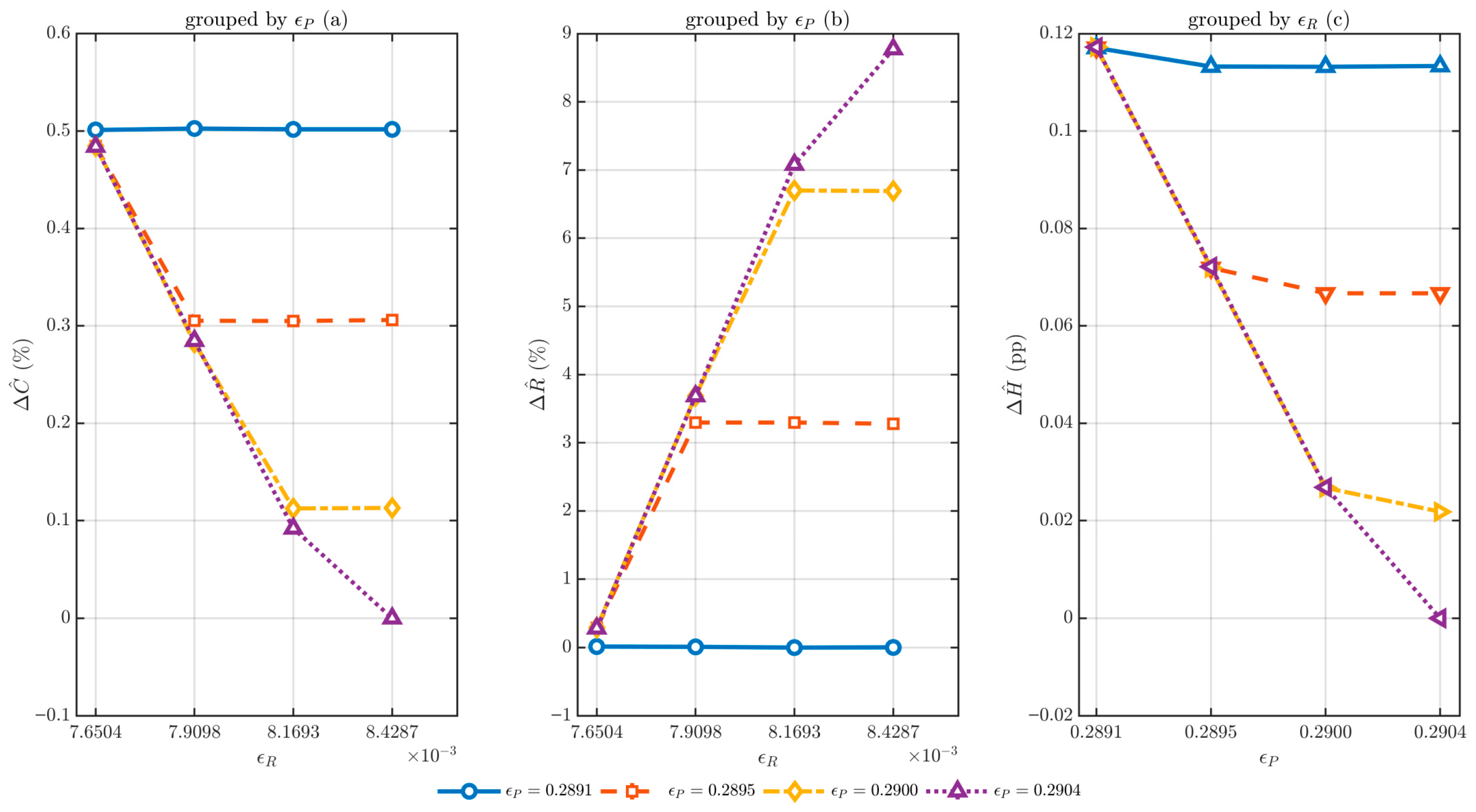
Figure 9 illustrates the trade-off between benefit and cost resulting from threshold adjustments. In the cost and risk dimensions (Figure 9a,b), when the dilution threshold is relatively strict (small εP), relaxing the risk threshold εR has only a marginal effect on the robust cost, while the corresponding risk increase remains minor. As εP is gradually relaxed, the variation in the curves becomes more pronounced: Δ$\widehat{R}$(%) exhibits a steady decline with increasing εR, whereas Δ$\widehat{R}$(%) rises concurrently at an accelerating rate. This result suggests that under loose dilution constraints, moderate relaxation of the risk threshold can yield a certain cost reduction, though at the expense of a higher risk level. The response pattern of the recovery rate (Figure 9c) follows a similar trend. With εR fixed, ΔH decreases monotonically as εP increases; the decline is more pronounced at higher εR levels but nearly insensitive at lower ones. This indicates that simultaneous relaxation of risk and dilution constraints produces a compounding adverse effect on recovery rate; hence, significant simultaneous adjustments of both thresholds should be avoided in practice. By integrating the results of the three subfigures, a more economical and robust operational range can be identified—corresponding to a combination of moderate εR and appropriate εP. Within this range, risk growth remains within acceptable limits, losses in recovery and grade are contained, and cost reduction has not yet reached diminishing marginal returns.

In engineering scenarios prioritizing safety and quality control, OGOOSE better embodies the principle of stable and reliable operation. Without increasing cost or excessively compromising recovery, it consistently reduces both risk and dilution rates, and this advantage remains stable across multiple ε combinations. This consistent performance suggests that during long-term operation and multi-shift fluctuations, OGOOSE can more effectively maintain the enterprise’s safety margins and product quality thresholds. Although its computational time is not the shortest, it remains within an acceptable range, and its overall cost-effectiveness makes it a preferred default solver for engineering applications.

4. Conclusions

This study proposes OGOOSE, a robust multi-objective optimization framework specifically designed to address systemic operational asymmetry in sublevel caving. The key conclusions are drawn as follows:

(1)

Algorithmic Efficacy: The integration of Opposition-Based Learning (OBL), Adaptive Inertia Weight (AIW), and Boundary Reflection (BRM) significantly enhances the baseline algorithm. Ablation studies confirm that OBL and AIW are the primary drivers for balancing exploration and exploitation, while BRM is essential for enforcing feasibility constraints with negligible computational overhead.

(2)

Benchmark Superiority: OGOOSE achieves the lowest Friedman rank on the CEC2017 suite, statistically outperforming HHO, WOA, and GOOSE. While it may not consistently yield the smallest IGD metric due to its focused search within the Pareto “knee region,” it demonstrates superior stability and robustness in complex multimodal landscapes.

(3)

Engineering Performance: In the sublevel caving case study, OGOOSE attains the lowest average risk (0.0078) and dilution rate (28.95%) among all comparators, without compromising robust cost or recovery. With a runtime only 5.6% higher than the fastest baseline, it offers a pragmatic trade-off between solution quality and computational efficiency.

(4)

Operational Insight: The ε-sensitivity analysis identifies a distinct “knee-point” trade-off region. The results suggest that a strategy combining moderate risk acceptance with strict dilution control maximizes operational value. Conversely, the simultaneous relaxation of both risk and dilution constraints incurs compounding penalties on recovery and should be avoided.

(5)

Limitations: The current framework relies on an idealized ellipsoid-plane surrogate and empirically selected hyperparameters. Additionally, the ε-constraint formulation, while effective for finding knee points, requires careful grid resolution tuning to avoid missing critical trade-off regions. Future work will prioritize the integration of site-specific geological data, the development of adaptive parameter tuning schemes, and the extension of this robust methodology to other mining contexts.

References

1. Soleimani Bafghi, S.A.; Nasab, H.H.; Fakhrzad, M.B.; Soltani, R.; Bafghi, A.Y. A multi-objective Fuzzy Robust Optimization model for open-pit mine planning under uncertainty. Soft Comput. 2025, 29, 213–235. [Google Scholar] [CrossRef] [Scilit]
2. Hu, J.; Zhang, Y.; Yu, Z.; Huang, M.; Huang, M.; Dong, J.; Lin, J. Study on morphological evolution of IEZ and model refinement in natural caving. J. Cent. South Univ. (Sci. Technol.) 2025, 56, 2440−2449. [Google Scholar]
3. Tang, A.; Han, T.; Xu, D.; Xie, L. Path Planning Method Based on Chaotic Sparrow Search Algorithm. J. Comput. Appl. 2021, 41, 2128–2136. [Google Scholar]
4. Ding, W.; Su, X.; Liao, S.; Tang, Q.; Yang, J. Optimization of Photovoltaic Energy Storage Capacity Allocation Based on Harris Hawk Optimization Algorithm. Electron. Des. Eng. 2024, 32, 96–101. [Google Scholar]
5. Wang, H.; Zhang, Y. Multi-Policy Improved HHO and Its Application in Intelligent Scheduling. Comput. Meas. Control. 2024, 1–10. Available online: https://link.cnki.net/urlid/11.4762.TP.20240614.1342.029 (accessed on 4 November 2025).
6. Li, Y.; Lin, X.; Liu, J. Multi-Strategy Integrated Harris Hawk Algorithm to Solve Global Optimization Problems. Oper. Res. Manag. Sci. 2024, 33, 28–34. [Google Scholar]
7. Hamad, R.K.; Rashid, T.A. GOOSE algorithm: A powerful optimization tool for real-world engineering challenges and beyond. Evol. Syst. 2024, 15, 1249–1274. [Google Scholar] [CrossRef] [Scilit]
8. Tizhoosh, H.R. Opposition-based learning: A new scheme for machine intelligence. In Proceedings of the International Conference on Computational Intelligence for Modelling, Control and Automation and International Conference on Intelligent Agents, Web Technologies and Internet Commerce (CIMCA-IAWTIC’06), Vienna, Austria, 28–30 November 2005; IEEE: New York, NY, USA, 2005; Volume 1, pp. 695–701. [Google Scholar]
9. Kirkpatrick, S.; Gelatt, C.D., Jr.; Vecchi, M.P. Optimization by simulated annealing. Science 1983, 220, 671–680. [Google Scholar] [CrossRef] [Scilit]
10. May, R.M. Simple mathematical models with very complicated dynamics. Nature 1976, 261, 459–467. [Google Scholar] [CrossRef] [Scilit]
11. Sampson, J.R. Adaptation in natural and artificial systems (John H. Holland). SIAM Rev. 1976, 18, 529–530. [Google Scholar] [CrossRef] [Scilit]
12. Wu, G.; Mallipeddi, R.; Suganthan, P.N. Problem Definitions and Evaluation Criteria for the CEC 2017 Competition on Constrained Real-Parameter Optimization; Technical Report 9; National University of Defense Technology: Changsha, China; Kyungpook National University: Daegu, Republic of Korea; Nanyang Technological University: Singapore, 2017; p. 2017. [Google Scholar]
13. Heidari, A.A.; Mirjalili, S.; Faris, H.; Aljarah, I.; Mafarja, M.; Chen, H. Harris hawks optimization: Algorithm and applications. Future Gener. Comput. Syst. 2019, 97, 849–872. [Google Scholar] [CrossRef] [Scilit]
14. Mirjalili, S.; Lewis, A. The whale optimization algorithm. Adv. Eng. Softw. 2016, 95, 51–67. [Google Scholar] [CrossRef] [Scilit]
15. Sun, H.; Jin, A.B.; Gao, Y.T.; Meng, X.Q. Study on the shape of the isolated extraction zone under different end wall angles and determination of the optimal blast ring spacing. Chin. J. Eng. 2016, 38, 2095–2099. [Google Scholar] [CrossRef]
16. An, L.; Xu, S.; Li, Y.H.; Peng, J.Y. Optimization of blast ring spacing in caving method based on multi-method combination. Chin. J. Rock Mech. Eng. 2013, 32, 754–759. Available online: https://rockmech.whrsm.ac.cn/CN/Y2013/V32/I4/754 (accessed on 4 November 2025).
17. Haimes, Y. On a Bicriterion Formulation of the Problems of Integrated System Identification and System Optimization. IEEE Trans. Syst. Man Cybern. 1971, 3, 296–297. [Google Scholar]
18. Tian, D.; Shi, H.Y.; Fu, E.J.; Niu, G.X. Study on the relationship between coal drawing step and drawing rate based on the ellipsoid theory. Coal Sci. Technol. 2015, 43, 51–53, 143. [Google Scholar] [CrossRef]
19. Chugh, T.; Sindhya, K.; Hakanen, J.; Miettinen, K. A survey on handling computationally expensive multiobjective optimization problems with evolutionary algorithms. Soft Comput. 2019, 23, 3137–3166. [Google Scholar] [CrossRef] [Scilit]
20. Pan, L.; He, C.; Tian, Y.; Wang, H.; Zhang, X.; Jin, Y. A classification-based surrogate-assisted evolutionary algorithm for expensive many-objective optimization. IEEE Trans. Evol. Comput. 2018, 23, 74–88. [Google Scholar] [CrossRef] [Scilit]
21. Deb, K.; Pratap, A.; Agarwal, S.; Meyarivan, T. A fast and elitist multiobjective genetic algorithm: NSGA-II. IEEE Trans. Evol. Comput. 2002, 6, 182–197. [Google Scholar] [CrossRef] [Scilit]
22. Zhang, Q.; Li, H. MOEA/D: A multiobjective evolutionary algorithm based on decomposition. IEEE Trans. Evol. Comput. 2007, 11, 712–731. [Google Scholar] [CrossRef] [Scilit]
23. Zhou, A.; Zhang, Q.; Zhang, G. A multiobjective evolutionary algorithm based on decomposition and probability model. In Proceedings of the 2012 IEEE Congress on Evolutionary Computation, Brisbane, Australia, 10–15 June 2012; IEEE: New York, NY, USA, 2012. [Google Scholar]
24. Tao, G.; Yang, J.; Ren, F.; Zhang, X. Experimental study on guided flow drawing in medium-thick inclined ore body. J. Min. Saf. Eng. 2019, 36, 59–64. [Google Scholar]
25. Zhou, B.; Elmo, D.; Chen, X.; Wu, Y.; Li, G. Optimization of Structural Parameters in Sublevel Caving: Insights from Ore-Waste Rock Movement Patterns. Min. Metall. Explor. 2025, 42, 1677–1691. [Google Scholar] [CrossRef] [Scilit]
Figure 1. Scatter plot of the initial population distribution. The axes Z1 and Z2 correspond to the first two decision variables (dimensionless) of the search space.
Symmetry 18 00254 g001
Figure 2. Empirical Cumulative Distribution Function (ECDF) of the initialization error. The horizontal axis represents the initialization error value (dimensionless), and the vertical axis represents the cumulative probability.
Symmetry 18 00254 g002
Figure 4. Flow chart for the algorithm.
Symmetry 18 00254 g004
Figure 5. Convergence curves of the eight ablation variants (V000–V111) of GOOSE on the CEC2017 test function F9 (Composition Function 7, dim = 50). The horizontal axis denotes the iteration index t, and the vertical axis denotes the best-so-far objective value f(x) on a logarithmic scale (dimensionless raw function value). Solid curves show the mean over 30 independent runs; light shaded bands for V000, V110 and V111 indicate ±1 standard deviation. Variant codes follow Table 1, where V000 is the original GOOSE (no module), V111 is the full configuration (OBL + AIW + BRM), and the remaining codes correspond to single-and dual-module combinations.
Symmetry 18 00254 g005
Figure 6. Log-scale boxplots of the final best objective value f(x) over 30 independent runs for each ablation variant (V000–V111) under the same experimental setting as in Figure 5. The vertical axis shows the raw (dimensionless) objective value f(x) on a logarithmic scale. Boxplots summarize the distribution of the final results (median, interquartile range, whiskers and outliers), where the box represents the interquartile range, the red line inside each box indicates the median, and the “+” symbols denote outliers.
Symmetry 18 00254 g006
Figure 3. Schematic diagram of the symmetric boundary reflection mechanism. The horizontal axis (X) denotes the candidate solution position before correction, and the vertical axis (Y) denotes the mapped position after reflection (both are dimensionless).
Symmetry 18 00254 g003
Figure 7. Mean convergence curves of GOOSE, OGOOSE, WOA and HHO on the twelve CEC2017 benchmark functions F1–F12. Each panel corresponds to one test function, whose identifier and name are given in the panel title. The horizontal axis shows the iteration index t, and the vertical axis shows the best-so-far objective value f(x) on a logarithmic scale; values are averaged over 30 independent runs and are dimensionless. The four algorithms are represented by consistent color and marker coding in all panels.
Symmetry 18 00254 g007
Figure 8. Three-dimensional draw ellipsoid and contact plane. The semi-transparent plane represents the ore-waste mixing boundary whose unit normal vector n (red arrow) points toward the waste-rock side. The pink region of the ellipsoid corresponds to the waste-rock side (along n ), and the green region corresponds to the ore side (opposite n ).
Symmetry 18 00254 g008
Figure 9. Sensitivity of the robust cost, risk and recovery to the risk threshold ε_R and the dilution threshold ε_P. Panels (ac) show the normalized changes Δ C ^ (%), Δ R ^ (%) and ΔH (percentage points) as functions of ε_R or ε_P. Here Δ C ^ (%) and Δ R ^ (%) denote the percentage increase in robust cost and risk relative to the best values C_min and R_min observed over the entire ε-grid, i.e., C_min = min C ^ (ε_R, ε_P) and R_min = min R ^ (ε_R, ε_P), while ΔH(pp) denotes the percentage-point increase in recovery relative to the worst recovery H_min = min H(ε_R, ε_P). Colors and markers identify different fixed levels of ε_P (or ε_R) and are consistent across the three panels.
Symmetry 18 00254 g009