Formal Equivalence Between Maxwell Equations and the de Broglie–Bohm Theory for Two-Dimensional Optical Microcavities

Abstract

We analyze the formal equivalence between the electromagnetic energy conservation law derived from Maxwell’s equations in an optical microcavity and the conservation of a probability fluid associated with the de Broglie–Bohm theory for an effective massive particle describing a photon in this cavity. This work is part of a critical analysis of recent experiments by Sharoglazova et al. carried out with a view to refuting the de Broglie–Bohm theory. Furthermore, the consequences of our analysis for microphotonics go far beyond these experiments. In particular, extensions that take into account photon spin and stochastic aspects associated with radiative or absorption losses are considered. From the point of view of symmetries and probability current, here the effective photon behaves like a spin-1/2 particle.

1. Introduction

The de Broglie–Bohm pilot wave theory, i.e., Bohmian mechanics [1,2,3,4], is originally an alternative interpretation of quantum mechanics that preserves the notion of classical determinism and the notion of trajectories for particles.

It can be rigorously demonstrated that, given certain statistical assumptions about the so-called quantum equilibrium regime, Bohmian theory is capable of reproducing the entirety of quantum mechanics, at least in the non-relativistic regime. In particular, probabilistic predictions and quantum measurement theory can be encompassed and fully justified within a Bohmian framework [4,5,6].

However, there is no consensus regarding relativistic quantum theories, including quantum field theories (QFTs) or even quantum optics. Among the various approaches that have been attempted in QFT, we mention Bohm’s initial work based on a functional representation of the quantum electromagnetic field coupled to a (non-relativistic) description of fermions treated as particles [3,7,8]. We also mention attempts to develop Bohmian quantum electrodynamics (QED) for the Dirac equation based on the old ideas of an infinite sea of negative-energy particles [3,9,10]. Finally, we mention works inspired by Bell’s research, which introduces stochastic elements into the Bohmian approach in order to take into account the creation and annihilation of particles in QFT [11,12,13,14].

Beyond these fundamental and interpretative questions, there is no doubt that Bohmian formalism, based on a hydrodynamic representation known as Madelung’s representation of wave Equations (Schrödinger, Klein–Gordon, Dirac), is an interesting tool for describing wave propagation phenomena in complex environments. In optics, and particularly in nano/microphotonics, a Bohmian analogy of wave propagation is certainly possible, even in the classical regime based on pure Maxwell equations. In such a theory, the speed of the Bohmian fluid must intuitively be related to the propagation of the energy fluid deduced from Maxwell’s equations via Poynting’s theorem (in general, the inferred velocity is less than the speed limit of light c and corresponds to an effective particle with a variable non-zero mass). This is what we will show below.

More precisely, in this paper, we propose such a Bohmian hydrodynamic formulation for a classical electromagnetic field propagating in a planar optical microcavity. This work is initially motivated by recent results published by Sharoglazova et al. [15,16] (see also [17,18,19,20]) concerning the Bohmian velocity in a microcavity, but the consequences go far beyond that work and open up new perspectives in nano-optics. Based on an experiment involving structured waveguides in a planar optical microcavity, these authors sought to demonstrate an inconsistency in Bohmian theory in the evanescent wave regime using an optical analog of the tunnel effect. We recently proposed a clear refutation of this claim [21] based principally on the existence of radiative leaks neglected in the authors’ analysis, which allows us to unambiguously determine a Bohmian velocity even in their experiment. We stress that in [21], we highlighted a second effect linked to the finite duration of the excitation pulses, which in itself is sufficient to invalidate the results of [15] and save Bohmian mechanics from refutation. However, as the optical response is dominated by radiative leakage, we will not consider it further here. However, underlying this work is the assumption that a coherent Bohmian formalism exists in such a microcavity. In the model published to date, we start from a formal analogy between the wave equations in the microcavity and a particle with effective mass $m_{eff}$ due to the particular paraxial regime used. This strongly motivates an equivalence between the wave equations of the electromagnetic field and the non-relativistic Schrödinger equation for a massive particle. However, the Bohmian theory assumed in these works is not exactly deduced from Maxwell’s equations, and the link between energy propagation and Bohmian propagation is not firmly established. We emphasize that this in no way invalidates previous analyses made to account for observations, as the analysis based on the paraxial and Gaussian optical regime (which assumes that the wave vector of light is primarily oriented along an optical axis [22]) is sufficiently well established at such a phenomenological level. In other words, readers wishing to find a refutation of claim [15] can simply read the self-sufficient work [21]. However, in a second step, this strongly suggests a more detailed theoretical analysis of this type of paraxial analogy and the equivalence between Bohmian dynamics and energy transport in a 2D microcavity. Furthermore, given the importance of the problem more generally for the study of optical microcavities, we propose here to justify the existence of such a Bohmian model for a 2D optical analogy.

In this context, it is essential to note that de Broglie, guided by Einstein’s work, had suggested as early as 1924-25 [23,24] (i.e., before the discovery of Schrödinger’s equation) that the speed of photons is given by the ratio between the Poynting vector $\mathbf{S}=\mathbf{E}\times \mathbf{B}$, which defines the local energy flux, and the local energy density $u={\displaystyle \frac{{\mathbf{E}}^2+{\mathbf{B}}^2}{2}}$:

$$\begin{array}{c}\hfill \mathbf{v}(\mathbf{x},t)={\displaystyle \frac{\mathbf{S}(\mathbf{x},t)}{u(\mathbf{x},t)}}=2{\displaystyle \frac{\mathbf{E}(\mathbf{x},t)\times \mathbf{B}(\mathbf{x},t)}{{\mathbf{E}}^2(\mathbf{x},t)+{\mathbf{B}}^2(\mathbf{x},t)}}\end{array}$$

(1)

where $\mathbf{E}(\mathbf{x},t)$ and $\mathbf{B}(\mathbf{x},t)$ are, respectively, the electric and magnetic field vector at point $\mathbf{x}$ and time t obeying Maxwell equations. Such ideas were also introduced by Slater [25].

The motivation for this formula is, of course, the local law of conservation of energy ${\partial }_{t}u=-\mathbf{\nabla }·\mathbf{S}$. Similarly, in the case of the Schrödinger equation for a single particle of mass m, according to Bohmian mechanics, we can define a local velocity for the particle using the ratio between the probability current $\mathbf{J}(\mathbf{x},t)={\displaystyle \frac{1}{m}}\mathrm{Im}[{\Psi }^{*}(\mathbf{x},t)\mathbf{\nabla }\Psi (\mathbf{x},t)]$ and the local probability density $\rho (\mathbf{x},t)={\Psi }^{*}(\mathbf{x},t)\Psi (\mathbf{x},t)$, which gives the de Broglie–Bohm guidance formula:

$$\begin{array}{c}\hfill {\mathbf{v}}_{dBB}(\mathbf{x},t)={\displaystyle \frac{\mathbf{J}(\mathbf{x},t)}{\rho (\mathbf{x},t)}}={\displaystyle \frac{1}{m}}\mathrm{Im}\left[{\displaystyle \frac{\mathbf{\nabla }\Psi (\mathbf{x},t)}{\Psi (\mathbf{x},t)}}\right]\end{array}$$

(2)

where $\Psi (\mathbf{x},t)$ is the wavefunction obeing the nonrelativistic Schrödinger equation.

Here again, an obvious motivation for this formula lies in the law of local conservation ${\partial }_t\rho =-\mathbf{\nabla }·\mathbf{J}$. However, it is important to note some fundamental differences between Maxwell’s case and Schrödinger’s:

(i) First of all, in the case of Schrödinger’s equation, we are dealing with the current and density of a probability fluid, whereas in Maxwell’s case, we are dealing with an energy fluid. This is central from a physical point of view. Moreover, from a relativistic point of view, the energy fluid does not define a current four-vector but is part of an energy-momentum tensor $T^{\mu \nu }$. The velocity obtained therefore cannot have fundamental relativistic validity. In contrast, in the case of Schrödinger’s equation, the guiding formula can easily be generalized to the Dirac or Klein–Gordon equation, where the current and density form a current four-vector, which by definition is written as $J^{\mu }:=[\rho ,\mathbf{J}]$, with the correct Lorentz covariant meaning (note, however, that for the Klein–Gordon case, the current $J^{\mu }$ is not always time-like [4]).

In this work, where we are only interested in hydrodynamic optical analogies for an optical microcavity, we will not seek to preserve the relativistic covariance of the problem, and we can ignore this issue.

(ii) Another fundamental difference is, of course, that Maxwell’s theory is based on real electric and magnetic fields, whereas Schrödinger’s wave function is a complex field. In the regime under consideration, we will show that the introduction of a complex electromagnetic field is naturally required if we assume a light source that randomly emits pulses of an identical nature and form but shifted in time by a statistically distributed variable delay. Furthermore, the transition from a field with multiple E and B components to a single wave function will also be justified by the symmetries and approximations of the problem under consideration.

(iii) A final important difference between Maxwell’s equations and Schrödinger’s equation concerns linearity and the absence of a source term in the latter. In particular, the conservation law for electromagnetic energy generally contains a source term associated with the electric current interacting with the electric field: ${\partial }_{t}u=-\mathbf{\nabla }·\mathbf{S}-{\mathbf{J}}_e·\mathbf{E}$. Such a source term is absent from the probabilistic conservation law in the Schrödinger equation because the number of particles is conserved in the non-relativistic regime. However, this difference disappears in the relativistic regime, particularly in QED, and Bohmian models that take this fact into account have been developed. We will not have to consider this problem in full generality because we will limit ourselves to linear optical media where electric currents are linked to local polarization. Note, however, that including loss and absorption by the optical medium requires such a stochastic approach as discussed below.

Of course, the ideas developed in this work are inspired by these pioneering studies, but also by recent and equally important work that emphasizes the relevance and importance of Bohmian analogies in describing light propagation in paraxial regimes [26] and in connection with so-called weak measurements of photon trajectories in free space [27,28]. The originality of our work therefore lies more in the application of these concepts to a 2D system. We emphasize that our results are clearly consistent with these important studies [26,27,28].

The structure of the paper is as follows: In Section 2, we provide a detailed formulation of Maxwell’s equations in terms of complex electromagnetic fields. In particular, we introduce the Poynting vector and the energy density associated with this complex field, and we discuss the issue of absorption. In Section 3, we justify the emergence of an effective Schrödinger equation for the Maxwell field in an ideal planar microcavity. These results are then extended to the case of a lossy cavity in Section 4. In both Section 3 and Section 4, we develop a Bohmian analogy and demonstrate that the in-plane velocity of the energy fluid within the cavity corresponds precisely to the Bohmian velocity derived from the Schrödinger equation. Section 4 also discusses possible extensions of the model including stochasticity or spin. In particular we show that the photon formally behaves like a spin-1/2 particle despite the obvious differences in symmetry between a boson and a fermion. The respective roles of radiative and absorption losses are compared, and the implications for a probabilistic interpretation of the effective Bohmian fluid are discussed in relation to stochasticity. Finally, in Section 5, we revisit the discussion surrounding the claims made in [15], in light of our previous comment [21] and the present work. We conclude by summarizing the implications of our findings for integrated optics and Bohmian mechanics.

2. The Poynting Theorem for Complex Effective Electromagnetic Fields

We start from Maxwell’s equations in the vacuum and we add electric current ${\mathbf{J}}_{\mathbf{e}}={\partial }_t\mathbf{P}+\mathbf{\nabla }\times \mathbf{M}$ and charge ${\rho }_e=-\mathbf{\nabla }·\mathbf{P}$ distributions corresponding to the presence of electric polarization $\mathbf{P}$ and magnetic polarization $\mathbf{M}$:

$$\begin{array}{cc}\hfill \mathbf{\nabla }\times \mathbf{E}=-{\partial }_t\mathbf{B},& \mathbf{\nabla }·\mathbf{B}=0\\ \hfill \mathbf{\nabla }\times \mathbf{B}={\partial }_t\mathbf{E}+{\partial }_t\mathbf{P}+\mathbf{\nabla }\times \mathbf{M},& \mathbf{\nabla }·\mathbf{E}=-\mathbf{\nabla }·\mathbf{P}\end{array}$$

(3)

In a linear regime (i.e., dielectric and magnetic medium), we assume the following constitutive relations in order to satisfy Kramers–Kronig causal constraints (for a review see [29,30]):

$$\begin{array}{c}\hfill \mathbf{P}(\mathbf{x},t)={\int }_0^{+\infty }d\tau {\chi }_E(\mathbf{x},\tau )\mathbf{E}(\mathbf{x},t-\tau )\\ \hfill \mathbf{M}(\mathbf{x},t)={\int }_0^{+\infty }d\tau {\chi }_M(\mathbf{x},\tau )\mathbf{B}(\mathbf{x},t-\tau )\end{array}$$

(4)

with ${\chi }_{E,M}(\mathbf{x},\tau )$ linear susceptibilities depending on a time delay $\tau$ associated with dispersion and dissipation (note that for simplicity, here we assume spatially local media).

At this point, we introduce statistical assumptions and assume that the electromagnetic state is described by a linear superposition of pulses, such that for each pulse we use a Fourier decomposition of the type

$$\begin{array}{c}\hfill {\mathbf{E}}_{\delta }(\mathbf{x},t)={\int }_0^{+\infty }d\omega {\mathbf{E}}_{\omega }\left(\mathbf{x}\right)e^{-i(\omega t+\delta (\omega \left)\right)}+cc.\end{array}$$

(5)

and similarly for the magnetic induction field. Basically, we have in fact introduced a phase delay $\delta \left(\omega \right)$, which is assumed to vary randomly from one pulse to another. For greater precision, we limit ourselves to the hypothesis $\delta \left(\omega \right)={\delta }_0$ so that we can write

$$\begin{array}{c}\hfill {\mathbf{E}}_{\delta }(\mathbf{x},t)=\mathcal{E}(\mathbf{x},t)e^{i{\delta }_0}+cc.\end{array}$$

(6)

with $\mathcal{E}(\mathbf{x},t)={\int }_0^{+\infty }d\omega {\mathbf{E}}_{\omega }\left(\mathbf{x}\right)e^{-i\omega t}$ a complex electric field (and similarly for the magnetic induction field) [29,30].

Using this assumption about random phases, it is easy to convince oneself that each of Maxwell’s equations must be satisfied for complex fields $\mathcal{E}$, $\mathcal{B}$, $\mathcal{P}$, and $\mathcal{M}$, i.e.,

$$\begin{array}{cc}\hfill \mathbf{\nabla }\times \mathcal{E}=-{\partial }_t\mathcal{B}& ,\mathbf{\nabla }·\mathcal{B}=0\\ \hfill \mathbf{\nabla }\times \mathcal{B}={\partial }_t\mathcal{E}+{\partial }_t\mathcal{P}+\mathbf{\nabla }\times \mathcal{M}& ,\mathbf{\nabla }·\mathcal{E}=-\mathbf{\nabla }·\mathcal{P}\end{array}$$

(7)

and the linear equations comprising Equation (4) are left unchanged, with real fields replaced by complex fields.

In this new framework, we recall that according to Poynting’s theorem derived from Equation (3), we have

$$\begin{array}{c}\hfill \mathbf{E}{\partial }_t\mathbf{D}+\mathbf{H}{\partial }_t\mathbf{B}=-\mathbf{\nabla }·[\mathbf{E}\times \mathbf{H}]\end{array}$$

(8)

where we have introduced the usual fields, $\mathbf{D}=\mathbf{E}+\mathbf{P}$ (electric displacement) and $\mathbf{H}=\mathbf{B}-\mathbf{M}$ (magnetic field). In this formula, the Poynting vector associated with the local energy flux is defined by $\mathbf{S}=\mathbf{E}\times \mathbf{H}$. We can easily extend Poynting’s theorem to the complex Maxwell field directly from Equation (7)

$$\begin{array}{c}\hfill 2\mathrm{Re}[{\mathcal{E}}^{*}{\partial }_t\mathcal{D}+{\mathcal{H}}^{*}{\partial }_t\mathcal{B}]=-\mathbf{\nabla }·2\mathrm{Re}[{\mathcal{E}}^{*}\times \mathcal{H}]\end{array}$$

(9)

Alternatively, we can obtain this formula by introducing a probability distribution $P\left(\delta \right)$ for the random phase $\delta :={\delta }_0$ and defining the mean $\langle A_{\delta }(\mathbf{x},t)\rangle =\int d\delta P\left(\delta \right)A_{\delta }(\mathbf{x},t)$. We thus obtain $\langle {\mathbf{E}}_{\delta }{\partial }_t{\mathbf{D}}_{\delta }+{\mathbf{H}}_{\delta }{\partial }_t{\mathbf{B}}_{\delta }\rangle =2\mathrm{Re}[{\mathcal{E}}^{*}{\partial }_t\mathcal{D}+{\mathcal{H}}^{*}{\partial }_t\mathcal{B}]$ by averaging Equation (8), and similarly $\langle {\mathbf{S}}_{\delta }(\mathbf{x},t)\rangle =2\mathrm{Re}[{\mathcal{E}}^{*}\times \mathcal{H}]:=\mathcal{S}$, which leads once again to Equation (9).

In order to be more specific about the type of model considered here, we introduce the electric permittivity ${\epsilon }_{\omega }$ and the magnetic permeability ${\mu }_{\omega }$ defined by relations

$$\begin{array}{c}\hfill {\epsilon }_{\omega }\left(\mathbf{x}\right)=1+{\int }_0^{+\infty }d\tau {\chi }_E(\mathbf{x},\tau )e^{i\omega \tau }\\ \hfill {\mu }_{\omega }\left(\mathbf{x}\right)={\displaystyle \frac{1}{1-{\int }_0^{+\infty }d\tau {\chi }_M(\mathbf{x},\tau )e^{i\omega \tau }}}\end{array}$$

(10)

and following Landau and Lifschitz in their Electrodynamics of Continuous Media [29], we work in the weakly dispersive regime around a mean frequency ${\omega }_0$. According to these authors, writing $\mathcal{E}(\mathbf{x},t)=\tilde{\mathcal{E}}(\mathbf{x},t)e^{-i{\omega }_{0}t}$ where the envelope field $\tilde{\mathcal{E}}$ varies slowly compared to $e^{-i{\omega }_{0}t}$, we deduce the following at the first-order approximation:

$$\begin{array}{c}\hfill {\mathcal{E}}^{*}{\partial }_t\mathcal{D}\simeq -i{\omega }_0{\epsilon }_{{\omega }_0}{\left|\mathcal{E}\right|}^2+{\displaystyle \frac{d\left(\omega {\epsilon }_{\omega }\right)}{d\omega }}{|}_{{\omega }_0}{\tilde{\mathcal{E}}}^{*}{\partial }_t\tilde{\mathcal{E}}\end{array}$$

(11)

which allows us to rewrite Poynting’s theorem Equation (9) in the approximate form:

$$\begin{array}{c}\hfill {\displaystyle \frac{d\left(\omega {\epsilon }_{\omega }^{\prime }\right)}{d\omega }}{|}_{{\omega }_0}{\partial }_t{\left|\mathcal{E}\right|}^2+{\displaystyle \frac{d\left(\omega {\mu }_{\omega }^{\prime }\right)}{d\omega }}{|}_{{\omega }_0}{\partial }_t{\left|\mathcal{H}\right|}^2\\ \hfill \simeq -\mathbf{\nabla }·2\mathrm{Re}[{\mathcal{E}}^{*}\times \mathcal{H}]-2{\omega }_0{\epsilon }_{{\omega }_0}^{″}{\left|\mathcal{E}\right|}^2-2{\omega }_0{\mu }_{{\omega }_0}^{″}{\left|\mathcal{H}\right|}^2\\ \hfill -2\mathrm{Im}\left[{\tilde{\mathcal{E}}}^{*}{\partial }_t\tilde{\mathcal{E}}\right]{\displaystyle \frac{d\left(\omega {\epsilon }_{\omega }^{″}\right)}{d\omega }}{{|}_{{\omega }_0}-2\mathrm{Im}\left[{\tilde{\mathcal{H}}}^{*}{\partial }_t\tilde{\mathcal{H}}\right]{\displaystyle \frac{d\left(\omega {\mu }_{\omega }^{″}\right)}{d\omega }}|}_{{\omega }_0}\end{array}$$

(12)

where ${\epsilon }_{\omega }^{\prime }=\mathrm{Re}\left[{\epsilon }_{\omega }\right]$, ${\epsilon }_{\omega }^{″}=\mathrm{Im}\left[{\epsilon }_{\omega }\right]$ and similarly for ${\mu }_{\omega }$.

This equation can be interpreted physically. On the left-hand side, the time derivative of the well-known electromagnetic energy density $\mathcal{U}=\langle u_{\delta }\rangle ={\displaystyle \frac{d\left(\omega {\epsilon }_{\omega }^{\prime }\right)}{d\omega }}{|}_{{\omega }_0}{\left|\mathcal{E}\right|}^2+{\displaystyle \frac{d\left(\omega {\mu }_{\omega }^{\prime }\right)}{d\omega }}{|}_{{\omega }_0}{\left|\mathcal{H}\right|}^2$ appears. On the right-hand side, apart from the usual divergence term involving the Poynting vector $\mathcal{S}$, there are terms related to the dissipation of the polarized medium $-2{\omega }_0{\epsilon }_{{\omega }_0}^{″}{\left|\mathcal{E}\right|}^2-2{\omega }_0{\mu }_{{\omega }_0}^{″}{\left|\mathcal{H}\right|}^2$. Since the imaginary parts ${\epsilon }_{\omega }^{″},{\mu }_{\omega }^{″}$ are always positive by virtue of the Kramers–Kronig relations for a dissipative system, this corresponds to absorption by the polarizable medium. The last terms on the right-hand side are more difficult to interpret and are considered negligible by Landau and Lifschitz [29].

We point out that our derivation of Poynting’s theorem for a polarizable medium is more general than those usually given in the literature, because we use ensemble averages in the delay space $\delta$ rather than time averages. This allows us to introduce complex electromagnetic fields and retain time dependencies in our expressions.

To conclude this first part, we have derived Poynting’s theorem

$$\begin{array}{c}\hfill {\partial }_t\mathcal{U}=-\mathbf{\nabla }·\mathcal{S}-\mathcal{W}\end{array}$$

(13)

with

$$\begin{array}{c}\hfill \mathcal{U}=\langle u_{\delta }\rangle ={\displaystyle \frac{d\left(\omega {\epsilon }_{\omega }^{\prime }\right)}{d\omega }}{|}_{{\omega }_0}{\left|\mathcal{E}\right|}^2+{\displaystyle \frac{d\left(\omega {\mu }_{\omega }^{\prime }\right)}{d\omega }}{|}_{{\omega }_0}{\left|\mathcal{H}\right|}^2\\ \hfill \mathcal{S}=\langle {\mathbf{S}}_{\delta }\rangle =2\mathrm{Re}[{\mathcal{E}}^{*}\times \mathcal{H}]\end{array}$$

(14)

and a dissipation term $\mathcal{W}=2{\omega }_0{\epsilon }_{{\omega }_0}^{″}{\left|\mathcal{E}\right|}^2+2{\omega }_0{\mu }_{{\omega }_0}^{″}{\left|\mathcal{H}\right|}^2$. This allows us to introduce a velocity for the energy flow with the definition:

$$\begin{array}{c}\hfill \mathbf{v}(\mathbf{x},t)={\displaystyle \frac{\mathcal{S}(\mathbf{x},t)}{\mathcal{U}(\mathbf{x},t)}}={\displaystyle \frac{\langle {\mathbf{S}}_{\delta }(\mathbf{x},t)\rangle }{\langle u_{\delta }(\mathbf{x},t)\rangle }}={\displaystyle \frac{2\mathrm{Re}[{\mathcal{E}}^{*}\times \mathcal{H}]}{\frac{d\left(\omega {\epsilon }_{\omega }^{\prime }\right)}{d\omega }{|}_{{\omega }_0}{\left|\mathcal{E}\right|}^2+\frac{d\left(\omega {\mu }_{\omega }^{\prime }\right)}{d\omega }{|}_{{\omega }_0}{\left|\mathcal{H}\right|}^2}}\end{array}$$

(15)

We should note that in the absence of a dielectric medium (i.e., if ${\epsilon }_{\omega }=1$), we obtain the formula

$$\begin{array}{c}\hfill \mathbf{v}(\mathbf{x},t)={\displaystyle \frac{2\mathrm{Re}[{\mathcal{E}}^{*}\times \mathcal{B}]}{{\left|\mathcal{E}\right|}^2+{\left|\mathcal{B}\right|}^2}}\end{array}$$

(16)

This formula, based on an ensemble average, was already postulated on physical grounds by de Broglie in 1925 [24] for their pilot-wave theory of photons instead of the overly general formula Equation (1).

More precisely, the role of a temporal average (rather than an ensemble average such as that used in the present work) was emphasized by de Broglie. Indeed, it should be noted that at the time of de Broglie, it was already known from classical electrodynamics that an optical detector had to respond to a signal proportional to ${\mathbf{E}}^2(\mathbf{x},t)$. The fact of involving a time, or, better, an ensemble average allows us to obtain a detected intensity proportional to ${\left|\mathcal{E}(\mathbf{x},t)\right|}^2$, which closely resembles a Born rule for a probability of presence in non-relativistic quantum mechanics. In particular, for stationary light, the detected flux is independent of time, which is not the case for ${\mathbf{E}}^2(\mathbf{x},t)$.

For de Broglie [24], this was a sign that the true photonic field underlying their pilot-wave theory was complex and not real, thereby anticipating Schrodinger’s equation, with its complex wave function, and Born’s statistical rule discovered in 1926. Note that the justification for a complex electromagnetic field for the photon is rigorously obtained in QED, and we will briefly discuss this point in Section 4.4.

3. Bohmian Formalism for an Ideal Two-Dimensional Optical Microcavity

3.1. Derivation from Maxwell’s Equation

Having developed a hydrodynamic representation for the energy fluid based on a complex electromagnetic field, this suggests, by direct analogy with what has been done for the Schrödinger or Dirac equation, defining a velocity for a light particle using Equation (16). However, at this stage, we note that the presence of a loss term $\mathcal{W}$ is at odds with a purely deterministic approach. Indeed, the presence of $\mathcal{W}(\mathbf{x},t)$ implies that the trajectories of light particles can in some cases be interrupted at space-time point $x^{\mu }:=[t,\mathbf{x}]$ due to absorption by the dissipative medium.

Moreover, it is possible to develop an approach similar to that of Bell and taken up by Tumulka et al. to produce a stochastic Bohmian version of QFT [11,12,13,14] (this will be briefly discussed in the next section). In the present section we will neglect losses and absorption and suppose a purely deterministic hydrodynamic (Bohmian) picture

In this paper, we consider a simplified model of a planar optical cavity used in [15]. First, we neglect dispersion and dissipation and consider only a dielectric medium with constant permittivity $\epsilon$ located between two parallel perfect plane mirrors separated by a distance $D_0$ along the z axis. Moreover, one of the mirrors is weakly structured, and we consider that the distance between the mirrors changes as $D(x,y)=D_0+\delta D(x,y)$ where $\left|\delta D(x,y)\right|/D_0\ll 1$. The wave equations for the electromagnetic fields in the cavity are then written as

$$\begin{array}{c}\hfill [\epsilon {\partial }_t^2-{\mathbf{\nabla }}^2]\left(\begin{array}{c}\mathcal{E}\\ \mathcal{B}\end{array}\right)=0.\end{array}$$

(17)

Furthermore, we work in the paraxial regime and assume that the electromagnetic field is mainly in the $x-y$ plane parallel to the mirror, while propagation occurs essentially along the z axis. If we work at a fixed frequency $\omega$, this generates a standing wave along the z axis. To simplify, we write $\mathcal{E}=\widehat{\mathbf{e}}\Phi (x,y,z)e^{-i\omega t}$, with $\widehat{\mathbf{e}}$ being a unit constant polarization vector parallel to the $x-y$ plane. The vector is assumed to be real, i.e., $\widehat{\mathbf{e}}\in {\mathbb{R}}^3$. Note that the theory can easily be extended to more complex cases with two wave functions ${\Phi }_{\pm }$ forming a spinor. We will briefly analyze this possibility at the end of Section 4. The wave Equation (17) reads $\epsilon {\omega }^2\Phi +{\partial }_z^2\Phi +{\mathbf{\nabla }}_{\left|\right|}^2\Phi =0$ (where ${\mathbf{\nabla }}_{\left|\right|}$ is the gradient operator in the $x-y$ plane) with the approximate solution

$$\begin{array}{c}\hfill \Phi (x,y,z)={\Psi }_E(x,y)f_{x,y}\left(z\right)\end{array}$$

(18)

assuming

$$\begin{array}{c}\hfill f_{x,y}\left(z\right)=sin({\displaystyle \frac{q\pi }{D(x,y)}}z)\end{array}$$

(19)

with $q\in \mathbb{N}$. The z-component of the wave vector reads $k_z(x,y)={\displaystyle \frac{q\pi }{D(x,y)}}\simeq {\displaystyle \frac{q\pi }{D_0}}-{\displaystyle \frac{q\pi \delta D(x,y)}{D_0^2}}$. In particular, for $\delta D=0$ and $\Psi$ as a constant, we have the dispersion relation $\epsilon {\omega }^2={\left({\displaystyle \frac{q\pi }{D_0}}\right)}^2$. This allows us to introduce an effective mass $m={\displaystyle \frac{1}{\sqrt{\epsilon }}}{\displaystyle \frac{q\pi }{D_0}}$, and we write $k_z(x,y)=\sqrt{\epsilon }(m+V(x,y))$, where $V(x,y)=-{\displaystyle \frac{1}{\sqrt{\epsilon }}}{\displaystyle \frac{q\pi \delta D(x,y)}{D_0^2}}$ is an effective potential for the in-plane motion ($\left|V\right|/m\ll 1$). We are considering frequency $\omega$ close to m and write $\omega =m+E$ (i.e., $E/m\ll 1$). The wave equation becomes

$$\begin{array}{c}\hfill [\epsilon {(m+E)}^2-\epsilon {(m+V(x,y))}^2+{\mathbf{\nabla }}_{\left|\right|}^2]{\Psi }_E(x,y)=0\end{array}$$

(20)

and in the ‘nonrelativistic’ approximation $E/m\ll 1$, $\left|V\right|/m\ll 1$ this leads to the time-independent effective Schrödinger equation:

$$\begin{array}{c}\hfill [2\epsilon m(E-V(x,y))+{\mathbf{\nabla }}_{\left|\right|}^2]\Psi (x,y)\simeq 0.\end{array}$$

(21)

We can easily extend the solution to time-dependent problems by constructing wave packets $\Psi (x,y,t)=\int dE{\Psi }_E(x,y)e^{-iEt}$ such that $E/m\ll 1$. We then have the time-dependent Schrödinger equation

$$\begin{array}{c}\hfill i{\partial }_t\Psi (x,y,t)=-{\displaystyle \frac{{\mathbf{\nabla }}_{\left|\right|}^2}{2\epsilon m}}\Psi (x,y,t)+V(x,y)\Psi (x,y,t)\end{array}$$

(22)

and we note that including the prefactor $e^{-imt}$ would just add a mass term $m\Psi$ to the right hand side of the equation. We stress that we did not consider the role of the transversality condition $\mathbf{\nabla }·\mathcal{D}=\epsilon \mathbf{\nabla }·\mathcal{E}=0$ derived from Maxwell’s equations for the dielectric medium with constant permittivity. We will back to this issue in Section 4.

This Schrödinger equation clearly motivates a 2D Bohmian analogy with the inplane guidance formula for the fluid velocity:

$$\begin{array}{c}\hfill {\mathbf{v}}_{dBB,\left|\right|}(x,y,t)={\displaystyle \frac{1}{\epsilon m}}\mathrm{Im}\left[{\displaystyle \frac{{\mathbf{\nabla }}_{\left|\right|}\Psi (x,y,t)}{\Psi (x,y,t)}}\right]\end{array}$$

(23)

The aim of work [15] was clearly to criticize the possibility of developing such a Bohmian scheme in a coherent manner so as to explain the data observed in an evanescent field in the $x-y$ plane. However, here we can justify the Bohmian guiding formula using Poynting’s theorem, which effectively nullifies the doubts and criticisms claimed in [15].

For this purpose we use the previous solution $\Psi (x,y,t)$ of Equation (22) and introduce the electric field $\mathcal{E}(x,yz,t)=\widehat{\mathbf{e}}\Psi (x,y,t)e^{-imt}sin\chi$ with $\chi =\sqrt{\epsilon }(m+V)z$. From Maxwell equations we have $\mathbf{\nabla }\times \mathcal{E}=-{\partial }_t\mathcal{B}\simeq im\mathcal{B}$, which in turn allows us to define the magnetic field by the following equation:

$$\begin{array}{c}\hfill \mathcal{B}\simeq {\displaystyle \frac{e^{-imt}}{im}}[sin\chi {\mathbf{\nabla }}_{\left|\right|}\Psi \times \widehat{\mathbf{e}}+\sqrt{\epsilon }zcos\chi \Psi {\mathbf{\nabla }}_{\left|\right|}V\times \widehat{\mathbf{e}}\\ \hfill +\sqrt{\epsilon }(m+V)cos\chi \Psi \widehat{\mathbf{z}}\times \widehat{\mathbf{e}}].\end{array}$$

(24)

Note that the term ${\mathbf{\nabla }}_{\left|\right|}V\times \widehat{\mathbf{e}}$ corresponds to a magnetic field parallel to the z axis and is subsequently neglected in the paraxial approximation.

With these complex $\mathcal{E}$ and $\mathcal{B}$ fields, we can calculate the Poynting vector $\langle {\mathbf{S}}_{\delta }(\mathbf{x},t)\rangle =2\mathrm{Re}[{\mathcal{E}}^{*}\times \mathcal{B}]:=\mathcal{S}$, which gives

$$\begin{array}{c}\hfill \mathcal{S}\simeq {\displaystyle \frac{2}{m}}{sin}^2\chi \mathrm{Im}[{\Psi }^{*}{\mathbf{\nabla }}_{\left|\right|}\Psi ]\end{array}$$

(25)

In the same way, we obtain the energy density $\mathcal{U}={\epsilon \left|\mathcal{E}\right|}^2+{\left|\mathcal{B}\right|}^2\simeq \epsilon ({sin}^2\chi +{cos}^2\chi ){|\Psi |}^2=\epsilon {|\Psi |}^2$, which ultimately allows us to deduce the velocity of the energy fluid:

$$\begin{array}{c}\hfill \mathbf{v}={\displaystyle \frac{\mathcal{S}}{\mathcal{U}}}={\displaystyle \frac{2}{m\epsilon }}{sin}^2\chi \mathrm{Im}\left[{\displaystyle \frac{{\mathbf{\nabla }}_{\left|\right|}\Psi }{\Psi }}\right]\end{array}$$

(26)

Note that this velocity is planar because the field is stationary along z (the neglected term ${\mathbf{\nabla }}_{\left|\right|}V\times \widehat{\mathbf{e}}$ does not contribute to the Poynting vector anyway). In order to approximate the Bohmian guiding formula, we can average the velocity field along z, which gives

$$\begin{array}{c}\hfill \langle \mathbf{v}\rangle ={\displaystyle \frac{{\int }_0^{D_0}dz\mathcal{U}\mathbf{v}}{{\int }_0^{D_0}dz\mathcal{U}}}={\displaystyle \frac{{\int }_0^{D_0}dz\mathcal{S}}{{\int }_0^{D_0}dz\mathcal{U}}}\\ \hfill \simeq {\displaystyle \frac{2}{D_0}}{\int }_0^{D_0}dz{sin}^2\left({\displaystyle \frac{q\pi }{D_0}}z\right){\mathbf{v}}_{dBB,\left|\right|}={\mathbf{v}}_{dBB,\left|\right|}\end{array}$$

(27)

and allows us to recover the guiding formula Equation (23) as stated in the introduction (compare with Equation (2)).

Equation (27) is the central point of this article because it summarizes the mathematical equivalence between the energy conservation Equation (derived from Maxwell’s equations) and the de Broglie–Bohm theory for a 2D mass fluid.

3.2. Physical and Philosophical Discussion

It is important to note once again that our approach here is to consider the Bohmian approach as a practical formalism for understanding light propagation as a fluid. We have started from classical electromagnetic theory, but similar results would of course be obtainable with a coherent (quasi-classical) quantum field for which it is possible to define real average electric and magnetic fields obeying Maxwell Equations (3). The transition from a real field to an imaginary field can be performed, as we have carried out here by considering a statistical ensemble or collective of coherent pulses emitted by a laser with a distribution $P\left(\delta \right)$ of delay $\delta$. Let us note, and we will return to this later, that this way of describing light using Bohmian theory is independent of the more fundamental question of which Bohmian theory is best suited to quantum electrodynamics and photon theory. This subject has been highly controversial since de Broglie favored a photon particle view [24], and Bohm favored a photon field approach [7].

Therefore, it is important to place this work in the general context of de Broglie–Bohm theory. Indeed, as mentioned in the introduction, there is no consensus regarding the Bohmian ontology of the electromagnetic field. The most frequently cited approach [3,4,7,8] is to use a functional representation in quantum field theory where the local “beables” are the components of the (transverse) potential vector $\mathbf{A}(\mathbf{x},t)$ in the Coulomb gauge (i.e., $\mathbf{\nabla }·\mathbf{A}=0$). These variables are defined throughout space-time and are guided by the wave functional $\Psi \left(\right[\mathbf{A}(\mathbf{x},t)],t)$ solution of the Schrödinger equation just as particles with coordinates $q_t$ are guided by the wave function $\Psi (q_t,t)$ in non-relativistic theory. De Broglie, with his ontology of particles, appears almost isolated. However, despite the difficulties associated with a Bohmian relativistic formulation of the photon-particle theory (for an attempt at this, see, for example, the approach in [31] based on the formalism of Landau and Peirls [32], which nevertheless highlights the difficulties involved in defining a probability current for the photon), we have clearly demonstrated that such an approach makes sense, at least in a limited 2D regime and as an ‘effective’ theory. Our result indeed clearly implies that light in the 2D cavity behaves like a Bohmian fluid guided by a nonrelativistic guiding velocity associated with an effective particle mass $\epsilon m$. The formal analogy between energy propagation and Bohmian fluid becomes very useful for discussing the propagation velocity in such a 2D environment. As we will see in Section 4.4, the probabilistic analogy is in fact very strong and can also be justified by a precise analysis.

Moreover, the practical level chosen in this work is that of an effective theory or an alternative modeling of Maxwell’s equations, independent of any deeper ontological debates. We believe it is very important to distinguish and deconvolute the two approaches. Particularly in relation to the debate associated with the recent article [15], our approach (alread discussed in [21] and further developed here) allows us to simply correct the errors and conclusions made in [15]. Thus, although de Broglie–Bohm theory, interpreted as an effective approach for Maxwell’s field, is not jeopardized by Sharoglazova et al.’s work, this does not impose on us to discuss the true ontological nature of the Bohmian photonic field, which remains a work in progress.

4. Bohmian Formalism for a Lossy Two-Dimensional Optical Microcavity

4.1. Derivation from Maxwell’s Equations

The previous model assumed an ideal cavity with lossless perfect mirrors. A real experiment, such as the one described in [15], involves a lossy cavity, and we must therefore include radiative leakage as well as Ohmic losses linked to ${\epsilon }^{″}$ in our description. Here we still neglect dispersion and suppose a constant permittivity $\epsilon ={\epsilon }^{\prime }+i{\epsilon }^{″}$ with ${\epsilon }^{\prime }>0,{\epsilon }^{″}>0$ and ${\epsilon }^{″}/{\epsilon }^{\prime }\ll 1$.

We consider a one dimensional Fabry–Perot cavity along the z direction and suppose a perfect mirror at $z=0$ and a lossy mirror with complex reflectivity $r=\left|r\right|e^{i\theta }$ at $z=D$. The eigenmode of the cavity with wave-vector $k_z$ obeys the condition

$$\begin{array}{c}\hfill 1+r{e}^{i2k_{z}D}=0\end{array}$$

(28)

which implies

$$\begin{array}{c}\hfill k_z=(q+{\displaystyle \frac{1}{2}}){\displaystyle \frac{\pi }{D}}-{\displaystyle \frac{\theta }{2D}}+i{\displaystyle \frac{ln\left|r\right|}{2D}}\end{array}$$

(29)

In the present case, we are limited to a quasi-ideal cavity, and the reflectivity is close to $r=-1$. We set $r=-(1-\eta )$ with $0<\eta \ll 1$ (which implies $\theta =\pm \pi$). We deduce the relation

$$\begin{array}{c}\hfill k_z={\displaystyle \frac{q\pi }{D}}+i{\displaystyle \frac{ln(1-\eta )}{2D}}\simeq {\displaystyle \frac{q\pi }{D}}-i{\displaystyle \frac{\eta }{2D}}\end{array}$$

(30)

(here the reflectivity phase $\theta$ has been absorbed in the definition of q) which can be rewritten as

$$\begin{array}{c}\hfill k_z\simeq {\displaystyle \frac{q\pi }{D}}-i{\displaystyle \frac{\sqrt{{\epsilon }^{\prime }}\Gamma }{2}}\end{array}$$

(31)

where $\Gamma$ defines a radiative rate with a characteristic time ${\tau }_R={\Gamma }^{-1}$. Note that we have simplified the analysis. In reality, reflectivity $r(\omega ,k_{\left|\right|})$ depends on the angular frequency $\omega$ and the planar wave vector $k_{\left|\right|}$ (itself linked to $k_z$ by $k_z=\sqrt{(\epsilon {\omega }^2-k_{\left|\right|}^2)}$ in the different media constituting the cavity and mirrors). Solving Equation (28) is an eigenvalue problem that amounts to finding the poles in the complex plane of the total reflectivity R. In general, the solution vectors $k_{\left|\right|}\left(\omega \right)$ and $k_z\left(\omega \right)$ are complex numbers that depend on $\omega$. Here we have a highly resonant cavity and we make the approximation $E/m_o\ll 1$, which allows us to write the coefficient $\Gamma \left(\omega \right)\simeq \Gamma \left(m\right)$, greatly simplifying the analysis.

In the more general case, where the width of the cavity varies slightly with the coordinates $x,y$ in the cavity, we can, as before, introduce an effective mass $m={\displaystyle \frac{q\pi }{\sqrt{{\epsilon }^{\prime }}{D}_0}}$ and an effective potential $V(x,y)$, such that

$$\begin{array}{c}\hfill k_z(x,y)\simeq \sqrt{{\epsilon }^{\prime }}(m+V(x,y)-i{\displaystyle \frac{\Gamma }{2}}).\end{array}$$

(32)

This amounts to considering a complex potential with a constant dissipative part. The effective Schrödinger equation is obtained as for the lossless case. For this purpose we start with the Helmholtz equation $({\epsilon }^{\prime }+i{\epsilon }^{″}){\omega }^2\Phi +{\partial }_z^2\Phi +{\mathbf{\nabla }}_{\left|\right|}^2\Phi =0$ with $\omega =m+E$ and $E\ll m$. Then with Equation (32), and neglecting quadratic terms, we obtain the time-independent Schrödinger equation:

$$\begin{array}{c}\hfill [2{\epsilon }^{\prime }m(E-V(x,y)+i{\displaystyle \frac{\Gamma }{2}}+im{\displaystyle \frac{{\epsilon }^{″}}{2{\epsilon }^{\prime }}})+{\mathbf{\nabla }}_{\left|\right|}^2]\Psi (x,y)\simeq 0.\end{array}$$

(33)

The time-dependent Schrödinger equation then becomes

$$\begin{array}{c}\hfill i{\partial }_t\Psi (x,y,t)=-{\displaystyle \frac{{\mathbf{\nabla }}_{\left|\right|}^2}{2{\epsilon }^{\prime }m}}\Psi (x,y,t)+(V(x,y)-i{\displaystyle \frac{\Gamma }{2}}-im{\displaystyle \frac{{\epsilon }^{″}}{2{\epsilon }^{\prime }}})\Psi (x,y,t)\end{array}$$

(34)

Note the presence of the Ohmic term leading to the effective 2D potential:

$$\begin{array}{c}\hfill V(x,y)\to V(x,y)-i{\displaystyle \frac{\Gamma }{2}}-im{\displaystyle \frac{{\epsilon }^{″}}{2{\epsilon }^{\prime }}}\end{array}$$

(35)

When deriving these results, we assume, as in Equation (19), a function $f_{x,y}\left(z\right)$, which is written here as

$$\begin{array}{c}\hfill f_{x,y}\left(z\right)=sin\chi =sin\left[\sqrt{{\epsilon }^{\prime }}(m+V(x,y)-i{\displaystyle \frac{\Gamma }{2}})z\right]\end{array}$$

(36)

With this expression, the formulas for the electric field $\mathcal{E}(x,yz,t)=\widehat{\mathbf{e}}\Psi (x,y,t)e^{-imt}sin\chi$ and the magnetic field Equation (24) remain unchanged in the presence of losses (the only difference being the substitutions $\epsilon \to {\epsilon }^{\prime }$ and $V\to V-i{\displaystyle \frac{\Gamma }{2}}$ without the Ohmic term $-im{\displaystyle \frac{{\epsilon }^{″}}{2{\epsilon }^{\prime }}}$ absent in $k_z$ and $\chi$).

Importantly, due to the imaginary part in Equation (36), we recognize a superposition of two growing waves, one in the $+z$ direction ${\displaystyle \frac{e^{i\sqrt{{\epsilon }^{\prime }}(m+V(x,y)-i\frac{\Gamma }{2})z}}{2i}}$ and one in the $-z$ direction $-{\displaystyle \frac{e^{-i\sqrt{{\epsilon }^{\prime }}(m+V(x,y)-i\frac{\Gamma }{2})z}}{2i}}$(the real part of the wave vectors is opposite in both cases, which corresponds well to propagation with growing waves: $k_z^{\prime }{k}_z^{″}<0$).

Moreover, propagation in the $x-y$ plane as given by Equation (34) is associated with an absorbing potential involving the presence of damped evanescent waves (e.g., in the case of a plane wave propagating along a direction x, this implies $k_x^{\prime }{k}_x^{″}>0$). It is well known that growing waves along z (and decaying waves in the $x-y$ plane) are associated with a phenomenon called leakage radiation, which plays a fundamental role in (leaky-wave) antenna theory and in plasmonics [33,34,35,36]. These waves imply a divergence of the energy transported to infinity in the $\pm z$ direction (here outside the cavity), which is clearly non-physical and derives from the fact that in reality, it is a wave emitted by a source located inside the cavity.

Formally, this requires the introduction of Green’s function adapted to the emission of a localized source in the microcavity. The interpretation of a leakage wave must therefore be used with caution and can only be physically interpreted in a limited region of space [33,34,35,36].

Moreover, it can be rigorously demonstrated that the introduction of finite Green’s functions and finite sources into the cavity justifies the use of leaky waves discussed here. In Appendix A, we show how an antenna located in the microcavity produces a field that asymptotically allows the optical microscope coupled to the cavity to image the leaky waves described in the main body of the article. This justifies the use of this growing leaky wave without having to worry about divergence problems at infinity. More importantly, it justifies the images and observations obtained by Sharoglazova et al. [15].

In what follows, we dont worry anymore about divergences and imaging and we consider only a simple situation, which is of primary interest to us for the purpose of interpreting the experiments reported in [15]. We write

$$\begin{array}{c}\hfill sin\chi \simeq sin{\chi }_0-i\sqrt{{\epsilon }^{\prime }}{\displaystyle \frac{\Gamma }{2}}zcos{\chi }_0,\end{array}$$

(37)

where we have set ${\chi }_0=\sqrt{{\epsilon }^{\prime }}(m+V(x,y)z)$, which is justified in the approximation where $\Gamma z\ll 1$ (in the experiment reported in [15], we actually have ${\Gamma }^{-1}=270$ ps and $D\simeq$ 10 µm, which gives $\Gamma D\sim {10}^{-5}$, justifying our approximation).

This allows us to write the approximate formulas for the Poynting vector:

$$\begin{array}{c}\hfill \mathcal{S}\simeq {\displaystyle \frac{2}{m}}{sin}^2{\chi }_0\mathrm{Im}[{\Psi }^{*}{\mathbf{\nabla }}_{\left|\right|}\Psi ]-{\displaystyle \frac{\sqrt{{\epsilon }^{\prime }}\Gamma }{m}}sin{\chi }_{0}cos{\chi }_0{|\Psi |}^2\widehat{\mathbf{z}}+{\displaystyle \frac{{\epsilon }^{\prime }\Gamma }{m}}(m+V)z\widehat{\mathbf{z}}{|\Psi |}^2\end{array}$$

(38)

with $\Psi (x,y,t)$ now a solution of Equation (34) involving $V-i{\displaystyle \frac{\Gamma }{2}}-im{\displaystyle \frac{{\epsilon }^{″}}{2{\epsilon }^{\prime }}}$ and we still neglected a smaller term proportional to ${\mathbf{\nabla }}_{\left|\right|}V\times \widehat{\mathbf{e}}$. Similarly, the energy density, and the loss term become $u={\epsilon }^{\prime }{\left|\mathcal{E}\right|}^2+{\left|\mathcal{B}\right|}^2\simeq {\epsilon }^{\prime }{|\Psi |}^2$ and $\mathcal{W}=2\omega {\epsilon }^{″}{\left|\mathcal{E}\right|}^2\simeq 2m{\epsilon }^{\prime }{\epsilon }^{″}{|\Psi |}^2{sin}^2{\chi }_0$. This fully justifies the use of Bohmian theory for the electromagnetic energy fluid in the cavity, which is the central result of this article. More precisely, the averaged energy velocity is now given by

$$\begin{array}{c}\hfill \langle \mathbf{v}\rangle ={\displaystyle \frac{{\int }_0^{D_0}dzu\mathbf{v}}{{\int }_0^{D_0}dzu}}={\displaystyle \frac{{\int }_0^{D_0}dz\mathcal{S}}{{\int }_0^{D_0}dzu}}={\displaystyle \frac{1}{{\epsilon }^{\prime }m}}\mathrm{Im}\left[{\displaystyle \frac{{\mathbf{\nabla }}_{\left|\right|}\Psi (x,y,t)}{\Psi (x,y,t)}}\right]+{\displaystyle \frac{\Gamma D_0}{2}}\widehat{\mathbf{z}}\end{array}$$

(39)

which shows that the planar motion is indeed defined by the Bohmian guiding formula ${\mathbf{v}}_{dBB,\left|\right|}$ in accordance with the assumption of [21]. The slow motion along the $+z$ direction with velocity ${\displaystyle \frac{D_0}{2{\tau }_R}}$ is characteristic of optical leakage.

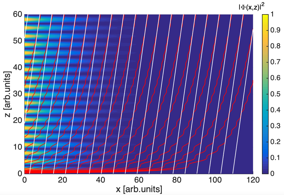
To illustrate such an effective Bohmian dynamics, Figure 1 shows typical trajectories in a microcavity. In the case of a plane wave with $\Psi \left(x\right)=e^{i{k}_{x}x}$ (see Equation (A7)), we compare the current lines obtained in the $x-z$ plane from formula $\mathbf{v}=\mathcal{S}/u$ (red curves) and the averaged Formula (39) (white line). In both cases, the vertical movement corresponds to radiative leaks. Furthermore, planar motion is associated with an energy flow along the x axis. For the present case (purely theoretical), we have imposed ${\epsilon }^{\prime }=1$, ${\epsilon }^{″}=0$, $m=1$ (arbitrary units), $D_0=23\lambda =46\pi /m$, $E/m={10}^{-4}$, $V=0$, and $\Gamma /m={10}^{-3}$. The intensity plot ${|\Phi (x,z)|}^2$ (with $\Phi (x,z)=\Psi \left(x\right)sin\chi$) shows the decaying of the wave along the $+x$ direction and the (weak) growing intensity along the $+z$ direction.

Summarizing the results obtained in this Section 4.1, we have clearly derived effective 2D Bohmian mechanics describing the motion of the energy fluid defined by Maxwell’s equations in the presence of radiative losses in the third direction, $+z$. The key point is that although the Maxwell theory used here is purely deterministic and without intrinsic dissipation (i.e., without Ohmic loss), the effective Schrödinger equation implies a complex potential $V-i{\displaystyle \frac{\Gamma }{2}}$ whose imaginary part is related to radiative leakage, i.e., to the weak propagation of waves in the $+z$ direction toward the exit of the planar cavity. In quantum mechanics, a complex potential is used to model a non-elastic interaction or dissipation due to coupling with an environment. We have therefore constructed a theory that, from a 2D perspective, appears to be dissipative. The Bohmian trajectories involved in this 2D dynamics must therefore in some way involve a stochastic element linked to this effective dissipation, which causes trajectories to disappear due to movement in the $+z$ direction (this is of course visible in Figure 1). This point is discussed in more detail in Section 4.4 in relation to the notion of probability and ‘Bell jumps’ [11,12,13,14].

4.2. Tunnel Effect, Leakage Radiation and the Work of Sharoglazova et al. [15]

In connection with the article by Sharoglazova et al. [15], we demonstrated in [21] that for a waveguide located in the planar cavity and aligned in the $+x$ direction, the presence of a tunnel barrier implies, in the absence of radiative loss $\Gamma$ and for ${\epsilon }^{″}=0$, an imaginary wave vector $k_x^{\left(0\right)}=i\sqrt{2m\epsilon (V-E)}=i{\kappa }_x^{\left(0\right)}$ with $V-E>0$, which corresponds to a pure evanescent wave $\Psi \left(x\right)=e^{i{k}_x^{\left(0\right)}x}=e^{-{\kappa }_x^{\left(0\right)}x}$. According to our model developed in Section 3, in the absence of loss, the Bohmian velocity $v_x^{\left(0\right)}={\displaystyle \frac{1}{\epsilon m}}\mathrm{Im}\left[{\displaystyle \frac{{\partial }_x{\Psi }^{\left(0\right)}\left(x\right)}{{\Psi }^{\left(0\right)}\left(x\right)}}\right]$ is zero, and therefore, in agreement with [15], photons cannot propagate in the guide.

In contrast, when $\Gamma >0$, we have a potential $V\to V-i{\displaystyle \frac{\Gamma }{2}}$, and the wave vector becomes $k_x\simeq k_x^{\left(0\right)}+i{\displaystyle \frac{m\epsilon \Gamma }{2k_x^{\left(0\right)}}}$, which gives a non-zero dBB velocity $v_x\simeq {\displaystyle \frac{\Gamma }{2{\kappa }_x^{\left(0\right)}}}$. This corresponds to the photon flux required to resolve the paradox surrounding [15], as we have shown in more detail in [21] (i.e., for the exact configuration involving two waveguides and photon movement in the $x-y$ plane from one guide to the other by tunneling). In this article, where we do not analyze in detail the configuration presented in [15], and in order to make our response in [21] self-sufficient, we will instead illustrate the simplified case of a potential barrier located at $x=0$ with $V\left(x\right)=0$ for $x<0$ and constant $V\left(x\right)=V$ for $x>0$. This is also the configuration discussed in the recent article by Klaers et al. [37]. In the absence of loss ($\Gamma =0$, ${\epsilon }^{″}=0$), the incident field ${\Psi }^{(in,0)}\left(x\right)=e^{i{k}^{{(in,0)}_x}x}$ comes from $x<0$, with a real incident wave vector $k_x^{(in,0)}=\sqrt{2m\epsilon E}$. The total field ${\Psi }^{\left(0\right)}\left(x\right)$ is given by

$$\begin{array}{cc}\hfill {\Psi }^{\left(0\right)}\left(x\right)=e^{i{k}_x^{(in,0)}x}+R^{\left(0\right)}{e}^{-i{k}_x^{(in,0)}x}& \mathrm{for}x\le 0\\ \hfill {\Psi }^{\left(0\right)}\left(x\right)=T^{\left(0\right)}{e}^{i{k}_x^{\left(0\right)}x}& \mathrm{for}x\ge 0\end{array}$$

(40)

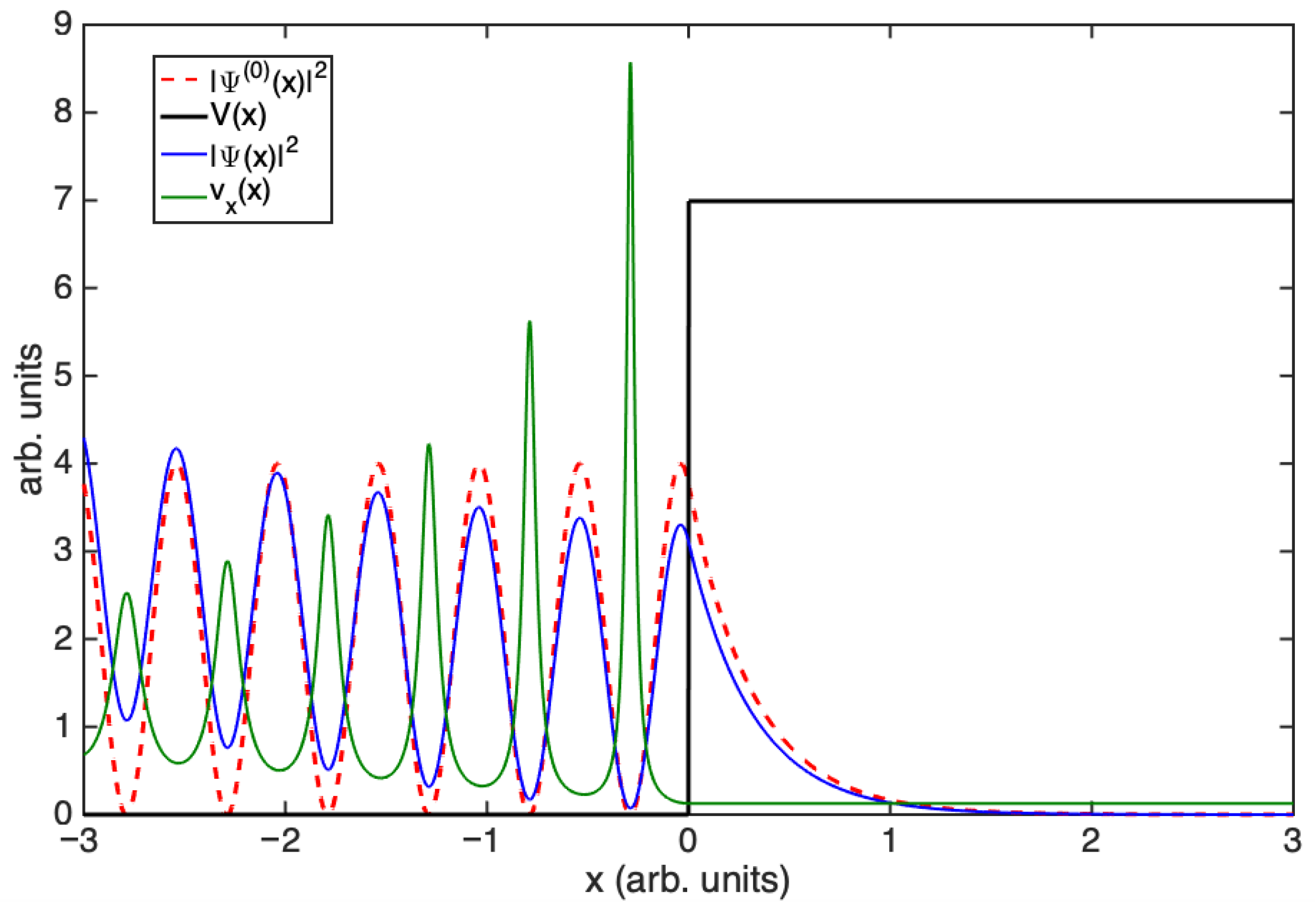
with Fresnel coefficients for reflection $R^{\left(0\right)}={\displaystyle \frac{k_x^{(in,0)}-k_x^{\left(0\right)}}{k_x^{(in,0)}+k_x^{\left(0\right)}}}$ and transmission $T^{\left(0\right)}={\displaystyle \frac{2k_x^{(in,0)}}{k_x^{\left(in\right)}+k_x^{\left(0\right)}}}$ where $k_x^{\left(0\right)}=i\sqrt{2m\epsilon (V-E)}=i{\kappa }_x^{\left(0\right)}$ as before. As illustrated in Figure 2, this corresponds to a tunnel barrier ($V>E$) with a stationary field for $x<0$ and an evanescent wave for $x>0$. In this regime, the Bohmian velocity is strictly zero $v_x^{\left(0\right)}={\displaystyle \frac{1}{\epsilon m}}\mathrm{Im}\left[{\displaystyle \frac{{\partial }_x{\Psi }^{\left(0\right)}\left(x\right)}{{\Psi }^{\left(0\right)}\left(x\right)}}\right]=0$ for all x.

In the presence of radiative loss $\Gamma >0$, the potential is transformed into $V\left(x\right)\to V\left(x\right)-i{\displaystyle \frac{\Gamma }{2}}$, and the wave vectors are also modified accordingly:

$$\begin{array}{c}\hfill k_x^{(0,in)}\to k_x^{in}\simeq k_x^{(0,in)}+i{\displaystyle \frac{m\epsilon \Gamma }{2k_x^{(0,in)}}}\\ \hfill k_x^{\left(0\right)}\to k_x\simeq k_x^{\left(0\right)}+i{\displaystyle \frac{m\epsilon \Gamma }{2k_x^{\left(0\right)}}}\end{array}$$

(41)

which amounts to assigning an additional imaginary part to the wave vector for $x<0$ and an additional real part for x > 0. The total field takes the same form as Equation (40) with the transformation ${\Psi }^{\left(0\right)}\left(x\right)\to \Psi \left(x\right)$ involving the modified Fresnel coefficients $R^{\left(0\right)}\to R$ and $T^{\left(0\right)}\to R$ related to Equation (41). As illustrated in Figure 2, the new field is no longer perfectly stationary for $x<0$ nor evanescent for $x>0$. In particular, the Bohmian velocity is no longer zero along the x-axis. It is positive but not constant for $x<0$ (which corresponds to non-uniform motion in the $+x$ direction), and it is positive and constant in the region x > 0 with $v_x\simeq {\displaystyle \frac{\Gamma }{2{\kappa }_x^{\left(0\right)}}}$ as before (see Figure 2). This shows once again that the presence of radiative loss $\Gamma$ in the $+z$ direction induces motion in the x direction.

An important point that has not been discussed concerns the notion of ‘dwell time’ [38]. For the potential step considered here and in [15] this time is defined by

$$\begin{array}{c}\hfill {\tau }_{\mathrm{dwell}}={\displaystyle \frac{{\int }_0^{+\infty }dx{|\Psi \left(x\right)|}^2}{J^{\left(in\right)}}}\end{array}$$

(42)

where $J^{\left(in\right)}$ is the incident probability current on the potential step. In the present case, in the absence of radiative loss (i.e., $\Gamma =0$), we have $J^{(0,in)}=v^{(0,in)}={\displaystyle \frac{k_x^{(0,in)}}{\epsilon m}}=\sqrt{{\displaystyle \frac{2E}{m\epsilon }}}$, and therefore,

$$\begin{array}{c}\hfill {\tau }_{\mathrm{dwell}}={\displaystyle \frac{|T^{\left(0\right)}{|}^2{\int }_0^{+\infty }dx{e}^{-2{\kappa }_x^{\left(0\right)}x}}{v^{(0,in)}}}={\displaystyle \frac{|T^{\left(0\right)}{|}^2}{2{\kappa }_x^{\left(0\right)}{v}^{(0,in)}}}\end{array}$$

(43)

which is the formula obtained in [15,37]. However, in [15,37], it is claimed that the de Broglie–Bohm theory implies a zero incident velocity for $x<0$ and therefore that ${\tau }_{\mathrm{dwell}}$ would be infinite. As they wrote [15],

‘Thus, the dwell time for scattering at a semi-infinite step potential is an example of a physical quantity that, although identically defined and measurable in both Bohmian mechanics and standard quantum mechanics, yields different values in the two theories.’

However we disagree with this conclusion.

Firstly, what is actually infinite (in absence of loss $\Gamma$) is a different dwell time defined by

$$\begin{array}{c}\hfill {\tau }_{\mathrm{dwell}}^{\prime }={\displaystyle \frac{{\int }_0^{+\infty }dx{|\Psi \left(x\right)|}^2}{J_{\Psi }\left(0\right)}}\end{array}$$

(44)

where $J_{\Psi }\left(x\right)={\displaystyle \frac{1}{\epsilon m}}\mathrm{Im}\left[{{\Psi }^{\left(0\right)}\left(x\right)}^{*}{\partial }_x{\Psi }^{\left(0\right)}\left(x\right)\right]=0$ is the actual vanishing current. The two dwell times certainly do not have the same physical interpretation and should not be confused with each other.

Secondly, we must actually consider the physical situation with $\Gamma >0$. If we do this, the first dwell time ${\tau }_{\mathrm{dwell}}$ is slightly modified. Indeed, in presence of radiative damping $\Gamma >0$, we have $J^{in}=v^{in}=\mathrm{Im}\left[{\displaystyle \frac{k_x^{\left(in\right)}}{\epsilon m}}\right]\simeq v^{0,in}$ (see Equation (41)), and we have instead

$$\begin{array}{c}\hfill {\tau }^{\mathrm{dwell}}\simeq {\displaystyle \frac{{\left|T\right|}^2}{2{\kappa }_x^{\left(0\right)}{v}_{in}}}\end{array}$$

(45)

with ${\left|T\right|}^2\simeq {\left|T^{\left(0\right)}\right|}^2[1+{\displaystyle \frac{m^2{\epsilon }^2{\Gamma }^2}{4}}{({\displaystyle \frac{1}{{\left(k_x^{(0,in)}\right)}^2}}-{\displaystyle \frac{1}{k_x^{(0,in)}{\kappa }_x^{\left(0\right)}}})}^2]$. As a first approximation, the lossless result Equation (43) is therefore unchanged. The second dwell time ${\tau }_{\mathrm{dwell}}^{\prime }$ is, however, very different. Indeed, we obtain

$$\begin{array}{c}\hfill {\tau }_{\mathrm{dwell}}^{\prime }={\displaystyle \frac{{\left|T\right|}^2{\int }_0^{+\infty }dx{e}^{-2{\kappa }_x^{\left(0\right)}x}}{{\left|T\right|}^2\frac{\Gamma }{2{\kappa }_x^{\left(0\right)}}}}={\displaystyle \frac{1}{\Gamma }}\end{array}$$

(46)

This time ${\tau }_{\mathrm{dwell}}^{\prime }$ has a direct interpretation as the typical particle accumulation time in the region $x>0$. The fact that ${\tau }_{\mathrm{dwell}}^{\prime }$ is directly equal to the characteristic damping time ${\Gamma }^{-1}$ is physically significant.

Note, however, that neither ${\tau }_{\mathrm{dwell}}$ nor ${\tau }_{\mathrm{dwell}}^{\prime }$ require Bohmian theory: the results are a pure consequence of quantum mechanics and are independent of interpretation. If we nevertheless seek to define a typically Bohmian time, we can consider the time taken to travel between the potential jump $x=0$ and any point $x>0$ [39]. If we include dissipation $\Gamma$, we obtain

$$\begin{array}{c}\hfill {\tau }_{\mathrm{dBB}}\left(x\right)={\int }_0^{+\infty }{\displaystyle \frac{dx}{v_x\left(x\right)}}={\int }_0^{+\infty }dx{\displaystyle \frac{{|\Psi \left(x\right)|}^2}{J_{\Psi }\left(x\right)}}\simeq {\displaystyle \frac{2k_x^{(0,in)}x}{\Gamma }}\end{array}$$

(47)

As we can see, this time, which increases linearly, is physically connected to ${\tau }_{\mathrm{dwell}}^{\prime }$ (it diverges if $\Gamma =0$). In particular, for a distance traveled $x={\displaystyle \frac{1}{2k_x^{(0,in)}}}$ (i.e., the propagation length), the two times are equal, which is physically intuitive.

In any case, this shows that the de Broglie–Bohm theory is unaffected by the results of the experiments and analyses carried out in [15]. The theory is even reinforced by its effectiveness in describing propagation processes in a real situation involving a potential jump and radiative dissipation $\Gamma$.

4.3. Generalization for Particles with Spin-$1/2$

The analysis in the previous sections was limited to the case of a linear polarization field $\mathcal{E}=\widehat{\mathbf{e}}\Phi (x,y,z)e^{-i\omega t}$ corresponding to the case considered in [15,16,21]. However, it is possible to extend the result a little further to more complex fields written as

$$\begin{array}{c}\hfill \mathcal{E}=[\widehat{\mathbf{x}}{\Phi }_x(x,y,z)+\widehat{\mathbf{y}}{\Phi }_y(x,y,z)]e^{-i\omega t}=[{\widehat{\mathbf{e}}}_{+}{\Phi }_{+}(x,y,z)+{\widehat{\mathbf{e}}}_{-}{\Phi }_{-}(x,y,z)]e^{-i\omega t},\end{array}$$

(48)

where ${\widehat{\mathbf{e}}}_{\pm }={\displaystyle \frac{\widehat{\mathbf{x}}\pm i\widehat{\mathbf{y}}}{\sqrt{2}}}$ denotes left- or right-handed circular polarization unit vectors and where we have ${\Phi }_{\pm }(x,y,z)={\Psi }_{\pm }(x,y)f_{x,y}\left(z\right)$, ${\Phi }_x(x,y,z)={\Psi }_x(x,y)f_{x,y}\left(z\right)$, ${\Phi }_x(x,y,z)={\Psi }_y(x,y)f_{x,y}\left(z\right)$ with $f_{xy}\left(z\right)$ given by Equation (36) and ${\Psi }_{\pm }(x,y)={\displaystyle \frac{{\Psi }_x(x,y)\mp i{\Psi }_y(x,y)}{\sqrt{2}}}$ two-wave functions forming a Pauli spinor:

$$\begin{array}{c}\hfill \mathfrak{F}(x,y)=\left(\begin{array}{c}{\Psi }_{+}(x,y)\\ {\Psi }_{-}(x,y)\end{array}\right)\end{array}$$

(49)

To do this, we use a decomposition obtained by M. Berry [40] for the Poynting vector, which is written as

$$\begin{array}{c}\hfill \mathcal{S}\simeq {\displaystyle \frac{2}{m}}\mathrm{Im}[{\mathcal{E}}^{*}\times (\mathbf{\nabla }\times \mathcal{E})]={\displaystyle \frac{2}{m}}\mathrm{Im}\left[{\mathcal{E}}^{*}(\mathbf{\nabla })\mathcal{E}\right]+{\displaystyle \frac{1}{m}}\mathbf{\nabla }\times \mathrm{Im}[{\mathcal{E}}^{*}\times \mathcal{E}]\end{array}$$

(50)

with $\mathit{A}(\mathbf{\nabla })\mathit{B}={\sum }_{k=1}^{k=3}{A}_k\mathbf{\nabla }{B}_k$. This formula contains two contributions, one ${\mathcal{S}}_{orb}={\displaystyle \frac{2}{m}}\mathrm{Im}\left[{\mathcal{E}}^{*}(\mathbf{\nabla })\mathcal{E}\right]$ associated with orbital motion and the other ${\mathcal{S}}_{spin}={\displaystyle \frac{1}{m}}\mathbf{\nabla }\times \mathrm{Im}[{\mathcal{E}}^{*}\times \mathcal{E}]$ associated with spinorial motion. We deduce the velocity of the energy fluid:

$$\begin{array}{c}\hfill \mathbf{v}={\mathbf{v}}_{orb}+{\mathbf{v}}_{spin}={\displaystyle \frac{{\mathcal{S}}_{orb}}{\mathcal{U}}}+{\displaystyle \frac{{\mathcal{S}}_{spin}}{\mathcal{U}}}\end{array}$$

(51)

with $\mathcal{U}\simeq {\epsilon }^{\prime }{\left|\mathcal{E}\right|}^2+{\displaystyle \frac{1}{m^2}}{|\mathbf{\nabla }\times \mathcal{E}|}^2$. Using the Pauli spinor $\mathfrak{F}(x,y)$ we obtain the following, as for Equations (38) and (39):

$$\begin{array}{c}\hfill \langle {\mathbf{v}}_{orb}\rangle ={\displaystyle \frac{{\int }_0^{D_0}dz{\mathcal{S}}_{orb}}{{\int }_0^{D_0}dz\mathcal{U}}}={\displaystyle \frac{1}{m{\epsilon }^{\prime }}}{\displaystyle \frac{\mathrm{Im}\left[{\mathfrak{F}}^{†}{\mathbf{\nabla }}_{\left|\right|}\mathfrak{F}\right]}{{\mathfrak{F}}^{†}\mathfrak{F}}}+{\displaystyle \frac{\Gamma D_0}{2}}\widehat{\mathbf{z}}\end{array}$$

(52)

For the spinorial term, we find, at the leading order,

$$\begin{array}{c}\hfill {\mathcal{S}}_{spin}\simeq {\displaystyle \frac{{sin}^2{\chi }_0}{m}}{\mathbf{\nabla }}_{\left|\right|}\times \left({\mathfrak{F}}^{†}{\sigma }_z\mathfrak{F}\widehat{\mathbf{z}}\right)\end{array}$$

(53)

which implies an average velocity of

$$\begin{array}{c}\hfill \langle {\mathbf{v}}_{spin}\rangle ={\displaystyle \frac{{\int }_0^{D_0}dz{\mathcal{S}}_{spin}}{{\int }_0^{D_0}dz\mathcal{U}}}={\displaystyle \frac{1}{2m{\epsilon }^{\prime }}}{\displaystyle \frac{{\mathbf{\nabla }}_{\left|\right|}\times \left({\mathfrak{F}}^{†}{\sigma }_z\mathfrak{F}\widehat{\mathbf{z}}\right)}{{\mathfrak{F}}^{†}\mathfrak{F}}}\end{array}$$

(54)

where ${\sigma }_z=\left(\begin{array}{cc}1& 0\\ 0& -1\end{array}\right)$ is the Pauli matrix for the z direction.

It is remarkable to note that the planar part of this velocity field, i.e., $\langle {\mathbf{v}}_{orb,\left|\right|}\rangle +\langle {\mathbf{v}}_{spin}\rangle ={\displaystyle \frac{1}{m{\epsilon }^{\prime }}}{\displaystyle \frac{\mathrm{Im}\left[{\mathfrak{F}}^{†}{\mathbf{\nabla }}_{\left|\right|}\mathfrak{F}\right]}{{\mathfrak{F}}^{†}\mathfrak{F}}}+{\displaystyle \frac{1}{2m{\epsilon }^{\prime }}}{\displaystyle \frac{{\mathbf{\nabla }}_{\left|\right|}\times \left({\mathfrak{F}}^{†}{\sigma }_z\mathfrak{F}\widehat{\mathbf{z}}\right)}{{\mathfrak{F}}^{†}\mathfrak{F}}}$, can be deduced from the Bohmian interpretation of Pauli’s equation:

$$\begin{array}{c}\hfill i{\partial }_t\mathfrak{F}(x,y,t)=-{\displaystyle \frac{{\mathbf{\nabla }}_{\left|\right|}^2}{2{\epsilon }^{\prime }m}}\mathfrak{F}(x,y,t)+(V(x,y)-i{\displaystyle \frac{\Gamma }{2}}-im{\displaystyle \frac{{\epsilon }^{″}}{2{\epsilon }^{\prime }}})\mathfrak{F}(x,y,t)\end{array}$$

(55)

for the spinor $\mathfrak{F}(x,y,t)$. Indeed, for Equation (55) the conservation law for the probability fluid with density ${\mathfrak{F}}^{†}\mathfrak{F}$ (see the next subsection for an interpretation of the conservation law) leads to the probability current

$$\begin{array}{c}\hfill {\mathbf{J}}_{\left|\right|}(x,y,t)={\displaystyle \frac{\mathrm{Im}\left[{\mathfrak{F}}^{†}{\mathbf{\nabla }}_{\left|\right|}\mathfrak{F}\right]}{m{\epsilon }^{\prime }}}+{\displaystyle \frac{{\mathbf{\nabla }}_{\left|\right|}\times \left({\mathfrak{F}}^{†}{\sigma }_z\mathfrak{F}\widehat{\mathbf{z}}\right)}{2m{\epsilon }^{\prime }}}\end{array}$$

(56)

which contains convective and spinorial contributions. This decomposition is well known in particle physics [41] and can be deduced from the Dirac Equation (Gordon decomposition), which plays an important role in Bohmian mechanics in justifying the correct form of the probability current for a spin-$1/2$ particle [42,43,44]. It implies the de Broglie–Bohm velocity:

$$\begin{array}{c}\hfill {\mathbf{v}}_{dBB,\left|\right|}(x,y,t)={\displaystyle \frac{\mathrm{Im}\left[{\mathfrak{F}}^{†}{\mathbf{\nabla }}_{\left|\right|}\mathfrak{F}\right]}{m{\epsilon }^{\prime }{\mathfrak{F}}^{†}\mathfrak{F}}}+{\displaystyle \frac{{\mathbf{\nabla }}_{\left|\right|}\times \left({\mathfrak{F}}^{†}{\sigma }_z\mathfrak{F}\widehat{\mathbf{z}}\right)}{2m{\epsilon }^{\prime }{\mathfrak{F}}^{†}\mathfrak{F}}}\\ \hfill ={\displaystyle \frac{\mathrm{Im}[{\Psi }_x^{†}{\mathbf{\nabla }}_{\left|\right|}{\Psi }_x+{\Psi }_y^{†}{\mathbf{\nabla }}_{\left|\right|}{\Psi }_y]}{m{\epsilon }^{\prime }\left(\right|{\Psi }_x{|}^2+|{\Psi }_y{|}^2)}}+{\displaystyle \frac{{\mathbf{\nabla }}_{\left|\right|}\times \left(\mathrm{Im}\left[{\Psi }_x^{*}{\Psi }_y\right]\widehat{\mathbf{z}}\right)}{m{\epsilon }^{\prime }\left(\right|{\Psi }_x{|}^2+|{\Psi }_y{|}^2)}}\\ \hfill ={\displaystyle \frac{\mathrm{Im}[{\Psi }_{+}^{†}{\mathbf{\nabla }}_{\left|\right|}{\Psi }_{+}+{\Psi }_{-}^{†}{\mathbf{\nabla }}_{\left|\right|}{\Psi }_{-}]}{m{\epsilon }^{\prime }\left(\right|{\Psi }_{+}{|}^2+|{\Psi }_{-}{|}^2)}}+{\displaystyle \frac{{\mathbf{\nabla }}_{\left|\right|}\times \left(\right[|{\Psi }_{+}{|}^2-|{\Psi }_{-}{|}^2\left]\widehat{\mathbf{z}}\right)}{2m{\epsilon }^{\prime }\left(\right|{\Psi }_{+}{|}^2+|{\Psi }_{-}{|}^2)}}\end{array}$$

(57)

which is identical to $\langle {\mathbf{v}}_{orb,\left|\right|}\rangle +\langle {\mathbf{v}}_{spin}\rangle$ deduced from energy conservation. What seems paradoxical, of course, is that the photon (a spin-1 particle by nature) in the paraxial regime behaves here like a massive spin-1/2 particle. However, we suggest that this is not so surprising if we remember that in this paraxial domain, the polarization fields of light (orthogonal to the direction of propagation z) are formally described by SU(2) (for discussions see [27,45]).

A few remarks concerning this spinorial formalism are useful here: First, note that in Bohmian theory we can define a local spin vector associated with the motion of the particle [3,4]. This is written as

$$\begin{array}{c}\hfill \Sigma (x,y,t)={\displaystyle \frac{1}{2}}{\displaystyle \frac{{\mathfrak{F}}^{†}{\sigma }_z\mathfrak{F}}{{\mathfrak{F}}^{†}\mathfrak{F}}}\widehat{\mathbf{z}}={\displaystyle \frac{1}{2}}{\displaystyle \frac{|{\Psi }_{+}{|}^2-{\left|{\Psi }_{-}\right|}^2}{|{\Psi }_{+}{|}^2+{\left|{\Psi }_{-}\right|}^2}}\widehat{\mathbf{z}}={\displaystyle \frac{\mathrm{Im}\left[{\Psi }_x^{*}{\Psi }_y\right]}{|{\Psi }_x{|}^2+{\left|{\Psi }_y\right|}^2}}\widehat{\mathbf{z}}={\Sigma }_z(x,y,t)\widehat{\mathbf{z}}\end{array}$$

(58)

because here the spin has only one component ${\Sigma }_z(x,y,t)$. In the same context, it should be observed that the role of Berry decomposition [40] in Bohmian mechanics for photons (but unrelated to the spinorial formalism used here) had already been considered [27] in connection with weak-measurement experiments by Kocsis et al. [28] to measure the Bohmian velocity field of a single photon in a paraxial regime in free space. This important point deserves further scrutiny. We point out, in relation to [27], that the spin vector $\Sigma$ is connected to the Stokes parameters $s_1,s_2,s_3$, forming a vector $\mathbf{s}$ representing the local polarization state of light on the Poincaré–Bloch sphere ($\left|\mathbf{s}\right|=1$). Thus, we have $2{\Sigma }_z=s_3$.

However, the most important observation concerns the transverse nature of the light polarization field. In fact, we did not yet take into account in our analysis (following the phenomenological model of Klaers et al. [15,16]) the transversality condition $\mathbf{\nabla }·\mathcal{E}=0$ imposed by Maxwell’s equations (condition $\mathbf{\nabla }·\mathcal{B}=0$ is directly imposed by the definition $\mathbf{\nabla }\times \mathcal{E}\simeq im\mathcal{B}$). Indeed, the constraint $\mathbf{\nabla }·\mathcal{E}=0$ reads

$$\begin{array}{c}\hfill {\partial }_x{\Psi }_x+{\partial }_y{\Psi }_y=-{\Psi }_x{\displaystyle \frac{{\partial }_x{f}_{x,y}}{f_{x,y}}}-{\Psi }_y{\displaystyle \frac{{\partial }_y{f}_{x,y}}{f_{x,y}}}=-\sqrt{{\epsilon }^{\prime }}\mathrm{cotan}\chi ({\Psi }_x{\partial }_{x}V+{\Psi }_y{\partial }_{y}V).\end{array}$$

(59)

We assume here that we work in the regime where the right-hand side is small (i.e., we neglect $\partial V$) and we write

$$\begin{array}{c}\hfill {\partial }_x{\Psi }_x+{\partial }_y{\Psi }_y={\partial }_{+}{\Psi }_{-}+{\partial }_{-}{\Psi }_{+}\simeq 0\end{array}$$

(60)

with ${\partial }_{\pm }={\displaystyle \frac{{\partial }_x\mp i{\partial }_y}{\sqrt{2}}}={\displaystyle \frac{\partial }{\partial x_{\mp }}}$ and $x_{\pm }={\displaystyle \frac{x\mp iy}{\sqrt{2}}}$. The Pauli Equation (55) and constraint (60) must therefore be solved consistently, which for a general problem does not admit any trivial solutions a priori. However, we can approximately solve the problem by introducing a stream function $Q(x,y,t)$, such that we have

$$\begin{array}{cc}\hfill {\Psi }_x=-{\partial }_{y}Q,& {\Psi }_y={\partial }_{x}Q\\ \hfill {\Psi }_{+}=-i{\partial }_{+}Q,& {\Psi }_{-}=i{\partial }_{-}Q\end{array}$$

(61)

which automatically satisfies Equation (60). In order to satisfy Pauli’s Equation (55), we impose Schrödinger’s equation for Q:

$$\begin{array}{c}\hfill i{\partial }_{t}Q(x,y,t)=-{\displaystyle \frac{{\mathbf{\nabla }}_{\left|\right|}^2}{2{\epsilon }^{\prime }m}}Q(x,y,t)+(V(x,y)-i{\displaystyle \frac{\Gamma }{2}}-im{\displaystyle \frac{{\epsilon }^{″}}{2{\epsilon }^{\prime }}})Q(x,y,t)\end{array}$$

(62)

This condition allows us to satisfy Equation (55) with the same degree of precision as for Equation (60) (i.e., by neglecting $\partial V$).

With this description, the Bohmian velocity in Equation (57) is written as

$$\begin{array}{c}\hfill {\mathbf{v}}_{dBB,\left|\right|}(x,y,t)={\displaystyle \frac{\mathrm{Im}[{\partial }_x{Q}^{†}{\mathbf{\nabla }}_{\left|\right|}{\partial }_{x}Q+{\partial }_y{Q}^{†}{\mathbf{\nabla }}_{\left|\right|}{\partial }_{y}Q]}{m{\epsilon }^{\prime }\left(\right|{\partial }_x{Q|}^2+|{\partial }_{y}Q{|}^2)}}+{\displaystyle \frac{{\mathbf{\nabla }}_{\left|\right|}\times \left(\mathrm{Im}\left[{\partial }_x{Q}^{*}{\partial }_{y}Q\right]\widehat{\mathbf{z}}\right)}{m{\epsilon }^{\prime }\left(\right|{\partial }_x{Q|}^2+|{\partial }_{y}Q{|}^2)}}\\ \hfill ={\displaystyle \frac{\mathrm{Im}[{\partial }_{+}{Q}^{†}{\mathbf{\nabla }}_{\left|\right|}{\partial }_{+}Q+{\partial }_{-}{Q}^{†}{\mathbf{\nabla }}_{\left|\right|}{\partial }_{-}Q]}{m{\epsilon }^{\prime }\left(\right|{\partial }_{+}{Q|}^2+|{\partial }_{-}Q{|}^2)}}+{\displaystyle \frac{{\mathbf{\nabla }}_{\left|\right|}\times \left(\right[|{\partial }_{+}{Q|}^2-|{\partial }_{-}{Q|}^2\left]\widehat{\mathbf{z}}\right)}{2m{\epsilon }^{\prime }\left(\right|{\partial }_{+}{Q|}^2+|{\partial }_{-}Q{|}^2)}}\end{array}$$

(63)

Strictly speaking, this dynamic must play a role in the analysis of the experiment detailed in [15] in order to go beyond the phenomenological approach based on a single wave $\Psi$ [16] and neglecting the role of polarization. A more detailed and precise analysis of the experiments reported [15] will be published at a later date. However, it should be noted that this does not alter the general conclusions of our critique presented in [21]. In particular, without going into detail, the Bohmian velocity $v_x$ along the waveguides studied in [15] (i.e., in the evanescent regime) is still quantitatively dominated by $v_x\simeq {\displaystyle \frac{\Gamma }{2\sqrt{(-2m\Delta )}}}\simeq$ 30 km/s (where $\Delta \simeq -0.04$ meV is an energy detuning [15]) in agreement with our previous analysis [21].

4.4. Conservation of Probability and Stochastic Bohmian Mechanics

It is crucial to note that the effective Schrodinger Equation (34) is non-unitary due to the presence of the complex potential $V-i{\displaystyle \frac{\Gamma }{2}}-im{\displaystyle \frac{{\epsilon }^{″}}{2{\epsilon }^{\prime }}}$. In particular, the local conservation law for the electron fluid becomes

$$\begin{array}{c}\hfill {\partial }_t{|\Psi |}^2+{\mathbf{\nabla }}_{\left|\right|}{\left(\right|\Psi |}^2{\mathbf{v}}_{dBB,\left|\right|})+(\Gamma +m{\displaystyle \frac{{\epsilon }^{″}}{{\epsilon }^{\prime }}}){|\Psi |}^2=0\end{array}$$

(64)

This equation can be derived directly from Equation (34) or from the local energy conservation condition (13) by averaging over z: ${\partial }_t{\int }_0^{D_0}dz\mathcal{U}=-{\int }_0^{D_0}dz\mathbf{\nabla }·\mathcal{S}-{\int }_0^{D_0}dz\mathcal{W}$. A similar equation is deduced from Equation (55) with the density ${\mathfrak{F}}^{†}\mathfrak{F}$ replacing ${|\Psi |}^2$ and with the spin-dependent velocity fields in Equation (57). We stress that Equation (64) involves a radiative loss term ${\Gamma |\Psi |}^2$ that must be interpreted as an effective absorption. It is indeed effective in the sense that it exists only from a perspective where we neglect the presence of the third dimension z characterized by a complex wave vector $k_z=\sqrt{{\epsilon }^{\prime }}(m+V(x,y)-i{\displaystyle \frac{\Gamma }{2}})$ appearing in Equation (36). The second loss term $m{\displaystyle \frac{{\epsilon }^{″}}{{\epsilon }^{\prime }}}{|\Psi |}^2$ is associated with internal absorption due to Ohmic dissipation. Clearly, if we are only considering the 2D motion, the two channels associated with radiative and Ohmic losses are indistinguishable. This is reminiscent of works done in quantum optics, modeling dissipation ${\epsilon }^{″}$ as effective optical channels associated with leakage [46,47].

From a Bohmian perspective, there is a strong analogy between the present model and the work of Bell and Dürr et al. in QFT based on a stochastic version of de Broglie–Bohm theory [11,12,13,14] (see also [48] for a link to measurement theory and the notion of arrival time [49,50] in Bohmian mechanics). To be more explicit would require a detailed analysis, which we will briefly outline in the following section.

First, the conservation Equation (64) characterizes a master equation for an electromagnetic fluid. The quantity $u_{2D}={\epsilon }^{\prime }{D}_0{|\Psi |}^2$ defines a surface energy density for this fluid, and $(\Gamma +m{\displaystyle \frac{{\epsilon }^{″}}{{\epsilon }^{\prime }}})u_{2D}$ quantifies the rate of disappearance of this fluid through Ohmic absorption and radiative leakage channels. In order to obtain a better Bohmian analogy, it must be possible to talk about the probability of the photon’s presence in the 2D cavity, but this controversial notion is not universally accepted in the quantum optics community (see, e.g., [51,52,53] for interesting discussions and proposals). However, in the present case, the photon is an effective particle with mass $\omega \simeq m$, and it is a priori-justified to introduce a particle surface density ${\rho }_{2D}(x,y,t)={\mathcal{U}}_{2D}(x,y,t)/\omega \simeq {\mathcal{U}}_{2D}(x,y,t)/m$.

Furthermore, although the analysis in this work is essentially classical, it can easily be extended to the quantum domain. This allows us to make a brief digression into the regime where single-photon QED is formally equivalent to Maxwell’s equations for a classical but complex valued electromagnetic field $\mathcal{E},\mathcal{B}$ (this equivalence being demonstrated, for example, in [52]). Thus, if we are limited to a single photon, the electromagnetic field of the effective particle in the cavity can be deduced from the second-quantized formalism of QED [52], and we can set

$$\begin{array}{c}\hfill \mathcal{E}(\mathbf{x},t):=\langle 0|{\widehat{\mathbf{E}}}^{(+)}(\mathbf{x},t)|1\rangle \\ \hfill \mathcal{B}(\mathbf{x},t):=\langle 0|{\widehat{\mathbf{B}}}^{(+)}(\mathbf{x},t)|1\rangle \end{array}$$

(65)

where $|0\rangle$ and $|1\rangle$ denote a Fock state with zero or one photon, respectively, and where ${\widehat{\mathbf{E}}}^{(+)}$ and ${\widehat{\mathbf{B}}}^{(+)}$ are the positive frequency parts of the quantum electromagnetic field operators. The fields (65) appear in the transition amplitudes during photon emission and absorption phenomena and are associated in [52,54] with real electromagnetic wave functions obeying classical Maxwell’s Equation (7) in the optical environment under consideration (see also [55,56,57] for a rigorous discussion in a lossy and dispersive dielectric environment).

If we limit ourselves to a phenomenological description, the photon density ${\rho }_{2D}(x,y,t)$ is associated with the second quantized wave function $\Psi (x,y,t):=\langle 0|{\widehat{\Psi }}^{(+)}(x,y,t)|1\rangle$ with

$$\begin{array}{c}\hfill {\rho }_{2D}(x,y,t)\simeq {\displaystyle \frac{{\epsilon }^{\prime }{D}_0}{m}}{|\Psi (x,y,t)|}^2\end{array}$$

(66)

In order to normalize this wave function in a lossy cavity, we can start from a wave packet defined in the distant past with an initial energy $\omega \simeq m$, which allows us to introduce a normalized wave function $\tilde{\Psi }(x,y,t)=\sqrt{\left({\displaystyle \frac{m}{{\epsilon }^{\prime }{D}_0}}\right)}\Psi (x,y,t)$ at initial time $t_0$ (i.e., $\int dxdy|\tilde{\Psi }(x,y,t_0){|}^2=1$). The effective Schrödinger Equation (34) for this wave function $\tilde{\Psi }(x,y,t)$ therefore describes a non-unitary evolution associated with a non-Hermitian Hamiltonian $\widehat{H}=-{\displaystyle \frac{{\mathbf{\nabla }}_{\left|\right|}^2}{2{\epsilon }^{\prime }m}}+V(x,y)-i{\displaystyle \frac{\Gamma }{2}}-im{\displaystyle \frac{{\epsilon }^{″}}{2{\epsilon }^{\prime }}}$ due to absorption.

According to the formalism introduced by Bell [11,12,13,14], the law of conservation of probability fluid can be written in general terms as

$$\begin{array}{c}\hfill {\partial }_t{\left|\tilde{\Psi }(x,y,t)\right|}^2=2\mathrm{Im}\left[{\tilde{\Psi }}^{*}(x,y,t)\widehat{H}\tilde{\Psi }(x,y,t)\right]\end{array}$$

(67)

in which we can distinguish between a Hermitian contribution ${\widehat{H}}^{\left(0\right)}=-{\displaystyle \frac{{\mathbf{\nabla }}_{\left|\right|}^2}{2{\epsilon }^{\prime }m}}+V(x,y)$ giving rise to $2\mathrm{Im}\left[{\tilde{\Psi }}^{*}{\widehat{H}}^{\left(0\right)}\tilde{\Psi }\right]=-{\mathbf{\nabla }}_{\left|\right|}\left(\right|\tilde{\Psi }{|}^2{\mathbf{v}}_{dBB,\left|\right|})$ associated with the deterministic evolution, and a non-Hermitian contribution ${\widehat{H}}^{\left(L\right)}=-i{\displaystyle \frac{\Gamma }{2}}-im{\displaystyle \frac{{\epsilon }^{″}}{2{\epsilon }^{\prime }}}$ leading to $2\mathrm{Im}\left[{\tilde{\Psi }}^{*}{\widehat{H}}^{\left(L\right)}\tilde{\Psi }\right]=-(\Gamma +m{\displaystyle \frac{{\epsilon }^{″}}{{\epsilon }^{\prime }}}){\left|\tilde{\Psi }\right|}^2$ and associated with losses (we checked that similar expressions are easily obtained for the spin-dependent Pauli equation). According to Bell, if $\widehat{H}$ were purely Hermitian, we could introduce a probability of quantum jumps (or Bell jumps) using the formula

$$\begin{array}{c}\hfill {\sigma }_t(x,y|x^{\prime },y^{\prime }):={\displaystyle \frac{{\mathcal{J}}_{x,y;x^{\prime },y^{\prime },t}^{+}}{|\tilde{\Psi }(x^{\prime },y^{\prime },t){|}^2}}\end{array}$$

(68)

with ${\mathcal{J}}_{x,y;x^{\prime },y^{\prime },t}=2\mathrm{Im}\left[{\tilde{\Psi }}^{*}(x,y,t){\mathcal{H}}_{x,y;x^{\prime },y^{\prime }}\tilde{\Psi }(x^{\prime },y^{\prime },t)\right]$, ${\mathcal{H}}_{x,y;x^{\prime },y^{\prime }}:=\langle x,y|\widehat{H}|x^{\prime },y^{\prime }\rangle$ and where the plus sign indicates that this probability is taken to be zero if ${\mathcal{J}}_{x,y;x^{\prime },y^{\prime },t}$ is negative. For such a Hermitian Hamiltonian, we would have ${\mathcal{H}}_{x,y;x^{\prime },y^{\prime }}={\mathcal{H}}_{x^{\prime },y^{\prime };x,y}^{*}$, ${\mathcal{J}}_{x,y;x^{\prime },y^{\prime },t}=-{\mathcal{J}}_{x^{\prime },y^{\prime };x,y,t}$, and this would imply a master equation with both source terms and loss terms:

$$\begin{array}{c}\hfill {\partial }_t|\tilde{\Psi }{(x,y,t)|}^2=\int d{x}^{\prime }d{y}^{\prime }[{\sigma }_t(x,y|x^{\prime },y^{\prime })|\tilde{\Psi }(x^{\prime },y^{\prime },t){|}^2-{\sigma }_t(x^{\prime },y^{\prime }|x,y){|\tilde{\Psi }(x,y,t)|}^2].\end{array}$$

(69)

From such a master equation, we obviously have probability conservation ${\displaystyle \frac{d}{dt}}\int dxdy{\left|\tilde{\Psi }(x,y,t)\right|}^2=0$. However, here, with the non-Hermitian operator ${\widehat{H}}^{\left(L\right)}$, we must change the definition of Bell jumps and assume the most general form, including source terms S and loss terms L:

$$\begin{array}{cc}\hfill {\sigma }_t^{\left(S\right)}(x,y|x^{\prime },y^{\prime }):={\displaystyle \frac{{\mathcal{J}}_{x,y;x^{\prime },y^{\prime },t}}{|\tilde{\Psi }(x^{\prime },y^{\prime },t){|}^2}},& {\sigma }_t^{\left(S\right)}(x^{\prime },y^{\prime }|x,y)=0\\ \hfill \mathrm{if}{\mathcal{J}}_{x,y;x^{\prime },y^{\prime },t}\ge 0\\ \hfill {\sigma }_t^{\left(L\right)}(x^{\prime },y^{\prime }|x,y):=-{\displaystyle \frac{{\mathcal{J}}_{x,y;x^{\prime },y^{\prime },t}}{|\tilde{\Psi }{(x,y,t)|}^2}},& {\sigma }_t^{\left(L\right)}(x,y|x^{\prime },y^{\prime })=0\\ \hfill \mathrm{if}{\mathcal{J}}_{x,y;x^{\prime },y^{\prime },t}\le 0\end{array}$$

(70)

which again leads to a master equation:

$$\begin{array}{c}\hfill {\partial }_t|\tilde{\Psi }{(x,y,t)|}^2=\int d{x}^{\prime }d{y}^{\prime }[{\sigma }_t^{\left(S\right)}(x,y|x^{\prime },y^{\prime })|\tilde{\Psi }(x^{\prime },y^{\prime },t){|}^2-{\sigma }_t^{\left(L\right)}(x^{\prime },y^{\prime }|x,y)|\tilde{\Psi }(x,y,t){|}^2].\end{array}$$

(71)

Here, with the separation ${\widehat{H}}^{\left(0\right)}$ and ${\widehat{H}}^{\left(L\right)}$, we have only a loss term L and no source term S, and we get

$$\begin{array}{c}\hfill {\partial }_t|\tilde{\Psi }{(x,y,t)|}^2+{\mathbf{\nabla }}_{\left|\right|}\left(\right|\tilde{\Psi }{|}^2{\mathbf{v}}_{dBB,\left|\right|})=-\int d{x}^{\prime }d{y}^{\prime }{\sigma }^{\left(L\right)}(x^{\prime },y^{\prime }|x,y){\left|\tilde{\Psi }(x,y,t)\right|}^2.\end{array}$$

(72)

where ${\sigma }^{\left(L\right)}(x^{\prime },y^{\prime }|x,y)=(\Gamma +m{\displaystyle \frac{{\epsilon }^{″}}{{\epsilon }^{\prime }}})\delta (x-x^{\prime })\delta (y-y^{\prime })$. The presence of the Dirac distribution implies that this quantum jump process is locally defined and occurs only if $x=x^{\prime }$ and $y=y^{\prime }$. Physically, Bell’s jump corresponds here to the disappearance of a particle at point $x,y$ associated with absorption. Note that we have ${\displaystyle \frac{d}{dt}}\int dxdy|\tilde{\Psi }{(x,y,t)|}^2=-(\Gamma +m{\displaystyle \frac{{\epsilon }^{″}}{{\epsilon }^{\prime }}})\int dxdy{\left|\tilde{\Psi }(x,y,t)\right|}^2$, implying an exponential decay $\int dxdy|\tilde{\Psi }{(x,y,t)|}^2=e^{-(\Gamma +m{\displaystyle \frac{{\epsilon }^{″}}{{\epsilon }^{\prime }}})(t-t_0)}$ of the photon probability in the cavity. Such a Bell-type stochastic dynamic (based on a non-Hermitian Hamiltonian) implies that the effective 2D photon trajectories in the planar microcavity can be interrupted at a rate $(\Gamma +m{\displaystyle \frac{{\epsilon }^{″}}{{\epsilon }^{\prime }}}){\left|\tilde{\Psi }\right|}^2$ per unit time and surface area.

A few remarks on the significance of our stochastic model are useful here:

(1) First, it is not really necessary to consider the stochastic approach in order to interpret the experiments described in [15] and criticized in [21]. In fact, the Ohmic losses proportional to ${\epsilon }^{″}$ are negligible here, and only the radiative losses related to $\Gamma$ remain. The stochastic interpretation is only useful in effective 2D modeling that forgets the physical nature of radiative losses (leakage) as a photonic movement along the third dimension z and directed toward the outside of the optical cavity.

(2) This contrasts sharply with other analyses [58,59] (see also [37]), which have attempted to respond to Sharoglazova et al. [15], and which rely on an intrinsically stochastic modified Bohmian dynamics in order to describe the passage and propagation of photons between the waveguides considered in [15]. In particular, the method used in [58,59] is based on a two-fluid approach [60] already considered by Takabayasi in their pioneering work on Bohmian mechanics [61] and is related to Bell jumps [11,12,13,14]. In the present case, it remains essentially phenomenological and allows the jump from one waveguide to another (in the $\pm y$ direction) to be described stochastically. For motion in the x direction, refs. [58,59] apparently agrees with [15] and considers that the traditional Bohmian velocity—the one we use in this work—is zero (in a more recent version of [59], the author added an effect related to the temporal width of the pulse in order to obtain a non-zero Bohmian velocity along x, but as we have shown in [21], the effect is extremely weak compared to the leakage used here and in our comment [21]). What we have shown in [21] and here (see Section 4.2) is that the radiative losses $\Gamma >0$ resulting from a deterministic approach are sufficient to generate a non-zero velocity field in the $x-y$ plane, which also allows photons to be transferred in the $+x$ direction and from one optical waveguide to another in the $\pm y$ direction [21].

4.5. Summary of the Results Obtained in This Section

It is important to briefly summarize the results obtained in this Section 4. We can distinguish three regimes of increasing complexity.

(i) First, if we assume a cavity with loss but neglect the role of ohmic dissipation ${\epsilon }^{″}$ and polarization, we have constructed an effective Bohmian theory of light in the cavity capable of accounting for all the results observed in [15]. This theory is completely deterministic, and radiative leaks in the $+z$ direction play a key role in the theoretical analysis. Indeed, it is these growing waves in the $+z$ direction that allow energy and information to reach the camera located at a great distance in the $+z$ direction (i.e., far from the cavity). In return, these radiative losses are also responsible for the existence of a propagative contribution and therefore a Bohmian velocity in the microcavity plane in a (evanescent) regime where a lossless theory would predict a zero velocity. This, in conjunction with our more specific analysis in our comment [21] concerning the 2D device analysed in [15], is sufficient to completely defend the (essentially) deterministic Bohmian theory against its critics.

(ii) In a second step, we can include the polarization of light in the $x-y$ plane of the cavity. This allowed us to establish a generalization of the cavity model developed in [15,16] and demonstrate that the photon (a particle with spin-1) behaves in this effect like a massive particle with spin-1/2. The immense potential of this result becomes clear when we consider, for example, that the Bohmian trajectories for such a particle (described by the Pauli equation) are generally much more complex than for a spinless particle. This offers very interesting experimental and theoretical possibilities that will be studied in the near future.

(iii) In a third regime, we can also include losses due to ohmic dissipation proportional to the imaginary part ${\epsilon }^{″}$. This contribution implies that light energy is absorbed by matter during propagation, and therefore, unlike in case i), we can no longer rely on a purely deterministic Bohmian approach. The energy fluid conservation equation contains a sink term for the disappearance of photons. Note that this approach can be interpreted stochastically by introducing “Bell jumps” occurring randomly during propagation in the cavity. On the other hand, this absorption, viewed in an effective two-dimensional manner, is formally equivalent to the dynamics of radiative loss, since the presence of a complex potential involving $V-i\Gamma /2$ also introduces a form of dissipation. This shows that, from a 2D perspective, a Bohmian approach to the disappearance of particles by leakage or absorption has the same effect.

5. Final Remarks and Conclusions

To conclude this work, it is important to re-examine the context in which the present analysis is done. We recall that the article by Sharoglazova et al. [15] has sparked significant attention in both the scientific community [21,37,58,59] (see also [62,63,64,65,66,67]) and the media [17,18,19,20], due to its striking claim that a micro-photonics experiment challenges—or even refutes—the de Broglie–Bohm interpretation of quantum mechanics.

Their experiment uses evanescent waves confined in parallel optical waveguides, in a regime where Maxwell’s equations are formally equivalent to an effective Schrödinger equation—thus enabling a photonic analog of 2D Bohmian mechanics. Their central claim is that while Bohmian mechanics predicts zero particle velocity in evanescent waves, their observations show light “hopping” between guides, and they even propose an experimental reconstruction of a velocity field that differs from the Bohmian one (their velocity exists in evanescent fields). They argue that this reveals a fundamental contradiction with Bohmian theory, which should therefore be revised or extended.

In our response [21], we have shown that this interpretation is incorrect and that the issue stems mostly from a mischaracterization of radiative (i.e., leaky) waves (a second contribution is associated with the finite temporal witdh of the excitation but is quantitatively much smaller). The authors of [15] perceive a contradiction in ‘observing’ photon motion where Bohmian theory predicts none. They introduce a different (i.e., non Bohmian) definition of speed, which is not vanishing in a pure evanescent field. However, the real question we ask is as follows: why assume that a velocity must be assigned to photons in such a waveguide configuration, especially in the evanescent regime?

As we have shown in [21], the existence of a velocity in a evanescent field arises because the camera records a signal: light couples from the pump laser to a molecular medium and emits photons into the waveguides, and these are finally imaged. This suggests motion—hence the need for a velocity field, even in an evanescent context. Moreover, since Bohmian velocity cancels out in an ideal evanescent field, this suggests a contradiction with de Broglie–Bohm theory, which is why Sharoglazova et al. [15] believe they have refuted Bohmian theory. As a solution or alternative the authors of [15] introduce another operational definition of velocity that can be deduced from the populations of photons observed in their optical waveguides. This essentially instrumentalist approach is perfectly justified a priori, and their analysis is very interesting. It should be noted that in a recent commentary, Klaers et al. [37] defend their approach by linking it to a modified Bohmian theory involving fundamental stochasticity (however, they continue to see a difficulty in the “simple” and deterministic Bohmian theory that we defend in [21] and in this paper).

However, the most natural and general definition of velocity should be based on the energy flux passing through the waveguides in the microcavity. Indeed, the observation of photons on the camera is directly related to electromagnetic energy transported through the optical system. Moreover, and therein lies their fundamental oversight, Bohmian mechanics here is only an effective framework derived from Maxwell’s equations. A non-zero Bohmian velocity is directly linked to a non-zero Poynting vector. The present work clearly justifies this point, since Bohmian mechanics is actually an alternative hydrodynamic formulation of Maxwell’s theory in the microcavity. The very fact that we detect light associated with evanescent waves implies, through continuity, that the Bohmian velocity cannot be strictly zero inside the cavity. The wave cannot be purely evanescent: This looks like a paradox.

In ref. [21] we demonstrated through detailed analysis that the observed signals necessarily involve optical losses—in particular, leakage from the microcavity—which are essential for the imaging process itself. These losses give rise to a finite Poynting vector and hence a non-zero Bohmian velocity inside the cavity. The new analysis provided here confirms this finding and gives a firm foundation to the Bohmian analogy. This resolves the apparent paradox and fully agrees with all data [15] without altering or weakening Bohmian theory.

A technical point that we developed in Appendix A concerns the link between leaky waves, which are by definition divergent, and the finite far-field imaged by a microscope detecting radiative leaks from the cavity. We have shown (drawing on classical work [35,36,68,69,70]) that leaky waves leave their fingerprints in the optical far-field and do indeed provide a physical understanding of the propagation processes involved in optical microcavities.

Before concluding this topic, we would like to emphasize the high quality of the quantitative analysis and experience developed by Sharoglazova et al. [15,16,37]. This analysis has brought de Broglie Bohm’s theory back into the spotlight for this centenary of quantum mechanics (and also of the pilot-wave theory). Although our analysis tends to refute some of the claims made by the authors, we believe that, ultimately, our critical analysis may suggest future experiments using integrated 2D photonic optics (in particular, based on their elegant approach developed in [15]). Furthermore, as we mentioned, Klaers et al. are also interested in stochastic variants of an effective Bohmian approach [37]. Although this approach is by no means necessary, and as we have shown in [21] and here, an essentially deterministic approach is sufficient to fully explain the experiments, we believe that all this demonstrates the great interest and flexibility of Bohmian approaches, which, far from being refuted in any way, actually offer a picture of the quantum world without paradox or magic. In any case, this shows that fundamental questions in quantum mechanics will continue to inspire future experiments in optics.

To conclude, far beyond this debate surrounding the interpretation of [15], the formalism developed here offers a new and interesting perspective on Bohmian mechanics applied to light, which is worth summarizing. First, we started with an effective description of the classical Maxwell equations. The Bohmian formalism is constructed as an approximation, just like the effective Schrodinger equation deduced in the paraxial regime. The most important point is that we can connect the velocity deduced from the energy flow to the Bohmian velocity of the Schrodinger fluid. This formal construction is therefore independent of the more fundamental debates concerning Bohmian ontology applied to QED and the photon. Of course, the formalism can also be applied to a single photon, and the link between the two issues reappears, but this will not be analyzed in this work. Three important consequences of our work deserve further analysis: (i) the problem of spin associated with our description of an optical field (traditionally spin-1) by an effective spin-$1/2$ field connected to the Pauli equation arises; (ii) in addition to the simulation of quantum analog 2D massive spin-$1/2$ Bohmian particles in complex potential, it could be interesting to see if this method of averaging several pairs of real fields with random phases into a single complex field has deeper meaning and if it helps explain why complex fields appear so naturally in quantum theory (this issue is related to the recent controversy [71,72,73]); and (iii) the possibility of supplementing the deterministic description with a Bell-style stochastic approach allows a link to be made with modern QFT and attempts to describe a Bohmian theory with a variable number of particles [14]. We believe that all of these results can be taken as a source of inspiration for future research.

From a broader perspective, we believe that the hydrodynamic analogy justified here would allow us to analyze many two-dimensional optical phenomena in optical cavities using the concept of Bohmian trajectories. Of course, current works are still limited and approximate because they neglect the polarization and spin effects associated with the E and B fields. However, as we have shown, a more general effective Bohmian dynamics based on Pauli’s equation for a spin-$1/2$ particle must actually apply in a planar optical microcavity. By analogy with the Dirac equation [3,4], it should be possible to reveal contributions related to polarization in the energy current and in the Bohmian velocity (this is strongly related to recent questions concerning arrival time for electrons in Bohmian mechanics [48,49,50]). This opens up interesting prospects for this work in connection, with developments in nanophotonics involving highly polarized surface states such as topological and chiral systems.

References

1. Bacciagaluppi, G.; Valentini, A. Quantum Theory at the Crossroads: Reconsidering the 1927 Solvay Conference; Cambridge University Press: Cambridge, UK, 2009. [Google Scholar]
2. Bohm, D. A suggested interpretation of the quantum theory in terms of “hidden” variables. I. Phys. Rev. 1952, 85, 166–179. [Google Scholar] [CrossRef]
3. Bohm, D.; Hiley, B.J. The Undivided Universe; Routledge: London, UK, 1993. [Google Scholar]
4. Holland, P. The Quantum Theory of Motion; Cambridge University Press: London, UK, 1993. [Google Scholar]
5. Dürr, D.; Teufel, S. dBB Mechanics: The Physics and Mathematics of Quantum Theory; Springer: Berlin/Heidelberg, Germany, 2010. [Google Scholar]
6. Dürr, D.; Lazarovici, D. Understanding Quantum Mechanics; Springer Nature: Cham, Switerland, 2020. [Google Scholar]
7. Bohm, D. A suggested interpretation of the quantum theory in terms of “hidden” variables. II. Phys. Rev. 1952, 85, 180–193. [Google Scholar] [CrossRef]
8. Struyve, W. Pilot-wave theory and quantum fields. Rep. Prog. Phys. 2010, 73, 106001. [Google Scholar] [CrossRef] [PubMed]
9. Colin, S. Beables for quantum electrodynamics. Ann. Fond. Louis Broglie 2004, 29, 273–296. [Google Scholar]
10. Deckert, D.-A.; Esfeld, M.; Oldofredi, A. A persistent particle ontology for quantum field theory in terms of the Dirac sea. Br. J. Philos. Sci. 2019, 70, 747–770. [Google Scholar] [CrossRef]
11. Bell, J.S. Beables for quantum field theory. Phys. Rep. 1986, 137, 49–54. [Google Scholar] [CrossRef]
12. Sudbery, A. Objective interpretations of quantum mechanics and the possibility of a deterministic limit. J. Phys. A 1987, 20, 1743–1750. [Google Scholar] [CrossRef]
13. Vink, J.C. Quantum mechanics in terms of discrete beables. Phys. Rev. A 1993, 48, 1808–1818. [Google Scholar] [CrossRef]
14. Dürr, D.; Goldstein, S.; Tumulka, R.; Zanghí, N. Bohmian mechanics and quantum field theory. Phys. Rev. Lett. 2004, 93, 090402. [Google Scholar] [CrossRef]
15. Sharoglazova, V.; Puplauskis, M.; Mattschas, C.; Toebes, C.; Klaers, J. Energy–speed relationship of quantum particles challenges Bohmian mechanics. Nature 2025, 643, 67–72. [Google Scholar] [CrossRef]
16. Klaers, J.; Sharoglazova, V.; Toebes, C. Particle motion associated with wave function density gradients. Phys. Rev. A 2023, 107, 052201. [Google Scholar] [CrossRef]
17. Fedrizzi, A.; Biancalana, F. Tunnelling photons challenge interpretation of quantum mechanics. Nature 2025, 643, 37–38. [Google Scholar] [CrossRef] [PubMed]
18. Gibney, E. ‘Tour de force’ experiment probes quantum tunnelling in action. Nature 2025, ahead of print. [Google Scholar] [CrossRef] [PubMed]
19. Gibney, E. Physicists disagree wildly on what quantum mechanics says about reality, Nature survey shows. Nature 2025, 643, 1175–1179. [Google Scholar] [CrossRef]
20. Wogan, T. Bohmian mechanics challenged. Phys. World 2025, 38, 9. [Google Scholar] [CrossRef]
21. Drezet, A.; Lazarovici, D.; Nabet, B. Comment on ‘Energy-speed relationship of quantum particles challenges Bohmian mechanics’. arXiv 2025, arXiv:2508.04756. [Google Scholar]
22. Saleh, B.E.A.; Teich, M.C. Fundamentals of Photonics; John Wiley and Sons: Hoboken, NJ, USA, 2007. [Google Scholar]
23. De Broglie, L. Sur la définition générale de la correspondance entre onde et mouvement. Comptes Rendus Acad. Sci. Paris 1924, 179, 39–40. [Google Scholar]
24. De Broglie, L. Ondes et Mouvements; Gauthier-Villars: Paris, France, 1926. [Google Scholar]
25. Slater, J.C. Light quanta and wave mechanics. Phys. Rev. 1928, 31, 895–899. [Google Scholar] [CrossRef]
26. Sanz, A.S.; Davidovic, M.D.; Bozic, M. Bohmian-based approach to Gauss–Maxwell beams. Appl. Sci. 2020, 10, 1808. [Google Scholar] [CrossRef]
27. Bliokh, K.Y.; Bekshaev, A.Y.; Kofman, A.G.; Nori, F. Photon trajectories, anomalous velocities and weak measurements: A classical interpretation. New J. Phys. 2013, 15, 073022. [Google Scholar] [CrossRef]
28. Kocsis, S.; Braverman, B.; Ravets, S.; Stevens, M.J.; Mirin, R.P.; Shalm, L.K.; Steinberg, A.M. Observing the average trajectories of single photons in a two-slit interferometer. Science 2011, 332, 1170–1173. [Google Scholar] [CrossRef] [PubMed]
29. Landau, L.D.; Lifchitz, E.M. Electrodynamics of Continuous Media; Butterworth-Heinemann: Oxford, UK, 2002. [Google Scholar]
30. Jackson, J.D. Classical Electrodynamics, 3rd ed.; John Wiley and Sons: Hoboken, NJ, USA, 1999. [Google Scholar]
31. Lienert, M.; Tumulka, R. Multi-time version of the Landau-Peirls formulation of quantum electrodynamics. Ann. Phys. 2025, 479, 170043. [Google Scholar] [CrossRef]
32. Landau, L.; Peierls, R. Quantenelektrodynamik im Konfigurationsraum. Z. Phys. 1930, 62, 188–200. [Google Scholar] [CrossRef]
33. Burke, J.J.; Stegeman, G.I.; Tamir, T. Surface-polariton-like waves guided by thin lossy films. Phys. Rev. B 1986, 33, 5186–5201. [Google Scholar] [CrossRef]
34. Jackson, D.R.; Oliner, A.A. Leaky-wave antennas. In Modern Antenna Handbook; Balanis, C.A., Ed.; John Wiley and Sons: Hoboken, NJ, USA, 2007; pp. 325–367. [Google Scholar]
35. Brekhovskikh, L.M. Waves in Layered Media; Academic Press: New York, NY, USA, 1960; Chapter 4. [Google Scholar]
36. Drezet, A.; Genet, C. Imaging surface plasmons: From leaky waves to far-field radiation. Phys. Rev. Lett. 2013, 110, 213901. [Google Scholar] [CrossRef]
37. Klaers, J.; Sharoglazova, V.; Puplauskis, M. Reaffirming a challenge to Bohmian mechanics. arXiv 2025, arXiv:2509.06584. [Google Scholar] [CrossRef]
38. Büttiker, M.; Landauer, R. Traversal time for tunneling. Phys. Rev. Lett. 1982, 49, 1739–1742. [Google Scholar] [CrossRef]
39. Spiller, T.P.; Clark, T.D.; Prance, R.J.; Prance, H. Barrier traversal time in the quantum potential picture. Europhys. Lett. 1990, 12, 1–4. [Google Scholar] [CrossRef]
40. Berry, M.V. Optical currents. J. Opt. A Pure Appl. Opt. 2009, 11, 094001. [Google Scholar] [CrossRef]
41. Bjorken, J.D.; Drell, S.D. Relativistic Quantum Theory; McGraw-Hill: New York, NY, USA, 1964. [Google Scholar]
42. Holland, P. Uniqueness of paths in quantum mechanics. Phys. Rev. A 1999, 60, 4326–4330. [Google Scholar] [CrossRef]
43. Holland, P.; Philippidis, C. Implications of Lorentz covariance for the guidance equation in two-slit quantum interference. Phys. Rev. A 2003, 67, 062105. [Google Scholar] [CrossRef]
44. Dewdney, C. Rekindling of de Broglie–Bohm pilot wave theory in the late twentieth century: A personal account. Found. Phys. 2023, 53, 24. [Google Scholar] [CrossRef]
45. Drezet, A.; Genet, C. Reciprocity and optical chirality. In Singular and Chiral Nanoplasmonics; Boriskina, S.V., Zheludev, N.I., Eds.; Pan Stanford: Singapore, 2015; pp. 57–96. [Google Scholar]
46. Jeffers, J.R.; Imoto, N.; Loudon, R. Quantum optics of traveling-wave attenuators and amplifiers. Phys. Rev. A 1993, 54, 3346–3359. [Google Scholar] [CrossRef] [PubMed]
47. Tame, M.S.; Lee, C.; Lee, J.; Ballester, D.; Paternostro, M.; Zayats, A.V.; Kim, M.S. Single-photon excitation of surface plasmon polaritons. Phys. Rev. Lett. 2008, 101, 190504. [Google Scholar] [CrossRef] [PubMed]
48. Drezet, A. Arrival time and dBB mechanics: It is the theory which decides what we can measure. Symmetry 2024, 16, 1325. [Google Scholar] [CrossRef]
49. Dass, S.; Dürr, D. Arrival time distributions of spin-1/2 particles. Sci. Rep. 2019, 9, 2242. [Google Scholar] [CrossRef]
50. Goldstein, S.; Tumulka, R.; Zanghì, N. On the spin dependence of detection times and the nonmeasurability of arrival times. Sci. Rep. 2024, 14, 3775. [Google Scholar] [CrossRef]
51. Cook, R.J. Photon dynamics. Phys. Rev. A 1982, 25, 2164–2167. [Google Scholar] [CrossRef]
52. Sipe, J.E. Photon wave functions. Phys. Rev. A 1995, 52, 1875–1883. [Google Scholar] [CrossRef]
53. Bialynicki-Birula, I.; Bialynicka-Birula, Z. The role of the Riemann-Silberstein vector in classical and quantum theories of electromagnetism. J. Phys. A Math. Theor. 2013, 46, 053001. [Google Scholar] [CrossRef]
54. Drezet, A. Quantum nonlocality of single photon state? Found. Phys. Lett. 2006, 19, 459–470. [Google Scholar] [CrossRef]
55. Huttner, B.; Barnett, S.M. Quantization of the electromagnetic field in dielectrics. Phys. Rev. A 1992, 46, 4306–4322. [Google Scholar] [CrossRef] [PubMed]
56. Gruner, T.; Welsch, D.-G. Green-function approach to the radiation-field quantization for homogeneous and inhomogeneous Kramers-Kronig dielectrics. Phys. Rev. A 1996, 53, 1818–1829. [Google Scholar] [CrossRef] [PubMed]
57. Drezet, A. Equivalence between the Hamiltonian and Langevin noise descriptions of plasmon polaritons in a dispersive and lossy inhomogeneous medium. Phys. Rev. A 2017, 96, 033849. [Google Scholar] [CrossRef]
58. Wang, Y.-F.; Wang, X.-Y.; Wang, H.; Lu, C.-Y. Tunnelling photons pose no challenge to Bohmian mechanics. arXiv 2025, arXiv:2507.20101. [Google Scholar]
59. Dickau, M. Apparent energy-speed relationship poses no challenge to Bohmian mechanics. arXiv 2025, arXiv:2507.18826. [Google Scholar] [CrossRef]
60. Nakajima, S.; Tomita, K.; Usui, T. The phenomenological theory of liquid Helium II. Phys. Rev. 1950, 78, 768–779. [Google Scholar] [CrossRef]
61. Takabayasi, T. On the formulation of quantum mechanics associated with classical pictures. Prog. Theor. Phys. 1952, 8, 143–182. [Google Scholar] [CrossRef]
62. Nikolić, H. Overcoming a challenge for Bohmian mechanics. arXiv 2025, arXiv:2507.08049. [Google Scholar]
63. Sienicki, M.; Sienicki, K. Critical reflections on overcoming a challenge for Bohmian mechanics by H. Nikolic and the Experimental Findings of Sharoglazova et al. arXiv 2025, arXiv:2507.10989. [Google Scholar] [CrossRef]
64. Daem, F.; Durt, T.; Matzkin, A. Trajectories in coupled waveguides: An application to a recent experiment and Hiley’s lessons on the falsification of the Bohmian model. arXiv 2025, arXiv:2510.21504. [Google Scholar]
65. Waegell, M. Is Bohmian mechanics missing some motion? Why a recent experiment is inconclusive. arXiv 2025, arXiv:2511.17215. [Google Scholar] [CrossRef]
66. Ye, X. The measured speed in the evanescent regime reflects the spatial decay of the wavefunction, not particle motion. arXiv 2025, arXiv:2512.16580. [Google Scholar] [CrossRef]
67. Di Matteo, S.; Mazzoli, C. The energy-speed relationship of quantum particles challenges Bohmian mechanics? arXiv 2025, arXiv:2512.19051. [Google Scholar] [CrossRef]
68. Sommerfeld, A. Optics; Academic: New York, NY, USA, 1954. [Google Scholar]
69. Nikitin, A.Y.; Rodrigo, S.G.; García-Vidal, F.J.; Martín-Moreno, L. In the diffraction shadfow: Noprton waves versus surface plasmon polaritons in the optical region. New J. Phys. 2009, 11, 12302. [Google Scholar] [CrossRef]
70. Berthel, M.; Jiang, Q.; Chartrand, C.; Bellessa, J.; Huant, S.; Genet, C.; Drezet, A. Coherence and aberration effects in surface plasmon polariton imaging. Phys. Rev. E 2015, 92, 033202. [Google Scholar] [CrossRef]
71. Renou, M.-O.; Trillo, D.; Weilenmann, M.; Le, T.P.; Tvaloli, A.; Gisin, N.; Acín, A.; Navascués, M. Quantum theory based on real numbers can be experimentally falsified. Nature 2021, 600, 625–629. [Google Scholar] [CrossRef]
72. Hoffreumon, T.; Woods, M.P. Quantum theory does not need complex numbers. arXiv 2025, arXiv:2504.02808. [Google Scholar] [CrossRef]
73. Barrios Hita, P.; Trushechkin, A.; Kampermann, H.; Epping, M.; Bruβ, D. Quantum mechanics based on real numbers: A consistent description. arXiv 2025, arXiv:2503.17307. [Google Scholar] [CrossRef]
Figure 1. Typical Bohmian trajectories for light inside a lossy optical microcavity. The intensity map | Φ ( x , z ) | 2 as a function of x and z shows the decaying of the leaky wave along the + x axis of the planar wave guide and the (very weak) growing of the wave along the + z axis normal to the cavity (we used Φ ( x , z ) = e i k x x sin χ see main text). White lines are averaged Bohmian paths and red curves corresponds to actual energy flow curves associated with the local Poynting vector.
Symmetry 18 00157 g001
Figure 2. Illustration of the tunnel effect modified by the presence of radiative loss Γ > 0 , resulting in a non-zero Bohmian velocity. We have a potential step V ( x ) (black curve) located at x = 0 . The incident field with a positive real wave vector coming from the region x < 0 is partially reflected in this same region and is partially transmitted in the region x > 0 . Since we are in the evanescent domain, we have V E > 0 for x > 0 , which gives an exponentially damped field (red dotted curve). The presence of radiative loss modifies this field Ψ ( 0 ) ( x ) into the field Ψ ( x ) , which is neither completely evanescent for x > 0 nor completely stationary for x < 0 . Therefore, the Bohmian velocity is nonzero along the x axis (green curve), corresponding to a flow of energy and particles in the + x direction.
Symmetry 18 00157 g002
Disclaimer/Publisher’s Note: The statements, opinions and data contained in all publications are solely those of the individual author(s) and contributor(s) and not of MDPI and/or the editor(s). MDPI and/or the editor(s) disclaim responsibility for any injury to people or property resulting from any ideas, methods, instructions or products referred to in the content.