Double-Framed Bipolar Fuzzy Soft Sets and Algorithmic Approaches with Symmetry for Multi-Criteria Decision-Making Under Uncertainty

Abstract

The bipolar fuzzy set and bipolar soft set have inspired the development of a new framework called double-framed bipolar fuzzy soft sets (DFBFSSs). This structure represents positive and negative membership information through ordered pairs, enabling a balanced treatment of uncertainty, imprecision, and bi-directional information in complex decision-making scenarios. The fundamental concepts and operations of DFBFSSs are rigorously defined and analyzed. The double-framed formulation is symmetric: exchanging the frames preserves the structure of DFBFSSs. This symmetry enables balanced handling of opposing or complementary information. The key properties of the proposed set show improved handling of uncertainty over existing fuzzy and soft set models. In addition, a decision-making algorithm based on DFBFSSs is developed and applied to a real-world problem to validate the framework’s feasibility. Comparative analysis confirms the method’s robustness and advantages in uncertain, dual-information settings.

1. Introduction

In the social sciences, biological sciences, applied sciences, and physical sciences, there are numerous decision-making problems that frequently include datasets with imprecise and unclear information [1]. Fuzzy set theory was introduced by Zadeh in 1965 as mathematically rigorous approach to handling uncertainty and vagueness, properties that are inherent to everyday life [2]. In classical sets, an item can either belong to the set or not belong to the set, but fuzzy set can account for degrees of membership. They can be defined by degrees of membership between 0 and 1, which quantify the uncertainty or imprecision involved in belonging to a fuzzy sets. Given the lack of precise data in such domains, this flexibility is the reason why fuzzy sets have been widely utilized in a range of disciplines including decision-making [3,4], control system [5], pattern recognition [6,7], artificial intelligence [8,9], and supplier selection [10]. Additional resources are accessible for more research in a variety of fields, including decision-making, in [11,12,13,14,15,16,17,18,19,20,21].

Zhang [22] bipolarized fuzzy sets in 1998, and introduced so-called bipolar-valued fuzzy sets that are ale to model cases when an element can have both positive and negative characteristics. A bipolar-valued fuzzy set is used to describe the membership degrees of each element with the help of two values; one with the positive membership degree while the other with the negative membership degree. The dual structure in dual rating system handles both positive and negative ratings, which is suited to those applications where contradicting evaluation happens, such as sentiment classification or multiple factor risk assessment.

In 1999, Molodtsov introduced soft set theory as a mathematical framework for modeling uncertainty and vagueness [23]. Unlike fuzzy sets, which focus on partial membership, soft sets provide a parameterized description of objects, making them a foundational tool for decision-making under imprecision. This seminal work has inspired extensive research into both their theoretical structure and practical applications across various fields [24,25,26,27,28,29,30]. Soft sets handle uncertainty using parameters instead of membership degrees, making them ideal for situations with undefined criteria. They can be used independently or alongside models like fuzzy sets. The bipolar soft set extends this by integrating both positive and negative information, offering a balanced approach to uncertainty. This dual representation makes it a powerful tool for multi-criteria decision-making and handling inconsistent data [31,32].

Maji et al. [27] extended soft set theory to handle fuzzy membership degrees and led to fuzzy soft sets. The integration of these two models enable a more nuanced treatment of uncertainty, incorporating not only parameterized vagueness-seen in fuzzy logic- but also gradations of membership - evident in the second model. By showing how soft sets are closely related to fuzzy sets, this result highlighted soft sets’ common ancestry with Zadeh’s pioneering work.

In response to problems with bipolar uncertainty, where information consists of both positive and negative components (for example: pros and cons, agreement and disagreement, or risk and benefits), bipolar soft sets were introduced. The soft set and fuzzy soft set could hardly describe such two-sided data. Motivated by bipolar fuzzy sets [33], Abdullah et al. [34] proposed bipolar fuzzy soft sets, integrating the parameterized framework of soft sets and bipolarity to address complex, multidimensional uncertainty. It has been shown to be invaluable in areas such as medical diagnosis, investment analysis, and decision making, where both pro and con arguments need to be weighed at the same time. The bipolarism enables more complex problems to be solved by better modeling of bipolar information and has expanded the area of soft computing. Some recent work includes the development of multi-criteria decision-making frameworks using advanced bipolar fuzzy soft set extensions, which are available in [35,36,37,38].

Inspired by these concerns in this work, a new model called double-framed bipolar fuzzy soft set (DFBFSS) is defined as the combination of bipolar fuzzy set and bipolar soft set as its elements are represented by order pairs of positive and negative memberships grades with their negations. Fundamental ideas like subset relations, equality, complement, null, absolute, intersection and union operations are given in depth, along with numerical examples that help stake the principles. An idea of decision-making problem and general algorithm to solve it are introduced by an application of double-framed bipolar fuzzy soft sets along with a numerical example to demonstrate the applicability of the proposed model. A comparative study of the proposed approach with a few others existing is also given to validate the proposed decision-making process.

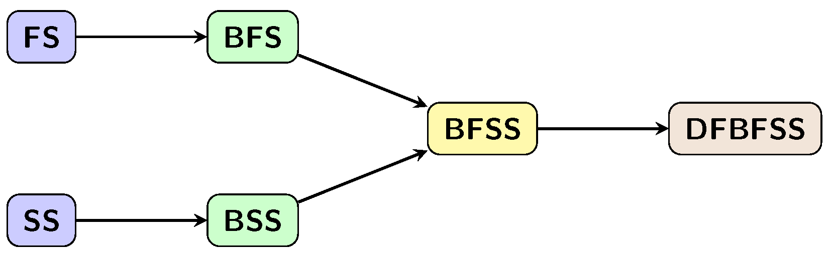
The proposed DFBFSS framework is a comprehensive generalization of established soft computing models, as it systematically reduces to them under specific constraints. By setting all negative and negation membership grades to zero, the DFBFSS simplifies to a standard fuzzy soft set (FSS), which models only positive membership. A further constraint, restricting these positive memberships to binary values $\{0,1\}$, reduces it to the classical, crisp soft set (SS). Alternatively, by merely eliminating the negation frames while retaining positive and negative memberships, the model directly becomes a bipolar fuzzy soft set (BFSS). This nested relationship solidifies the DFBFSS as a flexible and unifying superset, backward compatible with prior theories while offering superior expressiveness for complex uncertainty. The following Figure 1 justifies this generalization as follows:

1.1. Objectives

• To model complex uncertainty by using double-framing to represent both positive and negative aspects of information separately.
• To create a richer data encoding that allows information to be viewed from two competing perspectives, improving the handling of incomplete or uncertain data.
• To enable balanced multi-criteria decisions (e.g., benefit vs. cost) by providing a framework to reconcile and jointly evaluate competing objectives.
• To establish a robust decision mechanism that systematically evaluates both the positive and negative parameters of a situation.
• To apply DFBFSSs to real-world scenarios characterized by contradictory facts or dual objectives, such as risk assessment.
• To enhance decision-making in dual-objective systems, like environmental assessments (economy vs. ecology) and financial planning (profit vs. sustainability).

1.2. Research Gap and Motivation

The inspiration for DFBFSSs arises from the need to model complex decisions with conflicting, uncertain information. Unlike models that only use positive and negative memberships, the key innovation of DFBFSSs is the explicit inclusion of the negations of these membership grades. This crucial addition captures a more complete spectrum of expert judgment—such as the distinction between “not good” and “bad”—dramatically enhancing the model’s expressiveness. By separately framing membership and its negation within a double-frame structure, DFBFSSs reduce information loss and ambiguity, enabling nuanced, balanced, and more reliable decision-making in areas like healthcare, finance, and resource management where subtle trade-offs are essential.

1.3. Symmetry in the Positive–Negative Dual Framework

The double-framed architecture of DFBFSSs inherently displays a structural symmetry arising from the two parallel components that encode positive and negative membership information. Swapping these components defines an involutive transformation that preserves the overall structural behavior of the model and the fundamental operations defined on it. This symmetry highlights the balanced role of the two frames and reinforces the suitability of DFBFSSs for representing dual, mutually reflective information within complex systems.

1.4. Main Contributions

The goal of this paper is to introduce DFBFSSs as a novel, generalized framework for improving multi-criteria decision-making (MCDM) under uncertainty and conflicting criteria.

• Generalization of Models: DFBFSSs unify and extend traditional soft set models by integrating bipolarity, fuzziness, and double-framing to capture graded positive and negative assessments.
• Theoretical Foundation: We formally define DFBFSSs, establish their set-theoretic operations and algebraic properties, and build a theoretical basis for future work.
• Practical Application: We develop an MCDM algorithm based on DFBFSSs and demonstrate its effectiveness through a case study, proving its utility in real-world decision scenarios.
• Comparative Analysis: We compare the DFBFS model with existing approaches, highlighting its advantages and demonstrating its viability as a superior decision-making tool. Together, these contributions establish the DFBFS framework as a significant advancement for robust and nuanced MCDM in complex, ambiguous environments.

1.5. Structure of the Paper

This paper is structured into some sections. Section 2 is about the essential definitions of fuzzy sets, soft sets etc., and their generalized version in which we refer to some aspects related to DFBFSSs. A new framework of DFBFSSs, including its basic definitions and a few preliminary results, is presented in Section 3. This part also investigates set-theoretic operations and algebraic structures between DFBFSSs. Section 4 illustrates the use of DFBFSSs in MCDM through an algorithm used for the assessment and selection of best alternatives in decision problems. An application to model selection for searching a residential apartment to illustrate this algorithm is presented in Section 5. Results achieved by the two proposed algorithms and the reliability of results considering different techniques are compared and discussed in Section 6. Finally, Section 7 gives the summary and conclusions of the paper, including a discussion of DFBFS models’ limitations, hints for future works and possible applications of the DFBFS model and their integration with other new suggested techniques.

This paper develops a theoretical model for double-framed bipolar fuzzy soft sets (DFBFSSs) and organizes its theoretical foundations, applications, and comparative studies in a comprehensive manner, highlighting its usefulness for multi-criteria decision-making (MCDM). As is common in foundational fuzzy-set research, the focus is on theoretical model development, and real-world datasets are not included at this stage; their applicability can be demonstrated in future work.

2. Preliminaries

In order to construct the desired model, it will be helpful to keep in mind the following definitions. keep in mind the following definitions. $\Lambda$ represents the universal set, ${\rm Y}$ an entire set of parameters and $\Gamma ,\neg \Gamma \subseteq {\rm Y}$ throughout this work.

Definition 1

([39]). Let ${\rm Y}=\{{\rho }_1,{\rho }_2,\dots ,{\rho }_n\}$ be a set of parameters. Then the NOT set of Υ denoted by $\neg {\rm Y}$ is defined by $\neg {\rm Y}=\{\neg {\rho }_1,\neg {\rho }_2,\dots ,\neg {\rho }_n\}$ where $\neg {\rho }_i=$ not ${\rho }_i$ for $i=1,2,\dots ,n$.

Definition 2

([27]). A fuzzy soft set (FSS) is represented as a pair $(ð,\Gamma )$, where $ð:\Gamma \to FP(\Lambda )$ and $FP(\Lambda )$ is the collection of all fuzzy subsets of Λ.

Definition 3

([22]). A bipolar fuzzy set (BFS) $\overline{▽}$ in Λ is an object having form $\overline{▽}=\{(\varsigma ,{\wp }^{+}\left(\varsigma \right),{\wp }^{-}\left(\varsigma \right)):\forall \varsigma \in \Lambda \}$ where ${\wp }^{+}\left(\varsigma \right):\Lambda \to [0,1]$ and ${\wp }^{-}\left(\varsigma \right):\Lambda \to [-1,0]$ are indicated by the positive and negative information, respectively.

Definition 4

([31]). A triple $(\aleph ,\breve{\aleph },\Gamma )$ is called a bipolar soft set (BSS), where $\aleph :\Gamma \to P(\Lambda )$ and $\breve{\aleph }:\neg \Gamma \to P(\Lambda )$, such that $\aleph \left(\rho \right)\cap \breve{\aleph }(\neg \rho )=\varnothing$ for all $\rho \in \Gamma$ and $\neg \rho \in \neg \Gamma$.

Definition 5

([40]). A fuzzy bipolar soft set (FBSS) is represented as a triple triple $(ð,\breve{ð},\Gamma )$, where $ð:\Gamma \to FP(\Lambda )$ and $\breve{ð}:\neg \Gamma \to FP(\Lambda )$ such that $0\le ð\left(\rho \right)\left(\varsigma \right)+\breve{ð}(\neg \rho )\left(\varsigma \right)\le 1$.

Definition 6

([34]). Define $\vartheta :\Gamma \to BF(\Lambda )$, where $BF(\Lambda )$ is the collection of all bipolar fuzzy subsets of Λ. Then a pair $(\vartheta ,\Gamma )$ is said to be a bipolar fuzzy soft set (BFSS) and defined by $(\vartheta ,\Gamma )=\{(\rho ,(\varsigma ,{\varrho }^{+}\left(\varsigma \right),{\varrho }^{-}\left(\varsigma \right))):\forall \rho \in \Gamma and\forall \varsigma \in \Lambda \}$ where ${\varrho }^{+}:\Lambda ⟶[0,1]$ and ${\varrho }^{-}:\Lambda ⟶[-1,0]$ are indicated by the positive and negative information, respectively.

3. Double-Framed Bipolar Fuzzy Soft Sets (DFBFSS)

This section is focused on examining the DFBFSS concept and its basic operations as well as discussing its connection with DFBFSSs.

Definition 7.

A triple $(\vartheta ,\xi ,\Gamma )$ is called a DFBFSS over Λ where $\vartheta :\Gamma \to BF(\Lambda )$, $\xi :\neg \Gamma \to BF(\Lambda )$. A mathematical form of $(\vartheta ,\xi ,\Gamma )$ is defined by

$$\begin{array}{cc}\hfill (\vartheta ,\xi ,\Gamma )& =\left\{\right(\rho ,\vartheta \left(\rho \right),\xi (\neg \rho )):\forall \rho \in \Gamma \mathit{and}\forall \neg \rho \in \neg \Gamma \}\hfill \\ \hfill & =\left\{\left(\rho ,\left\{(\varsigma ,{\varrho }^{+}\left(\varsigma \right),{\varrho }^{-}\left(\varsigma \right))\right\},\left\{(\varsigma ,{\eta }^{+}\left(\varsigma \right),{\eta }^{-}\left(\varsigma \right))\right\}\right):\forall \rho \in \Gamma \mathit{and}\forall \varsigma \in \Lambda \right\},\hfill \end{array}$$

such that

$$0\le {\varrho }^{+}\left(\varsigma \right)+{\eta }^{+}\left(\varsigma \right)\le 1,$$

and

$$-1\le {\varrho }^{-}\left(\varsigma \right)+{\eta }^{-}\left(\varsigma \right)\le 0,$$

where ${\varrho }^{+},{\eta }^{+}:\Lambda ⟶[0,1]$ and ${\varrho }^{-},{\eta }^{-}:\Lambda ⟶[-1,0]$. The degree of satisfaction of an element ς with the property corresponding to the bipolar fuzzy set ϱ is shown by the positive and negative memberships degree ${\varrho }^{+}\left(\rho \right)\left(\varsigma \right)$ and ${\varrho }^{+}(\neg \rho )\left(\varsigma \right)$, respectively, whereas the degree of satisfaction of η with an implicit feature of η is indicated by the positive and negative membership degree ${\eta }^{+}\left(\rho \right)\left(\varsigma \right)$ and ${\eta }^{-}(\neg \rho )\left(\varsigma \right)$, respectively, with respect to ϑ and ξ.

Example 1.

Let $\Lambda =\{{\varsigma }_1,{\varsigma }_2,{\varsigma }_3\}$ be the set of three smart phones under consideration, ${\rm Y}=\{{\rho }_1=$ cheap, ${\rho }_2=$ good storage capacity, ${\rho }_3=$ high camera quality} be the set of parameters, $\neg {\rm Y}=\{\neg {\rho }_1=$ expensive, $\neg {\rho }_2=$ poor storage capacity, $\neg {\rho }_3=$ low camera quality} and $\Gamma =\{{\rho }_1,{\rho }_2\}\subseteq {\rm Y}$. Then

$$(\vartheta ,\Gamma )=\left\{\begin{array}{c}\begin{array}{c}\vartheta \left({\rho }_1\right)=\left\{\begin{array}{c}({\varsigma }_1,0.6,-0.2)\hfill \\ ({\varsigma }_2,0.3,-0.4)\hfill \\ ({\varsigma }_3,0.8,-0.3)\hfill \end{array}\right.\hfill \end{array}\hfill \\ \vartheta \left({\rho }_2\right)=\left\{\begin{array}{c}({\varsigma }_1,0.3,-0.5)\hfill \\ ({\varsigma }_2,0.7,-0.1)\hfill \\ ({\varsigma }_3,0.2,-0.2),\hfill \end{array}\right.\end{array}\right.$$

and

$$(\xi ,\neg \Gamma )=\left\{\begin{array}{c}\begin{array}{c}\xi (\neg {\rho }_1)=\left\{\begin{array}{c}({\varsigma }_1,0.3,-0.6)\hfill \\ ({\varsigma }_2,0.5,-0.2)\hfill \\ ({\varsigma }_3,0.1,-0.6)\hfill \end{array}\right.\hfill \end{array}\hfill \\ \xi (\neg {\rho }_2)=\left\{\begin{array}{c}({\varsigma }_1,0.5,-0.3)\hfill \\ ({\varsigma }_2,0.2,-0.4)\hfill \\ ({\varsigma }_3,0.4,-0.1).\hfill \end{array}\right.\hfill \end{array}\right.$$

A representative DFBFSS $(\vartheta ,\xi ,\Gamma )$ is presented in

Table 1. A DFBFSS $(\vartheta ,\xi ,\Gamma )$.

	$\mathbf{(}\mathit{\vartheta }\mathbf{,}\mathit{\Gamma }\mathbf{)}$		$\mathbf{(}\mathit{\xi }\mathbf{,}\mathbf{\neg }\mathit{\Gamma }\mathbf{)}$
	$\mathsf{\vartheta }\mathbf{\left(}{\mathsf{\rho }}_{\mathbf{1}}\mathbf{\right)}$	$\mathsf{\vartheta }\mathbf{\left(}{\mathsf{\rho }}_{\mathbf{2}}\mathbf{\right)}$	$\mathsf{\xi }\mathbf{(}\mathbf{\neg }{\mathsf{\rho }}_{\mathbf{1}}\mathbf{)}$	$\mathsf{\xi }\mathbf{(}\mathbf{\neg }{\mathsf{\rho }}_{\mathbf{2}}\mathbf{)}$
${\varsigma }_1$	$(0.6,-0.2)$	$(0.3,-0.5)$	$(0.3,-0.6)$	$(0.5,-0.3)$
${\varsigma }_2$	$(0.3,-0.4)$	$(0.7,-0.1)$	$(0.5,-0.2)$	$(0.2,-0.4)$
${\varsigma }_3$	$(0.8,-0.3)$	$(0.2,-0.2)$	$(0.1,-0.6)$	$(0.4,-0.1)$

.

To formalize the symmetry introduced in Section 1.3, we define the frame-swap operator S acting on a DFBFSS $\mathcal{F}$ by interchanging its positive and negative components. For each $\varsigma \in \Lambda$,

$$S\left(\mathcal{F}\right)\left(\varsigma \right)=\left(\mathrm{negative}\mathrm{component}\mathrm{of}\mathcal{F}\right(\varsigma ),\mathrm{positive}\mathrm{component}\mathrm{of}\mathcal{F}(\varsigma \left)\right).$$

This operator is involutive, i.e., $S\left(S\right(\mathcal{F}\left)\right)=\mathcal{F}$, and preserves the main operations of DFBFSSs, providing a formal tool to study the duality and symmetry inherent in this framework.

We emphasize that symmetry is not merely descriptive in the proposed framework, but is formalized as an algebraic invariance via a frame-swap automorphism acting on the class of DFBFSSs.

Definition 8.

Let $\mathcal{F}=(\vartheta ,\xi ,\mathsf{\Gamma })$ be a double-framed bipolar fuzzy soft set. The frame-swap operator S is defined by

$$S\left(\mathcal{F}\right)=(\xi ,\vartheta ,\mathsf{\Gamma }).$$

Proposition 1 (Symmetry Automorphism of DFBFSSs).

The frame-swap operator S is an involutive automorphism on the class of DFBFSSs, that is,

$$S^2=\mathrm{id}.$$

Moreover, S commutes with the basic operations of complement, union, and intersection.

Proof. 

By definition,

$$S\left(S\right(\vartheta ,\xi ,\mathsf{\Gamma }\left)\right)=S(\xi ,\vartheta ,\mathsf{\Gamma })=(\vartheta ,\xi ,\mathsf{\Gamma }),$$

hence $S^2=\mathrm{id}$. For each basic operation ∘, a direct verification shows that

$$S({\mathcal{F}}_1\circ {\mathcal{F}}_2)=S\left({\mathcal{F}}_1\right)\circ S\left({\mathcal{F}}_2\right),$$

which proves invariance under frame swapping.

Therefore, the collection of DFBFSSs together with the frame-swap operator S forms a structure invariant under a nontrivial involutive automorphism. □

Remark 1.

Neither BFSs nor BFSSs admit a frame-swap automorphism preserving all operations, since negation information is not explicitly encoded as an independent evaluative dimension.

Definition 9.

An absolute DFBFSS, denoted by $(\ddot{\Lambda },\ddot{\mathsf{\Phi }},\Gamma )$, is a DFBFSS $(\vartheta ,\xi ,\Gamma )$ such that $(\vartheta ,\xi ,\Gamma )=\left\{\left(\rho ,\left\{\right(\varsigma ,1,-1\left)\right\},\left\{\right(\varsigma ,0,0\left)\right\}\right):\forall \rho \in \Gamma \mathit{and}\forall \varsigma \in \Lambda \right\}$.

Definition 10.

A null DFBFSS, denoted by $(\ddot{\mathsf{\Phi }},\ddot{\Lambda },\Gamma )$, is a DFBFSS $(\vartheta ,\xi ,\Gamma )$ such that $(\vartheta ,\xi ,\Gamma )=\left\{\left(\rho ,\left\{\right(\varsigma ,0,0\left)\right\},\left\{\right(\varsigma ,1,-1\left)\right\}\right):\forall \rho \in \Gamma \mathit{and}\forall \varsigma \in \Lambda \right\}$.

Definition 11.

The DFBFS complement of $(\vartheta ,\xi ,\Gamma )$, denoted by either ${(\vartheta ,\xi ,\Gamma )}^c$ or $({\vartheta }^c,{\xi }^c,\Gamma )$, is defined by

$$\begin{array}{c}{(\vartheta ,\xi ,\Gamma )}^c=({\vartheta }^c,{\xi }^c,\Gamma )\hfill \\ =\left\{\left(\rho ,\left\{(\varsigma ,1-{\varrho }^{+}\left(\varsigma \right),{-1-\varrho }^{-}\left(\varsigma \right))\right\},\left\{(\varsigma ,1-{\eta }^{+}\left(\varsigma \right),-1-{\eta }^{-}\left(\varsigma \right))\right\}\right):\forall \rho \in \Gamma \mathrm{and}\forall \varsigma \in \Lambda \right\}.\hfill \end{array}$$

Example 2.

In Example 1, the DFBFS complement of DFBFSS $(\vartheta ,\xi ,\Gamma )$ is presented in

Table 2. A DFBFS complement ${(\vartheta ,\xi ,\Gamma )}^c$.

	${\mathbf{(}\mathit{\vartheta },\mathit{\Gamma }\mathbf{)}}^{\mathit{c}}$		${\mathbf{(}\mathit{\xi }\mathbf{,}\mathbf{\neg }\mathit{\Gamma }\mathbf{)}}^{\mathit{c}}$
	$\mathsf{\vartheta }{\mathbf{\left(}{\mathsf{\rho }}_{\mathbf{1}}\mathbf{\right)}}^{\mathit{c}}$	$\mathsf{\vartheta }{\mathbf{\left(}{\mathsf{\rho }}_{\mathbf{2}}\mathbf{\right)}}^{\mathit{c}}$	$\mathsf{\xi }{\mathbf{(}\mathbf{\neg }{\mathsf{\rho }}_{\mathbf{1}}\mathbf{)}}^{\mathit{c}}$	$\mathsf{\xi }{\mathbf{(}\mathbf{\neg }{\mathsf{\rho }}_{\mathbf{2}}\mathbf{)}}^{\mathit{c}}$
${\varsigma }_1$	$(0.4,-0.8)$	$(0.7,-0.5)$	$(0.7,-0.4)$	$(0.5,-0.7)$
${\varsigma }_2$	$(0.7,-0.6)$	$(0.3,-0.9)$	$(0.5,-0.8)$	$(0.8,-0.6)$
${\varsigma }_3$	$(0.2,-0.7)$	$(0.8,-0.8)$	$(0.9,-0.4)$	$(0.6,-0.9)$

.

Definition 12 (Subset).

Let $(\vartheta ,\xi ,\Gamma )$, $({\vartheta }_1,{\xi }_1,ß)\in$ DFBFSSs. We say that $(\vartheta ,\xi ,\Gamma )$ is an DFBFS subset of $({\vartheta }_1,{\xi }_1,ß)$, denoted as $(\vartheta ,\xi ,\Gamma )$ $\ddot{⊏}$ $({\vartheta }_1,{\xi }_1,ß)$, if

1. 

$\Gamma \subseteq ß$.

2. 

$\vartheta \left(\rho \right)\subseteq {\vartheta }_1\left(\rho \right)$ $(i.e.,$ ${{\varrho }_{\vartheta }}^{+}\left(\varsigma \right)\le {{\varrho }_{\vartheta }}_1^{+}\left(\varsigma \right),{\varrho }_{{\vartheta }^{-}}\left(\varsigma \right)\ge {{\varrho }_{\vartheta }}_1^{-}\left(\varsigma \right))$ and

$\xi (\neg \rho )\supseteq {\xi }_1(\neg \rho )$ $(i.e.,$ ${{\eta }_{\xi }}^{+}\left(\varsigma \right)\ge {{\eta }_{\xi }}_1^{+}\left(\varsigma \right),{\eta }_{{\xi }^{-}}\left(\varsigma \right)\le {{\eta }_{\xi }}_1^{-}\left(\varsigma \right))$ $\forall \rho \in \Gamma ,\forall \varsigma \in \Lambda$ and $\forall \neg \rho \in \neg \Gamma$.

Example 3.

Let $\Lambda =\{{\varsigma }_1,{\varsigma }_2,{\varsigma }_3\}$ be the set of three horses under consideration ${\rm Y}=\{{\rho }_1=$ excellent health, ${\rho }_2=$ fully trained, ${\rho }_3=$ high price, ${\rho }_4=$ high speed} be the set of parameters and $\neg {\rm Y}=\{\neg {\rho }_1=$ poor health, $\neg {\rho }_2=$ untrained, $\neg {\rho }_3=$ low price, $\neg {\rho }_4=$ low speed}. Suppose that $\Gamma =\left\{{\rho }_1\right\}$ and $ß=\{{\rho }_1,{\rho }_2\}$ are subsets of Υ. Then the representative DFBFSSs $(\vartheta ,\xi ,\Gamma )$ and $({\vartheta }_1,{\xi }_1,ß)$ are presented in

Table 3. A DFBFSS $(\vartheta ,\xi ,\Gamma )$.

	$\mathbf{(}\mathit{\vartheta }\mathbf{,}\mathit{\Gamma }\mathbf{)}$	$\mathbf{(}\mathit{\xi }\mathbf{,}\mathbf{\neg }\mathit{\Gamma }\mathbf{)}$
	$\mathsf{\vartheta }\mathbf{\left(}{\mathsf{\rho }}_{\mathbf{1}}\mathbf{\right)}$	$\mathsf{\xi }\mathbf{(}\mathbf{\neg }{\mathsf{\rho }}_{\mathbf{1}}\mathbf{)}$
${\varsigma }_1$	$(0.4,-0.1)$	$(0.3,-0.6)$
${\varsigma }_2$	$(0.3,-0.3)$	$(0.6,-0.2)$
${\varsigma }_3$	$(0.2,-0.2)$	$(0.1,-0.7)$

and

Table 4. A DFBFSS $({\vartheta }_1,{\xi }_1,ß)$.

	$\mathbf{(}{\mathit{\vartheta }}_{\mathbf{1}}\mathbf{,}\mathbf{ß}\mathbf{)}$		$\mathbf{(}{\mathit{\xi }}_{\mathbf{1}},\mathbf{\neg }\mathbf{ß}\mathbf{)}$
	${\mathsf{\vartheta }}_{\mathbf{1}}\mathbf{\left(}{\mathsf{\rho }}_{\mathbf{1}}\mathbf{\right)}$	${\mathsf{\vartheta }}_{\mathbf{1}}\mathbf{\left(}{\mathsf{\rho }}_{\mathbf{2}}\mathbf{\right)}$	${\mathsf{\xi }}_{\mathbf{1}}\mathbf{(}\mathbf{\neg }{\mathsf{\rho }}_{\mathbf{1}}\mathbf{)}$	${\mathsf{\xi }}_{\mathbf{1}}\mathbf{(}\mathbf{\neg }{\mathsf{\rho }}_{\mathbf{2}}\mathbf{)}$
${\varsigma }_1$	$(0.7,-0.2)$	$(0.3,-0.5)$	$(0.3,-0.6)$	$(0.5,-0.3)$
${\varsigma }_2$	$(0.4,-0.4)$	$(0.6,-0.1)$	$(0.5,-0.2)$	$(0.2,-0.4)$
${\varsigma }_3$	$(0.9,-0.5)$	$(0.1,-0.2)$	$(0.1,-0.6)$	$(0.4,-0.1)$

, respectively.

Then (1.) $\Gamma \subseteq ß$, (2.) $\forall \rho \in \Gamma ,\forall \varsigma \in \Lambda$ and $\forall \neg \rho \in \neg \Gamma$, we have $\vartheta \left(\rho \right)\subseteq {\vartheta }_1\left(\rho \right)$ and $\xi (\neg \rho )\supseteq {\xi }_1(\neg \rho )$. Therefore, $(\vartheta ,\xi ,\Gamma )$ $\ddot{⊏}$ $({\vartheta }_1,{\xi }_1,ß)$.

Definition 13 (Equal).

Two DFBFSSs $(\vartheta ,\xi ,\Gamma )$ and $({\vartheta }_1,{\xi }_1,ß)$ are said to be DFBFS equal if $({\vartheta }_1,{\xi }_1,ß)\ddot{⊏}(\vartheta ,\xi ,\Gamma )$ and $(\vartheta ,\xi ,\Gamma )\ddot{⊏}({\vartheta }_1,{\xi }_1,ß)$. We write $({\vartheta }_1,{\xi }_1,ß)=(\vartheta ,\xi ,\Gamma )$.

4. Operations on DFBFSSs

Definition 14

(OR). The DFBFS OR-operation of $(\vartheta ,\xi ,\Gamma )$ and $({\vartheta }_1,{\xi }_1,ß)$ is a DFBFSS $(\mathsf{\mho },\mathsf{\Omega },\hslash )$, denoted by $(\vartheta ,\xi ,\Gamma )$ $\ddot{\vee }$ $({\vartheta }_1,{\xi }_1,ß)$, and is defined as $(\vartheta ,\xi ,\Gamma )$ $\ddot{\vee }$ $({\vartheta }_1,{\xi }_1,ß)=(\mathsf{\mho },\mathsf{\Omega },\Gamma \times ß)$ where $\forall (\gamma ,\mathsf{ȷ})\in \Gamma \times ß$, $(\neg \gamma ,\neg \mathsf{ȷ})\in \neg \Gamma \times \neg ß$ and $\varsigma \in \Lambda$,

$$\begin{array}{cc}\hfill \mathsf{\mho }(\gamma ,\mathsf{ȷ})=& ({{\varrho }_{\vartheta }}^{+}\left(\varsigma \right)\vee {{\varrho }_{\vartheta }}_1^{+}\left(\varsigma \right),{{\varrho }_{\vartheta }}^{-}\left(\varsigma \right)\wedge {{\varrho }_{\vartheta }}_1^{-}\left(\varsigma \right))and\hfill \\ \hfill \mathsf{\Omega }(\neg \gamma ,\neg \mathsf{ȷ})=& ({\eta }_{{\xi }^{+}}\left(\varsigma \right)\wedge {{\eta }_{\xi }}_1^{+}\left(\varsigma \right),{{\eta }_{\xi }}^{-}\left(\varsigma \right)\vee {{\eta }_{\xi }}_1^{-}\left(\varsigma \right)).\hfill \end{array}$$

Example 4.

In Example 3, $(\mathsf{\mho },\mathsf{\Omega },\Gamma \times ß)=(\vartheta ,\xi ,\Gamma )$ $\ddot{\vee }$ $({\vartheta }_1,{\xi }_1,ß)$. The representative DFBFSS $(\vartheta ,\xi ,\Gamma )$ $\ddot{\vee }$ $({\vartheta }_1,{\xi }_1,ß)$ is presented in

Table 5. $(\vartheta ,\xi ,\Gamma )$ $\ddot{\vee }$ $({\vartheta }_1,{\xi }_1,ß)$.

	$\mathsf{\mho }\mathbf{(}{\mathit{\rho }}_{\mathbf{1}}\mathbf{,}{\mathit{\rho }}_{\mathbf{1}}\mathbf{)}$	$\mathsf{\mho }\mathbf{(}{\mathit{\rho }}_{\mathbf{1}}\mathbf{,}{\mathit{\rho }}_{\mathbf{2}}\mathbf{)}$	$\mathsf{\Omega }\mathbf{(}\mathbf{\neg }{\mathit{\rho }}_{\mathbf{1}}\mathbf{,}\mathbf{\neg }{\mathit{\rho }}_{\mathbf{1}}\mathbf{)}$	$\mathsf{\Omega }\mathbf{(}\mathbf{\neg }{\mathit{\rho }}_{\mathbf{1}}\mathbf{,}\mathbf{\neg }{\mathit{\rho }}_{\mathbf{2}}\mathbf{)}$
${\varsigma }_1$	$(0.7,-0.2)$	$(0.4,-0.5)$	$(0.3,-0.6)$	$(0.3,-0.3)$
${\varsigma }_2$	$(0.4,-0.4)$	$(0.6,-0.3)$	$(0.5,-0.2)$	$(0.2,-0.2)$
${\varsigma }_3$	$(0.9,-0.5)$	$(0.2,-0.2)$	$(0.1,-0.6)$	$(0.1,-0.1)$

.

Definition 15

(AND). The DFBFS AND-operation of $(\vartheta ,\xi ,\Gamma )$ and $({\vartheta }_1,{\xi }_1,ß)$ is a DFBFSS $(\mathsf{\mho },\mathsf{\Omega },\hslash )$, denoted by $(\vartheta ,\xi ,\Gamma )$ $\ddot{\wedge }$ $({\vartheta }_1,{\xi }_1,ß)$, and is defined by $(\vartheta ,\xi ,\Gamma )$ $\ddot{\wedge }$ $({\vartheta }_1,{\xi }_1,ß)=(\mathsf{\mho },\mathsf{\Omega },\Gamma \times ß)$ where $\forall (\gamma ,\mathsf{ȷ})$∈$\Gamma \times ß$, $(\neg \gamma ,\neg \mathsf{ȷ})\in \neg \Gamma \times \neg ß$ and $\varsigma \in \Lambda$,

$$\begin{array}{cc}\hfill \mathsf{\mho }(\gamma ,\mathsf{ȷ})=& ({{\varrho }_{\vartheta }}^{+}\left(\varsigma \right)\wedge {{\varrho }_{\vartheta }}_1^{+}\left(\varsigma \right),{{\varrho }_{\vartheta }}^{-}\left(\varsigma \right)\vee {{\varrho }_{\vartheta }}_1^{-}\left(\varsigma \right))and\hfill \\ \hfill \mathsf{\Omega }(\neg \gamma ,\neg \mathsf{ȷ})=& ({{\eta }_{\xi }}^{+}\left(\varsigma \right)\vee {{\eta }_{\xi }}_1^{+}\left(\varsigma \right),{{\eta }_{\xi }}^{-}\left(\varsigma \right)\wedge {{\eta }_{\xi }}_1^{-}\left(\varsigma \right)).\hfill \end{array}$$

Example 5.

In Example 3, $(\mathsf{\mho },\mathsf{\Omega },\Gamma \times ß)=(\vartheta ,\xi ,\Gamma )$ $\ddot{\wedge }$ $({\vartheta }_1,{\xi }_1,ß)$. The representative DFBFSS $(\vartheta ,\xi ,\Gamma )$ $\ddot{\wedge }$ $({\vartheta }_1,{\xi }_1,ß)$ is presented in

Table 6. $(\vartheta ,\xi ,\Gamma )$ $\ddot{\wedge }$ $({\vartheta }_1,{\xi }_1,ß)$.

	$\mathsf{\mho }\mathbf{(}{\mathit{\rho }}_{\mathbf{1}}\mathbf{,}{\mathit{\rho }}_{\mathbf{1}}\mathbf{)}$	$\mathsf{\mho }\mathbf{(}{\mathit{\rho }}_{\mathbf{1}}\mathbf{,}{\mathit{\rho }}_{\mathbf{2}}\mathbf{)}$	$\mathsf{\Omega }\mathbf{(}\mathbf{\neg }{\mathit{\rho }}_{\mathbf{1}}\mathbf{,}\mathbf{\neg }{\mathit{\rho }}_{\mathbf{1}}\mathbf{)}$	$\mathsf{\Omega }\mathbf{(}\mathbf{\neg }{\mathit{\rho }}_{\mathbf{1}}\mathbf{,}\mathbf{\neg }{\mathit{\rho }}_{\mathbf{2}}\mathbf{)}$
${\varsigma }_1$	$(0.4,-0.1)$	$(0.3,-0.1)$	$(0.3,-0.6)$	$(0.5,-0.6)$
${\varsigma }_2$	$(0.3,-0.3)$	$(0.3,-0.1)$	$(0.6,-0.2)$	$(0.6,-0.4)$
${\varsigma }_3$	$(0.2,-0.2)$	$(0.1,-0.2)$	$(0.1,-0.7)$	$(0.4,-0.7)$

.

Proposition 2.

If $(\vartheta ,\xi ,\Gamma )$ and $({\vartheta }_1,{\xi }_1,ß)$ are two DFBFSSs over Λ, then

1. 

$\left(\right(\vartheta ,\xi ,\Gamma )$ $\ddot{\vee }$ $({\vartheta }_1,{\xi }_1,ß){)}^c={(\vartheta ,\xi ,\Gamma )}^c$ $\ddot{\wedge }$ ${({\vartheta }_1,{\xi }_1,ß)}^c$.

2. 

$\left(\right(\vartheta ,\xi ,\Gamma )$ $\ddot{\wedge }$ $({\vartheta }_1,{\xi }_1,ß){)}^c={(\vartheta ,\xi ,\Gamma )}^c$ $\ddot{\vee }$ ${({\vartheta }_1,{\xi }_1,ß)}^c$.

Proof. 

1. From Definitions 11 and 14, $\left(\right(\vartheta ,\xi ,\Gamma )$ $\ddot{\vee }$ $({\vartheta }_1,{\xi }_1,ß){)}^c=({\mathsf{\mho }}^c,{\mathsf{\Omega }}^c,\Gamma \times ß)$, where $\mathsf{\mho }{(\gamma ,\mathsf{ȷ})}^c=\vartheta {\left(\gamma \right)}^c\wedge {\vartheta }_1{\left(\mathsf{ȷ}\right)}^c$ and $\mathsf{\Omega }{(\neg \gamma ,\neg \mathsf{ȷ})}^c=\xi {(\neg \gamma )}^c\vee {\xi }_1{(\neg \mathsf{ȷ})}^c$ for all $(\gamma ,\mathsf{ȷ})\in \Gamma \times ß$ and $(\neg \gamma ,\neg \mathsf{ȷ})\in \neg \Gamma \times \neg ß$.

• Now, ${(\vartheta ,\xi ,\Gamma )}^c$ $\ddot{\wedge }$ ${({\vartheta }_1,{\xi }_1,ß)}^c=({\mathsf{\mho }}^c,{\mathsf{\Omega }}^c,\Gamma \times ß)$ where $\mathsf{\mho }{(\gamma ,\mathsf{ȷ})}^c=\vartheta {\left(\gamma \right)}^c\wedge {\vartheta }_1{\left(\mathsf{ȷ}\right)}^c$ and $\mathsf{\Omega }{(\neg \gamma ,\neg \mathsf{ȷ})}^c=\xi {(\neg \gamma )}^c\vee {\xi }_1{(\neg \mathsf{ȷ})}^c$ for all $(\gamma ,\mathsf{ȷ})\in \Gamma \times ß$ and $(\neg \gamma ,\neg \mathsf{ȷ})\in \neg \Gamma \times \neg ß$. Thus, $\left(\right(\vartheta ,\xi ,\Gamma )$ $\ddot{\vee }$ $({\vartheta }_1,{\xi }_1,ß){)}^c={(\vartheta ,\xi ,\Gamma )}^c$ $\ddot{\wedge }$ ${({\vartheta }_1,{\xi }_1,ß)}^c$.

2.

Its proof is similar to part 1.

□

Definition 16

(Extended union). The DFBFS extended union of $(\vartheta ,\xi ,\Gamma )$ and $({\vartheta }_1,{\xi }_1,ß)$, denoted by $(\vartheta ,\xi ,\Gamma )$ $\ddot{\bigsqcup }$ $({\vartheta }_1,{\xi }_1,ß)$, is a DFBFSS $(\mathsf{\mho },\mathsf{\Omega },\hslash )$ where $\hslash =\Gamma \cup ß$ and $\forall \rho \in \hslash$:

$$\begin{array}{cc}\hfill \mathsf{\mho }\left(\rho \right)& =\left\{\begin{array}{c}\vartheta \left(\rho \right)\mathit{if}\rho \in \Gamma \setminus ß\hfill \\ {\vartheta }_1\left(\rho \right)\mathit{if}\rho \in ß\setminus \Gamma \hfill \\ \vartheta \left(\rho \right)\ddot{\vee }{\vartheta }_1\left(\rho \right)\mathit{if}\rho \in \Gamma \cap ß\ne \varnothing ,\hfill \end{array}\right.\hfill \end{array}$$

and

$$\begin{array}{cc}\hfill \mathsf{\Omega }(\neg \rho )& =\left\{\begin{array}{c}\xi (\neg \rho )\mathit{if}\neg \rho \in \neg \Gamma \setminus \neg ß\hfill \\ {\xi }_1(\neg \rho )\mathit{if}\neg \rho \in \neg ß\setminus \neg \Gamma \hfill \\ \xi (\neg \rho )\ddot{\wedge }{\xi }_1(\neg \rho )\mathit{if}\neg \rho \in \neg \Gamma \cap \neg ß\ne \varnothing .\hfill \end{array}\right.\hfill \end{array}$$

Example 6.

In Example 3, $(\mathsf{\mho },\mathsf{\Omega },\hslash )=(\vartheta ,\xi ,\Gamma )$ $\ddot{\bigsqcup }$ $({\vartheta }_1,{\xi }_1,ß)$, where $\hslash =\Gamma \cup ß=\{{\rho }_1,{\rho }_2\}$. The representative DFBFSS $(\vartheta ,\xi ,\Gamma )$ $\ddot{\bigsqcup }$ $({\vartheta }_1,{\xi }_1,ß)$ is presented in

Table 7. $(\vartheta ,\xi ,\Gamma )$ $\ddot{\bigsqcup }$ $({\vartheta }_1,{\xi }_1,ß)$.

	$\mathbf{(}\mathsf{\mho }\mathbf{,}\mathit{\hslash }\mathbf{)}$		$\mathbf{(}\mathsf{\Omega }\mathbf{,}\mathbf{\neg }\mathit{\hslash }\mathbf{)}$
	$\mathsf{\mho }\mathbf{\left(}{\mathsf{\rho }}_{\mathbf{1}}\mathbf{\right)}$	$\mathsf{\mho }\mathbf{\left(}{\mathsf{\rho }}_{\mathbf{2}}\mathbf{\right)}$	$\mathsf{\Omega }\mathbf{(}\mathbf{\neg }{\mathbf{\rho }}_{\mathbf{1}}\mathbf{)}$	$\mathsf{\Omega }\mathbf{(}\mathbf{\neg }{\mathsf{\rho }}_{\mathbf{2}}\mathbf{)}$
${\varsigma }_1$	$(0.7,-0.2)$	$(0.3,-0.5)$	$(0.3,-0.6)$	$(0.5,-0.3)$
${\varsigma }_2$	$(0.4,-0.4)$	$(0.6,-0.1)$	$(0.5,-0.2)$	$(0.2,-0.4)$
${\varsigma }_3$	$(0.9,-0.5)$	$(0.1,-0.2)$	$(0.1,-0.6)$	$(0.4,-0.1)$

.

Definition 17

(Extended intersection). The DFBFS extended intersection of $(\vartheta ,\xi ,\Gamma )$ and $({\vartheta }_1,{\xi }_1,ß)$, denoted by $(\mathsf{\mho },\mathsf{\Omega },\hslash )=(\vartheta ,\xi ,\Gamma )$ $\ddot{\sqcap }$ $({\vartheta }_1,{\xi }_1,ß)$, is a DFBFSS $(\mathsf{\mho },\mathsf{\Omega },\hslash )$, where $\hslash =\Gamma \cup ß$ and $\forall \rho \in \hslash$:

$$\begin{array}{cc}\hfill \mathsf{\mho }\left(\rho \right)& =\left\{\begin{array}{c}\vartheta \left(\rho \right)\mathit{if}\rho \in \Gamma \setminus ß\hfill \\ {\vartheta }_1\left(\rho \right)\mathit{if}\rho \in ß\setminus \Gamma \hfill \\ \vartheta \left(\rho \right)\ddot{\wedge }{\vartheta }_1\left(\rho \right)\mathit{if}\rho \in \Gamma \cap ß\ne \varnothing ,\hfill \end{array}\right.\hfill \end{array}$$

and

$$\begin{array}{cc}\hfill \mathsf{\Omega }(\neg \rho )& =\left\{\begin{array}{c}\xi (\neg \rho )\mathit{if}\neg \rho \in \neg \Gamma \setminus \neg ß\hfill \\ {\xi }_1(\neg \rho )\mathit{if}\neg \rho \in \neg ß\setminus \neg \Gamma \hfill \\ \xi (\neg \rho )\ddot{\vee }{\xi }_1(\neg \rho )\mathit{if}\neg \rho \in \neg \Gamma \cap \neg ß\ne \varnothing .\hfill \end{array}\right.\hfill \end{array}$$

Example 7.

In Example 3, $(\mathsf{\mho },\mathsf{\Omega },\hslash )=(\vartheta ,\xi ,\Gamma )$ $\ddot{\sqcap }$ $({\vartheta }_1,{\xi }_1,ß)$, where $\hslash =\Gamma \cup ß=\{{\rho }_1,{\rho }_2\}$. The representative DFBFSS $(\vartheta ,\xi ,\Gamma )$ $\ddot{\sqcap }$ $({\vartheta }_1,{\xi }_1,ß)$ is presented in

Table 8. $(\vartheta ,\xi ,\Gamma )$ $\ddot{\sqcap }$ $({\vartheta }_1,{\xi }_1,ß)$.

	$\mathbf{(}\mathsf{\mho }\mathbf{,}\mathsf{\hslash }\mathbf{)}$		$\mathbf{(}\mathsf{\Omega }\mathbf{,}\mathbf{\neg }\mathit{\hslash }\mathbf{)}$
	$\mathsf{\mho }\mathbf{\left(}{\mathsf{\rho }}_{\mathbf{1}}\mathbf{\right)}$	$\mathsf{\mho }\mathbf{\left(}{\mathsf{\rho }}_{\mathbf{2}}\mathbf{\right)}$	$\mathsf{\Omega }\mathbf{(}\mathbf{\neg }{\mathsf{\rho }}_{\mathbf{1}}\mathbf{)}$	$\mathsf{\Omega }\mathbf{(}\mathbf{\neg }{\mathsf{\rho }}_{\mathbf{2}}\mathbf{)}$
${\varsigma }_1$	$(0.4,-0.1)$	$(0.3,-0.5)$	$(0.3,-0.6)$	$(0.5,-0.3)$
${\varsigma }_2$	$(0.3,-0.3)$	$(0.6,-0.1)$	$(0.6,-0.2)$	$(0.2,-0.4)$
${\varsigma }_3$	$(0.2,-0.2)$	$(0.1,-0.2)$	$(0.1,-0.7)$	$(0.4,-0.1)$

.

Definition 18

(Restricted union). The DFBFS restricted union of $(\vartheta ,\xi ,\Gamma )$ and $({\vartheta }_1,{\xi }_1,ß)$, denoted by $(\vartheta ,\xi ,\Gamma ){\bigsqcup }_{\Re }({\vartheta }_1,{\xi }_1,ß)$, is a DFBFSSs $(\mathsf{\mho },\mathsf{\Omega },\hslash )$, where $\hslash =\Gamma \cap ß\ne \varnothing$ and $\forall \rho \in \hslash$,

$$\begin{array}{c}\hfill \mathsf{\mho }\left(\rho \right)=\vartheta \left(\rho \right)\ddot{\vee }{\vartheta }_1\left(\rho \right)\mathit{and}\mathsf{\Omega }(\neg \rho )=\xi (\neg \rho )\ddot{\wedge }{\xi }_1(\neg \rho ).\end{array}$$

Example 8.

In Example 3, $(\mathsf{\mho },\mathsf{\Omega },\hslash )=(\vartheta ,\xi ,\Gamma )$ ${\bigsqcup }_{\Re }$ $({\vartheta }_1,{\xi }_1,ß)$ where $\hslash =A\cap B=\left\{{\rho }_1\right\}$. The representative DFBFSS $(\vartheta ,\xi ,\Gamma )$ ${\bigsqcup }_{\Re }$ $({\vartheta }_1,{\xi }_1,ß)$ is presented in

Table 9. $(\vartheta ,\xi ,\Gamma )$ ${\bigsqcup }_{\Re }$ $({\vartheta }_1,{\xi }_1,ß)$.

	$\mathbf{(}\mathsf{\mho }\mathbf{,}\mathit{\hslash }\mathbf{)}$	$\mathbf{(}\mathsf{\Omega }\mathbf{,}\mathbf{\neg }\mathit{\hslash }\mathbf{)}$
	$\mathsf{\mho }\mathbf{\left(}{\mathsf{\rho }}_{\mathbf{1}}\mathbf{\right)}$	$\mathsf{\Omega }\mathbf{(}\mathbf{\neg }{\mathsf{\rho }}_{\mathbf{1}}\mathbf{)}$
${\varsigma }_1$	$(0.7,-0.2)$	$(0.3,-0.6)$
${\varsigma }_2$	$(0.4,-0.4)$	$(0.5,-0.2)$
${\varsigma }_3$	$(0.9,-0.5)$	$(0.1,-0.6)$

.

Definition 19

(Restricted intersection). The DFBFS restricted intersection of $(\vartheta ,\xi ,\Gamma )$ and $({\vartheta }_1,{\xi }_1,ß)$, denoted by $(\vartheta ,\xi ,\Gamma )$ ${\sqcap }_{\Re }$ $({\vartheta }_1,{\xi }_1,ß)$, is a DFBFSSs $(\mathsf{\mho },\mathsf{\Omega },\hslash )$, where $\hslash =\Gamma \cap ß\ne \varnothing$ and $\forall \rho \in \hslash$,

$$\begin{array}{c}\hfill \mathsf{\mho }\left(\rho \right)=\vartheta \left(\rho \right)\ddot{\wedge }{\vartheta }_1\left(\rho \right)\mathit{and}\mathsf{\Omega }(\neg \rho )=\xi (\neg \rho )\ddot{\vee }{\xi }_1(\neg \rho ).\end{array}$$

Example 9.

In Example 3, $(\mathsf{\mho },\mathsf{\Omega },\hslash )=(\vartheta ,\xi ,\Gamma )$ ${\sqcap }_{\Re }$ $({\vartheta }_1,{\xi }_1,ß)$, where $\hslash =A\cap B=\left\{{\rho }_1\right\}$. The representative DFBFSS $(\vartheta ,\xi ,\Gamma )$ ${\sqcap }_{\Re }$ $({\vartheta }_1,{\xi }_1,ß)$ is presented in

Table 10. $(\vartheta ,\xi ,\Gamma )$ ${\sqcap }_{\Re }$ $({\vartheta }_1,{\xi }_1,ß)$.

	$\mathbf{(}\mathsf{\mho }\mathbf{,}\mathit{\hslash }\mathbf{)}$	$\mathbf{(}\mathsf{\Omega }\mathbf{,}\mathbf{\neg }\mathit{\hslash }\mathbf{)}$
	$\mathsf{\mho }\mathbf{\left(}{\mathsf{\rho }}_{\mathbf{1}}\mathbf{\right)}$	$\mathsf{\Omega }\mathbf{(}\mathbf{\neg }{\mathsf{\rho }}_{\mathbf{1}}\mathbf{)}$
${\varsigma }_1$	$(0.4,-0.1)$	$(0.3,-0.6)$
${\varsigma }_2$	$(0.3,-0.3)$	$(0.6,-0.2)$
${\varsigma }_3$	$(0.2,-0.2)$	$(0.1,-0.7)$

.

Proposition 3.

Let $(\vartheta ,\xi ,\Gamma )$, $({\vartheta }_1,{\xi }_1,ß)$, $({\vartheta }_2,{\xi }_2,\hslash )\in DFBFSS(\Lambda )$. Then

1. 

${(\ddot{\Lambda },\ddot{\mathsf{\Phi }},\Gamma )}^c=(\ddot{\mathsf{\Phi }},\ddot{\Lambda },\Gamma )$ and ${(\ddot{\mathsf{\Phi }},\ddot{\Lambda },\Gamma )}^c=(\ddot{\Lambda },\ddot{\mathsf{\Phi }},\Gamma )$.

2. 

$(\ddot{\mathsf{\Phi }},\ddot{\Lambda },\Gamma )\ddot{\sqcap }(\vartheta ,\xi ,\Gamma )=(\ddot{\mathsf{\Phi }},\ddot{\Lambda },\Gamma )$ and $(\ddot{\mathsf{\Phi }},\ddot{\Lambda },\Gamma )\ddot{\bigsqcup }(\vartheta ,\xi ,\Gamma )=(\vartheta ,\xi ,\Gamma )$.

3. 

$(\ddot{\Lambda },\ddot{\mathsf{\Phi }},\Gamma ){\sqcap }_{\Re }(\vartheta ,\xi ,\Gamma )=(\ddot{\mathsf{\Phi }},\ddot{\Lambda },\Gamma )$ and $(\ddot{\mathsf{\Phi }},\ddot{\Lambda },\Gamma ){\bigsqcup }_{\Re }(\vartheta ,\xi ,\Gamma )=(\vartheta ,\xi ,\Gamma )$.

4. 

$(\ddot{\mathsf{\Phi }},\ddot{\Lambda },\Gamma )\ddot{⊏}(\vartheta ,\xi ,\Gamma )$.

5. 

$(\vartheta ,\xi ,\Gamma )\ddot{⊏}(\ddot{\Lambda },\ddot{\mathsf{\Phi }},\Gamma )$.

6. 

${\left({(\vartheta ,\xi ,\Gamma )}^c\right)}^c=(\vartheta ,\xi ,\Gamma )$.

7. 

If $(\vartheta ,\xi ,\Gamma )$ $\ddot{⊏}$ $({\vartheta }_1,{\xi }_1,ß)$, then ${({\vartheta }_1,{\xi }_1,ß)}^c$ $\ddot{⊏}$ ${(\vartheta ,\xi ,\Gamma )}^c$.

8. 

If $(\vartheta ,\xi ,\Gamma )$ $\ddot{⊏}$ $({\vartheta }_1,{\xi }_1,ß)$, then $(\vartheta ,\xi ,\Gamma )$ $\ddot{\bigsqcup }$ $({\vartheta }_1,{\xi }_1,ß)=({\vartheta }_1,{\xi }_1,ß)$.

9. 

If $(\vartheta ,\xi ,\Gamma )$ $\ddot{⊏}$ $({\vartheta }_1,{\xi }_1,ß)$, then $(\vartheta ,\xi ,\Gamma )$ ${\sqcap }_{\Re }$ $({\vartheta }_1,{\xi }_1,ß)=(\vartheta ,\xi ,\Gamma )$.

10. 

If $(\vartheta ,\xi ,\Gamma )$ $\ddot{⊏}$ $({\vartheta }_1,{\xi }_1,ß)$ and $({\vartheta }_1,{\xi }_1,ß)$ $\ddot{⊏}$ $({\vartheta }_2,{\xi }_2,\hslash )$, then $(\vartheta ,\xi ,\Gamma )$ $\ddot{⊏}$ $({\vartheta }_2,{\xi }_2,\hslash )$.

Proof. 

(1) Let, for simplicity $(\ddot{\Lambda },\ddot{\mathsf{\Phi }},\Gamma )=\left((1,-1),(0,0)\right)$. Then

• ${(\ddot{\Lambda },\ddot{\mathsf{\Phi }},\Gamma )}^c=\left((1-1,-1-(-1\left)\right),(1-0,-1-0)\right)=\left((0,0),(1,-1)\right)=(\ddot{\mathsf{\Phi }},\ddot{\Lambda },\Gamma )$ and ${(\ddot{\mathsf{\Phi }},\ddot{\Lambda },\Gamma )}^c=(\ddot{\Lambda },\ddot{\mathsf{\Phi }},\Gamma )$ is similar to above.

The proofs of 2–5 can be directly proven from their definitions.

(6)

Let, for simplicity, $(\vartheta ,\xi ,\Gamma )=\left(({\varrho }^{+},{\varrho }^{-}),({\eta }^{+},{\eta }^{-})\right)$. Then ${(\vartheta ,\xi ,\Gamma )}^c=\left((1-{\varrho }^{+},-1-{\varrho }^{-}),(1-{\eta }^{+},-1-{\eta }^{-})\right)$ and

$$\begin{array}{cc}\hfill {\left({(\vartheta ,\xi ,\Gamma )}^c\right)}^c& =\left(1-(1-{\varrho }^{+}),-1-(-1-{\varrho }^{-}),1-(1-{\eta }^{+}),-1-(-1-{\eta }^{-})\right)\hfill \\ \hfill & =(\vartheta ,\xi ,\Gamma ).\hfill \end{array}$$

(7)

Since $(\vartheta ,\xi ,\Gamma )$ $\ddot{⊏}$ $({\vartheta }_1,{\xi }_1,ß)$, it follows that $\Gamma \subseteq ß$ and $\vartheta \left(\rho \right)\subseteq {\vartheta }_1\left(\rho \right)$ and $\xi (\neg \rho )\supseteq {\xi }_1(\neg \rho )$ $\forall \rho \in \Gamma$. Then, $({{\vartheta }_1}^c,{{\xi }_1}^c,ß)\ddot{⊏}({\vartheta }^c,{\xi }^c,\Gamma )$. Hence, ${({\vartheta }_1,{\xi }_1,ß)}^c$ $\ddot{⊏}$ ${(\vartheta ,\xi ,\Gamma )}^c$.

(8)

Since $(\vartheta ,\xi ,\Gamma )$ $\ddot{⊏}$ $({\vartheta }_1,{\xi }_1,ß)$, it follows that $\Gamma \subseteq ß$ and $\vartheta \left(\rho \right)\subseteq {\vartheta }_1\left(\rho \right)$ and $\xi (\neg \rho )\supseteq {\xi }_1(\neg \rho )$ $\forall \rho \in \Gamma$. Put $(\mathsf{\mho },\mathsf{\Omega },\hslash )=(\vartheta ,\xi ,\Gamma )$ $\ddot{\bigsqcup }$ $({\vartheta }_1,{\xi }_1,ß)$. Then $\hslash =\Gamma \cup ß$ and $\forall \rho \in \hslash =ß$,

$$\begin{array}{cc}\hfill \mathsf{\mho }\left(\rho \right)& =\left\{\begin{array}{c}{\vartheta }_1\left(\rho \right)\mathrm{if}\rho \in ß\setminus \Gamma \hfill \\ \vartheta \left(\rho \right)\ddot{\vee }{\vartheta }_1\left(\rho \right)\mathrm{if}\rho \in \Gamma \cap ß\ne \varnothing ,\hfill \end{array}\right.\hfill \end{array}$$

and

$$\begin{array}{cc}\hfill \mathsf{\Omega }(\neg \rho )& =\left\{\begin{array}{c}{\xi }_1(\neg \rho )\mathrm{if}\neg \rho \in \neg ß\setminus \neg \Gamma \hfill \\ \xi (\neg \rho )\ddot{\wedge }{\xi }_1(\neg \rho )\mathrm{if}\neg \rho \in \neg \Gamma \cap \neg ß\ne \varnothing .\hfill \end{array}\right.\hfill \end{array}$$

Then $(\mathsf{\mho },\mathsf{\Omega },\hslash )=({\vartheta }_1,{\xi }_1,ß)$. Thus $(\vartheta ,\xi ,\Gamma )$ $\ddot{\bigsqcup }$ $({\vartheta }_1,{\xi }_1,ß)=({\vartheta }_1,{\xi }_1,ß)$.

(9)

Since $(\vartheta ,\xi ,\Gamma )$ $\ddot{⊏}$ $({\vartheta }_1,{\xi }_1,ß)$, it follows that $\Gamma \subseteq ß$, $\vartheta \left(\rho \right)\subseteq {\vartheta }_1\left(\rho \right)$ and $\xi (\neg \rho )\supseteq {\xi }_1(\neg \rho )$ $\forall \rho \in \Gamma$. Put $(\mathsf{\mho },\mathsf{\Omega },\hslash )=(\vartheta ,\xi ,\Gamma )$ ${\sqcap }_{\Re }$ $({\vartheta }_1,{\xi }_1,ß)$. Then $\hslash =\Gamma \cap ß\ne \varnothing$ and $\forall \rho \in \hslash =\Gamma$,

$$\begin{array}{c}\hfill \mathsf{\mho }\left(\rho \right)=\vartheta \left(\rho \right)\mathrm{and}\mathsf{\Omega }(\neg \rho )=\xi (\neg \rho ).\end{array}$$

Then $(\mathsf{\mho },\mathsf{\Omega },\hslash )=(\vartheta ,\xi ,\Gamma ).$ Thus $(\vartheta ,\xi ,\Gamma )$ ${\sqcap }_{\Re }$ $({\vartheta }_1,{\xi }_1,ß)=(\vartheta ,\xi ,\Gamma )$.

(10)

Since $(\vartheta ,\xi ,\Gamma )$ $\ddot{⊏}$ $({\vartheta }_1,{\xi }_1,ß)$ and $({\vartheta }_1,{\xi }_1,ß)$ $\ddot{⊏}$ $({\vartheta }_2,{\xi }_2,\hslash )$, it follows that $\Gamma \subseteq ß$, $ß\subseteq \hslash$ and $\vartheta \left(\rho \right)\subseteq {\vartheta }_1\left(\rho \right)$, ${\vartheta }_1\left(\rho \right)\subseteq {\vartheta }_2\left(\rho \right)$ and $\xi (\neg \rho )\supseteq {\xi }_1(\neg \rho )$, ${\xi }_1(\neg \rho )\supseteq {\xi }_2(\neg \rho )$ $\forall \rho \in \Gamma .$ Therefore, $\Gamma \subseteq \hslash$, $\vartheta \left(\rho \right)\subseteq {\vartheta }_2\left(\rho \right)$ and $\xi (\neg \rho )\supseteq {\xi }_2(\neg \rho )$. Hence, $(\vartheta ,\xi ,\Gamma )$ $\ddot{⊏}$ $({\vartheta }_2,{\xi }_2,\hslash )$.   □

Proposition 4.

Let $(\vartheta ,\xi ,\Gamma )$, $({\vartheta }_1,{\xi }_1,ß)\in DFBFSS(\Lambda )$. Then the De-Morgan’s law of $(\vartheta ,\xi ,\Gamma )$ and $({\vartheta }_1,{\xi }_1,ß)$ is as follows:

1. 

$\left(\right(\vartheta ,\xi ,\Gamma )$ $\ddot{\bigsqcup }$ $({\vartheta }_1,{\xi }_1,ß){)}^c={(\vartheta ,\xi ,\Gamma )}^c$ $\ddot{\sqcap }$ ${({\vartheta }_1,{\xi }_1,ß)}^c$.

2. 

$\left(\right(\vartheta ,\xi ,\Gamma )$ $\ddot{\sqcap }$ $({\vartheta }_1,{\xi }_1,ß){)}^c={(\vartheta ,\xi ,\Gamma )}^c$ $\ddot{\bigsqcup }$ ${({\vartheta }_1,{\xi }_1,ß)}^c$.

3. 

$\left(\right(\vartheta ,\xi ,\Gamma )$ ${\bigsqcup }_{\Re }$ $({\vartheta }_1,{\xi }_1,ß){)}^c={(\vartheta ,\xi ,\Gamma )}^c$ ${\sqcap }_{\Re }$ ${({\vartheta }_1,{\xi }_1,ß)}^c$.

4. 

$\left(\right(\vartheta ,\xi ,\Gamma )$ ${\sqcap }_{\Re }$ $({\vartheta }_1,{\xi }_1,ß){)}^c={(\vartheta ,\xi ,\Gamma )}^c$ ${\bigsqcup }_{\Re }$ ${({\vartheta }_1,{\xi }_1,ß)}^c$.

Proof. 

1. By Definitions 11 and 16, we obtain $(\mathsf{\mho },\mathsf{\Omega },\hslash {)}^c=((\vartheta ,\xi ,\Gamma )$ $\ddot{\bigsqcup }$ $({\vartheta }_1,{\xi }_1,ß){)}^c$

$$\begin{array}{cc}\hfill {\mathsf{\mho }}^c\left(\rho \right)& =\left\{\begin{array}{c}{\vartheta }^c\left(\rho \right)\mathrm{if}\rho \in \Gamma \setminus ß\hfill \\ {\vartheta }_1^c\left(\rho \right)\mathrm{if}\rho \in ß\setminus \Gamma \hfill \\ {\vartheta }^c\left(\rho \right)\ddot{\wedge }{\vartheta }_1^c\left(\rho \right)\mathrm{if}\rho \in \Gamma \cap ß\ne \varnothing ,\hfill \end{array}\right.\hfill \end{array}$$

• and

  $$\begin{array}{cc}\hfill {\mathsf{\Omega }}^c(\neg \rho )& =\left\{\begin{array}{c}{\xi }^c(\neg \rho )\mathrm{if}\neg \rho \in \neg \Gamma \setminus \neg ß\hfill \\ {\xi }_1^c(\neg \rho )\mathrm{if}\neg \rho \in \neg ß\setminus \neg \Gamma \hfill \\ {\xi }^c(\neg \rho )\ddot{\vee }{\xi }_1^c(\neg \rho )\mathrm{if}\neg \rho \in \neg \Gamma \cap \neg ß\ne \varnothing .\hfill \end{array}\right.\hfill \end{array}$$
  Then $(\mathsf{\mho },\mathsf{\Omega },\hslash {)}^c={(\vartheta ,\xi ,\Gamma )}^c\ddot{\sqcap }{({\vartheta }_1,{\xi }_1,ß)}^c$. Thus $\left(\right(\vartheta ,\xi ,\Gamma )$ $\ddot{\bigsqcup }$ $({\vartheta }_1,{\xi }_1,ß){)}^c={(\vartheta ,\xi ,\Gamma )}^c$ $\ddot{\sqcap }$ ${({\vartheta }_1,{\xi }_1,ß)}^c$.

2.

By Definitions 11 and 17, we obtain $(\mathsf{\mho },\mathsf{\Omega },\hslash {)}^c=((\vartheta ,\xi ,\Gamma )$ $\ddot{\sqcap }$ $({\vartheta }_1,{\xi }_1,ß){)}^c$

$$\begin{array}{cc}\hfill {\mathsf{\mho }}^c\left(\rho \right)& =\left\{\begin{array}{c}{\vartheta }^c\left(\rho \right)\mathrm{if}\rho \in \Gamma \setminus ß\hfill \\ {\vartheta }_1^c\left(\rho \right)\mathrm{if}\rho \in ß\setminus \Gamma \hfill \\ {\vartheta }^c\left(\rho \right)\ddot{\vee }{\vartheta }_1^c\left(\rho \right)\mathrm{if}\rho \in \Gamma \cap ß\ne \varnothing ,\hfill \end{array}\right.\hfill \end{array}$$

and

$$\begin{array}{cc}\hfill {\mathsf{\Omega }}^c(\neg \rho )& =\left\{\begin{array}{c}{\xi }^c(\neg \rho )\mathrm{if}\neg \rho \in \neg \Gamma \setminus \neg ß\hfill \\ {\xi }_1^c(\neg \rho )\mathrm{if}\neg \rho \in \neg ß\setminus \neg \Gamma \hfill \\ {\xi }^c(\neg \rho )\ddot{\wedge }{\xi }_1^c(\neg \rho )\mathrm{if}\neg \rho \in \neg \Gamma \cap \neg ß\ne \varnothing .\hfill \end{array}\right.\hfill \end{array}$$

Then $(\mathsf{\mho },\mathsf{\Omega },\hslash {)}^c={(\vartheta ,\xi ,\Gamma )}^c\ddot{\bigsqcup }{({\vartheta }_1,{\xi }_1,ß)}^c$. Thus $\left(\right(\vartheta ,\xi ,\Gamma )$ $\ddot{\sqcap }$ $({\vartheta }_1,{\xi }_1,ß){)}^c={(\vartheta ,\xi ,\Gamma )}^c$ $\ddot{\bigsqcup }$ ${({\vartheta }_1,{\xi }_1,ß)}^c$.

3.

By Definitions 11 and 16, we obtain $(\mathsf{\mho },\mathsf{\Omega },\hslash {)}^c=((\vartheta ,\xi ,\Gamma )$ ${\bigsqcup }_{\Re }$ $({\vartheta }_1,{\xi }_1,ß){)}^c.$

$$\begin{array}{c}\hfill {\mathsf{\mho }}^c\left(\rho \right)={\vartheta }^c\left(\rho \right)\ddot{\wedge }{\vartheta }_1^c\left(\rho \right)\mathrm{and}{\mathsf{\Omega }}^c(\neg \rho )={\xi }^c(\neg \rho )\ddot{\vee }{\xi }_1^c(\neg \rho ).\end{array}$$

Then $(\mathsf{\mho },\mathsf{\Omega },\hslash {)}^c={(\vartheta ,\xi ,\Gamma )}^c$ ${\sqcap }_{\Re }$ ${({\vartheta }_1,{\xi }_1,ß)}^c$. Thus $\left(\right(\vartheta ,\xi ,\Gamma )$ ${\bigsqcup }_{\Re }$ $({\vartheta }_1,{\xi }_1,ß){)}^c={(\vartheta ,\xi ,\Gamma )}^c$ ${\sqcap }_{\Re }$ ${({\vartheta }_1,{\xi }_1,ß)}^c$.

The proof of part 4 is in a similar fashion of number 3.

□

Proposition 5.

Let $(\vartheta ,\xi ,\Gamma )\in DFBFSS(\Lambda )$. Then

1. 

$(\vartheta ,\xi ,\Gamma )$ ${\bigsqcup }_{\Re }$ $(\vartheta ,\xi ,\Gamma )=(\vartheta ,\xi ,\Gamma )$.

2. 

$(\vartheta ,\xi ,\Gamma )$ ${\sqcap }_{\Re }$ $(\vartheta ,\xi ,\Gamma )=(\vartheta ,\xi ,\Gamma )$.

3. 

$(\vartheta ,\xi ,\Gamma )$ $\ddot{\bigsqcup }$ $(\vartheta ,\xi ,\Gamma )=(\vartheta ,\xi ,\Gamma )$.

4. 

$(\vartheta ,\xi ,\Gamma )$ $\ddot{\sqcap }$ $(\vartheta ,\xi ,\Gamma )=(\vartheta ,\xi ,\Gamma )$.

Proof. 

1. Let $(\mathsf{\mho },\mathsf{\Omega },\hslash )=(\vartheta ,\xi ,\Gamma )$ ${\bigsqcup }_{\Re }$ $(\vartheta ,\xi ,\Gamma )$, where $\hslash =\Gamma \cap \Gamma \ne \varphi$ and $\forall \rho \in \hslash$. Then

$$\begin{array}{c}\hfill \mathsf{\mho }\left(\rho \right)=\vartheta \left(\rho \right)\ddot{\vee }\vartheta \left(\rho \right)=\vartheta \left(\rho \right)\mathrm{and}\mathsf{\Omega }(\neg \rho )=\xi (\neg \rho )\ddot{\wedge }\xi (\neg \rho )=\xi (\neg \rho ).\end{array}$$

• Hence, $(\vartheta ,\xi ,\Gamma )$ ${\bigsqcup }_{\Re }$ $(\vartheta ,\xi ,\Gamma )=(\vartheta ,\xi ,\Gamma )$.

2.

Let $(\mathsf{\mho },\mathsf{\Omega },\hslash )=(\vartheta ,\xi ,\Gamma )$ ${\sqcap }_{\Re }$ $(\vartheta ,\xi ,\Gamma )$, where $\hslash =\Gamma \cap \Gamma \ne \varphi$ and $\forall \rho \in \hslash =\Gamma$. Then

$$\begin{array}{c}\hfill \mathsf{\mho }\left(\rho \right)=\vartheta \left(\rho \right)\ddot{\wedge }\vartheta \left(\rho \right)=\vartheta \left(\rho \right)\mathrm{and}\mathsf{\Omega }(\neg \rho )=\xi (\neg \rho )\ddot{\vee }\xi (\neg \rho )=\xi (\neg \rho ).\end{array}$$

Hence, $(\vartheta ,\xi ,\Gamma )$ ${\sqcap }_{\Re }$ $(\vartheta ,\xi ,\Gamma )=(\vartheta ,\xi ,\Gamma )$.

3.

Let $(\mathsf{\mho },\mathsf{\Omega },\hslash )=(\vartheta ,\xi ,\Gamma )$ $\ddot{\bigsqcup }$ $(\vartheta ,\xi ,\Gamma )$, where $\hslash =\Gamma \cup \Gamma$ and $\forall \rho \in \hslash =\Gamma$, then

$$\begin{array}{c}\hfill \mathsf{\mho }\left(\rho \right)=\vartheta \left(\rho \right)\mathrm{and}\mathsf{\Omega }(\neg \rho )=\xi (\neg \rho ).\end{array}$$

Hence, $(\vartheta ,\xi ,\Gamma )$ $\ddot{\bigsqcup }$ $(\vartheta ,\xi ,\Gamma )=(\vartheta ,\xi ,\Gamma )$.

4.

Let $(\mathsf{\mho },\mathsf{\Omega },\hslash )=(\vartheta ,\xi ,\Gamma )$ $\ddot{\sqcap }$ $(\vartheta ,\xi ,\Gamma )$, where $\hslash =\Gamma \cup \Gamma$ and $\forall \rho \in \hslash =\Gamma$, then

$$\begin{array}{c}\hfill \mathsf{\mho }\left(\rho \right)=\vartheta \left(\rho \right)\mathrm{and}\mathsf{\Omega }(\neg \rho )=\xi (\neg \rho ).\end{array}$$

Therefore, $(\vartheta ,\xi ,\Gamma )$ $\ddot{\sqcap }$ $(\vartheta ,\xi ,\Gamma )=(\vartheta ,\xi ,\Gamma )$.

□

Proposition 6.

Let $(\vartheta ,\xi ,\Gamma )$, $({\vartheta }_1,{\xi }_1,ß)\in DFBFSS(\Lambda )$. Then the absorption of $(\vartheta ,\xi ,\Gamma )$ and $({\vartheta }_1,{\xi }_1,ß)$ is as follows:

1. 

$(\vartheta ,\xi ,\Gamma )$ $\ddot{\bigsqcup }$ $\left(\right(\vartheta ,\xi ,\Gamma )$ ${\sqcap }_{\Re }$ $({\vartheta }_1,{\xi }_1,ß))=(\vartheta ,\xi ,\Gamma )$.

2. 

$(\vartheta ,\xi ,\Gamma )$ $\ddot{\sqcap }$ $\left(\right(\vartheta ,\xi ,\Gamma )$ ${\bigsqcup }_{\Re }$ $({\vartheta }_1,{\xi }_1,ß))=(\vartheta ,\xi ,\Gamma )$.

3. 

$(\vartheta ,\xi ,\Gamma )$ ${\bigsqcup }_{\Re }$ $\left(\right(\vartheta ,\xi ,\Gamma )$ $\ddot{\sqcap }$ $({\vartheta }_1,{\xi }_1,ß))=(\vartheta ,\xi ,\Gamma )$.

4. 

$(\vartheta ,\xi ,\Gamma )$ ${\sqcap }_{\Re }$ $\left(\right(\vartheta ,\xi ,\Gamma )$ $\ddot{\bigsqcup }$ $({\vartheta }_1,{\xi }_1,ß))=(\vartheta ,\xi ,\Gamma )$.

Proof. 

(1) Let $(\mathsf{\mho },\mathsf{\Omega },\hslash )$ be a DFBFS restricted intersection of $(\vartheta ,\xi ,\Gamma )$ and $({\vartheta }_1,{\xi }_1,ß)$ where $\hslash =\Gamma \cap ß\ne \varphi$. Then

$$(\mathsf{\mho },\mathsf{\Omega },\hslash )=(\vartheta ,\xi ,\Gamma ) {\sqcap }_{\Re } ({\vartheta }_1,{\xi }_1,ß),$$

where $\hslash =\Gamma \cap ß\ne \varphi$. Define if $\rho \in \hslash =\Gamma \cap ß,$ $\mathsf{\mho }\left(\rho \right)=\vartheta \left(\rho \right)\ddot{\wedge }{\vartheta }_1\left(\rho \right)$ and $\mathsf{\Omega }(\neg \rho )=\xi (\neg \rho )\ddot{\vee }{\xi }_1(\neg \rho ).$

Let $(\mathcal{Q},\mathcal{K},\mu )$ be a DFBFSS extended union of $(\vartheta ,\xi ,\Gamma )$ and $(\mathsf{\mho },\mathsf{\Omega },\hslash )$ which is

$$(\mathcal{Q},\mathcal{K},\mu )=(\vartheta ,\xi ,\Gamma ) \ddot{\bigsqcup } (\mathsf{\mho },\mathsf{\Omega },\hslash )$$

defined by

$$\begin{array}{cc}\hfill \mathcal{Q}\left(\rho \right)& =\vartheta \left(\rho \right)\mathrm{if}\rho \in \Gamma \setminus \hslash \hfill \\ \hfill & =\mathsf{\mho }\left(\rho \right)\mathrm{if}\rho \in \hslash \setminus \Gamma \hfill \\ \hfill & =\vartheta \left(\rho \right)\ddot{\vee }\mathsf{\mho }\left(\rho \right)\mathrm{if}\rho \in \Gamma \cap \hslash \ne \varnothing ,\hfill \end{array}$$

and

$$\begin{array}{cc}\hfill \mathcal{K}(\neg \rho )& =\xi (\neg \rho )\mathrm{if}\neg \rho \in \neg \Gamma \setminus \neg \hslash \hfill \\ \hfill & =\mathsf{\Omega }(\neg \rho )\mathrm{if}\neg \rho \in \neg \hslash \setminus \neg \Gamma \hfill \\ \hfill & =\xi (\neg \rho )\ddot{\wedge }\mathsf{\Omega }(\neg \rho )\mathrm{if}\neg \rho \in \neg \Gamma \cap \neg \hslash \ne \varnothing .\hfill \end{array}$$

L.H.S: There are three cases:

Case 1: If $\rho \in \Gamma \setminus \hslash$, then

$$\begin{array}{cc}\hfill \mathcal{Q}\left(\rho \right)& =\vartheta \left(\rho \right)\mathrm{if}\rho \in \Gamma \setminus \hslash \hfill \\ \hfill & =\vartheta \left(\rho \right)\mathrm{if}\rho \in \Gamma \hfill \\ \hfill \mathcal{Q}\left(\rho \right)& =\vartheta \left(\rho \right),\hfill \end{array}$$

and

$$\begin{array}{cc}\hfill \mathcal{K}(\neg \rho )& =\xi (\neg \rho )\mathrm{if}\neg \rho \in \neg \Gamma \setminus \neg \hslash \hfill \\ \hfill & =\xi (\neg \rho )\mathrm{if}\neg \rho \in \neg \hslash \setminus \neg \Gamma \hfill \\ \hfill \mathcal{K}(\neg \rho )& =\xi (\neg \rho ).\hfill \end{array}$$

Thus $(\mathcal{Q},\mathcal{K},\mu )=(\vartheta ,\xi ,\Gamma )$.

Case 2: If $\rho \in \hslash \setminus \Gamma =\Gamma \cap ß\setminus \Gamma =\varnothing$, then

$$\begin{array}{cc}\hfill \mathcal{Q}\left(\rho \right)& =\vartheta \left(\rho \right)\mathrm{if}\rho \in \hslash \setminus \Gamma \hfill \\ \hfill & =\varnothing \mathrm{if}\rho \in \varnothing \hfill \\ \hfill \mathcal{Q}\left(\rho \right)& =\varnothing ,\hfill \end{array}$$

and

$$\begin{array}{cc}\hfill \mathcal{K}(\neg \rho )& =\xi (\neg \rho )\mathrm{if}\neg \rho \in \neg \hslash \setminus \neg \Gamma \hfill \\ \hfill & =\varnothing \mathrm{if}\neg \rho \in \varnothing \hfill \\ \hfill \mathcal{K}(\neg \rho )& =\varnothing .\hfill \end{array}$$

Thus $(\mathcal{Q},\mathcal{K},\mu )=(\ddot{\mathsf{\Phi }},\ddot{\Lambda },\Gamma )$.

Case 3: If $\rho \in \Gamma \cap \hslash$, then

$$\begin{array}{cc}\hfill \mathcal{Q}\left(\rho \right)& =\vartheta \left(\rho \right)\ddot{\vee }\mathsf{\mho }\left(\rho \right)\mathrm{if}\rho \in \Gamma \cap \hslash and\hslash =\Gamma \cap ß\hfill \\ \hfill & =\vartheta \left(\rho \right)\ddot{\vee }\left(\vartheta \left(\rho \right)\ddot{\wedge }\xi \left(\rho \right)\right)\hfill \\ \hfill & =\vartheta \left(\rho \right)\mathrm{since}\left(\vartheta \left(\rho \right)\ddot{\wedge }\xi \left(\rho \right)\right)\subset \vartheta \left(\rho \right)\hfill \\ \hfill & =\vartheta \left(\rho \right)\hfill \\ \hfill \mathcal{Q}\left(\rho \right)& =\vartheta \left(\rho \right),\hfill \end{array}$$

and

$$\begin{array}{cc}\hfill \mathcal{K}(\neg \rho )& =\xi (\neg \rho )\ddot{\vee }\mathsf{\Omega }(\neg \rho )\mathrm{if}\neg \rho \in \neg \Gamma \cap \neg \hslash and\neg \hslash =\neg \Gamma \cap \neg ß\hfill \\ \hfill & =\xi (\neg \rho )\ddot{\vee }\left(\xi (\neg \rho )\ddot{\wedge }\mathsf{\Omega }(\neg \rho )\right)\hfill \\ \hfill & =\xi (\neg \rho )\mathrm{since}\left(\xi (\neg \rho )\ddot{\wedge }\mathsf{\Omega }(\neg \rho )\right)\subset \xi (\neg \rho )\hfill \\ \hfill & =\xi (\neg \rho )\hfill \\ \hfill \mathcal{K}\left(\rho \right)& =\xi (\neg \rho ).\hfill \end{array}$$

Thus, $(\mathcal{Q},\mathcal{K},\mu )=(\vartheta ,\xi ,\Gamma )$.

In above three cases, it is satisfied. Consequently, $(\vartheta ,\xi ,\Gamma )$ $\ddot{\bigsqcup }$ $\left((\vartheta ,\xi ,\Gamma ){\sqcap }_{\Re }({\vartheta }_1,{\xi }_1,ß)\right)=(\vartheta ,\xi ,\Gamma )$.

The proof of 2 is similar to the proof of 1.

(3) Let $(\mathsf{\mho },\mathsf{\Omega },\hslash )$ be a DFBFS extended intersection of $(\vartheta ,\xi ,\Gamma )$ and $({\vartheta }_1,{\xi }_1,ß)$, where $\hslash =\Gamma \cup ß$. Then

$$(\mathsf{\mho },\mathsf{\Omega },\hslash )=(\vartheta ,\xi ,\Gamma ) \ddot{\sqcap } ({\vartheta }_1,{\xi }_1,ß).$$

$$\begin{array}{cc}\hfill \mathsf{\mho }\left(\rho \right)& =\left\{\begin{array}{c}\vartheta \left(\rho \right)\mathrm{if}\rho \in \Gamma \setminus ß\hfill \\ {\vartheta }_1\left(\rho \right)\mathrm{if}\rho \in ß\setminus \Gamma \hfill \\ \vartheta \left(\rho \right)\ddot{\wedge }{\vartheta }_1\left(\rho \right)\mathrm{if}\rho \in \Gamma \cap ß\ne \varnothing ,\hfill \end{array}\right.\hfill \end{array}$$

and

$$\begin{array}{cc}\hfill \mathsf{\Omega }(\neg \rho )& =\left\{\begin{array}{c}\xi (\neg \rho )\mathrm{if}\neg \rho \in \neg \Gamma \setminus \neg ß\hfill \\ {\xi }_1(\neg \rho )\mathrm{if}\neg \rho \in \neg ß\setminus \neg \Gamma \hfill \\ \xi (\neg \rho )\ddot{\vee }{\xi }_1(\neg \rho )\mathrm{if}\neg \rho \in \neg \Gamma \cap \neg ß\ne \varnothing .\hfill \end{array}\right.\hfill \end{array}$$

Let $(\mathcal{Q},\mathcal{K},\mu )$ be a DFBFSS restricted union of $(\vartheta ,\xi ,\Gamma )$ and $(\mathsf{\mho },\mathsf{\Omega },\hslash )$ which is

$$(\mathcal{Q},\mathcal{K},\mu )=(\vartheta ,\xi ,\Gamma ) {\bigsqcup }_{\Re } (\mathsf{\mho },\mathsf{\Omega },\hslash ).$$

Since $\mu =\Gamma \cap \hslash =\Gamma \cap (\Gamma \cup ß)=\Gamma$, we have $\mathcal{Q}\left(\rho \right)=\vartheta \left(\rho \right)$ and $\mathcal{K}(\neg \rho )=\xi (\neg \rho )$. Thus $(\mathcal{Q},\mathcal{K},\mu )=(\vartheta ,\xi ,\Gamma )$. Hence, $(\vartheta ,\xi ,\Gamma )$ ${\bigsqcup }_{\Re }$ $\left(\right(\vartheta ,\xi ,\Gamma )$ $\ddot{\sqcap }$ $({\vartheta }_1,{\xi }_1,ß))=(\vartheta ,\xi ,\Gamma )$.

The proof of 4 is similar to the proof of 3.   □

Theorem 1.

Let $(\vartheta ,\xi ,\Gamma )$, $({\vartheta }_1,{\xi }_1,ß)\in DFBFSS(\Lambda )$. Then the commutativity of $(\vartheta ,\xi ,\Gamma )$ and $({\vartheta }_1,{\xi }_1,ß)$ is as follows:

1. 

$(\vartheta ,\xi ,\Gamma )$ $\ddot{\bigsqcup }$ $({\vartheta }_1,{\xi }_1,ß)=({\vartheta }_1,{\xi }_1,ß)$ $\ddot{\bigsqcup }$ $(\vartheta ,\xi ,\Gamma )$.

2. 

$(\vartheta ,\xi ,\Gamma )$ $\ddot{\sqcap }$ $({\vartheta }_1,{\xi }_1,ß)=({\vartheta }_1,{\xi }_1,ß)$ $\ddot{\sqcap }$ $(\vartheta ,\xi ,\Gamma )$.

3. 

$(\vartheta ,\xi ,\Gamma )$ ${\bigsqcup }_{\Re }$ $({\vartheta }_1,{\xi }_1,ß)=({\vartheta }_1,{\xi }_1,ß)$ ${\bigsqcup }_{\Re }$ $(\vartheta ,\xi ,\Gamma )$.

4. 

$(\vartheta ,\xi ,\Gamma )$ ${\sqcap }_{\Re }$ $({\vartheta }_1,{\xi }_1,ß)=({\vartheta }_1,{\xi }_1,ß)$ ${\sqcap }_{\Re }$ $(\vartheta ,\xi ,\Gamma )$.

Proof. 

(1) To prove that $(\vartheta ,\xi ,\Gamma )$ $\ddot{\bigsqcup }$ $({\vartheta }_1,{\xi }_1,ß)=({\vartheta }_1,{\xi }_1,ß)$ $\ddot{\bigsqcup }$ $(\vartheta ,\xi ,\Gamma )$. Let $(\mathsf{\mho },\mathsf{\Omega },\hslash )$ be a DFBFSS extended union of $(\vartheta ,\xi ,\Gamma )$ and $({\vartheta }_1,{\xi }_1,ß)$, where $\hslash =\Gamma \cup ß$,. Then

$$(\mathsf{\mho },\mathsf{\Omega },\hslash )=(\vartheta ,\xi ,\Gamma )\ddot{\bigsqcup }({\vartheta }_1,{\xi }_1,ß),$$

(1)

defined by

$$\mathsf{\mho }\left(\rho \right)=\vartheta \left(\rho \right)\mathrm{if}\rho \in \Gamma \setminus ß$$

(2)

$$={\vartheta }_1\left(\rho \right)\mathrm{if}\rho \in ß\setminus \Gamma$$

(3)

$$=\vartheta \left(\rho \right)\ddot{\vee }{\vartheta }_1\left(\rho \right)\mathrm{if}\rho \in \Gamma \cap ß\ne \varnothing ,$$

(4)

and

$$\mathsf{\Omega }(\neg \rho )=\xi (\neg \rho )\mathrm{if}\neg \rho \in \neg \Gamma \setminus \neg ß$$

(5)

$$={\xi }_1(\neg \rho )\mathrm{if}\neg \rho \in \neg ß\setminus \neg \Gamma$$

(6)

$$=\xi (\neg \rho )\ddot{\wedge }{\xi }_1(\neg \rho )\mathrm{if}\neg \rho \in \neg \Gamma \cap \neg ß\ne \varnothing .$$

(7)

There are three cases for that

Case 1: If $\rho \in \Gamma \setminus ß,$ from Equations (2) and (5), we obtain

$$\begin{array}{cc}\hfill \mathsf{\mho }\left(\rho \right)& =\vartheta \left(\rho \right)\mathrm{if}\rho \in \Gamma \setminus ß,\hfill \\ \hfill \mathsf{\Omega }(\neg \rho )& =\xi (\neg \rho )\mathrm{if}\neg \rho \in \neg \Gamma \setminus \neg ß.\hfill \end{array}$$

(8)

Case 2: If $\rho \in ß\setminus \Gamma$, from Equations (3) and (6)

$$\begin{array}{cc}\hfill \mathsf{\mho }\left(\rho \right)& ={\vartheta }_1\left(\rho \right)\mathrm{if}\rho \in ß\setminus \Gamma ,\hfill \\ \hfill \mathsf{\Omega }(\neg \rho )& ={\xi }_1(\neg \rho )\mathrm{if}\neg \rho \in \neg ß\setminus \neg \Gamma .\hfill \end{array}$$

(9)

Case 3: If $\rho \in \Gamma \cap ß$

$$\begin{array}{cc}\hfill \mathsf{\mho }\left(\rho \right)& =\vartheta \left(\rho \right)\ddot{\vee }{\vartheta }_1\left(\rho \right)\mathrm{if}\rho \in \Gamma \cap ß=ß\cap \Gamma \hfill \\ \hfill & ={\vartheta }_1\left(\rho \right)\ddot{\vee }\vartheta \left(\rho \right),\hfill \end{array}$$

(10)

and

$$\begin{array}{cc}\hfill \mathsf{\Omega }(\neg \rho )& =\xi (\neg \rho )\ddot{\wedge }{\xi }_1(\neg \rho )\mathrm{if}\neg \rho \in \neg \Gamma \cap \neg ßand\neg \hslash =\neg \Gamma \cap \neg ß\hfill \\ \hfill & ={\xi }_1(\neg \rho )\ddot{\wedge }\xi (\neg \rho ).\hfill \end{array}$$

(11)

Based on the three situations mentioned above, it is determined that

$$\begin{array}{cc}\hfill \mathsf{\mho }\left(\rho \right)& ={\vartheta }_1\left(\rho \right)\mathrm{if}\rho \in ß\setminus \Gamma \hfill \\ \hfill & =\vartheta \left(\rho \right)\mathrm{if}\rho \in \Gamma \setminus ß\hfill \\ \hfill & ={\vartheta }_1\left(\rho \right)\ddot{\vee }\vartheta \left(\rho \right)\mathrm{if}\rho \in ß\cap \Gamma \ne \varnothing ,\hfill \end{array}$$

and

$$\begin{array}{cc}\hfill \mathsf{\Omega }(\neg \rho )& ={\xi }_1(\neg \rho )\mathrm{if}\neg \rho \in \neg ß\setminus \neg \Gamma \hfill \\ \hfill & =\xi (\neg \rho )\mathrm{if}\neg \rho \in \neg \Gamma \setminus \neg ß\hfill \\ \hfill & ={\xi }_1(\neg \rho )\tilde{\wedge }\xi (\neg \rho )\mathrm{if}\neg \rho \in \neg ß\cap \neg \Gamma \ne \varnothing .\hfill \end{array}$$

Therefore, $(\mathsf{\mho },\mathsf{\Omega },\hslash )=({\vartheta }_1,{\xi }_1,ß)\ddot{\bigsqcup }(\vartheta ,\xi ,\Gamma )$, where $\hslash =ß\cup \Gamma$. Hence,

$$(\vartheta ,\xi ,\Gamma )\ddot{\bigsqcup }({\vartheta }_1,{\xi }_1,ß)=({\vartheta }_1,{\xi }_1,ß)\ddot{\bigsqcup }(\vartheta ,\xi ,\Gamma ).$$

The proof of 2 is similar to the proof of 1.

(3) Let $(\mathsf{\mho },\mathsf{\Omega },\hslash )=(\vartheta ,\xi ,\Gamma )$ ${\bigsqcup }_{\Re }$ $({\vartheta }_1,{\xi }_1,ß)$, where $\hslash =\Gamma \cap ß\ne \varphi$ and $\forall \rho \in \hslash$, we have

$$\begin{array}{c}\hfill \mathsf{\mho }\left(\rho \right)=\vartheta \left(\rho \right)\ddot{\vee }{\vartheta }_1\left(\rho \right)\mathrm{and}\mathsf{\Omega }(\neg \rho )=\xi (\neg \rho )\ddot{\wedge }{\xi }_1(\neg \rho ).\end{array}$$

(12)

Let $(\mathcal{Q},\mathcal{K},\mu )=({\vartheta }_1,{\xi }_1,ß)$ ${\bigsqcup }_{\Re }$ $(\vartheta ,\xi ,\Gamma )$, where $\mu =\Gamma \cap ß\ne \varphi$ and $\forall \rho \in \mu$, we have

$$\begin{array}{cc}\hfill \mathcal{Q}\left(\rho \right)& ={\vartheta }_1\left(\rho \right)\ddot{\vee }\vartheta \left(\rho \right)=\vartheta \left(\rho \right)\ddot{\vee }{\vartheta }_1\left(\rho \right)\hfill \\ \hfill \mathrm{and}\mathcal{K}(\neg \rho )& ={\xi }_1(\neg \rho )\ddot{\wedge }\xi (\neg \rho )=\xi (\neg \rho )\ddot{\wedge }{\xi }_1(\neg \rho ).\hfill \end{array}$$

(13)

from Equations (12) and (13), we obtain $(\vartheta ,\xi ,\Gamma )$ ${\bigsqcup }_{\Re }$ $({\vartheta }_1,{\xi }_1,ß)=({\vartheta }_1,{\xi }_1,ß)$ ${\bigsqcup }_{\Re }$ $(\vartheta ,\xi ,\Gamma )$.

The proof of 4 is similar to the proof of 3.   □

Theorem 2.

Let $(\vartheta ,\xi ,\Gamma )$, $({\vartheta }_1,{\xi }_1,ß)$, $({\vartheta }_2,{\xi }_2,\hslash )\in DFBFSS(\Lambda )$. Then the associative property of $(\vartheta ,\xi ,\Gamma )$, $({\vartheta }_1,{\xi }_1,ß)$ and $({\vartheta }_2,{\xi }_2,\hslash )$ is as follows:

1. 

$(\vartheta ,\xi ,\Gamma ){\sqcap }_{\Re }\left(({\vartheta }_1,{\xi }_1,ß){\sqcap }_{\Re }({\vartheta }_2,{\xi }_2,\hslash )\right)=\left((\vartheta ,\xi ,\Gamma ){\sqcap }_{\Re }({\vartheta }_1,{\xi }_1,ß)\right){\sqcap }_{\Re }({\vartheta }_2,{\xi }_2,\hslash )$.

2. 

$(\vartheta ,\xi ,\Gamma ){\bigsqcup }_{\Re }\left(({\vartheta }_1,{\xi }_1,ß){\bigsqcup }_{\Re }({\vartheta }_2,{\xi }_2,\hslash )\right)=\left((\vartheta ,\xi ,\Gamma ){\bigsqcup }_{\Re }({\vartheta }_1,{\xi }_1,ß)\right){\bigsqcup }_{\Re }({\vartheta }_2,{\xi }_2,\hslash )$.

3. 

$(\vartheta ,\xi ,\Gamma )\ddot{\sqcap }\left(({\vartheta }_1,{\xi }_1,ß)\ddot{\sqcap }({\vartheta }_2,{\xi }_2,\hslash )\right)=\left((\vartheta ,\xi ,\Gamma )\ddot{\sqcap }({\vartheta }_1,{\xi }_1,ß)\right)\ddot{\sqcap }({\vartheta }_2,{\xi }_2,\hslash )$.

4. 

$(\vartheta ,\xi ,\Gamma )\ddot{\bigsqcup }\left(({\vartheta }_1,{\xi }_1,ß)\ddot{\bigsqcup }({\vartheta }_2,{\xi }_2,\hslash )\right)=\left((\vartheta ,\xi ,\Gamma )\ddot{\bigsqcup }({\vartheta }_1,{\xi }_1,ß)\right)\ddot{\bigsqcup }({\vartheta }_2,{\xi }_2,\hslash )$.

Proof. 

(1) Let $(\mathsf{\mho },\mathsf{\Omega },\mathcal{D})$ be a DFBFS restricted intersection of $({\vartheta }_1,{\xi }_1,ß)$ and $({\vartheta }_2,{\xi }_2,\hslash )$ such that $(\mathsf{\mho },\mathsf{\Omega },\mathcal{D})=({\vartheta }_1,{\xi }_1,ß){\sqcap }_{\Re }({\vartheta }_2,{\xi }_2,\hslash )$, where $\mathcal{D}=\Gamma \cap \hslash \ne \varphi$ and $\forall \rho \in \hslash$ defined as:

$$\mathsf{\mho }\left(\rho \right)={\vartheta }_1\left(\rho \right)\ddot{\wedge }{\vartheta }_2\left(\rho \right)\mathrm{and}\mathsf{\Omega }(\neg \rho )={\xi }_1(\neg \rho )\ddot{\vee }{\xi }_2(\neg \rho ).$$

(14)

Let $(\mathcal{Q},\mathcal{K},\mu )$ be a DFBFS restricted intersection of $(\vartheta ,\xi ,\Gamma )$ and $(\mathsf{\mho },\mathsf{\Omega },\mathcal{D})$ such that

$$(\mathcal{Q},\mathcal{K},\mu )=(\vartheta ,\xi ,\Gamma ){\sqcap }_{\Re }(\mathsf{\mho },\mathsf{\Omega },\mathcal{D}),$$

(15)

which is defined by

$$\begin{array}{cc}\hfill \mathcal{Q}\left(\rho \right)& =\vartheta \left(\rho \right)\ddot{\wedge }\mathsf{\mho }\left(\rho \right)\mathrm{and}\mathcal{K}(\neg \rho )=\xi (\neg \rho )\ddot{\vee }\mathsf{\Omega }(\neg \rho ),\hfill \end{array}$$

where $\rho \in \mu =\Gamma \cap \hslash$ and $\neg \rho \in \neg \mu =\neg \Gamma \cap \neg \hslash$.

$$\begin{array}{cc}\hfill \mathcal{Q}\left(\rho \right)& =\vartheta \left(\rho \right)\ddot{\wedge }\mathsf{\mho }\left(\rho \right)\hfill \\ \hfill & =\vartheta \left(\rho \right)\ddot{\wedge }({\vartheta }_1\left(\rho \right)\wedge {\vartheta }_2\left(\rho \right))\hfill \\ & =\left(\vartheta \left(\rho \right)\ddot{\wedge }{\vartheta }_1\left(\rho \right)\right)\wedge {\vartheta }_2\left(\rho \right),\hfill \end{array}$$

and

$$\begin{array}{cc}\hfill \mathcal{K}(\neg \rho )& =\xi (\neg \rho )\ddot{\vee }\mathsf{\Omega }(\neg \rho )\hfill \\ \hfill & =\xi (\neg \rho )\ddot{\vee }({\xi }_1(\neg \rho )\vee {\xi }_2(\neg \rho ))\hfill \\ \hfill & =\left(\xi (\neg \rho )\ddot{\vee }{\xi }_1(\neg \rho )\right)\vee {\xi }_2(\neg \rho ).\hfill \end{array}$$

Then,

$$(\vartheta ,\xi ,\Gamma )\ddot{\sqcap }(\mathsf{\mho },\mathsf{\Omega },\mathcal{D})=\left((\vartheta ,\xi ,\Gamma ){\sqcap }_{\Re }({\vartheta }_1,{\xi }_1,ß)\right){\sqcap }_{\Re }({\vartheta }_2,{\xi }_2,\hslash ).$$

Hence,

$$(\vartheta ,\xi ,\Gamma ){\sqcap }_{\Re }\left(({\vartheta }_1,{\xi }_1,ß){\sqcap }_{\Re }({\vartheta }_2,{\xi }_2,\hslash )\right)=\left((\vartheta ,\xi ,\Gamma ){\sqcap }_{\Re }({\vartheta }_1,{\xi }_1,ß)\right){\sqcap }_{\Re }({\vartheta }_2,{\xi }_2,\hslash ).$$

The proof of 2 is similar to the proof of 1.

(3) Suppose that $({\vartheta }_1,{\xi }_1,ß)\ddot{\sqcap }({\vartheta }_2,{\xi }_2,\hslash )=({\mathsf{\mho }}_1,{\mathsf{\Omega }}_1,ß\cup \hslash )$. For all $\rho \in ß\cup \hslash$, we have the following.

$$\begin{array}{cc}\hfill {\mathsf{\mho }}_1\left(\rho \right)& =\left\{\begin{array}{c}{\vartheta }_1\left(\rho \right)\mathrm{if}\rho \in ß\setminus \hslash \hfill \\ {\vartheta }_2\left(\rho \right)\mathrm{if}\rho \in \hslash \setminus ß\hfill \\ {\vartheta }_1\left(\rho \right)\ddot{\wedge }{\vartheta }_2\left(\rho \right)\mathrm{if}\rho \in \hslash \cap ß\ne \varnothing ,\hfill \end{array}\right.\hfill \end{array}$$

and

$$\begin{array}{cc}\hfill {\mathsf{\Omega }}_1(\neg \rho )& =\left\{\begin{array}{c}{\xi }_1(\neg \rho )\mathrm{if}\neg \rho \in \neg ß\setminus \neg \hslash \hfill \\ {\xi }_2(\neg \rho )\mathrm{if}\neg \rho \in \neg \hslash \setminus \neg ß\hfill \\ {\xi }_1(\neg \rho )\ddot{\vee }{\xi }_2(\neg \rho )\mathrm{if}\neg \rho \in \neg ß\cap \neg \hslash \ne \varnothing .\hfill \end{array}\right.\hfill \end{array}$$

Assume that $(\vartheta ,\xi ,\Gamma )\ddot{\sqcap }({\mathsf{\mho }}_1,{\mathsf{\Omega }}_1,ß\cup \hslash )=({\mathsf{\mho }}_2,{\mathsf{\Omega }}_2,\Gamma \cup (ß\cup \hslash )$ for all $\rho \in \Gamma \cup (ß\cup \hslash )$, we have the following.

$$\begin{array}{cc}\hfill {\mathsf{\mho }}_2\left(\rho \right)& =\left\{\begin{array}{c}\vartheta \left(\rho \right)\mathrm{if}\rho \in \Gamma \setminus ß\cup \hslash \hfill \\ {\mathsf{\mho }}_1\left(\rho \right)\mathrm{if}\rho \in ß\cup \hslash \setminus \Gamma \hfill \\ \vartheta \left(\rho \right)\ddot{\wedge }{\mathsf{\mho }}_1\left(\rho \right)\mathrm{if}\rho \in \Gamma \cap ß\cup \hslash \ne \varnothing ,\hfill \end{array}\right.\hfill \end{array}$$

and

$$\begin{array}{cc}\hfill {\mathsf{\Omega }}_2(\neg \rho )& =\left\{\begin{array}{c}\xi (\neg \rho )\mathrm{if}\neg \rho \in \neg \Gamma \setminus \neg (ß\cup \hslash )\hfill \\ {\mathsf{\Omega }}_1(\neg \rho )\mathrm{if}\neg \rho \in \neg (ß\cup \hslash )\setminus \neg \Gamma \hfill \\ \xi (\neg \rho )\ddot{\vee }{\mathsf{\Omega }}_1(\neg \rho )\mathrm{if}\neg \rho \in \neg \Gamma \cap \neg (ß\cup \hslash )\ne \varnothing .\hfill \end{array}\right.\hfill \end{array}$$

On the other hand, let $\left((\vartheta ,\xi ,\Gamma )\ddot{\sqcap }({\vartheta }_1,{\xi }_1,ß)\right)=({\mathsf{\mho }}_3,{\mathsf{\Omega }}_3,\Gamma \cup ß)$

$$\begin{array}{cc}\hfill {\mathsf{\mho }}_3\left(\rho \right)& =\left\{\begin{array}{c}\vartheta \left(\rho \right)\mathrm{if}\rho \in \Gamma \setminus ß\hfill \\ {\vartheta }_1\left(\rho \right)\mathrm{if}\rho \in ß\setminus \Gamma \hfill \\ \vartheta \left(\rho \right)\ddot{\wedge }{\vartheta }_1\left(\rho \right)\mathrm{if}\rho \in \Gamma \cap ß\ne \varnothing ,\hfill \end{array}\right.\hfill \end{array}$$

and

$$\begin{array}{cc}\hfill {\mathsf{\Omega }}_3(\neg \rho )& =\left\{\begin{array}{c}\xi (\neg \rho )\mathrm{if}\neg \rho \in \neg \Gamma \setminus \neg ß\hfill \\ {\xi }_1(\neg \rho )\mathrm{if}\neg \rho \in \neg ß\setminus \neg \Gamma \hfill \\ \xi (\neg \rho )\ddot{\vee }{\xi }_1(\neg \rho )\mathrm{if}\neg \rho \in \neg \Gamma \cap \neg ß\ne \varnothing .\hfill \end{array}\right.\hfill \end{array}$$

Suppose that $({\mathsf{\mho }}_3,{\mathsf{\Omega }}_3,\Gamma \cup ß)\ddot{\sqcap }({\vartheta }_2,{\xi }_2,\hslash )=({\mathsf{\mho }}_4,{\mathsf{\Omega }}_4,(\Gamma \cup ß)\cup \hslash )=({\mathsf{\mho }}_4,{\mathsf{\Omega }}_4,\Gamma \cup (ß\cup \hslash ))$. for all $\rho \in \Gamma \cup (ß\cup \hslash )$, we have the following.

$$\begin{array}{cc}\hfill {\mathsf{\mho }}_4\left(\rho \right)& =\left\{\begin{array}{c}{\mathsf{\mho }}_3\left(\rho \right)\mathrm{if}\rho \in \Gamma \cup ß\setminus \hslash \hfill \\ {\vartheta }_2\left(\rho \right)\mathrm{if}\rho \in \hslash \setminus \Gamma \cup ß\hfill \\ {\vartheta }_2\left(\rho \right)\ddot{\wedge }{\mathsf{\mho }}_3\left(\rho \right)\mathrm{if}\rho \in (\Gamma \cup ß)\cap \hslash \ne \varnothing ,\hfill \end{array}\right.\hfill \end{array}$$

and

$$\begin{array}{cc}\hfill {\mathsf{\Omega }}_4(\neg \rho )& =\left\{\begin{array}{c}{\mathsf{\Omega }}_3(\neg \rho )\mathrm{if}\neg \rho \in \neg (\Gamma \cup ß)\setminus \neg \hslash \hfill \\ {\xi }_2(\neg \rho )\mathrm{if}\neg \rho \in \neg \hslash \setminus \neg (\Gamma \cup ß)\hfill \\ {\xi }_2(\neg \rho )\ddot{\vee }{\mathsf{\Omega }}_3(\neg \rho )\mathrm{if}\neg \rho \in \neg (\Gamma \cup ß)\cap \neg \hslash \ne \varnothing .\hfill \end{array}\right.\hfill \end{array}$$

This implies that

$$\begin{array}{cc}\hfill {\mathsf{\mho }}_4\left(\rho \right)& =\left\{\begin{array}{c}\vartheta \left(\rho \right)\mathrm{if}\rho \in \Gamma \setminus ß\cup \hslash \hfill \\ {\mathsf{\mho }}_1\left(\rho \right)\mathrm{if}\rho \in ß\cup \hslash \setminus \Gamma \hfill \\ \vartheta \left(\rho \right)\ddot{\wedge }{\mathsf{\mho }}_1\left(\rho \right)\mathrm{if}\rho \in \Gamma \cap (ß\cup \hslash )\ne \varnothing ,\hfill \end{array}\right.\hfill \end{array}$$

and

$$\begin{array}{cc}\hfill {\mathsf{\Omega }}_4(\neg \rho )& =\left\{\begin{array}{c}\xi (\neg \rho )\mathrm{if}\neg \rho \in \neg \Gamma \setminus \neg (ß\cup \hslash )\hfill \\ {\mathsf{\Omega }}_1(\neg \rho )\mathrm{if}\neg \rho \in \neg (ß\cup \hslash )\setminus \neg \Gamma \hfill \\ \xi (\neg \rho )\ddot{\vee }{\mathsf{\Omega }}_1(\neg \rho )\mathrm{if}\neg \rho \in \neg \Gamma \cap \neg (ß\cup \hslash )\ne \varnothing .\hfill \end{array}\right.\hfill \end{array}$$

Since $({\mathsf{\mho }}_2,{\mathsf{\Omega }}_2,\Gamma \cup (ß\cup \hslash )$ and $({\mathsf{\mho }}_4,{\mathsf{\Omega }}_4,\Gamma \cup (ß\cup \hslash ))$ are the same set-valued mapping for all $\rho \in \Gamma \cup ß\cup \hslash$, the proof is completed.

The proof of part 4 can be proved with the same method of part 3.   □

Theorem 3.

Let $(\vartheta ,\xi ,\Gamma )$, $({\vartheta }_1,{\xi }_1,ß)$ and $({\vartheta }_2,{\xi }_2,\hslash )\in DFBFSS$. Then

1. 

$(\vartheta ,\xi ,\Gamma )⋉(({\vartheta }_1,{\vartheta }_1,ß)⋋({\vartheta }_2,{\vartheta }_2,\hslash ))=((\vartheta ,\xi ,\Gamma )⋉({\vartheta }_1,{\xi }_1,ß))⋋((\vartheta ,\xi ,\Gamma )⋉({\vartheta }_2,{\xi }_2,\hslash ))$ where $⋉\ne ⋋$, $⋉\in \{{\sqcap }_{\Re },{\bigsqcup }_{\Re }\}$ and $⋋\in \{{\sqcap }_{\Re },\ddot{\sqcap },\ddot{\bigsqcup },{\bigsqcup }_{\Re }\}$.

2. 

$(\vartheta ,\xi ,\Gamma )\ddot{\bigsqcup }\left(({\vartheta }_1,{\xi }_1,ß)\ddot{\sqcap }({\vartheta }_2,{\xi }_2,\hslash )\right)=\left((\vartheta ,\xi ,\Gamma )\ddot{\bigsqcup }({\vartheta }_1,{\xi }_1,ß)\right)\ddot{\sqcap }\left((\vartheta ,\xi ,\Gamma )\ddot{\bigsqcup }({\vartheta }_2,{\xi }_2,\hslash )\right)$.

3. 

$(\vartheta ,\xi ,\Gamma )\ddot{\bigsqcup }\left(({\vartheta }_1,{\xi }_1,ß){\bigsqcup }_{\Re }({\vartheta }_2,{\xi }_2,\hslash )\right)=\left((\vartheta ,\xi ,\Gamma )\ddot{\bigsqcup }({\vartheta }_1,{\xi }_1,ß)\right){\bigsqcup }_{\Re }\left((\vartheta ,\xi ,\Gamma )\ddot{\bigsqcup }({\vartheta }_2,{\xi }_2,\hslash )\right)$.

4. 

$(\vartheta ,\xi ,\Gamma )\ddot{\bigsqcup }\left(({\vartheta }_1,{\xi }_1,ß){\sqcap }_{\Re }({\vartheta }_2,{\xi }_2,\hslash )\right)=\left((\vartheta ,\xi ,\Gamma )\ddot{\bigsqcup }({\vartheta }_1,{\xi }_1,ß)\right){\sqcap }_{\Re }\left((\vartheta ,\xi ,\Gamma )\ddot{\bigsqcup }({\vartheta }_2,{\xi }_2,\hslash )\right)$.

5. 

$(\vartheta ,\xi ,\Gamma )\ddot{\sqcap }\left(({\vartheta }_1,{\xi }_1,ß)\ddot{\bigsqcup }({\vartheta }_2,{\xi }_2,\hslash )\right)=\left((\vartheta ,\xi ,\Gamma )\ddot{\sqcap }({\vartheta }_1,{\xi }_1,ß)\right)\ddot{\bigsqcup }\left((\vartheta ,\xi ,\Gamma )\ddot{\sqcap }({\vartheta }_2,{\xi }_2,\hslash )\right)$.

6. 

$(\vartheta ,\xi ,\Gamma )\ddot{\sqcap }\left(({\vartheta }_1,{\xi }_1,ß){\bigsqcup }_{\Re }({\vartheta }_2,{\xi }_2,\hslash )\right)=\left((\vartheta ,\xi ,\Gamma )\ddot{\sqcap }({\vartheta }_1,{\xi }_1,ß)\right){\bigsqcup }_{\Re }\left((\vartheta ,\xi ,\Gamma )\ddot{\sqcap }({\vartheta }_2,{\xi }_2,\hslash )\right)$.

7. 

$(\vartheta ,\xi ,\Gamma )\ddot{\bigsqcup }\left(({\vartheta }_1,{\xi }_1,ß){\bigsqcup }_{\Re }({\vartheta }_2,{\xi }_2,\hslash )\right)=\left((\vartheta ,\xi ,\Gamma )\ddot{\bigsqcup }({\vartheta }_1,{\xi }_1,ß)\right){\bigsqcup }_{\Re }\left((\vartheta ,\xi ,\Gamma )\ddot{\bigsqcup }({\vartheta }_2,{\xi }_2,\hslash )\right)$.

Proof. 

(1) Let $(\mathsf{\mho },\mathsf{\Omega },\mathcal{D})$ be a DFBFS extended union of $({\vartheta }_1,{\xi }_1,ß)$ and $({\vartheta }_2,{\xi }_2,\hslash )$. Then

$$(\mathsf{\mho },\mathsf{\Omega },\mathcal{D})=({\vartheta }_1,{\xi }_1,ß)\ddot{\bigsqcup }({\vartheta }_2,{\xi }_2,\hslash ),$$

(16)

where $\mathcal{D}=ß\cup \hslash$ and is defined by:

$$\begin{array}{cc}\hfill \mathsf{\mho }\left(\rho \right)& ={\vartheta }_1\left(\rho \right)\mathrm{if}\rho \in ß\setminus \hslash \hfill \\ \hfill & ={\vartheta }_2\left(\rho \right)\mathrm{if}\rho \in \hslash \setminus ß\hfill \\ \hfill & ={\vartheta }_1\left(\rho \right)\ddot{\vee }{\vartheta }_2\left(\rho \right)\mathrm{if}\rho \in ß\cap \hslash \ne \varnothing ,\hfill \end{array}$$

and

$$\begin{array}{cc}\hfill \mathsf{\Omega }(\neg \rho )& ={\xi }_1(\neg \rho )\mathrm{if}\neg \rho \in \neg ß\setminus \neg \hslash \hfill \\ \hfill & ={\xi }_2(\neg \rho )\mathrm{if}\neg \rho \in \neg \hslash \setminus \neg ß\hfill \\ \hfill & ={\xi }_1(\neg \rho )\ddot{\wedge }{\xi }_2(\neg \rho )\mathrm{if}\neg \rho \in \neg ß\cap \neg \hslash \ne \varnothing .\hfill \end{array}$$

Let $(\mathcal{Q},\mathcal{K},\mu )$ be a DFBFS restricted intersection of $(\vartheta ,\xi ,\Gamma )$ and $(\mathsf{\mho },\mathsf{\Omega },\mathcal{D})$ which is

$$(\mathcal{Q},\mathcal{K},\mu )=(\vartheta ,\xi ,\Gamma ){\sqcap }_{\Re }(\mathsf{\mho },\mathsf{\Omega },\mathcal{D}),$$

(17)

defined by

$$\begin{array}{cc}\hfill \mathcal{Q}\left(\rho \right)& =\vartheta \left(\rho \right)\ddot{\wedge }\mathsf{\mho }\left(\rho \right)\mathrm{and}\mathcal{K}(\neg \rho )=\xi (\neg \rho )\ddot{\vee }\mathsf{\Omega }(\neg \rho ),\hfill \end{array}$$

where $\rho \in \mu =\Gamma \cap \mathcal{D}$ and $\neg \rho \in \neg \mu =(\neg \Gamma )\cap (\neg \mathcal{D})$.

From left hand side:

$$\begin{array}{cc}\hfill \mathcal{Q}\left(\rho \right)& =\vartheta \left(\rho \right)\ddot{\wedge }\mathsf{\mho }\left(\rho \right)\mathrm{and}\mathcal{K}(\neg \rho )=\xi (\neg \rho )\ddot{\vee }\mathsf{\Omega }(\neg \rho ),\hfill \end{array}$$

(18)

and this implies that $\rho \in \Gamma$ and $\rho \in \mathcal{D}.$

If $\rho \in \mathcal{D}=ß\cup \hslash$, then from (16), there are three cases:

Case 1: If $\rho \in ß\setminus \hslash$, then

$$\begin{array}{cc}\hfill \mathsf{\mho }\left(\rho \right)& ={\vartheta }_1\left(\rho \right)\mathrm{if}\rho \in ß\setminus \hslash ,\hfill \\ \hfill \mathsf{\Omega }(\neg \rho )& ={\xi }_1(\neg \rho )\mathrm{if}\neg \rho \in \neg ß\setminus \neg \hslash .\hfill \end{array}$$

Cases 2: If $\rho \in \hslash \setminus ß$, then

$$\begin{array}{cc}\hfill \mathsf{\mho }\left(\rho \right)& ={\vartheta }_2\left(\rho \right)\mathrm{if}\rho \in \hslash \setminus ß,\hfill \\ \hfill \mathsf{\Omega }(\neg \rho )& ={\xi }_2(\neg \rho )\mathrm{if}\neg \rho \in \neg \hslash \setminus \neg ß.\hfill \end{array}$$

(19)

Cases 3: If $\rho \in ß\cap \hslash$, then

$$\begin{array}{cc}\hfill \mathsf{\mho }\left(\rho \right)& ={\vartheta }_1\left(\rho \right)\ddot{\vee }{\vartheta }_2\left(\rho \right)\mathrm{if}\rho \in ß\cap \hslash ,\hfill \\ \hfill \mathsf{\Omega }(\neg \rho )& ={\xi }_1(\neg \rho )\tilde{\wedge }{\xi }_2(\neg \rho )\mathrm{if}\neg \rho \in \neg ß\cap \neg \hslash .\hfill \end{array}$$

(20)

Based on the above three cases, we obtain, from (18) that

$$\begin{array}{cc}\hfill \mathcal{Q}\left(\rho \right)& =\vartheta \left(\rho \right)\ddot{\wedge }{\vartheta }_1\left(\rho \right)\mathrm{if}\rho \in \Gamma ,\rho \in ß\setminus \hslash \hfill \\ \hfill & =\vartheta \left(\rho \right)\ddot{\wedge }{\vartheta }_2\left(\rho \right)\mathrm{if}\rho \in \Gamma ,\rho \in \hslash \setminus ß\hfill \\ \hfill & =\vartheta \left(\rho \right)\ddot{\wedge }\left({\vartheta }_1\left(\rho \right)\ddot{\vee }{\vartheta }_2\left(\rho \right)\right)\mathrm{if}\rho \in \Gamma ,\rho \in ß\cap \hslash \hfill \\ \hfill & =\left(\vartheta \left(\rho \right)\ddot{\wedge }{\vartheta }_1\left(\rho \right)\right)\ddot{\vee }\left(\vartheta \left(\rho \right)\ddot{\wedge }{\vartheta }_2\left(\rho \right)\right),\hfill \end{array}$$

and

$$\begin{array}{cc}\hfill \mathcal{K}(\neg \rho )& =\xi (\neg \rho )\ddot{\vee }{\xi }_1(\neg \rho )\mathrm{if}\neg \rho \in \neg \Gamma ,\neg \rho \in \neg ß\setminus \neg \hslash \hfill \\ \hfill & =\xi (\neg \rho )\ddot{\vee }{\xi }_2(\neg \rho )\mathrm{if}\neg \rho \in \neg \Gamma ,\neg \rho \in \neg \hslash \setminus \neg ß\hfill \\ \hfill & =\xi (\neg \rho )\ddot{\vee }\left({\xi }_1(\neg \rho )\ddot{\wedge }{\xi }_2(\neg \rho )\right)\mathrm{if}\neg \rho \in \neg \Gamma ,\neg \rho \in \neg ß\cap \neg \hslash \ne \varnothing \hfill \\ \hfill & =\left(\xi (\neg \rho )\ddot{\vee }{\xi }_1(\neg \rho )\right)\ddot{\wedge }\left(\xi (\neg \rho )\ddot{\vee }{\xi }_2(\neg \rho )\right).\hfill \end{array}$$

As a result,

$$\begin{array}{cc}\hfill \mathcal{Q}\left(\rho \right)& =\left(\vartheta \left(\rho \right)\ddot{\wedge }{\vartheta }_1\left(\rho \right)\right)\ddot{\vee }\left(\vartheta \left(\rho \right)\ddot{\wedge }{\vartheta }_2\left(\rho \right)\right),\hfill \end{array}$$

and

$$\begin{array}{cc}\hfill \mathcal{K}(\neg \rho )& =\left(\xi (\neg \rho )\ddot{\vee }{\xi }_1(\neg \rho )\right)\ddot{\wedge }\left(\xi (\neg \rho )\ddot{\vee }{\xi }_2(\neg \rho )\right).\hfill \end{array}$$

Therefore,

$$(\mathcal{Q},\mathcal{K},\mu )=\left((\vartheta ,\xi ,\Gamma ){\sqcap }_{\Re }({\vartheta }_1,{\xi }_1,ß)\right)\ddot{\bigsqcup }\left((\vartheta ,\xi ,\Gamma ){\sqcap }_{\Re }({\vartheta }_2,{\xi }_2,\hslash )\right).$$

(21)

Also,

$$(\vartheta ,\xi ,\Gamma ){\sqcap }_{\Re }(\mathsf{\mho },\mathsf{\Omega },\mathcal{D})=\left((\vartheta ,\xi ,\Gamma ){\sqcap }_{\Re }({\vartheta }_1,{\xi }_1,ß)\right)\ddot{\bigsqcup }\left((\vartheta ,\xi ,\Gamma ){\sqcap }_{\Re }({\vartheta }_2,{\xi }_2,\hslash )\right).$$

(22)

Thus,

$$(\vartheta ,\xi ,\Gamma ){\sqcap }_{\Re }\left(({\vartheta }_1,{\xi }_1,ß)\ddot{\bigsqcup }({\vartheta }_2,{\xi }_2,\hslash )\right)=\left((\vartheta ,\xi ,\Gamma ){\sqcap }_{\Re }({\vartheta }_1,{\xi }_1,ß)\right)\ddot{\bigsqcup }((\vartheta ,\xi ,\Gamma ){\sqcap }_{\Re }({\vartheta }_2,{\xi }_2,\hslash ).$$

(6) Suppose that $({\vartheta }_1,{\xi }_1,ß){\bigsqcup }_{\Re }({\vartheta }_2,{\xi }_2,\hslash )=({\mathsf{\mho }}_1,{\mathsf{\Omega }}_1,ß\cap \hslash )$. Forall $\rho \in ß\cap \hslash$, we have the following.

$${\mathsf{\mho }}_1\left(\rho \right)={\vartheta }_1\left(\rho \right)\ddot{\vee }{\vartheta }_2\left(\rho \right)\mathrm{and}{\mathsf{\Omega }}_1(\neg \rho )={\xi }_1(\neg \rho )\ddot{\wedge }{\xi }_2(\neg \rho ).$$

Assume that $(\vartheta ,\xi ,\Gamma )\ddot{\sqcap }({\mathsf{\mho }}_1,{\mathsf{\Omega }}_1,ß\cap \hslash )=({\mathsf{\mho }}_2,{\mathsf{\Omega }}_2,\Gamma \cup (ß\cap \hslash ))=({\mathsf{\mho }}_2,{\mathsf{\Omega }}_2,\mu \cap \mathcal{D})$ where $\mu =\Gamma \cup ß$ and $\mathcal{D}=\Gamma \cup \hslash$. For all $\rho \in \mu \cap \mathcal{D}$, we have the following.

$$\begin{array}{cc}\hfill {\mathsf{\mho }}_2\left(\rho \right)& =\left\{\begin{array}{c}\vartheta \left(\rho \right)\ddot{\vee }{\vartheta }_1\left(\rho \right)\mathrm{if}\rho \in \mu \setminus \mathcal{D}\hfill \\ \vartheta \left(\rho \right)\ddot{\vee }{\vartheta }_2\left(\rho \right)\mathrm{if}\rho \in \mathcal{D}\setminus \mu \hfill \\ \vartheta \left(\rho \right)\ddot{\wedge }\left({\vartheta }_1\left(\rho \right)\ddot{\vee }{\vartheta }_2\left(\rho \right)\right)\mathrm{if}\rho \in \mu \cap \mathcal{D}\ne \varnothing ,\hfill \end{array}\right.\hfill \end{array}$$

and

$$\begin{array}{cc}\hfill {\mathsf{\Omega }}_2(\neg \rho )& =\left\{\begin{array}{c}\xi (\neg \rho )\ddot{\wedge }{\xi }_1(\neg \rho )\mathrm{if}\neg \rho \in \neg \mu \setminus \neg \mathcal{D}\hfill \\ \xi (\neg \rho )\ddot{\wedge }{\xi }_2(\neg \rho )\mathrm{if}\neg \rho \in \neg \mathcal{D}\setminus \neg \mu \hfill \\ \xi (\neg \rho )\ddot{\vee }\left({\xi }_1(\neg \rho )\ddot{\wedge }{\xi }_2(\neg \rho )\right)\mathrm{if}\neg \rho \in \neg \mu \cap \neg \mathcal{D}\ne \varnothing ,\hfill \end{array}\right.\hfill \end{array}$$

On the other hand, let $\left((\vartheta ,\xi ,\Gamma )\ddot{\sqcap }({\vartheta }_1,{\xi }_1,ß)\right)=({\mathsf{\mho }}_3,{\mathsf{\Omega }}_3,\Gamma \cup ß)$

$$\begin{array}{cc}\hfill {\mathsf{\mho }}_3\left(\rho \right)& =\left\{\begin{array}{c}\vartheta \left(\rho \right)\mathrm{if}\rho \in \Gamma \setminus ß\hfill \\ {\vartheta }_1\left(\rho \right)\mathrm{if}\rho \in ß\setminus \Gamma \hfill \\ \vartheta \left(\rho \right)\ddot{\wedge }{\vartheta }_1\left(\rho \right)\mathrm{if}\rho \in \Gamma \cap ß\ne \varnothing ,\hfill \end{array}\right.\hfill \end{array}$$

and

$$\begin{array}{cc}\hfill {\mathsf{\Omega }}_3(\neg \rho )& =\left\{\begin{array}{c}\xi (\neg \rho )\mathrm{if}\neg \rho \in \neg \Gamma \setminus \neg ß\hfill \\ {\xi }_1(\neg \rho )\mathrm{if}\neg \rho \in \neg ß\setminus \neg \Gamma \hfill \\ \xi (\neg \rho )\ddot{\vee }{\xi }_1(\neg \rho )\mathrm{if}\neg \rho \in \neg \Gamma \cap \neg ß\ne \varnothing .\hfill \end{array}\right.\hfill \end{array}$$

Let $(\vartheta ,\xi ,\Gamma )\ddot{\sqcap }({\vartheta }_2,{\xi }_2,\hslash )=({\mathsf{\mho }}_4,{\mathsf{\Omega }}_4,\Gamma \cup \hslash )$.

$$\begin{array}{cc}\hfill {\mathsf{\mho }}_4\left(\rho \right)& =\left\{\begin{array}{c}\vartheta \left(\rho \right)\mathrm{if}\rho \in \Gamma \setminus \hslash \hfill \\ {\vartheta }_2\left(\rho \right)\mathrm{if}\rho \in \hslash \setminus \Gamma \hfill \\ \vartheta \left(\rho \right)\ddot{\wedge }{\vartheta }_2\left(\rho \right)\mathrm{if}\rho \in \Gamma \cap \hslash \ne \varnothing ,\hfill \end{array}\right.\hfill \end{array}$$

and

$$\begin{array}{cc}\hfill {\mathsf{\Omega }}_4(\neg \rho )& =\left\{\begin{array}{c}\xi (\neg \rho )\mathrm{if}\neg \rho \in \neg \Gamma \setminus \neg \hslash \hfill \\ {\xi }_2(\neg \rho )\mathrm{if}\neg \rho \in \neg \hslash \setminus \neg \Gamma \hfill \\ \xi (\neg \rho )\ddot{\vee }{\xi }_2(\neg \rho )\mathrm{if}\neg \rho \in \neg \Gamma \cap \neg \hslash \ne \varnothing .\hfill \end{array}\right.\hfill \end{array}$$

Let $({\mathsf{\mho }}_3,{\mathsf{\Omega }}_3,\Gamma \cup ß){\bigsqcup }_{\Re }({\mathsf{\mho }}_4,{\mathsf{\Omega }}_4,\Gamma \cup \hslash )=({\mathsf{\mho }}_5,{\mathsf{\Omega }}_5,\mu \cap \mathcal{D})$, where $\mu =\Gamma \cup ß$ and $\mathcal{D}=\Gamma \cup \hslash$.

For all $\rho \in \mu \cap \mathcal{D}$, we have the following.

$${\mathsf{\mho }}_5\left(\rho \right)={\mathsf{\mho }}_3\left(\rho \right)\ddot{\vee }{\mathsf{\mho }}_4\left(\rho \right)\mathrm{and}{\mathsf{\Omega }}_5(\neg \rho )={\mathsf{\Omega }}_3(\neg \rho )\ddot{\wedge }{\mathsf{\Omega }}_4(\neg \rho ).$$

In this case, we obtain the following:

$$\begin{array}{cc}\hfill {\mathsf{\mho }}_5\left(\rho \right)& =\left\{\begin{array}{c}{\mathsf{\mho }}_3\left(\rho \right)\mathrm{if}\rho \in \mu \setminus \mathcal{D}\hfill \\ {\mathsf{\mho }}_4\left(\rho \right)\mathrm{if}\rho \in \mathcal{D}\setminus \mu \hfill \\ {\mathsf{\mho }}_3\left(\rho \right)\ddot{\vee }{\mathsf{\mho }}_4\left(\rho \right)\mathrm{if}\rho \in \mu \cap \mathcal{D}\ne \varnothing ,\hfill \end{array}\right.\hfill \end{array}$$

and

$$\begin{array}{cc}\hfill {\mathsf{\Omega }}_5(\neg \rho )& =\left\{\begin{array}{c}{\mathsf{\Omega }}_3(\neg \rho )\mathrm{if}\neg \rho \in \neg \mu \setminus \neg \mathcal{D}\hfill \\ {\mathsf{\Omega }}_4(\neg \rho )\mathrm{if}\neg \rho \in \neg \mathcal{D}\setminus \neg \mu \hfill \\ {\mathsf{\Omega }}_3(\neg \rho )\ddot{\wedge }{\mathsf{\Omega }}_4(\neg \rho )\mathrm{if}\neg \rho \in \neg \mu \cap \neg \mathcal{D}\ne \varnothing ,\hfill \end{array}\right.\hfill \end{array}$$

then

$$\begin{array}{cc}\hfill {\mathsf{\mho }}_5\left(\rho \right)& =\left\{\begin{array}{c}\vartheta \left(\rho \right)\ddot{\vee }{\vartheta }_1\left(\rho \right)\mathrm{if}\rho \in \mu \setminus \mathcal{D}\hfill \\ \vartheta \left(\rho \right)\ddot{\vee }{\vartheta }_2\left(\rho \right)\mathrm{if}\rho \in \mathcal{D}\setminus \mu \hfill \\ (\left(\vartheta \left(\rho \right)\ddot{\wedge }{\vartheta }_1\left(\rho \right)\right)\ddot{\vee }\left(\vartheta \left(\rho \right)\ddot{\wedge }{\vartheta }_2\left(\rho \right)\right)\mathrm{if}\rho \in \mu \cap \mathcal{D}\ne \varnothing ,\hfill \end{array}\right.\hfill \end{array}$$

and

$$\begin{array}{cc}\hfill {\mathsf{\Omega }}_5(\neg \rho )& =\left\{\begin{array}{c}\xi (\neg \rho )\ddot{\wedge }{\xi }_1(\neg \rho )\mathrm{if}\neg \rho \in \neg \mu \setminus \neg \mathcal{D}\hfill \\ \xi (\neg \rho )\ddot{\wedge }{\xi }_2(\neg \rho )\mathrm{if}\neg \rho \in \neg \mathcal{D}\setminus \neg \mu \hfill \\ \left(\xi (\neg \rho )\ddot{\vee }{\xi }_1(\neg \rho )\right)\ddot{\wedge }\left(\xi (\neg \rho )\ddot{\vee }{\xi }_2(\neg \rho )\right)\mathrm{if}\neg \rho \in \neg \mu \cap \neg \mathcal{D}\ne \varnothing ,\hfill \end{array}\right.\hfill \end{array}$$

Therefore,

$$\begin{array}{cc}\hfill {\mathsf{\mho }}_5\left(\rho \right)& =\left\{\begin{array}{c}\vartheta \left(\rho \right)\ddot{\vee }{\vartheta }_1\left(\rho \right)\mathrm{if}\rho \in \mu \setminus \mathcal{D}\hfill \\ \vartheta \left(\rho \right)\ddot{\vee }{\vartheta }_2\left(\rho \right)\mathrm{if}\rho \in \mathcal{D}\setminus \mu \hfill \\ \vartheta \left(\rho \right)\ddot{\wedge }\left({\vartheta }_1\left(\rho \right)\ddot{\vee }{\vartheta }_2\left(\rho \right)\right)\mathrm{if}\rho \in \mu \cap \mathcal{D}\ne \varnothing ,\hfill \end{array}\right.\hfill \end{array}$$

and

$$\begin{array}{cc}\hfill {\mathsf{\Omega }}_5(\neg \rho )& =\left\{\begin{array}{c}\xi (\neg \rho )\ddot{\wedge }{\xi }_1(\neg \rho )\mathrm{if}\neg \rho \in \neg \mu \setminus \neg \mathcal{D}\hfill \\ \xi (\neg \rho )\ddot{\wedge }{\xi }_2(\neg \rho )\mathrm{if}\neg \rho \in \neg \mathcal{D}\setminus \neg \mu \hfill \\ \xi (\neg \rho )\ddot{\vee }\left({\xi }_1(\neg \rho )\ddot{\wedge }{\xi }_2(\neg \rho )\right)\mathrm{if}\neg \rho \in \neg \mu \cap \neg \mathcal{D}\ne \varnothing .\hfill \end{array}\right.\hfill \end{array}$$

Since $({\mathsf{\mho }}_2,{\mathsf{\Omega }}_2,\mu \cap \mathcal{D})$ and $({\mathsf{\mho }}_5,{\mathsf{\Omega }}_5,\mu \cap \mathcal{D})$ are the same set-valued mapping for all $\rho \in \mu \cap \mathcal{D}$, the proof is completed. The remaining parts can be proven with the same method.   □

Definition 20 (Comparison Table).

The comparison table of DFBFSS is a square table with an equal number of rows and columns (square table), both of which are labeled with the universe’s object names (${\rho }_1$, ${\rho }_2$, ${\rho }_3$,…, ${\rho }_n$) and the entries $l_{ij}$, where $l_{ij}$ is the number of parameters for which

• the positive membership value of $l_i$ is less than or equal to the positive membership value of $l_j$,
• the negative membership value of $l_i$ is greater than or equal to the negative membership value of $l_j$,
• the negation of positive membership value of $\neg l_i$ is greater than or equal to the positive membership value of $\neg l_j$, and
• the negation of negative membership value of $\neg l_i$ is less than or equal to the negative membership value of $\neg l_j$.

Definition 21.

Positive $\left(P_i\right)$ and negative $\left(N_i\right)$ information scores with their negations $(\neg P_i)$ and $(\neg N_i)$, respectively, are computed where

$$P_i=r_i-c_i,$$

$$\neg P_i=(\neg r_i)-(\neg {\hslash }_i),$$

$$N_i={r^{\prime }}_i-{c^{\prime }}_i,$$

and

$$\neg N_i=\left({\neg r^{\prime }}_i\right)-\left({\neg {\hslash }^{\prime }}_i\right).$$

Adjusted Positive $\left(AP{S}_i\right)$ and negative $\left(AN{S}_i\right)$ information scores with their negations are computed where

$$AP{S}_i=\left(P_i\right)-(\neg P_i),$$

and

$$AN{S}_i=\left(N_i\right)-(\neg N_i).$$

Adjusted final score $\left(AF{S}_i\right)$ is computed where

$$AF{S}_i=AP{S}_i-AN{S}_i.$$

5. Application

The proliferation of these rental apartments is a by-product of population growth that adds unprecedented bigger into urban areas.This increase in demand has made the apartment selection process more important. But families are increasingly getting pushed away, as the seek proximity to schools, access to public transportation and affordable rents. But when demand is high, finding apartments with the most sought-after factors car be difficult, leaving families to weigh compromises like higher rents or longer commutes. This discrepancy between demand and supply only magnifies the hunt for apartments that align with these key factors.

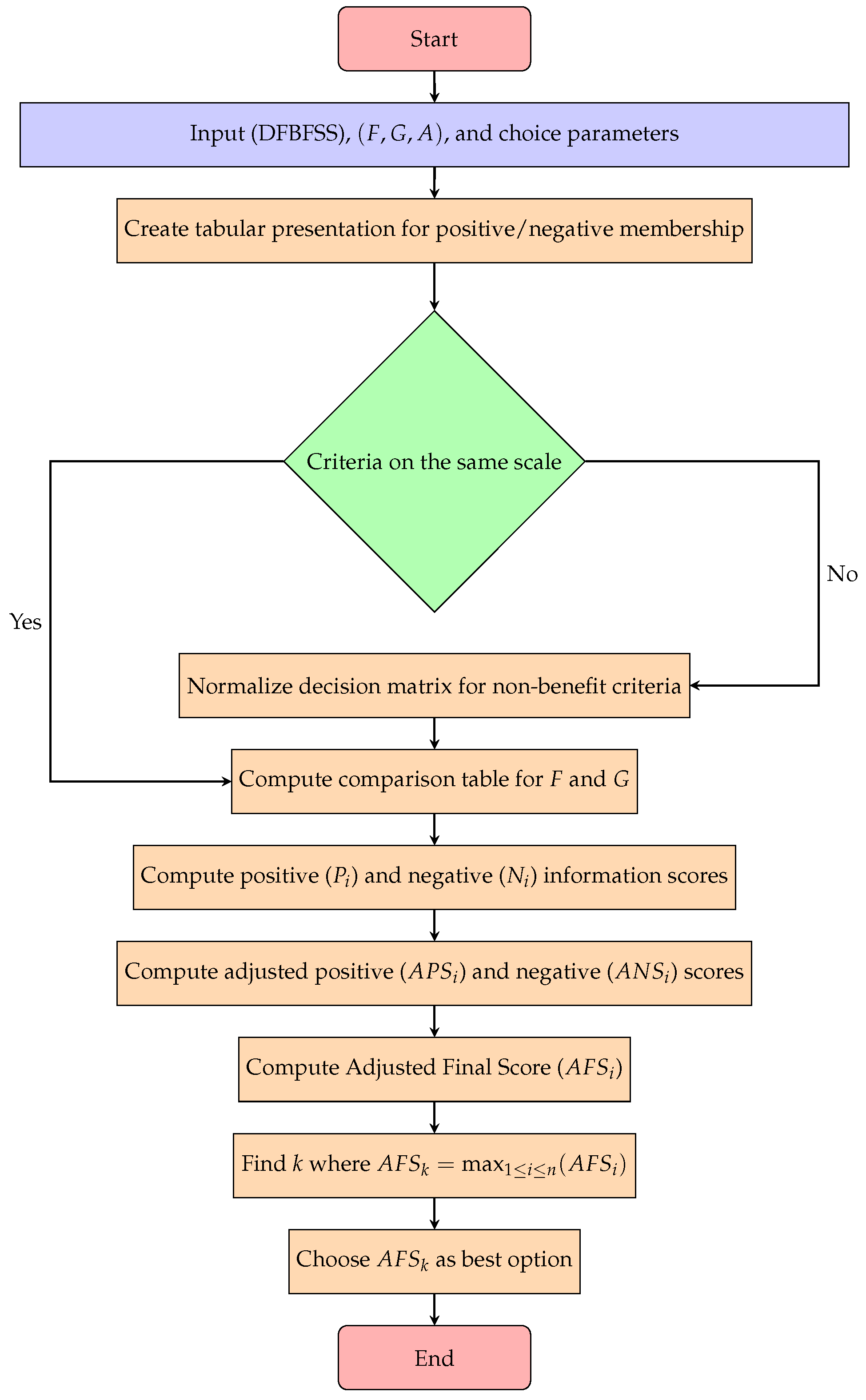
Algorithm. The algorithm and stepwise procedure of DFBFSS for choosing the best option is provided as:

Step 1:

The algorithm begins by accepting a Double-Frame Bipolar Fuzzy Soft Set (DFBFSS) $(\vartheta ,\xi ,\Gamma )$, where $\left(\vartheta \right)$ is the set of alternatives, $\left(\xi \right)$ the set of criteria, and $\left(\Gamma \right)$ the mapping that assigns to each alternative-criterion pair a tuple of four membership values: positive membership ${\varrho }^{+}$, its negation ${\eta }^{+}$, negative membership ${\varrho }^{-}$, and its negation ${\eta }^{-}$. These values, derived from expert judgment or data, are then systematically organized into a decision matrix (tabular form), with rows representing alternatives, columns representing criteria, and each cell containing the corresponding four-dimensional membership tuple. This matrix serves as the structured input, clearly presenting both supporting and opposing evaluations alongside their respective negations for all considered factors.

Step 2:

Normalizing is required if the criteria are not on the same scale. This involves normalizing the decision matrix based on the characteristics of each criterion by using the Definition 11, i.e., for each non-benefit criterion, the normalization operation applies the complement definition to each membership component—for example, transforming the original positive membership ${\varrho }^{+}$ into $1-{\varrho }^{+}$ or a structurally equivalent complement, ensuring all criteria contribute uniformly within the bipolar fuzzy framework while preserving the relational logic between a membership and its negation. Benefit criteria remain unchanged, as their original values are already aligned with the desired direction of preference.

Step 3:

In this step, comparison tabular for functions F and G is computed using Definition 20. The following three steps are found using Definition 21.

Step 4:

Positive $\left(P_i\right)$ and negative $\left(N_i\right)$ information scores with their negations $(\neg P_i)$ and $(\neg N_i)$ are computed.

Step 5:

Adjusted positive $\left(AP{S}_i\right)$ and negative $\left(AN{S}_i\right)$ information scores with their negations are computed.

Step 6:

Adjusted Final score $\left(AF{S}_i\right)$ is computed.

Step 7:

Find k where $AF{S}_k={max}_{1\le i\le n}AF{S}_i$.

Step 8:

For $k=1,2,\dots ,n$, $AF{S}_k$ is the best choice to be chosen.

The overall structure of the proposed decision-making algorithm is illustrated in Figure 2.

The illustrative example used in this study is intentionally simplified to clearly demonstrate the operational mechanism of the proposed DFBFSS framework. Such synthetic examples are standard in the development of new fuzzy set models, where the primary objective is to validate structural behavior and decision consistency before large-scale empirical deployment.

The following section declares a numerical example on the above algorithm in order to verify the feasibility of the proposed method procedure.

6. Numerical Example

A family is searching for a residential apartment and assess their options based on some criteria. Let $\Lambda =\{{\varsigma }_1,{\varsigma }_2,{\varsigma }_3,{\varsigma }_4,{\varsigma }_5,{\varsigma }_6\}$ be a set of six apartments. Consider ${\rm Y}=\{{\rho }_1=$ affordability monthly rent, ${\rho }_2=$ accessibility to public transport, ${\rho }_3=$ schools proximity and ${\rho }_4=$ noise levels} be a set of parameters. Also, let the negation set of ${\rm Y}$ be $\neg {\rm Y}=\{\neg {\rho }_1=$ unaffordability monthly rent, $\neg {\rho }_2=$ no public transport, $\neg {\rho }_3=$ school remoteness and $\neg {\rho }_4=$ quietness levels}. Following a thorough discussion, the family members determine that each apartment will be evaluated using a favorable subset $\Gamma =\{{\rho }_1,{\rho }_3,{\rho }_4\}$ of ${\rm Y}$.

Step 1: Input $\left(DFBFSS\right)$ $(\vartheta ,\xi ,\Gamma )$ (see

Table 11. Table of $(\vartheta ,\xi ,\Gamma )$.

	$\mathbf{(}\mathit{\vartheta }\mathbf{,}\mathit{\Gamma }\mathbf{)}$			$\mathbf{(}\mathit{\xi }\mathbf{,}\mathbf{\neg }\mathit{\Gamma }\mathbf{)}$
	$\mathsf{\vartheta }\mathbf{\left(}{\mathsf{\rho }}_{\mathbf{1}}\mathbf{\right)}$	$\mathsf{\vartheta }\mathbf{\left(}{\mathsf{\rho }}_{\mathbf{3}}\mathbf{\right)}$	$\mathsf{\vartheta }\mathbf{\left(}{\mathsf{\rho }}_{\mathbf{4}}\mathbf{\right)}$	$\mathsf{\xi }\mathbf{(}\mathbf{\neg }{\mathsf{\rho }}_{\mathbf{1}}\mathbf{)}$	$\mathsf{\xi }\mathbf{(}\mathbf{\neg }{\mathsf{\rho }}_{\mathbf{3}}\mathbf{)}$	$\mathsf{\xi }\mathbf{\left(}{\mathsf{\rho }}_{\mathbf{4}}\mathbf{\right)}$
${\varsigma }_1$	$(0.35,-0.3)$	$(0.4,-0.25)$	$(0.5,-0.7)$	$(0.1,-0.4)$	$(0.6,-0.5)$	$(0.3,-0.23)$
${\varsigma }_2$	$(0.45,-0.2)$	$(0.65,-0.4)$	$(0.3,-0.8)$	$(0.37,-0.4)$	$(0.22,-0.6)$	$(0.64,-0.1)$
${\varsigma }_3$	$(0.45,-0.43)$	$(0.2,-0.7)$	$(0.8,-0.6)$	$(0.4,-0.15)$	$(0.5,-0.2)$	$(0.2,-0.3)$
${\varsigma }_4$	$(0.7,-0.5)$	$(0.8,-0.6)$	$(0.74,-0.31)$	$(0.25,-0.3)$	$(0.1,-0.4)$	$(0.1,-0.49)$
${\varsigma }_5$	$(0.74,-0.6)$	$(0.39,-0.7)$	$(0.7,-0.8)$	$(0.2,-0.4)$	$(0.5,-0.25)$	$(0.2,-0.1)$
${\varsigma }_6$	$(0.46,-0.1)$	$(0.6,-0.6)$	$(0.33,-0.8)$	$(0.1,-0.31)$	$(0.1,-0.3)$	$(0.52,-0.1)$

) and choice parameters for family (see

Table 12. Tabular presentation for ${\varrho }^{+}.$

$\mathit{\vartheta }$	${\mathit{\rho }}_1$	${\mathit{\rho }}_3$	${\mathit{\rho }}_{\mathbf{4}}$
${\varsigma }_1$	$0.35$	$0.4$	$0.5$
${\varsigma }_2$	$0.45$	$0.65$	$0.3$
${\varsigma }_3$	$0.45$	$0.2$	$0.8$
${\varsigma }_4$	$0.7$	$0.8$	$0.74$
${\varsigma }_5$	$0.74$	$0.39$	$0.7$
${\varsigma }_6$	$0.46$	$0.6$	$0.33$

,

Table 13. Tabular presentation for ${\neg \eta }^{+}$.

$\mathit{\xi }$	$\mathbf{\neg }{\mathit{\rho }}_{\mathbf{1}}$	$\mathbf{\neg }{\mathit{\rho }}_{\mathbf{3}}$	$\mathbf{\neg }{\mathit{\rho }}_{\mathbf{4}}$
${\varsigma }_1$	$0.1$	$0.6$	$0.3$
${\varsigma }_2$	$0.37$	$0.22$	$0.65$
${\varsigma }_3$	$0.4$	$0.5$	$0.2$
${\varsigma }_4$	$0.25$	$0.1$	$0.1$
${\varsigma }_5$	$0.2$	$0.5$	$0.2$
${\varsigma }_6$	$0.1$	$0.1$	$0.52$

,

Table 14. Tabular presentation for ${\varrho }^{-}$.

$\mathit{\vartheta }$	${\mathit{\rho }}_{\mathbf{1}}$	${\mathit{\rho }}_{\mathbf{3}}$	${\mathit{\rho }}_{\mathbf{4}}$
${\varsigma }_1$	$-0.3$	$-0.25$	$-0.7$
${\varsigma }_2$	$-0.2$	$-0.4$	$-0.8$
${\varsigma }_3$	$-0.43$	$-0.7$	$-0.6$
${\varsigma }_4$	$-0.5$	$-0.6$	$-0.31$
${\varsigma }_5$	$-0.6$	$-0.7$	$-0.8$
${\varsigma }_6$	$-0.1$	$-0.6$	$-0.8$

and

Table 15. Tabular presentation for ${\neg \eta }^{-}.$

$\mathit{\xi }$	$\mathbf{\neg }{\mathit{\rho }}_{\mathbf{1}}$	$\mathbf{\neg }{\mathit{\rho }}_{\mathbf{3}}$	$\mathbf{\neg }{\mathit{\rho }}_{\mathbf{4}}$
${\varsigma }_1$	$-0.4$	$-0.5$	$-0.23$
${\varsigma }_2$	$-0.4$	$-0.6$	$-0.1$
${\varsigma }_3$	$-0.15$	$-0.2$	$-0.3$
${\varsigma }_4$	$-0.3$	$-0.4$	$-0.49$
${\varsigma }_5$	$-0.4$	$-0.25$	$-0.1$
${\varsigma }_6$	$-0.31$	$-0.3$	$-0.1$

).

Step 2: Normalization is needed in this step as the criteria are not in the same scale (see

Table 16. Normalized tabular presentation for ${\varrho }^{+}$.

$\mathit{\vartheta }$	${\mathit{\rho }}_{\mathbf{1}}$	${\mathit{\rho }}_{\mathbf{3}}$	${\mathit{\rho }}_{\mathbf{4}}$
${\varsigma }_1$	$0.35$	$0.6$	$0.5$
${\varsigma }_2$	$0.45$	$0.35$	$0.7$
${\varsigma }_3$	$0.45$	$0.8$	$0.2$
${\varsigma }_4$	$0.7$	$0.2$	$0.26$
${\varsigma }_5$	$0.74$	$0.61$	$0.3$
${\varsigma }_6$	$0.46$	$0.4$	$0.67$

,

Table 17. Normalized tabular presentation for ${\neg \eta }^{+}$.

$\mathit{\xi }$	$\mathbf{\neg }{\mathit{\rho }}_{\mathbf{1}}$	$\mathbf{\neg }{\mathit{\rho }}_{\mathbf{3}}$	$\mathbf{\neg }{\mathit{\rho }}_{\mathbf{4}}$
${\varsigma }_1$	$0.9$	$0.6$	$0.3$
${\varsigma }_2$	$0.63$	$0.22$	$0.65$
${\varsigma }_3$	$0.6$	$0.5$	$0.2$
${\varsigma }_4$	$0.75$	$0.1$	$0.1$
${\varsigma }_5$	$0.8$	$0.5$	$0.2$
${\varsigma }_6$	$0.9$	$0.1$	$0.52$

,

Table 18. Normalized tabular presentation for ${\varrho }^{-}$.

$\mathit{\vartheta }$	${\mathit{\rho }}_{\mathbf{1}}$	${\mathit{\rho }}_{\mathbf{3}}$	${\mathit{\rho }}_{\mathbf{4}}$
${\varsigma }_1$	$-0.3$	$-0.75$	$-0.3$
${\varsigma }_2$	$-0.2$	$-0.6$	$-0.2$
${\varsigma }_3$	$-0.43$	$-0.3$	$-0.4$
${\varsigma }_4$	$-0.5$	$-0.4$	$-0.69$
${\varsigma }_5$	$-0.6$	$-0.3$	$-0.2$
${\varsigma }_6$	$-0.1$	$-0.4$	$-0.2$

and

Table 19. Normalized tabular presentation for ${\neg \eta }^{-}$.

$\mathit{\xi }$	$\mathbf{\neg }{\mathit{\rho }}_{\mathbf{1}}$	$\mathbf{\neg }{\mathit{\rho }}_{\mathbf{3}}$	$\mathbf{\neg }{\mathit{\rho }}_{\mathbf{4}}$
${\varsigma }_1$	$-0.6$	$-0.5$	$-0.23$
${\varsigma }_2$	$-0.6$	$-0.6$	$-0.1$
${\varsigma }_3$	$-0.85$	$-0.2$	$-0.3$
${\varsigma }_4$	$-0.7$	$-0.4$	$-0.49$
${\varsigma }_5$	$-0.6$	$-0.25$	$-0.1$
${\varsigma }_6$	$-0.69$	$-0.3$	$-0.1$

).

Step 3: In this step, comparison tabular for ${\varrho }^{+}$, ${\varrho }^{-}$ with their negations ${\neg \eta }^{+}$ and ${\neg \eta }^{-}$, respectively, is used (see

Table 20. Comparison of normalized tabular presentation for ${\varrho }^{+}.$

	${\mathit{\varsigma }}_{\mathbf{1}}$	${\mathit{\varsigma }}_{\mathbf{2}}$	${\mathit{\varsigma }}_{\mathbf{3}}$	${\mathit{\varsigma }}_{\mathbf{4}}$	${\mathit{\varsigma }}_{\mathbf{5}}$	${\mathit{\varsigma }}_{\mathbf{6}}$
${\varsigma }_1$	3	1	1	2	1	1
${\varsigma }_2$	2	3	2	2	1	1
${\varsigma }_3$	2	2	3	1	1	1
${\varsigma }_4$	1	1	2	3	0	1
${\varsigma }_5$	2	2	2	3	3	2
${\varsigma }_6$	2	1	2	2	1	3

,

Table 21. Comparison of normalized tabular presentation for ${\neg \eta }^{+}.$

	${\mathit{\varsigma }}_{\mathbf{1}}$	${\mathit{\varsigma }}_{\mathbf{2}}$	${\mathit{\varsigma }}_{\mathbf{3}}$	${\mathit{\varsigma }}_{\mathbf{4}}$	${\mathit{\varsigma }}_{\mathbf{5}}$	${\mathit{\varsigma }}_{\mathbf{6}}$
${\varsigma }_1$	3	1	0	0	0	2
${\varsigma }_2$	2	3	1	1	2	1
${\varsigma }_3$	3	2	3	1	3	2
${\varsigma }_4$	3	2	2	3	3	3
${\varsigma }_5$	3	1	2	0	3	2
${\varsigma }_6$	2	2	1	1	1	3

,

Table 22. Comparison of normalized tabular presentation for ${\varrho }^{-}$.

	${\mathit{\varsigma }}_{\mathbf{1}}$	${\mathit{\varsigma }}_{\mathbf{2}}$	${\mathit{\varsigma }}_{\mathbf{3}}$	${\mathit{\varsigma }}_{\mathbf{4}}$	${\mathit{\varsigma }}_{\mathbf{5}}$	${\mathit{\varsigma }}_{\mathbf{6}}$
${\varsigma }_1$	3	3	1	1	2	3
${\varsigma }_2$	0	3	1	1	2	3
${\varsigma }_3$	2	2	3	0	2	2
${\varsigma }_4$	2	2	3	3	2	3
${\varsigma }_5$	1	2	2	1	3	2
${\varsigma }_6$	0	1	1	1	2	3

and

Table 23. Comparison of normalized tabular presentation for ${\neg \eta }^{-}$.

	${\mathit{\varsigma }}_{\mathbf{1}}$	${\mathit{\varsigma }}_{\mathbf{2}}$	${\mathit{\varsigma }}_{\mathbf{3}}$	${\mathit{\varsigma }}_{\mathbf{4}}$	${\mathit{\varsigma }}_{\mathbf{5}}$	${\mathit{\varsigma }}_{\mathbf{6}}$
${\varsigma }_1$	3	2	2	2	1	1
${\varsigma }_2$	2	3	2	2	2	2
${\varsigma }_3$	1	1	3	2	1	1
${\varsigma }_4$	1	1	1	3	0	0
${\varsigma }_5$	3	3	2	3	3	3
${\varsigma }_6$	2	2	2	3	1	3

).

Step 4: Positive and negative information scores with their negations are computed in this step (see

Table 24. Normalized tabular presentation score for ${\varrho }^{+}$.

	Row Sum: ${\mathit{r}}_{\mathit{i}}$	Column Sum: ${\mathit{c}}_{\mathit{i}}$	${\mathit{P}}_{\mathit{i}}={\mathit{r}}_{\mathit{i}}\mathbf{-}{\mathit{c}}_{\mathit{i}}$
${\varsigma }_1$	9	12	$-3$
${\varsigma }_2$	11	10	$1$
${\varsigma }_3$	10	12	$-2$
${\varsigma }_4$	8	13	$-5$
${\varsigma }_5$	14	7	$7$
${\varsigma }_6$	11	9	$2$

,

Table 25. Normalized tabular presentation score for ${\neg \eta }^{+}$.

	Row Sum: $\mathbf{\neg }{\mathit{r}}_{\mathit{i}}$	Column Sum: $\mathbf{\neg }{\mathit{\hslash }}_{\mathit{i}}$	$\mathbf{\neg }{\mathit{P}}_{\mathit{i}}\mathbf{=}\mathbf{\neg }{\mathit{r}}_{\mathit{i}}\mathbf{-}\mathbf{\neg }{\mathit{\hslash }}_{\mathit{i}}$
${\varsigma }_1$	6	16	$-10$
${\varsigma }_2$	10	11	$-1$
${\varsigma }_3$	14	9	$5$
${\varsigma }_4$	16	6	$10$
${\varsigma }_5$	11	12	$-1$
${\varsigma }_6$	10	13	$-3$

,

Table 26. Normalized tabular presentation score for ${\varrho }^{-}$.

	Row Sum: ${\mathit{r}}_{\mathit{i}}^{\mathbf{\prime }}$	Column Sum: ${\mathit{c}}_{\mathit{i}}^{\mathbf{\prime }}$	${\mathit{N}}_{\mathit{i}}\mathbf{=}{{\mathit{r}}^{\mathbf{\prime }}}_{\mathit{i}}\mathbf{-}{{\mathit{c}}^{\mathbf{\prime }}}_{\mathit{i}}$
${\varsigma }_1$	13	8	$5$
${\varsigma }_2$	10	13	$-3$
${\varsigma }_3$	11	11	$0$
${\varsigma }_4$	15	7	$8$
${\varsigma }_5$	11	13	$-2$
${\varsigma }_6$	8	16	$-8$

and

Table 27. Normalized tabular presentation score for ${\neg \eta }^{-}$.

	Row Sum: $\mathbf{\neg }\mathbf{\prime }{\mathit{r}}_{\mathit{i}}$	Column Sum: $\mathbf{\neg }{\mathit{\hslash }}_{\mathit{i}}^{\mathbf{\prime }}$	$\mathbf{\neg }{\mathit{N}}_{\mathit{i}}\mathbf{=}\mathbf{\neg }{{\mathit{r}}^{\mathbf{\prime }}}_{\mathit{i}}\mathbf{-}\mathbf{\neg }{{\mathit{c}}^{\mathbf{\prime }}}_{\mathit{i}}$
${\varsigma }_1$	11	12	$-2$
${\varsigma }_2$	13	12	$1$
${\varsigma }_3$	9	12	$-3$
${\varsigma }_4$	6	15	$-9$
${\varsigma }_5$	17	8	$9$
${\varsigma }_6$	13	10	$3$

).

Step 5: Adjusted positive and negative information scores with their negations are computed in this step (see

Table 28. Adjusted Positive score(APS).

	${\mathit{P}}_{\mathit{i}}$	$\mathbf{\neg }{\mathit{P}}_{\mathit{i}}$	${\mathit{APS}}_{\mathit{i}}\mathbf{=}{\mathit{P}}_{\mathit{i}}\mathbf{-}\mathbf{(}\mathbf{\neg }{\mathit{P}}_{\mathit{i}}\mathbf{)}$
${\varsigma }_1$	$-3$	$-10$	$7$
${\varsigma }_2$	$1$	$-1$	$2$
${\varsigma }_3$	$-2$	$5$	$-7$
${\varsigma }_4$	$-5$	$10$	$-15$
${\varsigma }_5$	$7$	$-1$	$8$
${\varsigma }_6$	$2$	$-3$	$5$

and

Table 29. Adjusted negative score(ANS).

	${\mathit{N}}_{\mathit{i}}$	$\mathbf{\neg }{\mathit{N}}_{\mathit{i}}$	${\mathit{ANS}}_{\mathit{i}}\mathbf{=}{\mathit{N}}_{\mathit{i}}\mathbf{-}\mathbf{(}\mathbf{\neg }{\mathit{N}}_{\mathit{i}}\mathbf{)}$
${\varsigma }_1$	$5$	$-2$	$7$
${\varsigma }_2$	$-3$	$1$	$-4$
${\varsigma }_3$	$0$	$-3$	$3$
${\varsigma }_4$	$8$	$-9$	$17$
${\varsigma }_5$	$-2$	$9$	$-11$
${\varsigma }_6$	$-8$	$3$	$-11$

).

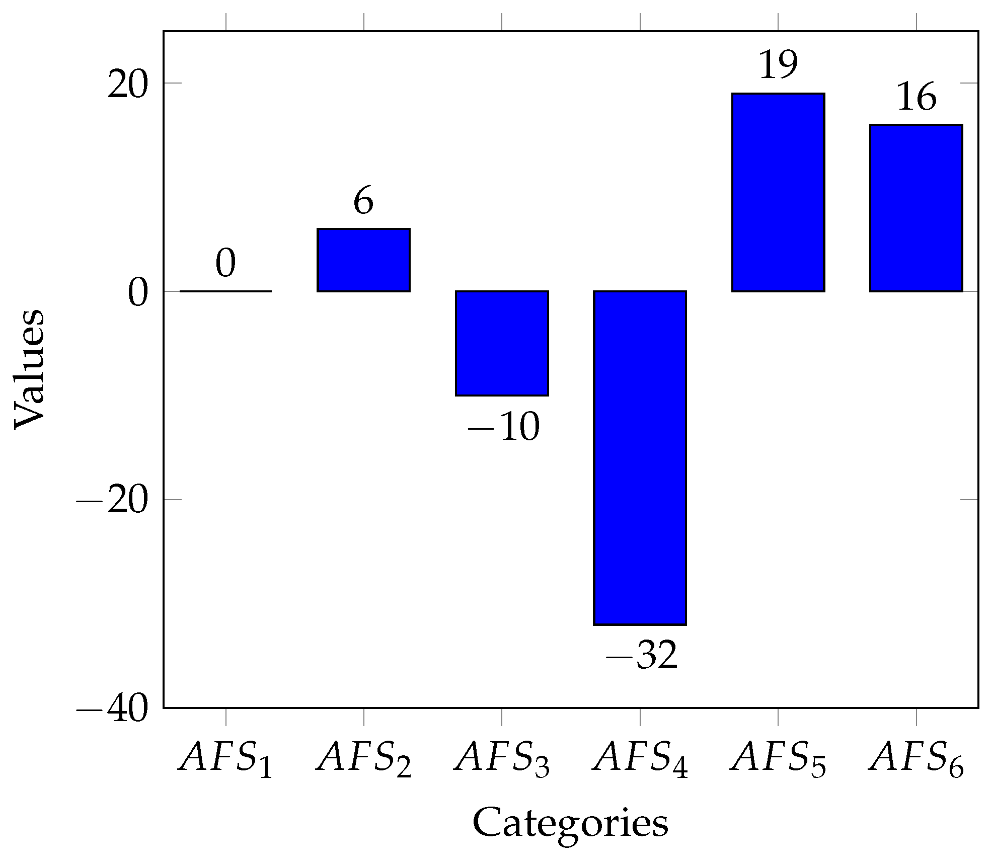
Step 6: Table for adjusted final score (AFS): (See Figure 3)

Step 7: From

Table 30. Adjusted final score (AFS).

	${\mathit{APS}}_{\mathit{i}}$	${\mathit{ANS}}_{\mathit{i}}$	${\mathit{AFS}}_{\mathit{i}}\mathbf{=}{\mathit{APS}}_{\mathit{i}}\mathbf{-}{\mathit{ANS}}_{\mathit{i}}$
${\varsigma }_1$	$7$	$7$	$0$
${\varsigma }_2$	$2$	$-4$	$6$
${\varsigma }_3$	$-7$	$3$	$-10$
${\varsigma }_4$	$-15$	$17$	$-32$
${\varsigma }_5$	$8$	$-11$	$19$
${\varsigma }_6$	$5$	$-11$	$16$

, fifth apartment $AF{S}_5$ is chosen to the best one among all.

7. Comparative Analysis

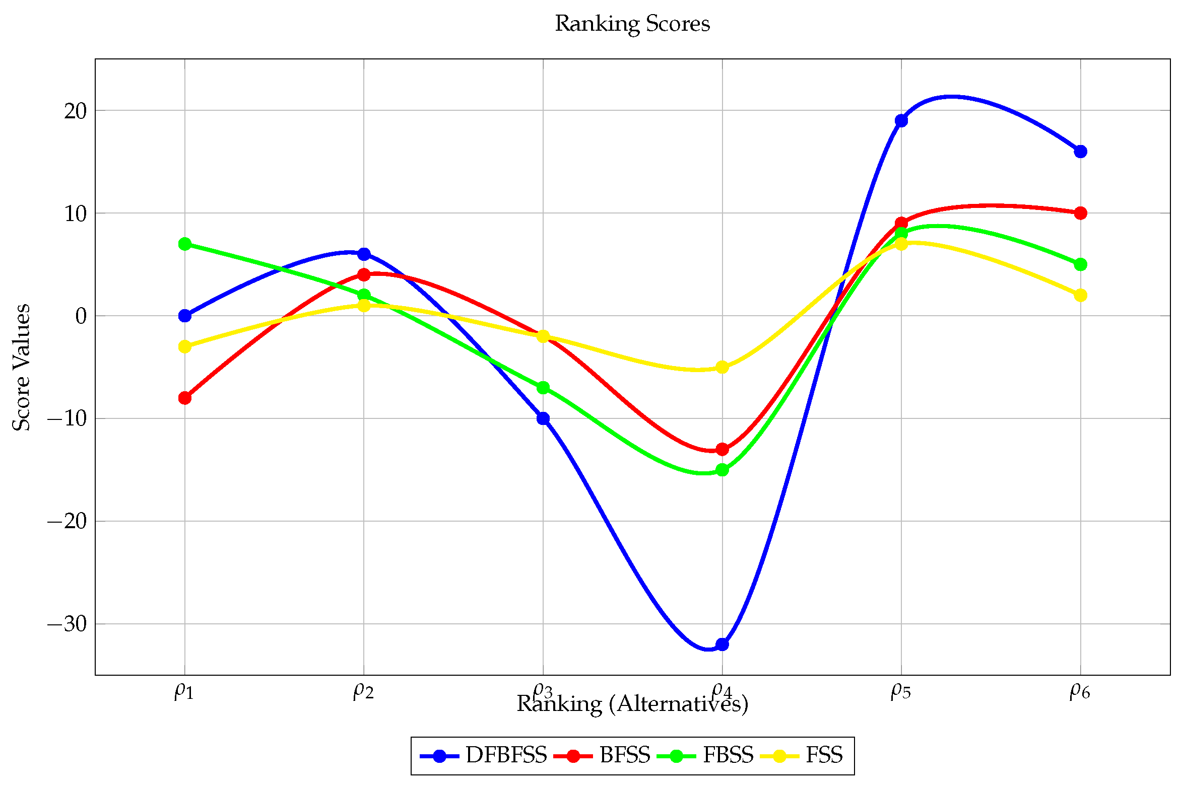
The DFBFSS seems to be an enhancement and an interconnection between bipolar fuzzy sets BFS and bipolar soft sets BSS, which serve as foundations for the proposed method. In this section, the suggested set is compared with certain existing ones in order to further confirm the correctness of the suggested approaches such as bipolar fuzzy soft set (BFSS) [34], fuzzy bipolar soft set (FBSS) [40] and fuzzy soft set (FSS) [27]. The details are demonstrated in

Table 31. Comparative analysis of DFBFSS with some existing sets.

Models	Ranking Results	Optimal Alternative
DFBFSS	${\varsigma }_5\succ {\varsigma }_6\succ {\varsigma }_2\succ {\varsigma }_1\succ {\varsigma }_3\succ {\varsigma }_4$	${\varsigma }_5$
FSS	${\varsigma }_5\succ {\varsigma }_6\succ {\varsigma }_2\succ {\varsigma }_3\succ {\varsigma }_1\succ {\varsigma }_4$	${\varsigma }_5$
FBSS	${\varsigma }_5\succ {\varsigma }_1\succ {\varsigma }_6\succ {\varsigma }_2\succ {\varsigma }_3\succ {\varsigma }_4$	${\varsigma }_5$
BFSS	${\varsigma }_6\succ {\varsigma }_5\succ {\varsigma }_2\succ {\varsigma }_3\succ {\varsigma }_1\succ {\varsigma }_4$	${\varsigma }_6$

and Figure 4.

Unlike SS, FSS, and BFSS models, the proposed DFBFSS framework explicitly distinguishes between membership, counter-membership, and their negations, enabling symmetric handling of conflicting information.

The following comparative analysis in

Table 32. Comparative Analysis of the Proposed DFBFSS Model with Related.

Aspect/Model	Soft Set (SS)	Fuzzy Soft Set (FSS)	Bipolar FSS (BFSS)	Proposed DFBFSS
Handles Vague Data	No (Crisp)	Yes	Yes	Yes
Models Bipolarity	No	No	Yes	Yes
Captures Negation	No	No	No	Yes
Complexity of Representation	Low	Medium	Medium	High (Four-dimensional)
Key Justification	Oversimplifies due to crisp logic	Misses conflicting criteria	Misses negation semantics	Captures complete expert judgment with dual-frame uncertainty

elucidates the theoretical and practical advancements of the DFBFSS framework by benchmarking it against its direct predecessors, clearly demonstrating how its unique capacity to model four-dimensional judgment leads to more nuanced and robust decision outcomes.

Table 32 provides a direct comparison between the proposed DFBFSS-based decision-making method and existing models such as SS, FSS, and BFSS. Unlike these approaches, which rely on single- or two-dimensional evaluations, the DFBFSS framework incorporates four complementary evaluative components: positive membership, negative membership, and their respective negations. This enriched structure allows the proposed method to preserve conflicting and incomplete information that is either ignored or collapsed in traditional models. As a result, the final ranking produced by the DFBFSS method reflects a more balanced and informative aggregation of expert opinions. This demonstrates that the advantage of the proposed approach lies not in numerical dominance but in its superior expressive power and its ability to model dual and contradictory assessments within a unified decision-making framework.

To clarify the distinctive features of the proposed DFBFSS framework and its advantages over existing models, a comparative analysis is summarized in

Table 33. Comparison of DFBFSSs with Existing Fuzzy Soft Models.

Model	Positive Membership	Negative Membership	Negation	Bipolarity	Multi-Criteria Decision Support	Notes
SS [23]	✓	×	×	×	Limited	Binary or crisp values only
FSS [27]	✓	×	×	×	Moderate	Captures positive fuzziness only
BFSS [34]	✓	✓	×	✓	Moderate	No negation information
DFBFSS (Proposed)	✓	✓	✓	✓	High	Four-dimensional, dual-frame, handles negation

.

Table 33 clearly demonstrates that the proposed DFBFSS framework uniquely integrates bipolarity, negation semantics, and a dual-frame structure, which collectively enhance its suitability for complex multi-criteria decision-making problems.

8. Conclusions

The bipolar fuzzy set and bipolar soft set have evolved into robust frameworks, paving the way for the development of the theory of double-framed bipolar fuzzy soft sets (DFBFSSs). This innovative model provides a dual-layered structure for representing elements through ordered pairs of positive and negative membership grades, offering a nuanced perspective on uncertainty. Fundamental operations like subset relationships, equality, complement, intersection, and union have been rigorously defined and illustrated with numerical examples, demonstrating the practicality and applicability of DFBFSSs in complex decision-making and information modeling scenarios. In order to confirm the applicability of the suggested model, a numerical example has been provided along with an application of double-framed bipolar fuzzy soft sets to a decision-making problem and a general method to solve it. A comparison between the proposed strategy and some other existing ones has been given in order to verify the feasibility of the proposed decision-making process. This work establishes a formally symmetric extension of bipolar fuzzy soft set theory, introducing a nontrivial automorphism-invariant structure that is not captured by existing fuzzy or bipolar models.

Importantly, the symmetric structure of DFBFSSs preserves the inherent balance between positive and negative information, further enhancing their applicability in complex decision-making scenarios.

Future work will focus on both theoretical and practical extensions of the proposed framework. From a theoretical perspective, the DFBFSS model may be extended to more advanced settings such as intuitionistic, Pythagorean, and q-rung orthopair structures, as well as further investigations into its topological and functional properties. From a practical perspective, future studies will apply the DFBFSS framework to real-world datasets, including medical diagnosis and supplier selection problems, and will compare its performance with BFSS- and FSS-based decision-making models using expert-derived data and established evaluation criteria.

References

1. Ali, G.; Akram, M.; Koam, A.N.; Alcantud, J.C.R. Parameter reductions of bipolar fuzzy soft sets with their decision-making algorithms. Symmetry 2019, 11, 949. [Google Scholar] [CrossRef]
2. Zadeh, L.A. Fuzzy sets. Inf. Control 1965, 8, 338–353. [Google Scholar] [CrossRef]
3. Bellman, R.E.; Zadeh, L.A. Decision-making in a fuzzy environment. Manag. Sci. 1970, 17, B-141–B-164. [Google Scholar] [CrossRef]
4. Dubois, D. The role of fuzzy sets in decision sciences: Old techniques and new directions. Fuzzy Sets Syst. 2011, 184, 3–28. [Google Scholar] [CrossRef]
5. Tong, R.M. Fuzzy control systems: A retrospective. In Proceedings of the 1983 American Control Conference, San Francisco, CA, USA, 22–24 June 1983; pp. 1224–1229. [Google Scholar]
6. Bezdek, J.C. Pattern Recognition with Fuzzy Objective Function Algorithms; Springer Science & Business Media: Berlin/Heidelberg, Germany, 2013. [Google Scholar]
7. Pedrycz, W. Fuzzy sets in pattern recognition: Methodology and methods. Pattern Recognit. 1990, 23, 121–146. [Google Scholar] [CrossRef]
8. Kandel, A.; Schneider, M. Fuzzy sets and their applications to artificial intelligence. Adv. Comput. 1989, 28, 69–105. [Google Scholar]
9. Kahraman, C.; Onar, S.C.; Oztaysi, B.; Cebi, S. Role of Fuzzy Sets on Artificial Intelligence Methods: A literature. Trans. Fuzzy Sets Syst. 2023, 2, 158–178. [Google Scholar]
10. Chen, C.-T.; Lin, C.-T.; Huang, S.-F. A fuzzy approach for supplier evaluation and selection in supply chain management. Int. J. Prod. Econ. 2006, 102, 289–301. [Google Scholar] [CrossRef]
11. Taherdoost, H.; Madanchian, M. Decision making: Models, processes, techniques. Cloud Comput. Data Sci. 2024, 5, 1–14. [Google Scholar] [CrossRef]
12. Litvaj, I.; Ponisciakova, O.; Stancekova, D.; Svobodova, J.; Mrazik, J. Decision-making procedures and their relation to knowledge management and quality management. Sustainability 2022, 14, 572. [Google Scholar] [CrossRef]
13. Mu, E. Multicriteria decision making as interdisciplinary research. Int. J. Anal. Hierarchy Process. 2022, 14. [Google Scholar] [CrossRef]
14. Newell, W.H. Decision Making in Interdisciplinary Studies. In Handbook of Decision Making; Morçöl, G., Ed.; CRC Press/Taylor & Francis Group: New York, NY, USA, 2007; pp. 245–264. [Google Scholar]
15. Schmude, T.; Koesten, L.; Möller, T.; Tschiatschek, S. Applying Interdisciplinary Frameworks to Understand Algorithmic Decision-Making. arXiv 2023, arXiv:2305.16700. [Google Scholar]
16. Abubakar, A.M.; Elrehail, H.; Alatailat, M.A.; Elçi, A. Knowledge management, decision-making style and organizational performance. J. Innov. Knowl. 2019, 4, 104–114. [Google Scholar] [CrossRef]
17. AlDhaena, E. The role of knowledge management in strategic decision-making in higher education institutions (HEIs): A proposed model. Int. J. Innov. Creat. Change 2020, 10, 50–57. [Google Scholar]
18. Bruch, E.; Feinberg, F. Decision-making processes in social contexts. Annu. Rev. Sociol. 2017, 43, 207–227. [Google Scholar] [CrossRef]
19. Sayama, H.; Dionne, S.D. Studying collective human decision making and creativity with evolutionary computation. Artif. Life 2015, 21, 379–393. [Google Scholar] [CrossRef][Green Version]
20. Zafar, F.; Akram, M. A novel decision-making method based on rough fuzzy information. Int. J. Fuzzy Syst. 2018, 20, 1000–1014. [Google Scholar] [CrossRef]
21. Naz, S.; Ashraf, S.; Akram, M. A novel approach to decision-making with Pythagorean fuzzy information. Mathematics 2018, 6, 95. [Google Scholar] [CrossRef]
22. Zhang, W.R. bipolar fuzzy sets. In Proceedings of the 1998 IEEE International Conference on Fuzzy Systems Proceedings, IEEE World Congress on Computational Intelligence (Cat. No. 98CH36228), Anchorage, AK, USA, 4–9 May 1998; Volume 1, pp. 835–840. [Google Scholar]
23. Molodtsov, D. Soft set theory—First results. Comput. Math. Appl. 1999, 37, 19–31. [Google Scholar] [CrossRef]
24. Ali, M.I.; Shabir, M. Comments on De Morgan’s law in fuzzy soft sets. J. Fuzzy Math. 2010, 18, 679–686. [Google Scholar]
25. Ali, M.I. Another view on reduction of parameters in soft sets. Appl. Soft Comput. 2012, 12, 1814–1821. [Google Scholar] [CrossRef]
26. Feng, F.; Li, C.; Davvaz, B.; Ali, M.I. Soft sets combined with fuzzy sets and rough sets: A tentative approach. Soft Comput. 2010, 14, 899–911. [Google Scholar] [CrossRef]
27. Maji, P.K.R. Biswas ans AR Roy, “Fuzzy soft sets”. J. Fuzzy Math. 2001, 9, 589–602. [Google Scholar]
28. Roy, A.R.; Maji, P. A fuzzy soft set theoretic approach to decision making problems. J. Comput. Appl. Math. 2007, 203, 412–418. [Google Scholar] [CrossRef]
29. Pei, D.; Miao, D. A From soft sets to information systems. In Proceedings of the 2005 IEEE International Conference on Granular Computing, Beijing, China, 25–27 July 2005; Volume 2, pp. 617–621. [Google Scholar]
30. Yang, X.; Lin, T.Y.; Yang, J.; Li, Y.; Yu, D. Combination of interval-valued fuzzy set and soft set. Comput. Math. Appl. 2009, 58, 521–527. [Google Scholar] [CrossRef]
31. Shabir, M.; Naz, M. On bipolar soft sets. arXiv 2013, arXiv:1303.1344. [Google Scholar] [PubMed]
32. Mahmood, T. A novel approach towards bipolar soft sets and their applications. J. Math. 2020, 2020, 4690808. [Google Scholar] [CrossRef]
33. Lee, K.M. Bipolar-valued fuzzy sets and their operations. In Proceedings of the International Conference on Intelligent Technologies, Bangkok, Thailand, 12–14 December 2000; pp. 307–312. [Google Scholar]
34. Abdullah, S.; Aslam, M.; Ullah, K. Bipolar fuzzy soft sets and its applications in decision making problem. J. Intell. Fuzzy Syst. 2014, 27, 729–742. [Google Scholar] [CrossRef]
35. Musa, S.Y.; Asaad, B.A.; Alohali, H.; Ameen, Z.A.; Alqahtani, M.H. Fuzzy N-Bipolar Soft Sets for Multi-Criteria Decision-Making: Theory and Application. CMES-Comput. Model. Eng. Sci. 2025, 143, 911–943. [Google Scholar] [CrossRef]
36. Alqablan, K.A.; Alsager, K.M. Multi-Q Cubic bipolar fuzzy soft sets and cosine similarity methods for multi-criteria decision making. Symmetry 2025, 16, 1032. [Google Scholar] [CrossRef]
37. El-Atik, A.A.; Abu-Gdairi, R.; Nasef, A.A.; Jafari, S.; Badr, M. Fuzzy Soft Sets and Decision Making in Ideal Nutrition. Symmetry 2023, 15, 1523. [Google Scholar] [CrossRef]
38. Shi, D.; Khiamy, H.M.; Abbas, S.E.; Ibedou, I. Roughness of bipolar soft sets via ideals and its applications. Eur. J. Pure Appl. Math. 2025, 18, 6225. [Google Scholar] [CrossRef]
39. Maji, P.K.; Biswas, R.; Roy, A.R. Soft set theory. Comput. Math. Appl. 2003, 45, 555–562. [Google Scholar] [CrossRef]
40. Naz, M.; Shabir, M. On fuzzy bipolar soft sets, their algebraic structures and applications. J. Intell. Fuzzy Syst. 2014, 26, 1645–1656. [Google Scholar] [CrossRef]
Figure 1. From variant structures to fuzzy and soft sets to arriving at DFBFSSs.
Symmetry 18 00119 g001
Figure 2. Flowchart.
Symmetry 18 00119 g002
Figure 3. Adjusted final score.
Symmetry 18 00119 g003
Figure 4. Comparing DFBFSS with FSS, FBSS and BFSS.
Symmetry 18 00119 g004