Article

IAVOA–EATCN: An Adaptive Deep Framework for Accurate Power Load Forecasting

Faculty of Electrical and Control Engineering, Liaoning Technical University, Huludao 125000, China
*
Author to whom correspondence should be addressed.
Symmetry 2026, 18(1), 102; https://doi.org/10.3390/sym18010102
Submission received: 4 December 2025 / Revised: 24 December 2025 / Accepted: 3 January 2026 / Published: 6 January 2026
(This article belongs to the Section F: Engineering and Materials)

Abstract

With the large-scale integration of renewable energy, the operational complexity of power systems has increased, placing higher demands on the accuracy of load forecasting. To address the nonlinear characteristics of load variations and improve feature utilization, this paper proposes an IAVOA–EATCN load forecasting model. In the feature engineering stage, an expand–reduce transformation is employed to reconstruct the original multi-feature inputs, and variational mode decomposition (VMD) is further applied to extract low- and high-frequency components, thereby compressing redundant features while preserving essential information structures. In terms of model architecture, the nonlinear representation capability of the temporal convolutional network (TCN) is enhanced by introducing the FlexSwish activation function, and an Efficient Channel Attention (ECA) mechanism is integrated to strengthen the perception of critical features. For parameter optimization, an improved African Vulture Optimization Algorithm (IAVOA) is proposed, which initializes the population using perturbation-enhanced dynamic Tent mapping, balances global exploration and local exploitation through adaptive parameter control, and incorporates elite retention and migration mechanisms to avoid premature convergence. Experimental results on real-world load data demonstrate that the proposed model achieves RMSE, R2, and MAE values of 26.5544, 0.9804, and 18.5589, respectively, significantly outperforming benchmark methods and exhibiting strong generalization capability and practical potential for intelligent load forecasting.

1. Introduction

With the ongoing low-carbon and intelligent transformation of global energy systems, the operational characteristics of power systems are becoming increasingly nonlinear, non-stationary, and uncertain. As a key component of smart grid operation, scheduling, and planning, the accuracy of load forecasting directly affects both the economic efficiency of system operation and the integration level of renewable energy sources [1]. In the context of widespread distributed energy integration, the rapid development of electric mobility, and the continuous advancement of demand-side response, the multidimensional characteristics and dynamic patterns of load curves are becoming more complex. This evolution places higher demands on the temporal modeling capabilities and generalization performance of forecasting models [2]. Consequently, the development of highly accurate, robust, and interpretable load forecasting models has become a critical research focus in the field of intelligent power systems.
Traditional load forecasting approaches primarily rely on statistical modeling techniques, such as the Auto Regressive Integrated Moving Average (ARIMA) model and its seasonal variant (SARIMA), which perform well under conditions of stationary load sequences and strong periodic regularities [3]. However, in scenarios characterized by high volatility and strong randomness, such linear models struggle to capture the implicit relationships among nonlinear features. Machine learning methods, including Support Vector Machines (SVM) [4], Random Forests (RF) [5], and Extreme Gradient Boosting (XGBoost) [6], have made notable progress in feature modeling. Nevertheless, these approaches typically depend on manually constructed features and empirically tuned parameters, which limit their generalization capability and dynamic adaptability.
In contrast, deep learning techniques, with their end-to-end feature extraction and nonlinear representation capabilities, have demonstrated significant advantages in complex load forecasting tasks. Recurrent Neural Networks (RNNs) and their enhanced variant, Long Short-Term Memory networks (LSTM) [7], can effectively capture long-term dependencies in time series data. However, their recursive structure limits parallel computing efficiency and often leads to gradient vanishing issues when dealing with long sequences. To improve modeling efficiency and information transmission, Gated Recurrent Units (GRUs) were proposed to simplify the LSTM architecture, and have shown comparable or even superior performance in some tasks. Additionally, bidirectional structures such as BiLSTM [8] and BiGRU capture complete contextual dependencies by processing information in both forward and backward directions, thereby enhancing the model’s ability to represent global sequence features. Nevertheless, these recurrent models still face limitations in computational efficiency and modeling depth, making it difficult to balance training speed with the stability of long-term dependency modeling. On the other hand, Convolutional Neural Networks (CNNs) [9] possess the advantages of local feature extraction and parameter sharing, but their limited receptive field constrains their ability to model long-range temporal dependencies.
The Temporal Convolutional Network, which integrates dilated convolutions and residual connections, has demonstrated advantages in modeling long-term dependencies and enabling parallel computation. Its effectiveness has been validated in various tasks, including power load forecasting, wind power prediction, and demand response [10]. However, standard TCNs still face limitations in capturing nonlinear features, fusing multi-scale information, and optimizing model parameters [11]. To enhance its modeling capability, numerous improvements have been proposed. For instance, Han et al. introduced the Self-Attention TCN (SA-TCN), which incorporates multi-strategy optimization algorithms and self-attention mechanisms, significantly improving the modeling of complex temporal features [12]. Furthermore, Han et al. developed a hybrid framework combining CEEMDAN–SE–VMD signal decomposition with SA-TCN, which leverages multi-scale feature reconstruction and joint learning of high- and low-frequency components to improve forecasting accuracy under complex load patterns [13]. In parallel, Ma et al. proposed a BiStacking–TCN–GRU hybrid forecasting model, which utilizes a stacked ensemble learning strategy to combine the local feature extraction capability of TCN with the long-term dependency modeling strength of GRU. This approach effectively enhances the model’s generalization and stability [14]. Although these studies have made significant progress in structural design, feature representation, and model fusion, challenges remain in terms of adaptive parameter optimization, search efficiency, and the model’s responsiveness to sudden load fluctuations.
To address the aforementioned limitations, this paper proposes a systematic enhancement of the original TCN architecture, termed the Enhanced Adaptive Temporal Convolutional Network (EATCN). This model improves the nonlinear representation capability and temporal dependency extraction for complex load sequences by optimizing the activation function and channel-wise feature modeling mechanism. Specifically, a novel FlexSwish activation function is introduced, incorporating a tunable parameter to control the response on the negative axis and enable a smooth transition. This design allows the model to retain linear characteristics on the positive axis while enabling flexible responses on the negative side, effectively mitigating the “dead zone” issue associated with ReLU during gradient propagation. As a result, it significantly enhances training stability and representation continuity in deep networks. In addition, to strengthen the model’s adaptive recognition of critical features, a lightweight Efficient Channel Attention mechanism is embedded within the residual blocks of the TCN. This module facilitates channel-wise feature reweighting and local dependency modeling, thereby improving prediction accuracy and generalization performance without introducing significant computational overhead. In summary, the EATCN model is structurally better aligned with the temporal characteristics and physical constraints inherent in power load data.
To further enhance the overall performance and stability of the forecasting model, this paper proposes an Improved African Vulture Optimization Algorithm to automatically optimize the key hyperparameters of the model. Addressing the limitations of the original African Vulture Optimization Algorithm—including strong randomness in population initialization, low search efficiency, and poor convergence accuracy in later stages [15]—the proposed IAVOA maintains the original bio-inspired framework while introducing three improvements.
First, a Perturbation-enhanced Dynamic Tent Mapping (PDTM) is adopted to improve the uniformity of the initial population distribution. Second, an adaptive control parameter mechanism is employed to balance global exploration and local exploitation. Third, an elitism and migration strategy is integrated to prevent premature convergence. These enhancements significantly improve the search efficiency and stability of the algorithm without increasing computational complexity. When applied to the parameter tuning of the EATCN model, IAVOA demonstrates superior global optimization ability and generalization performance, providing reliable algorithmic support for complex load forecasting tasks.
Based on the above, the main contributions of this paper are summarized as follows: (1) An Enhanced Adaptive Temporal Convolutional Network is proposed for load forecasting, incorporating a custom FlexSwish activation function and an ECA module to enhance nonlinear modeling capacity and feature selection capability; (2) A novel IAVOA algorithm is designed and introduced to perform global optimization of critical hyperparameters, thereby improving the model’s predictive accuracy and robustness; (3) Comprehensive experiments on real-world power load datasets demonstrate that the proposed IAVOA–EATCN model outperforms mainstream forecasting methods in terms of RMSE, MAE, and MAPE, offering an efficient and practical solution for accurate load prediction and energy-efficient scheduling in smart grids.
More importantly, the proposed IAVOA–EATCN model not only achieves significant improvements in forecasting performance at both the architectural and algorithmic levels, but also theoretically demonstrates a synergistic mechanism between deep learning models and intelligent optimization algorithms. The EATCN component enhances the nonlinear representation of temporal features through a tunable activation function and a channel-wise feature reconstruction module, while the integration of IAVOA enables the hyperparameter tuning process to be both adaptive and globally effective. This leads to a unified model design framework that combines structural optimization and parameter optimization. Such a co-optimized modeling strategy equips the model with high accuracy, robustness, and generalization capability in handling complex load sequences, reflecting strong academic value and methodological significance. It also provides a valuable reference framework for future research in deep temporal sequence modeling.

2. Materials and Methods

2.1. Feature Engineering

In time series forecasting tasks, feature engineering plays a crucial role. Effective feature extraction and processing can significantly improve the prediction accuracy of models. Md. Rashedul Haq et al. proposed an Improved Empirical Mode Decomposition (IEMD) method, in which the load data is decomposed into several regular low-frequency components. These components are then analyzed using T-Copula to identify key features, thereby improving forecasting accuracy during peak load periods [16]. He Liu et al. applied the CEEMDAN technique to decompose load data and used Long Short-Term Memory networks to predict each component separately. The final forecast was obtained by aggregating the predictions of all components [17]. Jian Shi et al. first utilized CEEMDAN to decompose the load data, selected components with higher predictive value, and further applied Variational Mode Decomposition. The final prediction was performed using a BSTM model optimized by a metaheuristic algorithm [18]. Similarly, Jiayu Chen et al. employed VMD for signal decomposition and input the decomposed components into an LSTM model whose parameters were optimized by an improved Dung Beetle Optimizer (DBO), demonstrating the effectiveness of optimization algorithms in enhancing predictive performance [19].
In the aforementioned studies, various signal decomposition methods have been effectively used to extract meaningful features from load data, significantly improving forecasting accuracy. Progress has been made in both signal decomposition and correlation-based feature selection, particularly in modeling highly correlated features. However, these methods often emphasize high-correlation features, while overlooking the hidden information within low-correlation features, which may lead to information loss and limit further improvements in feature representation and model performance.
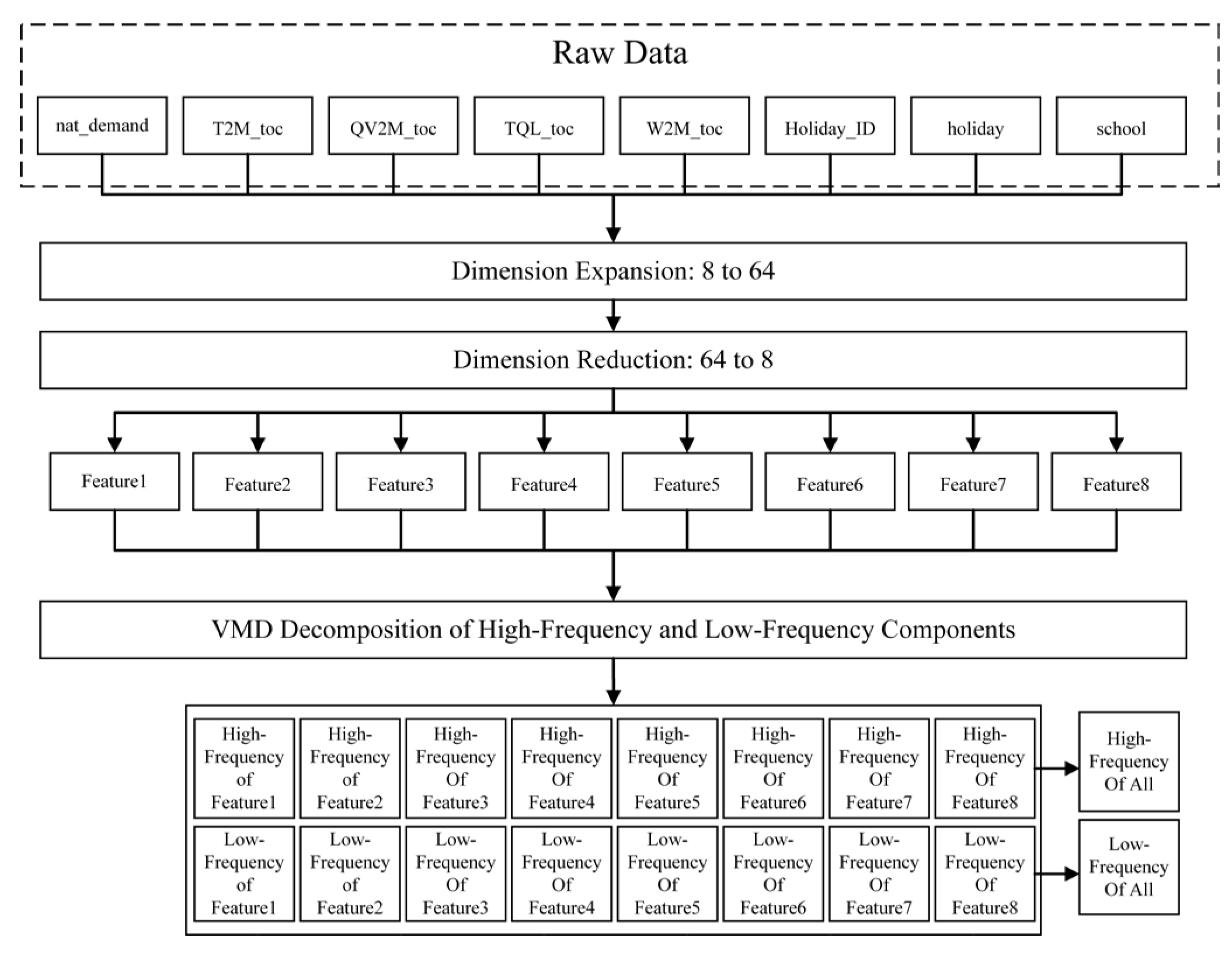
To address this issue, this paper proposes an innovative feature engineering framework. First, a neural network-based dimensionality expansion operation is applied to integrate low-correlation features with the original load data. Then, a dimensionality reduction step restores the feature space to a lower dimension. Subsequently, Variational Mode Decomposition is employed to perform high- and low-frequency signal decomposition on the reduced-dimensional data. The overall procedure of the proposed method is illustrated in Figure 1.
The proposed feature engineering framework integrates Pearson correlation analysis, neural network-based dimensionality expansion and reconstruction, as well as Variational Mode Decomposition. As illustrated in Figure 1, the original input consists of eight features, with the load variable serving as the core prediction target. To better capture the potential interactions among features, the original features are first projected into a higher-dimensional representation space. Specifically, nonlinear coupling relationships between each feature and the remaining features are considered, forming 56 pairwise interaction terms. Additionally, temporal associations within each feature across different time points are incorporated, resulting in a total of 64 dimensions in the expanded space. This representation facilitates the modeling of complex relationships that are difficult to capture in the original space and enhances the model’s capacity to perceive nonlinear structures. Subsequently, a dimensionality reduction step is applied to compress the high-dimensional representation back to eight dimensions, aligning with the original in-put size. This reduction retains key structural information while eliminating redundancy and ensuring consistency in feature dimensionality for subsequent modeling. Together, the expansion and reduction processes constitute a feature reconstruction mechanism that significantly improves the model’s ability to represent and utilize the input data.
Following feature reconstruction, the reduced features are further decomposed into high- and low-frequency components using VMD, enabling the extraction of discriminative frequency patterns. By separating long-term trends from short-term fluctuations, the model can more effectively learn load variation patterns at different temporal scales, thereby enhancing its capacity to characterize underlying load dynamics. Overall, this feature engineering approach improves feature quality while compressing redundant in-formation, ultimately contributing to better model generalization and predictive performance.
The experiments in this study were conducted using the Panama Short-Term Power Load Forecasting Dataset, obtained from the Kaggle platform. This is a typical multi-feature dataset widely used for evaluating load forecasting models. It contains hourly power load data collected over a five-year period, along with relevant environmental variables such as temperature, humidity, and wind speed. In addition, the dataset includes weather information from surrounding cities. For experimental purposes, we selected data from 1 January 2019 to 1 June 2020, and excluded the climate variables from neighboring cities to focus exclusively on load forecasting for the Panama region. The final dataset consists of 8 feature variables, each with 12,409 hourly records, totaling 99,272 data points. The names and descriptions of all feature variables are provided in Table 1.
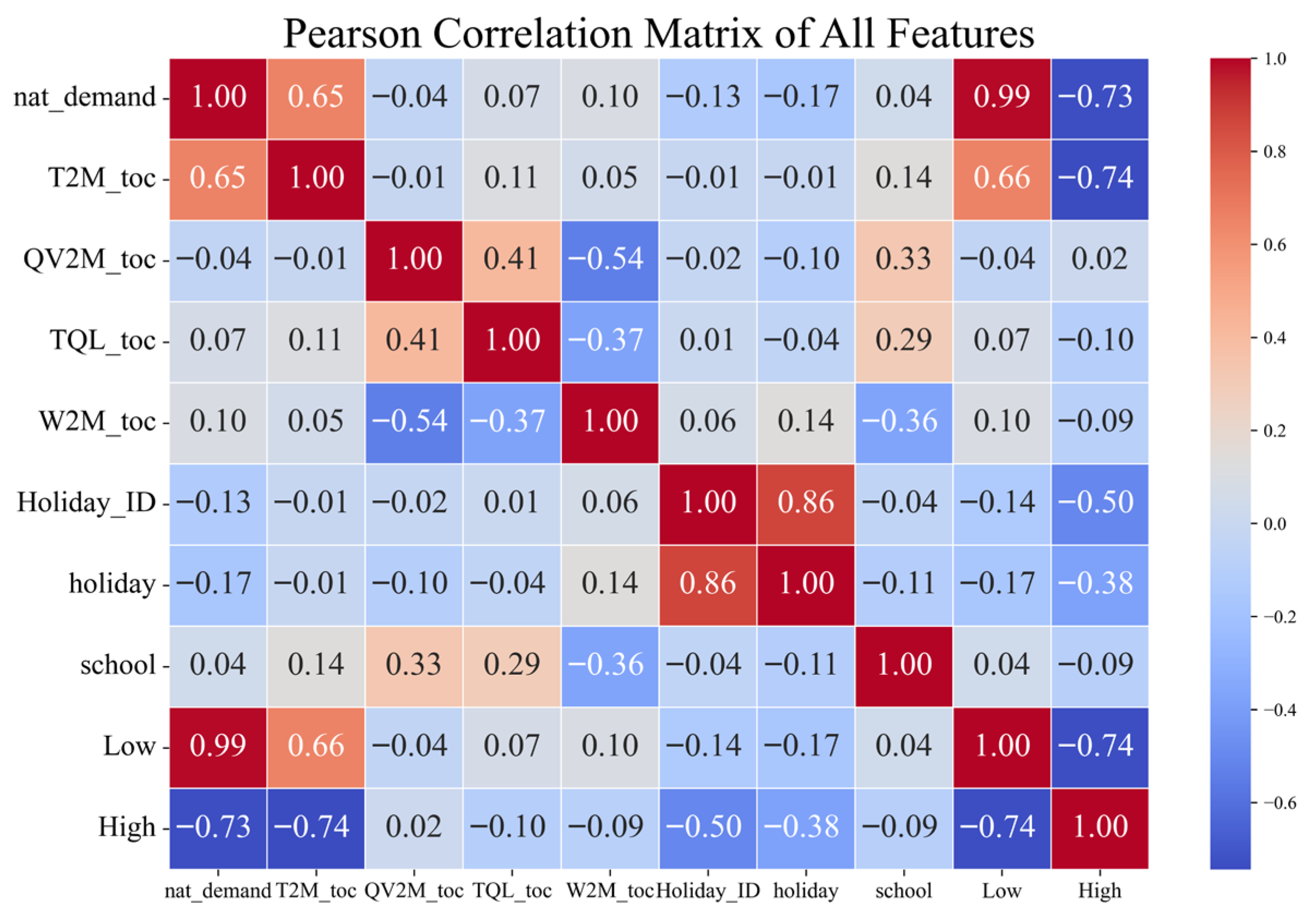
To validate the effectiveness of the proposed feature engineering method, this study employs the Pearson correlation coefficient to measure the linear correlation between each feature and the target variable. A correlation heatmap is also constructed to intuitively illustrate the relationships between the features and the power load. By computing the correlation coefficients, it becomes possible to effectively identify features that are strongly associated with the load variable. The Pearson correlation coefficient is defined as follows:
ρ = i = 1 N x i x ¯ y i y ¯ i = 1 N x i x ¯ 2 i = 1 N y i y ¯ 2  
In Equation (1), ρ denotes the Pearson correlation coefficient; x i and y i represent any two features, and x ¯ and y ¯ indicate the mean values of the corresponding features. Figure 2 illustrates the correlation heatmap, where the color scale ranges from dark blue to dark red, corresponding to correlation coefficients ranging from −1 to 1, respectively. In the heatmap, dark red indicates a strong positive correlation between a feature and the target variable, while dark blue indicates a strong negative correlation. The exact correlation values can be obtained directly from the annotated data in the figure.
As shown in Figure 2, in the original dataset, the power load exhibits the highest correlation with temperature, with a Pearson correlation coefficient of 0.65, indicating a significant positive relationship between the two. Temperature changes have a strong impact on power load; for instance, during cold winters or hot summers, increased use of heating or air conditioning can lead to a rise in electricity demand. In contrast, the correlations between power load and other features are generally low and close to zero. In particular, humidity and wind speed show weak associations with load variations, as their fluctuations typically do not directly affect power demand. Additionally, holiday-related features such as Holiday_ID and holiday also exhibit limited correlation with load, suggesting that their direct influence on load changes is minimal.
The figure also presents the correlations between the power load and the low-frequency and high-frequency components extracted through feature engineering, which are 0.99 and −0.73, respectively. The strong positive correlation of the low-frequency component indicates that it effectively captures the long-term trend of load variation, while the significant negative correlation of the high-frequency component reflects a consistent inverse relationship with short-term fluctuations. This processing approach facilitates the separation of long-term trends from short-term disturbances, enhancing the model’s responsiveness to information across different temporal scales. Table 2 lists the final feature set used for model input. These features, after reconstruction and frequency-domain decomposition, are better suited for characterizing load variation patterns and provide a more discriminative foundation for subsequent model training.
As shown in Table 1 and Table 2, after applying the feature engineering process, the number of features was reduced from 8 to 4, and the total number of data points decreased from 99,272 to 49,636, significantly reducing the dataset size. The load and temperature features were directly retained from the original dataset, thereby eliminating the risk of data leakage. Furthermore, the low- and high-frequency components generated by VMD preserve the same time step as the original data, ensuring continuity of the time series.
To verify the effectiveness of the proposed feature engineering method, this study selected TCN, LSTM, and GRU as benchmark models, and conducted a comparison between the original dataset and the dataset processed by feature engineering. Both datasets were split with 70% used for the training set and 30% for the test set. Specifically, the original dataset contains 69,490 training data points and 29,782 test data points; while the processed dataset includes 34,745 training data points and 14,891 test data points.
To evaluate the performance of each model on the dataset, this study employs three commonly used evaluation metrics—Root Mean Square Error (RMSE), Coefficient of Determination (R2), and Mean Absolute Error (MAE). Specifically, RMSE is used to measure the prediction accuracy of the model, R2 reflects the model’s ability to explain the variability in the data, and MAE represents the average absolute difference between the predicted values and the actual values. The mathematical definitions of these metrics are provided below:
R M S E = 1 n i = 1 n ( y i y ^ i ) 2
R 2 = 1 i = 1 n ( y i y ^ i ) 2 i = 1 n ( y i y ¯ ) 2
M A E = 1 n i = 1 n y i y ^ i
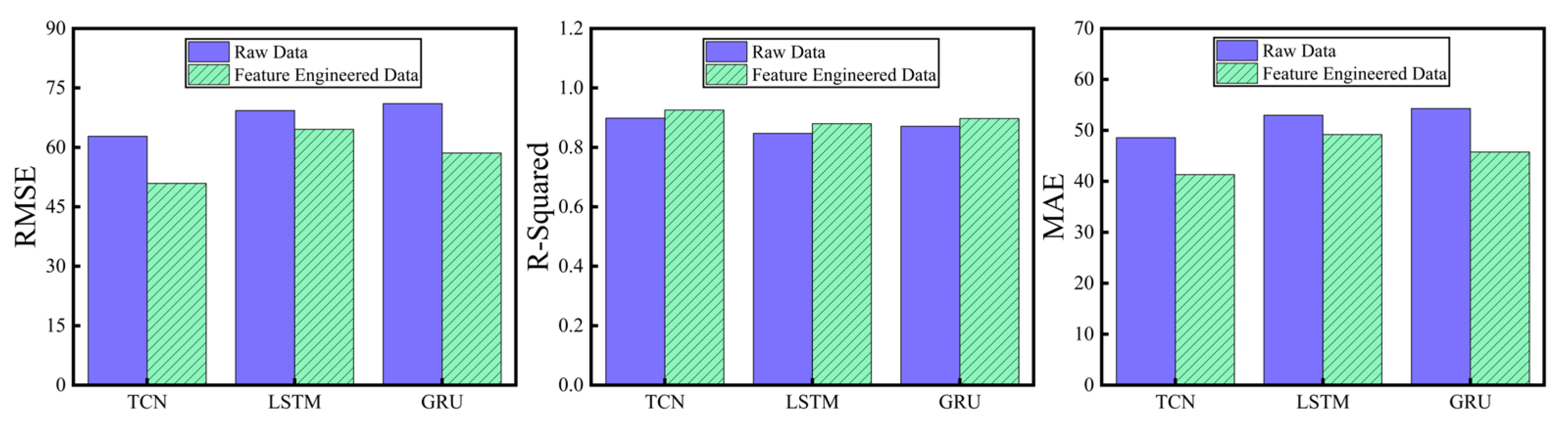
where y i denotes the actual value, y ^ i is the predicted value, y ¯ represents the mean of actual values, and n is the number of samples. Figure 3 illustrates the performance of the two datasets on the three benchmark models, with the datasets represented by different colors as indicated in the legend. Table 3 provides the corresponding numerical comparison.
As shown in Table 3, feature engineering significantly improved the prediction performance of all baseline models. For the TCN model, the RMSE decreased from 62.7795 to 50.9168, while the R2 increased from 0.8983 to 0.9256, indicating that feature engineering played a crucial role in enhancing prediction accuracy and improving model fitting. In addition, both the MAE and RMSE values of all three baseline models were reduced, further confirming the effectiveness of feature engineering in minimizing prediction errors. Combined with the analysis of the correlation heatmap and the validation results of the baseline models, the proposed feature engineering approach significantly improved the accuracy of load forecasting, fully demonstrating its effectiveness in optimizing predictive performance.

2.2. African Vultures Optimization Algorithm

The African Vultures Optimization Algorithm (AVOA) is a novel meta-heuristic algorithm inspired by the hunger-driven foraging behavior of African vultures. It was proposed by Abdollahzadeh et al. for solving global optimization problems.

2.2.1. Original AVOA Algorithm

The original AVOA algorithm can be summarized into the following four components:
1.
Random initialization of the vulture population:
The   Architectural   Design   of   TCN   P i   = l b + r a n d ( 0 , 1 ) × ( u b l b )
2.
Determine the optimal vulture individuals:
Select the vultures with the best fitness values as Leaders BestVulture 1 and BestVulture 2 :
R ( i ) = BestVulture 1 , p i = L 1 BestVulture 2 , p i = L 2
Here, L 1 and L 2 are parameters to be measured before the search operation, both ranging from 0 to 1, and satisfying the condition L 1   + L 2   = 1 . Subsequently, Equation (7) is used to select the best solution for each group, thereby determining the probability of selecting the optimal solution.
p i = F i i = 1 N F i
3.
Exploration Phase:
The hunger rate governs the dynamic transition between the exploration and exploitation phases and serves as the core scheduling parameter of AVOA. Its variation is jointly determined by a time adjustment function t and a random variable z , as follows:
t = h × ( sin w ( π 2 × i t e r a t i o n i max i t e r a t i o n s ) + cos ( π 2 × i t e r a t i o n i max i t e r a t i o n s ) 1 )
F = ( 2 × r a n d 1 + 1 ) × z × ( 1 i t e r a t i o n i max i t e r a t i o n s ) + t
In Equations (8) and (9), iter denotes the current iteration number, and i t e r a t i o n i represents the maximum number of iterations. The parameter z is a perturbation control variable, defined within the range z 1 , 1 , and it changes with each iteration. Parameters h and w are constants used to control the shape of the hunger curve. The variable t is introduced to enhance the algorithm’s ability to escape from local optima. F is used to determine the phase transition; when F 1 , the algorithm enters the exploration phase, whereas when F < 1 , it switches to the exploitation phase.
During the exploration phase, vultures search broadly for potential food sources. The algorithm selects between two distinct random search patterns based on a probability parameter P 1 , which is a random value generated within the range [0, 1] prior to executing the search operation. As shown in Equation (10), if the value of r a n d P 1 is greater than or equal to the parameter P 1 , Equation (11) is adopted; otherwise, Equation (13) is applied.
P ( i + 1 ) = E q u a t i o n ( 11 ) , P 1 r a n d P 1 E q u a t i o n ( 13 ) , P 1 < r a n d P 1
Mechanism 1: Distance-Driven Search
P ( i + 1 ) = R ( i ) D ( i ) × F
D ( i ) = X × R ( i ) P ( i )
In this mechanism, P ( i + 1 ) represents the position vector of the vulture in the next iteration, and F is the hunger rate parameter obtained from Equation (9) in the current iteration. In Equation (12), R ( i ) denotes one of the best vultures selected using Equation (6) during the current iteration. X is a coefficient vector used to introduce randomness, calculated as X = 2 × r a n d , where r a n d is a random number between 0 and 1, simulating the vulture’s behavior of approaching or moving away from the reference target in a random direction. P ( i ) is the current position vector of the vulture.
Mechanism 2: Random Offset Search
P ( i + 1 ) = R ( i ) F + r a n d 2   × ( ( u b l b ) × r a n d 3   + l b )
r a n d 2 is a random value between 0 and 1. In Mechanism 2, new positions are generated randomly over the global search space to enhance the diversity of the search.
4.
Exploitation Phase:
When F < 1 , the algorithm enters the exploitation phase, indicating that the vulture has discovered a potential food source and begins to encircle or hunt. This phase is divided into two states: moderate satiety and intense hunger. Each state involves two key parameters: P 2 and P 3 . Specifically, P 2 is used in the moderate satiety state, while P 3 is used in the intense hunger state. Before entering the exploitation phase, both parameters are initialized with values of 0 and 1, respectively.
State 1: Moderate Satiety State ( 0.5 F < 1 )
At the beginning of the exploitation phase, a random number r a n d P 2 is generated between 0 and 1. If this number is greater than or equal to parameter P 2 , the vulture performs an encircling competition strategy. Otherwise, a spiral flight strategy is applied:
P ( i + 1 ) = E q u a t i o n ( 15 ) , P 2 r a n d P 2 E q u a t i o n ( 19 ) , P 2 < r a n d P 2
Mechanism 1: Encircling Competition
P ( i + 1 ) = D ( i ) × ( F + r a n d 4 ) d ( t )
d ( t ) = R ( i ) P ( i )
In Equation (15), D ( i ) is calculated using Equation (12), and F is obtained from Equation (9). The variable r a n d 4 generates a random value between 0 and 1, which is used to introduce stochastic variability in the scaling factor.
Mechanism 2: Spiral Flight
S 1 = R ( i ) × ( rand 5 × P ( i ) 2 π ) × cos ( P ( i ) )
S 2 = R ( i ) × ( rand 6 × P ( i ) 2 π ) × sin ( P ( i ) )
P ( i + 1 ) = R ( i ) ( S 1 + S 2 )
R ( i ) denotes the position vector of one of the two best vultures in the current iteration, as determined by Equation (6). The functions cos and sin represent the standard sine and cosine functions, respectively. The variables r a n d 5 and r a n d 6 are random numbers ranging from 0 to 1. By computing S 1 and S 2 , the position of the vulture is ultimately updated using Equation (19).
State 2: Severe Hunger State ( F < 0.5 )
When vultures are in a state of extreme hunger, they exhibit more aggressive attacking or convergence behaviors. In this case, the algorithm selects different mechanisms based on the value of P 3 . The variable r a n d P 3 is a random number between 0 and 1.
P ( i + 1 ) = E q u a t i o n ( 23 ) , P 3 r a n d P 3 E q u a t i o n ( 24 ) , P 3 < r a n d P 3
Mechanism 1: Aggregation
A 1 = B e s t V u l t u r e 1 ( i ) B e s t V u l t u r e 1 ( i ) × P ( i ) B e s t V u l t u r e 1 ( i ) P ( i ) 2 × F
A 2 = B e s t V u l t u r e 2 ( i ) B e s t V u l t u r e 2 ( i ) × P ( i ) B e s t V u l t u r e 2 ( i ) P ( i ) 2 × F
P ( i + 1 ) = A 1 + A 2 2
In Equations (21) and (22), B e s t V u l t u r e 1 ( i ) represents the first group of best-performing vultures in the current iteration, and B e s t V u l t u r e 2 ( i ) denotes the second group of best-performing vultures. Finally, all vultures are aggregated using Equation (23) to obtain the updated position P ( i + 1 ) for the next iteration.
Mechanism 2: Attack
P ( i + 1 ) = R ( i ) d ( t ) × F × L e v y ( d )
L e v y ( x ) = 0.01 × u × σ v 1 β
σ = Γ ( 1 + β ) × sin ( β 2 π ) Γ ( ( 1 + β ) 2 ) × β × 2 ( β 1 ) 2 1 β
In Equation (24), d denotes the problem dimension. In Equation (25), u and v are random numbers uniformly distributed in the range [0, 1], a is a constant fixed at 1.5, and the value of β is calculated according to Equation (26).
The computational complexity of the original AVOA algorithm depends on three fundamental components: initialization, fitness evaluation, and vulture position update. Therefore, its overall time complexity can be expressed as:
O ( N × ( T + T D ) )
where N is the population size, T is the maximum number of iterations, and D is the problem dimension.

2.2.2. Improved African Vulture Optimization Algorithm

To address the limitations of the traditional African Vulture Optimization Algorithm—including strong randomness in population initialization, insufficient balance between exploration and exploitation due to fixed parameters, and the decline of population diversity in later stages—this paper proposes an Improved African Vulture Optimization Algorithm. While retaining the overall framework and bio-inspired characteristics of the original algorithm, IAVOA introduces targeted enhancements from the following three aspects:
1.
A population initialization strategy based on Perturbation-Enhanced Dynamic Tent Mapping is designed to improve the uniformity of the initial distribution and enhance global exploration capabilities;
2.
An Adaptive Parameter Control mechanism is incorporated into the AVOA to dynamically balance the exploration and exploitation phases;
3.
An Elite Retention and Migration mechanism is introduced to prevent the loss of high-quality individuals and maintain population diversity.
1.
Perturbation-Enhanced Dynamic Tent Mapping
The original population initialization method may lead to individual clustering or uneven coverage in high-dimensional spaces, leading to insufficient diversity in the early search phase. To enhance the spatial uniformity and global exploration potential of the initial population in optimization algorithms, this paper proposes a Perturbation-Enhanced Dynamic Tent Mapping based on the traditional Tent chaotic map.
By incorporating time-dependent parameter control and slight random perturbation mechanisms, this method preserves the chaotic characteristics while significantly improving the uniform distribution of initial individuals in the search space, thereby avoiding the banded clustering problem typically caused by standard Tent sequences.
1.
Dynamic Parameter Design:
As one of the classical models in nonlinear dynamics, the Tent map is a piecewise linear transformation widely used in the study of chaotic systems. Its basic form transforms the input value x n through a control parameter μ , and the mapping is defined as follows:
x n + 1 = μ x n , 0 x n 0.5 μ ( 1 x n ) , 0.5 < x n 1
Here, μ is the control parameter that determines the behavioral characteristics of the mapping. As the value of μ gradually increases, the system transitions from ordered periodic behavior to a chaotic state, and this transition becomes particularly pronounced.
Due to its simple mathematical structure, the Tent map provides an intuitive representation of chaotic behavior in nonlinear systems and effectively reveals the transition between periodicity and chaos. As a result, it has been widely used in cryptography and pseudo-random number generation. However, owing to its limited parameter range and relatively simple structure, the Tent map exhibits certain limitations in modeling complex systems. To maintain the chaotic properties of the Tent map while improving the uniformity of the initial population distribution, this paper introduces an enhanced version of the Tent mapping. The improved formulation is defined as follows:
x n + 1 = x n μ ( t ) , x n < μ ( t ) 1 x n 1 μ ( t ) , x n > μ ( t )
Here, μ ( t ) is the time-dependent control parameter, defined as μ ( t ) = μ 0   + Δ μ t T   , μ 0   = 0.5 , 0.1 Δ μ 0.2 ; Δ μ is the amplitude of the dynamic perturbation; t represents the current iteration number; and T denotes the maximum number of iterations.
This dynamic structure allows the Tent map to continuously shift its axis of symmetry during the iterative process, thereby generating a periodic distribution drift on a global scale. Such behavior enhances the diversity of the search in the early stages of the optimization process.
2.
Perturbation-Enhanced Mechanism:
To further disrupt the aggregation characteristics of deterministic chaotic trajectories, a small perturbation term is introduced after each iteration:
x n + 1 = x n μ ( t ) + ε U ( 1 , 1 ) , x n < μ ( t ) 1 x n 1 μ ( t ) + ε U ( 1 , 1 ) , x n μ ( t )
Here, U 1 , 1 denotes a random variable that follows a uniform distribution over the interval [−1, 1]; ε is the perturbation intensity, where ε [ 0.01 , 0.05 ] . By applying a slight random perturbation to the mapped value, the perturbation term effectively eliminates autocorrelation among trajectories, resulting in a more dispersed distribution of individual positions.
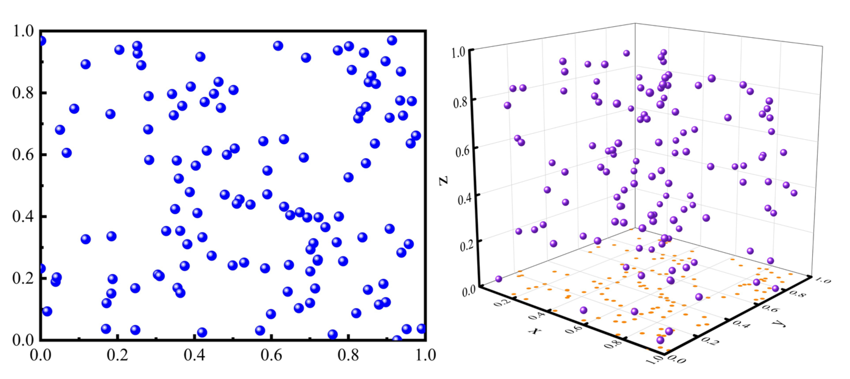
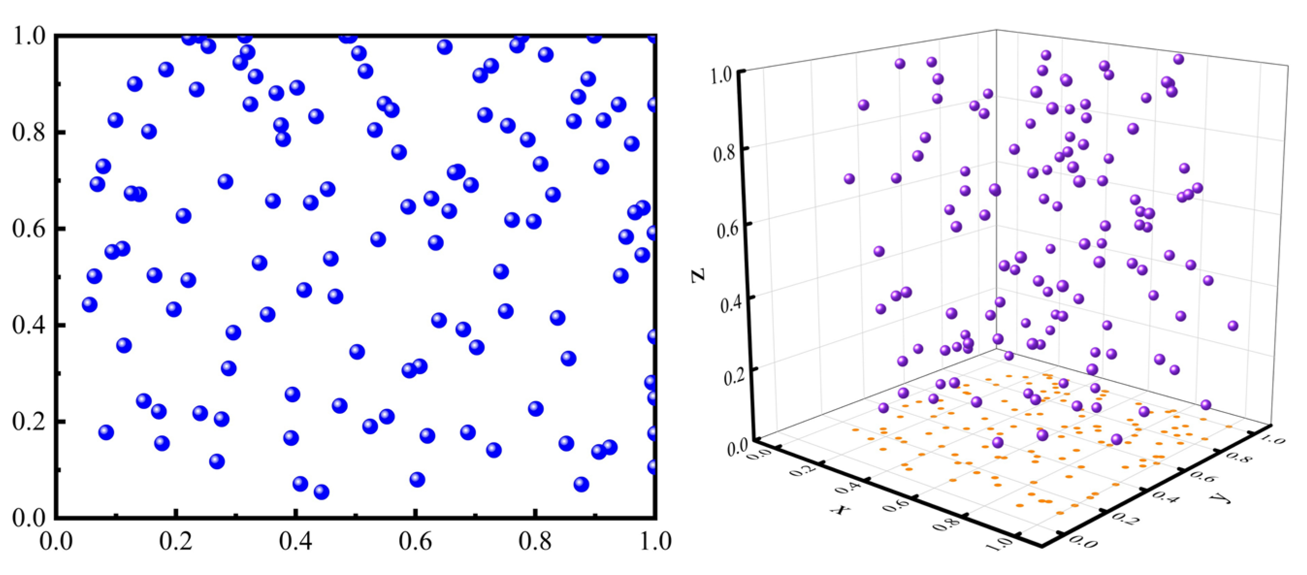
Figure 4 and Figure 5 illustrate the population sample distributions generated by random initialization and PDTM-based initialization in two-dimensional and three-dimensional spaces, respectively. The colors in the figures are used solely for visualization enhancement and do not convey any specific meaning. As shown in the figures, the population generated by random initialization exhibits clear non-uniformity, characterized by multiple dense and sparse regions interspersed throughout the space, which hinders effective coverage of the entire search space. In contrast, the proposed PDTM-based initialization method significantly improves the spatial uniformity of the population distribution, enhancing not only the diversity of the initial population but also providing a better starting point for the optimization process.
The aforementioned improvements enable PDTM to retain the inherent nonlinear dynamic characteristics of chaotic sequences while enhancing its ability to regulate distribution structure. This facilitates the generation of a more exploratory initial population layout, introducing higher initial perturbation and better spatial coverage for the subsequent search process. It is important to note that in this study, PDTM is applied solely during the population initialization phase of the optimization algorithm. Its primary objective is to generate a more randomized and uniformly distributed set of initial individuals, thereby enhancing the diversity of search starting points and reducing initialization bias. Under this one-time usage setting, the stochasticity of PDTM serves as a desirable property for improving initialization quality rather than a flaw.
3.
Adaptive Control Parameter Mechanism
In the original AVOA, fixed parameters (such as L 1 , L 2 , P 1 , P 2 , P 3 , w ) are used throughout the optimization process. Specifically, L 1 and L 2 determine the flight search range of vultures; P 1 , P 2 , and P 3 adjust the balance between exploration and exploitation; the parameter w controls the variation of the hunger rate and affects the update speed. However, fixing these parameters throughout the optimization process limits the algorithm’s ability to adapt to problem-specific requirements at different stages. As a result, the algorithm may exhibit excessive exploration or insufficient local exploitation in the later iterations, thereby compromising the convergence performance.
To address this limitation, a dynamic adaptive parameter adjustment mechanism is introduced in this study. This mechanism enables the algorithm to maintain a proper balance between exploration and exploitation phases, thereby enhancing both global search capability and local optimization efficiency. The updated parameter adjustment equations are formulated as follows:
w ( t ) = w max t T ( w max w min )
L 1 ( t ) = L 1 _ max t T ( L 1 _ max L 1 _ min ) , L 2 ( t ) = 1 L 1 ( t )
P i ( t ) = P i + α sin ( π t T ) , i 1 , 2 , 3
In Equation (8), the original algorithm employs a fixed constant w = 2 , causing the oscillation range of the hunger rate F to remain constant throughout the entire iteration process. In contrast, IAVOA replaces it with a linearly decreasing function ω ( t ) , as defined in Equation (31), allowing the oscillation amplitude of the hunger rate function to gradually converge. This adaptive adjustment enables the algorithm to exhibit strong global exploration in the early stages and stable local exploitation in the later stages.
In Equation (6), the parameters L 1 and L 2 in the original algorithm are fixed and randomly generated before the algorithm is executed, which maintains a balanced population distribution during the search process. As shown in Equation (32), the improved version adopts a time-dependent L 1 ( t ) that decreases over iterations, promoting more intensive exploration at the beginning and progressively enhancing local exploitation in the later stages.
During the exploration and exploitation processes, the original algorithm uses fixed constants for P 1 , P 2 , and P 3 , resulting in constant behavior selection probabilities throughout the search. In the improved version, a time-varying oscillatory function P i ( t ) is introduced, as defined in Equation (33), which enables a cyclic and dynamic transition between exploration and exploitation phases. This mechanism periodically “reactivates” the exploration stage during iterations, effectively helping the algorithm escape from local optima.
These dynamic adjustment mechanisms enable the algorithm to enhance its global search ability during the initial iterations and gradually shift toward local refinement in the later phases. This smooth transition optimizes the balance between exploration and exploitation, improves the algorithm’s adaptability, and ultimately enhances the convergence stability.
4.
Elite Retention and Migration Mechanism
In the original AVOA, the update of individuals relies entirely on the current population, lacking memory of historically superior solutions. This often leads to the loss of valuable information and population homogenization. To address this issue, this study introduces an elite retention and migration mechanism. In each generation, the top k % of the best-performing individuals are retained to form an elite set E , and a migration-based update is executed every τ iterations as follows:
X n e w = X e + λ ( t ) ( r a n d 0.5 )
where X n e w denotes the individual with the best fitness in the elite set, and X e represents the optimal solution among elite individuals. The migration coefficient λ ( t ) = λ 0 ( 1 t / T ) is gradually decaying over iterations. The parameter settings are: k = 10 , τ = 1 , and λ 0 = 0.2 .
The elite retention and migration mechanism simulates the natural selection process by preserving a certain number of high-quality solutions and replacing the worst-performing individuals. This strategy not only increases the probability of convergence toward the global optimum but also effectively maintains population diversity, thereby avoiding premature convergence. By replacing the worst-performing k % of individuals, the algorithm mimics the migration and aggregation behavior of vultures, ensuring the preservation of historically optimal solutions while maintaining population diversity and global search capability.
5.
Overall Workflow of IAVOA
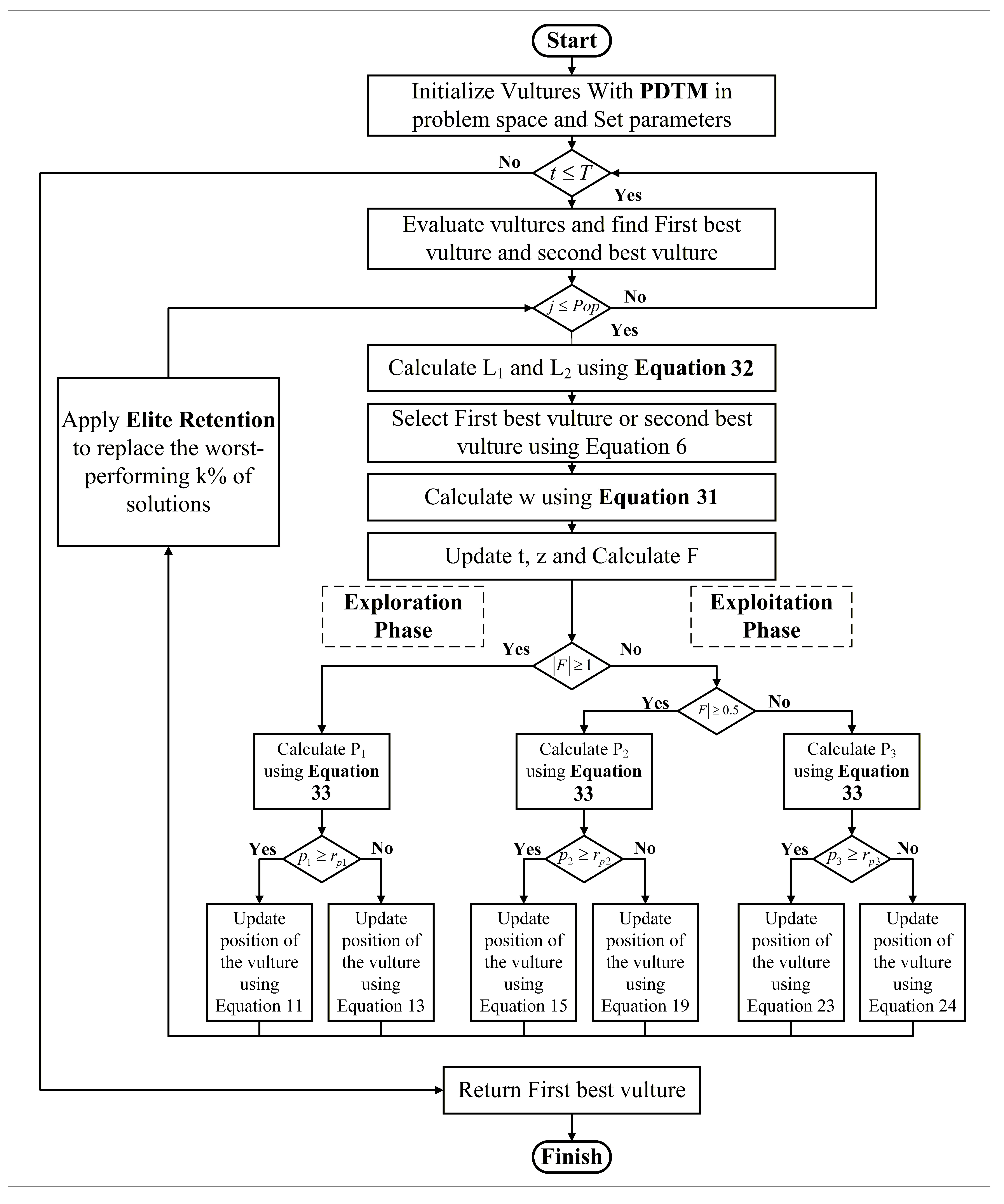
Figure 6 illustrates the overall workflow of IAVOA. To establish an effective balance between search space distribution and population strategy, IAVOA emphasizes different optimization priorities across three stages: initialization, search iteration, and convergence control. In the initialization stage, Perturbation-Enhanced Dynamic Tent Mapping (PDTM) is introduced to improve the coverage and uniformity of the initial population. During the search and iteration phase, an adaptive control parameter mechanism is employed to dynamically adjust individual behavior, achieving a balanced transition between exploration and exploitation. In the convergence control stage, an elite retention and migration mechanism is incorporated, using a guiding strategy to enhance convergence accuracy and prevent premature convergence to local optima. Overall, IAVOA achieves comprehensive optimization of search efficiency, solution space coverage, and convergence stability through the coordinated design of initialization perturbation, adaptive regulation, and elite-guided strategies.

2.2.3. Testing the IAVOA

To verify the effectiveness and stability of the IAVOA algorithm, two commonly used benchmark test functions are selected in this study: the Schwefel Problem 2.21 and the Generalized Penalized Function. These two functions represent unimodal and multimodal optimization problems, respectively, and are capable of comprehensively evaluating the algorithm’s performance across different types of optimization tasks.
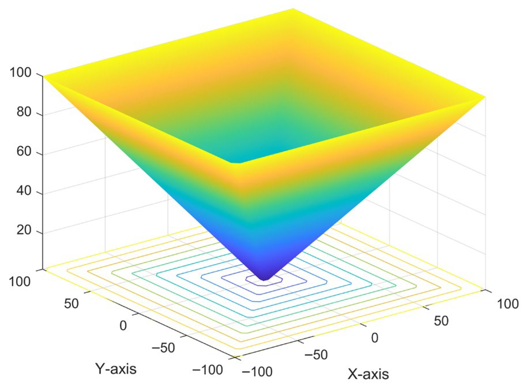
The Schwefel Problem 2.21 is a typical unimodal function characterized by its symmetric shape and gentle gradient. Its global minimum is zero and located at the origin. However, due to the weak gradient information near the optimal solution, the algorithm may converge slowly when solving this function. Therefore, Schwefel Problem 2.21 is well-suited for testing the local search ability and convergence precision of optimization algorithms. The surface of this function is illustrated in Figure 7, and the corresponding formula is defined as follows:
f x = max x i , 1 i 30 , 100 x i 100
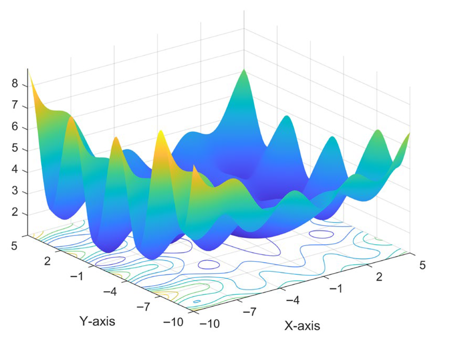
The Generalized Penalized Function is a multimodal and nonlinear function characterized by a complex boundary structure and a large number of local optima. These features make the optimization process highly challenging. This function is commonly used to evaluate an algorithm’s global search capability, its ability to escape from local optima, and its adaptability to constrained conditions. An example of the function’s surface is shown in Figure 8. It is worth noting that the colors and projections in Figure 7 and Figure 8 are used solely for visual enhancement and do not carry any specific meaning.
Let x = x 1 , x 2 , x d R d , and the function is defined as follows:
f x = π 30 10 sin 2 π y 1 + i = 1 29 y i 1 2 1 + 10 sin 2 π y i + 1 + y d 1 2 + i = 1 30 U x i , 10 , 100 , 4
where 50 x i 50 , and the variable transformation y i is computed as follows:
y i = 1 + x i + 1 4 , i = 1 , 2 , , d
The penalty function U x i , a , k , m is defined as
U x i , a , k , m = k x i a m i f   x i > a 0 i f   x i a k x i a m i f   x i < a
In this study, several representative optimization algorithms were selected for comparative experiments, including the Enhanced Whale Optimization Algorithm (EWOA) [20], Multi-Verse Optimizer (MVO) [21], Chameleon Swarm Algorithm (CSA) [22], Improved Grey Wolf Optimizer (IGWO) [23], and Beluga Whale Optimization (BWO) [24]. These algorithms were compared against the baseline African Vultures Optimization Algorithm to verify the superiority of the proposed algorithm.
EWOA and MVO demonstrate strong capabilities in escaping local optima: the former enhances global search ability through an adaptive mechanism, while the latter improves solution diversity via a multi-version strategy. CSA and IGWO exhibit advantages in global exploration: CSA improves adaptability by dynamically adjusting its search strategy, whereas IGWO enhances convergence accuracy through a modified leader selection mechanism. BWO performs well in high-dimensional and complex problems by optimizing the search process through information sharing, thereby improving the robustness of the algorithm.
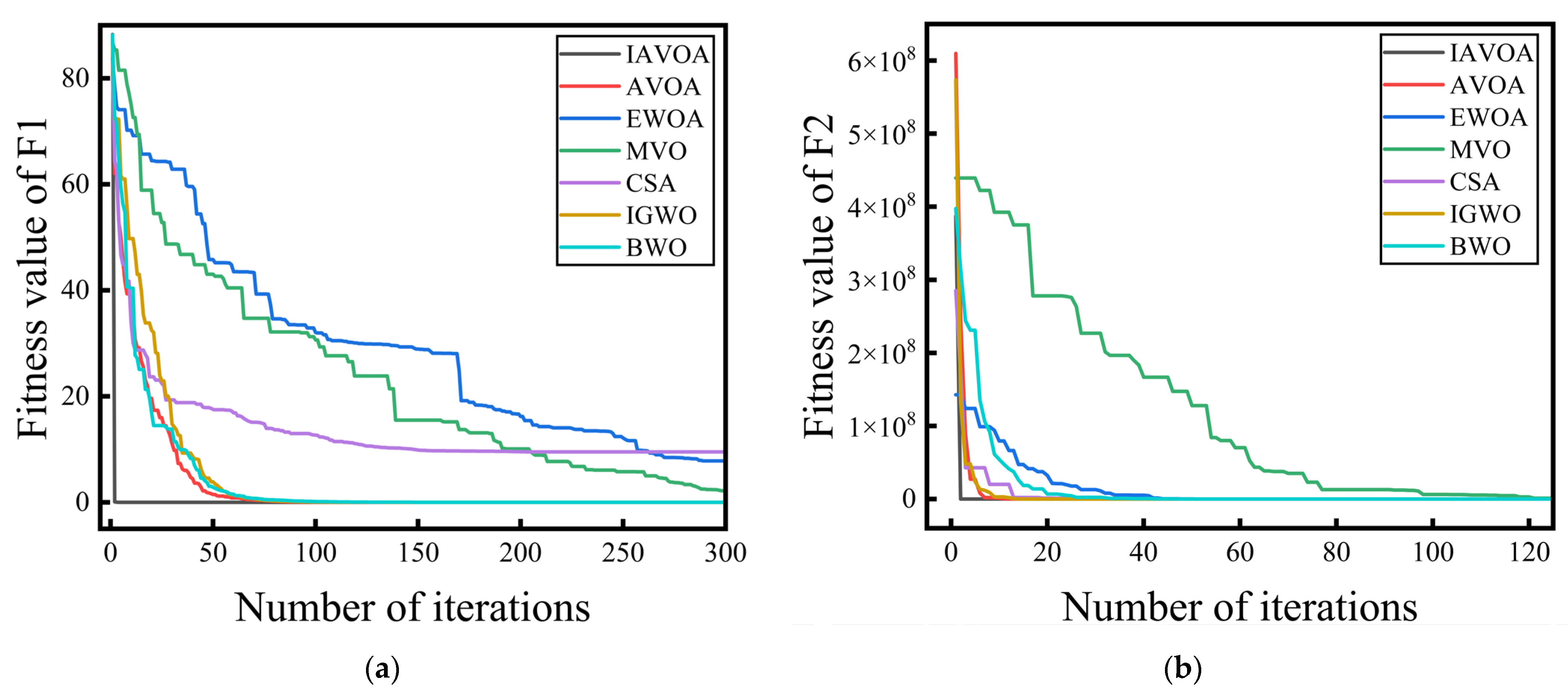
For all algorithms, the initial population size was set to 50, and the number of iterations was fixed at 300. The experimental results are presented in Table 4 and Table 5, and the optimization processes on the two benchmark functions are illustrated in Figure 9a and Figure 9b, respectively. The colors of the curves represent different optimization algorithms, as indicated in the figure legends.
As illustrated in Figure 9a, for the unimodal function F1 (Schwefel’s Problem 2.21), the IAVOA algorithm rapidly descends to the minimum value, demonstrating an exceptionally high convergence speed. This characteristic indicates that IAVOA can effectively avoid excessive exploration in regions with weak gradient information and can swiftly locate the global optimum.
Benefiting from its multi-stage cooperative control mechanism, IAVOA achieves a significant reduction within the first five iterations, showcasing both fast and stable convergence. Compared with other benchmark algorithms, IAVOA reaches near-optimal solutions the earliest, highlighting its superior global search capability and convergence efficiency. This optimization task confirms IAVOA’s superiority in unimodal function optimization, particularly in handling flat-gradient regions.
In contrast, the original AVOA and BWO exhibit relatively fast early-stage convergence but slow down in the later stages, lacking sufficient local search capability. While EWOA and MVO possess certain global search abilities, they converge slowly overall and fail to reach the optimal solution within 300 iterations. CSA shows a slow convergence rate during the early stages and struggles to escape from local optima once trapped. IGWO performs well in the later stages but suffers from large fluctuations in the early iterations, indicating limited convergence stability.
In summary, IAVOA demonstrates clear advantages in convergence accuracy, stability, and the ability to escape local optima, validating the effectiveness of the proposed improvements in enhancing the algorithm’s overall performance.
As shown in Figure 9b, in the optimization task of the Generalized Penalized Function, the IAVOA algorithm exhibits a significant convergence advantage. The global minimum of this function differs greatly from the initial solution, which increases the difficulty of the optimization process. Under such circumstances, IAVOA is able to rapidly approach the optimal solution within a short period. This superior performance is attributed to IAVOA’s efficient exploration and exploitation mechanism, enabling fast convergence to the global optimum.
In comparison, the original AVOA, IGWO, and SCA algorithms do not match IAVOA in terms of convergence speed, but they also deliver competitive performance. In particular, IGWO and SCA show advantages in solving multimodal problems. Based on the convergence performance in both the unimodal function F1 and this multimodal function, it can be concluded that AVOA maintains good adaptability in different types of optimization problems. This observation is one of the key reasons for selecting AVOA as the basis for further improvement.
EWOA and BWO also show their respective advantages in multimodal function optimization. Although EWOA converges more slowly, its process is stable and steadily approaches the optimal solution. BWO tends to get trapped in local optima during the early stages, but after several iterations, it accelerates and quickly reaches the global optimum. In contrast, MVO performs relatively poorly. While it is capable of moving gradually toward the optimal solution, it requires significantly more iterations, exceeding 120, whereas other algorithms typically find the optimal solution within 50 iterations.
Table 4 presents the performance of six optimization algorithms on the benchmark test function F1(x). According to the results, IAVOA outperforms the other algorithms in both optimization capability and stability. Specifically, for the F1 function, IAVOA successfully achieved the optimal value of 0, indicating its superior performance in accurately approaching the target solution. In comparison, the best results obtained by AVOA, EWOA, MVO, CSA, IGWO, and BWO were 0.0003, 7.7648, 2.1443, 9.5137, 0.0005, and 0.0008, respectively. Although most of the algorithms approached the optimal value, there were still certain deviations. In particular, EWOA, MVO, and CSA exhibited larger gaps from the theoretical optimum, suggesting relatively weaker global search capabilities and lower efficiency in the solution space of unimodal problems.
In terms of average value, IAVOA achieved the lowest mean of 0.2946, significantly better than the other algorithms. This demonstrates that IAVOA maintained stable and efficient search performance throughout its runs. AVOA obtained an average value of 3.4794, which, although acceptable, was clearly higher than that of IAVOA. The average values of EWOA and MVO were 29.5471 and 23.4527, respectively, indicating that these algorithms are more prone to larger deviations in complex search spaces, which negatively affects the quality of the results. CSA and IGWO also showed relatively high average values, 13.6426 and 4.9123, respectively, reflecting their instability in result quality. BWO achieved an average of 3.9035, which was better than some other algorithms but still exhibited a noticeable level of fluctuation.
The standard deviation is a key indicator for evaluating the stability and robustness of an algorithm. A smaller standard deviation implies more consistent performance. IAVOA had the smallest standard deviation of 5.0963 among all algorithms, indicating its superior stability across multiple runs. AVOA followed with a standard deviation of 10.7954, which was considerably higher than that of IAVOA. The standard deviations of EWOA and MVO were 18.7278 and 19.6106, respectively, suggesting a lack of accuracy. CSA and IGWO showed values of 8.6281 and 13.9570, both relatively high, indicating weaker performance on complex problems. BWO had a standard deviation of 11.9122, which, although slightly better than some algorithms, still did not match the performance of IAVOA.
According to Table 5, in the benchmark test of the multimodal function F2(x), IAVOA successfully achieved the optimal value of 5.7485 × 10⁻¹⁹, which is the smallest among all the compared algorithms. This result indicates that IAVOA possesses a very strong global search capability and highly accurate target approximation ability. In contrast, the best results of AVOA and IGWO were 2.6700 × 10⁻³ and 1.6787 × 10⁻⁵, respectively. Although these values are better than those of other comparative algorithms, they still fall short in precision. EWOA and MVO obtained best results of 0.13999 and 0.80292, respectively, demonstrating poor accuracy and indicating their limited effectiveness in handling complex multimodal optimization tasks.
In terms of average value, IAVOA achieved a mean of 1.2909 × 10⁶, significantly outperforming the other algorithms. This result shows that the algorithm is not only capable of finding the global optimum but also maintains the stability of high-quality solutions across multiple runs. The average values of AVOA and CSA were 3.3718 × 10⁶ and 2.6674 × 10⁶, respectively, which are considerably higher than that of IAVOA. The average values of EWOA and MVO were 6.2435 × 10⁶ and 5.2174 × 10⁷, respectively, indicating that their optimization processes lack stability and are more likely to be affected by local minima, resulting in poorer solution quality.
Finally, with respect to the standard deviation, IAVOA achieved the smallest value of 2.2360 × 10⁷, suggesting that its optimization process is the most balanced. The standard deviations of the other algorithms were all greater than that of IAVOA, reflecting higher variability and a lack of consistency in their performance across multiple runs. In summary, IAVOA demonstrates outstanding performance not only on unimodal problems but also on multimodal problems. Its excellent convergence ability in complex optimization tasks confirms its robustness and adaptability.
The primary computational overhead of IAVOA arises from three components: population initialization, fitness evaluation, and position updating. Since the PDTM mapping and parameter adjustment processes involve only simple arithmetic operations, the time complexity remains the same as that of the original AVOA, which is:
O ( N × ( T + T D ) )
Therefore, IAVOA significantly improves the global search ability and convergence performance of the algorithm without introducing any substantial increase in computational burden.


2.3. EATCN

2.3.1. Original TCN Algorithm

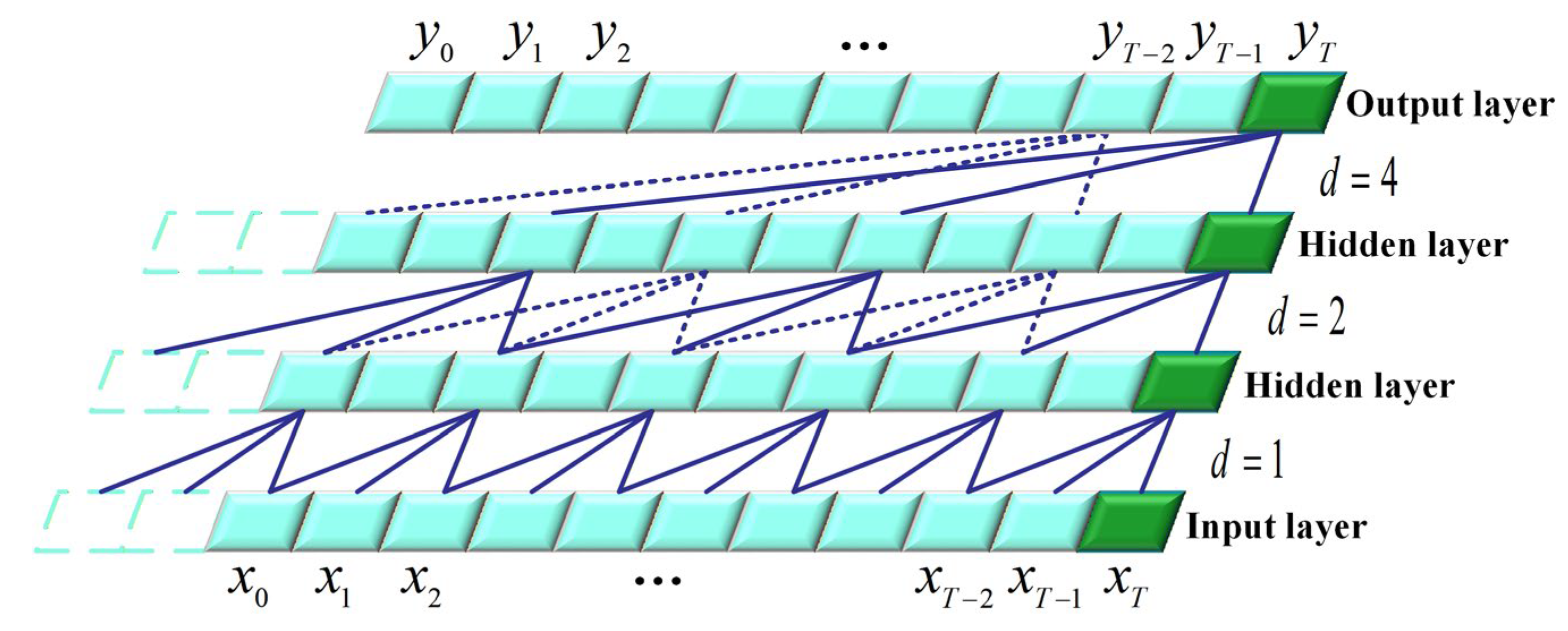
Temporal Convolutional Network is a deep time-series modeling architecture based on one-dimensional convolutions. Dilated convolution is a key component of TCN, designed to exponentially enlarge the receptive field by introducing gaps within the convolutional kernels, thereby capturing long-range dependencies. This mechanism enhances the model’s ability to represent long sequences without increasing the number of parameters. Its structure is illustrated in Figure 10. The colors in the figure are used solely for visualization purposes and do not carry any specific meaning. Compared to recurrent neural networks and their variants, TCN demonstrates higher stability and computational efficiency in modeling long-term dependencies in complex load sequences.
The temporal receptive field of a TCN is jointly determined by the kernel size, dilation rate, and network depth. The core convolutional operation is defined as follows:
F ( t ) = ( x d f ) ( t ) = i = 0 u 1 f ( i ) x t p i
In Equation (40), x denotes the input sequence, represents the convolution operation, d is the dilation factor, u denotes the kernel size, f ( i ) refers to the i -th element of the convolution kernel, and x t p i corresponds to the respective input element.
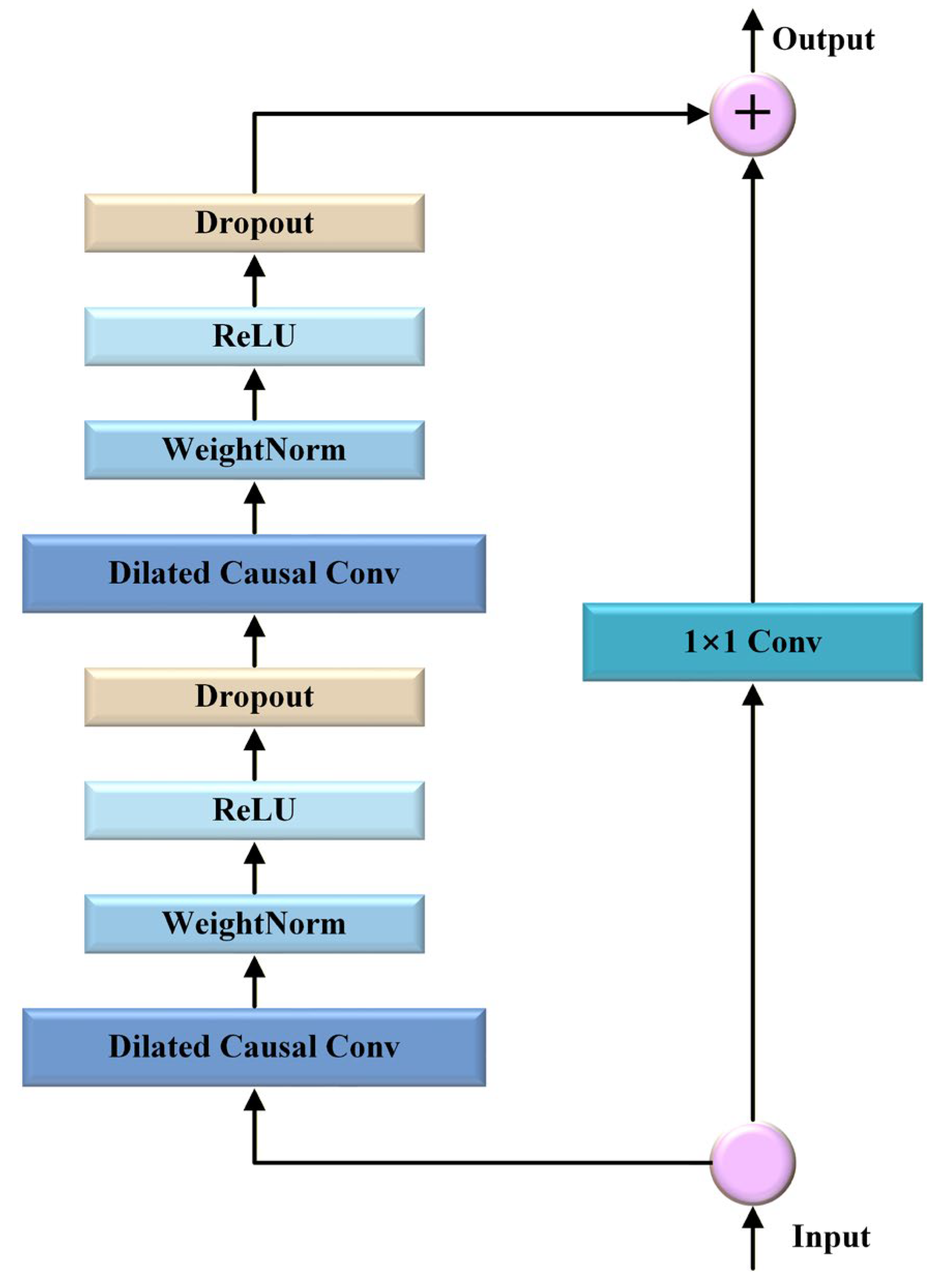
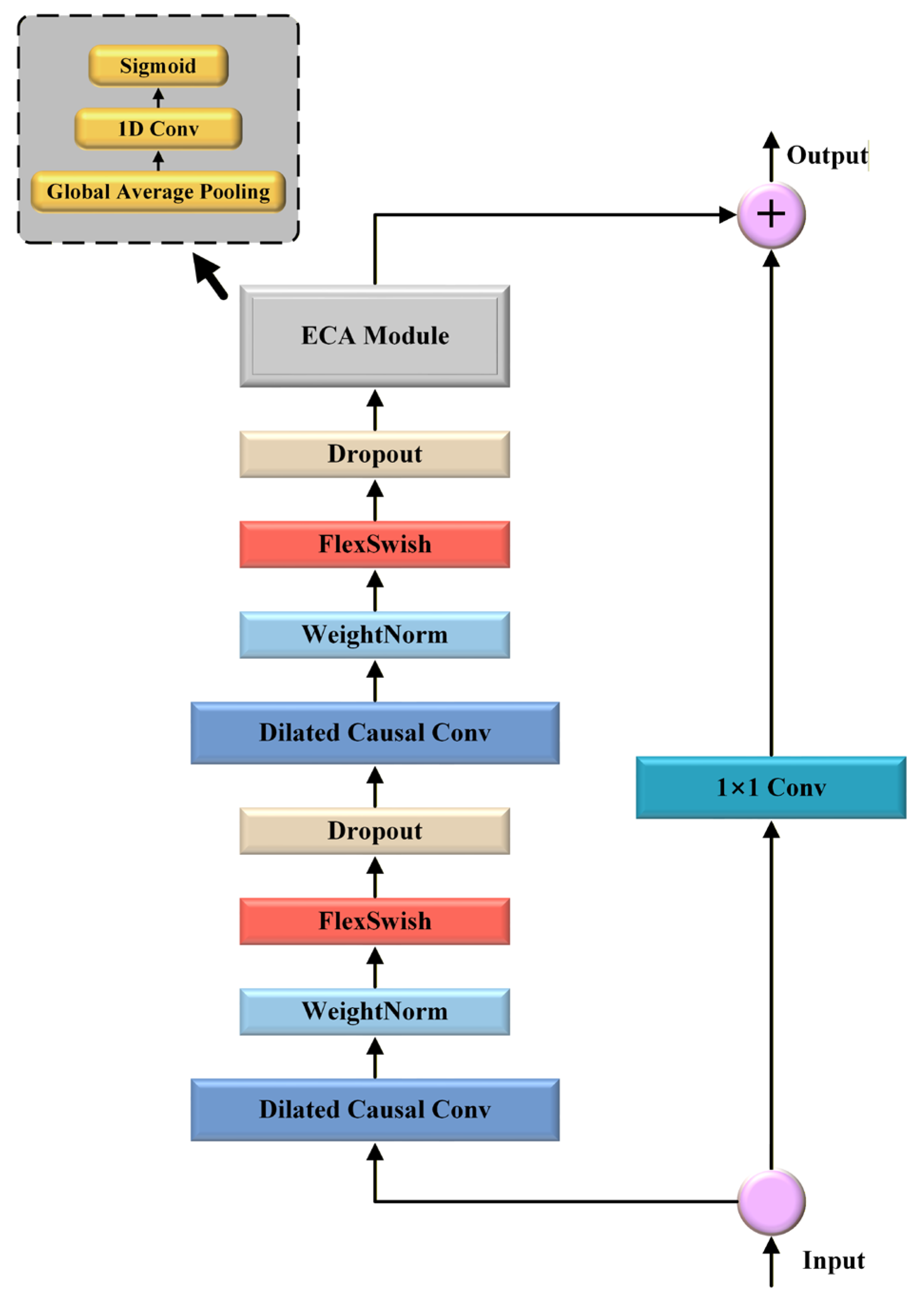
The structure of a TCN consists of residual blocks, causal dilated convolutions, weight normalization, ReLU activation functions, and dropout regularization layers. The architecture is illustrated in Figure 11. The colors in the figure are used solely for visualization purposes and do not represent any specific meaning.
This architecture alleviates the gradient explosion problem and accelerates model convergence through weight normalization. The ReLU activation function and dropout layer within the residual blocks work together to suppress overfitting and enhance the generalization capability of the network. Additionally, the residual branch applies 1 × 1 convolutions to perform nonlinear mappings for dimensional alignment, thereby ensuring consistency and information fidelity during feature fusion between the main and residual paths. However, TCN suffers from limited nonlinear expressiveness and constrained gradient propagation. To address these limitations, this paper introduces two major structural innovations based on the original TCN framework:
First, a FlexSwish activation function is proposed to replace the original ReLU. FlexSwish adaptively regulates the smoothness and the response strength in the negative domain. While maintaining linearity in the positive domain, it enables dynamic control over the response and transition smoothness of the negative domain via tunable parameters. This effectively mitigates the information truncation and gradient discontinuity issues associated with ReLU, thereby enhancing model training stability and feature representation capability.
Second, a structural optimization of the residual module is conducted to improve the model’s ability to capture temporal feature dependencies. Specifically, a lightweight Efficient Channel Attention mechanism is introduced, enabling adaptive feature weighting along the channel dimension. This enhances the global representation and feature selection capacity for time series while maintaining a compact model structure.

2.3.2. FlexSwish Activation Function

To address the issue of the ReLU activation function, which outputs zero for all negative inputs and may lead to neuron inactivation, this paper proposes an improved activation function named FlexSwish (Flexible Swish). Based on the Swish function, FlexSwish introduces three tunable parameters: m , k , and x 0 , which control the response strength for negative inputs, the steepness of the smooth transition, and the central position of activation, respectively. Its mathematical formulation is given as follows:
f ( x ) = x [ m + ( 1 m ) σ ( k ( x x 0   ) ) ]
where σ ( · ) denotes the Sigmoid function. When m = 0 and k = 1 , the FlexSwish function degenerates into the standard Swish function. This design ensures that the FlexSwish activation function is continuously differentiable over its entire domain. It retains linearity on the positive axis while enabling a smooth response on the negative axis, thereby achieving a balance between gradient propagation stability and feature representation capacity.
In the FlexSwish activation function, the parameters m and k play a critical role in model performance, particularly under scenarios with significant load fluctuations. The parameter m controls the response strength to negative inputs; smaller values of m help suppress abrupt changes in volatile regions, thereby enhancing the model’s robustness. The parameter k adjusts the smoothness of the transition, and a reduced k value allows the model to better capture subtle variations in relatively stable load patterns.
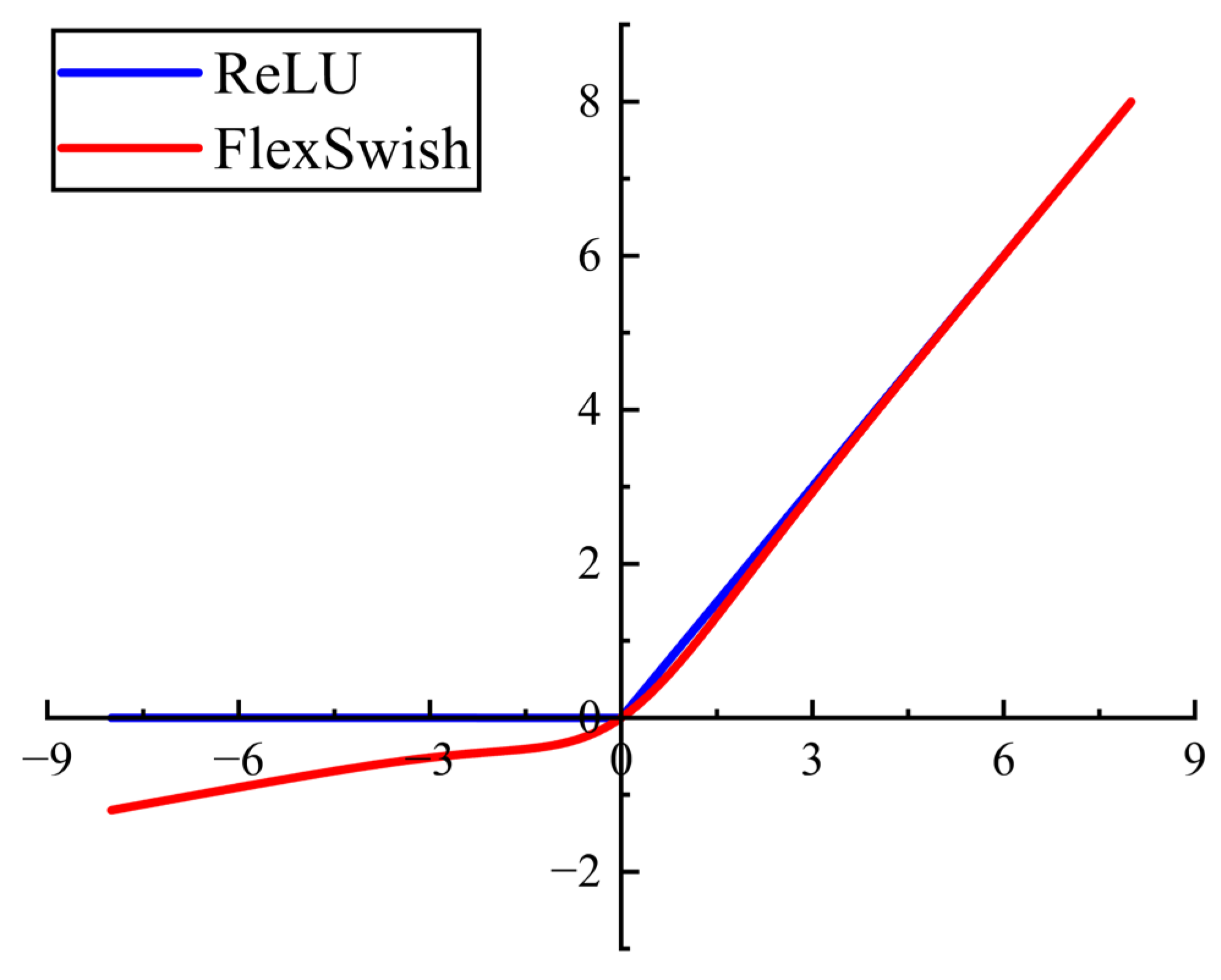
Figure 12 compares the function curves of ReLU and FlexSwish, with the blue line representing ReLU and the red line representing FlexSwish. As shown in the figure, the main advantages of FlexSwish are reflected in the following two aspects:
1.
Retention of negative-axis response and improved gradient propagation
By controlling the minimum response to negative inputs via the parameter m , FlexSwish maintains nonzero output and gradient values on the negative axis. This effectively mitigates the “dead neuron” issue commonly encountered with ReLU, as illustrated in Figure 12. This property allows deep networks to sustain more stable gradient flows during training, reduces neuron inactivation, and significantly enhances convergence efficiency and continuity in feature representation for complex temporal tasks.
2.
Smooth nonlinear transitions and preservation of linear mapping in the positive region
The parameter k adjusts the smoothness of the transition between the negative and positive regions, ensuring that the activation curve remains continuously differentiable around zero. This enables the model to adaptively capture nonlinear trends and abrupt changes in power load sequences. Moreover, FlexSwish maintains an approximately linear relationship ( f ( x ) x ) when x > 0 , thereby preserving the amplitude scaling of input features. This property is particularly important in continuous regression tasks such as load forecasting, as it helps ensure physical consistency and interpretability of the model outputs.
In summary, FlexSwish achieves a favorable balance between gradient propagation and feature expressiveness by introducing a tunable response on the negative axis while maintaining smooth continuity across the entire domain. This function not only improves the training stability of deep TCNs but also provides a more interpretable nonlinear mapping mechanism suitable for physically constrained tasks such as power load forecasting.

2.3.3. Residual Structure Enhanced with Lightweight Efficient Channel Attention

To extract multi-scale temporal dependencies, TCN leverages dilated convolutions effectively. However, the standard TCN typically applies uniform weights across all convolutional channels, neglecting the varying contributions of different feature channels to the prediction task. In the context of power load sequences, different channels often correspond to different types of temporal features, such as seasonal patterns, temperature effects, and holiday impacts. The significance of these features can vary considerably over time. If the model fails to adaptively identify and emphasize key channels, its feature representation capacity and predictive accuracy may be limited.
To address this issue, this study introduces a lightweight channel attention mechanism, known as Efficient Channel Attention, into the residual block of the TCN. The objective is to achieve adaptive weighting of feature channels, thereby enhancing the model’s responsiveness to different feature dimensions. The core idea of ECA is to capture inter-channel dependencies through a lightweight local interaction strategy and assign corresponding weights based on their importance, enabling adaptive recalibration of feature representations.
Given a convolutional output feature map X R C × T , where C is the number of channels and T denotes the temporal length, the ECA module operates as follows:
1.
Global Average Pooling (GAP)
ECA first performs global average pooling along the temporal dimension to compress each channel into a single scalar value, obtaining a global descriptor for each channel:
s c   = 1 T t = 1 T X c , t     , s = [ s 1   , s 2   , , s C   ] R C
This step compresses the two-dimensional feature map X into a one-dimensional channel vector s , where s c denotes the average response intensity of the c -th channel across the entire temporal dimension.
2.
Local Interaction Across Channels
ECA models inter-channel dependencies using one-dimensional convolution instead of fully connected layers, thereby explicitly capturing the local correlations among adjacent channels:
z = Conv 1 D ( s , k )
Here, k denotes the kernel size of the convolution, which is typically an odd number (such as 3, 5, or 7), and is used to define the range of the local receptive field. The term z represents the output obtained after applying the one-dimensional convolution.
3.
Weight Generation and Feature Recalibration
Channel-wise weights w = σ ( z ) are obtained through the Sigmoid function and then multiplied with the original feature map on a per-channel basis:
X ^ c , t = w c X c , t
Finally, the output Y is obtained through residual connection and normalization operations.
Y = LayerNorm ( X ^ + X s k i p )
The ECA module introduces a channel-level attention mechanism that effectively addresses the limitations of TCN in modeling feature importance. This design is structurally concise and efficient, allowing for explicit modeling of local channel dependencies without introducing a significant increase in the number of parameters. Its main advantages are reflected in the following three aspects:
1.
Adaptive allocation of channel weights: ECA models inter-channel dependencies through local convolution, enabling the model to automatically learn the relative contribution of different features to load variations. This mechanism enhances the response to key channels while suppressing redundant or noisy features, thereby maintaining stable feature perception during peak and mutation periods.
2.
Structural complementarity of dual-dimensional feature modeling: The introduction of ECA extends the modeling space of TCN from a single temporal dimension to a dual-dimensional structure of “temporal–channel.” While dilated convolution is responsible for hierarchical capture of temporal dependencies, ECA performs feature selection and amplification along the channel dimension. These two components complement each other in terms of information hierarchy, allowing the model to simultaneously focus on local dynamics and global patterns.
3.
Hierarchical optimization and structural synergy: ECA and FlexSwish work at different levels to jointly enhance the model’s expressive capacity. ECA operates at the channel level, optimizing the global feature distribution, whereas FlexSwish functions at the neuron level, smoothing local activations and gradient propagation. The synergy between these two mechanisms facilitates a unified and stable hierarchical system in terms of feature extraction, information flow, and computational resource allocation.
Overall, the introduction of the ECA module provides TCN with a lightweight and structurally flexible mechanism for feature regulation. The ECA module not only enhances the model’s capability for feature selection and hierarchical representation, but also offers a reliable structural foundation for multi-scale feature fusion in complex temporal tasks. The updated TCN structure is shown in Figure 13. The colors in the figure are used solely to enhance visual clarity and do not indicate any specific meaning.

2.4. Overall Model Architecture and Workflow

The model proposed in this study is named IAVOA–EATCN, which consists of the Improved African Vulture Optimization Algorithm and the Enhanced Adaptive Temporal Convolutional Network. This naming reflects the core concept of the model, namely Optimization and Model Co-Design, as well as the internal Multi-Level Adaptive Learning Mechanism. Within this framework, “EATCN” represents a structurally enhanced model built upon the standard Temporal Convolutional Network. By incorporating adaptive activation, channel recalibration, and residual enhancement mechanisms, EATCN significantly improves the nonlinear feature modeling capability and learning stability in complex load forecasting tasks.
The term “Enhanced” reflects the architectural enhancements of the model, including the Channel Feature Recalibration Module, which adaptively adjusts the contribution weights of each temporal channel feature, and the Multi-Stage Residual Structure, which strengthens information transmission and feature fidelity across convolutional layers. The term “Adaptive” indicates the model’s dynamic adjustment capabilities in both feature representation and parameter optimization. This adaptability is achieved through three interrelated mechanisms: first, the activation-level adaptive mechanism dynamically adjusts the nonlinear mapping behavior based on the distribution of input features; second, the feature-level adaptive mechanism automatically captures multi-scale temporal dependencies; and third, the optimization-level adaptive mechanism, driven by the IAVOA algorithm, dynamically balances global exploration and local exploitation during hyperparameter tuning.
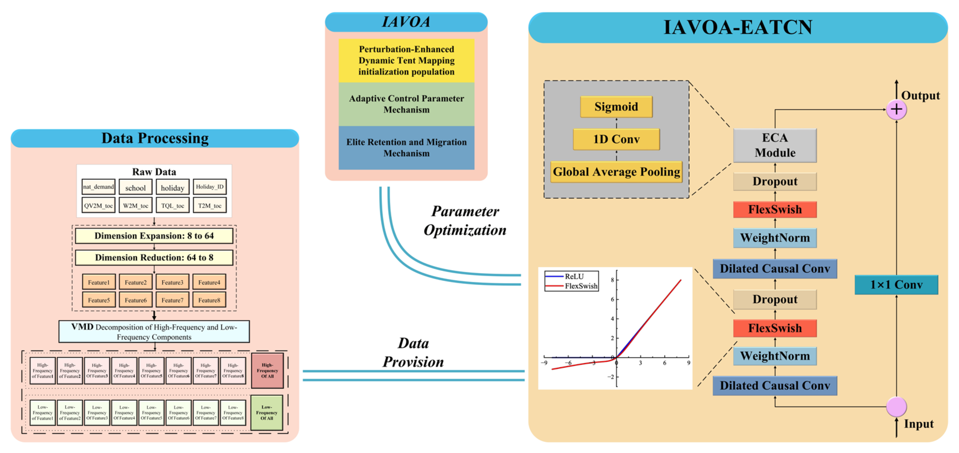
Figure 14 illustrates the overall construction workflow of the proposed model. The different colors in the figure are used solely for visual enhancement and do not carry any specific meaning. The overall structure is divided into two main modules: Data Processing and Forecast Modeling (IAVOA-EATCN). The advantages of this feature engineering framework are summarized as follows:
  • Strong information preservation capability: The dimensional expansion–reduction process effectively retains important hidden information from weakly correlated features that may influence load variation.
  • High decomposition efficiency: The VMD algorithm is easy to implement and computationally efficient, reducing model complexity while maintaining high decomposition quality.
  • Strong methodological generality: This feature engineering framework is not only applicable to the dataset used in this study, but also generalizable to other forecasting scenarios involving multi-feature inputs, providing a reference for future feature engineering designs.
In the modeling and optimization part, the proposed IAVOA-EATCN model introduces several key improvements based on the TCN structure and AVOA algorithm. The advantages are summarized as follows:
  • Introduction of the FlexSwish activation function: This function is an improved version of the Swish activation, which retains the negative value region and introduces tunable parameters for enhanced nonlinear expressiveness. Experiments verify that it significantly improves prediction accuracy.
  • Synergistic integration of ECA attention mechanism and TCN: ECA extends the temporal dimension to a “temporal–channel” dual-dimensional structure and adaptively emphasizes key channel features, enabling the model to focus on both local dynamics and global patterns at different scales. The integration scheme developed in this paper provides a valuable reference for combining attention mechanisms with temporal convolutional models.
  • Performance enhancement of the AVOA algorithm: To address limitations in the original AVOA, three improvement strategies are proposed: a perturbation-based dynamic Tent map initialization, an adaptive control parameter mechanism, and an elite preservation–migration mechanism. Experimental results demonstrate that these enhancements significantly improve optimization efficiency and convergence stability. These strategies also offer practical insights for dynamic regulation and structural optimization of other swarm intelligence algorithms.
Algorithm 1 shows the pseudocode of the IAVOA–EATCN method. The pseudocode systematically describes the key steps of the algorithm, including feature engineering, model construction, and prediction output. This formal representation clearly presents the structure and operations of the algorithm, simplifying the understanding of complex steps and enhancing the readability of the algorithm.
Algorithm 1: IAVOA–EATCN-based Load Forecasting Framework
Input:
Original   multivariate   load   dataset   X = x 1 , x 2 , x 3 , , x n
Output:
  Predicted load sequence Y
/* Feature Engineering */
1 : Perform   dimensional   expansion   on   X   to   obtain   high-dimensional   features   X 64
2 :   Apply   dimensional   reduction   on   X 64   to   obtain   reconstructed   features   X 8
3 :   Decompose   X 8 using Variational Mode Decomposition
4 :   Extract   low-frequency   component   X L o w   and   high-frequency   component   X H i g h
5 :   Construct   final   feature   set   X i n = L o a d , T e m p e r a t u r e ,   X L o w ,   X H i g h
/* Model Construction */
6: Initialize Temporal Convolutional Network
7: Replace original activation function with FlexSwish
8: Embed Efficient Channel Attention module into TCN
9: Construct the EATCN prediction model
/* Hyperparameter Optimization */
10: Initialize population using Perturbation-Enhanced Dynamic Tent Mapping
11: For each iteration do
12:    Evaluate fitness of each individual using prediction error
13:    Update population using adaptive exploration–exploitation strategy
14:    Apply elite retention and migration mechanism
15: End for
16: Obtain optimal hyperparameters θ
17: Train EATCN using optimized hyperparameters θ on Xin
18: Generate predicted load Y ^
19: Return Y ^

3. Results

To evaluate the performance of the proposed IAVOA-EATCN model in power load forecasting, this study designs three experimental components: benchmark model selection, comparison of model improvement effects, and performance enhancement of the optimization algorithm. The dataset used in the experiments is derived from the power load data that has undergone the feature engineering process described earlier. In the benchmark model selection phase, several representative RNN-based architectures are compared, including LSTM, GRU, BiLSTM, and BiGRU. Additionally, the widely adopted Transformer model is also included in the comparison. For the model improvement analysis, a series of ablation experiments are conducted to progressively verify the individual contribution of each enhancement module to the performance of the baseline TCN model. It is worth noting that all experiments are conducted using the feature-engineered dataset mentioned above. Before being fed into the model, all input data are normalized, and the outputs are subsequently denormalized to restore the original scale. Finally, the study compares the application performance of different optimization algorithms on the EATCN model. The experimental results demonstrate that the proposed IAVOA algorithm can significantly enhance the forecasting performance of the model.

3.1. Baseline Model Performance Comparison Experiment

During the baseline model selection stage, comparative experiments were conducted on representative models from RNN-based, CNN-based, and encoder-decoder architectures. By evaluating the performance of each model on the same dataset and visualizing the trends of their prediction results, the differences between predicted outputs and actual load variations can be intuitively observed. These visualizations help reveal the strengths and weaknesses of each model in capturing load variation trends, thereby providing a reference for subsequent model optimization. In addition, multiple evaluation metrics were employed to quantitatively assess the prediction results of each model. This approach enables a clear mathematical comparison of the models’ predictive performance, ensuring the systematicity and objectivity of the evaluation process. The corresponding experimental results are shown in Figure 15 and Figure 16, and Table 6.
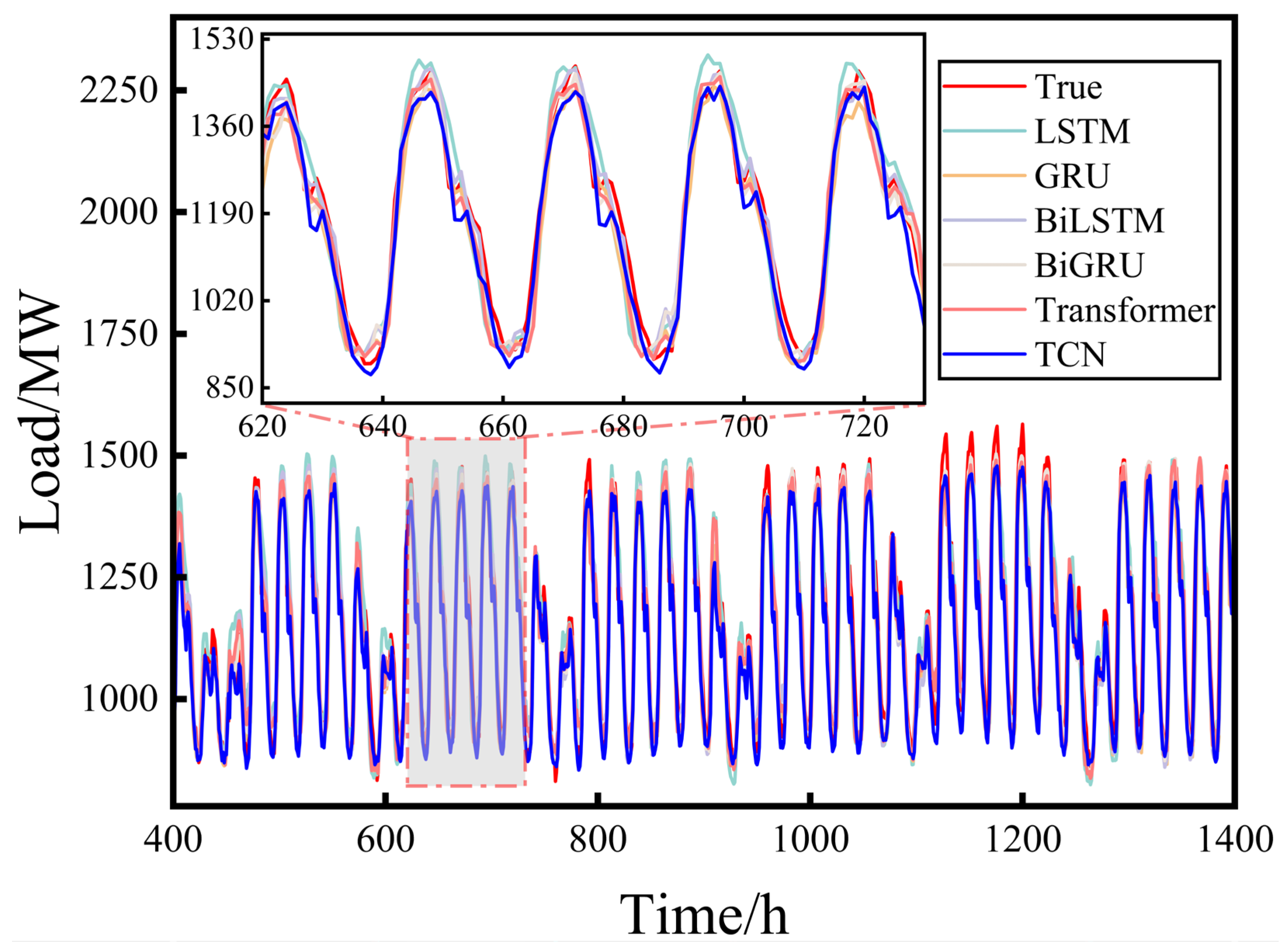
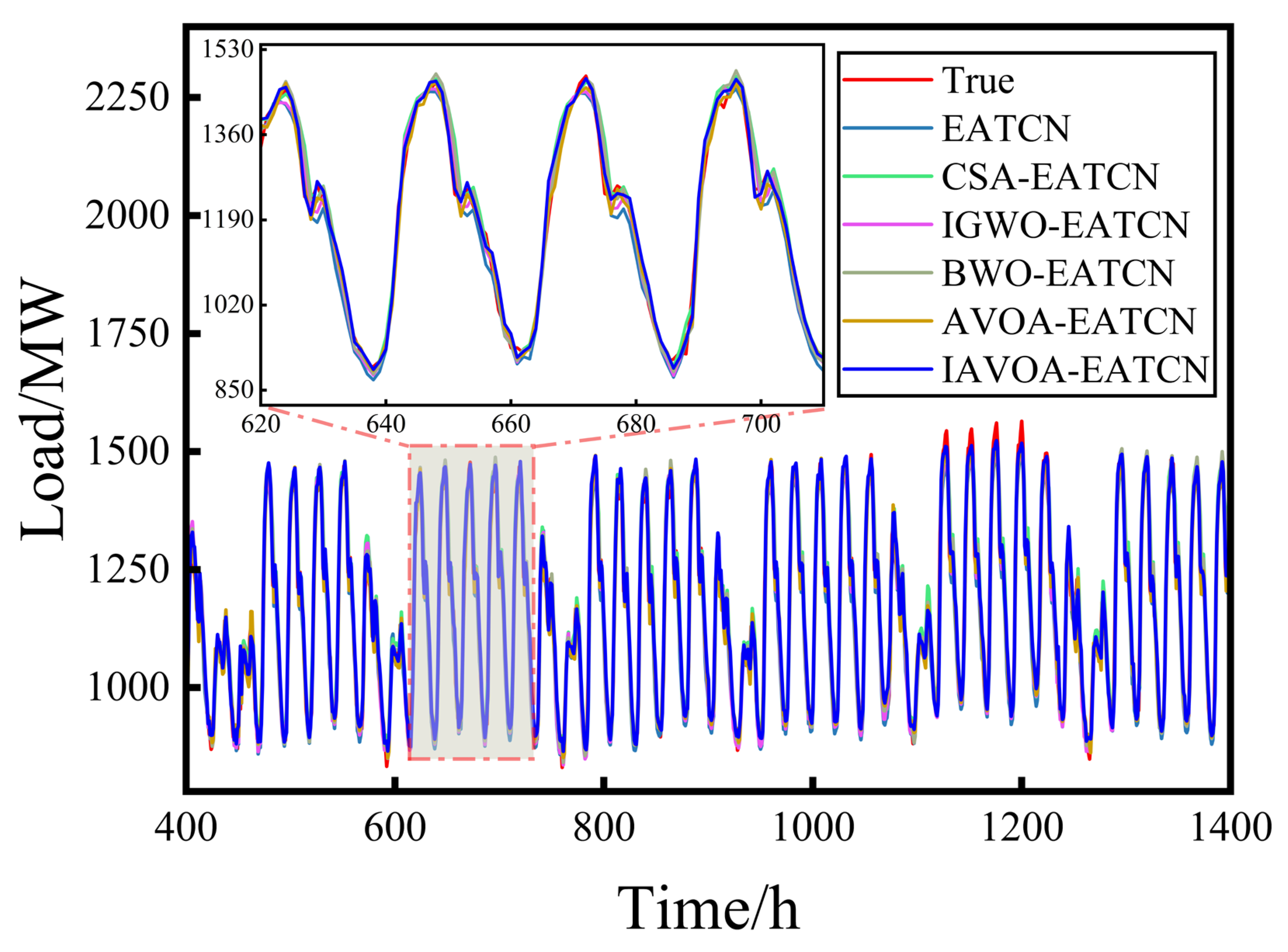
Figure 15 illustrates the fitting performance of six selected models in the task of power load forecasting. The horizontal axis represents time in hours, while the vertical axis denotes load values in megawatts (MW). To facilitate a more intuitive comparison of model performance, a local magnified view is included within the figure, using the same axes as the main plot. The red curve represents the actual load values, while the curves in other colors indicate the prediction results of different models. The specific color used for each model is clearly labeled in the figure.
As shown in the figure, all models are capable of capturing the periodic variation patterns of the load values, demonstrating a certain level of time series modeling capability. The local magnified view presents more clearly the performance differences among models during periods of large fluctuations, which helps in more accurately evaluating the fitting precision. The experimental results indicate that the prediction curve of the TCN model closely aligns with the actual curve, showing minimal error and effectively capturing the peaks and valleys in a timely manner. When the load sequence exhibits significant fluctuations, the TCN model maintains a stable prediction trend, reflecting its strong robustness. This stability stems from the unique advantages of the TCN model, which processes multi-scale temporal information through convolutional operations, enabling it to effectively capture both long-term dependencies and local patterns, thereby maintaining high prediction accuracy under complex load variation conditions.
In contrast, RNN-based models exhibit considerable fluctuation at the peaks and troughs, mainly due to their susceptibility to gradient vanishing or explosion when handling long sequences, which limits their ability to capture long-term dependencies. Unlike these models, the CNN-based TCN effectively alleviates gradient-related issues through convolution and causal convolution structures, while significantly improving training efficiency and prediction accuracy through parallel computation.
In addition, the Transformer model, which is based on an encoder-decoder structure, also demonstrates relatively stable prediction performance, as it is likewise derived from CNN architectures and employs self-attention mechanisms to capture long-range dependencies within the sequence. However, the Transformer model is structurally more complex, and its dual-layer encoder-decoder framework demands higher computational resources, resulting in longer training and inference times. Considering the limitations of the experimental hardware and the need for efficient prediction, the TCN model was ultimately selected as the baseline model under the same experimental conditions due to its faster execution speed, simpler architecture, and higher accuracy.
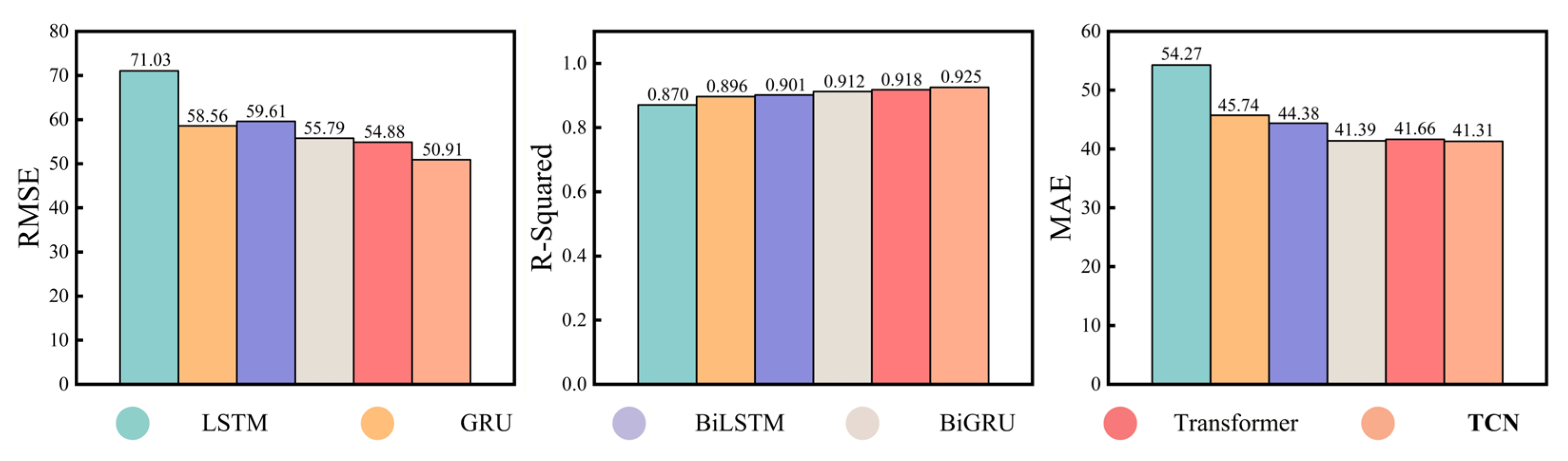
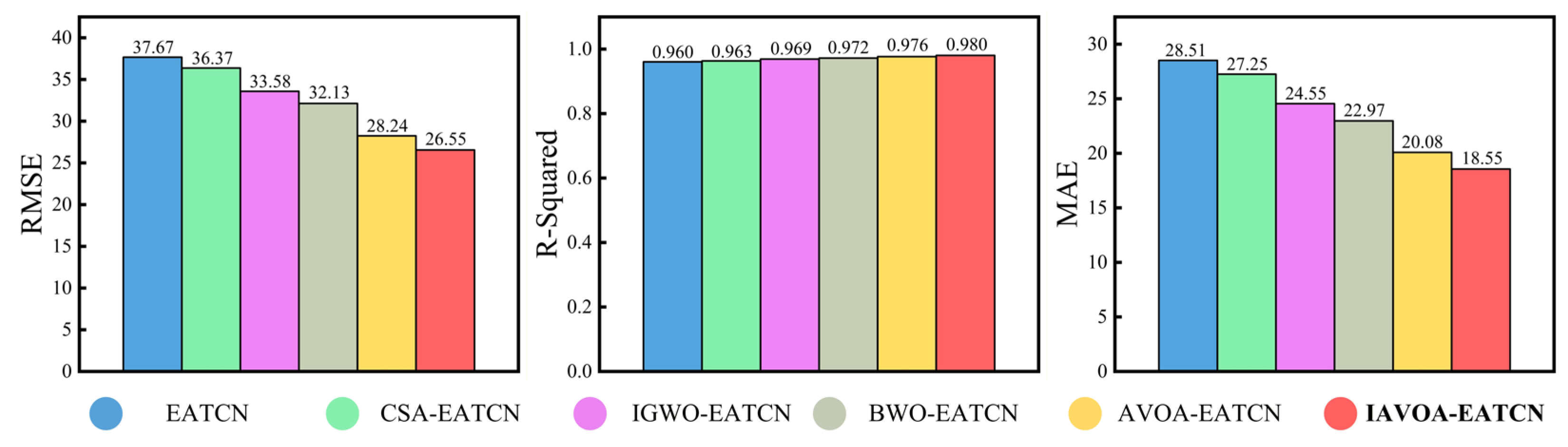
Figure 16 presents the performance of each baseline model under three evaluation metrics. The legend indicates the prediction models corresponding to different colors, while the vertical axis represents the numerical values of the evaluation metrics. By using bar charts, the prediction performance of different models under each metric can be compared more intuitively.
Based on the results presented in Figure 16 and Table 6, the TCN model demonstrates outstanding performance across all evaluation metrics. Its RMSE value is 50.9168, which is significantly lower than those of other models, indicating the smallest prediction error. In terms of the R2 metric, the TCN achieves a high score of 0.9256, outperforming the other baseline models and highlighting its excellent fitting capability. Although the differences in MAE values among the models are relatively small, the TCN still maintains the lowest value.
Although RNN-based models, especially those with gating mechanisms such as LSTM, GRU, and their bidirectional variants, have certain advantages in modeling short-term dependencies and are suitable for relatively stable time series data, they fail to respond effectively to sudden load changes in the dataset used in this study, resulting in relatively large prediction errors. These models do not demonstrate clear predictive advantages when dealing with complex dynamic variations such as load fluctuations.

3.2. Validation Experiments for EATCN

To validate the effectiveness of the improvements introduced in the proposed EATCN model, a series of ablation experiments were conducted. By progressively incorporating different enhancement modules, the impact of each modification on the performance of the base model was evaluated. Additionally, the predicted results were visualized to analyze the specific contribution of each component to the improvement in prediction performance. Specifically, this study compares the original TCN, the TCN with the improved activation function FlexSwish, the TCN incorporating the lightweight channel attention mechanism, and the final proposed EATCN model. The FlexSwish function is configured with parameters m = 0 and k = 0.9 . The corresponding experimental results are shown in Figure 17 and Figure 18, and Table 7.
Figure 17 illustrates the model fitting results after progressively incorporating different enhancement modules under the same dataset. As shown in the figure, based on the already strong predictive performance of the original TCN, the application of these improvements significantly enhances the overall model performance. After replacing the activation function with FlexSwish, the TCN demonstrates a more sensitive response to sudden changes in load. Compared with the original TCN, which tends to respond more smoothly during abrupt fluctuations, the inclusion of the FlexSwish activation function enables the model to capture load variations more accurately. Specifically, the original TCN often underestimates the load during rapid transitions due to its inherent stability, while the modified version with FlexSwish produces significantly improved predictions. This improvement mainly stems from the ability of FlexSwish to retain negative values, thus avoiding the limitation of ReLU, which sets all negative values to zero. Unlike ReLU, which discards negative information, FlexSwish preserves it, thereby maintaining memory-related information within the model and enabling the network to respond more sensitively and accurately to sharp fluctuations. This, in turn, enhances the overall prediction accuracy and robustness.
By comparing the predictive results of the TCN integrated with the ECA mechanism to those of the original TCN, it is evident that the introduction of the lightweight channel attention mechanism significantly improves the predictive accuracy. The proposed EATCN model combines the advantages of the FlexSwish activation function, notably improving response accuracy during load mutations, and integrates the lightweight channel attention mechanism to further strengthen its focus on critical information. Its fitted curve aligns closely with the actual values, especially in regions of load fluctuation, where it exhibits smoother and more precise responses. This demonstrates superior trend-tracking capability and prediction accuracy. Notably, the FlexSwish activation function designed in this study features tunable parameters, allowing for flexible configuration tailored to specific tasks. This adaptability enhances the model’s robustness and performance across diverse load forecasting scenarios.
According to the results presented in Figure 18 and Table 7, it is evident that the predictive performance of the original TCN model has been significantly improved after incorporating different enhancement modules. The introduction of the FlexSwish activation function notably improved the model’s prediction accuracy, reducing the RMSE from 55.7958 to 48.2997 and increasing the R2 from 0.9256 to 0.9319. This indicates that FlexSwish enhances the model’s ability to capture variations in power load by strengthening the nonlinear expressive capacity of the activation function.
On the other hand, introducing the ECA module into the TCN alone led to a notable performance improvement compared to the original TCN. Specifically, the RMSE decreased from 55.7958 to 40.6956, the R2 score increased from 0.9256 to 0.9533, and the MAE dropped from 41.3957 to 30.7077. These results indicate that the ECA module significantly enhances the model’s predictive accuracy and reduces forecasting errors. By adaptively adjusting channel-wise weights, ECA enables the model to focus more on critical features and automatically optimize the contribution of each channel, thereby improving its ability to capture complex data patterns and enhancing overall prediction performance.
Finally, the EATCN model, which integrates both FlexSwish and ECA, achieved the best performance across all evaluation metrics. The RMSE was reduced to 37.6712, the R2 improved to 0.9607, and the MAE decreased to 28.5131. The synergistic effect of FlexSwish and ECA optimized the training process and substantially improved the prediction accuracy, validating the critical role of their integration in enhancing power load forecasting performance.

3.3. Validation Experiments for Optimization Algorithm Performance

To further enhance the predictive performance of the EATCN model, this study introduces several intelligent optimization algorithms aimed at automatically tuning critical hyperparameters such as the number of hidden units, batch size, and learning rate, without significantly increasing the model’s complexity. Specifically, the performance improvement of the EATCN model is evaluated under five optimization algorithms: CSA, IGWO, BWO, AVOA, and IAVOA. All experiments were performed using identical hyperparameter settings and stopping conditions. By comprehensively assessing each algorithm’s performance in terms of prediction error and fitting accuracy, this study provides an in-depth analysis of their practical effectiveness in complex load forecasting tasks.
As shown in Figure 19, the EATCN model optimized with different algorithms exhibits varying degrees of improvement in fitting accuracy and prediction consistency, with the most notable enhancement observed under the IAVOA optimization. The zoomed-in section clearly demonstrates that the predicted results closely match the actual values at both the peaks and troughs of the load curve, indicating that the predictive accuracy of the model has been significantly improved after hyperparameter tuning via the optimization algorithm. When the load values fluctuate sharply, the optimized model responds quickly to the changes while maintaining low prediction error, thereby enhancing both prediction accuracy and response speed.
Compared to the original, non-optimized EATCN model, all optimization algorithms contribute to performance improvements despite the presence of some prediction errors. The integration of optimization algorithms not only strengthens the model’s learning capability without substantially increasing its complexity but also enhances predictive accuracy under limited computational resources. This effectively maximizes the model’s potential and improves its overall performance.
As shown in the bar chart in Figure 20 and the evaluation metrics presented in Table 8, integrating different optimization algorithms with the prediction model led to varying degrees of performance improvement. Among them, the improved IAVOA demonstrated the most significant enhancement and achieved the best results across all evaluation metrics. Specifically, its RMSE decreased to 26.5544, indicating that the optimization algorithm effectively reduced prediction error and improved forecasting accuracy. The R2 value exceeded 0.98, representing a substantial improvement over other optimization algorithms and highlighting the enhanced fitting capability of the model. Moreover, its MAE dropped below 20, reaching 18.5589, demonstrating that the IAVOA-based optimization resulted in a more stable model for load forecasting.
In detail, the RMSE of the BWO-EATCN model decreased by 5.5401 (from 37.6712 to 32.1311), and the MAE decreased by 5.5415 compared to the original EATCN, indicating that this optimization algorithm has a strong advantage in error control. The RMSE of the AVOA-EATCN model further dropped to 28.2444, a reduction of 9.4268 from the original model, and its MAE decreased to 20.0855, confirming the enhancement in modeling load fluctuations. The improved IAVOA-EATCN model outperformed all others across the evaluation metrics, fully demonstrating the effectiveness of the proposed optimization strategy in improving prediction accuracy and model stability.
Overall, the experimental results confirm that the IAVOA optimization algorithm significantly enhances the performance of the EATCN model. The optimized IAVOA-EATCN model achieved the best performance in multiple evaluation metrics, particularly excelling in error control, trend tracking, and load fluctuation response. The integration of this optimization algorithm with a deep prediction model has proven its effectiveness in power load forecasting tasks, providing a reliable solution for improving both predictive accuracy and model robustness.

3.4. Comparative Analysis of Prediction Accuracy and Resource Usage

To comprehensively evaluate the practical performance of each model, this section conducts a comparative analysis from two perspectives: prediction accuracy and computational resource consumption. By highlighting the trade-off between accuracy and efficiency, the analysis provides a valuable reference for model selection and deployment in various application scenarios. Table 9 summarizes the performance of each model across evaluation metrics, where time is measured in seconds and memory usage in megabytes (MB), allowing for a clear and comprehensive comparison.
As shown in Table 9, both prediction accuracy and computational efficiency improve significantly with model enhancements. The baseline TCN model achieves an RMSE of 55.7958 and an R2 of 0.9256, reflecting moderate performance. FlexSwish+TCN, with an improved activation function, reduces the RMSE to 48.2997 and slightly increases the R2 to 0.9319, while keeping training time and memory consumption nearly unchanged compared to the original TCN. After incorporating the ECA module, the ECA+TCN model achieves a much lower RMSE of 40.6956 and a higher R2 of 0.9533; however, training time increases to 697.4 s and memory usage rises to 357.9 MB.
The final EATCN model, which combines the adaptive activation function and ECA module, further improves prediction accuracy with an RMSE of 37.6712 and an R2 of 0.9607, achieving the best performance among the unoptimized models. Although the training time (713.6 s) and memory usage (360.1 MB) slightly increase, the overall performance is superior.
After introducing the optimization algorithm, the IAVOA-EATCN model exhibits the most outstanding performance. It achieves an RMSE of 26.5544, an R2 of 0.9804, and an MAE of 18.5589, indicating a significant improvement in prediction accuracy. Although the training time increases to 873.5 s compared to EATCN, this is considered an acceptable trade-off given the accuracy gains. Memory usage rises to 429.2 MB, slightly higher than the 360.1 MB of EATCN, but the increase is relatively modest. Compared with other optimization algorithm-based models, IAVOA-EATCN demonstrates more efficient resource usage and superior accuracy, offering an ideal balance between computational cost and predictive performance. Therefore, IAVOA-EATCN is undoubtedly the most effective model presented, making it well-suited for scenarios that require high accuracy with reasonable computational overhead.

4. Conclusions

With the development of power systems toward large-scale and intelligent operations, the importance of load forecasting in ensuring supply-demand balance and maintaining system stability has become increasingly prominent. Meanwhile, in the design of power system topology and dispatch mechanisms, strategies such as regional symmetry, structural mirroring, and operational balance are commonly adopted to simplify scheduling control and enhance system redundancy and stability. This type of structural symmetry is reflected in various stages of power generation, transmission, and distribution, which leads to certain symmetrical characteristics in the spatial distribution of loads and dispatching behaviors.
To address these challenges, this paper proposes a novel feature engineering method aimed at enhancing the model’s ability to represent and learn from complex load data. First, a dimensionality enhancement–reduction strategy is applied to reconstruct the original features, which helps introduce potential higher-order interactions and improve the efficiency of subsequent modeling. Then, Variational Mode Decomposition is applied to the reduced-dimension key features to enhance the model’s sensitivity to load components at different frequency levels. As a result of this preprocessing, the dimensionality of the input features is reduced by approximately 50% compared to the original data, significantly lowering computational complexity while preserving the main structural relationships between features and improving the model’s capability for time-frequency decomposition of load patterns. This feature engineering approach provides a feasible and effective pathway for load forecasting tasks involving high-dimensional, multi-feature inputs. Experimental results have confirmed its advantages in both prediction accuracy and computational efficiency.
In terms of model architecture, this study addresses the limited information retention capability of conventional activation functions in the original Temporal Convolutional Network by designing and introducing the FlexSwish activation function. Compared with ReLU, FlexSwish retains negative value information, thereby improving the continuity and nonlinear representation capability of features, particularly in the context of modeling sudden load changes. In addition, an Efficient Channel Attention mechanism is integrated into the model to enable adaptive weighting of key feature channels, enhancing the model’s ability to focus on informative inputs. The attention mechanism complements the multi-scale temporal features extracted by dilated convolutions at different hierarchical levels. Through this symmetric structural design, the model is able to attend simultaneously to local dynamic details and global trend patterns, thereby increasing the depth and breadth of load pattern modeling.
In terms of parameter optimization, the improved African Vulture Optimization Algorithm proposed in this paper incorporates three key mechanisms. The Perturbation-Enhanced Dynamic Tent Mapping improves the diversity and distribution balance of population initialization. The Adaptive Parameter Control mechanism enables dynamic adjustment between exploration and exploitation during the search process. The Elite Retention and Migration mechanism ensures the sustained utilization of high-quality solutions and maintains population vitality. These optimization strategies effectively overcome the limitations of the original AVOA, such as premature convergence and slow search speed, and significantly improve the stability and global search capability of the model during hyperparameter optimization.
Experimental results demonstrate that the proposed model outperforms the benchmark methods across multiple evaluation metrics, leading to the following major conclusions:
  • Performing dimensionality expansion and reduction on the original data facilitates the discovery of potential high-order feature interactions. When combined with signal decomposition techniques, this approach can significantly reduce feature dimensionality, thereby enhancing the model’s ability to represent complex load patterns and improving computational efficiency while preserving essential information.
  • The dilated convolution in the TCN framework provides advantages in expanding the receptive field and capturing long-term dependencies. Based on this, the integration of the Efficient Channel Attention mechanism further enhances the model’s ability to selectively focus on key feature channels, thereby improving feature representation and modeling accuracy in load forecasting tasks.
  • Through systematic improvements in feature engineering, model architecture, and optimization strategy, the proposed IAVOA-EATCN model has achieved significant performance gains in load forecasting. Experimental results show that the model reaches an RMSE of 26.5544, an R2 of 0.9804, and an MAE of 18.5589, outperforming the baseline TCN model in both predictive accuracy and fitting capability.
In summary, this study proposes a deep forecasting model, IAVOA-EATCN, which integrates an improved African Vulture Optimization Algorithm. In the feature engineering stage, the model effectively improves the utilization efficiency of feature information. In terms of model structure, the incorporation of the FlexSwish activation function and the ECA attention mechanism significantly enhances the model’s feature representation capability. Regarding the optimization strategy, the improved IAVOA algorithm demonstrates superior search performance across multiple objective functions. In addition, IAVOA-EATCN adopts an offline training and prediction mode, and introduces an error-threshold-triggered mechanism and a periodic update strategy during deployment.
Specifically, when the prediction error consistently exceeds a predefined threshold, the system automatically prompts model retraining to adapt to potential changes in data distribution. Meanwhile, the model is also periodically retrained in offline mode to ensure long-term forecasting stability and adaptability. This mechanism enables the model to maintain high performance in dynamic application environments without the need for continuous manual intervention. Comprehensive experimental results demonstrate that IAVOA-EATCN achieves a simplified architecture, high prediction accuracy, and strong generalization ability in short-term power load forecasting tasks, providing both theoretical and practical support for relevant engineering applications.

Author Contributions

Conceptualization, Z.P.; methodology, H.H.; software, J.M.; validation, Z.P. and H.H.; formal analysis, Z.P.; data curation, J.M.; writing—original draft preparation, Z.P.; writing—review and editing, Z.P. and H.H.; visualization, J.M. and H.H.; supervision, Z.P. All authors have read and agreed to the published version of the manuscript.

Funding

This research received no external funding.

Data Availability Statement

The dataset utilized in this study is publicly accessible and can be retrieved from the Kaggle platform at the following link: https://www.kaggle.com/datasets/saurabhshahane/electricity-load-forecasting, accessed on 10 October 2025.

Conflicts of Interest

The authors declare no conflicts of interest.

References

  1. Massaoudi, M.; Abu-Rub, H.; Refaat, S.S.; Chihi, I.; Oueslati, F.S. Deep learning in smart grid technology: A review of recent advancements and future prospects. IEEE Access 2021, 9, 54558–54578. [Google Scholar] [CrossRef] [Scilit]
  2. Shahriar, S.; Al-Ali, A.-R.; Osman, A.H.; Dhou, S.; Nijim, M. Prediction of EV charging behavior using machine learning. IEEE Access 2021, 9, 111576–111586. [Google Scholar] [CrossRef] [Scilit]
  3. Karamolegkos, S.; Koulouriotis, D.E. Advancing short-term load forecasting with decomposed Fourier ARIMA: A case study on the Greek energy market. Energy 2025, 325, 135854. [Google Scholar] [CrossRef] [Scilit]
  4. Cortes, C.; Vapnik, V. Support-vector networks. Mach. Learn. 1995, 20, 273–297. [Google Scholar] [CrossRef] [Scilit] [PubMed]
  5. Breiman, L. Random forests. Mach. Learn. 2001, 45, 5–32. [Google Scholar] [CrossRef] [Scilit]
  6. Chen, T. XGBoost: A Scalable Tree Boosting System. In Proceedings of the 22nd ACM SIGKDD International Conference on Knowledge Discovery and Data Mining, San Francisco, CA, USA, 13–17 August 2016; Cornell University: Ithaca, NY, USA, 2016. [Google Scholar] [CrossRef] [Scilit]
  7. Graves, A. Long short-term memory. In Supervised Sequence Labelling with Recurrent Neural Networks; Springer: Berlin/Heidelberg, Germany, 2012; pp. 37–45. [Google Scholar] [CrossRef] [Scilit]
  8. Graves, A.; Schmidhuber, J. Framewise phoneme classification with bidirectional LSTM and other neural network architectures. Neural Netw. 2005, 18, 602–610. [Google Scholar] [CrossRef] [Scilit]
  9. LeCun, Y.; Bengio, Y.; Hinton, G. Deep learning. Nature 2015, 521, 436–444. [Google Scholar] [CrossRef] [Scilit] [PubMed]
  10. Katholnigg, M.; Goebel, C. The Impact of Load Forecasting Model Choice on the Economic Operation of Industrial Energy Storage. In Proceedings of the 12th ACM International Conference on Systems for Energy-Efficient Buildings, Cities, and Transportation, Golden, CO, USA, 19–21 November 2025; pp. 12–22. [Google Scholar] [CrossRef] [Scilit]
  11. Gao, S.; Xiang, C.; Zhou, Y.; Liu, H.; Dai, L.; Zhang, T.; Yin, Y. A Hybrid Model Combining Signal Decomposition and Inverted Transformer for Accurate Power Transformer Load Prediction. Appl. Sci. 2025, 15, 11241. [Google Scholar] [CrossRef] [Scilit]
  12. Han, H.; Peng, J.; Ma, J.; Liu, H.; Liu, S. Research on Load Forecasting Prediction Model Based on Modified Sand Cat Swarm Optimization and SelfAttention TCN. Symmetry 2025, 17, 1270. [Google Scholar] [CrossRef] [Scilit]
  13. Han, H.; Peng, J.; Ma, J.; Liu, S.L.; Liu, H. Research on load forecasting based on CEEMDAN SE VMD and SelfAttention TCN fusion model. Sci. Rep. 2025, 15, 14530. [Google Scholar] [CrossRef] [Scilit]
  14. Ma, J.; Peng, J.; Han, H.; Song, L.; Liu, H. A hybrid power load forecasting model using BiStacking and TCN-GRU. PLoS ONE 2025, 20, e0321529. [Google Scholar] [CrossRef] [Scilit]
  15. Abdollahzadeh, B.; Gharehchopogh, F.S.; Mirjalili, S. African vultures optimization algorithm: A new nature-inspired metaheuristic algorithm for global optimization problems. Comput. Ind. Eng. 2021, 158, 107408. [Google Scholar] [CrossRef] [Scilit]
  16. Haq, M.R.; Ni, Z. A new hybrid model for short-term electricity load forecasting. IEEE Access 2019, 7, 125413–125423. [Google Scholar] [CrossRef] [Scilit]
  17. Liu, H.; Xiong, X.; Yang, B.; Cheng, Z.; Shao, K.; Tolba, A. A power load forecasting method based on intelligent data analysis. Electronics 2023, 12, 3441. [Google Scholar] [CrossRef] [Scilit]
  18. Shi, J.; Teh, J.; Alharbi, B.; Lai, C.-M. Load forecasting for regional integrated energy system based on two-phase decomposition and mixture prediction model. Energy 2024, 297, 131236. [Google Scholar] [CrossRef] [Scilit]
  19. Chen, J.; Liu, L.; Guo, K.; Liu, S.; He, D. Short-term electricity load forecasting based on improved data decomposition and hybrid deep-learning models. Appl. Sci. 2024, 14, 5966. [Google Scholar] [CrossRef] [Scilit]
  20. Pham, Q.-V.; Mirjalili, S.; Kumar, N.; Alazab, M.; Hwang, W.-J. Whale optimization algorithm with applications to resource allocation in wireless networks. IEEE Trans. Veh. Technol. 2020, 69, 4285–4297. [Google Scholar] [CrossRef] [Scilit]
  21. Mirjalili, S.; Mirjalili, S.M.; Hatamlou, A. Multi-verse optimizer: A nature-inspired algorithm for global optimization. Neural Comput. Appl. 2016, 27, 495–513. [Google Scholar] [CrossRef] [Scilit]
  22. Braik, M.S. Chameleon Swarm Algorithm: A bio-inspired optimizer for solving engineering design problems. Expert Syst. Appl. 2021, 174, 114685. [Google Scholar] [CrossRef] [Scilit]
  23. Nadimi-Shahraki, M.H.; Taghian, S.; Mirjalili, S. An improved grey wolf optimizer for solving engineering problems. Expert Syst. Appl. 2021, 166, 113917. [Google Scholar] [CrossRef] [Scilit]
  24. Zhong, C.; Li, G.; Meng, Z. Beluga whale optimization: A novel nature-inspired metaheuristic algorithm. Knowl.-Based Syst. 2022, 251, 109215. [Google Scholar] [CrossRef] [Scilit]
Figure 1. Flowchart of Feature Engineering Process.
Symmetry 18 00102 g001
Figure 2. Pearson correlation calculation results.
Symmetry 18 00102 g002
Figure 3. Performance Comparison of Raw Data and Feature Engineered Data on Base Models.
Symmetry 18 00102 g003
Figure 4. Random Initialization of Population.
Symmetry 18 00102 g004
Figure 5. PDTM Initialization of Population.
Symmetry 18 00102 g005
Figure 6. Flowchart of IAVOA.
Symmetry 18 00102 g006
Figure 7. Schwefel’s Problem 2.21 Test Function.
Symmetry 18 00102 g007
Figure 8. Generalized Penalized Function Test Function.
Symmetry 18 00102 g008
Figure 9. Performance of different optimization algorithms on test functions. (a) Performance of Optimization Algorithms on F1(x); (b) Performance of Optimization Algorithms on F2(x).
Symmetry 18 00102 g009
Figure 10. Dilated Convolution.
Symmetry 18 00102 g010
Figure 11. The Architectural Design of TCN.
Symmetry 18 00102 g011
Figure 12. Comparison of ReLU and FlexSwish Activation Functions.
Symmetry 18 00102 g012
Figure 13. Architecture of the EATCN Model.
Symmetry 18 00102 g013
Figure 14. Overall Framework and Workflow.
Symmetry 18 00102 g014
Figure 15. Comparison of Fitting Results of Baseline Models.
Symmetry 18 00102 g015
Figure 16. Comparison of Evaluation Metric Results for Baseline Models.
Symmetry 18 00102 g016
Figure 17. Comparison of Fitting Results from Ablation Experiments on EATCN Modules.
Symmetry 18 00102 g017
Figure 18. Evaluation Metrics Comparison for Ablation Studies on EATCN Modules.
Symmetry 18 00102 g018
Figure 19. Comparison of Fitting Performance of EATCN Enhanced by Different Optimization Algorithms.
Symmetry 18 00102 g019
Figure 20. Comparison of Prediction Performance Metrics of Models Enhanced by Different Optimization Algorithms.
Symmetry 18 00102 g020
Table 1. Feature Names and Descriptions in the Dataset.
Column NameDescription
nat_demandNational electricity load
T2M_tocTemperature at 2 m in Tocumen, Panama City
QV2M_tocRelative humidity at 2 m in Tocumen, Panama City
TQL_tocLiquid precipitation in Tocumen, Panama City
W2M_tocWind Speed at 2 m in Tocumen, Panama City
Holiday_IDUnique identification number integer
holidayHoliday binary indicator
schoolSchool period binary indicator
Table 2. Feature Names and Descriptions in the Dataset After Feature Engineering.
Column NameDescription
nat_demandNational electricity load
T2M_tocTemperature at 2 m in Tocumen, Panama City
LowThe low-frequency components extracted through feature engineering
HighThe high-frequency components extracted through feature engineering
Table 3. Performance Metrics Comparison of Raw Data and Feature Engineered Data in Forecasting.
Raw DataFeature Engineered Data
ModelRMSER2MAERMSER2MAE
TCN62.77950.898348.550950.91680.925641.3185
LSTM69.26930.847152.970064.53730.879849.1768
GRU71.03450.870854.278058.56670.896845.7430
Table 4. Performance of Four Optimization Algorithms on F1(x).
IAVOAAVOAEWOAMVOCSAIGWOBWO
Optimum value0.00000.00037.76482.14439.51370.00050.0008
Average value0.29463.479429.547123.452713.64264.91233.9035
Standard deviation5.096310.795418.727819.61068.628113.957011.9122
Table 5. Performance of Four Optimization Algorithms on F2(x).
IAVOAAVOAEWOAMVOCSAIGWOBWO
Optimum value5.7485 × 10−192.6700 × 10−30.139990.802922.6900 × 10−31.6787 × 10−53.7735 × 10−1
Average value1.2909 × 1063.3718 × 1066.2435 × 1065.2174 × 1072.6674 × 1062.9073 × 1067.1993 × 106
Standard deviation2.2360 × 1073.8245 × 1072.2414 × 1071.0941 × 1082.0005 × 1073.4202 × 1073.9213 × 107
Table 6. Evaluation Metrics for Baseline Models.
ModelRMSER2MAE
LSTM71.03450.870854.2780
GRU58.56670.896845.7430
BiLSTM59.61050.901744.3866
BiGRU55.79580.912541.3957
Transformer54.88890.918041.6612
TCN50.91680.925641.3185
Table 7. Evaluation Metrics for Ablation Studies on EATCN Modules.
ModelRMSER2MAE
TCN55.79580.925641.3957
FlexSwish + TCN48.29970.931936.3553
ECA + TCN40.69560.953330.7077
EATCN37.67120.960728.5131
Table 8. Evaluation Metrics for Models Enhanced by Different Optimization Algorithms.
ModelRMSER2MAE
EATCN37.67120.960728.5131
CSA-EATCN36.37260.963527.2504
IGWO-EATCN33.58360.969024.5512
BWO-EATCN32.13110.972122.9716
AVOA-EATCN28.24440.976720.0855
IAVOA-EATCN26.55440.980418.5589
Table 9. Comparison of Model Performance in Prediction Accuracy, Training Time, and Memory Usage.
ModelRMSER2MAETimeMemory
Usage
TCN55.79580.925641.3957566.8307.4
FlexSwish + TCN48.29970.931936.3553570.5310.3
ECA + TCN40.69560.953330.7077697.4357.9
EATCN37.67120.960728.5131713.6360.1
CSA-EATCN36.37260.963527.2504860.2412.5
IGWO-EATCN33.58360.969024.5512826.4407.8
BWO-EATCN32.13110.972122.9716897.1432.1
AVOA-EATCN28.24440.976720.0855852.7411.6
IAVOA-EATCN26.55440.980418.5589873.5429.2
Disclaimer/Publisher’s Note: The statements, opinions and data contained in all publications are solely those of the individual author(s) and contributor(s) and not of MDPI and/or the editor(s). MDPI and/or the editor(s) disclaim responsibility for any injury to people or property resulting from any ideas, methods, instructions or products referred to in the content.