Article

Adaptive Fault-Tolerant Sliding Mode Control Design for Robotic Manipulators with Uncertainties and Actuator Failures

School of Electrical Engineering, Shandong Huayu University of Technology, Dezhou 253000, China
*
Author to whom correspondence should be addressed.
Symmetry 2025, 17(9), 1547; https://doi.org/10.3390/sym17091547
Submission received: 5 August 2025 / Revised: 6 September 2025 / Accepted: 12 September 2025 / Published: 16 September 2025
(This article belongs to the Section Engineering and Materials)

Abstract

This research proposes a novel adaptive robust fault-tolerant controller for symmetrical robotic manipulators subject to model uncertainties and actuator failures. The key innovation lies in the design of a new sliding manifold that effectively integrates the advantages of a hyperbolic tangent function-based practical sliding manifold and a fast terminal sliding manifold. This structure not only eliminates the reaching phase and accelerates error convergence but also significantly enhances system robustness while mitigating chattering. Moreover, the proposed manifold ensures the global non-singularity of the equivalent control law, thereby improving overall stability. Another major contribution is an adjustable adaptive strategy that dynamically estimates the unknown bounds of fault information and external disturbances, reducing the reliance on prior knowledge. The stability and convergence of the robotic system under the proposed scheme are theoretically analyzed and guaranteed. Finally, simulation experiments demonstrate the superior performance of the proposed scheme.

1. Introduction

Recently, with continuous advancements in industrial automation and technology, robotic manipulators have become prevalent in various fields, including medical [1], military [2], industrial manufacturing [3], rescue [4], construction [5], and other fields. However, this places high demands on the control performance of robotic manipulators. Robotic manipulators exhibit complex, strongly nonlinear, and coupled second-order dynamics subject to uncertainties and external disturbances [6]. In addition, adverse effects such as short circuits, harsh environments, control signal interference, and electromagnetic fields can easily cause actuator failure, leading to a failure of control. Therefore, overcoming the above challenges to achieve stable trajectory tracking for robotic manipulators is a prominent research area.
Due to the mechanical characteristics of the manipulator [7], it is susceptible to external adverse factors, such as voltage instability and excessive payloads, resulting in reduced tracking accuracy. Therefore, the question of how to achieve the stable tracking control of the manipulator in the above situations has received great attention, especially focusing on enhancing the control performance when faults are present. In general, fault-tolerant control (FTC) encompasses two primary schemes: active FTC and passive FTC [8]. Active FTC compensates according to the fault information obtained from the fault diagnosis observer. In [9], an integrated active FTC strategy is proposed for nonlinear systems with actuator intermittent faults and disturbances, enabling adaptive compensation. An innovative active FTC strategy with adaptive error compensation and decoupled estimation is presented in [10], ensuring asymptotic tracking for nonlinear systems. While the active FTC approach is highly effective in enhancing control performance, it also increases the computational complexity and amount [11]. The passive FTC approach takes advantage of the inherent properties of robust controllers, which can continue to play an effective role regardless of whether the system is in normal operation or in a fault condition, and does not rely on real-time fault information. The simplicity of this architecture allows for the more rapid implementation of compensation measures when failures occur [12].
In response to the challenges associated with complex and uncertain dynamics in robotic manipulators, numerous control strategies have been developed and applied, including model predictive control (MPC) [13,14], robust control [15], adaptive control [16], and sliding mode control (SMC) [17,18,19,20]. SMC has found extensive use in FTC for nonlinear robotic manipulators due to its strong ability to handle matched uncertainties and external disturbances. In [17], a novel nonsingular fast terminal SMC (NFTSMC) scheme is investigated to achieve finite-time convergence and maintain stability under conditions of actuator failures, while effectively addressing the singularity issues encountered in conventional terminal SMC designs. A fixed-time fault-tolerant SMC method utilizing a disturbance observer is developed in [18], enabling compensation for both mismatched disturbances and actuator failures with an improved convergence speed and robustness. Furthermore, third-order sliding mode observers have been utilized in sensor-limited scenarios to improve fault-tolerant control and tracking performance in robotic manipulators [19,20]. Overall, these studies demonstrate the effectiveness and robustness of SMC-based FTC in robotic manipulators. However, the above methods do not address the defects of sliding mode control itself or the chattering problem, and the use of an observer undoubtedly increases the computational burden. Adaptive control dynamically adjusts the parameters based on the state of the system and its performance in real time, so that the system can adapt to changes in environment and working conditions [21]. The adaptive strategy includes the advantages of strong adaptability, good robustness, independence from a precise model, and online adjustment, and it is widely used in manipulator control [22]. Compared with the use of a disturbance observer, the adaptive strategy can reduce the amount of calculation and the calculation cost and has better flexibility [23].
Inspired by the above, this study introduces an adaptive sliding mode control strategy designed for finite-time fault tolerance. The proposed controller uses the advantages of the equivalent control method to improve the system’s resilience and strengthen its robustness, while an adaptive strategy is used to compensate for external disturbances. The gain dynamics ensure that the gain is not overestimated with respect to the true a priori unknown uncertainty value. The primary advancements presented in this study can be summarized as follows:
  • A novel sliding surface is proposed, which combines both the hyperbolic tangent function-based practical and fast terminal sliding manifolds. This enhances the algorithm’s robustness and the controller’s performance while ensuring global nonsingularity.
  • An adaptive strategy is proposed, eliminating the requirement for prior knowledge of upper bounds on uncertainties, thereby enhancing flexibility and applicability.
  • This study provides a passive FTC approach with finite-time convergence to address the adverse effects of external disturbances and actuator failures.

2. Problem Statement and Preparation

2.1. Problem Statement

To ensure brevity, let us consider the n-joint robotic dynamics [24] in the following:
M * ( q ) q ¨ + C ( q , q ˙ ) q ˙ + G ( q ) + F ( q ˙ ) = τ + τ d + ω t T k ψ ( q , q ˙ , τ )
Here, q R n denotes the vector of joint positions, and q ¨ R n represents the vector of the joint’s acceleration. The control input is represented by τ R n . M * ( q ) = M + Δ M R n × n represents the symmetric mass matrix, which is positive definite. Δ M is the modeling uncertainties. C ( q , q ˙ ) R n × n is the matrix that represents the Coriolis and centripetal torques. G ( q ) R n denotes the gravity vector, F ( q ˙ ) is the friction matrix, and τ d denotes external disturbance torques. The actuator fault is modeled by ψ R n , while ω ( t T k ) characterizes the time evolution of faults, with T k indicating the fault occurrence time. Figure 1 provides a schematic representation of the robotic manipulator.
The temporal progression of fault function ω ( ) is presented as
ω t T k = diag ω 1 t T k , , ω n t T k
where ω i indicates the occurrence of a fault component within the system state equation.
Each state’s time distribution can be determined as follows [25]:
ω i ( t T k ) = 0 , if t < T k 1 exp ( ι i ) ( t T k ) , if t T k
where the parameter ι i > 0 indicates the presence and development of a fault within the system. A small value of ι i implies that the fault is in its initial phase. In contrast, a large value of ι i is associated with the time profile ω i , which represents abrupt or critical faults.
The system given by Equation (1) can be reformulated as
q ¨ = M 1 ( q ) τ M 1 ( q ) ( C ( q , q ˙ ) q ˙ + G ( q ) ) + M 1 ( q ) F ( q ˙ ) Δ M + τ d + ω t T k ψ ( q , q ˙ , τ )
By establishing the state variables as x 1 = q and x 2 = q ˙ , the system can be cast into the subsequent second-order state-space form
x ˙ 1 = x 2 x ˙ 2 = M 1 ( q ) τ + υ ( x 1 , x 2 ) + δ
where the aggregated known dynamics υ ( x 1 , x 2 ) can be defined as M 1 ( q ) C ( q , q ˙ ) q ˙ G ( q ) . Moreover, the lump disturbance δ represents M 1 ( q ) τ d + M 1 ( q ) F ( q ˙ ) Δ M q ¨ + ω ( t T k ) ψ ( q , q ˙ , τ ) .
Assumption 1.
The disturbances described in (5) are assumed to have the following bounds:
δ ˙ δ 0
where δ 0 is a positive constant.
Traditional FTC designs often presume that the lumped disturbances and their derivatives are bounded by fixed constants. However, this assumption may not hold in practical scenarios, especially when abrupt faults occur. To overcome this issue, this paper adopts a less restrictive assumption, as presented in Assumption 1, allowing the bounds to vary in relation to the sliding variable. This relaxation improves the method’s practicality and adaptability.
A common solution for handling time-varying bounds is the introduction of barrier functions. Nevertheless, conventional barrier function approaches can result in excessive chattering and large control efforts, which are undesirable in engineering practice.
Hence, this work is devoted to formulating a finite-time full-order FTC strategy based on an adaptive strategy. The proposed method aims to reduce chattering and control the input magnitude while effectively compensating for uncertainties, disturbances, and faults, ensuring that the system achieves robust tracking performance. In addition, the new sliding mode can accelerate the closed-loop system’s tracking speed and precision, while ensuring robust control performance.
Remark 1.
Generally, the lumped disturbance δ and its derivative are assumed to be bounded by a known constant [25]. However, this assumption may not hold in practical scenarios, especially when abrupt faults occur. To overcome this issue, this paper adopts a less restrictive assumption, i.e., it only constrains the derivative of the disturbance. From a physical perspective, the upper bound of the disturbance itself is not required, but, rather, the upper bound of the rate of change in the disturbance is used. This also aligns with the characteristics of actuator failures.

2.2. Preliminaries

Lemma 1
([26]). A continuous function V ( x ) , which is positive definite, exists such that its time derivative satisfies the following inequality:
V ˙ ( x ) α V ( x ) β V γ ( x )
with α, β > 0 and 0 < γ < 1 .
Consequently, for any initial state x ( 0 ) , the function V ( x ) is guaranteed to converge to zero within finite time. The upper bound for the settling time is determined by
t 1 = t 0 + 1 α ( 1 γ ) ln α V 1 γ x 0 + β β

3. Adaptive Full-Order Sliding Mode Controller Design

Define the tracking error as follows:
e 1 = x 1 x d e 2 = x 2 x ˙ d
where x d denotes the desired trajectory and x ˙ d is its associated velocity.
Firstly, the sliding variable is designed as follows:
σ ( t ) = e 2 + α e 1 + β e 1 1 λ tanh ( k e 1 λ )
where α = diag ( α i ) and β = diag ( β i ) for i = 1 , , n are positive definite diagonal matrices. The parameter λ is selected to be in the range 1 < λ < 2 , and the function tanh ( s ) is applied element-wise, such that tanh ( s ) = [ tanh ( s 1 ) , , tanh ( s n ) ] T .
We take the time derivative of σ ( t ) as follows:
σ ˙ ( t ) = e ˙ 2 + α e ˙ 1 + β ( 1 λ ) e 1 λ e ˙ 1 tanh ( k e 1 λ ) + e 1 1 λ k λ e 1 λ 1 e ˙ 1 sec h 2 ( k e 1 λ )
To suppress the chattering issue and ensure the finite-time convergence of s ( t ) , the following enhanced fast terminal sliding manifold is introduced:
s ( t ) = σ ˙ ( t ) + c 1 arctan ( σ ( t ) ) + c 2 ν arctan η ( σ ( t ) )
wherein c 1 and c 2 are designated as positive constants, η is a positive integer, and ν is formulated as 1 + σ 2 ( t ) . The notation arctan ( s ) signifies the element-wise application of the arctangent function, resulting in the vector arctan ( s ) = arctan s 1 , , arctan s n T R n .
Let (12) equal 0, and one has
σ ˙ ( t ) = c 1 arctan ( σ ( t ) ) c 2 ν arctan η ( σ ( t ) )
Next, substitute (5) and (11) into it; then,
e ˙ 2 = [ α e ˙ 1 + β ( 1 λ ) e 1 λ e ˙ 1 tanh ( k e 1 λ ) + e 1 1 λ k λ e 1 λ 1 e ˙ 1 sec h 2 ( k e 1 λ ) + c 1 arctan ( σ ( t ) ) + c 2 ν arctan η ( σ ( t ) ) ]
Expanding e ˙ 2 , the equivalent controller can be expressed as
u e q ( t ) = [ x ˙ 2 d + υ ( x 1 , x 2 ) + c 1 arctan ( σ ( t ) ) + c 2 ν arctan η ( σ ( t ) ) + α e ˙ 1 + β ( 1 λ ) e 1 λ e ˙ 1 tanh ( k e 1 λ ) + e 1 1 λ k λ e 1 λ 1 e ˙ 1 sec h 2 ( k e 1 λ ) ]
where x ˙ 2 d is the derivative of x 2 d .
Subsequently, the switch controller can be introduced as
u ˙ s w ( t ) = ( ε + ρ ^ ) sign ( σ )
where ε is a small constant, which is positive, and the adaptive law for ρ ^ estimates the real value ρ , which can be constructed as
ρ ^ ˙ = 1 ι s ( t )
with ι being a positive constant. Here, ρ is the adaptive estimate for the upper bound of the disturbance’s rate of change, which is designed to satisfy ρ δ 0 .
The control law is thus formulated as
u ( t ) = M ( q ) ( u e q ( t ) + u s w ( t ) )
This composite controller consists of two main parts: the equivalent control component u e q ( t ) , as specified in (15), and the switching control component u s w ( t ) , derived from the reaching law in (16). The control block diagram of the proposed method is shown in Figure 2.
Remark 2.
The equivalent controller u e q ( t ) is bounded as all its components remain bounded under standard assumptions: the reference derivative | x ˙ 2 d | D 1 , system dynamics | υ ( x 1 , x 2 ) | V , error derivative | e ˙ 1 | E , and bounded nonlinear functions | arctan ( σ ) | π / 2 , | arctan η ( σ ) | A , with the critical β-term bounded through Taylor expansion analysis near e 1 = 0 , yielding | u e q ( t ) | D 1 + V + c 1 π 2 + c 2 ν A + α E + β ( k E + k λ E ) = U e q .
The switching controller u s w ( t ) remains bounded because (1) its derivative u ˙ s w ( t ) = ( ε + ρ ^ ) sign ( σ ) is bounded by ε + ρ ^ ( 0 ) since ρ ^ ˙ = 1 ι | | s ( t ) | | ensures 0 ρ ^ ( t ) ρ ^ ( 0 ) ; (2) the adaptive law guarantees the integrability of σ through 0 t | | σ ( τ ) | | d τ ι ρ ^ ( 0 ) ; (3) σ ( t ) 0 ensures that the integral 0 t sign ( σ ( τ ) ) d τ converges; thus, | u s w ( t ) | | u s w ( 0 ) | + ( ε + ρ ^ ( 0 ) ) 0 t sign ( σ ( τ ) ) d τ U s w .

Stability Analysis

Theorem 1.
For the manipulator system governed by the dynamics in (5), the stability of the closed-loop system is ensured by applying the control law defined in (18) and the adaptive update rule from (17), which are formulated based on the sliding surface (10) and the fast terminal sliding manifold (12).
Proof. 
Let the Lyapunov candidate function be defined as
V 1 = 1 2 s T ( t ) s ( t ) + 1 2 ι ρ ˜ 2
where the estimation error is defined as ρ ˜ = ρ ^ ρ . The time derivative of (19) can be expressed as
V ˙ 1 = s T ( t ) s ˙ ( t ) + ι ρ ˜ ρ ˜
Utilizing the results from (11) and (12), it follows that
V ˙ 1 = s T ( t ) ( u ˙ s w ( t ) + δ 0 ) + ι ( ρ ^ ρ ) ρ ^ ˙ = s T ( t ) ( ( ε + ρ ^ ) s i g n ( s ( t ) ) + δ 0 ) + ( ρ ^ ρ ) s ( t ) = ε ρ ^ s ( t ) + s T δ 0 + ( ρ ^ ρ ) s ( t ) ( ε + ρ δ 0 ) | s ( t ) |
In light of the Lyapunov stability theory, this result confirms that the system will converge to the fast terminal sliding mode. Moreover, the adaptive rate in (17) is bounded and can converge to the optimal value due to the negative semi-definiteness of V ˙ 1 .
The convergence time of s ( t ) can be estimated as follows:
T 1 2 V 1 ( 0 ) 1 / 2 ε + ρ δ 0
where T 1 is the time when s ( t ) reaches zero.
When s ( t ) = s 1 ( t ) , , s n ( t ) T = 0 , it follows that
s ˙ i + c 1 i arctan s i + c 2 i arctan η s i = 0 , i = 1 , , n
Letting z = arctan s i , (23) becomes
z ˙ + c 1 i z + c 2 i z η = 0
Let us define the Lyapunov function candidate V 2 = 1 2 z 2 . Its time derivative is then calculated as
V ˙ 2 = z z ˙ = c 1 i z 2 c 2 i z η + 1 = ζ 1 V 2 ζ 2 V 2 η + 1 2
where ζ 1 = 2 c 1 i , ζ 2 = 2 η + 1 2 c 2 i . Moreover, T 2 = 1 ζ 1 ( 1 β ) ln 1 + ζ 1 ζ 2 V 2 ( 0 ) 1 β is the time when z reaches zero.
Based on Lemma 1, it follows that the sliding variable σ reaches zero within a finite time.
Therefore, once the sliding surface in (10) is attained, i.e., σ ( t ) = σ 1 ( t ) , , σ n ( t ) T = 0 , we obtain
e 2 i + α i e 1 i + β i e 1 i 1 λ i tanh ( k i e 1 i λ i ) = 0 , i = 1 , , n
By selecting the Lyapunov candidate V 3 = 1 2 ( e 1 i ( t ) ) 2 , it follows that
V ˙ 3 = e 1 i ( t ) e ˙ 1 i ( t ) = e 1 i ( t ) α i e 1 i ( t ) β i e 1 i 1 λ i ( t ) tanh ( k i e 1 i λ i ( t ) ) = α i e 1 i 2 ( t ) β i e 1 i ( t ) e 1 i 1 λ i ( t ) tanh ( k i e 1 i λ i ( t ) ) = α i e 1 i 2 ( t ) β i | e 1 i ( t ) | 2 λ i tanh ( k i e 1 i λ i ( t ) ) · sign ( e 1 i ( t ) )
Based on the preceding analysis, the expression for the time derivative of V 3 is thus obtained as
V ˙ 3 = α i e 1 i 2 ( t ) β i | e 1 i ( t ) | 2 λ i tanh ( k i e 1 i λ i ( t ) ) · sign ( e 1 i ( t ) )
Since 1 < λ i < 2 , α i > 0 , β i > 0 , and tanh ( · ) has the same sign as e 1 i , we have
V ˙ 3 α i V 3 β i V 3 2 λ i 2
where 0 < 2 λ i 2 < 1 . According to Lemma 1, e 1 i ( t ) converges to zero in finite time with T 3 2 α i λ i ln 1 + α i β i V 3 ( 0 ) λ i 2 .
Therefore, the closed-loop system is finite-time-stable, and the convergence time is T = T 1 + T 2 + T 3 . This completes the proof. □

4. Simulation Results

The efficacy and superiority of the introduced control methodology are confirmed through numerical simulations of a two-link robotic manipulator, which are carried out in the MATLAB/SIMULINK environment. SIMULINK uses the ode3 (Bogacki-Shampine) solver, with a step size of 5 10 4 , and the simulation time is set to 10 s.
For this manipulator, the specific dynamic model constituents M ( q ) , C ( q , q ˙ ) , and G ( q ) from Equation (1) are defined as
M ( q ) = a 11 a 12 a 21 a 22 C ( q , q ˙ ) = 2 b q ˙ 2 b q ˙ 2 b q ˙ 1 0 G ( q ) = g 1 g 2
where the joint vector is q = [ q 1 , q 2 ] T , and the elements are defined as a 11 = r 1 2 ( m 1 + m 2 ) + 2 a 12 a 22 , a 12 = a 21 = a 22 + r 1 r 2 m 2 cos ( q 2 ) , a 22 = r 2 2 m 2 , b = r 1 r 2 m 2 sin ( q 2 ) , g 1 = r 1 ( m 1 + m 2 ) g cos ( q 1 ) + g 2 , and g 2 = r 2 m 2 g cos ( q 1 + q 2 ) .
The parameters in these equations are defined as follows: m 1 and m 2 represent the masses of the two links, r 1 and r 2 are their lengths, and g is the gravitational acceleration. The specific values for the parameters employed in the simulation are detailed in Table 1.
For the simulation, the manipulator is initialized at the state [ q ( 0 ) , q ˙ ( 0 ) ] T = [ 0.5 , 0.5 , 0 , 0 ] T and tasked with following the reference trajectory q d = [ sin ( 2 t ) , cos ( 3 t ) ] T . The controller gains are configured with the following values: α = diag ( 0.02 , 0.02 ) , β = diag ( 200 , 200 ) , λ = [ 0.9 , 0.9 ] T , c 1 = [ 0.1 , 0.1 ] T , c 2 = [ 0.01 , 0.01 ] T , ε = 1 , and k = [ 10 , 10 ] T .
To evaluate the efficacy of the introduced controller, its performance is benchmarked against that of the methods in [25,27]. The simulation environment subjects the manipulator to both external disturbances and an actuator fault, which is initiated at t = 5 s and defined as follows:
ψ ( q , q ˙ , τ ) = 0.3 τ 1 , t 5 0.3 τ 2 , t 5
The external disturbance torque is defined as [ 2 sin ( π t ) , 4 sin ( π t ) ] T .
The first approach used for comparison is the one detailed in [27], which formulates the sliding manifold and controller as follows:
s = e + 1 k 2 γ 0 e 2 + k 1 [ e ] α 0 1 γ 0
and
u = M ( q ) μ x 1 , x 2 u s t w + x ˙ 2 d k 1 | e | α 0 1 e 2 M ( q ) k 2 γ 0 | T ( e , e 2 ) | 1 1 γ 0 e 2 + M ( q ) ( ( γ 0 + a ) sgn ( s ) λ 1 [ s ] m 1 λ 2 [ s ] m 2 )
where T ( e , e ˙ ) = e ˙ + k 1 [ e ] α and u s t w denotes the super-twisting algorithm, with parameters satisfying k 1 > 0 ,   k 2 > 0 ,   α 0 > 1 , and 1 2 < γ 0 < 1 .
For the second comparison, the sliding manifold and controller from [25] are formulated as follows:
s = e 1 + k 1 s i g α 0 e 1 + k 2 s i g λ 0 e 2
and
u = k 2 1 λ 0 1 M ( q ) I n + k 1 α 0 diag ( e 1 α 0 1 ) sig 2 λ 0 e 2 * + C ( q , q ˙ ) x 2 * + G ( q ) + M ( q ) x ¨ d λ 1 · [ s ] m 1 λ 2 [ s ] m 2 λ 3 [ s ] m 3 ( k 5 + k 6 ) sgn ( s )
The controller parameters are chosen to satisfy the conditions k 1 , k 2 , λ 1 , λ 2 , λ 3 > 0 , 1 < λ 0 < 2 , α 0 > λ 0 , m 1 > 1 , and 0 < m 2 < 1 . The exponent m 3 is defined as m 3 = 1 , | s | 1 m 0 , | s | < 1 , where 0 < m 0 < 1 . For the comparative study, the parameters are set according to the original works [25,27].
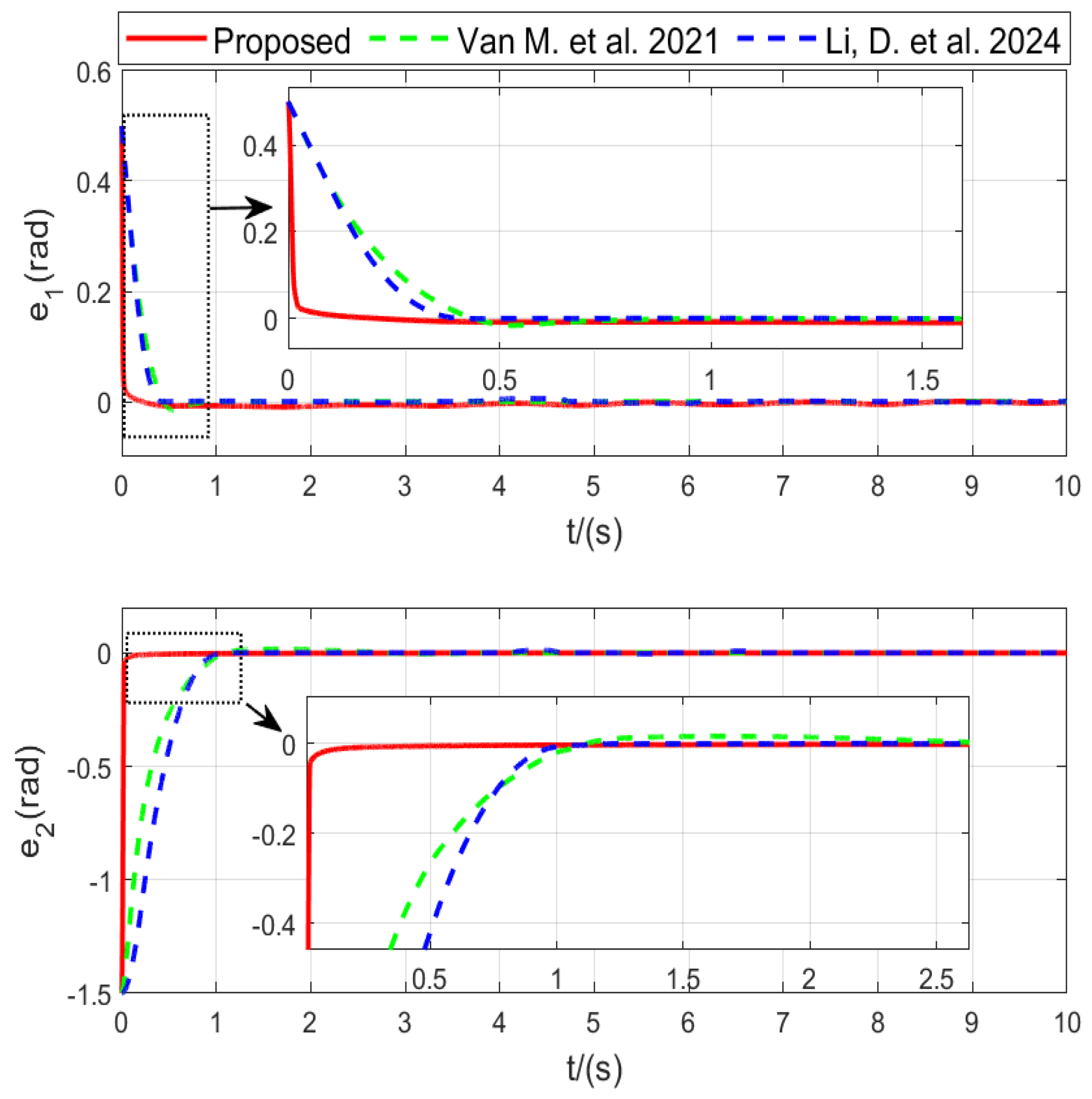
Table 2 provides a comparative performance analysis of three different methods—the proposed method and the ones from Refs. [25,27]—across multiple metrics. The proposed method significantly outperforms the others, with substantially shorter convergence times and lower steady-state errors for both e 1 and e 2 , indicating faster and more precise system responses.
Furthermore, in the proposed method, the peak values of the control inputs u 1 and u 2 are higher than those in the comparison strategy, which indicates that the control effect is strong. These results demonstrate the superiority of the proposed approach in achieving rapid convergence, high accuracy, and stable control performance, making it a promising solution for practical applications.
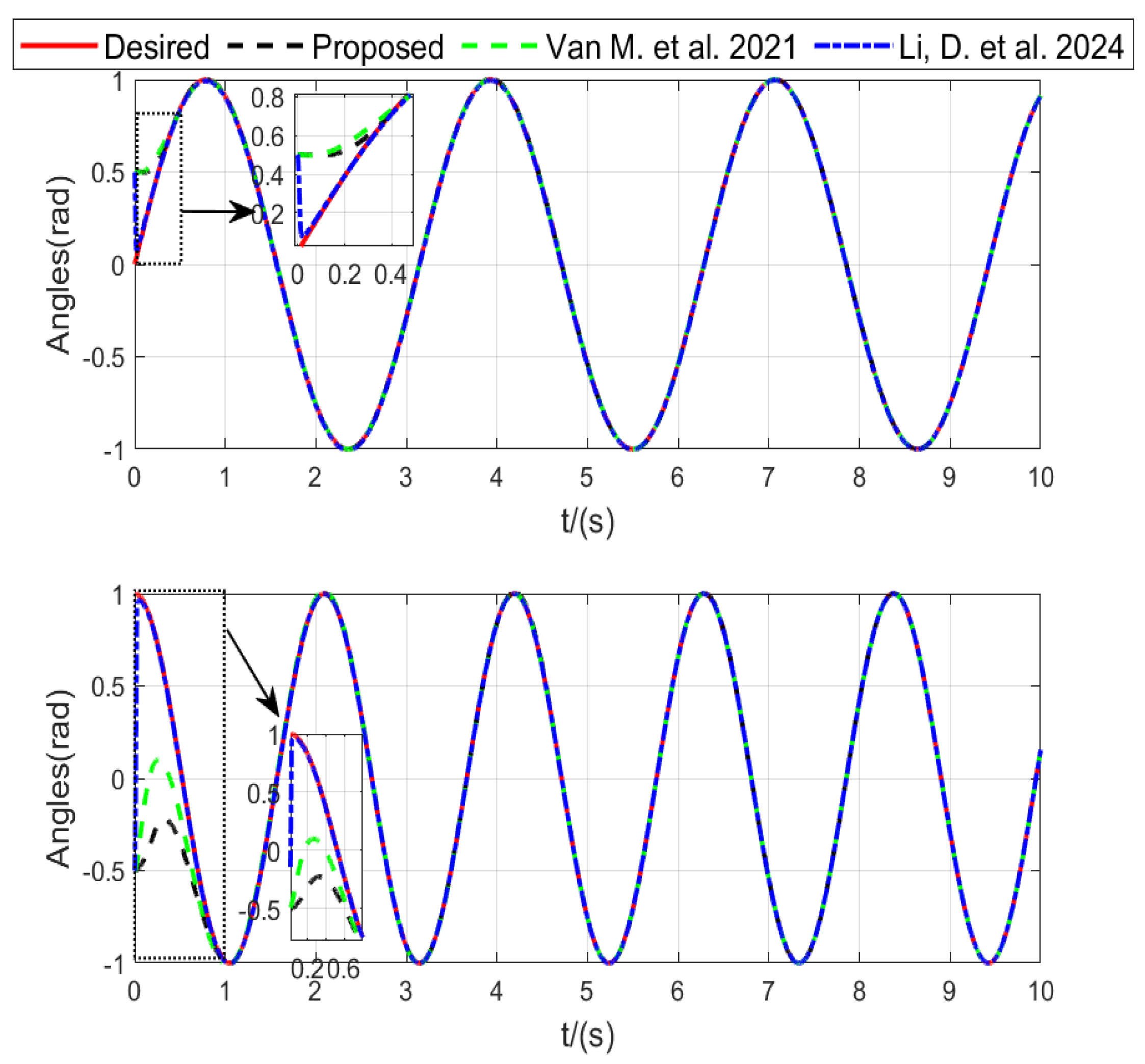
The tracking results, shown in Figure 3, provide a visual confirmation that the proposed method facilitates the swifter convergence of the manipulator to its intended trajectory.
The tracking error comparison, presented in Figure 4, also reveals that the proposed controller yields a reduced steady-state error. Additionally, the control inputs shown in Figure 5 confirm the successful mitigation of chattering by the introduced approach.
In all, the proposed controller surpasses the methodologies of [25,27] by delivering a faster convergence rate and a marked reduction in the chattering of the control input.
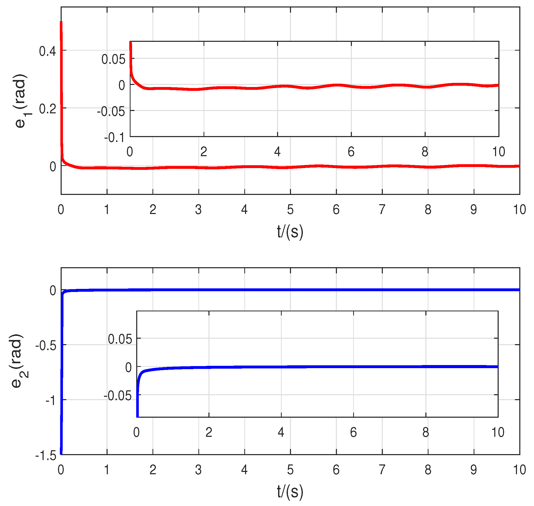
Figure 6, Figure 7 and Figure 8 show the tracking effects of the robotic manipulators after an increase in failure rate. From the figures, it can be observed that, although the failure rate is increased by 10 times, the proposed strategy still ensures the rapid and stable tracking performance of the robotic manipulators. In addition, the control inputs of the proposed strategy do not exhibit any significant chattering, avoiding the loss of mechanical components caused by high-frequency chattering. This further verifies the strong robustness of the proposed scheme.
Compared with the above, the increase in the failure rate this time is 10 times that in the aforementioned comparative experiment; this is used to verify the robustness and effectiveness of the proposed PFTC, while all other parameters remain unchanged.

5. Conclusions

This paper presents a robust adaptive control methodology, incorporating a passive FTC design, to deal with the trajectory tracking of robotic manipulators affected by model uncertainties and actuator failures. This strategy does not depend on observers and reduces the amount of calculation compared with active fault-tolerant control.
Furthermore, the adaptive law is designed to function without needing a priori knowledge of system uncertainties and disturbances. The proposed method demonstrates notable advantages, including reduced tracking errors, accelerated convergence, and a substantial improvement in the system’s robustness and transient characteristics.
Numerical simulations and comparative studies verify that the proposed strategy is robust and can effectively suppress the chattering of the control signal. It must be noted that delayed signals [28,29,30] and input saturation [31,32,33] may affect the control effects in practical engineering applications, and these are not considered in this paper. Future research will focus on physical experiments and performance verification in complex environments.

Author Contributions

This study was accomplished through the efforts of all authors. Y.W. carried out the work and performed the analysis. M.W. designed and executed the numerical simulations and wrote and reviewed the manuscript for accuracy. All authors have read and agreed to the published version of the manuscript.

Funding

This work was performed via the Dezhou Industrial Robot System Integration Engineering Research Center.

Data Availability Statement

The original contributions presented in this study are included in the article. Further inquiries can be directed to the corresponding author.

Acknowledgments

The authors express their gratitude to the anonymous reviewers for their helpful comments, which contributed significantly to enhancing the overall quality of this manuscript.

Conflicts of Interest

The authors declare no conflicts of interest.

References

  1. Yang, J.; Wang, Y.; Wang, T.; Hu, Z.; Yang, X.; Rodriguez-Andina, J.J. Time-delay sliding mode control for trajectory tracking of robot manipulators. IEEE Trans. Ind. Electron. 2024, 71, 13083–13091. [Google Scholar] [CrossRef]
  2. El Makrini, I.; Rodriguez-Guerrero, C.; Lefeber, D.; Vanderborght, B. The variable boundary layer sliding mode control: A safe and performant control for compliant joint manipulators. IEEE Robot. Autom. Lett. 2016, 2, 187–192. [Google Scholar] [CrossRef]
  3. Zhang, Y.; Kong, L.; Zhang, S.; Yu, X.; Liu, Y. Improved sliding mode control for a robotic manipulator with input deadzone and deferred constraint. IEEE Trans. Syst. Man Cybern. Syst. 2023, 53, 7814–7826. [Google Scholar] [CrossRef]
  4. Saied, H.; Chemori, A.; Bouri, M.; El Rafei, M.; Francis, C. Feedforward super-twisting sliding mode control for robotic manipulators: Application to PKMs. IEEE Trans. Robot. 2023, 39, 3167–3184. [Google Scholar] [CrossRef]
  5. Li, M.; Zhang, J.; Li, S.; Wu, F. Adaptive finite-time fault-tolerant control for the full-state-constrained robotic manipulator with novel given performance. Eng. Appl. Artif. Intell. 2023, 125, 106650. [Google Scholar] [CrossRef]
  6. Tian, G.; Tan, J.; Li, B.; Duan, G. Optimal fully actuated system approach-based trajectory tracking control for robot manipulators. IEEE Trans. Cybern. 2024, 54, 7469–7478. [Google Scholar] [CrossRef] [PubMed]
  7. Zhang, L.; Liu, H.; Tang, D.; Hou, Y.; Wang, Y. Adaptive fixed-time fault-tolerant tracking control and its application for robot manipulators. IEEE Trans. Ind. Electron. 2021, 69, 2956–2966. [Google Scholar] [CrossRef]
  8. Amin, A.A.; Iqbal, M.S.; Shahbaz, M.H. Development of intelligent fault-tolerant control systems with machine learning, deep learning, and transfer learning algorithms: A review. Expert Syst. Appl. 2024, 238, 121956. [Google Scholar] [CrossRef]
  9. Jia, F.; Cao, F.; He, X. Active fault-tolerant control against intermittent faults for state-constrained nonlinear systems. IEEE Trans. Syst. Man Cybern. Syst. 2024, 54, 2389–2401. [Google Scholar] [CrossRef]
  10. Jia, F.; He, X. Active fault-tolerant control with adaptive estimation error compensation for nonlinear systems: Achieving asymptotic tracking. IEEE Trans. Ind. Inform. 2024, 20, 6612–6621. [Google Scholar] [CrossRef]
  11. Milecki, A.; Nowak, P. Review of fault-tolerant control systems used in robotic manipulators. Appl. Sci. 2023, 13, 2675. [Google Scholar] [CrossRef]
  12. Jadidi, S.; Badihi, H.; Zhang, Y. Enhancing Hierarchical Fault-Tolerant Cooperative Control in Wind Farms: The Application of Model Predictive Control and Control Reallocation. In Proceedings of the 2023 12th International Conference on Renewable Energy Research and Applications (ICRERA), Oshawa, ON, Canada, 29 August–1 September 2023; pp. 429–434. [Google Scholar]
  13. Kang, E.; Qiao, H.; Chen, Z.; Gao, J. Tracking of uncertain robotic manipulators using event-triggered model predictive control with learning terminal cost. IEEE Trans. Autom. Sci. Eng. 2022, 19, 2801–2815. [Google Scholar] [CrossRef]
  14. El-Hussieny, H.; Hameed, I.A.; Megahed, T.F.; Fares, A. Advancing Robotic Control: Data-Driven Model Predictive Control for a 7-DOF Robotic Manipulator. IEEE Access 2024, 12, 115926–115934. [Google Scholar] [CrossRef]
  15. Son, J.; Kang, H.; Kang, S.H. A review on robust control of robot manipulators for future manufacturing. Int. J. Precis. Eng. Manuf. 2023, 24, 1083–1102. [Google Scholar] [CrossRef]
  16. Silaa, M.Y.; Barambones, O.; Bencherif, A.; Rougab, I. An Adaptive Control Strategy with Switching Gain and Forgetting Factor for a Robotic Arm Manipulator. Machines 2025, 13, 424. [Google Scholar] [CrossRef]
  17. Xu, S.S.D.; Chen, C.C.; Wu, Z.L. Study of nonsingular fast terminal sliding-mode fault-tolerant control. IEEE Trans. Ind. Electron. 2015, 62, 3906–3913. [Google Scholar] [CrossRef]
  18. Li, W.; Zhang, Z.; Wang, P.; Wan, H. A Faster Fixed-Time Fault Tolerant Sliding Mode Control for Robot Manipulators with Mismatched Disturbances. IEEE Access 2025, 13, 56576–56586. [Google Scholar] [CrossRef]
  19. Nguyen, V.C.; Vo, A.T.; Kang, H.J. A finite-time fault-tolerant control using non-singular fast terminal sliding mode control and third-order sliding mode observer for robotic manipulators. IEEE Access 2021, 9, 31225–31235. [Google Scholar] [CrossRef]
  20. Nguyen, V.C.; Tran, X.T.; Kang, H.J. A novel high-speed third-order sliding mode observer for fault-tolerant control problem of robot manipulators. Actuators 2022, 11, 259. [Google Scholar] [CrossRef]
  21. Montanaro, U.; Martini, S.; Hao, Z.; Gao, Y.; Sorniotti, A. Multi-input enhanced model reference adaptive control strategies and their application to space robotic manipulators. Int. J. Robust Nonlinear Control 2023, 33, 5246–5272. [Google Scholar] [CrossRef]
  22. Obuz, S.; Tatlicioglu, E.; Zergeroglu, E. Adaptive Cartesian space control of robotic manipulators: A concurrent learning based approach. J. Frankl. Inst. 2024, 361, 106701. [Google Scholar] [CrossRef]
  23. Jiang, J.; Yu, X. Fault-tolerant control systems: A comparative study between active and passive approaches. Annu. Rev. Control 2012, 36, 60–72. [Google Scholar] [CrossRef]
  24. Liu, Z.; Zhao, Y.; Zhang, O.; Chen, W.; Wang, J.; Gao, Y.; Liu, J. A novel faster fixed-time adaptive control for robotic systems with input saturation. IEEE Trans. Ind. Electron. 2023, 71, 5215–5223. [Google Scholar] [CrossRef]
  25. Van, M.; Ceglarek, D. Robust fault tolerant control of robot manipulators with global fixed-time convergence. J. Frankl. Inst. 2021, 358, 699–722. [Google Scholar] [CrossRef]
  26. Asl, R.M.; Hagh, Y.S.; Palm, R.; Handroos, H. Integral non-singular terminal sliding mode controller for nth-order nonlinear systems. IEEE Access 2019, 7, 102792–102802. [Google Scholar]
  27. Li, D.; Chen, M.; Peng, K.; Wu, L. Fixed-time fault-tolerant control of manipulator systems based on sliding mode observer. Int. J. Robust Nonlinear Control 2024, 34, 440–455. [Google Scholar] [CrossRef]
  28. Peng, Z.; Chen, H.; Zheng, J.; Zhang, J.; Xue, M.A.; Long, X.; Zhou, W. Tracking control of underactuated surface vessel based on decoupled cascaded system design with input saturation and time delay. Int. J. Control 2025, 1–9. [Google Scholar] [CrossRef]
  29. Xu, R.; Chen, H.; Tang, Y.; Long, X. Model-free predictive iterative learning safety-critical consensus control for multi-agent systems with randomly varying trial lengths. Syst. Control Lett. 2025, 196, 105987. [Google Scholar] [CrossRef]
  30. Long, X.; Chen, H.; Zheng, J.; Zhang, J.; Xue, M.A.; Tang, Y.; Xu, R.; Zhao, Y. Nonfragile memory-based sampled-data control for Unmanned Surface Vehicles with time-varying coupling delay. Ocean Eng. 2024, 313, 119480. [Google Scholar] [CrossRef]
  31. Liu, Z.; Zhang, O.; Gao, Y.; Zhao, Y.; Sun, Y.; Liu, J. Adaptive neural network-based fixed-time control for trajectory tracking of robotic systems. IEEE Trans. Circuits Syst. II Express Briefs 2022, 70, 241–245. [Google Scholar] [CrossRef]
  32. Liu, Z.; Liu, J.; Zhang, O.; Zhao, Y.; Chen, W.; Gao, Y. Adaptive disturbance observer-based fixed-time tracking control for uncertain robotic systems. IEEE Trans. Ind. Electron. 2024, 71, 14823–14831. [Google Scholar] [CrossRef]
  33. Liu, J.; Sun, Y.; Liu, Z.; Gao, Y.; Wu, L.; Leon, J.I.; Franquelo, L.G. Predefined-Time Reliable Control for Robotic Systems With Prescribed Performance. IEEE Trans. Ind. Electron. 2025. [Google Scholar] [CrossRef]
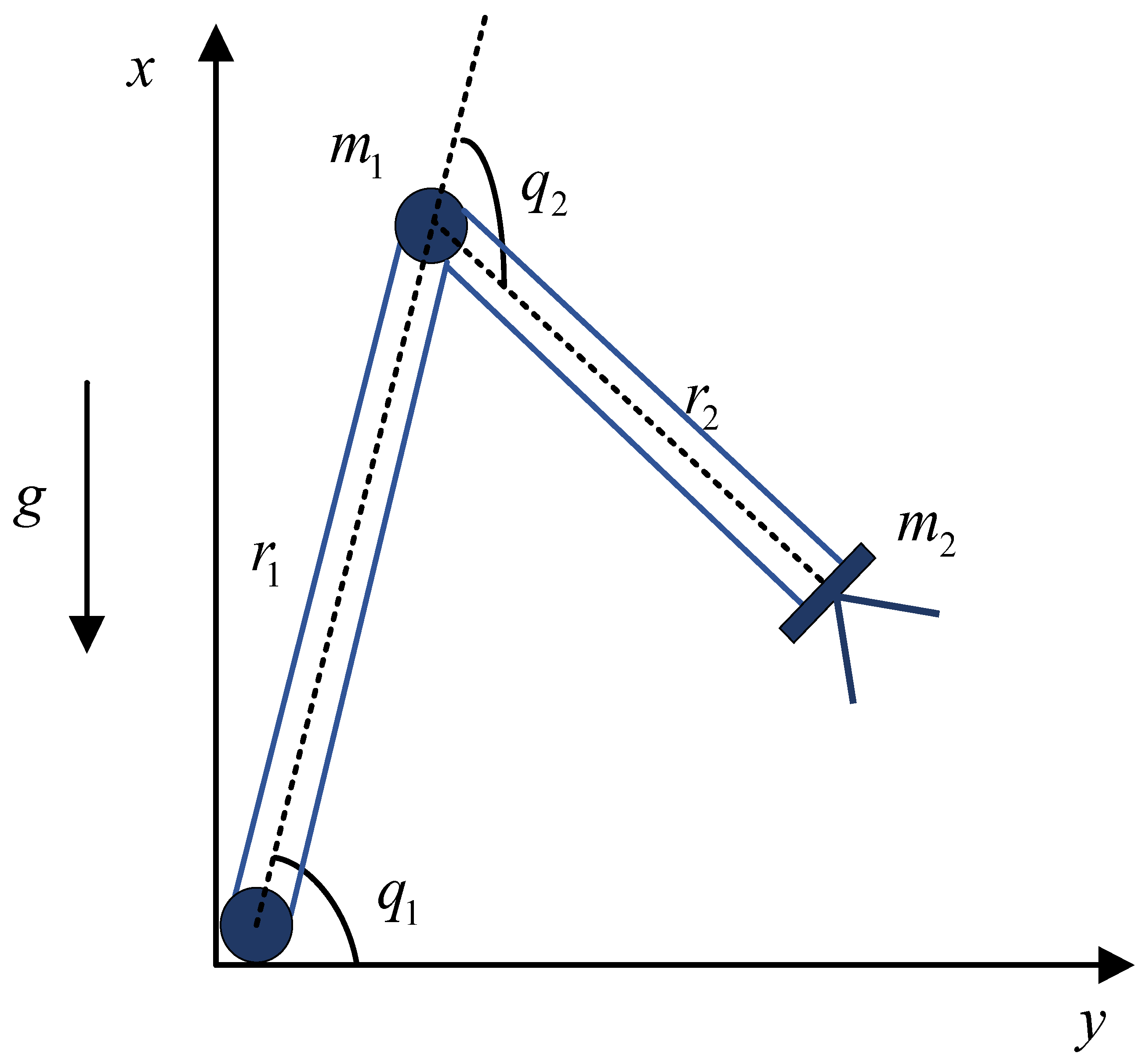
Figure 1. Schematic representation of the robot manipulator system.
Symmetry 17 01547 g001
Figure 2. Flow chart of proposed controller.
Symmetry 17 01547 g002
Figure 3. Tracking performance of manipulators with Refs. [25,27].
Symmetry 17 01547 g003
Figure 4. Tracking error comparison with Refs. [25,27].
Symmetry 17 01547 g004
Figure 5. Control input comparison with Refs. [25,27].
Symmetry 17 01547 g005
Figure 6. Tracking performance of manipulators.
Symmetry 17 01547 g006
Figure 7. Tracking error comparison.
Symmetry 17 01547 g007
Figure 8. Control input.
Symmetry 17 01547 g008
Table 1. Dynamic parameters.
ParameterValueParameterValue
r 1 1 m r 2 1 m
m 1 10 kg m 2 1 kg
m 01 9.8 kg m 02 0.98 kg
Δ m 1 0.2 kg Δ m 2 0.02 kg
g9.8 m / s 2
Table 2. Performance comparison.
MethodProposedRef. [25]Ref. [27]
C o n v e r g e n c e T i m e o f e 1 ( s ) 0.1430.3780.512
C o n v e r g e n c e T i m e o f e 2 ( s ) 0.8141.0391.181
S t e a d y S t a t e E r r o r o f e 1 ( s ) 0.00360.00820.0080
S t e a d y S t a t e E r r o r o f e 2 ( s ) 0.03750.04480.0579
P e a k V a l u e o f u 1 ( s ) 982.02487.35221.4
P e a k V a l u e o f u 2 ( s ) 79.464253.1429.781
Disclaimer/Publisher’s Note: The statements, opinions and data contained in all publications are solely those of the individual author(s) and contributor(s) and not of MDPI and/or the editor(s). MDPI and/or the editor(s) disclaim responsibility for any injury to people or property resulting from any ideas, methods, instructions or products referred to in the content.