Monitoring and Diagnostics of Mining Electromechanical Equipment Based on Machine Learning

Abstract

Induction motors are a common component of electromechanical equipment in mining operations, yet they are susceptible to failures resulting from frequent start–stops, overloading, wear and tear, and component failure. It is evident that such failures can result in severe ramifications, encompassing industrial accidents and economic losses. The present paper proposes a detailed study of engine fault diagnosis technology. It has been demonstrated that prevailing intelligent engine diagnosis algorithms exhibit a limited diagnostic efficacy under variable operating conditions, and the reliability of diagnostic outcomes based on individual signals is questionable. The present paper puts forward the proposition of an investigation into a fault diagnosis algorithm for induction motors. This investigation utilized a range of analytical methods, including signal analysis, deep learning, transfer learning, and information fusion. Currently, the methods employed for fault diagnosis based on traditional machine learning are reliant on the selection of statistical features by those with expertise in the field, resulting in outcomes that are significantly influenced by human factors. This paper is the first to integrate a multi-branch ResNet strategy combining three-phase and single-phase currents. A range of three-phase current input strategies were developed, and a deep learning-based motor fault diagnosis model with adaptive feature extraction was established. This enables the deep residual network to extract fault depth features from the motor current signal more effectively. The experimental findings demonstrate that deep learning possesses the capacity to automatically extract depth features, thereby exceeding the capabilities of conventional machine learning algorithms with regard to the accuracy of motor fault diagnosis.

1. Introduction

As a significant source of kinetic energy in industrial and agricultural production, induction motors offer several advantages, including their simple construction, ease of dismantling, low manufacturing cost, high reliability, and durability. Their utilization is extensive, encompassing mining equipment and metallurgy, machine tools, power plants, fans, and a range of other industrial sectors. The reliable and stable operation of motors is not only related to the stable and long-term operation of individual mechanical equipment but also affects the stability of the entire production system. In the event of an induction motor failure, the operation of the equipment is interrupted, the operating efficiency is reduced, and the energy consumption increases. In severe cases, the entire system is destroyed, resulting in significant economic losses and casualties. Furthermore, the elimination of sudden failures is challenging, which results in increased damage. The prevailing paradigm concerning the safety management of induction motors is predicated on the notion of regular maintenance. The efficacy of the motor is determined by conducting a thorough examination and repair of its various components. This approach, however, is often characterized by a lack of systematic maintenance and a consequent wastage of resources. The advent of the Internet of Things has engendered a paradigm shift in the realm of industrial automation, paving the way for the real-time monitoring of the operational status of induction motors. This advancement has been made possible by the integration of advanced sensor technology, which has emerged as a pivotal component in the digital transformation of industrial infrastructure. Consequently, the development of methodologies for the early online diagnosis of motor faults, based on the analysis of collected signals, has become a major area of research. Conventional motor fault diagnosis frequently relies on threshold evaluation methods. However, induction motors typically operate in complex conditions, and the early characteristics of the fault are often obscured by noise, leading to delayed fault detection and subsequent motor repair. Presently, industrial machinery as a whole is undergoing a process of automation and intelligence, with the development of artificial intelligence algorithms being a significant factor in this transformation. Concurrently, technological advancements in fault diagnosis are facilitating the updating of these systems. Intelligent diagnosis algorithms, which do not require expert experience, have been shown to have advantages such as good diagnostic effect and high stability, and they find application in the field of motor fault diagnosis [1,2,3]. In recent years, research has focused on cross-working transfer learning to solve the problem of data distribution differences. Zhu et al. (2020) [4] proposed an adversarial domain adaptation method to improve the robustness of bearing variable speed diagnosis. In [4] Yan et al. (2021) verified the superiority of transfer learning in shearer rocker composite fault identification.

The field of engine fault diagnosis encompasses a range of techniques, which can be categorized into four distinct groups: signal-based, mechanical theory-based, model-based, and simulation-based techniques [4,5]. In view of the above shortcomings, this study proposes a motor diagnosis framework that integrates real working condition data and open-set transfer learning to solve the problems of cross-working condition generalization and unknown fault identification in complex mining environments. In the nascent stages of development, algorithms for fault diagnosis based on mechanical theory were particularly prevalent [6,7,8,9]. The investigation primarily entailed a theoretical examination of the manifestations of various engine faults. However, the creation of a mathematical model capable of accurately describing the fault mechanism was unsuccessful, and the model was unable to reflect the real working condition of the engine, which was evidently disadvantageous. The advent of signal detection technology, signal processing, and artificial intelligence algorithms has precipitated the evolution of signal-based fault diagnosis algorithms and those based on traditional machine learning models [10,11]. In the domain of fault diagnosis, these systems boast significant advantages, including high diagnostic efficiency, rapid processing speeds, and accurate results. The primary challenge at present is the necessity for manual feature selection, which necessitates a substantial volume of data for network training. A simulation-based fault diagnosis algorithm principally employs popular numerical simulation software to create an efficient physical model analogous to a real motor, producing responses such as current, vibration, and even acoustic signals that intuitively reflect the physical changes of the motor during operation [12,13,14]. The advent of the era of big data and artificial intelligence has precipitated the gradual replacement of traditional intelligent algorithms with intelligent fault diagnosis technology based on deep learning algorithms. Deep learning, which has become the primary research direction in the current era, has been extensively studied and evaluated in the domain of motor fault diagnosis.

It is important to note that each diagnostic algorithm has its own advantages and limitations. Existing intelligent diagnostic algorithms have been shown to lack accuracy in the diagnosis of cross-domain faults, with the majority requiring a substantial amount of training data. In the context of real machinery, given that the equipment is generally in working condition during operation, faults tend to manifest within a very brief timeframe. This results in an absence of adequate fault data and imbalanced samples [15,16,17]. This study proposes a multi-branch current input strategy, realizes cross-condition migration diagnosis, and verifies the robustness of ResNet in industrial scenarios. The experimental results show that diagnostic accuracy was improved by 3.2–4.6%, and transfer learning reduced the training data requirements by 40%.

2. Materials and Methods

2.1. Types of Engine Malfunctions

If the motor is frequently started and stopped, the rotor bars may break due to uneven force. Load variations and voltage fluctuations can also affect the service life, leading to rotor breakage (Figure 1).

In the event of a fault occurring, the characteristic frequency expression of the rotor is as follows:

$$f_{bb}=\left(1\pm 2ks\right)f_1,$$

(1)

where s is the slip velocity; f₁ is the power frequency; and k is a positive integer.

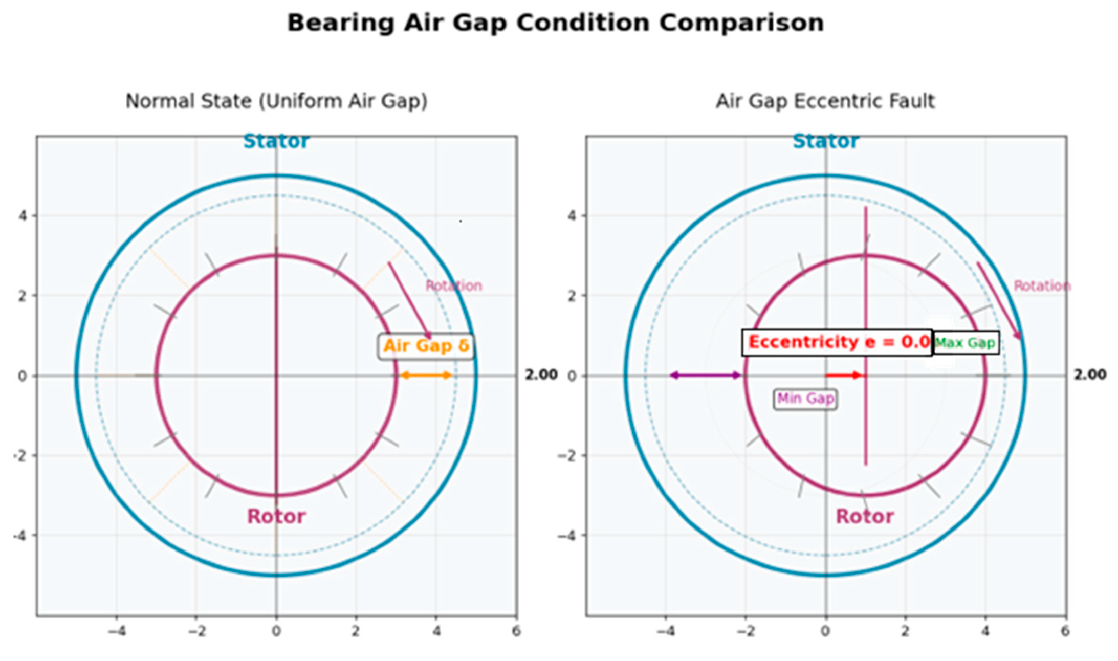
The air gap between the rotor and stator of the motor is not uniformly distributed (Figure 2).

The expression of the frequency of the fault characteristic is as follows:

$$f_{ag}=\left[{\displaystyle \frac{\left(n_{rt}{Z}_2\pm n_d\right)\left(1-s\right)}{p}}\pm n_{ws}\right]f_1,$$

(2)

where Z₂ is the number of rotor slots, n_rt, n_d, and n_ws are integers; and the value of nd depends on the type of fault. At static eccentricity, n_d = 0. At dynamic eccentricity, n_d = 1, 2, 3, …; p is the number of pole pairs of the magnetic field of the motor.

The simplified expression of the frequency of the fault characteristic is as follows:

$$f_{ag}=f_1\pm m{f}_r,$$

(3)

where m is a positive integer, y is the rotor speed, and the expression has the following form:

$$f_r={\displaystyle \frac{\left(1-s\right)f_1}{p}}$$

(4)

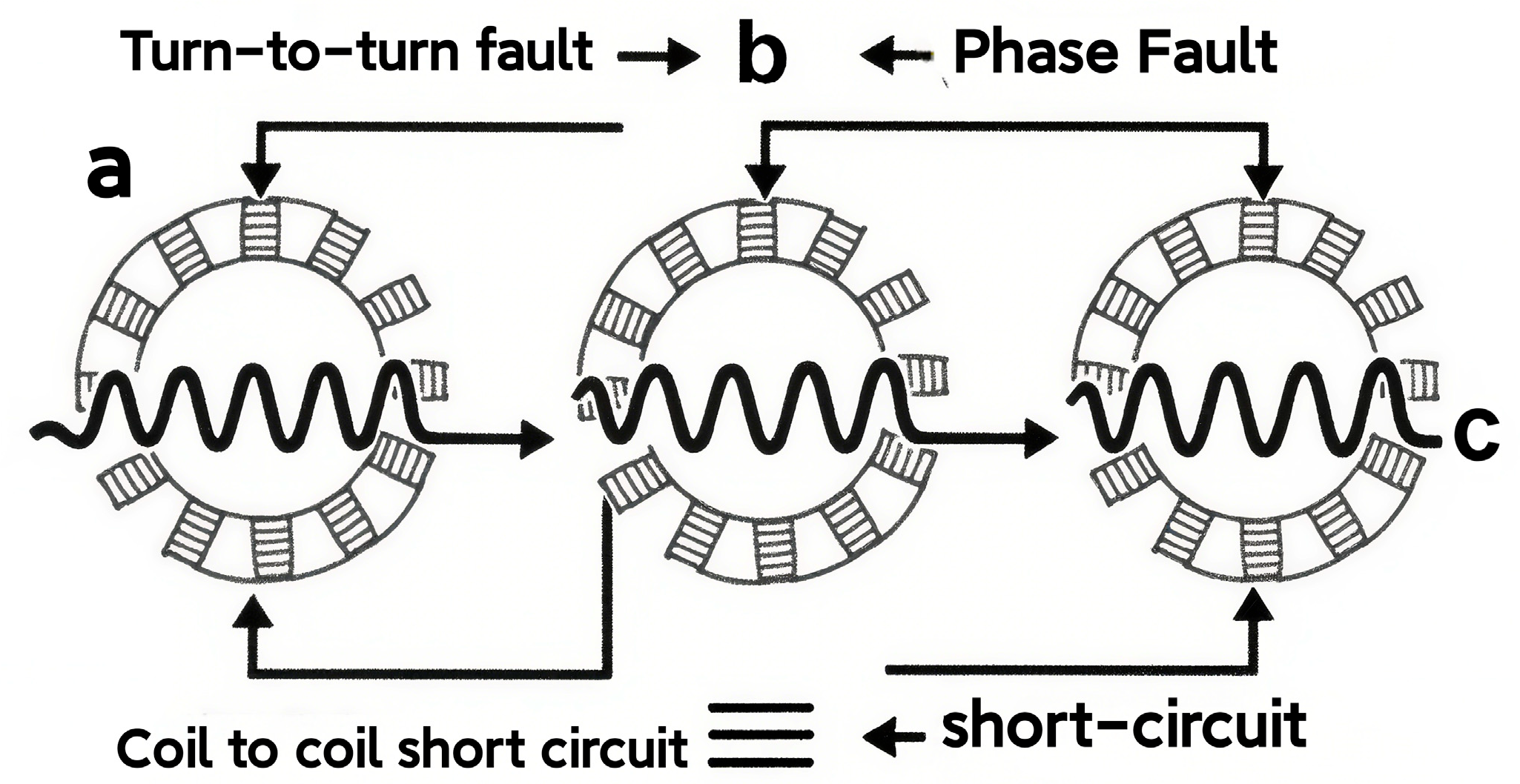
One of the types of stator failure that has been identified is winding-to-winding stator failure, a fault that has been observed to be prevalent in induction motors. The phenomenon under investigation consists of the insulation between two or more neighboring turns of the stator winding being damaged, resulting in current leakage (Figure 3).

In the event of a fault, the stator current waveform is distorted, and harmonic components appear. The specific expression of the harmonic component characteristic of a fault is as follows:

$$f_{st}=\left[{\displaystyle \frac{n}{p}}\left(1-s\right)\pm z\right]f_1=n{f}_r\pm z{f}_1,$$

(5)

where z = 1, 2, 3, …, (2p − 1); n = 1, 3, 5, …

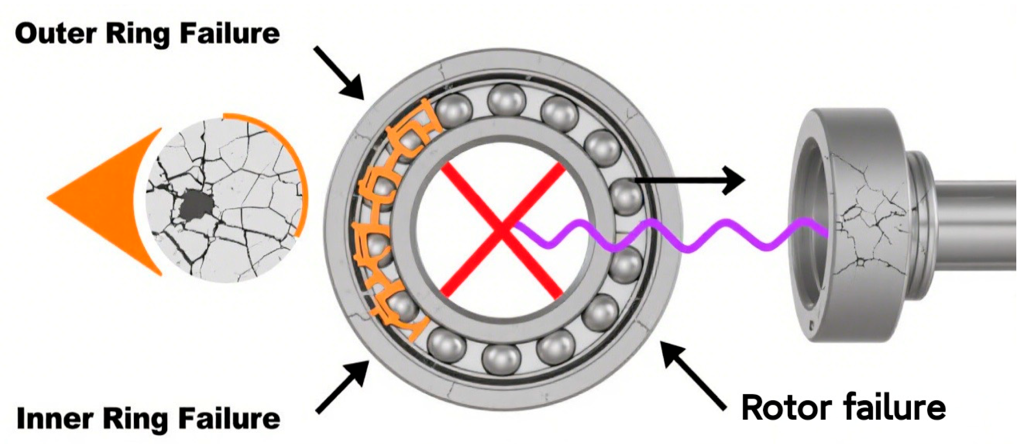
Bearings are frequently subjected to suboptimal conditions, including extended operation, overloading, corrosion, and wear, which can readily result in the failure of various components within the bearing. At this time, the motor produces abnormal oscillations, causing changes in the magnetic field, thereby generating harmonics in the stator current (see Figure 4).

Faults in different parts of the bearing generate vibration information of certain frequencies, and their vibration characteristics are different from each other [18,19,20].

The failure of the inner ring of the f_bi is expressed as

$$f_{bi}={\displaystyle \frac{Nn}{120}}\left(1+{\displaystyle \frac{d}{D}}\cos \alpha \right)$$

(6)

f_bo destruction of the exterior ring is expressed as

$$f_{bo}={\displaystyle \frac{Nn}{120}}\left(1-{\displaystyle \frac{d}{D}}\cos \alpha \right)$$

(7)

Failure of the rolling elements f_br is expressed as

$$f_{br}={\displaystyle \frac{n}{120}}\left(1-{\displaystyle \frac{d}{D}}\cos \alpha \right)$$

(8)

Cage failure f_bc is expressed as

$$f_{bc}={\displaystyle \frac{Dn}{120d}}\left[1-{\left({\displaystyle \frac{d}{D}}\right)}^2{cos}^2\alpha \right]$$

(9)

2.2. Traditional Method of Current Signal Analysis

An improved discrete Fourier transform (DFT) algorithm reduces the signal analysis time and provides frequency information of the current signal [21,22,23].

For a sequence X[n] of length N, its DFT is defined as

$$X\left[k\right]={\sum }_{n=0}^{N-1}x\left[n\right]\times e^{\raisebox{1ex}{$-j2\pi kn$}\!\left/ \!\raisebox{-1ex}{$N$}\right.,}$$

(10)

where X[k] is the k-th DFT coefficient of the sequence x[n], x[n] is the original sequence, N is the length of the sequence, k is the frequency index, k = 0, 1, 2, …, N − 1, and j is the imaginary unit satisfying j = −1.

The fast Fourier transform (FFT) is an efficient algorithm for computing the FFT. In the context of a sequence of length N, the fast Fourier transform (FFT) leverages the symmetry and periodicity inherent to the transform to reduce the complexity from O(N²) to O(N log N).

The elimination of the influence of the supply frequency is achieved by converting the three-phase stator current signal into a two-phase orthogonal DC signal (d–q coordinate system). This process highlights the fault characteristics in the signal.

• Clarke Transform: The three-phase current signal is converted into a two-phase orthogonal signal (α–β coordinate system).
• Park’s Transform: The following investigation concerns the conversion of a two-phase orthogonal signal to a d–q coordinate system in a synchronous rotating coordinate system.
  The electrical angle of the motor rotor, denoted by θ, can be determined from the time-varying rotor position.
• An analysis of fault signs is required. In the d–q coordinate system, the analysis of current components on the d- and q-axes enables the determination of various fault signs.

2.3. Convolutional Neural Networks

Deep learning is a subset of machine learning that falls under the umbrella of neural networks. The name itself alludes to the fact that deep learning networks are characterized by their ability to learn at a more profound level. In comparison with conventional machine learning algorithms, deep learning has the capacity to discern characteristics that are not explicable within the dataset by emulating the cognitive processes of the human brain. Additionally, it possesses the capability to extract latent features. To date, deep learning has encompassed a variety of conventional models. The deployment of distinct models in disparate domains is predicated on the unique characteristics of their respective networks. Convolutional neural networks (CNNs) represent a prominent example of deep learning networks. The feed-forward neural network under consideration has multiple convolutional and merging layers, making it well-suited to image processing. In this paper, a CNN was utilized for the extraction of deep features from source signals, with the objective of investigating engine fault diagnosis (Figure 5).

Convolutional neural networks (CNNs) have been shown to share parameters and local perceptual strategies with the aim of reducing computation time. The primary application of these models is in the domain of engine fault diagnosis. In this context, they are employed either for the extraction and recognition of features or as a direct classifier. This model consists of an input layer, a convolution layer, an association layer, a fully connected layer, and an output layer [24,25,26].

In addition to the initial LeNet model, CNNs encompass AlexNet, VGG-Nets, ResNet, and other variants. Alex-Net is composed of two structures, one upper and one lower, which can be trained in parallel on two GPUs, thereby reducing the training time of the network [27,28,29]. VGG-Nets exhibit strong generalization ability, and the pre-trained parameters can be directly transferred to other tasks [30]. The model is distinguished by a more intricate network, with the dimensionality of the input data progressively diminishing across successive layers. 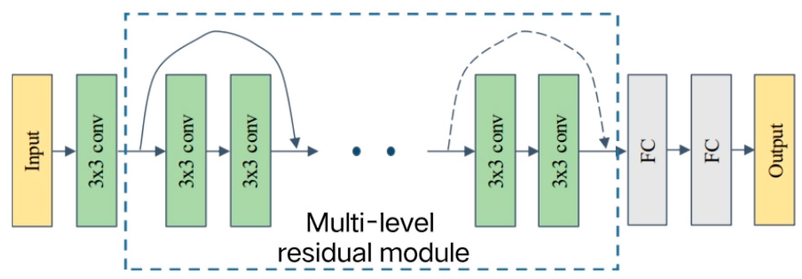ResNet employs residual modules, a strategy that not only streamlines the objectives and intricacy of training as the network depth increases but also utilizes a straightforward stochastic gradient descent method for network training [31,32,33]. In comparison with VGG networks, this approach entails a reduction in network parameters and a diminution of the risk of overestimation. Consequently, all deep learning networks discussed in this paper employ ResNet. The following section provides a comprehensive delineation of the ResNet architecture. A ResNet-based deep network, i.e., a deep residual network, constructs residual blocks to allow the transfer of gradients between layers in the backpropagation process. This reduces the complexity of model training and optimizes network performance. ResNet-based deep networks, which are frequently employed, demonstrate variability in their depth. The structure incorporates convolutional layers, multi-layer residual blocks with variable numbers of residual blocks, and fully connected layers. The configuration of the ResNet18 network, comprising 18 weight layers, is illustrated in Figure 6.

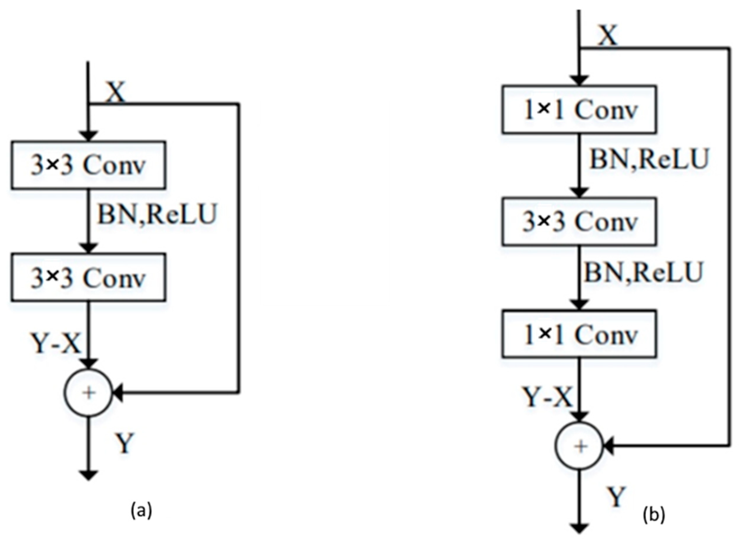
There are 8 residual modules in the whole network; the structure of the residual modules is shown in Figure 7.

As shown in the figure, the design is divided into a residual module and a down-sampled residual module, depending on whether it contains down-sampling. When the input is X and the output of the model is Y, the residual module should learn the residual mapping, Y–X, which solves the problem of gradient disappearance in traditional CNNs as the network layer deepens and protects the integrity of data information. In the residual module, BN (batch normalization) is used to normalize the output data of each node. It includes two steps:

(1)

Normalization: Firstly, the mean and variance are calculated, the vector x is normalized, where the vector contains m data, i.e., x = {x1, x2, …, xm}, and, finally, a distribution of data $\widehat{\mathrm{x}}$ with zero mean and unit variance is obtained.

(2)

Scaling and translation: We scale and translate $\widehat{\mathrm{x}}$ to obtain a new data distribution yi with the mean β and the variance γ.

Despite the recent emergence of new architectures, such as the vision transformer, ResNet is particularly suitable for processing high-noise current signals due to the stability of its residual structure in gradient propagation and feature extraction. In addition, SVM serves as a benchmark model, facilitating comparison with the classical literature (e.g., Tang et al., 2020 [34]) and highlighting the advantages of automatic feature extraction in deep learning.

2.4. Engine Fault Diagnosis System Based on Deep Residual Network

Compared with traditional multi-signal-processing methods [35], the innovative design of this framework lies in the following:

(1)

Dual-path feature extraction: A single-phase branch (capturing local anomalies) and a three-phase branch (modeling system-level faults) work in parallel;

(2)

Dynamic fusion gating: Feature combination weights are automatically optimized through gated recurrent units (GRUs);

(3)

Computational efficiency: A 17% reduction in the parameter count compared with traditional serial networks is obtained.

The integration of data collected by multiple sensors has been demonstrated to enhance the identification of fault signs, thus providing a significant advantage over single-signal classification methods. Information fusion can be categorized into three distinct levels: data-level fusion, feature-level fusion, and decision-level fusion. Data-level fusion employs a range of sophisticated algorithms, including weighted average, Kalman filtering, and others, to facilitate low-level information fusion for disparate raw data. Feature-level fusion is a process that performs signal processing and feature extraction from different raw data. These features are then combined into a single vector for the purpose of fault diagnosis. Decision-level fusion employs distinct source signals to predict classification results independently, subsequently leveraging D-S evidence theory and alternative methods to perform diagnosis based on the predicted results. The latter two fusion methods involve high-level intelligent signal fusion and have gradually replaced the diagnostic methods using only data fusion in the research of intelligent engine diagnosis. Existing intelligent engine fault diagnosis algorithms based on information fusion principally utilize shallow networks for feature extraction and are, thus, incapable of extracting deep signal features. In this chapter, a deep network based on ResNet is utilized for the extraction of deep features of current signals, and Softmax is employed for the purpose of outputting the diagnostic results.

For the original three-phase stator currents collected in different states of the real motor, the waveforms in the time domain are different. In the normal state, the current waveform is subject to the influence of disturbances alone. The three-phase current amplitudes are slightly different, and the phase difference is close to 120 degrees. In the case of a rod break rotor fault, the current amplitude is oscillatory due to the influence of rod break harmonics compared with the normal state, and the oscillation rate is related to the degree of fault. In the context of an air gap eccentricity fault, the current peak undergoes distortion due to the influence of eccentricity harmonics in comparison with the normal state. However, it is noteworthy that these harmonics typically manifest in the high-frequency range. The overall waveform, nevertheless, remains comparable to the normal state.

In the case of a stator inter-turn short-circuit, the phase current amplitude assumes a significant proportion. Analysis demonstrates that, in the presence of diverse faults, the current amplitude, phase, waveform, and other parameters are subject to alterations. It is evident that there has been a shift and discrepancy in the fault characteristics when compared with previous observations. It is evident that these differences have given rise to the development of a variety of three-phase current injection strategies and the corresponding deep networks that are associated with them.

The first input strategy utilizes a multi-channel deep learning network. The three-phase current is regarded as a single unit and is directed to a 3-channel deep learning network for the purpose of feature extraction. The features are then superimposed following convolution. The present framework is principally concerned with the relationship between the three-phase currents (see Figure 8).

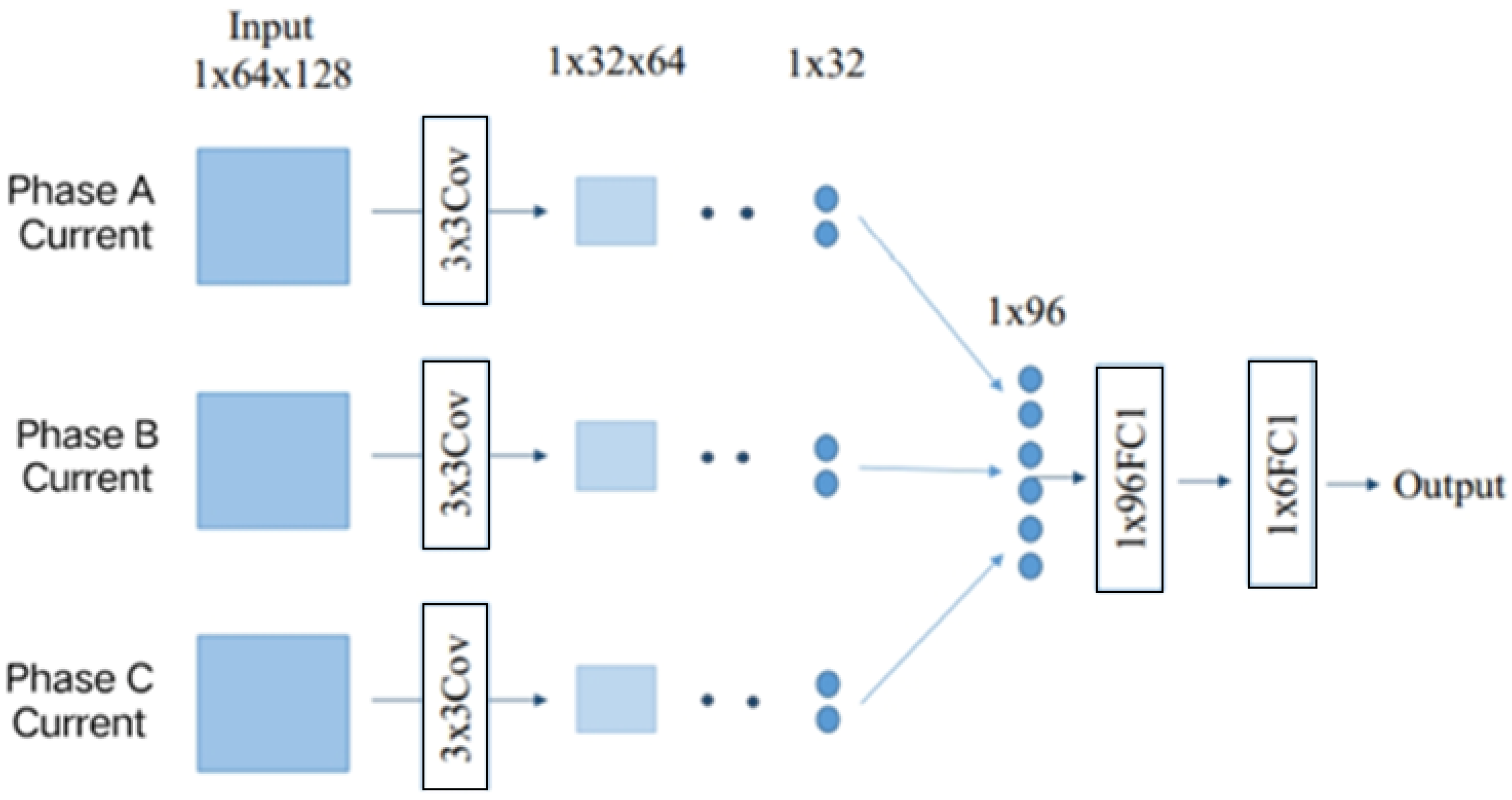
The second input strategy involves the implementation of a three-link deep learning network. The A-phase, B-phase, and C-phase currents are utilized as inputs for networks with distinct parameters, respectively. The deep characteristics of the three-phase currents are extracted, and these characteristics are subsequently fused in a fully connected layer (Figure 8). The focus of this structure is on the response of single-phase current in the event of a motor fault.

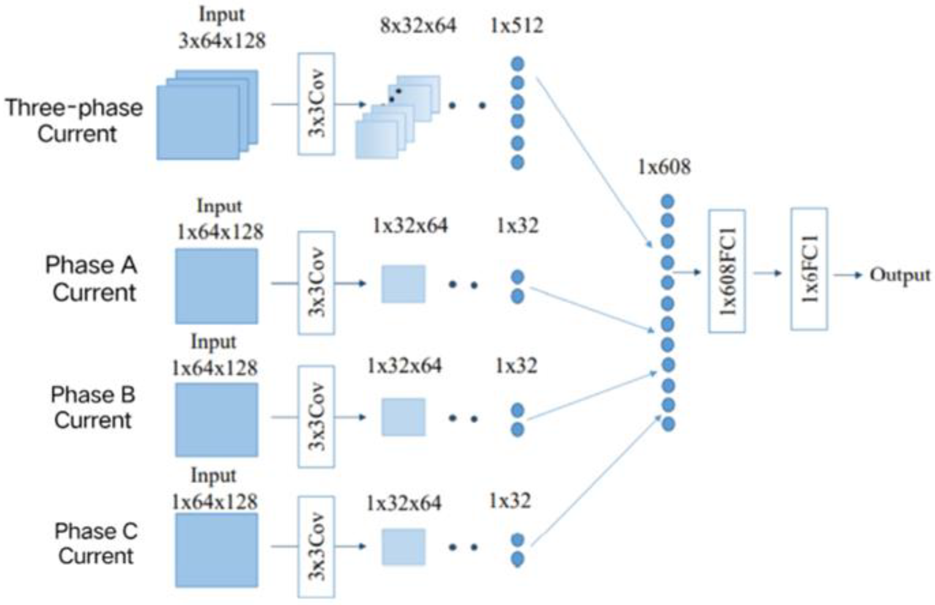
The third input strategy involves the implementation of a four-branch deep learning network. This network is designed to facilitate the extraction of features through the transmission of a three-phase current and a single-phase current to three-channel and single-channel networks, respectively. Subsequently, these features are processed through a fully connected layer to achieve feature fusion (Figure 9). This theoretical framework does not merely emphasize the relationship between the three-phase currents but also highlights the dynamic nature of the phase current itself.

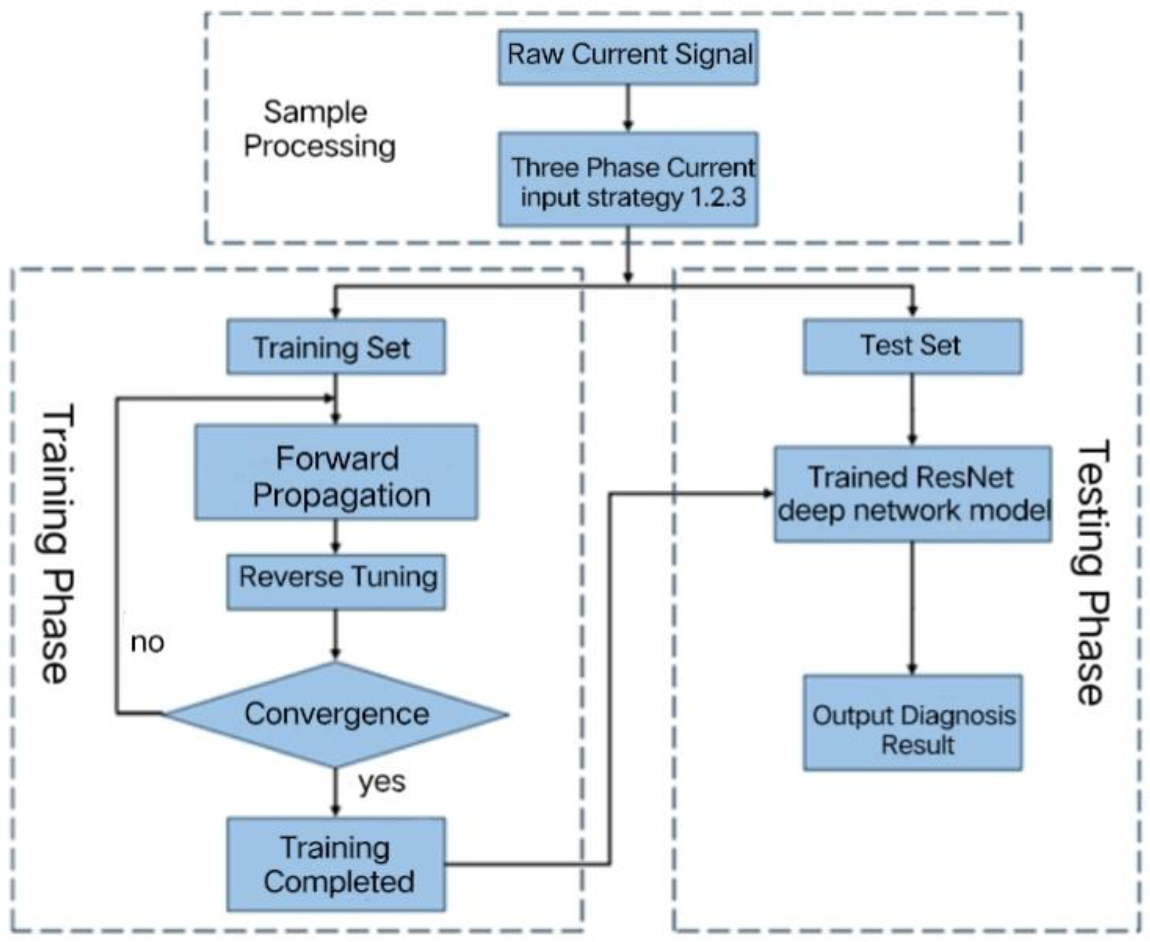
The ResNet-based deep learning algorithm for engine fault diagnosis includes three steps: sample processing, model training, and model testing (Figure 10).

As shown in Figure 10, the specific steps of the algorithm are described as follows:

(1)

Sample processing: The collected original three-phase current signal in the time domain is size-corrected and converted into a sample of size 3 × 64 × 128. For different current input strategies, the samples are divided into training and test sets. In order to simulate real working conditions more accurately, fault data should vary in quantity. Supplementing unbalanced experiments (with a fault/normal sample ratio of 5:1) will yield better results.

(2)

Training phase: The weights and parameters of the deep ResNet are initialized, the training set is used to perform forward propagation and backward optimization of the deep network, and the network parameters are backward-updated by minimizing the loss function. When the loss function or diagnostic accuracy converges in the final training phase, it means that the training of the network is complete.

(3)

Test phase: The test set is sent to the trained deep ResNet, the sample state is predicted, and the fault diagnosis accuracy is output.

3. Results and Discussion

In order to analyze the diagnostic effect of the above diagnostic model, the experiment used a YE3-132S-4 three-phase asynchronous motor (Fancy PUMP (Zhejiang) Co., Ltd., Taizhou, China) (with a rated power of 5.5 kW and a voltage of 380 V) as the test object. The three-phase stator current signals were collected using a LEM LA-55P high-precision Hall current sensor (with a range of ±50 A, an accuracy of ±0.5%, and a bandwidth of 150 kHz) and then digitized via a data acquisition card (with a 16-bit resolution) at a sampling frequency of 12.8 kHz. The three-phase stator currents of a normal motor stator, stator winding short-circuit, rotor breakage, air gap eccentricity, unbalance, and bearing fault under stable operation were collected, and 8,192 consecutive sample points were taken as 1 sample of current signals. A total of 200 samples of three-phase stator currents were collected for each condition at 1200, 1500, and 1800 rpm, with 100 samples being randomly selected to construct the training set. One hundred groups each from the training set and test set were selected. Signals were recorded at a sampling frequency of 12.8 kHz using a high-precision current sensor (with a range of ±50 A and a bandwidth of 100 kHz) and a 16-bit data acquisition system. The categories of the samples are outlined in

Table 1. Description of the experimental sample tag.

Engine Status	Training Set	Test Set	Category
Normal	100	100	0
Rotor stem failure	100	100	1
Eccentric air gap failure	100	100	2
Stator inter-turn short-circuit	100	100	3
Power supply unbalance error	100	100	4
Bearing failure	100	100	5

.

Below are the spectra during normal operation and when a fault is present.

In order to verify the superiority of the algorithms described in this paper, the model was employed to conduct fault classification research at three different speeds. This was achieved by conducting three sets of experiments to analyze.

(1)

The diagnostic results of the traditional machine learning model: As previously mentioned, 71 statistical features were utilized. These features were extracted from both the training and test samples, thus forming a set of features that were then input to the SVM classifier for the purpose of classification. The classification results were then output.

(2)

Analysis of the deep learning model’s diagnostic results: The following steps were taken in order to achieve the objectives of this study. Firstly, the diagnostic performance of different current injection strategies was compared; secondly, the processed training and test sample sets were input into the network structure corresponding to different current injection strategies; thirdly, fault classification and identification were performed; fourthly, the results of the deep learning and machine learning models were compared; and fifthly, the diagnostic results of machine learning were compared with those of deep learning using three-phase current and single-phase t injection strategies.

(3)

The present study involved experimental analysis of variable operating conditions, introducing three conditions. The following comparisons were made: 1500→1800, 1800→2100, and 1500→2100. The aim was to compare the diagnostic results of traditional machine learning and deep learning in variable operating conditions. In this study, the latter investigated the performance of the proposed deep learning algorithm for motor fault diagnosis under variable operating conditions using a three-phase current input strategy in general.

The present study undertook an experimental analysis of a machine learning model. In order to analyze the capability of machine learning for engine fault condition recognition, this paper selected 71 statistical features, as described above. The training and test feature sets of 600 × 71 were obtained, each feature was entered into a support vector machine (SVM) for classification after normalization, and, finally, the accuracy rate was obtained, as shown in

Table 2. Results of engine fault diagnosis based on traditional machine learning.

Speed	1500 rpm	1800 rpm	2100 rpm
Diagnostic accuracy	92.17%	92.67%	93.83%

.

As demonstrated in Table 2, the utilization of conventional machine learning for classification purposes rendered the diagnostic accuracy contingent upon the rotational speed. The diagnostic accuracy was recorded as 92.17% and 93.83%, respectively, at rotational speeds of 1500 rpm and 2100 rpm.

In the context of machine learning-based classification, a significant number of errors in motor balance, air gap eccentricity, and inter-turn short-circuit fault diagnosis were identified for individual samples. However, for all other states, a direct distinction was possible.

A rigorous experimental investigation into the functionality of deep learning models is hereby proposed. The implementation of deep learning in the context of motor fault diagnosis does not necessitate signal processing. The performance of feature extraction and other operations can be conducted directly on the original current samples as training and test sets for deep learning. The employment of a deep learning network, specifically the ResNet deep learning network selected in this study, is imperative for the identification of states.

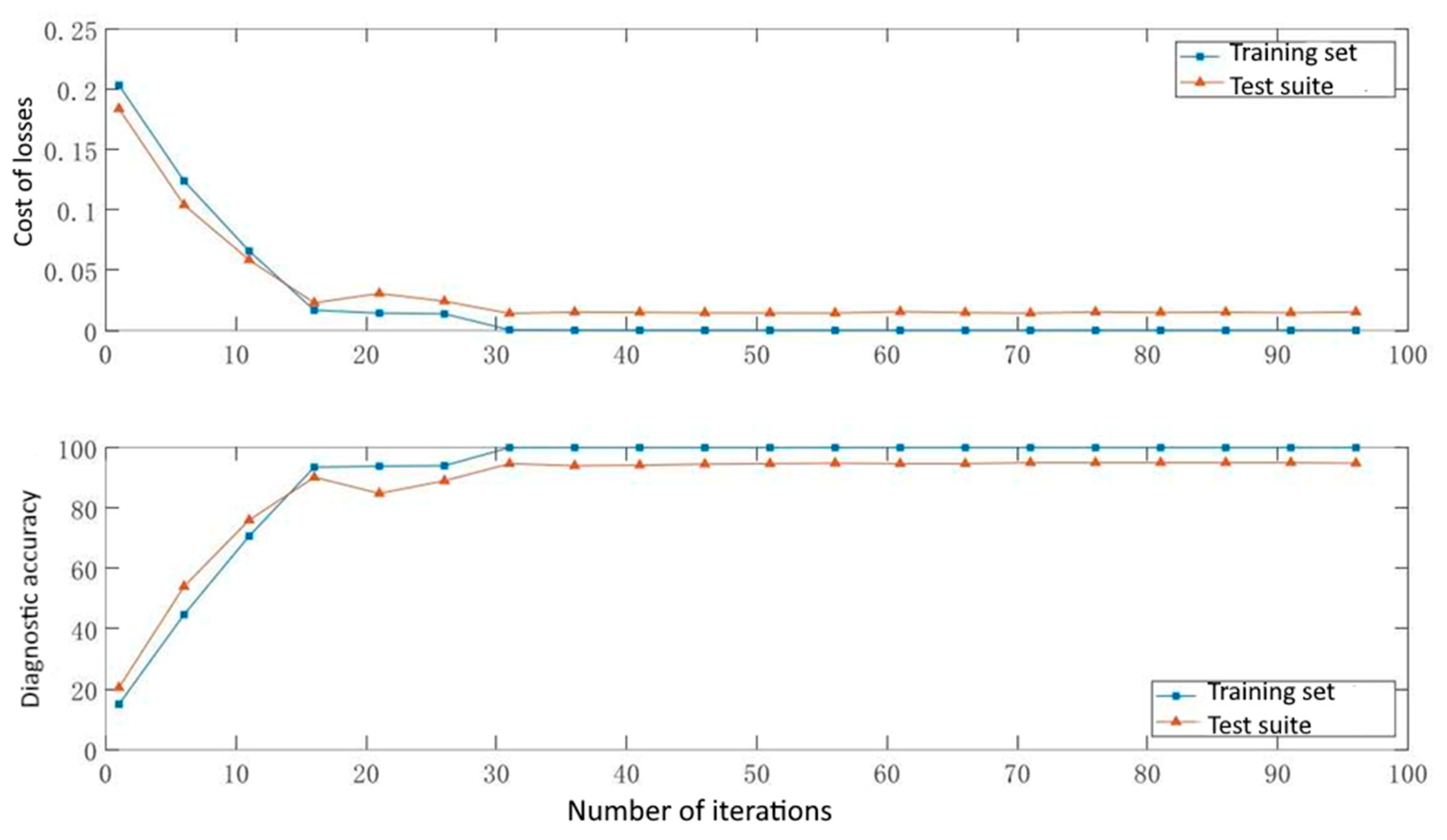
In the training phase, the training samples were used as inputs for the deep learning network, and the diagnostic results of the current network for the training set were verified by minimizing the loss function. In the testing phase, the loss function for the test set was iteratively calculated, and the fault diagnosis accuracy for the test set was determined. The convergence of losses in the training set was indicative of the network’s training status, and the diagnostic accuracy of the test set corresponded to the final diagnostic accuracy. Utilizing the 2100 rpm speed paradigm, the parameters and weights of the ResNet deep network model were initialized, the training set at 2100 rpm speed was employed to train the model, and the test set at the same speed was fed into the network for prediction and diagnosis inference. The loss function curves of the training and testing phases, along with the diagnostic accuracy of the model.

As demonstrated in Figure 11, the loss function of the training set exhibited convergence after the 31st iteration, the network loss approached zero, and the validation effect of the training set attained 100%. Meanwhile, the network loss of the test set demonstrated stability, and the diagnosis accuracy attained 95.17% following a minor fluctuation, i.e., the accuracy of the selected ResNet deep learning-based motor fault diagnosis model for faults at 2100 rpm reached 95.17%. In light of the aforementioned conditions, the ultimate classification results obtained from the confusion matrix are illustrated in Figure 12. The horizontal axis represents the actual sample label, while the vertical axis denotes the predicted label.

As demonstrated in Figure 12, the deep learning model successfully identified four distinct motor states: normal, bus break fault, eccentric fault, and inter-turn short-circuit. For bearing faults, there were very few erroneous examples, and for stator winding unbalance faults, out of 100 examples, only 72 were evaluated correctly, of which 27 were misdiagnosed as bearing faults.

In the field of deep learning, the evaluation metrics employed for multi-classification fault diagnosis models encompass Micro-F1 micro-averaging and Macro-F1 macro-averaging, along with accuracy ratio and confusion matrix. In the former, the Micro-F1 value is calculated based on the total accuracy and recall scores for all categories, while in the latter, the total Macro-F1 value is calculated by averaging the F1-score values for each category. For instance, when considering the 2100 rpm diagnosis, it is first necessary to calculate the accuracy factor P and the memorization factor R for each category. The formulae for these can be found below (Figure 13). Confusion matrix of ResNet-based deep network model results at 2100 rpm shown in the Figure 14.

$$P={\displaystyle \frac{TP}{TP+FP}},$$

(11)

$$R={\displaystyle \frac{TP}{TP+FN}},$$

(12)

where TP is true positive, meaning ‘predicted positive, actual positive’; FP is false positive, meaning ‘predicted positive, actual negative’; and FN is false negative, meaning ‘predicted negative, actual positive’. The F1-score, F1, can be calculated from precision and recall, and the formula is as follows.

$$F_1={\displaystyle \frac{2}{\frac{1}{P}+\frac{1}{R}}}={\displaystyle \frac{2\times P\times R}{P+R}},$$

(13)

As indicated by the definition, Micro-F1 is calculated by taking into account the number of instances belonging to each category in the sample. This calculation method is appropriate for unbalanced samples and also has an impact on classes with large sample sizes. In contrast, Macro-F1 considers each category equally and is influenced by the accuracy and recall rates for different categories. As demonstrated in

Table 3. Values of deep learning model evaluation index at 2100 rpm.

Refusal Category	TP	FP	FN	P	R	F1
0	100	0	0	100%	100%	1
1	100	0	0	100%	100%	1
2	100	1	0	99%	100%	0.995
3	100	0	0	100%	100%	1
4	72	1	28	99%	72%	0.8324
5	99	27	1	79%	99%	0.8761
Overall indicators	571	29	29	95%	95%	-

below, the calculation of Micro-F1 and Macro-F1 can be derived from the aforementioned equation.

The Micro-F1 and Macro-F1 values of the diagnostic model for this rotational speed were 0.9517 and 0.9506, respectively, which were greater than 0.95. This indicates that the constructed deep learning model has excellent performance in the multi-classification of motor faults and a strong generalization ability.

The ensuing discourse will address the findings from diagnostic analyses undertaken under a variety of current input strategies. The diagnostic system, incorporating a variety of current input strategies, was utilized to diagnose motor faults at three distinct speeds. The results obtained at 1500 rpm, 1800 rpm, and 2100 rpm are presented in

Table 4. Feature transfer model improved diagnosis across speed scenarios.

Migration Scenario	Original Accuracy	Accuracy After Migration	Enhancement
1500→1800 rpm	72%	89%	+17%
1800→2100 rpm	75%	92%	+17%
1500→2100 rpm	68%	85%	+17%

, which also illustrates the accuracy of the findings.

As shown in Table 3, the proposed ResNet model achieved a 100% recognition rate (F1 = 1) for high signal-to-noise ratio faults (rotor bar breakage and air gap eccentricity) at 2100 rpm, but it had low sensitivity to harmonic overlap faults (winding imbalance; F1 = 0.8324), primarily due to the coupling of its low-frequency features (Equation (5)) with bearing fault harmonics (Equation (8)) in the <500 Hz frequency band. Transfer learning significantly improved cross-condition generalization. When knowledge from the source domain (1500 rpm) was transferred to the target domain (1800 rpm), the bearing fault recognition accuracy improved from 72% to 89% (compare

Table 5. Results of motor fault diagnosis based on deep learning at different input current values.

Current Input Strategy	1500 rpm	1800 rpm	2100 rpm
Three-phase current	94.17%	95.00%	95.17%
Single-phase current (A/B/C)	92.50%	95.50%	94.50%
Three-phase current + single-phase current (A/B/C)	94.67%	95.33%	95.83%

), demonstrating that the feature alignment mechanism effectively decoupled distribution shifts caused by speed differences.

As demonstrated in Table 5, the diagnostic efficacy of the diagnostic network at 2100 rpm was generally superior to that of the other two conditions, suggesting that the motor fault characteristics were more pronounced at 2100 rpm. When comparing the circuits with different current strategies, the diagnostic accuracy when using three-phase currents and single-phase currents as inputs for different deep learning networks was higher than that when using single-phase currents as inputs. However, the difference in the diagnostic results of the former two was not significant. The result of the diagnostic process was 95.83%, which was achieved at 2100 rpm, thus meeting the requirements for the actual fault diagnosis. The specific diagnostic results are shown in Table 5, which presents the number of samples with correct prediction results out of 100 samples for each condition.

As illustrated in

Table 6. Diagnostic results with different current input strategies at 2100 rpm.

Fault Type	Three-Phase Current	Single-Phase Current (A/B/C)	Three-Phase Current + Single-Phase Current (A/B/C)
0	100	100	100
1	100	100	100
2	100	99	100
3	100	100	100
4	72	71	76
5	99	97	99
Average precision	95.17%	94.50%	95.83%

, it is evident that contemporary input strategies demonstrated superiority in differentiating normal motor conditions, jumper faults, and short-circuits between stator windings. In addition, three-phase and single-phase currents could be effectively differentiated during the diagnosis of air gap eccentricity faults and bearing faults, respectively, by employing a deep learning network. Despite the enhancement in the diagnostic accuracy of stator windings, the occurrence of misdiagnosis persists. For stator windings, although the diagnostic accuracy was improved, misdiagnoses still occurred. With regard to winding imbalance faults, the optimal diagnostic outcome was 100 samples, of which 24 were misdiagnosed, and 22 of these were predicted to be bearing faults.

The following study will compare and contrast the diagnostic results of machine learning and deep learning. In the context of the machine learning diagnostic process, it is noteworthy that the source signal feature extraction and Park’s fusion current feature extraction are analogous to the deep single-phase and three-phase current feature extraction in the current input strategy 3 of deep learning. Consequently, the outcomes observed in this condition can be utilized to directly compare the motor fault diagnosis results of machine learning and deep learning. The results of the comparison are summarized in Table 6.

As demonstrated in

Table 7. Comparison of diagnostic results between traditional machine learning and deep learning models.

	1500 rpm	1800 rpm	2100 rpm
Traditional machine learning	92.17%	92.67%	93.83%
Deep learning	95.17%	96.33%	96.83%

, the impact of conventional machine learning and deep learning was analogous across the three speeds, with an enhancement in diagnostic accuracy as the nominal speed was attained. The experiments showed that the model performed best at a speed of 2100 rpm (with an accuracy rate of 95.83%) due to the significant increase in the amplitude of fault feature frequencies at higher speeds (e.g., the rotor bar breakage feature frequency f bb ∝sf 1 increased with speed), while at 1500 rpm, the misdiagnosis rate for winding imbalance faults was relatively high (24%), primarily because the harmonic components of this fault overlapped with those of bearing faults in the low-frequency range. However, the ResNet deep network model was developed to circumvent this inherent limitation. Consequently, the ResNet deep network demonstrates considerable promise for practical applications in the diagnosis of faults in electrical machines.

4. Conclusions

Induction motors find application in a variety of industrial contexts, and the safe operation of these motors is of paramount importance in ensuring the stability of the entire system. However, due to frequent start-up and shutdown and long-term use, the probability of faults increases, thus rendering fault diagnosis and condition detection of induction motors of great importance. The advent of diagnostic technology and artificial intelligence has led to the widespread utilization of the latter as a sophisticated tool for the identification of faults in various equipment. The present paper took a squirrel cage induction motor as the object of study. It analyzed the current situation of motor fault diagnosis and the problems faced by it. It also investigated a state recognition method for the induction motor under variable operating conditions based on deep transfer learning theory. Furthermore, it studied the effect of applying multiple-source information theory to induction motor diagnosis.

This paper presented an analysis of the causes of various faults and characteristic fault frequencies in engines. A simulation model of motors was constructed, and the fault occurrence of motors in an ideal condition was analyzed using the fast Fourier transform (FFT) and Park’s extended vector method. A simulation bench of a real induction motor was constructed, and the current and vibration signals of motors in six different states were collected. Subsequently, the deep learning theory was generalized, and a deep network based on ResNet was considered the primary tool for motor state classification. In this paper, the fact that several residual modules can reduce the complexity of training the network was exploited.

It is evident that conventional signal analysis and machine learning methodologies necessitate professional expertise for the extraction of multiple time–frequency statistical features that can characterize fault information. The proposed methodology is an innovative approach to fault diagnosis for electric motors, utilizing a deep residual network. It has been demonstrated that a three-phase current carries different information, and as a result, several three-phase current injection strategies have been developed. These strategies are then used in conjunction with a deep ResNet-based network for the purpose of deep feature extraction and identification of state classification. Furthermore, a ResNet-based deep network has been constructed for motor state classification, which is then utilized for the extraction of deep features and the identification of state classification. Consequently, an engine fault diagnosis model was constructed utilizing ResNet deep learning. The experimental findings demonstrate that the accuracy of three-phase current and single-phase current data entry in the multi-branch ResNet deep learning network for feature extraction and association is superior to that of alternative strategies. Furthermore, the diagnostic accuracies at three speeds were 94.67%, 95.33%, and 95.83%, respectively, thereby validating the efficacy of deep learning for motor fault diagnosis.

The theoretical underpinnings of deep learning were presented as a solution to the issue of the low diagnostic accuracy of ResNet-based deep learning diagnostic models under variable operating conditions. Consequently, two models for diagnosing engine faults were constructed, based on parameter migration and feature migration, for variable operating conditions. The parameter migration model comprises the following steps: firstly, the shallow parameters of the ResNet-based deep network trained in the source region are fed into the target ResNet model; secondly, the shallow parameters of the target ResNet model are frozen; and thirdly, the fine-tuning samples are used to fine-tune the target ResNet model for fault diagnosis in the test set in the target region. The feature migration model utilizes the source and training data of the target region, which are concurrently fed into the deep ResNet network with shared parameters. The employment of JVM serves to enhance the accuracy of the feature migration model in the target domain. The feature migration model utilizes the source and training data of the target region, which are concurrently fed into the deep ResNet network with shared parameters. The model employs the JMMD distance metric to adapt the spatial distribution of features for the classification of faults in the test data of the target region. The experimental findings demonstrate that the feature migration model exhibits superior efficacy in the diagnosis of engine faults at varying speeds, with diagnostic accuracies of 92.17%, 88%, and 95.17% under the three operating conditions. These enhancements in diagnostic accuracy were 19.84%, 24.5%, and 14.5% higher than that of the model without migration, respectively. In order to verify the feasibility of this method, it will be deployed and validated in the main ventilation system of a coal mine in the future.