A Hybrid Symmetry Strategy Improved Binary Planet Optimization Algorithm with Theoretical Interpretability for the 0-1 Knapsack Problem

Abstract

The Planet Optimization Algorithm (POA) is a meta-heuristic inspired by celestial mechanics, drawing on Newtonian gravitational principles to simulate planetary dynamics in optimization search spaces. While the POA demonstrates a strong performance in continuous domains, we propose an Improved Binary Planet Optimization Algorithm (IBPOA) tailored to the classical 0-1 knapsack problem (0-1 KP). Building upon the POA, the IBPOA introduces a novel improved transfer function (ITF) and a greedy repair operator (GRO). Unlike general binarization methods, the ITF integrates theoretical foundations from branch-and-bound (B&B) and reduction algorithms, reducing the search space while guaranteeing optimal solutions. This improvement is strengthened further through the incorporation of the GRO, which significantly improves the searching capability. Extensive computational experiments on large-scale instances demonstrate the IBPOA’s effectiveness for the 0-1 KP, showing a superior performance in its convergence rate, population diversity, and exploration–exploitation balance. The results from 30 independent runs confirm that the IBPOA consistently obtains the optimal solutions across all 15 benchmark instances, spanning three categories. Wilcoxon’s rank-sum tests against seven state-of-the-art algorithms reveal that the IBPOA significantly outperforms all competitors $(p<0.05)$, though it is occasionally matched in its solution quality by the binary reptile search algorithm (BinRSA). Crucially, the IBPOA achieves solutions 4.16 times faster than the BinRSA on average, establishing an optimal balance between solution quality and computational efficiency.

1. Introduction

The 0-1 knapsack problem (0-1 KP) [1], a canonical NP-hard problem [2,3,4], and its various variants [5] remain widely studied despite the absence of polynomial time exact algorithms. The simplicity of its formulation and the flexibility of its variants for modeling diverse real-world constraints have ensured its relevance across applications such as portfolio selection [6,7], rectilinear building frames [8], complex planning and scheduling [9], and picking–packing and delivery problems [10]. High-quality solutions to these problems can yield significant economic benefits and profits, driving sustained research interest in NP-hard problem variants, particularly the 0-1 KP. The mathematical formulation of the 0-1 KP is as follows:

Definition 1

([1]). Take a set $N=\{1,\dots ,n\}$ of n items where each item j has a profit $p_j>0$ and a weight $w_j>0$. The 0-1 KP aims to select a subset of N that maximizes the total profit while ensuring the total weight does not exceed the knapsack’s capacity C. The problem can be formulated as follows.

$$\begin{array}{c}\hfill maxf\left(\mathit{X}\right)=\sum _{j=1}^n{x}_j{p}_j,\end{array}$$

(1)

s.t.

$$\begin{array}{c}\hfill g\left(\mathit{X}\right)=\sum _{j=1}^n{x}_j{w}_j\le C,\end{array}$$

(2)

$$\begin{array}{c}\hfill x_j\in \{0,1\},\end{array}$$

(3)

where $x_j=1$ indicates the selection of the j-th item, and $x_j=0$ indicates non-selection. The objective function (1) of the model aims to maximize the total profit of the selected items. Constraint (2) enforces the total weight of selected items not exceeding the knapsack’s capacity C, while (3) specifies binary decision variables. To exclude trivial solutions, we assume ${\displaystyle \sum _{j=1}^n}{w}_j>C$ and $w_j\le C$ for all $j\in N$. Additionally, for clarity in the subsequent analysis, items are sorted such that ${\displaystyle \frac{p_1}{w_1}}\ge {\displaystyle \frac{p_2}{w_2}}\ge \cdots \ge {\displaystyle \frac{p_n}{w_n}}$.

Since only exact algorithms with non-polynomial time complexity exist for the large-scale 0-1 KP, such as dynamic programming (DP) [11] and branch-and-bound (B&B) [12,13], meta-heuristic algorithms (MAs), particularly genetic algorithms (GAs) [14], have become the dominant approach.

The increasing diversity of MAs has demonstrated that the framework of multiple sub-swarms effectively enhances the search performance. This framework has been widely adopted by prominent algorithms such as Gray Wolf Optimization (GWO) [15], Dynamic Mentoring and Self-Regulation-Based Particle Swarm Optimization (DMeSR-PSO) [16], and Bee Colony Optimization (BCO) [17]. While sub-swarm mechanisms improve the algorithmic performance, their effectiveness is highly sensitive to the parameter settings during partitioning. Therefore, partitioning parameter-free MAs with a robust performance and well-designed mechanisms represents a valuable research direction.

To address parameter tune in sub-swarm partitioning, Thanh et al. [18] proposed the Planet Optimization Algorithm (POA), inspired by celestial mechanics. The POA designates the global best solution $g_{\mathrm{best}}$ as the Sun, with the other solutions (planets) orbiting it, while distant solutions experience weaker attraction, maintaining proximity to the current positions. This gravitational mechanism achieves parameter-free synergy between local and global search, demonstrating an excellent algorithmic performance within continuous search spaces, including scenarios such as 23 well-known test functions, 38 IEEE CEC benchmark test functions (CEC2017, CEC2019), and 3 real engineering problems (tension/compression spring design, welded beam design, and pressure vessel design).

The POA partitions individuals into multiple sub-swarms through a simple mechanism that effectively maintains the population diversity without empirical parameter dependence. This approach provides a valuable framework for solving NP-hard problems. However, extending this framework to discrete spaces requires structural modifications via discretization strategies. To address this, we propose an Improved Binary Planet Optimization Algorithm (IBPOA) for the 0-1 KP. Preserving the POA’s sub-swarm mechanism, the IBPOA introduces a distinct discretization approach. We propose an improved transfer function (ITF) that incorporates Yang’s reduction algorithm [19], as an alternative to the standard sigmoid-based binarization strategies. The ITF modifies the sigmoid transfer function by leveraging B&B theory. This modification symmetrically adjusts the selection probabilities relative to the hyperplane formed by the break item (also called the split item) and the origin. The magnitude of the adjustment scales proportionally to an item’s distance from this hyperplane. This enhancement simultaneously prunes the search space, accelerates the convergence, and preserves global optimality guarantees. The main contributions of this paper are

• Practically, the IBPOA outperforms other methods from the literature [20] for the 0-1 KP while providing an extensible POA-based framework for related NP-hard problems. Its sub-swarm mechanism further offers transferable population structures for other MAs.
• Enhancement of the ITF operator embeds B&B theory with rigorous interpretability. Its parameters self-adapt to problem instances, boosting the search capabilities while ensuring the existence of an optimal solution.
• Computational evaluations on 15 literature benchmarks [20] confirm the IBPOA’s superiority in its convergence acceleration, diversity preservation, and exploration–exploitation equilibrium, with seamless adaptability to 0-1 KP variants.

The remainder of this paper is organized as follows. Section 1 reviews related work on the IBPOA. Section 2 details the IBPOA framework and its enhancements over the original POA. Section 3 evaluates the computational performance against that of comparison algorithms from the literature. Concluding remarks and future research directions are presented in the final section.

2. The Literature Review

With the growing diversity of MAs, numerous algorithms now exist for solving the 0-1 KP. Based on encoding schemes, these approaches fall into two primary categories: binary encoding and real encoding [21], such as Hybrid Rice Optimization (HRO) [22], the Binary Artificial Jellyfish Search Algorithm (Bin-AJS) [23], the Binary Marine Predators Algorithm (BMPA) [24], and the Monogamous Pairs Genetic Algorithm (MPGA) [25]. Binary-encoded algorithms operate on bit-string representations directly, whereas real-encoded algorithms obtain 0-1 KP solutions by converting continuous solutions via transfer functions (TFs). Concurrently, researchers are attempting to explore novel encoding schemes to enhance the algorithmic performance. Complex-valued encoding represents decision variables using complex numbers, leveraging both real and imaginary components. This approach increases the information capacity and improves the population diversity. During decoding, these algorithms first convert complex values into real numbers via the L2-norm, assigning the sign bit based on the phase angle. The resulting real values are then mapped to binary solutions employing TFs (e.g., the sigmoid function). A few complex-valued encoding algorithms have been developed for the 0-1 KP, such as the Complex-Valued Bat Algorithm (CPBA) [26] and Complex-valued Wind Driven Optimization (CWDO) [27]. Additionally, some MAs utilize less scalable encoding schemes for the 0-1 KP, including Quantum-Inspired Social Evolution (QSE) [28], Quantum-Inspired Differential Evolution with Gray Wolf Optimizer (QDGWO) [29], and the Modified Discrete Shuffled Frog Leaping Algorithm (MDSFL) [30].

As a representative of MAs, Particle Swarm Optimization (PSO) [31] was first proposed by Kennedy and Eberhart for continuous optimization. Two years later, they introduced Binary Particle Swarm Optimization (BPSO) [32] to solve discrete optimization problems such as the 0-1 KP. As of 2023, incomplete statistics indicated that over 540 MAs exist [33], among which more than 57 are inspired by or exhibit iterative mechanisms similar to PSO [34]. Examples include widely applied algorithms like the Bee Colony Optimization [17], the Sine Cosine Algorithm [35,36], and the Moth-Flame Optimization Algorithm [37]. Thus, high-performance improvement operators not only enhance PSO’s problem-solving efficacy but also significantly benefit its variants. Research on such operators is therefore critically important.

During the discretization of PSO and its variants, these algorithms typically employ sigmoid functions to map continuous-space solutions into discrete/binary spaces. This approach causes significant position fluctuations when particle velocities approach zero, resulting in compromised local search capabilities. To address this issue, researchers have developed improvements primarily through two approaches:

On the one hand, one research direction involves modifying TFs by replacing sigmoid functions with alternative formulations [20,38,39]. Mirjalili and Lewis developed the S-shaped transfer function by scaling the original sigmoid function with a coefficient $\alpha$. To address the position oscillation issue near zero velocity inherent in S-shaped functions, they subsequently introduced a V-shaped transfer function based on $tanhx$ and its variants [38]. Following similar principles, Mirjalili et al. proposed a U-shaped transfer function using the exponents ${\left|v\right|}^k$ ($k>1$), while He et al. created a taper-shaped transfer function with ${\left|v\right|}^k$ ($0<k<1$) [39,40]. Separately, Guo et al. derived a Z-shaped transfer function from $\sqrt{1-{\alpha }^{\beta }}$ where $\alpha \in {\mathbb{R}}^{+}$ and $\beta$ denotes the particle velocity [41]. Empirical studies confirm that the TF’s performance varies significantly across problem domains, making its careful selection essential for algorithmic optimization.

On the other hand, besides sharing common drawbacks like a lack of a theoretical foundation with other MAs, PSO inherently exhibits relatively weak local search capabilities due to the insufficient synergy among particles caused by its iterative update rules [42,43,44]. To address this, researchers have proposed various improvement strategies, with multi-sub-swarm structures representing a significant direction. Kennedy and Mendes incorporated topological structures inspired by simulated annealing algorithms, modifying particle movement toward the global best and personal best solutions to target neighboring local best solutions instead. This approach substantially enhanced the population diversity [45]. Similarly, Ye et al. partitioned particles into sub-swarms and redirected particle updates toward the personal best solutions and the arithmetic mean of all local best solutions [46]. Notably, while well-designed topologies can significantly improve PSO’s performance and avoid local optima, selecting the appropriate structures remains challenging [43]. As an alternative to topology selection, Tanweer et al. classified particles into mentor, mentee, and independent learner groups based on the fitness differences and the Euclidean distance from the global best particle, proposing DMeSR-PSO [16]. Experimental results demonstrate that DMeSR-PSO not only eliminates topology selection but also outperforms six PSO variants and five MAs on the CEC2005, CEC2011, and CEC2013 benchmark functions.

Clearly, the classification rules for different groups in DMeSR-PSO significantly influence the solution quality while being empirically parameter-dependent. Similarly, parameter tuning for sub-swarm partitioning persists in PSO variants. In this work, we preserve the parameter-free sub-swarm partitioning mechanism of the POA while introducing the IBPOA, an enhanced heuristic for the 0-1 KP. Table 1, Table 2 and Table 3 compare the IBPOA with the algorithms from [20]. To demonstrate the IBPOA’s superiority, Table 4 and Table 5 present the results of Wilcoxon’s rank-sum tests against these benchmarks, confirming that the IBPOA satisfies both the computational efficiency and accuracy requirements for the problem. Additionally, the ablation studies in Table 6 compare the proposed ITF operator against 20 transfer functions (including S-shaped [38], V-shaped [38], U-shaped [40], taper-shaped [39], and Z-shaped [41] functions), showing the ITF’s significant advantage in solving the 0-1 KP.

3. The Improved Binary Planet Optimization Algorithm (IBPOA)

This section details the IBPOA, beginning with related operators of the POA in Section 3.1. We then develop an ITF leveraging B&B theory [19] for real-to-binary encoding conversion, integrated with a greedy repair operator (GRO) for constraint handling. Section 3.4 establishes the theoretical foundations for the ITF and analyzes the implementation properties, which represent advances beyond the conventional methodologies. An analysis of the computational complexity of the IBPOA is presented in Section 3.6.

3.1. A Review of the Planet Optimization Algorithm (POA)

3.1.1. Initial Solution Generation

For an n-dimensional continuous optimization problem, let $X^t$ represent the population of the POA in the t-th generation, where $0\le t\le T$. Here, t denotes the current iteration, and T represents the maximum number of iterations. Clearly, $X^0$ is the initial solution of the algorithm. Let $x_{i,j}^t$ be the j-th variable of the i-th individual in the t-th generation. The indices satisfy the constraints $1\le j\le n$ and $1\le i\le \mathrm{pop}$, where pop is the size of the population. The initial solution of the POA can be expressed as follows.

$$\begin{array}{c}\hfill x_{i,j}^0=\mathrm{rand}\times ({\mathrm{UB}}_j-{\mathrm{LB}}_j)+{\mathrm{LB}}_j,\end{array}$$

(4)

where UB and LB are the maximum and minimum values of the j-th decision variable in the problem, respectively, and rand is a uniformly distributed random number in the range $[0,1]$. In particular, each rand value is independent of one another.

3.1.2. The Moment of the Planet

The POA introduces gravitation to guide the iterative direction of individuals. Experimental results demonstrate that the moment of gravitation becomes more effective computationally compared to gravitation itself. Similar to gravitation, the moment’s value depends on interplanetary distances and masses. In the POA, a planet’s mass is determined by its objective function value: higher values correspond to a greater mass, exerting a stronger gravitational pull. The mass $m_i$ is

$$\begin{array}{c}\hfill m_i=a^{{\displaystyle \frac{\alpha }{\alpha +minf\left(X^t\right)-f\left(X_i^t\right)+1}}},\end{array}$$

(5)

where $a=2$, $minf\left(X^t\right)$ is the minimal objective value in generation t, and

$$\begin{array}{c}\hfill \alpha =|minf\left(X^t\right)-f\left(X_{\mathrm{Sun}}^t\right)|,\end{array}$$

(6)

where $f\left(X_{\mathrm{Sun}}^t\right)$ is the Sun’s objective value, i.e., the best in generation t.

The Euclidean distance between planet i and the $\mathrm{Sun}$ is

$$\begin{array}{c}\hfill R_{i,\mathrm{Sun}}=\parallel X_i^t-X_{\mathrm{Sun}}^t\parallel =\sqrt{\sum _{j=1}^n{\left(x_{ij}^t-x_{\mathrm{Sun},j}^t\right)}^2}\end{array}$$

(7)

In the solar system, planets are primarily attracted by stellar gravity. Thus, we focus on Sun–planet interactions rather than the inter-planet gravitation. The gravitational moment between planet i and the Sun in generation t is

$$\begin{array}{c}\hfill M_i^t=\parallel \overrightarrow{F}\parallel ·R_{i,\mathrm{Sun}}=G{\displaystyle \frac{m_i{m}_{\mathrm{Sun}}}{R_{i,\mathrm{Sun}}}}\end{array}$$

(8)

where $G=1$ is the gravitational constant, and $m_{\mathrm{Sun}}$ is the Sun’s mass.

3.1.3. Global Search

During the global search, individual $X_i^t$ is updated as follows:

$$\begin{array}{c}\hfill X_i^{t+1}=X_i^t+d\times {\beta }_i\times \mathrm{rand}\times (X_{\mathrm{Sun}}^t-X_i^t),\end{array}$$

(9)

where $X_i^{t+1}$ is the updated individual of $X_i^t$, $d=1$ is a constant, $\mathrm{rand}\sim U[0,1]$, and $X_{\mathrm{Sun}}^t$ represents the Sun individual in generation t.

In (9), ${\beta }_i$ controls the maximum displacement toward the Sun during global search and is calculated as follows.

$$\begin{array}{c}\hfill {\beta }_i={\displaystyle \frac{M_i^t}{M_{max}^t}},\end{array}$$

(10)

where $M_{max}^t$ is the maximum of $M^t$. Thus, ${\beta }_i\in (0,1]$.

3.1.4. Local Search

During the local search, individual $X_i^t$ is updated as follows:

$$\begin{array}{c}\hfill X_i^{t+1}=X_i^t+c\times \mathrm{rand}\times (\gamma \times X_{\mathrm{Sun}}^t-X_i^t),\end{array}$$

(11)

where $c=c_0-t/T$ is an adaptive factor, $\mathrm{rand}\sim U[0,1]$, and $\gamma \sim \mathrm{N}(\mu ,{\sigma }^2)$, where the empirical parameters are set to $\mu =0.5$ and $\sigma =0.2$. We adopt these settings from the literature [18].

3.1.5. The Control Search Factor

The POA employs two distinct search methods. In the population of the t-th generation, the iteration strategy for an individual $X_i^t$ is determined by the distance between the planet and the Sun. The POA utilizes a parameter $R_{min}$ to choose between local and global search for each individual. Specifically, during the t-th iteration, if the distance $R_{i,\mathrm{Sun}}$ between the i-th planet and the Sun satisfies $R_{i,\mathrm{Sun}}\le R_{min}$, the algorithm applies local search to the i-th individual; otherwise, global search is employed.

The value of $R_{min}$ is crucial. As reported by Thanh et al. [18], it is defined by the following formula:

$$\begin{array}{c}\hfill R_{min}={\displaystyle \frac{{\displaystyle \sum _{j=1}^n}{({\mathrm{UB}}_j-{\mathrm{LB}}_j)}^2}{R_0}},\end{array}$$

(12)

where $R_0$ is a preset experimental value, typically set to 1000.

3.2. An Improved Transfer Function (ITF)

Section 3.1 outlined the core mechanisms of the POA. Due to its real encoding scheme, the POA is not directly applicable to discrete optimization problems such as the 0-1 KP. The sigmoid function serves as the classical transfer function for mapping continuous spaces to binary spaces and is widely adopted in PSO and its variants for discretization. Let $Y_i^t$ and $y_{ij}^t$ denote the binary counterparts of $X_i^t$ and $x_{ij}^t$ after applying the transfer function:

$$\begin{array}{c}\hfill \begin{array}{c}\hfill y_{ij}^t=\left\{\begin{array}{cc}1,\hfill & \mathrm{if}\mathrm{rand}<{\displaystyle \frac{1}{1+e^{-x_{ij}^t}}},\hfill \\ 0,\hfill & \mathrm{otherwise}.\hfill \end{array}\right.\end{array}\end{array}$$

(13)

where $\mathrm{rand}\sim U(0,1)$ is a uniformly distributed random number.

The sigmoid function maps the continuous-space solution $x_{ij}^t$ into the interval $(0,1)$. A random number rand is then used to determine the binary assignment: if $\mathrm{rand}<{\displaystyle \frac{1}{1+e^{-x_{ij}^t}}}$, $y_{ij}^t$ is assigned 1; otherwise, it is assigned 0. To enhance the search capability of the algorithm further, we propose an improved transfer function tailored to the characteristics of the 0-1 KP.

Very recently, Yang [19] adapted the improved B&B method proposed by Dey et al. [47] to solving the 0-1 KP. For a given instance $\mathcal{P}$, the method first applies a greedy strategy: items are packed in non-increasing order of their profit density (i.e., ${\displaystyle \frac{p_j}{w_j}}$) until the first item exceeds the knapsack’s capacity. This yields the break item b and the break solution ${\mathbf{X}}^{\prime }=(x_1^{\prime },\dots ,x_{b-1}^{\prime },x_b^{\prime },\dots ,x_n^{\prime })$, where $b=min\{k:{\sum }_{j=1}^k{w}_j>C\}$, $x_1^{\prime }=\cdots =x_{b-1}^{\prime }=1$ and $x_b^{\prime }=\cdots =x_n^{\prime }=0$. Next, the Dantzig upper bound $U\left(\mathcal{P}\right)$ [48] is computed via linear relaxation, $U\left(\mathcal{P}\right)={\sum }_{k=1}^{b-1}{p}_k+⌊r{p}_b/w_b⌋$, where $r=C-{\sum }_{k=1}^{b-1}{w}_k$ denotes the residual capacity. Finally, the B&B reduction phase searches for feasible solutions with objective values no less than that of the break solution $f\left(X^{\prime }\right)$.

From the literature [19], we have the following definition and theorem.

Definition 2

([19]). The item set $N_1=\{1,2,\dots ,b-1\}$, consisting of items with a higher profit density than the break item b, can be divided into m disjoint subsets, denoted as $N_1={\bigsqcup }_{\omega =1}^m{N}_{1,\omega }$. Each subset $N_{1,\omega }$ has $n_{1,\omega }$ items and can be defined as follows:

$$\begin{array}{c}\hfill N_{1,\omega }=\left\{j:⌊{\displaystyle \frac{r{p}_b}{p_j{w}_b-p_b{w}_j}}⌋+1=\omega ,{\displaystyle \frac{p_j}{w_j}}>{\displaystyle \frac{p_b}{w_b}}\right\},\end{array}$$

(14)

where r is the residual capacity. If no item satisfies the Formula (14) for a given ω ($1\le \omega \le m$), then $N_{1,\omega }=\varnothing$.

Definition 2 first constructs a hyperplane based on the coordinates of the origin and the break item (i.e., the numerical values of the item’s profit $p_j$ and weight $w_j$). Subsequently, the definition assigns a value $\omega$ to each item according to its distance from the hyperplane, with $\omega$ decreasing as the distance increases. Correspondingly, the set $N_2=\{b,b+1,\dots ,n\}$, composed of items whose profit density is less than that of the break item, satisfies the following expression.

$$\begin{array}{c}\hfill N_{2,\omega }=\left\{j:⌊{\displaystyle \frac{r{p}_b}{p_b{w}_j-p_j{w}_b}}⌋+1=\omega ,{\displaystyle \frac{p_j}{w_j}}\le {\displaystyle \frac{p_b}{w_b}}\right\}.\end{array}$$

(15)

Depending on the value of $\omega$, we have the following theorem.

Theorem 1

([19]). For each ω ($1\le \omega \le m$), let $D_{1,\omega }$ denote the set of items not packed into the optimal solution from $N_{1,\omega }$, and let $s_{1,\omega }=|D_{1,\omega }|={\displaystyle \sum _{j\in N_{1,\omega }}}|y_j-1|$. These values $s_{1,\omega }$ constitute the vector $S={\left(s_{1,\omega }\right)}_{\omega =1}^m$. Therefore, we can conclude that

$$\begin{array}{c}\hfill \sum _{\omega =1}^m{\displaystyle \frac{s_{1,\omega }}{\omega }}<1.\end{array}$$

Theorem 1 reveals that at most $\omega -1$ items in $N_{1,\omega }$ are excluded from the optimal solution. In other words, all of the items in $N_{1,1}$ are selected in the optimal solution. At most one item in $N_{1,2}$ is excluded, and so on. The smaller an item’s $\omega$-value in $N_{1,\omega }$, the higher the item’s likelihood of optimal inclusion.

Conversely, at most $\omega -1$ items in $N_{2,\omega }$ are included in the optimal solution. Specifically, no items in $N_{2,1}$ are selected. Up to one item in $N_{2,2}$ may be chosen, and so on. Smaller $\omega$ values for items in $N_{2,\omega }$ correlate with reduced selection probabilities. To streamline the subsequent discussion, we denote the $\omega$-value associated with each decision variable as $\varpi$, which is computed as follows.

$$\begin{array}{c}\hfill \begin{array}{c}\hfill {\varpi }_j=\left\{\begin{array}{cc}\lfloor {\displaystyle \frac{r{p}_b}{p_j{w}_b-p_b{w}_j}}\rfloor +1,\hfill & \mathrm{if}{e}_j>e_b,\hfill \\ \lfloor {\displaystyle \frac{r{p}_b}{p_b{w}_j-p_j{w}_b}}\rfloor +1,\hfill & \mathrm{if}{e}_j<e_b,\hfill \\ \infty ,\hfill & \mathrm{otherwise}.\hfill \end{array}\right.\end{array}\end{array}$$

(16)

Building on the formula above, we propose an improved transfer function (ITF). The ITF partitions the set of items into two subsets based on the break item b’s profit density. For each item, the ITF assigns a distance-weighted value ${\displaystyle \frac{1}{{\varpi }_j}}$ using the item’s distance to the hyperplane formed by the break item and the origin. For items with a profit density exceeding the break item, the ITF increases the probability of setting $y_{ij}^t=1$; symmetrically, for items with a profit density below the break item, it increases the probability of setting $y_{ij}^t=0$. The ITF is formally defined as follows:

$$\begin{array}{c}\hfill \begin{array}{c}\hfill y_{ij}^t=\left\{\begin{array}{cc}1,\hfill & \mathrm{if}\mathrm{rand}<{\displaystyle \frac{1}{1+e^{-x_{ij}^t}}}+{\displaystyle \frac{1}{{\varpi }_j}},\mathrm{and}{e}_j\ge e_b\hfill \\ 1,\hfill & \mathrm{if}\mathrm{rand}<{\displaystyle \frac{1}{1+e^{-x_{ij}^t}}}-{\displaystyle \frac{1}{{\varpi }_j}},\mathrm{and}{e}_j<e_b\hfill \\ 0,\hfill & \mathrm{otherwise},\hfill \end{array}\right.\end{array}\end{array}$$

(17)

where $\mathrm{rand}\sim U(0,1)$.

Building on Formula (13), the ITF in Formula (17) partitions the item set N into two subsets $N_1$ and $N_2$ based on the break item b’s profit density. The value ${\varpi }_j$ for the j-th item is determined via Formula (14) for $N_1$ and Formula (15) for $N_2$, affecting $y_{ij}^t$. To illustrate the refined transfer function, consider the items in $N_{1,1}$. For any $j\in N_{1,1}$, the item is guaranteed inclusion in the optimal solution. Observe that ${\displaystyle \frac{1}{1+e^{-x_{ij}^t}}}+{\displaystyle \frac{1}{{\varpi }_j}}>1$, ensuring $y_{ij}^t=1$ for all $x_{ij}^t$. As ${\varpi }_j$ increases, ${\displaystyle \frac{1}{{\varpi }_j}}$ decreases monotonically, reflecting the item’s hyperplane proximity. Consequently, the items in $N_{1,\omega }$ exhibit a diminishing selection certainty, leading the algorithm to prioritize searching for these variables. Conversely, for the items in $N_{2,1}$, ${\displaystyle \frac{1}{1+e^{-x_{ij}^t}}}-{\displaystyle \frac{1}{{\varpi }_j}}<0$, forcing $y_{ij}^t=0$ for all $j\in N_{2,1}$. Here, smaller ${\varpi }_j$ values correspond to stronger guarantees of exclusion from the optimal solution.

Therefore, the ITF prioritizes exploring decision variables near the hyperplane defined by the origin and the break item b. By reducing the number of variables definitively included in or excluded from the optimal solution, the algorithm maintains its search capability while accelerating the convergence.

3.3. An Example for the ITF

To facilitate discussion, we introduce the following example to illustrate the working principle of the ITF.

Example 1.

Consider a 0-1 KP instance with $C=115$ and $n=4$ items. The profit and weight of each item are given in the following table, where the break item is the third item ($p_3=73,w_3=70$). Parameter ϖ is computed utilizing Formula (16).

$\mathit{j}$	1	2	3	4
$p_j$	90	36	73	16
$w_j$	13	33	70	86
${\varpi }_j$	1	46	∞	1

To demonstrate the ITF workflow, consider a real encoding individual ${\mathbf{X}}_i^t=(-2.9,-3.1,1.1,0.9)$ and the random variable rand. For illustration, we fix $\mathrm{rand}=0.5$. We denote the standard sigmoid (13) and the improved transfer function (17) as $\mathrm{Sig}\left(X_i^t\right)$ and $\mathrm{ITF}\left(X_i^t\right)$, respectively; the transformation proceeds as follows.

As illustrated in Figure 1, the binary solution $Y_i^t$ obtained by processing the real-encoded individual $X_i^t$ through the traditional sigmoid transfer function yields a total profit of 89 and a total weight of 156 (exceeding the knapsack’s capacity of 115), constituting an infeasible solution. In contrast, the binary solution $Y_i^t$ generated via the ITF achieves a total profit of 163 and a weight of 83, matching the optimal solution for Example 1. This demonstrates that even for real encoding individuals producing significantly underperforming solutions under sigmoid-based transformation, the ITF mechanism robustly maintains the solution quality while generating superior solutions.

3.4. The Theoretical Analysis of the ITF

In previous studies, researchers evaluating novel meta-heuristic algorithms typically conducted simulations on benchmark instances, employing computational results to demonstrate the effectiveness of the improvements. However, since meta-heuristic algorithms are stochastic, the results of individual simulation runs are not unique, rendering computational comparisons alone insufficient to robustly justify algorithmic enhancements. Unlike conventional approaches, the ITF is derived from the theoretical framework of B&B, providing stronger analytical guarantees.

Given an instance of the 0-1 KP composed of a set N of n items, the discretization strategies in previous research have first mapped the individual encoding $X_i^t$ from the continuous search space ${\mathbb{R}}^n$ to the probability space $\mathfrak{P}={(0,1)}^n$ via the sigmoid function and acquired the corresponding probability vector $Z_i^t$. Then, a binary encoding $Y_i^t\in {\{0,1\}}^n$ is generated by comparing each value in the probability vector $Z_i^t$ with a randomly sampled number. The space mapping relationship is

$$\begin{array}{c}\hfill {\mathbb{R}}^n\to {(0,1)}^n\to {\{0,1\}}^n.\end{array}$$

From Formula (17), the ITF narrows the probability mapping space for the j-th decision variable to either $\left({\displaystyle \frac{1}{{\varpi }_j}},1\right)$ or $\left(0,1-{\displaystyle \frac{1}{{\varpi }_j}}\right)$, depending on the value of ${\varpi }_j$. This contrasts with traditional TFs, which use the full interval $(0,1)$. We denote the reduced probability mapping space of the ITF as ${\mathfrak{P}}^{\prime }$. To quantify this reduction, we employ the Lebesgue Measure for theoretical comparison. The measure of the probability mapping space for the traditional transfer function is $\mu \left(\mathfrak{P}\right)=1$, whereas the measure per dimension for the ITF is $1-{\displaystyle \frac{1}{{\varpi }_j}}$. Thus, the total measure of ${\mathfrak{P}}^{\prime }$ is

$$\begin{array}{c}\hfill \mu \left({\mathfrak{P}}^{\prime }\right)=\prod _{j=1}^n\left(1-{\displaystyle \frac{1}{{\varpi }_j}}\right)\end{array}$$

(18)

Clearly, $\mu \left({\mathfrak{P}}^{\prime }\right)$ is less than $\mu \left(\mathfrak{P}\right)$. A reduced probability mapping space implies that the improved algorithm can eliminate unproductive search regions, thereby enhancing the search capability. Notably, the design of the ITF based on Theorem 1 guarantees that the optimal solutions remain within the search space. Furthermore, unlike parameter-dependent reduction methods, the ITF requires no additional parameter tuning, improving its generalization capability.

3.5. The Greedy Repair Operator (GRO)

Although the ITF significantly improves the search efficiency, solutions generated during iterations for constrained optimization problems often suffer from two common issues: constraint violations or suboptimal solutions that fail to saturate the constraint bounds. To address this challenge, meta-heuristic algorithms typically incorporate constraint-handling mechanisms. The current mainstream approaches include penalty function methods and repair strategies [20,49,50]. For the 0-1 KP, this study adopts a widely used greedy repair operator (GRO) to refine the solutions generated during iterations.

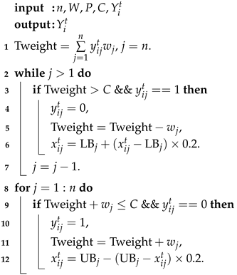
Given an individual $Y_i^t$ processed by the ITF, the GRO operates in two phases: (1) repairing the infeasibility by eliminating items in ascending profit density order and (2) optimizing the feasibility by tentatively adding items in descending profit density order. We assume the item order reflects a non-increasing profit density (i.e., $p_j/w_j\ge p_{j+1}/w_{j+1}$). The GRO procedure is formalized in Algorithm 1.

Algorithm 1: Greedy repair operator (GRO)

Algorithm 1 first repairs infeasible solutions through Steps 2–7. Subsequently, Steps 8–12 refine the solution via greedy optimization. The operations maintain a time complexity of $O\left(n\right)$. Compared to the original POA, the IBPOA introduces only two additions: the ITF and the GRO. Crucially, both components exhibit a lower time complexity than that of the core POA framework, preserving the algorithm’s computational efficiency.

Notably, since the GRO operates directly on $Y_i^t$, it may induce encoding–decoding disruption. This phenomenon stems from the algorithm’s dual-space operation (e.g., continuous and binary encodings): if the GRO modifies $Y_i^t$ without synchronously updating $X_i^t$, the search direction diverges from the actual optimization trajectory in the solution space. To mitigate this, the GRO adjusts $X_i^t$ for variables altered in $Y_i^t$ (via Lines 6 and 12). Specifically, when $y_{ij}^t$ changes from 1 to 0, the corresponding $x_{ij}^t$ is repositioned to 20% of its original distance from ${\mathrm{LB}}_j$, where the 0.2 scaling factor is an empirical value determined through experimentation. Conversely, when $y_{ij}^t$ changes from 0 to 1, $x_{ij}^t$ is similarly repositioned to 20% of its original distance from ${\mathrm{UB}}_j$.

3.6. A Complexity Analysis of the IBPOA

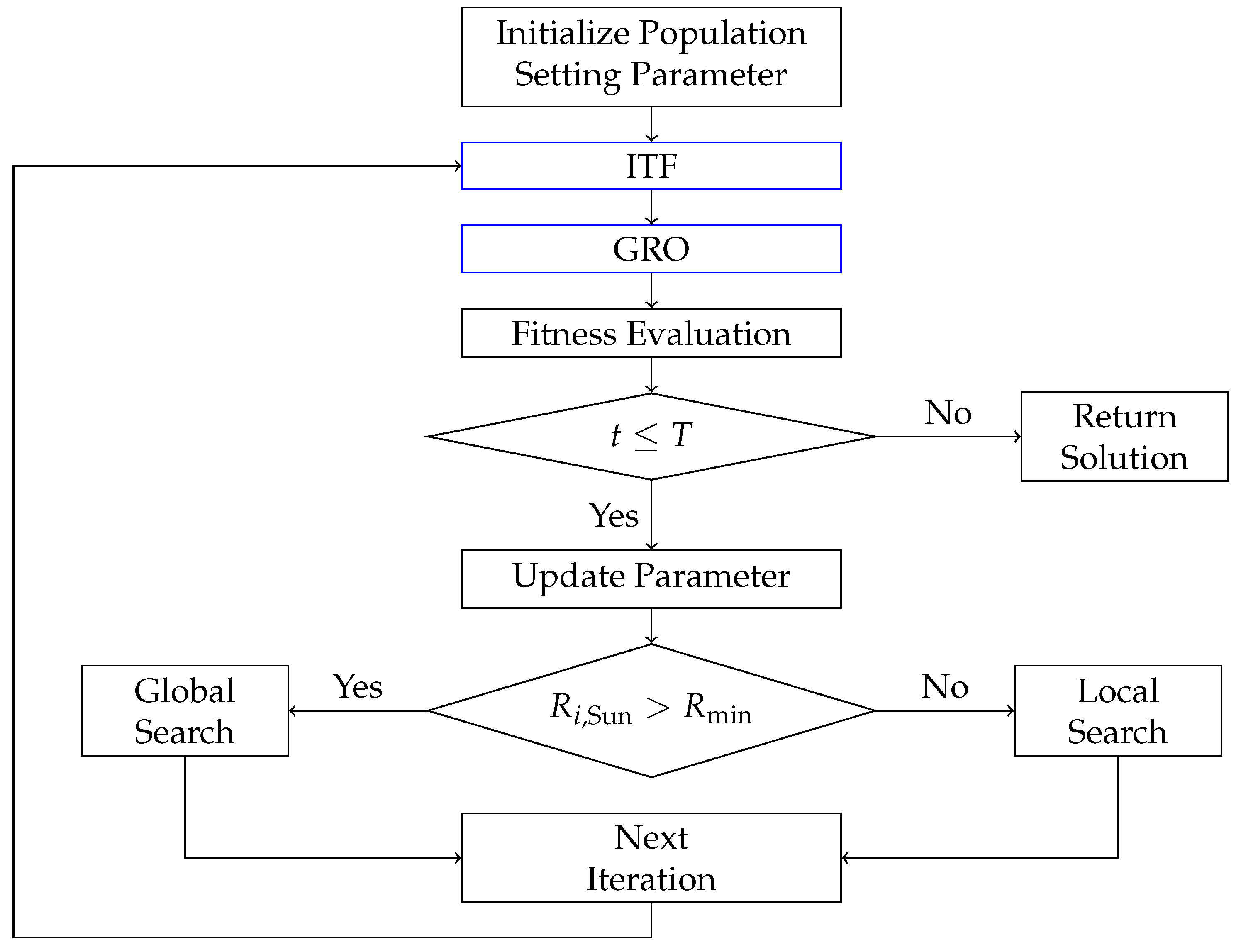
Building on the POA framework, the IBPOA introduces a greedy repair operator (GRO) to boost the search performance further. The workflow is illustrated in Figure 2, where black boxes denote the original POA operations and blue boxes highlight IBPOA-specific additions.

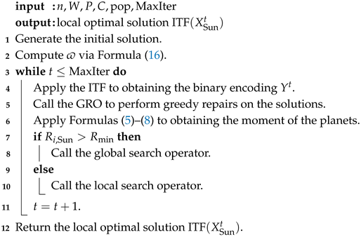
The computational complexity of the IBPOA is analyzed in this subsection. Pseudo-code appears in Algorithm 2, with the population size pop and maximum iterations MaxIter.

In the IBPOA, the time complexity of generating the initial solution is $O(\mathrm{pop}\times n)$ (Algorithm 2, Line 1). The computational complexity of computing $\varpi$ is $O\left(n\right)$ (Algorithm 2, Line 2). Within the loop, the time complexity of the $\mathrm{ITF}$ is $O(\mathrm{pop}\times n)$ (Algorithm 2, Line 4), and that of the $\mathrm{GRO}$ is $O(\mathrm{pop}\times n)$ (Algorithm 2, Line 5). For the planetary moment computations, the time complexities of Formulas (5) to (7) are all $O(\mathrm{pop}\times n)$, while that of Formula (8) is $O\left(\mathrm{pop}\right)$ (Algorithm 2, Line 6). The time complexities of the global search operator and the local search operator are both $O(\mathrm{pop}\times n)$. Thus, the time complexity of the IBPOA is $O(\mathrm{MaxIter}\times \mathrm{pop}\times n)$.

To facilitate reproducibility and future research, the implementation of the IBPOA is publicly available at https://github.com/zhugemutian/Improved-Binary-Planet-Optimization-Algorithm, accessed on 14 May 2025.

Algorithm 2: Improved Binary Planet Optimization Algorithm (IBPOA)

4. The Experimental Results and Comparisons

To efficiently demonstrate the improved performance of the proposed algorithm, this section employs 15 benchmark 0-1 KP instances from [20], with the decision variables ranging from 100 to 1000. We compare the computational results of the IBPOA against those of seven algorithms reported in the literature [20], including both general and state-of-the-art methods. Additionally, since these benchmark instances lack known optimal solutions, we invoke CPLEX to compute their exact solutions.

4.1. Benchmark Instances

The 0-1 KP instances provided in [20] are categorized into three benchmark datasets: Benchmark Dataset-1, -2, and -3. Benchmark Dataset-1 comprises small-scale instances with 8 to 24 decision variables. While the optimal solutions for these instances exhibit seven- or eight-digit values, they can be solved relatively easily using B&B. Benchmark Dataset-3 was excluded from our analysis because its data could not be accessed via the provided website on our network. Given these considerations, we selected Benchmark Dataset-2 as the primary benchmark for this study. Furthermore, as is evident from the ITF’s design, it demonstrates a strong performance for large-scale instances with widely distributed profit densities (i.e., $p_j/w_j$). To fully demonstrate this capability, we additionally incorporate the final subset of summed problem instances from Benchmark Dataset-2.

The first set includes three datasets, i.e., uncorrelated, weakly correlated, and strongly correlated instances. These are standard benchmark settings for the 0-1 KP [1]. Each dataset includes instances with sizes $n=100,200,300,500,$ and 1000. The parameter configurations are as follows.

1. Uncorrelated instances (labeled ‘kp_uc_n’) have profit and weight coefficients defined as $p_j{\in }_{\mathbb{Z}}[1,R]$ and $w_j{\in }_{\mathbb{Z}}[1,R]$, where $x{\in }_{\mathbb{Z}}[A,B]$ denotes that x is a random integer within the interval $[A,B]$;

2. Weakly correlated instances (labeled ‘kp_wc_n’) have profit and weight coefficients defined as $w_j{\in }_{\mathbb{Z}}[1+R/10,R+R/10]$, $p_j{\in }_{\mathbb{Z}}[w_j-R/10,w_j+R/10]$;

3. Strongly correlated instances (labeled ‘kp_sc_n’) have profit and weight coefficients defined as $w_j{\in }_{\mathbb{Z}}[1,R]$, $p_j=w_j+R/10$.

For the above datasets, $R=100$. The profit/weight values and knapsack capacities for these instances are publicly available at https://github.com/whuph/KP_data, accessed on 14 May 2025.

4.2. The Computing Platform and Reference Algorithms

We perform all of the experimental computation on a device with the Windows 11 Edition platform, an Inter^® Core^TM i7-12700K CPU @ 3.60 GHz (20 CPUs), and 32 GB DDR5L of RAM (24 GB remaining). All algorithms are computed using MATLAB 17a.

Compared to the POA, the IBPOA primarily improves the transfer function and incorporates the GRO. Consequently, most of the empirical parameters from the POA remain applicable. Notably, since the decision variables $x_j\in 0,1$, the bounds ${\mathrm{UB}}_j$ and $\mathrm{LB}j$ are set to 100 and −100, respectively. Additionally, the control search factor $Rmin$ is set to $n/10$. Following the benchmark algorithm configurations, the population size pop and the maximum iterations MaxIter are fixed at 30 and 200, respectively. For the differential evolution algorithms, the maximum number of fitness evaluations is 6000.

The literature [20] provides seven algorithms for solving these instances. The seven comparison algorithms can be divided into three categories: two discrete versions of PSO, namely Binary Particle Swarm Optimization (BPSO) [31] and Modified Binary Particle Swarm Optimization (MBPSO) [51]; binary versions of four different differential evolution algorithms, binary learning differential evolution (BLDE) [52], adaptive quantum-inspired differential evolution (AQDE) [53], Dichotomous Binary Differential Evolution (DBDE) [54], and novel binary Differential Evolution (NBin-DE) [55]; and the binary reptile search algorithm (BinRSA) [20]. The relevant parameters of the above algorithms can be referred to in [20,54]. Notably, according to the computational results of [54], Peng et al. incorporated the greedy repair operator from DBDE into BPSO, MBPSO, and BLDE, while replacing the random repair operator in AQDE with DBDE’s greedy repair operator. Since this modification enhanced the performance of the comparisons, we adopted the same approach. To facilitate a comparative analysis by researchers, implementations of all of the aforementioned algorithms are publicly available at https://github.com/zhugemutian/Reproduce_algorithms, accessed on 14 May 2025.

To mitigate stochastic fluctuations, the IBPOA was executed 30 times per instance, with a subsequent statistical analysis of the best solutions obtained across all runs. Additionally, neither [54] nor [20] provides the optimal solutions for the benchmark instances. To bridge this gap, we utilize YALMIP [56] to invoke CPLEX (version 12.8) to derive exact solutions, thereby establishing and reporting provably optimal solutions for these instances.

4.3. Computational Results and Comparisons

Table 1, Table 2 and Table 3 present the computational results for the IBPOA and comparisons. The first row lists the test instance names, while the second row provides their optimal values obtained via CPLEX. According to the results of 30 independent runs, the performance metrics for all algorithms are displayed in subsequent columns across the three tables. These include the best solution value ($f_{\mathrm{best}}$), the average value ($f_{\mathrm{avg}}$), the standard deviation ($\mathrm{std}$), and the average runtime ($t_{\mathrm{avg}}$) derived from the 30 executions. Values matching the CPLEX-derived optimal solution are boldfaced in each row.

Table 1. Computational results of the IBPOA against those of seven comparison algorithms on kp_uc_n instances.

Name	Results	kp_uc_100	kp_uc_200	kp_uc_300	kp_uc_500	kp_uc_1000
Opt		1807	3403	5444	9495	18,844
BPSO	$f_{\mathrm{best}}$	1807	3401	5443	9490	18,838
	$f_{\mathrm{avg}}$	1797.77	3355.40	5394.70	9390.90	18,694.97
	$\mathrm{std}$	18.12	44.80	41.08	92.08	101.24
	$t_{\mathrm{avg}}$	0.28	0.56	0.86	1.58	4.36
MBPSO	$f_{\mathrm{best}}$	1807	3363	5322	9197	17,992
	$f_{\mathrm{avg}}$	1789.27	3310.13	5250.93	9038.43	17,769.93
	$\mathrm{std}$	22.57	29.35	40.35	69.39	117.55
	$t_{\mathrm{avg}}$	0.28	0.60	0.94	1.74	4.87
BLDE	$f_{\mathrm{best}}$	1807	3403	5444	9463	18,041
	$f_{\mathrm{avg}}$	1806.20	3393.03	5426.50	9414	17,830.50
	$\mathrm{std}$	3.04	7.69	11.63	29.35	105.91
	$t_{\mathrm{avg}}$	0.15	0.29	0.44	0.76	1.64
AQDE	$f_{\mathrm{best}}$	1807	3390	5365	9128	17,394
	$f_{\mathrm{avg}}$	1806.07	3353.03	5270	8957.73	17,071.27
	$\mathrm{std}$	2.91	20.01	40.03	94.07	127.28
	$t_{\mathrm{avg}}$	0.31	0.61	0.93	1.70	4.61
DBDE	$f_{\mathrm{best}}$	1807	3359	5282	9193	18,139
	$f_{\mathrm{avg}}$	1783.23	3289.03	5144.17	9069.63	17,722.43
	$\mathrm{std}$	21.80	33.81	67.32	73.91	127.66
	$t_{\mathrm{avg}}$	0.15	0.21	0.261	0.31	0.46
NBin-DE	$f_{\mathrm{best}}$	1807	3403	5435	9455	18,667
	$f_{\mathrm{avg}}$	1807	3386.87	5388.17	9357.73	18,547.90
	$\mathrm{std}$	0	11.92	32.12	46.50	67.03
	$t_{\mathrm{avg}}$	0.59	1.16	1.76	3.23	8.36
BinRSA	$f_{\mathrm{best}}$	1807	3403	5444	9495	18,844
	$f_{\mathrm{avg}}$	1807	3402.53	5440.57	9491.97	18,844
	$\mathrm{std}$	0	1.31	2.01	2.37	0
	$t_{\mathrm{avg}}$	1.78	3.74	6.60	13.24	40.40
IBPOA	$f_{\mathrm{best}}$	1807	3403	5444	9495	18,844
	$f_{\mathrm{avg}}$	1807	3402.03	5443.40	9492.77	18,844
	$\mathrm{std}$	0	1.97	0.97	2.73	0
	$t_{\mathrm{avg}}$	0.41	0.93	1.52	2.88	7.96

Table 1. Computational results of the IBPOA against those of seven comparison algorithms on kp_uc_n instances.

Name	Results	kp_uc_100	kp_uc_200	kp_uc_300	kp_uc_500	kp_uc_1000
Opt		1807	3403	5444	9495	18,844
BPSO	$f_{\mathrm{best}}$	1807	3401	5443	9490	18,838
	$f_{\mathrm{avg}}$	1797.77	3355.40	5394.70	9390.90	18,694.97
	$\mathrm{std}$	18.12	44.80	41.08	92.08	101.24
	$t_{\mathrm{avg}}$	0.28	0.56	0.86	1.58	4.36
MBPSO	$f_{\mathrm{best}}$	1807	3363	5322	9197	17,992
	$f_{\mathrm{avg}}$	1789.27	3310.13	5250.93	9038.43	17,769.93
	$\mathrm{std}$	22.57	29.35	40.35	69.39	117.55
	$t_{\mathrm{avg}}$	0.28	0.60	0.94	1.74	4.87
BLDE	$f_{\mathrm{best}}$	1807	3403	5444	9463	18,041
	$f_{\mathrm{avg}}$	1806.20	3393.03	5426.50	9414	17,830.50
	$\mathrm{std}$	3.04	7.69	11.63	29.35	105.91
	$t_{\mathrm{avg}}$	0.15	0.29	0.44	0.76	1.64
AQDE	$f_{\mathrm{best}}$	1807	3390	5365	9128	17,394
	$f_{\mathrm{avg}}$	1806.07	3353.03	5270	8957.73	17,071.27
	$\mathrm{std}$	2.91	20.01	40.03	94.07	127.28
	$t_{\mathrm{avg}}$	0.31	0.61	0.93	1.70	4.61
DBDE	$f_{\mathrm{best}}$	1807	3359	5282	9193	18,139
	$f_{\mathrm{avg}}$	1783.23	3289.03	5144.17	9069.63	17,722.43
	$\mathrm{std}$	21.80	33.81	67.32	73.91	127.66
	$t_{\mathrm{avg}}$	0.15	0.21	0.261	0.31	0.46
NBin-DE	$f_{\mathrm{best}}$	1807	3403	5435	9455	18,667
	$f_{\mathrm{avg}}$	1807	3386.87	5388.17	9357.73	18,547.90
	$\mathrm{std}$	0	11.92	32.12	46.50	67.03
	$t_{\mathrm{avg}}$	0.59	1.16	1.76	3.23	8.36
BinRSA	$f_{\mathrm{best}}$	1807	3403	5444	9495	18,844
	$f_{\mathrm{avg}}$	1807	3402.53	5440.57	9491.97	18,844
	$\mathrm{std}$	0	1.31	2.01	2.37	0
	$t_{\mathrm{avg}}$	1.78	3.74	6.60	13.24	40.40
IBPOA	$f_{\mathrm{best}}$	1807	3403	5444	9495	18,844
	$f_{\mathrm{avg}}$	1807	3402.03	5443.40	9492.77	18,844
	$\mathrm{std}$	0	1.97	0.97	2.73	0
	$t_{\mathrm{avg}}$	0.41	0.93	1.52	2.88	7.96

Table 2. Computational results of the IBPOA against those of seven comparison algorithms on kp_wc_n instances.

Name	Results	kp_wc_100	kp_wc_200	kp_wc_300	kp_wc_500	kp_wc_1000
Opt		659	1332	1963	3250	6482
BPSO	$f_{\mathrm{best}}$	659	1332	1962	3249	6480
	$f_{\mathrm{avg}}$	655.50	1326.30	1954.80	3233.16	6468.70
	$\mathrm{std}$	2.36	6.28	7.79	14.79	7.34
	$t_{\mathrm{avg}}$	0.32	0.62	0.98	1.84	5.05
MBPSO	$f_{\mathrm{best}}$	659	1332	1957	3237	6425
	$f_{\mathrm{avg}}$	656.73	1324.53	1948.37	3221.27	6402.13
	$\mathrm{std}$	1.74	3.97	4.55	6.53	7.82
	$t_{\mathrm{avg}}$	0.32	0.65	1.04	2.02	5.46
BLDE	$f_{\mathrm{best}}$	659	1332	1962	3244	6404
	$f_{\mathrm{avg}}$	657.60	1326.90	1954.37	3233.03	6385.27
	$\mathrm{std}$	1.40	4.14	5.05	6.85	9.85
	$t_{\mathrm{avg}}$	0.18	0.32	0.52	0.92	1.95
AQDE	$f_{\mathrm{best}}$	658	1326	1957	3222	6368
	$f_{\mathrm{avg}}$	657.83	1320.57	1943.60	3204.40	6344.43
	$\mathrm{std}$	0.53	3.25	6.51	7.50	13.71
	$t_{\mathrm{avg}}$	0.36	0.68	1.07	2.00	5.35
DBDE	$f_{\mathrm{best}}$	659	1332	1961	3241	6421
	$f_{\mathrm{avg}}$	658.43	1329.17	1954.27	3225.03	6401.83
	$\mathrm{std}$	0.68	2.65	3.93	6.77	10.70
	$t_{\mathrm{avg}}$	0.15	0.20	0.25	0.35	0.53
NBin-DE	$f_{\mathrm{best}}$	659	1329	1962	3249	6473
	$f_{\mathrm{avg}}$	658.07	1327.73	1958.37	3240.27	6461.53
	$\mathrm{std}$	0.25	1.48	2.63	4.43	6.83
	$t_{\mathrm{avg}}$	0.63	1.21	1.86	3.40	8.64
BinRSA	$f_{\mathrm{best}}$	659	1332	1963	3250	6482
	$f_{\mathrm{avg}}$	658.40	1332	1963	3250	6481.87
	$\mathrm{std}$	0.50	0	0	0	0.35
	$t_{\mathrm{avg}}$	1.56	3.47	5.65	10.87	33.42
IBPOA	$f_{\mathrm{best}}$	659	1332	1963	3250	6482
	$f_{\mathrm{avg}}$	658.83	1332	1963	3250	6482
	$\mathrm{std}$	0.37	0	0	0	0
	$t_{\mathrm{avg}}$	0.45	0.87	1.49	2.99	8.63

Table 2. Computational results of the IBPOA against those of seven comparison algorithms on kp_wc_n instances.

Name	Results	kp_wc_100	kp_wc_200	kp_wc_300	kp_wc_500	kp_wc_1000
Opt		659	1332	1963	3250	6482
BPSO	$f_{\mathrm{best}}$	659	1332	1962	3249	6480
	$f_{\mathrm{avg}}$	655.50	1326.30	1954.80	3233.16	6468.70
	$\mathrm{std}$	2.36	6.28	7.79	14.79	7.34
	$t_{\mathrm{avg}}$	0.32	0.62	0.98	1.84	5.05
MBPSO	$f_{\mathrm{best}}$	659	1332	1957	3237	6425
	$f_{\mathrm{avg}}$	656.73	1324.53	1948.37	3221.27	6402.13
	$\mathrm{std}$	1.74	3.97	4.55	6.53	7.82
	$t_{\mathrm{avg}}$	0.32	0.65	1.04	2.02	5.46
BLDE	$f_{\mathrm{best}}$	659	1332	1962	3244	6404
	$f_{\mathrm{avg}}$	657.60	1326.90	1954.37	3233.03	6385.27
	$\mathrm{std}$	1.40	4.14	5.05	6.85	9.85
	$t_{\mathrm{avg}}$	0.18	0.32	0.52	0.92	1.95
AQDE	$f_{\mathrm{best}}$	658	1326	1957	3222	6368
	$f_{\mathrm{avg}}$	657.83	1320.57	1943.60	3204.40	6344.43
	$\mathrm{std}$	0.53	3.25	6.51	7.50	13.71
	$t_{\mathrm{avg}}$	0.36	0.68	1.07	2.00	5.35
DBDE	$f_{\mathrm{best}}$	659	1332	1961	3241	6421
	$f_{\mathrm{avg}}$	658.43	1329.17	1954.27	3225.03	6401.83
	$\mathrm{std}$	0.68	2.65	3.93	6.77	10.70
	$t_{\mathrm{avg}}$	0.15	0.20	0.25	0.35	0.53
NBin-DE	$f_{\mathrm{best}}$	659	1329	1962	3249	6473
	$f_{\mathrm{avg}}$	658.07	1327.73	1958.37	3240.27	6461.53
	$\mathrm{std}$	0.25	1.48	2.63	4.43	6.83
	$t_{\mathrm{avg}}$	0.63	1.21	1.86	3.40	8.64
BinRSA	$f_{\mathrm{best}}$	659	1332	1963	3250	6482
	$f_{\mathrm{avg}}$	658.40	1332	1963	3250	6481.87
	$\mathrm{std}$	0.50	0	0	0	0.35
	$t_{\mathrm{avg}}$	1.56	3.47	5.65	10.87	33.42
IBPOA	$f_{\mathrm{best}}$	659	1332	1963	3250	6482
	$f_{\mathrm{avg}}$	658.83	1332	1963	3250	6482
	$\mathrm{std}$	0.37	0	0	0	0
	$t_{\mathrm{avg}}$	0.45	0.87	1.49	2.99	8.63

Table 3. Computational results of the IBPOA against those of seven comparison algorithms on kp_sc_n instances.

Name	Results	kp_sc_100	kp_sc_200	kp_sc_300	kp_sc_500	kp_sc_1000
Opt		813	1631	2433	4078	8228
BPSO	$f_{\mathrm{best}}$	813	1631	2433	4078	8228
	$f_{\mathrm{avg}}$	804.33	1622.70	2428.97	4063.57	8201.93
	$\mathrm{std}$	7.91	5.86	4.75	7.53	14.73
	$t_{\mathrm{avg}}$	0.26	0.51	0.81	1.48	4.01
MBPSO	$f_{\mathrm{best}}$	813	1621	2418	4008	8075
	$f_{\mathrm{avg}}$	806.43	1606.47	2393.77	3988.53	8030.87
	$\mathrm{std}$	4.92	7.30	9.38	9.27	18.12
	$t_{\mathrm{avg}}$	0.26	0.55	0.89	1.67	4.54
BLDE	$f_{\mathrm{best}}$	813	1631	2423	4028	7968
	$f_{\mathrm{avg}}$	809.83	1620.87	2415.40	4000.93	7918.10
	$\mathrm{std}$	4.24	5.90	5.81	14.49	26.74
	$t_{\mathrm{avg}}$	0.15	0.27	0.42	0.72	1.50
AQDE	$f_{\mathrm{best}}$	812	1628	2401	3985	7914
	$f_{\mathrm{avg}}$	810.83	1606.87	2388.10	3950.50	7849.73
	$\mathrm{std}$	2.25	8.49	8.89	17.44	28.68
	$t_{\mathrm{avg}}$	0.29	0.59	0.93	1.58	4.24
DBDE	$f_{\mathrm{best}}$	813	1629	2421	4017	8060
	$f_{\mathrm{avg}}$	812.13	1615.70	2401.63	3992.13	8008.20
	$\mathrm{std}$	1.01	6.57	8.84	14.14	19.63
	$t_{\mathrm{avg}}$	0.13	0.18	0.23	0.28	0.40
NBin-DE	$f_{\mathrm{best}}$	812	1630	2422	4012	8016
	$f_{\mathrm{avg}}$	810.50	1612.47	2397.80	3974.97	7975.63
	$\mathrm{std}$	3.20	9.09	11.17	18.21	27.88
	$t_{\mathrm{avg}}$	0.59	1.11	1.72	3.15	8.08
BinRSA	$f_{\mathrm{best}}$	813	1631	2433	4078	8228
	$f_{\mathrm{avg}}$	812.57	1631	2433	4078	8228
	$\mathrm{std}$	1.85	0	0	0	0
	$t_{\mathrm{avg}}$	1.71	3.58	6.11	13.56	52.13
IBPOA	$f_{\mathrm{best}}$	813	1631	2433	4078	8228
	$f_{\mathrm{avg}}$	813	1631	2433	4078	8226.60
	$\mathrm{std}$	0	0	0	0	2.24
	$t_{\mathrm{avg}}$	0.46	1.02	1.66	3.19	8.28

Table 3. Computational results of the IBPOA against those of seven comparison algorithms on kp_sc_n instances.

Name	Results	kp_sc_100	kp_sc_200	kp_sc_300	kp_sc_500	kp_sc_1000
Opt		813	1631	2433	4078	8228
BPSO	$f_{\mathrm{best}}$	813	1631	2433	4078	8228
	$f_{\mathrm{avg}}$	804.33	1622.70	2428.97	4063.57	8201.93
	$\mathrm{std}$	7.91	5.86	4.75	7.53	14.73
	$t_{\mathrm{avg}}$	0.26	0.51	0.81	1.48	4.01
MBPSO	$f_{\mathrm{best}}$	813	1621	2418	4008	8075
	$f_{\mathrm{avg}}$	806.43	1606.47	2393.77	3988.53	8030.87
	$\mathrm{std}$	4.92	7.30	9.38	9.27	18.12
	$t_{\mathrm{avg}}$	0.26	0.55	0.89	1.67	4.54
BLDE	$f_{\mathrm{best}}$	813	1631	2423	4028	7968
	$f_{\mathrm{avg}}$	809.83	1620.87	2415.40	4000.93	7918.10
	$\mathrm{std}$	4.24	5.90	5.81	14.49	26.74
	$t_{\mathrm{avg}}$	0.15	0.27	0.42	0.72	1.50
AQDE	$f_{\mathrm{best}}$	812	1628	2401	3985	7914
	$f_{\mathrm{avg}}$	810.83	1606.87	2388.10	3950.50	7849.73
	$\mathrm{std}$	2.25	8.49	8.89	17.44	28.68
	$t_{\mathrm{avg}}$	0.29	0.59	0.93	1.58	4.24
DBDE	$f_{\mathrm{best}}$	813	1629	2421	4017	8060
	$f_{\mathrm{avg}}$	812.13	1615.70	2401.63	3992.13	8008.20
	$\mathrm{std}$	1.01	6.57	8.84	14.14	19.63
	$t_{\mathrm{avg}}$	0.13	0.18	0.23	0.28	0.40
NBin-DE	$f_{\mathrm{best}}$	812	1630	2422	4012	8016
	$f_{\mathrm{avg}}$	810.50	1612.47	2397.80	3974.97	7975.63
	$\mathrm{std}$	3.20	9.09	11.17	18.21	27.88
	$t_{\mathrm{avg}}$	0.59	1.11	1.72	3.15	8.08
BinRSA	$f_{\mathrm{best}}$	813	1631	2433	4078	8228
	$f_{\mathrm{avg}}$	812.57	1631	2433	4078	8228
	$\mathrm{std}$	1.85	0	0	0	0
	$t_{\mathrm{avg}}$	1.71	3.58	6.11	13.56	52.13
IBPOA	$f_{\mathrm{best}}$	813	1631	2433	4078	8228
	$f_{\mathrm{avg}}$	813	1631	2433	4078	8226.60
	$\mathrm{std}$	0	0	0	0	2.24
	$t_{\mathrm{avg}}$	0.46	1.02	1.66	3.19	8.28

As shown in Table 1, Table 2 and Table 3, the IBPOA is capable of obtaining the optimal solution to the problem and demonstrates strong solving and searching abilities. The introduction of the GRO ensures that the objective function value of the solutions is typically very close to the optimal solution.

As the IBPOA is a stochastic algorithm, we employ the non-parametric Wilcoxon’s rank-sum test to assess the statistical significance of the differences in the $f_{\mathrm{best}}$ values between the IBPOA and each compared algorithm. Table 4 reports the p-values for each algorithm relative to that of the IBPOA across problem instances. When $p\le 0.05$, the results from 30 independent runs indicate that the IBPOA and the compared algorithm do not share the same distribution. In such cases, if the $f_{\mathrm{avg}}$ value of the compared algorithm is superior, then that algorithm is superior; in the opposite case, the compared algorithm is considered inferior. For $p>0.05$, the performance of the compared algorithm and the IBPOA is considered comparable. Cases where the Wilcoxon’s rank-sum test yields NaN indicate identical results. These symbolic representations (+, −, ≈, =) facilitate the comparative analysis. The resulting statistical comparison between the IBPOA and the compared algorithms is presented in Table 5.

Table 4. The results of the Wilcoxon’s rank-sum test for the IBPOA against those for seven comparison algorithms over all benchmark instances.

Algorithms v.s. IBPOA	BPSO	MBPSO	BLDE	AQDE	DBDE	NBin-DE	BinRSA
kp_uc_100	$5.58\times {10}^{-3}$	$1.27\times {10}^{-5}$	$1.61\times {10}^{-1}$	$8.15\times {10}^{-2}$	$1.30\times {10}^{-7}$	NaN	NaN
kp_uc_200	$2.64\times {10}^{-11}$	$1.09\times {10}^{-11}$	$1.33\times {10}^{-8}$	$1.09\times {10}^{-11}$	$1.09\times {10}^{-11}$	$4.10\times {10}^{-10}$	0.2086
kp_uc_300	$3.12\times {10}^{-11}$	$1.49\times {10}^{-11}$	$1.04\times {10}^{-9}$	$1.49\times {10}^{-11}$	$1.49\times {10}^{-11}$	$1.49\times {10}^{-11}$	$5.80\times {10}^{-8}$
kp_uc_500	$2.62\times {10}^{-11}$	$9.37\times {10}^{-12}$	$9.32\times {10}^{-12}$	$9.37\times {10}^{-12}$	$9.36\times {10}^{-12}$	$9.36\times {10}^{-12}$	0.6047
kp_uc_1000	$1.21\times {10}^{-12}$	$1.21\times {10}^{-12}$	$1.21\times {10}^{-12}$	$1.21\times {10}^{-12}$	$1.21\times {10}^{-12}$	$1.21\times {10}^{-12}$	NaN
kp_wc_100	$6.10\times {10}^{-10}$	$5.11\times {10}^{-8}$	$2.70\times {10}^{-5}$	$1.45\times {10}^{-10}$	$6.12\times {10}^{-3}$	$3.42\times {10}^{-9}$	$6.40\times {10}^{-4}$
kp_wc_200	$1.26\times {10}^{-5}$	$1.61\times {10}^{-11}$	$1.91\times {10}^{-9}$	$1.17\times {10}^{-12}$	$3.38\times {10}^{-7}$	$8.71\times {10}^{-13}$	NaN
kp_wc_300	$1.16\times {10}^{-12}$	$1.15\times {10}^{-12}$	$1.18\times {10}^{-12}$	$1.20\times {10}^{-12}$	$1.14\times {10}^{-12}$	$1.09\times {10}^{-12}$	NaN
kp_wc_500	$1.20\times {10}^{-12}$	$1.20\times {10}^{-12}$	$1.19\times {10}^{-12}$	$1.19\times {10}^{-12}$	$1.19\times {10}^{-12}$	$1.16\times {10}^{-12}$	NaN
kp_wc_1000	$1.18\times {10}^{-12}$	$1.20\times {10}^{-12}$	$1.20\times {10}^{-12}$	$1.20\times {10}^{-12}$	$1.20\times {10}^{-12}$	$1.19\times {10}^{-12}$	$4.18\times {10}^{-2}$
kp_sc_100	$4.09\times {10}^{-12}$	$5.52\times {10}^{-11}$	$3.18\times {10}^{-7}$	$5.81\times {10}^{-13}$	$5.01\times {10}^{-6}$	$3.19\times {10}^{-13}$	0.0815
kp_sc_200	$4.40\times {10}^{-12}$	$1.18\times {10}^{-12}$	$3.12\times {10}^{-10}$	$1.16\times {10}^{-12}$	$1.13\times {10}^{-12}$	$1.11\times {10}^{-12}$	NaN
kp_sc_300	$1.64\times {10}^{-8}$	$1.19\times {10}^{-12}$	$7.71\times {10}^{-13}$	$1.20\times {10}^{-12}$	$1.16\times {10}^{-12}$	$1.13\times {10}^{-12}$	NaN
kp_sc_500	$4.47\times {10}^{-12}$	$1.20\times {10}^{-12}$	$1.16\times {10}^{-12}$	$1.21\times {10}^{-12}$	$1.20\times {10}^{-12}$	$1.18\times {10}^{-12}$	NaN
kp_sc_1000	$5.11\times {10}^{-10}$	$1.76\times {10}^{-11}$	$1.76\times {10}^{-11}$	$1.77\times {10}^{-11}$	$1.76\times {10}^{-11}$	$1.76\times {10}^{-11}$	$6.57\times {10}^{-5}$

Table 4. The results of the Wilcoxon’s rank-sum test for the IBPOA against those for seven comparison algorithms over all benchmark instances.

Algorithms v.s. IBPOA	BPSO	MBPSO	BLDE	AQDE	DBDE	NBin-DE	BinRSA
kp_uc_100	$5.58\times {10}^{-3}$	$1.27\times {10}^{-5}$	$1.61\times {10}^{-1}$	$8.15\times {10}^{-2}$	$1.30\times {10}^{-7}$	NaN	NaN
kp_uc_200	$2.64\times {10}^{-11}$	$1.09\times {10}^{-11}$	$1.33\times {10}^{-8}$	$1.09\times {10}^{-11}$	$1.09\times {10}^{-11}$	$4.10\times {10}^{-10}$	0.2086
kp_uc_300	$3.12\times {10}^{-11}$	$1.49\times {10}^{-11}$	$1.04\times {10}^{-9}$	$1.49\times {10}^{-11}$	$1.49\times {10}^{-11}$	$1.49\times {10}^{-11}$	$5.80\times {10}^{-8}$
kp_uc_500	$2.62\times {10}^{-11}$	$9.37\times {10}^{-12}$	$9.32\times {10}^{-12}$	$9.37\times {10}^{-12}$	$9.36\times {10}^{-12}$	$9.36\times {10}^{-12}$	0.6047
kp_uc_1000	$1.21\times {10}^{-12}$	$1.21\times {10}^{-12}$	$1.21\times {10}^{-12}$	$1.21\times {10}^{-12}$	$1.21\times {10}^{-12}$	$1.21\times {10}^{-12}$	NaN
kp_wc_100	$6.10\times {10}^{-10}$	$5.11\times {10}^{-8}$	$2.70\times {10}^{-5}$	$1.45\times {10}^{-10}$	$6.12\times {10}^{-3}$	$3.42\times {10}^{-9}$	$6.40\times {10}^{-4}$
kp_wc_200	$1.26\times {10}^{-5}$	$1.61\times {10}^{-11}$	$1.91\times {10}^{-9}$	$1.17\times {10}^{-12}$	$3.38\times {10}^{-7}$	$8.71\times {10}^{-13}$	NaN
kp_wc_300	$1.16\times {10}^{-12}$	$1.15\times {10}^{-12}$	$1.18\times {10}^{-12}$	$1.20\times {10}^{-12}$	$1.14\times {10}^{-12}$	$1.09\times {10}^{-12}$	NaN
kp_wc_500	$1.20\times {10}^{-12}$	$1.20\times {10}^{-12}$	$1.19\times {10}^{-12}$	$1.19\times {10}^{-12}$	$1.19\times {10}^{-12}$	$1.16\times {10}^{-12}$	NaN
kp_wc_1000	$1.18\times {10}^{-12}$	$1.20\times {10}^{-12}$	$1.20\times {10}^{-12}$	$1.20\times {10}^{-12}$	$1.20\times {10}^{-12}$	$1.19\times {10}^{-12}$	$4.18\times {10}^{-2}$
kp_sc_100	$4.09\times {10}^{-12}$	$5.52\times {10}^{-11}$	$3.18\times {10}^{-7}$	$5.81\times {10}^{-13}$	$5.01\times {10}^{-6}$	$3.19\times {10}^{-13}$	0.0815
kp_sc_200	$4.40\times {10}^{-12}$	$1.18\times {10}^{-12}$	$3.12\times {10}^{-10}$	$1.16\times {10}^{-12}$	$1.13\times {10}^{-12}$	$1.11\times {10}^{-12}$	NaN
kp_sc_300	$1.64\times {10}^{-8}$	$1.19\times {10}^{-12}$	$7.71\times {10}^{-13}$	$1.20\times {10}^{-12}$	$1.16\times {10}^{-12}$	$1.13\times {10}^{-12}$	NaN
kp_sc_500	$4.47\times {10}^{-12}$	$1.20\times {10}^{-12}$	$1.16\times {10}^{-12}$	$1.21\times {10}^{-12}$	$1.20\times {10}^{-12}$	$1.18\times {10}^{-12}$	NaN
kp_sc_1000	$5.11\times {10}^{-10}$	$1.76\times {10}^{-11}$	$1.76\times {10}^{-11}$	$1.77\times {10}^{-11}$	$1.76\times {10}^{-11}$	$1.76\times {10}^{-11}$	$6.57\times {10}^{-5}$

Table 5. A summary of the Wilcoxon’s rank-sum test results for the IBPOA against those of seven comparison algorithms over all benchmark instances.

Algorithms v.s. IBPOA	kp_uc_n				kp_wc_n				kp_sc_n
	+	≈	−	=	+	≈	−	=	+	≈	−	=
BPSO	0	0	5	0	0	0	5	0	0	0	5	0
MBPSO	0	0	5	0	0	0	5	0	0	0	5	0
BLDE	0	1	4	0	0	0	5	0	0	0	5	0
AQDE	0	1	4	0	0	0	5	0	0	0	5	0
DBDE	0	0	5	0	0	0	5	0	0	0	5	0
NBin-DE	0	0	4	1	0	0	5	0	0	0	5	0
BinRSA	0	2	1	2	0	0	2	3	1	1	0	3

Table 5. A summary of the Wilcoxon’s rank-sum test results for the IBPOA against those of seven comparison algorithms over all benchmark instances.

Algorithms v.s. IBPOA	kp_uc_n				kp_wc_n				kp_sc_n
	+	≈	−	=	+	≈	−	=	+	≈	−	=
BPSO	0	0	5	0	0	0	5	0	0	0	5	0
MBPSO	0	0	5	0	0	0	5	0	0	0	5	0
BLDE	0	1	4	0	0	0	5	0	0	0	5	0
AQDE	0	1	4	0	0	0	5	0	0	0	5	0
DBDE	0	0	5	0	0	0	5	0	0	0	5	0
NBin-DE	0	0	4	1	0	0	5	0	0	0	5	0
BinRSA	0	2	1	2	0	0	2	3	1	1	0	3

Table 4 and Table 5 demonstrate through the Wilcoxon’s rank-sum analysis that the IBPOA exhibits statistically significant advantages when solving the three categories of instances (kp_uc_n, kp_wc_n, and kp_sc_n). Compared to the seven other algorithms (BPSO, MBPSO, BLDE, etc.), the IBPOA shows an enhanced performance for most test instances, with the binary reptile search algorithm (BinRSA) being the sole exception. The BinRSA emerges as the only competitive alternative, outperforming the IBPOA on the kp_sc_1000 instance and achieving equivalent results for eight problem instances. However, its average computation time is 4.16 times longer than that of the IBPOA, substantially limiting its practical applicability.

Collectively, the IBPOA achieves an optimal balance between computational efficiency and solution quality, making it the preferred choice for such optimization problems. The BinRSA remains viable only in time-insensitive scenarios where the IBPOA underperforms. The remaining algorithms require further improvements to enhance their competitiveness.

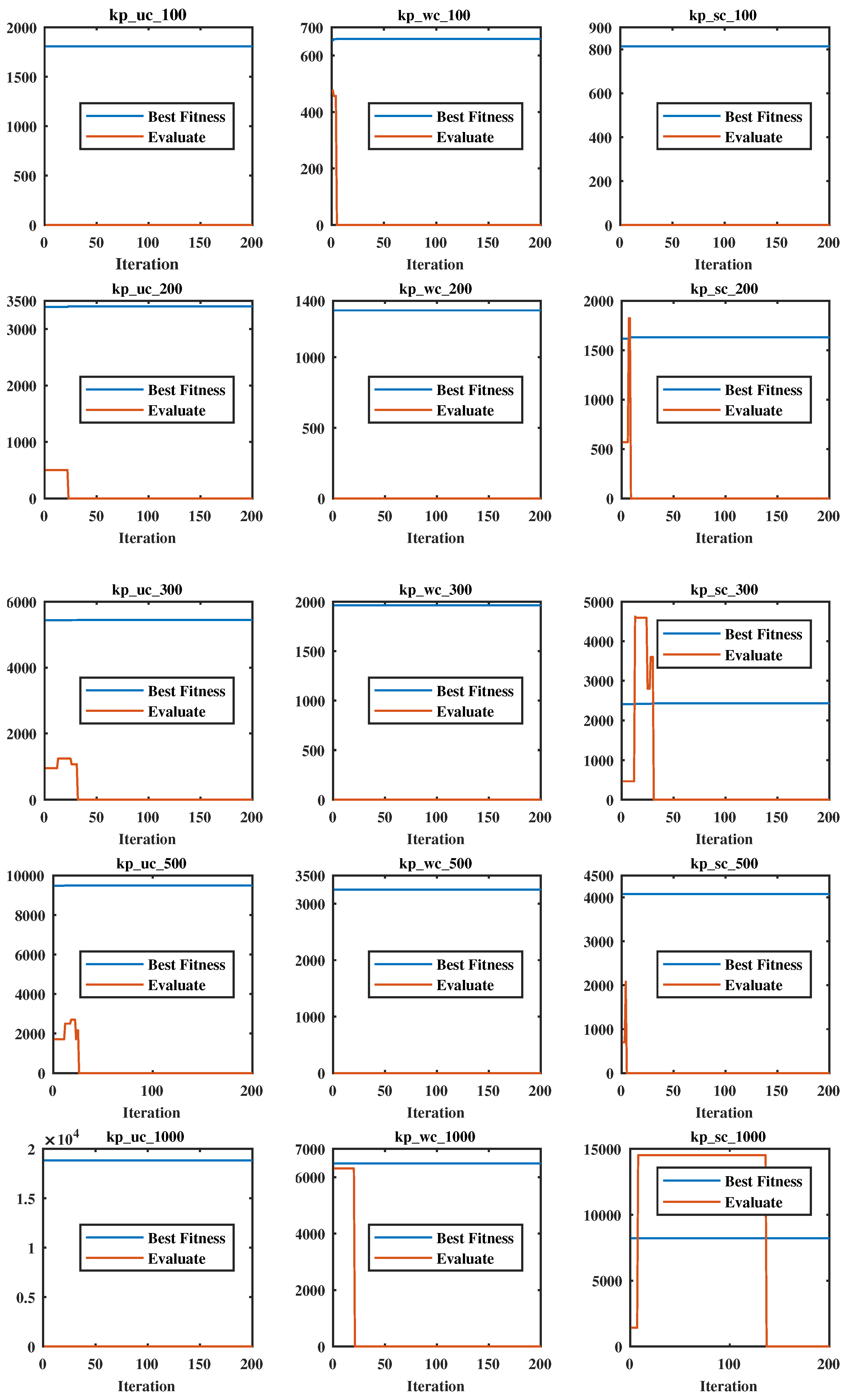
To evaluate the convergence performance of the algorithm, we introduce an evaluation metric, denoted as ${\mathrm{Evaluate}}^t$, which assesses the quality of the solutions by measuring the difference between the best solution and the optimal solution among the t-th generation individual. When items are ranked by their profit density in descending order, the difference between the best solution and the optimal solution often clusters around the break item b. Consequently, it is necessary to increase the weight of the serial number j corresponding to the position of the items. The calculation of $\mathrm{Evaluate}$ is as follows.

$$\begin{array}{c}\hfill {\mathrm{Evaluate}}^t=\sum _{j=1}^n\left(\right|y_{ij}^t-y_j^{*}|\times |b-j\left|\right)\mathrm{for}i=\underset{1\le k\le \mathrm{pop}}{argmax}f\left(Y_k^t\right)\end{array}$$

(19)

where $y_j^{*}$ is the j-th variable value of the optimal solution. Additionally, since the optimal solution to the problem is not necessarily unique, we set ${\mathrm{Evaluate}}^t=0$ if the objective function values of the best solution and the optimal solution coincide.

Based on the computational results of the IBPOA, the algorithm convergence and the evaluation curves are presented in Figure 3. The three columns correspond to kp_uc_n, kp_wc_n, and kp_sc_n, where $n=100,200,300,500,$ and 1000, respectively. The horizontal axis in all of the figures represents the iteration number. As shown in the figures, the objective function values obtained by the greedy algorithm demonstrate minimal deviation from the optimal solutions due to the inherent characteristics of the instances, resulting in relatively stable Best_Fitness values. However, the evaluation curves exhibit rapid convergence to zero with increasing iterations across most test cases. This pattern substantiates that the IBPOA can efficiently identify the optimal solutions for 0-1 knapsack problems, demonstrating both a robust global search capability and an effective local search performance.

4.4. An Analysis of the Population Diversity

In meta-heuristic algorithm iterations, the population diversity serves as a critical metric for evaluating the search capabilities, providing quantitative evidence of the ability to escape local optima. Typically, algorithms with strong population diversity exhibit high initial diversity levels that gradually decrease during optimization. To rigorously evaluate the performance of the IBPOA, we maintain a fixed population size of 30 and introduce the population diversity metric $\mathrm{pop}\_\mathrm{Div}$, defined as follows:

$$\begin{array}{c}\mathrm{pop}\_\mathrm{Div}=\sqrt{\sum _{i=1}^{\mathrm{pop}}\sum _{j=1}^n{(y_{ij}^t-{\overline{y}}_j^t)}^2}\end{array}$$

(20)

$$\begin{array}{c}{\overline{y}}_j^t={\displaystyle \frac{1}{\mathrm{pop}}}\sum _{i=1}^{\mathrm{pop}}{y}_{ij}\end{array}$$

(21)

The computational results are illustrated in Figure 4. As shown, the population diversity remains high during the initial iterations of the IBPOA. Notably, for the kp_wc_200 instance, where the greedy solution coincides with the global optimum, the population diversity metric remains zero throughout the optimization process. In kp_uc_n instances, due to significant disparities between the near-optimal solutions and the true optimum, the algorithm rapidly converges to the optimal solution. The local search operator subsequently exerts a minimal influence on individuals. Furthermore, under the moment of gravitation mechanism, individuals approaching the optimal solution are swiftly captured, leading to homogenization of the encodings and asymptotic convergence of the population diversity to zero. For the other instance categories, the population diversity progressively approaches zero with increasing iterations. Distinct from conventional meta-heuristic algorithms, the dual-operator framework of the IBPOA induces multi-modal diversity patterns contingent on the operator selection dynamics during the search process. These results align with theoretical expectations and validate the robust search capabilities of the algorithm.

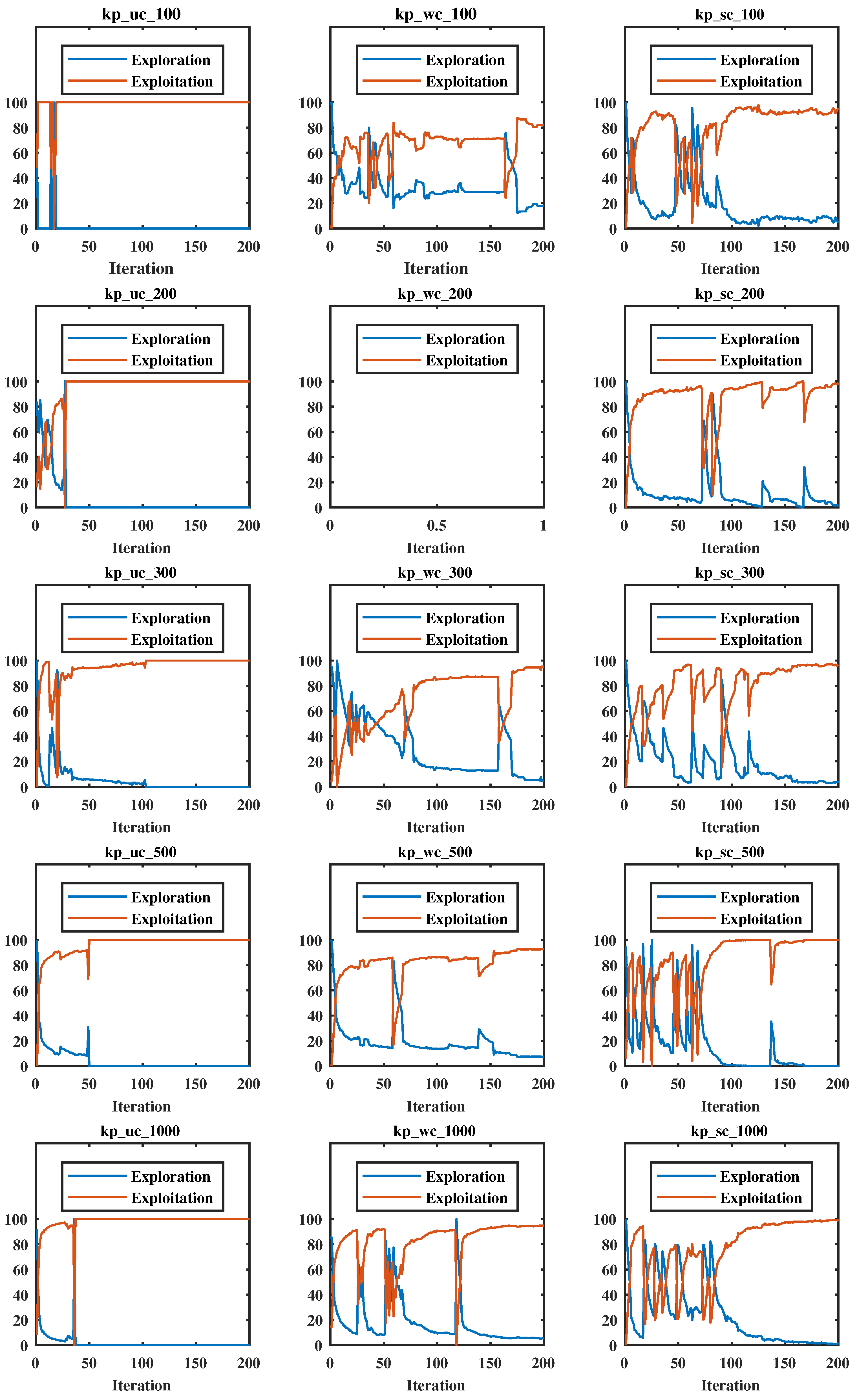
4.5. The Exploration and Exploitation Analysis

In addition to population diversity metrics, we introduce exploration and exploitation metrics to evaluate the algorithmic performance. Typically, algorithms demonstrating balanced exploration and exploitation capabilities exhibit behavioral trajectories where exploration dominates the initial phases, transitions through dynamic equilibrium in the intermediate stages, and culminates in the predominance of exploitation during the final iterations. Notably, algorithms employing multiple search operators may exhibit multi-modal patterns in these trajectories. The quantification methodology for exploration and exploitation is defined as follows:

$$\begin{array}{c}\mathrm{Exploration}(\%)={\displaystyle \frac{{\mathrm{Div}}^t}{{\mathrm{Div}}_{max}^t}}\times 100\end{array}$$

(22)

$$\begin{array}{c}\mathrm{Exploitation}(\%)={\displaystyle \frac{|{\mathrm{Div}}^t-{\mathrm{Div}}_{max}^t|}{{\mathrm{Div}}_{max}^t}}\times 100\end{array}$$

(23)

$$\begin{array}{c}{\mathrm{Div}}^t={\displaystyle \frac{1}{n}}\sum _{j=1}^n{\displaystyle \frac{1}{\mathrm{pop}}}\sum _{i=1}^{\mathrm{pop}}|{\overline{y}}_j^t-y_{ij}^t|\end{array}$$

(24)

The computational results are presented in Figure 5. Due to the inherent complexity of the instances, exploration and exploitation exhibit rapid dynamic interplay, followed by swift convergence during the initial iterations. Owing to the dual-operator framework, the algorithm maintains effective mechanisms for escaping from local optima, even as exploitation becomes predominant, as evidenced by the recurrent intersections between the exploration and exploitation curves. This behavior mitigates premature convergence and demonstrates robust adaptability.

4.6. An Ablation Study on the Transfer Functions

In Section 3.4, we analyzed the probability mapping spaces of both TFs by introducing the Lebesgue Measure. The theoretical results demonstrate that the ITF exhibits a smaller probability mapping space while ensuring the optimal solutions are preserved. To validate the superior performance of the ITF further, we not only provide theoretical guarantees but also conduct simulation experiments on 15 datasets (e.g., ‘kp_wc_n’). These empirical results confirm the efficacy of the improvements in the ITF.

To demonstrate the better performance of the ITF, we extend the POA framework by hybridizing the following transfer functions for algorithmic comparison. These include S-shaped [38], V-shaped [38], U-shaped [40], and taper-shaped [39] functions, proposed by Mirjalili and collaborators, along with the Z-shaped function introduced by Guo et al. [41]. Mathematical expressions of these TFs appear in Table 6, where column 1 lists the names of various transfer functions, columns 2 and 4 provide function symbols, and columns 3 and 5 present the corresponding mathematical expressions.

Table 6. Summary of compared transfer functions.

Name	Label	Expression	Label	Expression
S-shaped [38]	S1	${\mathrm{TF}}_1\left(x\right)={\displaystyle \frac{1}{1+e^{-2x}}}$	S3	${\mathrm{TF}}_3\left(x\right)={\displaystyle \frac{1}{1+e^{-x/2}}}$
	S2	${\mathrm{TF}}_2\left(x\right)={\displaystyle \frac{1}{1+e^{-x}}}$	S4	${\mathrm{TF}}_4\left(x\right)={\displaystyle \frac{1}{1+e^{-x/3}}}$
V-shaped [38]	V1	${\mathrm{TF}}_5\left(x\right)=\mathrm{erf}\left({\displaystyle \frac{\sqrt{\pi }}{2}}x\right)$	V3	${\mathrm{TF}}_7\left(x\right)={\displaystyle \frac{x}{\sqrt{1+x^2}}}$
	V2	${\mathrm{TF}}_6\left(x\right)=\left|tanh\left(x\right)\right|$	V4	${\mathrm{TF}}_8\left(x\right)=\left|{\displaystyle \frac{2}{\pi }}arctan\left({\displaystyle \frac{\pi }{2}}x\right)\right|$
U-shaped [40]	U1	${\mathrm{TF}}_9\left(x\right)={\left|x\right|}^{1.5}$	U3	${\mathrm{TF}}_{11}\left(x\right)={\left|x\right|}^3$
	U2	${\mathrm{TF}}_{10}\left(x\right)={\left|x\right|}^2$	U4	${\mathrm{TF}}_{12}\left(x\right)={\left|x\right|}^4$
Taper-shaped [39]	T1	${\mathrm{TF}}_{13}\left(x\right)={\displaystyle \frac{\sqrt{\left|x\right|}}{\sqrt{A}}}$	T2	${\mathrm{TF}}_{15}\left(x\right)={\displaystyle \frac{\sqrt[3]{\left|x\right|}}{\sqrt[3]{A}}}$
	T3	${\mathrm{TF}}_{14}\left(x\right)={\displaystyle \frac{\left|x\right|}{\left|A\right|}}$	T4	${\mathrm{TF}}_{16}\left(x\right)={\displaystyle \frac{\sqrt[4]{\left|x\right|}}{\sqrt[4]{A}}}$
Z-shaped [41]	Z1	${\mathrm{TF}}_{17}\left(x\right)=\sqrt{1-2^x}$	Z3	${\mathrm{TF}}_{19}\left(x\right)=\sqrt{1-8^x}$
	Z2	${\mathrm{TF}}_{18}\left(x\right)=\sqrt{1-5^x}$	Z4	${\mathrm{TF}}_{20}\left(x\right)=\sqrt{1-{20}^x}$

Table 6. Summary of compared transfer functions.

Name	Label	Expression	Label	Expression
S-shaped [38]	S1	${\mathrm{TF}}_1\left(x\right)={\displaystyle \frac{1}{1+e^{-2x}}}$	S3	${\mathrm{TF}}_3\left(x\right)={\displaystyle \frac{1}{1+e^{-x/2}}}$
	S2	${\mathrm{TF}}_2\left(x\right)={\displaystyle \frac{1}{1+e^{-x}}}$	S4	${\mathrm{TF}}_4\left(x\right)={\displaystyle \frac{1}{1+e^{-x/3}}}$
V-shaped [38]	V1	${\mathrm{TF}}_5\left(x\right)=\mathrm{erf}\left({\displaystyle \frac{\sqrt{\pi }}{2}}x\right)$	V3	${\mathrm{TF}}_7\left(x\right)={\displaystyle \frac{x}{\sqrt{1+x^2}}}$
	V2	${\mathrm{TF}}_6\left(x\right)=\left|tanh\left(x\right)\right|$	V4	${\mathrm{TF}}_8\left(x\right)=\left|{\displaystyle \frac{2}{\pi }}arctan\left({\displaystyle \frac{\pi }{2}}x\right)\right|$
U-shaped [40]	U1	${\mathrm{TF}}_9\left(x\right)={\left|x\right|}^{1.5}$	U3	${\mathrm{TF}}_{11}\left(x\right)={\left|x\right|}^3$
	U2	${\mathrm{TF}}_{10}\left(x\right)={\left|x\right|}^2$	U4	${\mathrm{TF}}_{12}\left(x\right)={\left|x\right|}^4$
Taper-shaped [39]	T1	${\mathrm{TF}}_{13}\left(x\right)={\displaystyle \frac{\sqrt{\left|x\right|}}{\sqrt{A}}}$	T2	${\mathrm{TF}}_{15}\left(x\right)={\displaystyle \frac{\sqrt[3]{\left|x\right|}}{\sqrt[3]{A}}}$
	T3	${\mathrm{TF}}_{14}\left(x\right)={\displaystyle \frac{\left|x\right|}{\left|A\right|}}$	T4	${\mathrm{TF}}_{16}\left(x\right)={\displaystyle \frac{\sqrt[4]{\left|x\right|}}{\sqrt[4]{A}}}$
Z-shaped [41]	Z1	${\mathrm{TF}}_{17}\left(x\right)=\sqrt{1-2^x}$	Z3	${\mathrm{TF}}_{19}\left(x\right)=\sqrt{1-8^x}$
	Z2	${\mathrm{TF}}_{18}\left(x\right)=\sqrt{1-5^x}$	Z4	${\mathrm{TF}}_{20}\left(x\right)=\sqrt{1-{20}^x}$

To standardize the discussion, we adopt a consistent naming convention for the POA hybridized with different TFs. For example, the POA integrated with transfer function S1 is denoted as BPOA-S1, with the other hybrid variants following the same naming scheme. Furthermore, to minimize the impact of the initial solutions, we fix the initial solution configuration as follows:

$$X^0={\left(\zeta \right)}_{\mathrm{pop}\times n}\mathrm{where}\zeta =-5.$$

During execution, if a solution $Y_i^t$ (corresponding to an individual encoding $X_i^t$ via TFs) violates the constraint $g\left(Y_i^t\right)\le C$, $Y_i^t$ is set to the zero vector ${\mathbf{0}}_n^{\top }$ and $X_i^t$ is reset to its initial state. The maximum iteration count is fixed at $\mathrm{MaxIter}=200$.

To validate the efficacy of the ITF, we conduct 30 independent runs comparing the BPOA-ITF against 20 BPOA variants hybridized with different TFs across three categories of instances. Detailed computational results are available at https://github.com/zhugemutian/Improved-Binary-Planet-Optimization-Algorithm, accessed on 14 May 2025.

Table 7 categorizes the performance outcomes relative to those of BPOA-ITF as superior, equivalent, inferior, or identical. Consistent with the prior methodology, these outcomes are symbolically represented as (+, −, ≈, =) to facilitate the comparative analysis. The statistical analysis reveals that the ITF demonstrates significant advantages $(p<0.05)$ over all 20 transfer functions across three categories of instances based on 30 independent runs.

Table 7. Summary of Wilcoxon’s rank-sum test results: BPOA-ITF versus BPOA-TFs.

BPOA-TFs v.s. BPOA-ITF	kp_uc_n				kp_wc_n				kp_sc_n
	+	≈	−	=	+	≈	−	=	+	≈	−	=
BPOA-S1	0	0	5	0	0	0	5	0	0	0	5	0
BPOA-S2	0	0	5	0	0	0	5	0	0	0	5	0
BPOA-S3	0	0	5	0	0	0	5	0	0	0	5	0
BPOA-S4	0	0	5	0	0	0	5	0	0	0	5	0
BPOA-V1	0	0	5	0	0	0	5	0	0	0	5	0
BPOA-V2	0	0	5	0	0	0	5	0	0	0	5	0
BPOA-V3	0	0	5	0	0	0	5	0	0	0	5	0
BPOA-V4	0	0	5	0	0	0	5	0	0	0	5	0
BPOA-U1	0	0	5	0	0	0	5	0	0	0	5	0
BPOA-U2	0	0	5	0	0	0	5	0	0	0	5	0
BPOA-U3	0	0	5	0	0	0	5	0	0	0	5	0
BPOA-U4	0	0	5	0	0	0	5	0	0	0	5	0
BPOA-T1	0	0	5	0	0	0	5	0	0	0	5	0
BPOA-T2	0	0	5	0	0	0	5	0	0	0	5	0
BPOA-T3	0	0	5	0	0	0	5	0	0	0	5	0
BPOA-T4	0	0	5	0	0	0	5	0	0	0	5	0
BPOA-Z1	0	0	5	0	0	0	5	0	0	0	5	0
BPOA-Z2	0	0	5	0	0	0	5	0	0	0	5	0
BPOA-Z3	0	0	5	0	0	0	5	0	0	0	5	0
BPOA-Z4	0	0	5	0	0	0	5	0	0	0	5	0

Table 7. Summary of Wilcoxon’s rank-sum test results: BPOA-ITF versus BPOA-TFs.

BPOA-TFs v.s. BPOA-ITF	kp_uc_n				kp_wc_n				kp_sc_n
	+	≈	−	=	+	≈	−	=	+	≈	−	=
BPOA-S1	0	0	5	0	0	0	5	0	0	0	5	0
BPOA-S2	0	0	5	0	0	0	5	0	0	0	5	0
BPOA-S3	0	0	5	0	0	0	5	0	0	0	5	0
BPOA-S4	0	0	5	0	0	0	5	0	0	0	5	0
BPOA-V1	0	0	5	0	0	0	5	0	0	0	5	0
BPOA-V2	0	0	5	0	0	0	5	0	0	0	5	0
BPOA-V3	0	0	5	0	0	0	5	0	0	0	5	0
BPOA-V4	0	0	5	0	0	0	5	0	0	0	5	0
BPOA-U1	0	0	5	0	0	0	5	0	0	0	5	0
BPOA-U2	0	0	5	0	0	0	5	0	0	0	5	0
BPOA-U3	0	0	5	0	0	0	5	0	0	0	5	0
BPOA-U4	0	0	5	0	0	0	5	0	0	0	5	0
BPOA-T1	0	0	5	0	0	0	5	0	0	0	5	0
BPOA-T2	0	0	5	0	0	0	5	0	0	0	5	0
BPOA-T3	0	0	5	0	0	0	5	0	0	0	5	0
BPOA-T4	0	0	5	0	0	0	5	0	0	0	5	0
BPOA-Z1	0	0	5	0	0	0	5	0	0	0	5	0
BPOA-Z2	0	0	5	0	0	0	5	0	0	0	5	0
BPOA-Z3	0	0	5	0	0	0	5	0	0	0	5	0
BPOA-Z4	0	0	5	0	0	0	5	0	0	0	5	0

5. Conclusions

The Planet Optimization Algorithm (POA), equipped with dual search operators, demonstrates a superior performance in escaping from the local optimal solution across 23 well-known test functions, 38 IEEE CEC benchmark test functions (CEC 2017, CEC 2019), and 3 real engineering problems in continuous optimization. Given the absence of binary POA variants, we propose the Improved Binary Planet Optimization Algorithm (IBPOA) by integrating the theoretical insights from branch-and-bound (B&B) and reduction algorithms with a hybrid greedy repair operator (GRO). The IBPOA leverages B&B theory to enhance the sigmoid transfer function. By ordering the items by profit density and establishing a symmetric hyperplane defined by the break item (denoted s) and the origin, it adjusts the selection probabilities symmetrically based on the items’ distances to this hyperplane, yielding the improved transfer function (ITF). Computational experiments on three categories of instances confirm that the IBPOA exhibits an exceptional performance in its convergence speed, population diversity, and exploration–exploitation balance.

Notably, the ITF demonstrates a superior performance on 15 benchmark instances compared to that of the other TFs. However, its reliance on linear relaxation and B&B theory introduces generalization limitations. When hybridized with algorithms solving other NP-hard problems, the ITF’s effectiveness varies due to problem-specific characteristics and linear relaxation methodologies. By leveraging linear relaxation and the theoretical results from B&B, a widely applicable transfer function for discrete optimization problems represents a promising research direction.

The future research directions are tripartite. Firstly, in terms of the algorithmic mechanisms, why the moment of gravitation outperforms direct gravitation in the operator selection should be investigated. Second, in terms of the theoretical bounds, we ought to determine whether empirically tuned parameters (e.g., $R_{min}$) possess theoretical upper bounds. Third, as regards the application scope, we could extend the IBPOA to combinatorial variants (e.g., set-union knapsack problems, discounted knapsack problems, and multi-dimensional knapsack problems).

References

1. Kellerer, H.; Pferschy, U.; Pisinger, D. Knapsack Problems; Springer: Berlin/Heidelberg, Germany, 2004. [Google Scholar]
2. Cook, S.A. The complexity of theorem-proving procedures. In Proceedings of the 3rd Annual ACM Symposium on Theory of Computing (STOC 1971), Shaker Heights, ON, USA, 3–5 May 1971; pp. 151–158. [Google Scholar]
3. Karp, R.M. Reducibility among Combinatorial Problems. In Complexity of Computer Computations; Miller, R.E., Thatcher, J.W., Bohlinger, J.D., Eds.; Springer: Boston, MA, USA, 1972; pp. 85–103. [Google Scholar]
4. Garey, M.R.; Johnson, D.S. Computer and Intractablility: A Guide to the Theory of NP-Completeness; Freeman: San Francisco, CA, USA, 1979. [Google Scholar]
5. Sulaiman, A.; Sadiq, M.; Mehmood, Y.; Akram, M.; Ali, G.A. Fitness-Based Acceleration Coefficients Binary Particle Swarm Optimization (FACBPSO) to Solve the Discounted Knapsack Problem. Symmetry 2022, 14, 1208. [Google Scholar] [CrossRef]
6. Beliakov, G. Knapsack problems with dependencies through non-additive measures and Choquet integral. Eur. J. Oper. Res. 2022, 301, 277–286. [Google Scholar] [CrossRef]
7. Tavana, M.; Keramatpour, M.; Santos-Arteaga, F.J.; Ghorbaniane, E. A fuzzy hybrid project portfolio selection method using Data Envelopment Analysis, TOPSIS and Integer Programming. Expert Syst. Appl. 2015, 42, 8432–8444. [Google Scholar] [CrossRef]
8. Sharafi, P.; Teh, L.H.; Hadi, M.N.S. Conceptual design optimization of rectilinear building frames: A Knapsack problem approach. Eng. Optimiz. 2014, 47, 1303–1323. [Google Scholar] [CrossRef]
9. Maher, S.J. A novel passenger recovery approach for the integrated airline recovery problem. Comput. Oper. Res. 2015, 57, 123–137. [Google Scholar] [CrossRef]
10. Wang, S.; Cui, W.; Chu, F.; Yu, J. The interval min–max regret knapsack packing-delivery problem. Int. J. Prod. Res. 2020, 59, 5661–5677. [Google Scholar] [CrossRef]
11. Bellman, R. Dynamic Programming; Princeton University Press: Princeton, NJ, USA, 1957. [Google Scholar]
12. Land, A.H.; Doig, A.G. An automatic method of solving discrete programming problem. Econometrica 1960, 28, 497–520. [Google Scholar] [CrossRef]
13. Toth, P. Dynamic programming algorithms for the Zero-One Knapsack Problem. Computing 1980, 25, 29–45. [Google Scholar] [CrossRef]
14. Holland, J.H. Adaptation in Natural and Artificial Systems; MIT Press: Cambridge, MA, USA, 1975. [Google Scholar]
15. Mirjalili, S.; Mirjalili, S.M.; Lewis, A. Grey wolf optimizer. Adv. Eng. Softw. 2014, 69, 46–61. [Google Scholar] [CrossRef]
16. Tanweer, M.R.; Suresh, S.; Sundararajan, N. Dynamic mentoring and self-regulation based particle swarm optimization algorithm for solving complex real-world optimization problems. Inf. Sci. 2016, 326, 1–24. [Google Scholar] [CrossRef]
17. Nikolić, M.; Teodorović, D. Transit network design by bee colony optimization. Expert Syst. Appl. 2013, 40, 5945–5955. [Google Scholar] [CrossRef]
18. Thanh, S.-T.; Minh, H.-L.; Magd, A.W.; Thanh, C.-L. An efficient Planet Optimization Algorithm for solving engineering problems. Sci. Rep. 2022, 12, 8362. [Google Scholar] [CrossRef] [PubMed]
19. Yang, Y. An upper bound of the mutation probability in the genetic algorithm for general 0-1 knapsack problem. arXiv 2024, arXiv:2403.11307. [Google Scholar]
20. Ervural, B.; Hakli, H. A binary reptile search algorithm based on transfer functions with a new stochastic repair method for 0-1 knapsack problems. Comput. Ind. Eng. 2023, 178, 109080. [Google Scholar] [CrossRef]
21. Zhou, Y.Q.; Shi, Y.; Wei, Y.F.; Luo, Q.F.; Tang, Z.H. Nature-inspired algorithms for 0-1 knapsack problem: A survey. Neurocomputing 2023, 554, 126630. [Google Scholar] [CrossRef]
22. Shu, Z.; Ye, Z.W.; Zong, X.L.; Liu, S.Q.; Zhang, D.D.; Wang, C.Z.; Wang, M.W. A modified hybrid rice optimization algorithm for solving 0-1 knapsack problem. Appl. Intell. 2022, 52, 5751–5769. [Google Scholar] [CrossRef]
23. Yildizdan, G.; Baş, E. A Novel Binary Artificial Jellyfish Search Algorithm for Solving 0-1 Knapsack Problems. Neural Process Lett. 2023, 55, 8605–8671. [Google Scholar] [CrossRef]
24. Abdel-Basset, M.; Mohamed, R.; Chakrabortty, R.K.; Ryan, M.; Mirjalili, S. New binary marine predators optimization algorithms for 0-1 knapsack problems. Comput. Ind. Eng. 2021, 151, 106949. [Google Scholar] [CrossRef]
25. Lim, T.Y.; Al-Betar, M.A.; Khader, A.T. Taming the 0/1 knapsack problem with monogamous pairs genetic algorithm. Expert Syst. Appl. 2016, 54, 241–250. [Google Scholar] [CrossRef]
26. Zhou, Y.Q.; Li, L.L.; Ma, M.Z. A Complex-valued Encoding Bat Algorithm for Solving 0-1 Knapsack Problem. Neural Process Lett. 2016, 44, 407–430. [Google Scholar] [CrossRef]
27. Zhou, Y.Q.; Bao, Z.F.; Luo, Q.F.; Zhang, S. A complex-valued encoding wind driven optimization for the 0-1 knapsack problem. Appl. Intell. 2017, 46, 684–702. [Google Scholar] [CrossRef]
28. Pavithr, R.S.; Gursaran. Quantum Inspired Social Evolution (QSE) algorithm for 0-1 knapsack problem. Swarm Evol. Comput. 2016, 29, 33–46. [Google Scholar] [CrossRef]
29. Wang, Y.; Wang, W. Quantum-Inspired Differential Evolution with Grey Wolf Optimizer for 0-1 Knapsack Problem. Mathematics 2021, 9, 1233. [Google Scholar] [CrossRef]
30. Bhattacharjee, K.K.; Sarmah, S.P. Shuffled frog leaping algorithm and its application to 01 knapsack problem. Appl. Soft Comput. 2014, 19, 252–263. [Google Scholar] [CrossRef]
31. Kennedy, J.; Eberhart, R.C. Particle swarm optimization. In Proceedings of the 1995 IEEE International Conference on Neural Networks (ICNN), Perth, WA, Australia, 27 November–1 December 1995; pp. 1942–1948. [Google Scholar]
32. Kennedy, J.; Eberhart, R.C. Discrete binary version of the particle swarm algorithm. In Proceedings of the IEEE International Conference on Systems, Man and Cybernetics, Orlando, FL, USA, 12–15 October 1997; Volume 5, pp. 4104–4108. [Google Scholar]
33. Rajwar, K.; Deep, K.; Das, S. An exhaustive review of the metaheuristic algorithms for search and optimization: Taxonomy, applications, and open challenges. Artif. Intell. Rev. 2023, 56, 13187–13257. [Google Scholar] [CrossRef] [PubMed]
34. Molina, D.; Poyatos, J.; Del Ser, J.; García, S.; Hussain, A.; Herrera, F. Comprehensive taxonomies of nature-and bio-inspired optimization: Inspiration versus algorithmic behavior, critical analysis recommendations. Cogn. Comput. 2020, 12, 897–939. [Google Scholar] [CrossRef]
35. Mirjalili, S. SCA: A sine cosine algorithm for solving optimization problems. Knowl.-Based Syst. 2016, 96, 120–133. [Google Scholar] [CrossRef]
36. Suid, M.H.; Ahmad, M.A.; Nasir, A.N.K.; Ghazali, M.R.; Jui, J.J. Continuous-time Hammerstein model identification utilizing hybridization of Augmented Sine Cosine Algorithm and Game-Theoretic approach. Results Eng. 2024, 23, 102506. [Google Scholar] [CrossRef]
37. Mirjalili, S. Moth-flame optimization algorithm: A novel nature-inspired heuristic paradigm. Knowl.-Based Syst. 2015, 89, 228–249. [Google Scholar] [CrossRef]
38. Mirjalili, S.; Lewis, A. S-shaped versus V-shaped transfer functions for binary Particle Swarm Optimization. Swarm Evol. Comput. 2013, 9, 1–14. [Google Scholar] [CrossRef]
39. He, Y.; Zhang, F.; Mirjalili, S.; Zhang, T. Novel binary differential evolution algorithm based on Taper-shaped transfer functions for binary optimization problems. Swarm Evol. Comput. 2022, 69, 101022. [Google Scholar] [CrossRef]
40. Mirjalili, S.; Zhang, H.; Mirjalili, S.; Chalup, S.; Noman, N. A Novel U-shaped transfer function for binary particle swarm optimisation. Adv. Intell. Syst. Comput. 2020, 1138, 241–259. [Google Scholar]
41. Guo, S.S.; Wang, J.S.; Guo, M.W. Z-Shaped Transfer Functions for Binary Particle Swarm Optimization Algorithm. Comput. Intell. Neurosci. 2020, 2020, 6502807. [Google Scholar] [CrossRef] [PubMed]
42. Clerc, M. Particle Swarm Optimization; ISTE: Washington, DC, USA, 2006. [Google Scholar]
43. Wang, W.B. Research on Particle Swarm Optimization Algorithm and Its Application. Ph.D. Thesis, Southwest Jiaotong University, Chengdu, China, 2012. [Google Scholar]
44. Wang, D.S.; Tan, D.P.; Liu, L. Particle swarm optimization algorithm: An overview. Soft Comput. 2018, 22, 387–408. [Google Scholar] [CrossRef]
45. Kennedy, J.; Mendes, R. Neighborhood topologies in fully informed and best-of-neighborhood particle swarms. IEEE Trans. Syst. Man Cybern. Part C 2006, 36, 515–519. [Google Scholar] [CrossRef]
46. Ye, W.; Feng, W.; Fan, S. A novel multi-swarm particle swarm optimization with dynamic learning strategy. Appl. Soft Comput. 2017, 61, 832–843. [Google Scholar] [CrossRef]
47. Dey, S.S.; Dubey, Y.; Molinaro, M. Branch-and-bound solves random binary IPs in poly(n)-time. Math. Program. 2023, 200, 569–587. [Google Scholar] [CrossRef]
48. Dantzig, G.B. Discrete-Variable Extremum Problems. Oper. Res. 1957, 5, 266–288. [Google Scholar] [CrossRef]
49. Mezura-Montes, E.; Coello Coello, C.A. Constraint-handling in nature-inspired numerical optimization: Past, present and future. Swarm Evol. Comput. 2011, 1, 173–194. [Google Scholar] [CrossRef]
50. Samanipour, F.; Jelovica, J. Adaptive repair method for constraint handling in multi-objective genetic algorithm based on relationship between constraints and variables. Appl. Soft Comput. 2020, 90, 106143. [Google Scholar] [CrossRef]
51. Bansal, J.C.; Deep, K. A modified binary particle swarm optimization for knapsack problems. Appl. Math. Comput. 2012, 218, 11042–11061. [Google Scholar] [CrossRef]
52. Chen, Y.; Xie, W.C.; Zou, X.F. A binary differential evolution algorithm learning from explored solutions. Neurocomputing 2015, 149, 1038–1047. [Google Scholar] [CrossRef]
53. Hota, A.R.; Pat, A. An adaptive quantum-inspired differential evolution algorithm for 0-1 knapsack problem. In Proceedings of the IEEE 2nd World Congress on Nature and Biologically Inspired Computing (NaBIC 10), Kitakyushu, Japan, 15–17 December 2010; pp. 703–708. [Google Scholar]
54. Peng, H.; Wu, Z.J.; Shao, P.; Deng, C.S. Dichotomous binary differential evolution for Knapsack problems. Math. Probl. Eng. 2016, 2016, 5732489. [Google Scholar] [CrossRef]
55. Ali, I.M.; Essam, D.; Kasmarik, K. Novel binary differential evolution algorithm for knapsack problems. Inf. Sci. 2021, 542, 177–194. [Google Scholar] [CrossRef]
56. Löfberg, J. YALMIP: A Toolbox for Modeling and Optimization in MATLAB. In Proceedings of the CACSD Conference, Taipei, China, 2–4 September 2004. [Google Scholar]
Figure 1. A comparison of two decoding methods.
Symmetry 17 01538 g001
Figure 2. A flowchart of a basic genetic algorithm.
Symmetry 17 01538 g002
Figure 3. The convergence curve and the Evaluate curve.
Symmetry 17 01538 g003
Figure 4. The population diversity.
Symmetry 17 01538 g004
Figure 5. The exploration and exploitation of the IBPOA.
Symmetry 17 01538 g005
Disclaimer/Publisher’s Note: The statements, opinions and data contained in all publications are solely those of the individual author(s) and contributor(s) and not of MDPI and/or the editor(s). MDPI and/or the editor(s) disclaim responsibility for any injury to people or property resulting from any ideas, methods, instructions or products referred to in the content.