Sailfish Optimization Algorithm Integrated with the Osprey Optimization Algorithm and Cauchy Mutation and Its Engineering Applications

Abstract

From collective intelligence to evolutionary computation and machine learning, symmetry can be leveraged to enhance algorithm performance, streamline computational procedures, and elevate solution quality. Grasping and leveraging symmetry can give rise to more resilient, scalable, and understandable algorithms. In view of the flaws of the original Sailfish Optimization Algorithm (SFO), such as low convergence precision and a propensity to get stuck in local optima, this paper puts forward an Osprey and Cauchy Mutation Integrated Sailfish Optimization Algorithm (OCSFO). The enhancements are mainly carried out in three aspects: (1) Using the Logistic map to initialize the sailfish and sardine populations. (2) In the first stage of the local development phase of sailfish individual position update, adopting the global exploration strategy of the Osprey Optimization Algorithm to boost the algorithm’s global search capability. (3) Introducing Cauchy mutation to activate the sailfish and sardine populations during the prey capture stage. Through the comparative analysis of OCSFO and seven other swarm intelligence optimization algorithms in the optimization of 23 classic benchmark test functions, as well as the Wilcoxon rank-sum test, it is evident that the optimization speed and convergence precision of OCSFO have been notably improved. To confirm the practicality and viability of the OCSFO algorithm, it is applied to solve the optimization problems of piston rods, three-bar trusses, cantilever beams, and topology. Through experimental analysis, it can be concluded that the OCSFO algorithm has certain advantages in solving practical optimization problems.

1. Introduction

With the ongoing progress and evolution of society, the attributes of engineering optimization problems have undergone significant transformations. These issues have developed from small-scale and simple structures to large-scale and highly intricate systems, from single-peak solution landscapes to multi-peak setups, and from linear to strongly non-linear features [1,2]. Such changes present considerable challenges to traditional optimization algorithms, which usually depend on accurate mathematical models and gradient-based techniques. When dealing with large-scale, multi-peak, and non-linear problems, these conventional algorithms struggle to efficiently explore the solution space [3]. As a result, they often fail to find the global optimal solution or get stuck in local optima, making them insufficient for dealing with the increasing complexity of modern engineering optimization tasks [4,5]. In the complex realm of computational algorithms, symmetry appears as a powerful yet underappreciated concept with broad implications. For instance, in swarm intelligence, the behavioral patterns of social insects like ants and bees inherently show symmetrical properties. Ant colonies display symmetrical foraging patterns around their nests when searching for food. By imitating this symmetry in artificial swarm intelligence algorithms, such as Ant Colony Optimization (ACO), more effective search strategies can be created. ACO algorithms make use of the symmetrical distribution of pheromone trails left by ants to guide the search process, ensuring a balanced exploration of all potential paths. This symmetry-driven method not only speeds up the convergence towards optimal solutions but also lowers the chance of being trapped in local optima.

Evolutionary computation, inspired by biological evolution, also gains a lot from symmetry. Genetic algorithms, a typical case, work based on genetic operators such as crossover and mutation. By incorporating symmetry into the encoding of genetic information, more efficient and effective search spaces can be built. For example, symmetrical chromosome representations can ensure that similar genetic configurations are grouped together, facilitating a more systematic exploration of the solution space. This allows for faster evolution of superior solutions, as the algorithm can more easily recognize and spread beneficial genetic traits. Swarm intelligence optimization algorithms have become a promising alternative. Based on the study of group behavior in nature, these algorithms take inspiration from the collective activities of biological groups like ants, birds, and fish [6]. They imitate behaviors such as ant foraging, bird flocking, or fish schooling. By emulating these natural behaviors, swarm intelligence algorithms use information exchange and cooperation mechanisms among group members [7,8], enabling a more comprehensive exploration of the solution space and a gradual convergence towards the optimal solution for a specific problem. Their unique ability to handle complex and uncertain situations has led to their wide application in solving various complex optimization problems [9]. For example, in path planning for autonomous vehicles or drones, these algorithms can efficiently find the shortest and safest routes while avoiding obstacles. In workshop scheduling, they can optimize resource allocation (such as machines and labor) to minimize production time and costs [10]. These applications show the effectiveness and versatility of swarm intelligence optimization algorithms in addressing real-world complex optimization challenges.

The Sailfish Optimization Algorithm (SFO), put forward by scholar Shadravan in 2019, is a notable addition to the family of swarm intelligence optimization algorithms [11]. This algorithm is cleverly designed based on the hunting dynamics between sailfish (predators) and sardines (prey) in marine ecosystems. In the SFO framework, sailfish are regarded as candidate solutions for the optimization problem, with their positions in the solution space corresponding to potential solutions that are updated iteratively to approach the optimal solution. Sardines, on the other hand, play a crucial role in enhancing the algorithm’s randomness by introducing unpredictability, which helps the algorithm avoid local optima and promotes a more thorough exploration of the solution space [12]. During the optimization process, the SFO algorithm simulates three different behavioral strategies that occur when sailfish groups hunt sardine schools. The first is the population elite strategy, in which the best-performing sailfish (elite solutions) guide the movement of other members of the population. By sharing their information and positions, elite sailfish help the entire group converge more quickly towards promising areas of the solution space. The second is the alternating attack strategy [13], which imitates the way sailfish take turns attacking sardine schools from different directions. Through alternating attack patterns, the algorithm can explore various parts of the solution space, increasing the probability of finding the global optimal solution. The third is the prey capture strategy, which focuses on the actual process of sailfish catching sardines. In an algorithmic context, this represents the exploitation phase, where the algorithm refines identified solutions and seeks a more precise convergence towards the optimal solution. Through these three strategies, the SFO algorithm systematically searches for feasible solutions within the solution space, gradually getting closer to the optimal solution.

The SFO algorithm has been widely applied and studied in many fields. In engineering design, it has been used to optimize the parameters of mechanical systems, electrical circuits, and structural designs, enabling performance improvements while reducing costs. In data mining and machine learning, it has been used for tasks such as feature selection, classifier parameter tuning, and clustering, improving the efficiency and accuracy of these algorithms. These applications have, to a certain extent, verified the flexibility and reliability of the SFO algorithm, showing its potential to become a powerful tool in the optimization field.

The following are this paper’s primary contributions:

• Propose an OCSFO hybrid algorithm that enhances global exploration capability through OOA and avoids local optima by combining Cauchy mutation;
• Design a multi-stage adaptive parameter strategy to dynamically balance search accuracy and speed;
• Validate algorithm performance in 23 benchmark functions and 4 types of engineering problems, outperforming 7 compared algorithms.

2. Related Work

Analogous to other swarm intelligence optimization algorithms, the SFO algorithm also faces drawbacks, including a tendency to converge to local optima and a sluggish convergence rate. To boost SFO’s optimization capacity and expedite its convergence, many scholars have put forward various enhancements. Reference [14] presented a new DESFO algorithm that combines the Differential Evolution (DE) algorithm with SFO. When utilized for feature selection tasks, this algorithm can effectively pinpoint the most discriminative features and showcases remarkable advantages in both convergence speed and accuracy. Reference [15] proposed an improved ISFO algorithm by integrating an adaptive non-linear iteration factor, Lévy flight strategy, and differential mutation strategy. Experimental results indicate that the ISFO algorithm displays superior robustness and precision on standard test functions. Reference [16] enhanced the SFO algorithm through strategies such as inertia weight adjustment, modification of the global search formula, and adoption of the Lévy flight strategy. This improved variant was successfully applied to select optimal controller nodes from a group of sensor nodes, yielding favorable results. Reference [17] developed an advanced SFO algorithm with enhanced performance by introducing two search strategies: population switching and random mutation. When tested on the CEC2017 benchmark suite and classical engineering problems, this improved algorithm demonstrated notably higher convergence accuracy.

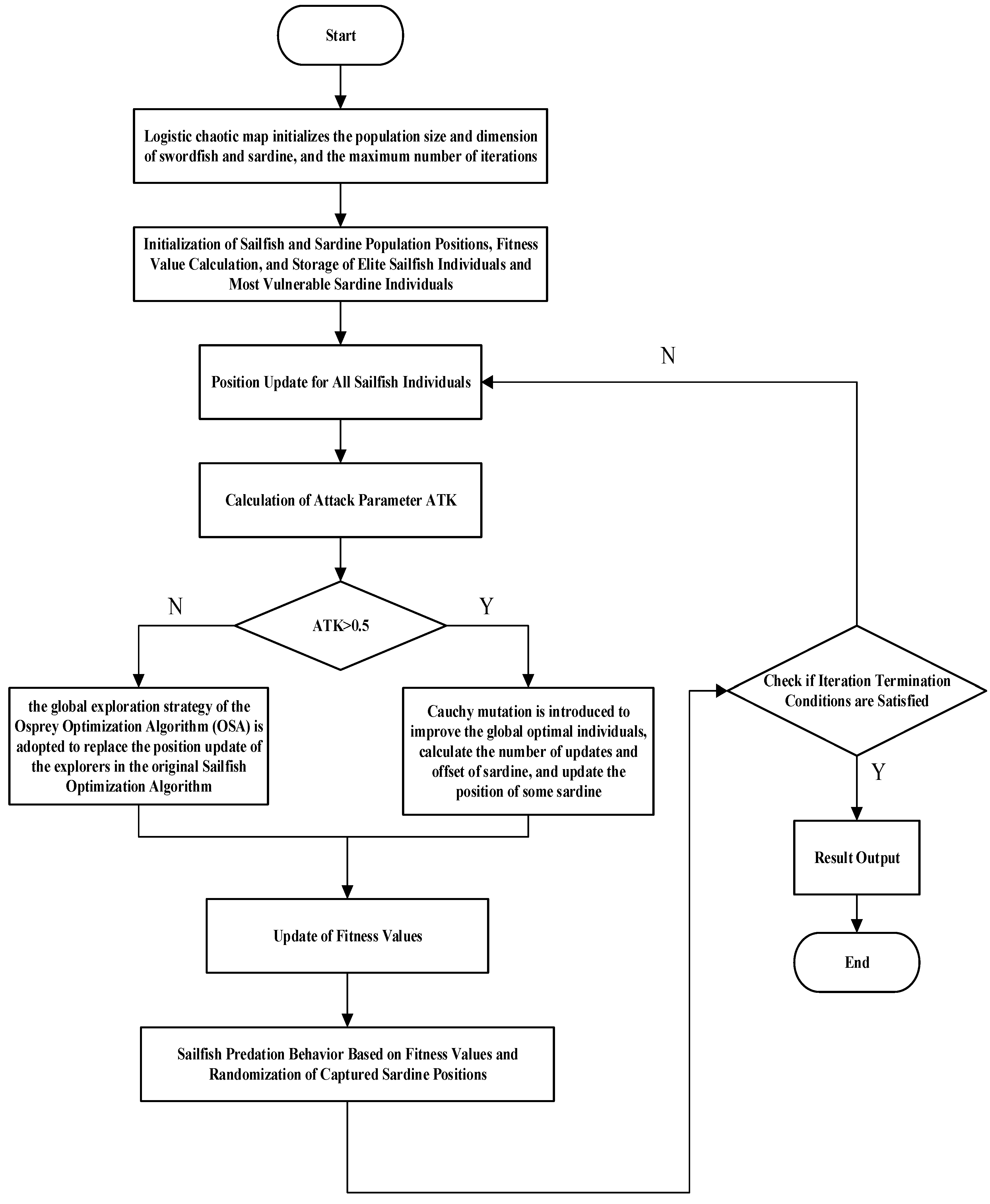
While the above-mentioned improved algorithms have enhanced the optimization performance of the standard SFO to varying degrees, they still encounter challenges such as premature convergence and vulnerability to local optima when tackling complex multi-peak problems. To further enhance SFO’s performance, this paper proposes an Osprey and Cauchy Mutation Integrated Sailfish Optimization Algorithm (OCSFO). The improvements are carried out in three key aspects:

(1) Initializing the sailfish and sardine populations using the Logistic map to enhance population diversity;

(2) Employing the global exploration strategy of the Osprey Optimization Algorithm during the first stage of the local development phase in sailfish individual position updates, thereby strengthening the algorithm’s global search capability;

(3) Introducing Cauchy mutation to stimulate the activity of sailfish and sardine populations during the prey capture stage, enhancing local exploitation and escaping from local optima.

Subsequently, OCSFO is tested on 23 classical benchmark test functions, and four engineering design optimization problems to verify its effectiveness in solving complex optimization tasks.

3. Standard Sailfish Optimization Algorithm

The conventional Sailfish Optimization Algorithm (SFOA) comprises two populations. One is the sailfish population, which conducts searches around the current optimal solution’s location to enhance the local search capability [18,19]. The other is the sardine population. As the prey of sailfish, the sardine population explores positions within the search space to improve the global search comprehensiveness. Sailfish are capable of searching in multi-dimensional spaces [20]. Thus, sailfish are regarded as candidate solutions, and the number of variables in the problem to be solved corresponds to the dimension of the search space, which is represented as the sailfish’s position in the algorithm. The standard Sailfish Optimization Algorithm includes four steps [21]:

(1) Population Initialization

As a population-based meta-heuristic algorithm, in the Sailfish Optimization Algorithm, it is assumed that sailfish stand for candidate solutions, and the problem variables are equivalent to the sailfish’s positions in the search space. Correspondingly, the population in the solution space is generated randomly. Sailfish can perform searches in one-dimensional, two-dimensional, three-dimensional, or even higher-dimensional spaces, and their position vectors are changeable [22]. In a d-dimensional search space, the current position of $S{F}_{\mathrm{i}k}\in R(i=1,2,\dots ,m)$ of the i-th member in the k-th search is

$$S{F}_{position}=\left[\begin{array}{cccc}S{F}_{1,1}& S{F}_{1,2}& \dots & S{F}_{1,d}\\ S{F}_{2,1}& S{F}_{2,2}& \dots & S{F}_{2,d}\\ ⋮& ⋮& ⋮& ⋮\\ S{F}_{m,1}& S{F}_{m,2}& \dots & S{F}_{m,d}\end{array}\right]$$

(1)

where, the parameter m represents the number of sailfish, d represents the number of variables, and SF_ij represents the value of the i-th sailfish in the j-th dimension. In addition, the fitness of each sailfish is calculated through the fitness function as follows:

$$\mathit{fitness} \mathit{value} \mathit{of} \mathit{sailfish}=f(\mathit{sailfish})=f(S{F}_1,S{F}_2,\dots ,S{F}_m)$$

(2)

To evaluate each sailfish, the following matrix shows the fitness values of all solutions:

$$S{F}_{Fitness}=\left[\begin{array}{c}f\left(\begin{array}{cccc}S{F}_{1,1}& S{F}_{1,2}& \dots & S{F}_{1,d}\end{array}\right)\\ f\left(\begin{array}{cccc}S{F}_{2,1}& S{F}_{2,2}& \dots & S{F}_{2,d}\end{array}\right)\\ ⋮\\ f\left(\begin{array}{cccc}S{F}_{m,1}& S{F}_{m,2}& \dots & S{F}_{m,d}\end{array}\right)\end{array}\right]=\left[\begin{array}{c}{F}_{S{F}_1}\\ F_{S{F}_2}\\ ⋮\\ F_{S{F}_m}\end{array}\right]$$

(3)

where, the parameter m is the number of sailfish, SF_ij is the value of the i-th sailfish in the j-th dimension, the parameter f is the fitness function used for calculation, and SF_Fitness is used to store the fitness values returned for each sailfish’s fitness or objective function value [23]. The first row of the matrix SF_position is fed into the fitness function, and its output represents the fitness value of the corresponding sailfish in the SF_Fitness matrix.

The sardine population is another important component of the Sailfish Optimization Algorithm. The algorithm assumes that the sardine school also swims in the search space. Therefore, the positions of the sardines and their fitness values are utilized as follows:

$$S{F}_{position}=\left[\begin{array}{cccc}S{F}_{1,1}& S{F}_{1,2}& \dots & S{F}_{1,d}\\ S{F}_{2,1}& S{F}_{2,2}& \dots & S{F}_{2,d}\\ ⋮& ⋮& ⋮& ⋮\\ S{F}_{n,1}& S{F}_{n,2}& \dots & S{F}_{n,d}\end{array}\right]$$

(4)

The parameter n is the number of sardines, S_ij is the value of the i-th sardine in the j-th dimension, and the S_position matrix represents the positions of all sardines [24].

$$S_{Fitness}=\left[\begin{array}{c}f\left(\begin{array}{cccc}{S}_{1,1}& S_{1,2}& \dots & S_{1,d}\end{array}\right)\\ f\left(\begin{array}{cccc}{S}_{2,1}& S_{2,2}& \dots & S_{2,d}\end{array}\right)\\ ⋮\\ f\left(\begin{array}{cccc}{S}_{m,1}& S_{m,2}& \dots & S_{m,d}\end{array}\right)\end{array}\right]=\left[\begin{array}{c}{F}_{S_1}\\ F_{S_2}\\ ⋮\\ F_{S_m}\end{array}\right]$$

(5)

The parameter n is the number of sardines, S_ij represents the value of the i-th sardine in the j-th dimension, f is the objective function, and it is used to store the fitness value of each sardine. It is worth noting that the sailfish and sardines are corresponding factors in finding solutions. In this algorithm, the sailfish are the main factor, scattered in the search space, while the sardines can cooperate to find the best position in the area. In fact, when searching the space, the sardines may be preyed upon by the sailfish. If a sailfish discovers a better solution obtained so far, it will update its position [25].

(2) Population Elite Strategy

To enable the algorithm to retain the optimal solution of each iteration, the population elite strategy is introduced. The individual with the highest fitness value in the sailfish population is selected as the elite sailfish for each attack iteration $X_{elite\_SF}^i$. The individual with the highest fitness value in the sardine population is selected as the injured sardine $X_{injured\_S}^i$ that is most likely to be captured after being attacked by the sailfish in each iteration [26].

(3) Alternating Attack Strategy

During the process of preying on sardines, sailfish adopt an alternating attack method, which can minimize the energy consumption of sailfish and make it easier to capture sardines. The SFO algorithm simulates this process, and the position update formula of the sailfish is as follows:

$$X_{new\_SF}^i=X_{elite\_SF}^i-{\lambda }_i\times \left(rand(0,1)\times \left({\displaystyle \frac{X_{elite\_SF}^i+X_{injured\_S}^i}{2}}\right)-X_{\mathrm{old}\_\mathrm{SF}}^i\right)$$

(6)

Wherein,$X_{elite\_SF}^i$ is the position of the elite sailfish formed up to the current time, $X_{injured\_S}^i$ determines the best position of the injured sardine formed currently, $X_{\mathrm{old}\_\mathrm{SF}}^i$ is the current position of the sailfish, rand (0,1) is a random number between 0 and 1, and i is a coefficient generated in the i-th iteration. The generation method is as follows [27]:

$${\lambda }_i=2\times rand\times PD-PD$$

(7)

where PD is a factor set considering the change in prey density caused by the predation of sailfish during the hunting period. The generation formula is as follows:

$$PD=1-{\displaystyle \frac{N_{SF}}{N_{SF}+N_S}}$$

(8)

N_SF and N_S are the number of sailfish and sardines in the loop, respectively.

(4) Prey Capture Strategy

In the SFO algorithm, the random update of the sardine population’s position helps to find the optimal solution in the search space, thereby simulating the process of sailfish capturing sardines. The sardines update their positions in each iteration based on the current attack power of the sailfish and the current best position. The position update formula is as follows [28]:

$$X_{newS}^i=r\times (X_{eliteSF}^i-X_{oldS}^i+AP)$$

(9)

The position of the sardine before update is $X_{oldS}^i$, the position after update is $X_{newS}^i$, the parameter r is a random number between 0 and 1, The parameter AP is the attack power of the sailfish in each iteration, and its value gradually decreases as the number of iterations increases. The generation formula is as follows:

$$AP=A\times (1-(2\times t\times \epsilon ))$$

(10)

The parameters A and $\epsilon$ are coefficients that make the attack power AP decrease from A to 0. The AP parameter helps to balance the exploration and exploitation of the search space. When the attack power of the sailfish is high (i.e., AP ≥ 0.5, all sardine positions are updated. When the attack power of the sailfish is low (i.e., AP < 0.5), only the positions of α sardines with a shift amount of β are updated. The calculation formulas for α and β are as follows:

$$\alpha =N_s\times AP$$

(11)

$$\beta =d_i\times AP$$

(12)

The parameter d_i is the dimension of the sardine, and N_s is the number of sardines.

When the fitness value of the updated sardine is better than that of the sailfish, the process of the sailfish capturing the sardine is simulated. The position of the sailfish at the current position is replaced with the position of the current sardine, and the position of the replaced sardine is randomized. The formula is as follows:

$$X_{SF}^i=X_S^i if f(S_i)<f(S{F}_i)$$

(13)

The parameter $X_{SF}^i$ is the position of the sailfish in the i-th iteration. The parameter $X_S^i$ is the position of sardine in the i-th iteration.

Summarizing the above operating mechanism of the Sailfish Optimization Algorithm, the steps of the SFO algorithm can be simplified as follows:

Step 1: Parameter Setting. Set the sailfish population size M, the sardine population size N, the search space dimension D, the maximum number of iterations Maxiter, and the non-linear factor parameters A = 4 and ε = 0.01 in the algorithm.

Step 2: Population Initialization. Initialize the positions of the sailfish and sardine populations in the search space.

Step 3: Elite Selection. Calculate the fitness values of each sailfish and sardine, record and find the positions and fitness values of the optimal individuals among them. Select the sailfish with the best fitness value $X_{elite\_SF}^i$ as the elite sailfish, and select the sardine with the best fitness value $X_{injured\_S}^i$ as the injured sardine.

Step 4: Start Iteration. Update the positions of the sailfish according to Formula (6) and the positions of the sardines according to Formula (9). Consider the attack power factor. If the attack power AP < 0.5, calculate α and β according to Formulas (11) and (12), and update the positions of some sardines. Otherwise, update the positions of all sardines.

Step 5: Fitness Value. Evaluation of Sailfish and Sardines Determine whether to perform position replacement.

Step 6: Calculate the Fitness Values of Sailfish and Sardines Record and update the global optimal value and position.

Step 7: Check Iteration Termination Condition. If the current iteration meets the termination condition, stop the iteration and output the global optimal solution. Otherwise, jump to Step 3 to continue the iterative operation.

4. Osprey and Cauchy Mutation Integrated Sailfish Optimization Algorithm

4.1. Chaotic Map Initialization

The population initialization method has a certain impact on the optimization effect and robustness of swarm intelligence algorithms [29]. Compared with completely random population initialization, introducing an appropriate chaotic sequence for initialization can generate a more uniformly distributed initial population in the search space, making the selected elite sailfish and injured sardines more representative and accurate [30]. This paper optimizes the population initialization using the Logistic map. Its iteration formula is as follows:

$$L_{i+1}=r{L}_i\left(1-L_i\right)$$

(14)

where $L_i\in \left(0,1\right)$, r is the control parameter, and r = 0.3 in this paper.

4.2. Osprey Optimization Algorithm

The Osprey Optimization Algorithm (OOA), proposed by Dehghani et al. in 2023 [31], is a swarm intelligence optimization algorithm inspired by the strategy of ospreys catching fish on water [31,32]. That is, after detecting the position of prey, ospreys hunt and kill it and then take the prey to a suitable place to eat. The OOA has the advantages of few parameters and high optimization efficiency. During the local development phase of sailfish individual position update, the global exploration strategy of the OOA in the first stage is adopted to enhance the global search ability of the algorithm [33].

The global exploration strategy formula of the OOA in the first stage is used to replace the position update formula of the explorers in the original Sailfish Optimization Algorithm [34]. The OOA can compensate for the position update method of the SFO algorithm that overly relies on the positions of the previous-generation sailfish. It randomly detects the position of one of the fish and attacks it. The position update method of the explorers in the SFO algorithm is updated based on the movement simulation method of ospreys towards fish [35]. The global exploration strategy formula of the OOA in the first stage is as follows:

$$X_{SF}^{i+1,j+1}=X_{SF}^{i,j}+r_{i,j}\times (S{F}_{i,j}-I_{i,j}\times X_{i,j})$$

(15)

where $X_{SF}^{i,j}$ represents the position of the i-th osprey in the j-th dimension, $S{F}_{i,j}$ represents the fish selected by the i-th osprey, $r_{i,j}$ is a random number between [0, 1], and $I_{i,j}$ is a random number in the set {1,2} [36,37].

4.3. Cauchy Mutation

To address the problem that the Sailfish Optimization Algorithm is prone to getting trapped in local optima, Cauchy mutation is introduced to improve the globally optimal individual, avoiding the algorithm from falling into local optima and enhancing its global optimization ability [38].

Cauchy mutation has the advantage of a relatively small peak at the origin and a long distribution at both ends, which can generate large perturbations during the mutation operation [39]. The Cauchy mutation formula is as follows:

$$X_{SF}^{i+1}=X_{SF}^i+X_{SF}^i\times Cauchy \left(0,1\right)$$

(16)

$$X_S^{i+1}=X_S^i+X_S^i\times Cauchy \left(0,1\right)$$

(17)

$$Cauchy(0,1)=\tan ((rand-0.5)\times \pi )$$

(18)

where Cauchy(0,1) is the standard Cauchy distribution function. $X_{SF}^i$ and $X_S^i$ are the positions of the sailfish and sardine before mutation, respectively. $X_{SF}^{i+1}$ and $X_S^{i+1}$ are the positions of the sailfish and sardine after mutation, respectively, and rand is a random number between [0, 1].

4.4. Pseudo-Code of the Osprey and Cauchy Mutation Integrated Sailfish Optimization Algorithm

In summary, the Osprey and Cauchy Mutation Integrated Sailfish Optimization Algorithm (OCSFO) proposed in this paper can increase the swarm diversity to a certain extent, balance the local and global search abilities of the algorithm, and improve its optimization ability. The pseudo-code of the Algorithm 1 is as follows:

Algorithm 1. Pseudo-code of the OCSFO Algorithm

Start Set algorithm parameters, where m is the number of sailfish and n is the number of sardines. Initialize the sailfish and sardine populations through the Logistic chaotic map in Formula (14). $\mathrm{Calculate} \mathrm{the} \mathrm{fitness} \mathrm{values} \mathrm{of} \mathrm{the} \mathrm{sailfish} \mathrm{and} \mathrm{sardines} \mathrm{to} \mathrm{obtain} \mathrm{the} \mathrm{elite} \mathrm{sailfish} X_{elite\_SF}^i$$\mathrm{and} \mathrm{the} \mathrm{injured} \mathrm{sardine} X_{injured\_S}^i$. While (t ≤ Tmax)       for i = 1 to m             Update the position of each sailfish according to Formula (6);       end for             Calculate the attack power AP of the sailfish according to Formula (10).       if AP < 0.5             Calculate α and β according to Formulas (11) and (12), respectively.               Update the positions of the selected sardines according to Formula (9).        else               Update the positions of all sardines according to Formula (10).        end if        Calculate the fitness values of all sardines.        if there is a better sardine position              Update the position of the sailfish with the position of the injured sardine according to Formula (15).              Remove the injured sardine.              Update the positions of the sailfish and sardines according to Formulas (16) and (17).                Calculate the fitness values of the sailfish and sardines, and record and update the global optimal value and position.        end if        t = t + 1; end while Output the fitness array, the global best sailfish position, and the optimal fitness value. End

The flowchart of the Osprey and Cauchy Mutation integrated sailfish optimization algorithm is shown in Figure 1. In view of the flaws of the original Sailfish Optimization Algorithm (SFO), such as low convergence precision and a propensity to get stuck in local optima, this paper puts forward an Osprey and Cauchy Mutation Integrated Sailfish Optimization Algorithm (OCSFO). The enhancements are mainly carried out in three aspects: (1) Using the Logistic map to initialize the sailfish and sardine populations. (2) In the first stage of the local development phase of sailfish individual position update, adopting the global exploration strategy of the Osprey Optimization Algorithm to boost the algorithm’s global search capability. (3) Introducing Cauchy mutation to activate the sailfish and sardine populations during the prey capture stage.

5. Simulation Experiments and Analysis

5.1. Experimental Environment Setup

In the experiments to verify the performance of the OCSFO algorithm, the experimental environment is set up as follows: The operating system is Windows 10 (64-bit), the processor is Intel(R) Core(TM) i7-10875H with a main frequency of 2.3 GHz, the computer memory is 16 GB, and the simulation software is MATLAB R2020b. To verify the effectiveness and advantages of the OCSFO algorithm, the OCSFO algorithm is compared with the standard SFO algorithm and six other well-known intelligent algorithms: PSO [40], GWO [41], HHO [42], DBO [43], POA [44], and PO [45]. To ensure the fairness of the algorithm comparison, the population size of all algorithms is set to 50, the number of iterations is set to 1000, and the dimension is set to 30. The fitness values obtained from 30 independent runs of each algorithm, including the optimal value (Min), standard deviation (Std), average value (Avg), median value (Median), and worst value (Worse), are used as evaluation indicators. The optimal data in the statistical results are shown in bold.

5.2. Test Functions

This section describes the 23 classic benchmark test functions and the benchmark functions test set used in this paper.

Table 1. Classic benchmark test functions.

Benchmark Test Function	D	Scope	Optimal Value
$F_1\left(x\right)={\displaystyle \sum _{i=1}^n{x}_i^2}$	30	[−100,100]	0
$F_2\left(x\right)={\displaystyle \sum _{i=1}^n\left|x_i\right|+{\displaystyle {\prod }_{i=1}^n\left|x_i\right|}}$	30	[−10,10]	0
$F_3\left(x\right)={{\displaystyle \sum _{i=1}^n\left({\displaystyle \sum _{j-1}^i{x}_j}\right)}}^2$	30	[−100,100]	0
$F_4\left(x\right)=\underset{i}{\max }\left\{\left|x_i\right|,1\le i\le n\right\}$	30	[−100,100]	0
$F_5\left(x\right)={\displaystyle \sum _{i=1}^{n-1}\left[100{\left(x_{i+1}-x_i^2\right)}^2+{\left(x_i-1\right)}^2\right]}$	30	[−30,30]	0
$F_6\left(x\right)={\displaystyle \sum _{i=1}^n{\left(\left[x_i+0.5\right]\right)}^2}$	30	[−100,100]	0
$F_7\left(x\right)={\displaystyle \sum _{i=1}^{n}i}{x}_i^4+random\left[0,1\right)$	30	[−1.28,1.28]	0
$F_8\left(x\right)={\displaystyle \sum _{i=1}^n-}{x}_i\sin \left(\sqrt{\left|x_i\right|}\right)$	30	[−500,500]	−418.9829 × 30
$F_9\left(x\right)={\displaystyle \sum _{i=1}^n\left[x_1^2-10\cos \left(2\pi x_i\right)+10\right]}$	30	[−5.12,5.12]	0
$\begin{array}{l}{F}_{10}\left(x\right)=-20\exp \left(-0.2\sqrt{{\displaystyle \frac{1}{n}}{\displaystyle \sum _{i=1}^n{x}_i^2}}\right)-\\ \exp \left({\displaystyle \frac{1}{n}}{\displaystyle \sum _{i=1}^n\cos \left(2\pi x_i\right)}\right)+20+\mathrm{e}\end{array}$	30	[−32,32]	0
$F_{11}\left(x\right)={\displaystyle \frac{1}{4000}}{\displaystyle \sum _{i=1}^n{x}_i^2-{\displaystyle {\prod }_{i=1}^n\cos \left(\frac{x_i}{\sqrt{i}}\right)}}+1$	30	[−600,600]	0
$F_{12}\left(x\right)={\displaystyle \frac{\pi }{n}}\left\{10\sin \left(\pi y_1\right)+{\displaystyle \sum _{i=1}^{n-1}{\left(y_i-1\right)}^2}\left[1+10{\sin }^2\left(\pi y_{i+1}\right)\right]+{\left(y_n-1\right)}^2\right\}+{\displaystyle \sum _{i=1}^{n}u}\left(x_i,10,100,4\right)$ $y_i=1+{\displaystyle \frac{x_i+1}{4}}u\left(x_i,a,k,m\right)=\left\{\begin{array}{lll}k{\left(x_i-a\right)}^m\hfill & x_i>a\hfill & \hfill \\ 0\hfill & -a<x_i<a\hfill & \hfill \\ k{\left(-x_i-a\right)}^m\hfill & x_i<-a\hfill & \hfill \end{array}\right.$	30	[−50,50]	0
$\begin{array}{l}{F}_{13}\left(x\right)=0.1\left\{{\sin }^2\left(3\pi x_1\right)+{\displaystyle \sum _{i=1}^n{\left(x_i-1\right)}^2}\left[1+{\sin }^2\left(3\pi x_i+1\right)\right]\right.\\ \begin{array}{ccc}& & \end{array}\left. +{\left(x_n-1\right)}^2\left[1+{\sin }^2\left(2\pi x_n\right)\right]\right\}+{\displaystyle \sum _{i=1}^{n}u}\left(x_i,5,100,4\right)\end{array}$	30	[−50,50]	0
$F_{14}\left(x\right)={\left({\displaystyle \frac{1}{500}}+{\displaystyle \sum _{j=1}^{25}\frac{1}{j+{\displaystyle \sum _{i=1}^2{\left(x_i-a_i\right)}^6}}}\right)}^{-1}$	2	[−65,65]	0.998
$F_{15}\left(x\right)={\displaystyle \sum _{i=1}^{11}{\left[a_i-\frac{x_1\left(b_i^2+b_i{x}_2\right)}{b_i^2+b_i{x}_3+x_4}\right]}^2}$	4	[−5,5]	0.0003
$F_{16}\left(x\right)=4x_1^2-2.1x_1^4+{\displaystyle \frac{1}{3}}{x}_1^6+x_1{x}_2-4x_2^2+4x_2^4$	2	[−5,5]	−1.0316
$F_{17}\left(x\right)={\left(x_2-{\displaystyle \frac{5.1}{4{\pi }^2}}{x}_1^2+{\displaystyle \frac{5}{\pi }}{x}_1-6\right)}^2+10\left(1-{\displaystyle \frac{1}{8\pi }}\right)\cos x_1+10$	2	[−5,5]	0.398
$\begin{array}{l}{F}_{18}\left(x\right)=\left[1+{\left(x_1+x_2+1\right)}^2\left(19-14x_1+3x_1^2-14x_2+6x_1{x}_2+3x_2^2\right)\right]\\ \left[30+{\left(2x_1-3x_2\right)}^2\left(18-32x_1+12x_1^2+48x_2-36x_1{x}_2+27x_2^2\right)\right]\end{array}$	2	[−2,2]	3
$F_{19}\left(x\right)=-{\displaystyle \sum _{i=1}^4{c}_i}\exp \left(-{\displaystyle \sum _{j=1}^3{a}_{ij}}{\left(x_j-p_{ij}\right)}^2\right)$	3	[1,3]	−3.86
$F_{20}\left(x\right)=-{\displaystyle \sum _{i=1}^4{c}_i}\exp \left(-{\displaystyle \sum _{j=1}^6{a}_{ij}}{\left(x_j-p_{ij}\right)}^2\right)$	6	[0,1]	−3.32
$F_{21}\left(x\right)=-{\displaystyle \sum _{i=1}^5{\left[\left(X-a_i\right){\left(X-a_i\right)}^{\mathrm{T}}+c_i\right]}^{-1}}$	4	[0,10]	−10.1532
$F_{22}\left(x\right)=-{\displaystyle \sum _{i=1}^7{\left[\left(X-a_i\right){\left(X-a_i\right)}^T+c_i\right]}^{-1}}$	4	[0,10]	−10.4028
$F_{23}\left(x\right)=-{\displaystyle \sum _{i=1}^{10}{\left[\left(X-a_i\right){\left(X-a_i\right)}^T+c_i\right]}^{-1}}$	4	[0,10]	−10.5363

presents the information of the 23 classic benchmark test functions, including the function expressions, dimensions, search ranges, and optimal values. Among them, F1–F7 are unimodal functions, F8–F13 are multimodal functions, and F14–F23 are fixed-dimension multimodal functions.

5.3. Test Results and Analysis of Classic Benchmark Functions

(1) Test Results and Analysis

Under the above-mentioned experimental environment and parameter settings, each algorithm is used to independently run 30 times on the 23 classic benchmark test functions, and the test results shown in

Table 2. Test Results of Classic Benchmark Test Functions.

Function	Index	OCSFO	SFO	PSO	GWO	HHO	DBO	POA	PO
F1	min	3.3441 × 10−280	1.99155 × 10−22	2.99388 × 10−87	1.0018 × 10−122	1.6081 × 10−211	0	4.3239 × 10−241	8.54219 × 10−88
	std	2.94539 × 10−96	3.47061 × 10−19	2.53038 × 10−82	1.5237 × 10−116	0	0	0	7.38652 × 10−44
	avg	5.37753 × 10−97	1.99967 × 10−19	8.48845 × 10−83	5.0714 × 10−117	2.0104 × 10−183	0	2.0386 × 10−217	1.89194 × 10−44
	median	3.4111 × 10−127	5.21126 × 10−20	4.84329 × 10−84	3.5011 × 10−120	3.5713 × 10−197	0	2.0016 × 10−224	6.9278 × 10-62
	worse	1.61325 × 10−95	1.24725 × 10−18	1.03419 × 10−81	7.3762 × 10−116	5.8315 × 10−182	0	5.9937 × 10−216	3.92273 × 10−43
F2	min	0	5.87459 × 10−12	4.24156 × 10−40	2.7678 × 10−70	1.4811 × 10−107	0	9.4741 × 10−126	0
	std	1.60456 × 10−52	9.70142 × 10−10	0.000216429	1.04789 × 10−66	2.31382 × 10−96	0	3.9694 × 10−108	1.0801 × 10−18
	avg	3.17018 × 10−53	7.12066 × 10−10	4.58084 × 10−5	5.3563 × 10−67	4.24134 × 10−97	0	7.3245 × 10−109	1.97873 × 10−19
	median	4.45645 × 10−74	3.60236 × 10−10	2.90932 × 10−18	6.24664 × 10−68	1.077 × 10−102	0	1.3658 × 10−114	6.27336 × 10−30
	wors × 10	8.7847 × 10−52	4.17213 × 10−9	0.001181962	4.0563 × 10−66	1.2675 × 10−95	0	2.1748 × 10−107	5.91658 × 10−18
F3	min	2.6835 × 10−182	1.15836 × 10−21	2.96586 × 10−41	6.38864 × 10−61	2.8768 × 10−196	0	8.5608 × 10−238	5.892 × 10−104
	std	8.91365 × 10−63	1.11343 × 10−17	0.000131519	9.66776 × 10−52	2.0277 × 10−151	0	0	3.02985 × 10−33
	avg	2.76715 × 10−63	6.73265 × 10−18	3.2458 × 10−5	2.04556 × 10−52	3.7021 × 10−152	0	1.8083 × 10−215	5.53173 × 10−34
	median	2.42639 × 10−88	2.65884 × 10−18	7.47732 × 10−22	6.3233 × 10−58	3.8781 × 10−176	0	5.8082 × 10−227	6.46344 × 10−56
	worse	3.67323 × 10−62	4.7822 × 10−17	0.000659191	5.2896 × 10−51	1.1106 × 10−150	0	5.1266 × 10−214	1.65952 × 10−32
F4	min	8.3655 × 10−179	4.4523 × 10−12	5.38933 × 10−32	3.11965 × 10−40	1.3125 × 10−106	0	3.1697 × 10−118	3.8063 × 10−70
	std	4.3419 × 10−33	1.03299 × 10−10	0.000220673	9.94689 × 10−37	4.92904 × 10−92	0	1.2789 × 10−105	6.76258 × 10−21
	avg	7.9272 × 10−34	1.29055 × 10−10	4.029 × 10−5	4.06407 × 10−37	9.05483 × 10−93	0	3.2961 × 10−106	1.2422 × 10−21
	median	8.94018 × 10−69	1.31971 × 10−10	2.8531 × 10−29	3.91058 × 10−38	7.22553 × 10−98	0	2.4877 × 10−112	5.70081 × 10−37
	worse	2.37816 × 10−32	3.56752 × 10−10	0.001208675	3.98829 × 10−36	2.70026 × 10−91	0	5.8955 × 10−105	3.70471 × 10−20
F5	min	1.47705 × 10−13	8.894265635	0.409101102	5.227352645	7.1447 × 10−7	7.104833836	4.68045919	6.98333 × 10−7
	std	3.56888 × 10−6	0.004001819	16.45158564	0.661773332	0.001765235	0.372281201	0.640615625	0.000118
	avg	1.09915 × 10−6	8.905947795	9.595934792	6.514073534	0.001016832	7.956694556	5.845711195	9.25272 × 10−5
	median	1.8748 × 10−8	8.907862484	5.293044747	6.252926756	0.000176875	8.073300741	6.011707822	3.43532 × 10−5
	worse	1.48447 × 10−5	8.909113835	75.29568993	8.050931932	0.007872891	8.740999634	7.215596607	0.00047854
F6	min	0	0.00034563	0	5.41723 × 10−8	1.99213 × 10−8	0.006928033	9.0545 × 10−8	2.66931 × 10−9
	std	9.16978 × 10−33	0.465776397	0	0.0456608	1.73622 × 10−5	0.119194731	0.140106955	4.98526 × 10−7
	avg	6.77927 × 10−33	0.28955156	0	0.00833727	1.19878 × 10−5	0.169567005	0.099454998	3.92906 × 10−7
	median	0	0.039384835	0	8.16252 × 10−7	3.74499 × 10−6	0.200599785	7.40171 × 10−7	1.7476 × 10−7
	worse	3.69779 × 10−32	1.98772788	0	0.250095289	6.57409 × 10−5	0.474725764	0.49596064	2.07102 × 10−6
F7	min	1.67325 × 10−5	8.71432 × 10−7	0.000300008	3.19885 × 10−5	3.12241 × 10−6	5.0988 × 10−5	3.79165 × 10−6	6.10529 × 10−7
	std	0.000333289	7.55217 × 10−5	0.004912633	0.000176624	5.51818 × 10−5	0.000198836	5.25525 × 10−5	1.20955 × 10−5
	avg	0.000343399	7.53558 × 10−5	0.006940686	0.000261477	5.22296 × 10−5	0.00025568	7.42767 × 10−5	1.20325 × 10−5
	median	0.000267122	6.36912 × 10−5	0.006013768	0.00022111	4.09228 × 10−5	0.000197927	6.49739 × 10−5	8.33384 × 10−6
	worse	0.001705705	0.000354694	0.021821328	0.000672368	0.000289354	0.000766606	0.000222176	4.41103 × 10−5
F8	min	−1834.513869	−2817.437803	−3043.369545	−3419.928162	−4189.828873	−4189.731539	−3497.347079	−3498.406743
	std	204.9628195	317.4633967	291.7458352	300.5643807	213.3000764	571.6147412	225.1114115	330.8162325
	avg	−1738.133111	−2003.274612	−2551.758582	−2828.250359	−4134.372302	−3016.963852	−3100.172917	−2873.832192
	median	−1861.839447	−2014.463201	−2511.926621	−2844.405696	−4189.815049	−2929.286086	−3151.740096	−2882.155091
	worse	−1242.326831	−1463.507948	−1899.841891	−2272.153418	−3237.730163	−2156.787094	−2545.751369	−2231.009906
F9	min	0	0	4.974795285	0	0	0	0	0
	std	0	0	4.4552067	0	0	0	0	0
	avg	0	0	11.40885378	0	0	0	0	0
	median	0	0	10.44706254	0	0	0	0	0
	worse	0	0	20.89412005	0	0	0	0	0
F10	min	4.44089 × 10−16	7.39719 × 10−12	3.9968 × 10−15	3.9968 × 10−15	4.44089 × 10−16	4.44089 × 10−16	4.44089 × 10−16	4.44089 × 10−16
	std	0	2.89928 × 10−10	0.580693853	1.34665 × 10−15	0	0	1.52832 × 10−15	0
	avg	4.44089 × 10−16	3.37035 × 10−10	0.280137214	4.58892 × 10−15	4.44089 × 10−16	4.44089 × 10−16	3.16784 × 10−15	4.44089 × 10−16
	median	4.44089 × 10−16	2.80285 × 10−10	7.54952 × 10−15	3.9968 × 10−15	4.44089 × 10−16	4.44089 × 10−16	3.9968 × 10−15	4.44089 × 10−16
	worse	4.44089 × 10−16	1.24863 × 10−9	1.646223633	7.54952 × 10−15	4.44089 × 10−16	4.44089 × 10−16	3.9968 × 10−15	4.44089 × 10−16
F11	min	0	0	0.012316073	0	0	0	0	0
	std	0	0	0.089939536	0.021186221	0	0	0	0
	avg	0	0	0.10891489	0.017102928	0	0	0	0
	median	0	0	0.086097198	0.016503135	0	0	0	0
	worse	0	0	0.423261098	0.106374694	0	0	0	0
F12	min	4.71163 × 10−32	3.13749 × 10−6	4.71163 × 10−32	1.05488 × 10−7	8.00945 × 10−8	0.012801174	7.96347 × 10−8	2.05765 × 10−9
	std	1.05513 × 10−33	0.299793065	0.078904201	0.008478683	1.34636 × 10−5	0.030223165	0.014782714	3.70291 × 10−7
	avg	4.76972 × 10−32	0.117837247	0.020736862	0.004598849	1.06278 × 10−5	0.058850739	0.010373819	4.14776 × 10−7
	median	4.71163 × 10−32	0.002741064	4.71163 × 10−32	3.91629 × 10−7	5.12101 × 10−6	0.059294597	5.54316 × 10−7	3.43779 × 10−7
	worse	5.09887 × 10−32	1.270864195	0.311007134	0.020119549	4.82959 × 10−5	0.147177216	0.040709905	1.65055 × 10−6
F13	min	1.34978 × 10−32	2.98252 × 10−8	1.34978 × 10−32	4.12695 × 10−7	4.03673 × 10−8	1.19069 × 10−5	7.91169 × 10−7	4.48046 × 10−9
	std	6.83973 × 10−33	0.016963696	0.003352559	0.046591195	2.70513 × 10−5	0.269538704	0.195647509	1.16384 × 10−6
	avg	1.76476 × 10−32	0.008427115	0.001098737	0.018529931	2.2722 × 10−5	0.250134197	0.252029014	8.41251 × 10−7
	median	1.34978 × 10−32	6.77393 × 10−5	1.34978 × 10−32	1.5808 × 10−6	1.1186 × 10−5	0.079391319	0.209097077	3.13258 × 10−7
	worse	4.30801 × 10−32	0.053879412	0.010987366	0.204002036	8.62787 × 10−5	0.733913347	0.633566859	4.08816 × 10−6
F14	min	0.998003838	0.998003839	0.998003838	0.998003838	0.998003838	0.998003838	0.998003838	0.998003838
	std	5.629224786	4.630586614	3.301747576	4.323464134	0.939939409	0.86626931	0	3.842302718
	avg	8.070200938	8.154677307	3.717080062	4.619499022	1.294902156	1.826367651	0.998003838	2.689301822
	median	12.67050581	10.28358695	1.9920309	2.982105157	0.998003838	1.992030902	0.998003838	0.998003838
	worse	12.67050581	12.67050581	12.67050581	12.67050581	5.928845125	2.982105222	0.998003838	12.67050581
F15	min	0.000307486	0.000307604	0.000307486	0.000307487	0.000308355	0.000307539	0.000307486	0.000307491
	std	2.77335 × 10−12	0.016950128	0.003648591	0.006903135	1.8873 × 10−5	0.000283132	0.003659354	0.000279077
	avg	0.000307486	0.010465605	0.001203286	0.00307347	0.000334486	0.000558296	0.00099151	0.000400032
	median	0.000307486	0.00072561	0.000307486	0.000307528	0.00033675	0.000477562	0.000307486	0.000307956
	worse	0.000307486	0.063337458	0.020363339	0.020363345	0.000370194	0.001368134	0.020363339	0.001223178
F16	min	−1.031628453	−1.031628453	−1.031628453	−1.031628453	−1.031628453	−1.031628413	−1.031628453	−1.031628453
	std	6.1849 × 10−16	4.25893 × 10−7	6.77522 × 10−16	6.17499 × 10−9	4.78468 × 10−11	3.83802 × 10−6	5.60825 × 10−16	2.06062 × 10−11
	avg	−1.031628453	−1.031628321	−1.031628453	−1.031628448	−1.031628453	−1.031626805	−1.031628453	−1.031628453
	median	−1.031628453	−1.031628449	−1.031628453	−1.03162845	−1.031628453	−1.031627653	−1.031628453	−1.031628453
	worse	−1.031628453	−1.031626165	−1.031628453	−1.031628432	−1.031628453	−1.031607003	−1.031628453	−1.031628453
F17	min	0.397887358	0.397887358	0.397887358	0.397887364	0.397887358	0.397887412	0.397887358	0.397887358
	std	0	4.1586 × 10−6	0	8.80442 × 10−5	1.06161 × 10−6	2.16695 × 10-6	0	3.87801 × 10−10
	avg	0.397887358	0.397889176	0.397887358	0.397904046	0.39788779	0.397889384	0.397887358	0.397887358
	median	0.397887358	0.397887521	0.397887358	0.397887501	0.397887362	0.397888675	0.397887358	0.397887358
	worse	0.397887358	0.397909012	0.397887358	0.398370177	0.397891637	0.397895779	0.397887358	0.39788736
F18	min	3	3.000000002	3	3.00000004	3	3.000000924	3	3
	std	6.850119556	15.98652702	9.32988 × 10−16	1.30292 × 10−5	9.91192 × 10−8	0.001794341	1.38973 × 10−15	2.75566 × 10−9
	avg	4.8	7.500001943	3	3.000011726	3.000000035	3.001453482	3	3.000000001
	median	3	3.000000359	3	3.00000555	3	3.000926889	3	3
	worse	30	84.00000928	3	3.000051814	3.000000462	3.007913769	3	3.000000014
F19	min	−3.862782148	−3.862781197	−3.862782148	−3.862781731	−3.862778497	−3.862728529	−3.862782148	−3.862782144
	std	2.55376 × 10−15	0.141861932	0.141133129	0.002846385	0.001305275	0.001873558	2.35424 × 10−15	6.02214 × 10−6
	avg	−3.862782148	−3.82557338	−3.837014882	−3.861242952	−3.861881771	−3.861755304	−3.862782148	−3.86277744
	median	−3.862782148	−3.862286892	−3.862782148	−3.862755524	−3.862523531	−3.862530211	−3.862782148	−3.862780186
	worse	−3.862782148	−3.088297089	−3.089764163	−3.854900391	−3.858167242	−3.854899807	−3.862782148	−3.862758912
F20	min	−3.321995172	−3.284905494	−3.321995172	−3.321994474	−3.318005559	−3.321991188	−3.321995053	−3.321995116
	std	0.057004888	0.178403119	0.067012277	0.077936621	0.077829618	0.103318574	0.021710066	0.073466686
	avg	−3.282364131	−3.024451777	−3.265993126	−3.269285605	−3.20538674	−3.146998922	−3.318029695	−3.268011872
	median	−3.321995172	−3.086538211	−3.321995172	−3.321990654	−3.203937452	−3.130050979	−3.321993579	−3.321987974
	worse	−3.20310205	−2.64588878	−3.137641726	−3.017025651	−3.015952667	−2.919349668	−3.203082465	−3.131624713
F21	min	−10.15319968	−10.09031571	−10.15319968	−10.15311951	−10.06137001	−10.15283752	−10.15319968	−10.15319914
	std	1.29340455	2.454017741	3.647431396	2.335684799	1.268604859	1.293246397	1.555542585	2.2792714
	avg	−9.813332882	−6.979552287	−5.82171248	−9.021653477	−5.388062568	−5.394999561	−9.643388668	−6.406301399
	median	−10.15319968	−5.05513378	−2.682860396	−10.15281231	−5.054975227	−5.055179726	−10.15319235	−5.055197726
	worse	−5.055197729	−2.611030696	−2.630471668	−2.906079144	−5.053119821	−5.05513708	−5.055196199	−5.055197604
F22	min	−10.40294057	−10.23503117	−10.40294057	−10.40289971	−10.25868268	−10.40271314	−10.40294057	−10.40293969
	std	1.837732387	2.708997272	3.633589854	0.000272422	0.944186783	2.476559328	0.970426572	2.05904534
	avg	−9.694238049	−6.679881053	−6.417287907	−10.40247051	−5.259543486	−6.681668563	−10.22574147	−6.087458056
	median	−10.40294057	−5.087543731	−5.108247311	−10.4025076	−5.087244675	−5.087652068	−10.40293798	−5.087671811
	worse	−5.087671825	−2.477525884	−1.837592971	−10.40180096	−5.085316142	−5.08752684	−5.087671082	−5.087671601
F23	min	−10.53640982	−10.48580348	−10.53640982	−10.53640047	−10.32254704	−10.53586194	−10.53640982	−10.53640957
	std	1.869769309	2.769160941	3.79756071	0.000374065	0.948461563	1.869161411	0.987342715	2.326397136
	avg	−9.815352613	−6.233852205	−6.031367232	−10.53588067	−5.300776167	−5.849277973	−10.35611626	−6.390329567
	median	−10.53640982	−5.128399321	−3.353284754	−10.53596295	−5.128100662	−5.128461403	−10.53639721	−5.128480778
	worse	−5.128480787	−1.818691603	−2.421734027	−10.53462323	−5.12455458	−5.128372756	−5.128480787	−5.128480533

are obtained. The optimal values of each index in the table are marked in bold.

The data in the table reveals that OCSFO has delivered robust optimization outcomes across the majority of the 23 classical benchmark test functions. Specifically, in nine test functions—F5, F9, F10, F11, F12, F13, F15, F16, and F21—OCSFO consistently outperformed other algorithms in all evaluated metrics. For most functions, OCSFO successfully identified the theoretical optimal values. Even when other algorithms matched this achievement, OCSFO exhibited notably smaller standard deviations, underscoring its superior convergence accuracy and stability. These results highlight OCSFO’s enhanced capability to balance exploration and exploitation, positioning it as an effective solution for complex optimization tasks.

(2) Wilcoxon Rank-Sum Test

To test the significance of the optimization effect of OCSFO, based on the optimal values obtained from 30 independent runs of each algorithm, the OCSFO is compared with the other seven algorithms through the Wilcoxon rank-sum test. The Wilcoxon rank-sum test is a non-parametric statistical test method mainly used to compare whether there is a significant difference in the medians of two independent samples. The hypothesis is set that there is no significant difference between the two algorithms. When the result of the Wilcoxon rank-sum test is less than 0.05, it means that the hypothesis is not valid, that is, there is a significant difference between the two algorithms. When the result of the Wilcoxon rank-sum test is greater than 0.05, it means that the hypothesis is valid, that is, there is no significant difference between the two algorithms. When the result of the Wilcoxon rank-sum test is NaN, it means that the effects of the two algorithms are equivalent and cannot be compared. The results of the Wilcoxon rank-sum test are shown in

Table 3. Results of Wilcoxon Rank-Sum Test for Classic Benchmark Test Functions.

Function	OCSFO	SFO	PSO	GWO	HHO	DBO	POA	PO
F1	2.36874 × 10−12	3.0198 × 10−11	3.01986 × 10−11	0.055545693	5.96731 × 10−9	1.21178 × 10−12	5.57265 × 10−10	3.01986 × 10−11
F2	1.54899 × 10−12	3.0198 × 10−11	3.01986 × 10−11	0.005084222	0.00159688	4.57359 × 10−12	1.52917 × 10−5	5.31383 × 10−10
F3	2.35461 × 10−13	3.0198 × 10−11	3.01986 × 10−11	3.01986 × 10−11	1.85673 × 10−9	1.21178 × 10−12	3.01986 × 10−11	2.57212 × 10−7
F4	5.36541 × 10−13	3.0198 × 10−11	3.01986 × 10−11	2.22727 × 10−9	0.0005264	1.21178 × 10−12	1.74791 × 10−5	9.06321 × 10−8
F5	2.31548 × 10−11	3.0198 × 10−11	3.01986 × 10−11	3.01986 × 10−11	1.20567 × 10−10	3.01986 × 10−11	3.01986 × 10−11	9.91863 × 10−11
F6	1.05671 × 10−11	1.6524 × 10−11	6.25727 × 10−5	1.65249 × 10−11	1.65249 × 10−11	1.65249 × 10−11	1.65249 × 10−11	1.65249 × 10−11
F7	1.36579 × 10−7	3.8052 × 10−7	1.32885 × 10−10	0.455296907	1.3111 × 10−8	0.264326213	4.11271 × 10−7	4.50432 × 10−11
F8	3.68712 × 10−12	4.9721 × 10−11	2.0125 × 10−8	0.000691133	1.32807 × 10−10	0.145313537	0.73939533	0.003033542
F9	1	1	1.19898 × 10−12	1	1	1	1	1
F10	1.03547 × 10−13	1.2117 × 10−12	7.18202 × 10−13	1.17724 × 10−13	1	1	1.47323 × 10−9	1
F11	1	1	1.21079 × 10−12	3.45263 × 10−7	1	1	1	1
F12	1.02478 × 10−11	1.7522 × 10−11	0.108235136	1.75228 × 10−11	1.75228 × 10−11	1.75228 × 10−11	1.75228 × 10−11	1.75228 × 10−11
F13	1.15794 × 10−11	1.8502 × 10−11	0.007501313	1.85028 × 10−11	1.85028 × 10−11	1.85028 × 10−11	1.85028 × 10−11	1.85028 × 10−11
F14	0.036578113	0.072828735	0.010378106	0.192708647	0.028104486	0.050273017	3.83001 × 10−8	0.219304033
F15	1.36579 × 10−12	3.0198 × 10−11	0.000398662	3.01986 × 10−11	3.01986 × 10−11	3.01986 × 10−11	5.26501 × 10−5	3.01986 × 10−11
F16	1.0009 × 10−11	1.0149 × 10−11	0.001305464	1.0149 × 10−11	1.57547 × 10−11	1.0149 × 10−11	0.039575966	1.0149 × 10−11
F17	3.65712 × 10−13	1.2117 × 10−12	1	1.21178 × 10−12	4.5664 × 10−12	1.21178 × 10−12	1	1.21178 × 10−12
F18	1.26985 × 10-9	3.74455 × 10−9	0.023945572	6.41102 × 10−9	6.41102 × 10−9	6.41102 × 10−9	0.007508134	6.41102 × 10−9
F19	2.36488 × 10−12	1.2454 × 10−11	0.007658935	1.24547 × 10−11	1.24547 × 10−11	1.24547 × 10−11	0.007611203	1.24547 × 10−11
F20	2.64479 × 10−10	7.2761 × 10−10	0.324388052	9.47854 × 10−5	6.62878 × 10−6	4.65352 × 10−9	0.016426354	9.47854 × 10−5
F21	1.64121 × 10−12	2.4905 × 10−10	0.029301481	4.11914 × 10−9	2.80853 × 10−11	2.80853 × 10−11	1.22401 × 10−8	9.35754 × 10−11
F22	6.69745 × 10−13	1.30473 × 10−9	0.056569581	8.23335 × 10−7	2.64186 × 10−11	6.15132 × 10−10	4.47168 × 10−6	1.93971 × 10−10
F23	6.35784 × 10−11	5.9550 × 10−10	0.011059383	8.06341 × 10−7	2.5446 × 10−11	8.52183 × 10−11	6.63732 × 10−7	2.76514 × 10−10

.

It can be seen from Table 3 that most of the results of the Wilcoxon rank-sum test is less than 0.05, indicating that the optimization effect of OCSFO has a significant improvement compared with other algorithms. The OCSFO algorithm performs much better than the other seven algorithms.

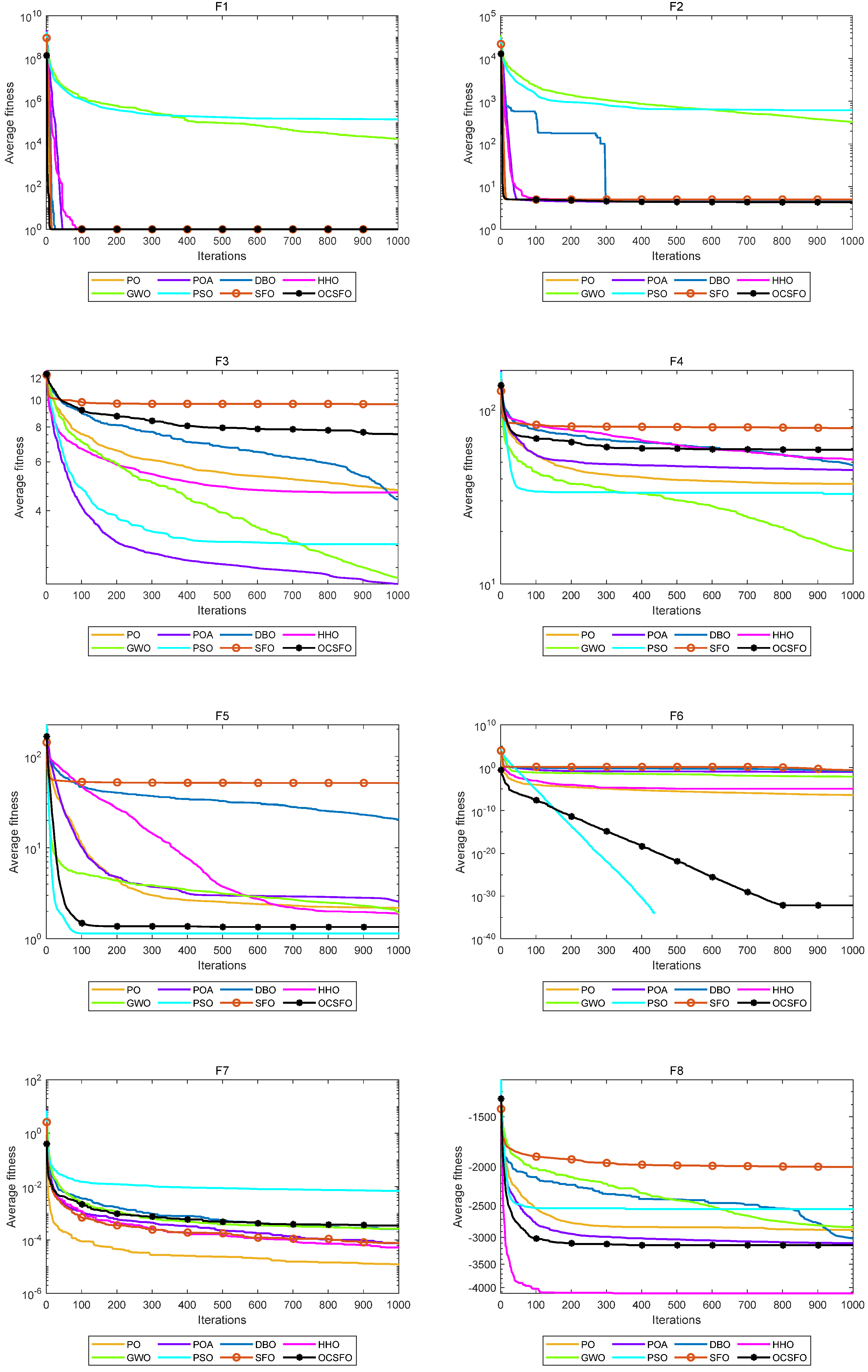
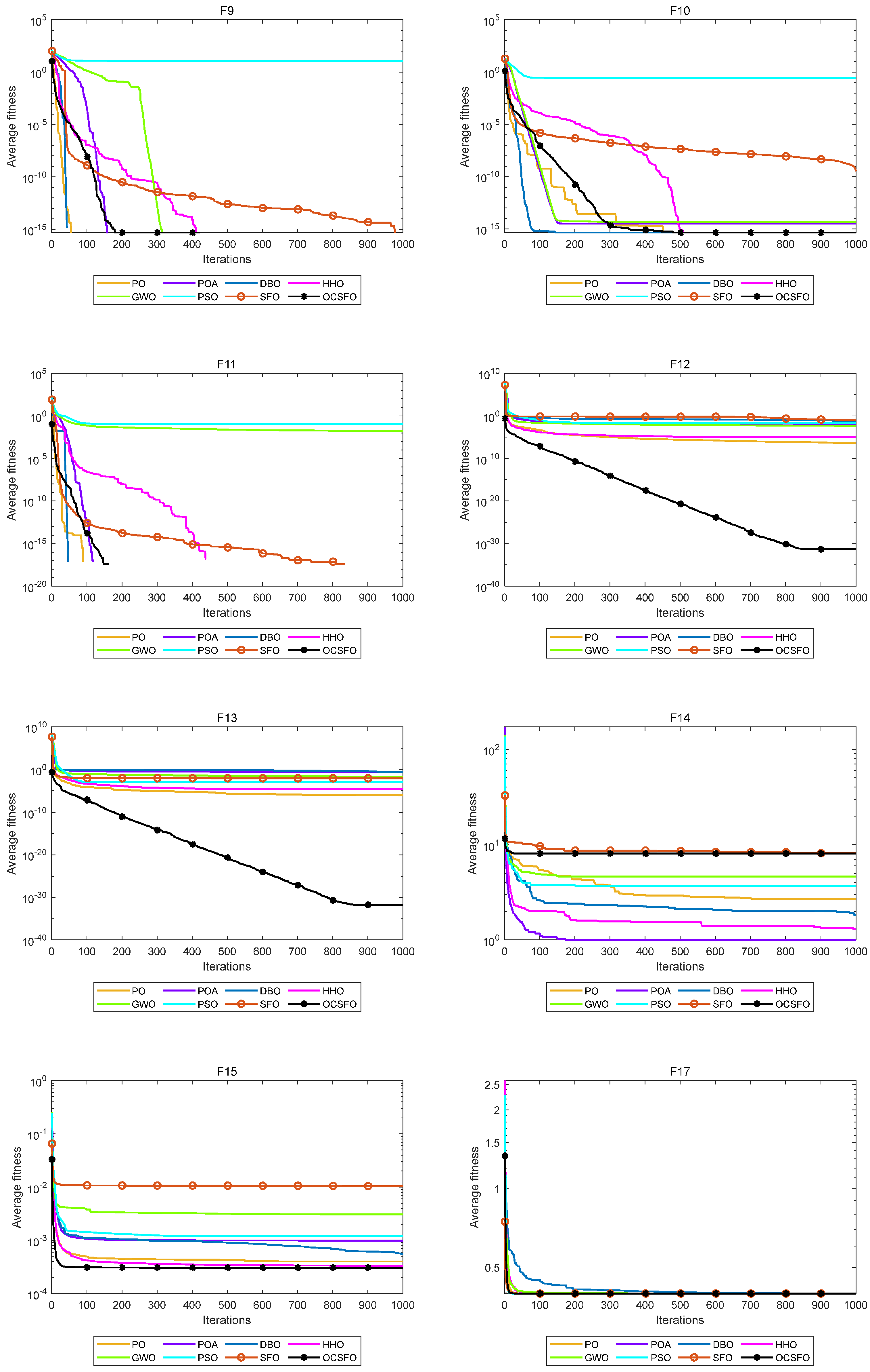
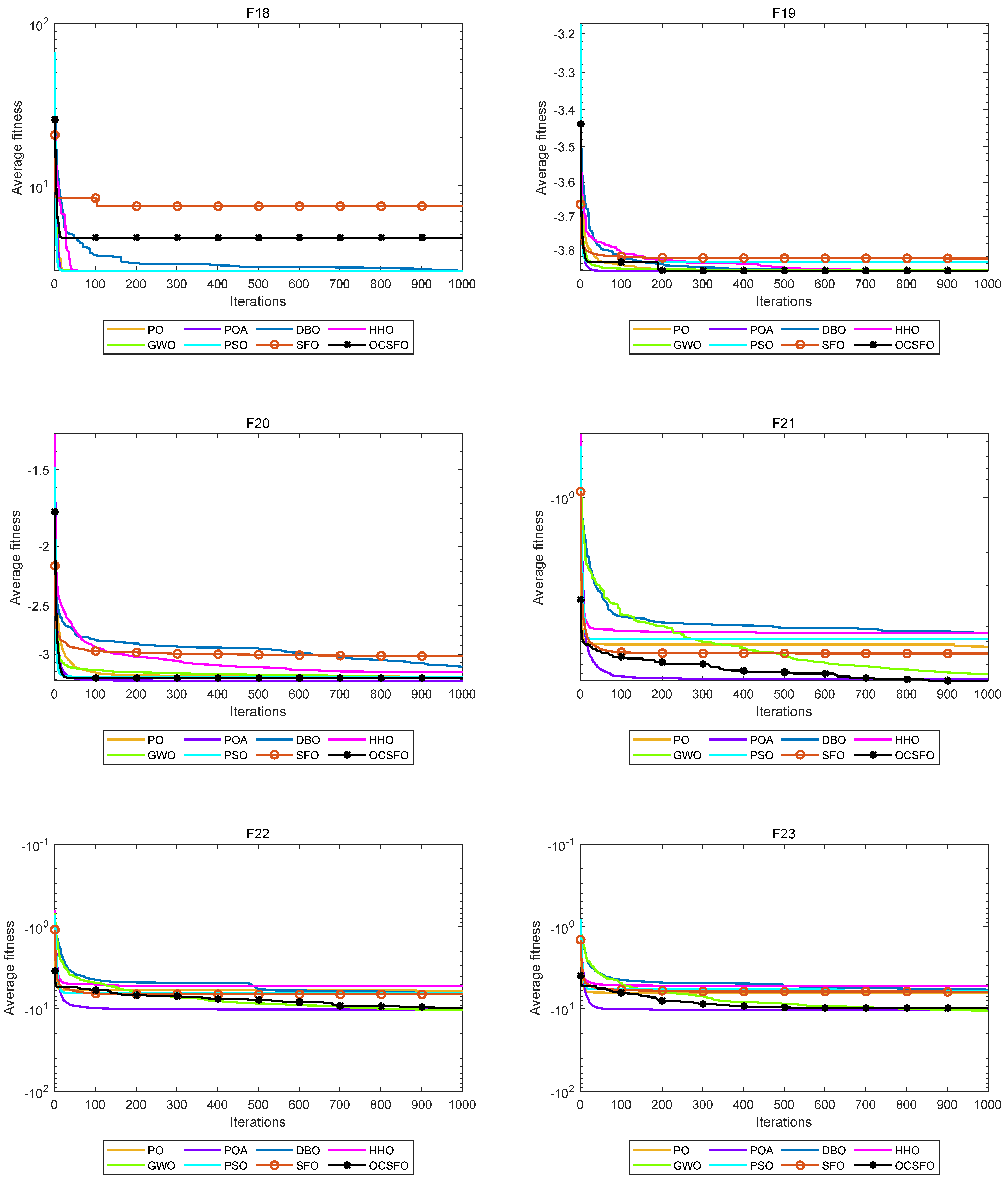
(3) Convergence Performance Analysis

To verify the convergence performance of the OCSFO algorithm, this experiment lists the comparison charts of the iterative convergence curves of the OCSFO algorithm and other intelligent optimization algorithms on 23 classic benchmark test functions. The name of the benchmark function is shown at the top of each comparison chart. The convergence curves of 8 comparison algorithms on the classic benchmark test functions are shown in Figure 2.

Comparison of 23 classical function radar charts for 8 algorithms is shown in Figure 3.

As illustrated in Figure 2 and Figure 3, OCSFO demonstrates superior convergence behavior by attaining better solutions in F1, F2, and F5, while closely approaching the theoretical optimal value in F6. For the unimodal functions F3 and F4, although OCSFO does not fully converge to the theoretical optimum, it still achieves substantial improvements in solution accuracy and convergence velocity when juxtaposed with the classical SFO algorithm. This highlights the effectiveness of its hybrid exploration-exploitation mechanism in gradient-based optimization landscapes.

Notably, OCSFO excels in multimodal function optimization. In F9, F10, F11, F12, and F13—characterized by complex, multi-peak structures—it not only converges to the theoretical optimal values but also does so with significantly faster convergence kinetics compared to other algorithms. This proficiency underscores its enhanced ability to navigate rugged fitness landscapes and avoid premature stagnation in local optima. Further validation is observed in fixed-dimension multimodal functions (F15, F17, F19, F20, F21, F22, F23), where OCSFO consistently exhibits stronger global search capabilities. Function F16 encountered an error and did not display the image, it is not be displayed. Its performance across these diverse problem classes demonstrates remarkable adaptability to highly non-linear, multi-peak search spaces, a critical advantage for real-world engineering applications.

Collectively, these results establish that OCSFO surpasses the classical SFO algorithm in both convergence speed and accuracy. When benchmarked against other state-of-the-art comparison algorithms, it demonstrates distinct dominance in handling multimodal and fixed-dimension multimodal challenges, showcasing robust escape mechanisms from local optima, superior convergence precision, and overall optimal performance. The findings solidify OCSFO’s utility as a versatile and efficient optimization framework for complex, high-dimensional problems in engineering and machine learning. In response to the problems of search ability, convergence speed, and local optima in the SFO benchmark algorithm, this paper proposes a swordfish optimization algorithm (OCSFO) that integrates the Osprey and Cauchy mutation. The first stage exploration strategy of the Osprey algorithm is used to improve the discoverer position update formula, increasing the exploration ability of SFO in identifying optimal regions and escaping local optima. The variable spiral update strategy and Cauchy mutation strategy are used to improve the follower update formula and dynamically update the target position. Through comparative analysis of experiments, the algorithm has shown significant improvements in convergence speed, convergence accuracy, probability of escaping local optima, and global search capability.

5.4. Engineering Problem Optimization Experiments

Solving practical engineering problems is one of the main applications of swarm intelligence algorithms. However, the results in test functions cannot fully reflect the application effect of the algorithm in practical problems. Engineering constraint optimization problems are widely used in various fields. Such problems usually revolve around aspects such as time, quality, and resource consumption. They optimize one or more objectives under a given engineering background while satisfying engineering constraint conditions, maximizing efficiency, minimizing costs, and balancing various indicators. This paper evaluates the practicality of OCSFO by solving four engineering problems: piston rod, three-bar truss, cantilever beam, and topology optimization.

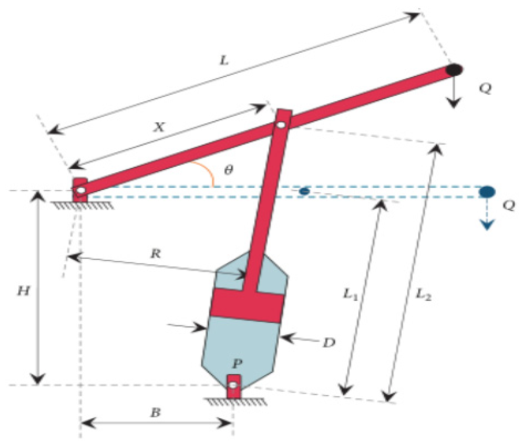
(1) Piston Rod Optimization

The main goal of the piston rod problem is to locate the piston components H(=x₁), B(=x₂), D(=x₃), X(=x₄) by minimizing the oil volume, as shown in Figure 4 [46].

The mathematical model of the piston rod design problem is expressed as follows:

(1) Objective Function:

$$f(x)={\displaystyle \frac{1}{4}}\pi x_3^2(L_2-L_1)$$

(19)

(2) Constraint Conditions:

$$g_1(x)=QL\cos \theta -R\times F\le 0$$

(20)

$$g_2(x)=Q(L-x_4)-M_{\max }\le 0$$

(21)

$$g_3(x)=1.2(L_2-L_1)-L_1\le 0$$

(22)

$$g_4(x)={\displaystyle \frac{x_3}{2}}-x_2\le 0$$

(23)

$$R={\displaystyle \frac{-\mid x_4(x_4\sin \theta +x_1)+x_1(x_2-x_4\cos \theta )\mid }{\sqrt{{\left(x_4-x_2\right)}^2+x_1^2}}}$$

$$F={\displaystyle \frac{\pi P{x}_3^2}{4}},L_1=\sqrt{{\left(x_4-x_2\right)}^2+x_1^2},L_2=\sqrt{{\left(x_4\sin \theta +x_1\right)}^2+{\left(x_2-x_4\cos \theta \right)}^2}$$

(3) Variable Range:

$$0.05\le x_1,x_2,x_4\le 500,0.05\le x_3\le 120$$

(4) Parameter Setting:

$$\theta ={45}^{°},Q=10000lbs,M_{\max }=1.8\times {10}^{6}lbsin,P=1500psi$$

The optimized results are shown in

Table 4. Comparison of Results of Piston Rod Design Problem.

Index	OCSFO	SFO	PSO	GWO	HHO	DBO	POA	PO
min	1.057393888	3.705359971	1.057393888	1.058252743	2.306290401	1.05806147	1.057393888	1.057803626
std	71.58905973	235.6597908	67.70409954	57.59179142	203.8252736	0.00994854	4.10374 × 10−12	0.047900342
avg	39.88763899	254.3648035	34.34046112	23.26917275	212.0547293	1.066258372	1.057393888	1.077079603
median	1.057393888	218.6506697	1.057393888	1.059041966	241.8198102	1.063558215	1.057393888	1.061981985
worse	167.4727301	916.011294	167.4727301	167.6960173	941.331882	1.104211354	1.057393888	1.252325321

.

It can be seen from Table 4, Figure 5 and Figure 6 that compared with the other seven algorithms, OCSFO can find the minimum optimization result of the piston rod problem. The optimal value obtained by OCSFO for the piston rod problem is 1.0574, and the optimal solution is x = [0.05, 1.0081, 2.0162, 500].

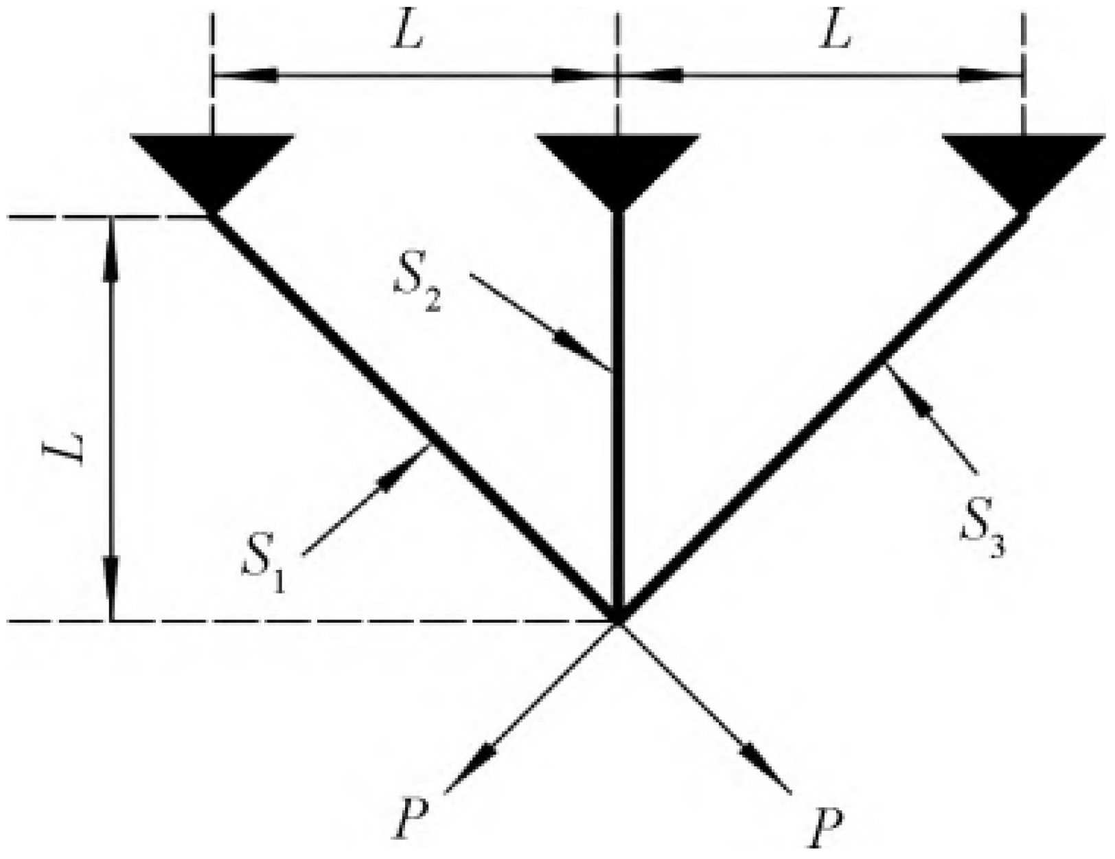
(2) Three-Bar Truss Optimization

As shown in Figure 7, the three-bar truss design problem (TBTD) is a problem involving optimization and constraint satisfaction. In the process of solving this problem, it is necessary to adjust two key parameters S₁ and S₂ to achieve the minimum weight of the truss while satisfying 3 specific constraint conditions [47].

The mathematical model of the three-bar truss design problem is expressed as follows:

(1) Objective Function:

$$f(x)=(2\sqrt{2S_1}+S_2)\times L$$

(24)

(2) Constraint Conditions:

$$g_1(x)={\displaystyle \frac{\sqrt{2}{S}_1+S_2}{\sqrt{2}{S}_1^2+2S_1{S}_2}}P-\sigma ⩽0$$

(25)

$$g_2(x)={\displaystyle \frac{S_2}{\sqrt{2}{S}_1^2+2S_1{S}_2}}P-\sigma ⩽0$$

(26)

$$g_3(x)={\displaystyle \frac{1}{\sqrt{2}{S}_2+S_1}}P-\sigma ⩽0$$

(27)

(3) Variable Range:

$$0⩽S_1,S_2⩽1$$

(4) Parameter Setting:

$$L=100 \mathrm{cm},P=2 {\mathrm{kN}/\mathrm{cm}}^2,\sigma =2 {\mathrm{kN}/\mathrm{cm}}^2$$

The optimized results are shown in

Table 5. Comparison of Results of Three-Bar Truss Design Problem.

Index	OCSFO	SFO	PSO	GWO	HHO	DBO	POA	PO
min	263.8958439	263.8964172	263.8958446	263.8961538	263.8958438	263.8989862	263.8958434	263.8960476
std	0.003160076	0.978514267	0.012579509	0.002963536	0.082994899	0.143038184	1.73446 × 10−13	0.064466374
avg	263.8974988	264.2162079	263.8994882	263.8995972	263.9630128	263.9922193	263.8958434	263.9546643
median	263.8963985	263.9013246	263.8963453	263.8985967	263.9235141	263.9434366	263.8958434	263.9328776
worse	263.912221	268.2329229	263.9649984	263.9104325	264.2055554	264.5910234	263.8958434	264.1468713

.

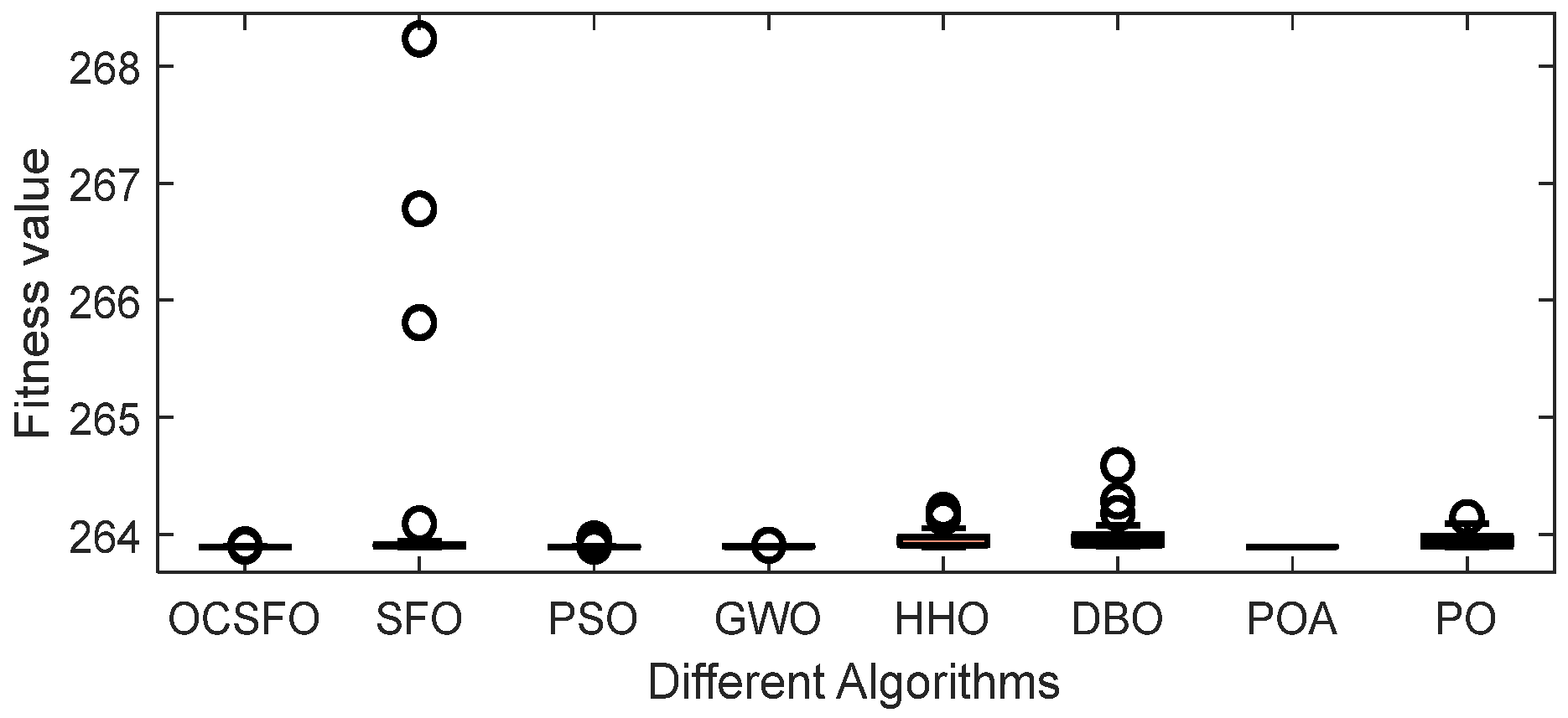
It can be seen from Table 5, Figure 8 and Figure 9 that compared with the other seven algorithms, OCSFO can find a result close to the minimum optimization of the three-bar truss design problem. The optimal value obtained by OCSFO for the piston rod problem is 263.8958, and the optimal solution is s = [0.7887, 0.4082].

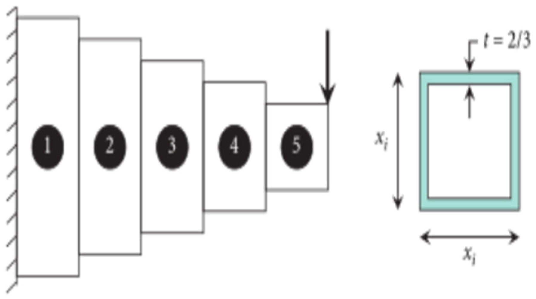
(3) Cantilever Beam Optimization

The cantilever beam problem is a structural engineering design example involving the weight optimization of a rectangular-cross-section cantilever beam. One end of the beam is rigidly supported, and the free node of the cantilever is subjected to a vertical force, as shown in Figure 10. The beam consists of 5 hollow squares with a constant thickness. The height (or width) of the square is the decision variable, and the thickness remains fixed [48].

The mathematical model of the cantilever beam design problem is expressed as follows:

(1) Objective Function:

$$f(x)=0.0624(x_1+x_2+x_3+x_4+x_5)$$

(28)

(2) Constraint Conditions:

$$g(x)={\displaystyle \frac{61}{x_1^3}}+{\displaystyle \frac{37}{x_2^3}}+{\displaystyle \frac{19}{x_3^3}}+{\displaystyle \frac{7}{x_4^3}}+{\displaystyle \frac{1}{x_5^3}}-1\le 0$$

(29)

(3) Variable Range:

$$0.01\le x_i\le 100,i=1,\dots ,5$$

The optimized results are shown in

Table 6. Comparison of Results of Cantilever Beam Design Problem.

Index	OCSFO	SFO	PSO	GWO	HHO	DBO	POA	PO
min	1.339958663	1.392375298	1.339964106	1.339967494	1.340324097	1.339988698	1.339957158	1.339974185
std	4.94849 × 10−5	0.073503549	8.33206 × 10−5	5.36225 × 10−5	0.001782612	0.000187978	2.06533 × 10−5	0.001696178
avg	1.340013375	1.562350216	1.340028467	1.340029792	1.343013401	1.340224839	1.339980581	1.342146539
median	1.339998765	1.569603889	1.339999659	1.340011161	1.342809025	1.340188156	1.339975646	1.341582181
worse	1.340181508	1.715542068	1.340359248	1.340201323	1.346352002	1.340711677	1.340043744	1.346670449

.

It can be seen from Table 6, Figure 11 and Figure 12 that compared with the other seven algorithms, OCSFO can find a result close to the minimum optimization of the cantilever beam design problem. The optimal value obtained by OCSFO for the cantilever beam design problem is 1.33996, and the optimal solution is x = [6.0082, 5.3148, 4.49383, 3.5022, 2.1548].

(4) Topology Optimization

The main purpose of the topology optimization problem is to optimize the material layout of a set of provided loads within a given design search space and under constraint conditions related to system performance. This problem is based on the power-law method, and its mathematical model is expressed as follows [49]:

(1) Objective Function:

$$f(\overline{x})=U^{T}KU={\displaystyle \sum _{e=1}^N{(x_e)}^p}{u}_e^T{k}_0{u}_0$$

(30)

(2) Constraint Conditions:

$$h_1(\overline{x})={\displaystyle \frac{V(\overline{x})}{V_0}}-f=0$$

(31)

$$h_2(\overline{x})=KU-F=0$$

(32)

(3) Variable Range:

$$0<{\overline{x}}_{min}\le x\le 1$$

The optimized results are shown in

Table 7. Comparison of Results of Topology Optimization Problem.

Index	OCSFO	SFO	PSO	GWO	HHO	DBO	POA	PO
min	2.639346497	2.639346497	2.65060516	2.749913511	2.639346497	2.639346497	2.639346497	2.639346497
std	0	0	0.120402243	0.106492184	0	0	0.423009132	0
avg	2.639346497	2.639346497	2.798178306	2.885364818	2.639346497	2.639346497	3.05899145	2.639346497
median	2.639346497	2.639346497	2.755642485	2.847282767	2.639346497	2.639346497	2.94908224	2.639346497
worse	2.639346497	2.639346497	3.1143788	3.173423754	2.639346497	2.639346497	4.366127615	2.639346497

.

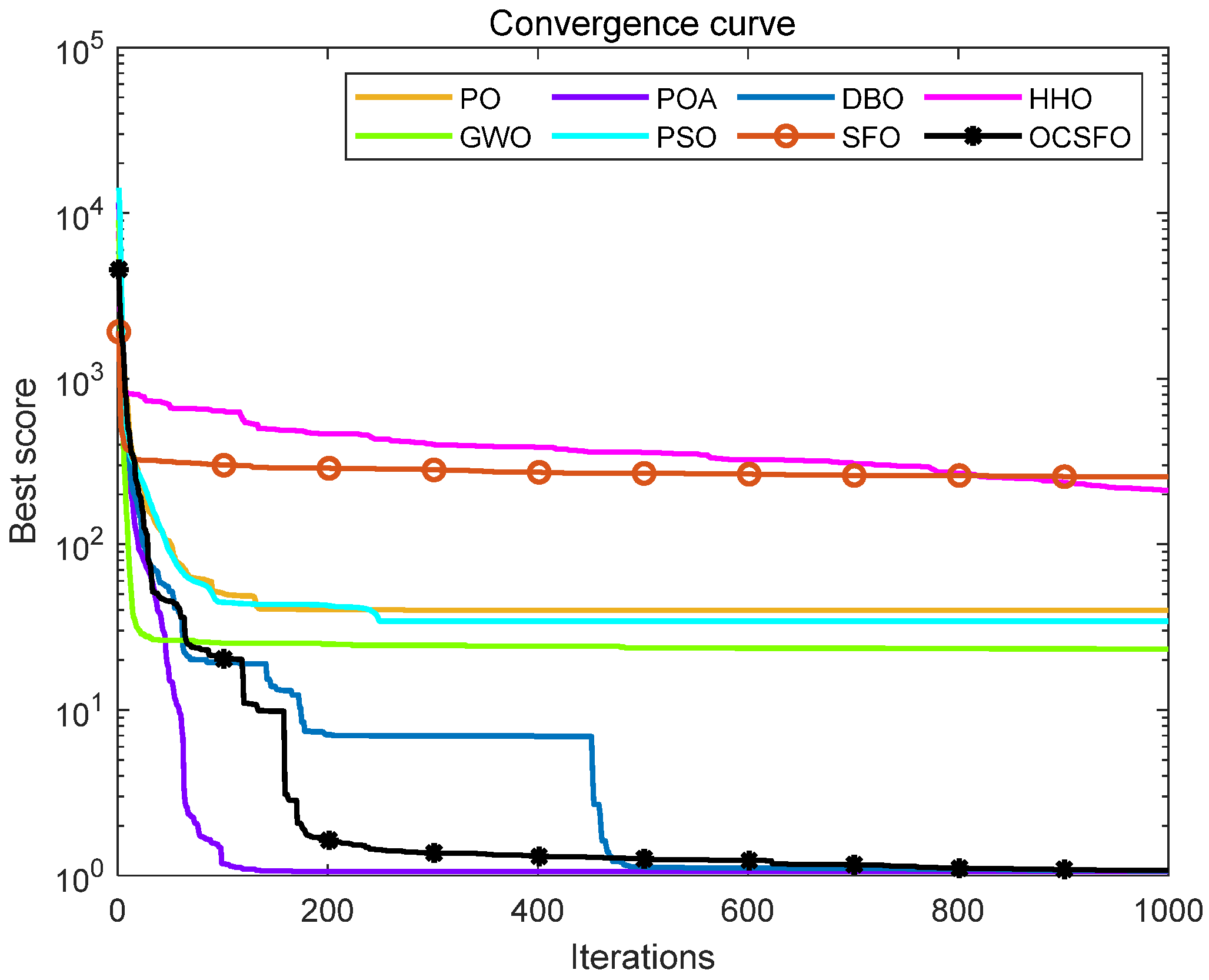
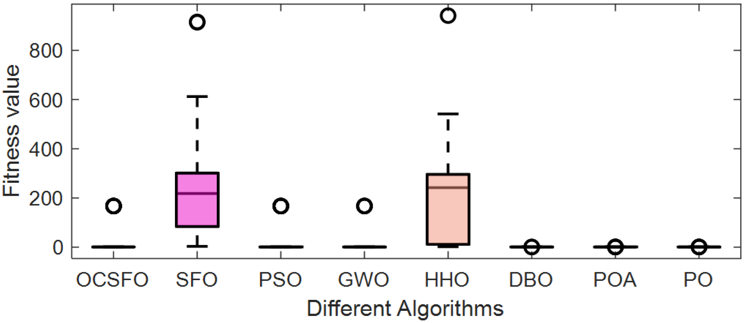
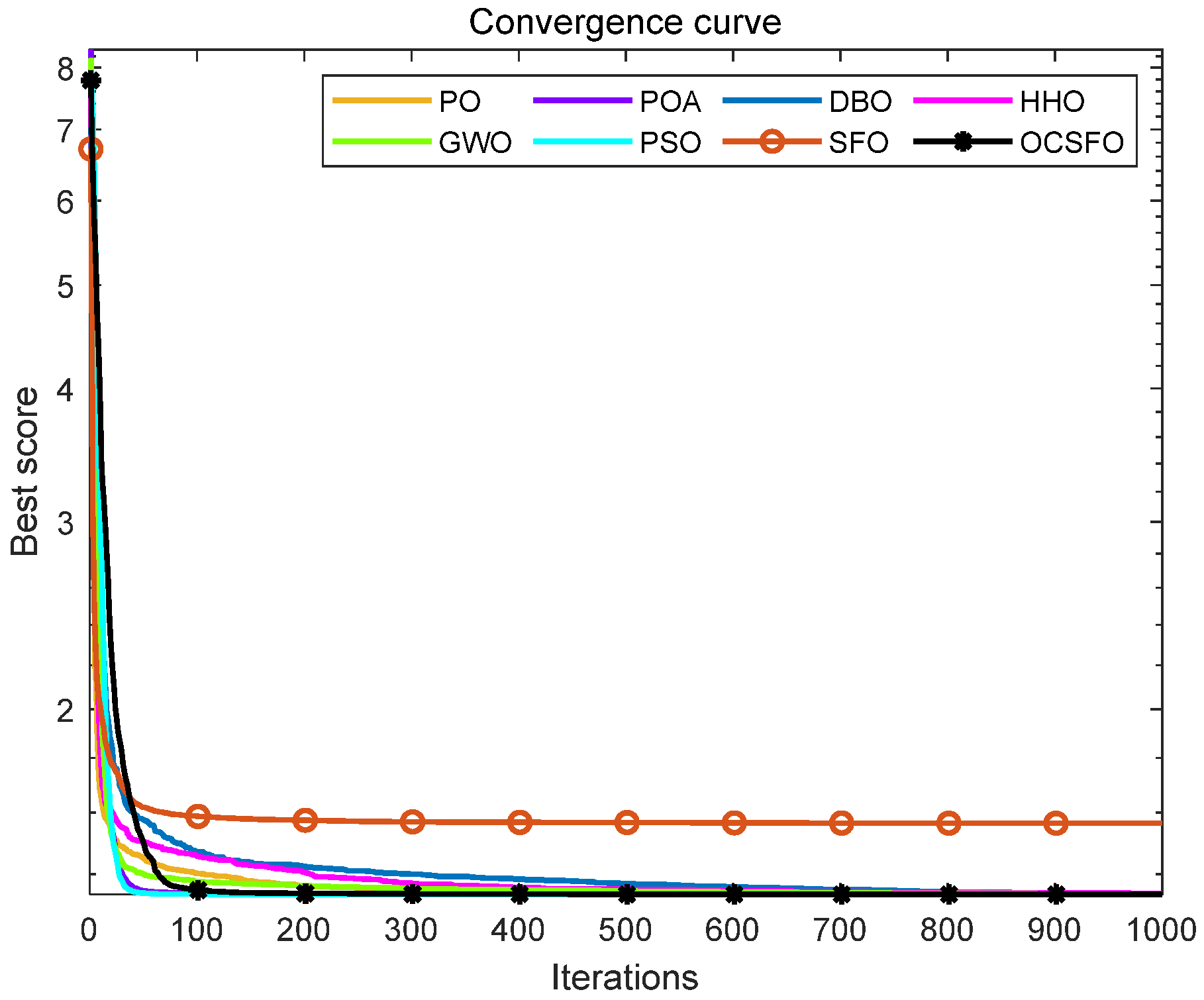
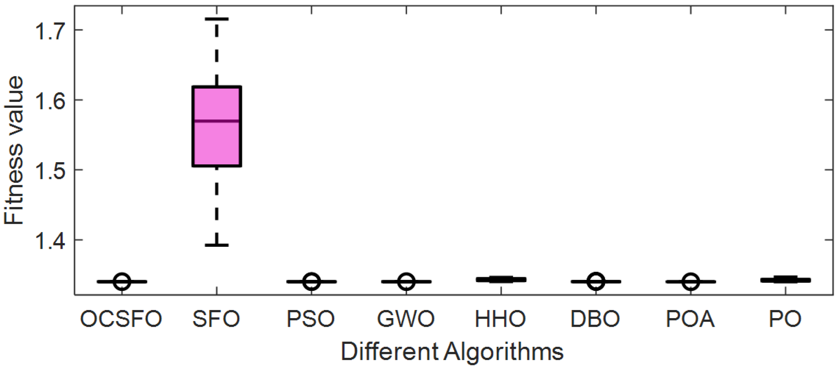
The average convergence curve of topology optimization problem is shown in Figure 13. The box plot of topology optimization problem is shown in Figure 14.

It can be seen from Table 7, Figure 13 and Figure 14 that compared with the other seven algorithms, OCSFO can find a result close to the minimum optimization of the topology optimization problem. The optimal value obtained by OCSFO for the topology optimization problem is 2.6393.

From the comparison of four engineering application algorithms, the optimal value of the OCSFO algorithm ranks first compared to the seven comparison algorithms, indicating that OCSFO has good optimization ability in solving design problems of piston rods, three bar trusses, cantilever beams, and topology optimization. Compared with the SFO algorithm, it can be seen that the proposed OCSFO has an enhanced ability to jump out of local optima. Under the fusion of the Fishhawk and Cauchy mutation, its optimization accuracy is high, the optimization speed is fast, and the stability is strong.

6. Conclusions

The Osprey and Cauchy Mutation Integrated Sailfish Optimization Algorithm (OCSFO) proposed in this paper effectively improves and enhances the optimization performance of the Sailfish Optimization Algorithm (SFO). (1) The sailfish and sardine populations are initialized using the Logistic map. (2) The global exploration strategy of the Osprey Optimization Algorithm in the first stage is adopted during the local development phase of sailfish individual position update to enhance the global search ability of the algorithm. (3) Cauchy mutation is introduced to stimulate the activity of the sailfish and sardine populations during the prey capture stage. Through experimental verification, in the process of solving 23 classic benchmark test functions, the convergence speed, optimization accuracy, and robustness of OCSFO have been significantly improved. At the same time, the results of OCSFO in solving 4 complex engineering design optimization problems show that it has good applicability and superior solution effects in dealing with different types of practical complex optimization problems. In future research, further studies can be carried out on applying the OCSFO algorithm to multi-objective optimization problems.