Article

Video Stabilization Algorithm Based on View Boundary Synthesis

by
Wenchao Shan
1,2,
Hejing Zhao
3,4,
Xin Li
1,2,*,
Qian Huang
1,2,*,
Chuanxu Jiang
2,
Yiming Wang
2,
Ziqi Chen
5 and
Yao Tong
1,6
1
Jiangsu Engineering Research Center of Digital Twinning Technology for Key Equipment in Petrochemical Process, Changzhou University, Changzhou 213164, China
2
College of Computer Science and Software Engineering, Hohai University, Nanjing 210098, China
3
Research Center on Flood and Drought Disaster Reduction of Ministry of Water Resource, China Institute of Water Resources and Hydropower Research, Beijing 100038, China
4
Water History Department, China Institute of Water Resources and Hydropower Research, Beijing 100038, China
5
Department of Earth System Science, Tsinghua University, Beijing 100084, China
6
School of Artificial Intelligence and Information Technology, Nanjing University of Chinese Medicine, Nanjing 210023, China
*
Authors to whom correspondence should be addressed.
Symmetry 2025, 17(8), 1351; https://doi.org/10.3390/sym17081351
Submission received: 11 June 2025 / Revised: 23 July 2025 / Accepted: 5 August 2025 / Published: 19 August 2025
(This article belongs to the Special Issue Symmetry/Asymmetry in Image Processing and Computer Vision)

Abstract

Video stabilization is a critical technology for enhancing visual content quality in dynamic shooting scenarios, especially with the widespread adoption of mobile photography devices and Unmanned Aerial Vehicle (UAV) platforms. While traditional digital stabilization algorithms can improve frame stability by modeling global motion trajectories, they often suffer from excessive cropping or boundary distortion, leading to a significant loss of valid image regions. To address this persistent challenge, we propose the View Out-boundary Synthesis Algorithm (VOSA), a symmetry-aware spatio-temporal consistency framework. By leveraging rotational and translational symmetry principles in motion dynamics, VOSA realizes optical flow field extrapolation through an encoder–decoder architecture and an iterative boundary extension strategy. Experimental results demonstrate that VOSA enhances conventional stabilization by increasing content retention by 6.3% while maintaining a 0.943 distortion score, outperforming mainstream methods in dynamic environments. The symmetry-informed design resolves stability–content conflicts and outperforms mainstream methods in dynamic environments, establishing a new paradigm for full-frame stabilization.

1. Introduction

The widespread adoption of mobile photography devices and UAV platforms has positioned video stabilization as a critical technology for enhancing visual content quality. In dynamic shooting scenarios, traditional physical stabilization systems often fail to fully eliminate high-frequency jitters, whereas digital video stabilization algorithms based on motion estimation and compensation can effectively improve frame stability by modeling global motion trajectories [1,2]. However, existing methods frequently suffer from excessive cropping or boundary distortion during stabilization, leading to a significant loss of valid image regions—a phenomenon that not only reduces video resolution but may also compromise essential visual information.
This issue is particularly prominent in professional cinematography and mobile video applications: aggressive cropping disrupts directors’ compositional intent, while boundary warping causes deformations of moving objects. Although optical flow–sensor fusion methods have advanced motion estimation accuracy, their inherent reliance on frame warping inevitably introduces boundary cropping artifacts. Consequently, developing stabilization algorithms that preserve original frame integrity has become an urgent challenge in computer vision research.
To address the significant cropping artifacts inherent in warping-based stabilization methods, we propose a novel view-outpainting algorithm for boundary synthesis. Building upon the spatio-temporal continuity and inherent symmetry properties of video motion [3,4], our approach intelligently completes missing boundary pixels caused by stabilization, effectively minimizing content loss. Specifically, by deeply exploiting inter-frame motion consistency (translational symmetry) and intra-frame spatial coherence (rotational symmetry), the method establishes precise pixel-wise correspondences while preserving structural symmetry to achieve high-quality view boundary extrapolation. The key contributions of this work include a symmetry-aware framework, a lightweight network architecture, and a mathematical model for motion propagation, all of which are validated through extensive experiments.
From the perspective of technical implementation, we adopt a three-stage processing flow. First, an accurate optical flow field [5,6] is calculated using a global optimization framework that incorporates affine motion symmetry. Subsequently, based on the motion affinity metric that respects motion symmetry, the flow field is extended to the area outside the view boundary to generate sufficient sampling points. Finally, adaptive pixel warping [7] is performed under symmetry constraints. It is noteworthy that this symmetry-aware solution features a modular architecture, allowing seamless integration into existing video stabilization frameworks that combine optical flow and sensor fusion. This integration effectively minimizes cropping in the stabilized output videos.
In summary, our contributions are as follows:
  • We propose the View Out-boundary Synthesis Algorithm (VOSA) grounded in spatio-temporal coherence and symmetry principles. This algorithm accomplishes the completion of missing pixels via symmetry-preserving optical flow extension and an iterative propagation mechanism.
  • We design a lightweight network architecture that can be seamlessly integrated into existing video stabilization pipelines. Through the coordinated operation of the pre-alignment module and the affinity kernel prediction network, this architecture boosts the cropping rate of classic algorithms like MeshFlow [8] by 12.3% without incurring a computational overhead increase of more than 5%.
  • We establish a mathematical representation model for symmetry-aware motion propagation across video frames. It is theoretically demonstrated that the optical flow field beyond the boundary can be linearly approximated by local affinity kernels satisfying symmetry constraints.
The rest of this paper is organized as follows: Section 2 reviews related works on video stabilization. Section 3 details the methodology of our proposed VOSA algorithm. Section 4 presents experimental results and comparisons with state-of-the-art methods. Finally, Section 5 concludes the paper and discusses future directions.

2. Related Works

Traditional digital video stabilization algorithms have evolved through multiple innovative approaches. Grundmann [9] pioneered an L1 optimization framework, generating smooth camera paths adhering to cinematographic principles by minimizing derivatives under linear programming constraints. This method effectively eliminated low-frequency jitter by producing derivative-free segments. Building on this, Bradley [10] introduced homography transformations rooted in Lie theory, operating in logarithmic homography space to maintain linearity and employing L2-norm constraints for path approximation, while enforcing the validity of cropped pixels through area and perimeter constraints. Liu proposed SteadyFlow [11], which stabilized videos by smoothing optical flow fields, initialized them using hybrid traditional–global matrices, and segmented motion vectors via spatio-temporal analysis. Further refinement led to MeshFlow [8], an online method with single-frame latency, utilizing dynamic buffers and sliding windows to ensure path continuity. Zhang [1] accelerated stabilization via joint trajectory optimization for de-jittering and mesh warping, while their work [12] leveraged Riemannian metrics in Lie groups to derive geodesic-based paths for geometric interpolation. Wu [13] addressed motion heterogeneity using motion-steering kernels and low-rank regularization, overcoming the isotropic limitations of Gaussian kernels. Zhao and Ling [1] mitigated foreground loss through similarity constraints on Delaunay triangulated meshes, enforcing geometric consistency across frames. Zhang [14] proposed a high-precision video stabilization method (VSM) based on ED-RANSAC, an error elimination operator constrained by Euclidean distance, and sorted out a set of accuracy evaluation methods. Jang [15] proposed a hybrid full-frame video stabilization algorithm, integrating IMU sensor data with the Versatile Quaternion-based Filter and optical flow to perform motion compensation, PCA-flow stabilization, and neural rendering for distortion mitigation.
While traditional methods provide an important foundation for video stabilization, their reliance on constrained distortion operations or computationally intensive registration techniques inevitably compromises video stabilization. Figure 1 shows that warping-based video stabilization methods achieve camera path smoothing by constraining pixel displacement, mapping unstable input frames to stabilized ones. These approaches face inherent limitations in that the stabilized pixels are queried from the initial frames via transformation matrices, yet the initial frames often provide an insufficient field-of-view, resulting in missing pixels. As shown in Figure 2, to maintain visual coherence, conventional methods inevitably crop stabilized frames, causing reduced output resolution, aspect ratio distortion, or even amplified jitter. This creates a trade-off situation between stability and content preservation. To enhance stability, one has to sacrifice visual content; conversely, retaining content is likely to lead to a decline in stabilization performance.
In recent years, deep learning-based methods [16,17,18] have shown great potential in image data processing. Zhao [19] proposed PWStableNet, a deep learning-based pixel-wise video stabilization network, utilizing a multi-stage cascade encoder–decoder architecture with inter-stage connections to generate per-pixel warping maps for stabilized views, achieving robustness to parallax and improved processing speed. Yu [20] proposed a novel neural network that infers per-pixel warp fields from optical flow, coupled with a pipeline using optical flow principal components for motion inpainting and warp smoothing, achieving robustness to moving objects/occlusion. Xu [21] proposed DUT, an unsupervised deep video stabilization framework combining the traditional divide-and-conquer strategy with deep neural networks. It employs multi-homography motion refinement for trajectory estimation and dynamic kernel-based trajectory smoothing, eliminating the need for paired training data while outperforming state-of-the-art methods.
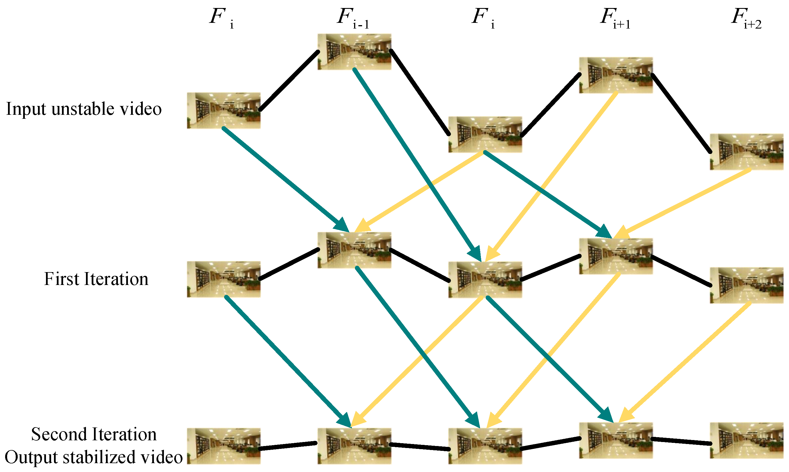
For stabilization of the full frame, Choi and Kweon proposed DIFRINT [22], generating intermediate frames through interpolation of the adjacent frames (Figure 3). The method follows the principle of spatial correlation, and its core idea has been validated in the fields of structure in motion restoration (SFM) [23,24], video restoration [25,26,27], and super-resolution [28,29,30]. However, traditional warping methods rarely utilize this property to complement out-of-boundary pixels.
Image registration provides an alternative solution. Classical methods rely on feature detectors, such as SIFT [31], SURF [32], ORB [33], and LIFT [33], in combination with RANSAC [23], for outlier rejection (Figure 4). At the same time, deep learning-based alignment methods, trained through either supervised or unsupervised paradigms, have shown excellent performance in modeling complex spatial transformations [34,35,36]. Although they are promising in achieving a balance between quality and content, their real-time applicability and generalization still face challenges. In contrast, our proposed video out-scaling stabilization algorithm (VOSA) overcomes the dual limitations of previous approaches and establishes a new paradigm for full-frame video stabilization.

3. Methodology

3.1. Overview

The algorithm elaborated in this paper is dedicated to fully exploring the continuity in the temporal dimension and the spatial correlation of the video sequence, so as to mitigate the cropping effects generated during the warping process and thus present a more complete and stable visual effect. To achieve this goal, the method adopted in this paper utilizes the pixel information of adjacent frames to expand the out-of-boundary view of the current frame. This expansion operation not only provides convenient conditions for obtaining stable frames through image warping in the subsequent process, but more crucially, it can efficiently locate and determine a set of candidate pixels that are indispensable for generating full-frame stable frames.
The View Out-boundary Synthesis Algorithm (VOSA) proposed in this paper first performs a pre-alignment operation on the input frames to obtain a pre-aligned frame sequence. Subsequently, by means of the optical flow field information calculated by FlowNet2, the Affinity Propagation (AP) clustering algorithm is used to predict the distribution of the optical flow field of the out-of-boundary view of the frame. Based on these predicted optical flow field data, the algorithm performs warping processing on the pixels in adjacent frames, and the specific process is shown in Figure 5 in detail. This process can be carried out iteratively, gradually aligning adjacent frames that are farther from the current frame with the current frame, thus continuously expanding the scope of the out-of-boundary view. In this way, the subsequent image warping process can more efficiently locate and acquire the required candidate pixels, and then generate more complete and stable video frames.
Specifically, the affine transformation matrix is estimated by first computing the optical flow between consecutive frames using the FlowNet2 model. The optical flow provides pixel-wise displacement information, capturing motion dynamics between frames. To estimate the transformation matrix, we use the optical flow field to predict affinity kernels, which model local pixel motion based on the flow information. These affinity kernels allow us to perform a local affine transformation, ensuring accurate alignment between the frames.
Once the affinity kernels are predicted, we compute the transformation matrix by solving for the optimal affine parameters that minimize the difference between corresponding pixels in the aligned frames. This is performed using a least-squares optimization, which iteratively refines the transformation matrix to reduce misalignments. The optimization process ensures that the matrix accounts for the spatial coherence of the image, preserving the geometric integrity of the scene.
To address lens distortions, which introduce nonlinearity and uncertainty into the affine transformation, we apply a lens distortion correction model prior to calculating the optical flow. This step corrects radial and tangential distortions, ensuring that the image geometry is accurate before estimating the transformation matrix. This correction improves the robustness of the transformation, especially in cases where the camera lens introduces significant distortion.
However, the optical flow computed by FlowNet2 is based on deep learning approximations, which can introduce some uncertainty. While the model generally provides accurate displacement estimates, errors can occur in regions of rapid motion, occlusions, or low-texture areas. We quantify the uncertainty of the optical flow by comparing it against ground truth data and use a robust optimization strategy to minimize the impact of outliers during matrix estimation. This ensures that the final affine transformation is both accurate and stable.

3.2. Frame Boundary Processing

To address this problem of large cropping in previous algorithms, VOSA takes as input a sequence of video frames, F i | i = 1 , , n , where n represents the total number of video frames and F i denotes the ith frame in that video. The size of the input frame F i is denoted as H 0 × W 0 . In order to optimize the processing effect, we adopt a zero-filling strategy beyond the four boundaries of each frame. We uniformly add 80 pixels to the filling region in each direction. The size of the buffer is directly related to the maximum frequency and amplitude of the vibrations expected in the video. Since high-frequency vibrations result in rapid motion, a larger buffer ensures that the algorithm can account for such movements without losing critical information. In practice, 80 pixels are found to be a balanced trade-off between computational efficiency and motion compensation accuracy, as larger buffers could result in unnecessary computational overhead without providing significant additional benefit. The chosen buffer size also relates to the resolution required for streaming compensation. By ensuring that the border is large enough, we maintain the necessary spatial information in the extended region for accurate boundary estimation. The 80-pixel buffer effectively provides enough room for the optical flow field to extrapolate beyond the frame boundary, helping the algorithm maintain content integrity and minimize cropping artifacts during stabilization.
At the same time, a mask sequence M i | i = 1 , , n is introduced to denote the effective frame region after padding. In this way, the video frames output from the previous algorithm can be converted into an input format more suitable for frame alignment processing.
After completing the above pre-processing operations on the input frames, we further employ the SIFT feature point detection algorithm to identify the key feature points and filter the robust feature point set by the RANSAC algorithm. Subsequently, we compute the single responsiveness matrix corresponding to the feature points in each frame to achieve the initial alignment of the input frames. In this step, the set of input data required for the subsequent frame boundary expansion network is obtained,
{ F ^ i i + 1 , M ^ i i + 1 i = 1 , , n } { F ^ i i 1 , M ^ i i 1 i = 1 , , n }
where the first set of data denotes the queue of pre-aligned frames and masks that are passed from the current frame to the subsequent one, and the latter group represents the corresponding information queue passed from the current frame to the previous frame. Such a bidirectional delivery strategy is adopted to ensure the coherence and accuracy of inter-frame alignment.
In the implementation of SIFT, default parameters were adopted for all stages. Among the key parameters configured, the contrast threshold was set to 0.04. This value was selected to balance the sensitivity of keypoint detection in low-contrast regions, ensuring an adequate number of keypoints are identified while mitigating the inclusion of excessive noise in the feature set. The edge threshold, configured to 10, functions to filter out keypoints situated on edges or those with poor localization, thereby retaining only stable and repeatable keypoints. Additionally, 4 octaves were employed to cover a broad range of scales, facilitating keypoint detection across varying image resolutions and proving particularly advantageous for videos characterized by diverse motion patterns. For RANSAC, which is tasked with removing outliers in feature correspondences between consecutive frames, several key parameters were specified. The distance threshold was set to 5 pixels, a value that provides sufficient tolerance for potential misalignments while preserving the robustness of feature correspondences.Furthermore, an inlier ratio threshold of 0.8 was applied, mandating that at least 80% of the selected feature matches align with the derived model; this criterion guarantees the stability and accuracy of the frame alignment process. These parameter settings enable the stabilization process to handle dynamic content while maintaining high-quality output.
Among them, F ^ n n + 1 = F n , M ^ n n + 1 = M n , F ^ 1 0 = F 1 , and M ^ 1 0 = M 1 . After the pre-alignment process, we notate the uniform dimensions of the obtained pre-aligned frames and their corresponding masks as H m × W m to facilitate subsequent processing and analysis. To simplify the presentation, we abbreviate F ^ i i + 1 and M ^ i i + 1 as F ^ i and M ^ i , respectively.
By using the FlowNet2 model [37] with { F ^ i 1 , F i } as the input data, the optical flow O p i i 1 between { F ^ i 1 , F i } is,
O p i i 1 = FlowNet ( F i , F ^ i 1 ) M i
where ⊙ stands for the element-by-element multiplication of the matrix.
Subsequently, we employ a Flow Reversal (FR) layer to compute the backward optical flow field between the reference frame F ^ i 1 and the current frame F i ,
( O p ˜ i 1 i , M ˜ i ) = FR ( O p i i 1 , M i ) F ^ i 1
The reason why FR is chosen to compute the reverse optical flow instead of using FlowNet2 directly is that the inclusion of some pixels in F ^ i 1 may correspond to pixels outside the view boundary of the current frame F i , which can lead to errors in the optical flow computed directly by it. In addition, the FR layer can reverse the output mask M i ˜ , a property that makes it more compatible with the needs when dealing with pixel correspondences in the algorithms of this chapter. With the application of the FR layer, we are able to obtain the reverse optical flow information between { F ^ i 1 , F i } more accurately in order to improve the accuracy and reliability of our algorithm.
We utilized the optical flow within the shared view between two frames based on { F ^ i 1 , F i } to not only acquire the optical flow within the frame boundary but also further extrapolate the pixels outside the F i frame boundary. This is based on the spatial coherence property (SCP) within a frame, which means that the motion of a stationary object within an image is coherent in the local range. Based on this property, we accurately estimate the affinity kernels (AFs) by combining the color and structural information within the frame image. Subsequently, the affinity kernels are utilized to efficiently propagate the optical flow within the shared view outside the frame boundaries, thus enabling the estimation of the optical flow for the extended frame. A demonstration of the process is shown in Figure 6.

3.3. Network Infrastructure

After efficiently propagating the optical flow within the shared view beyond the frame boundaries through these affinity kernels, we utilize a codec-structured neural network to accurately predict the AF and the data flow and subsequent propagation computations for this network. As shown in Figure 7, the network uses F i , F ^ i 1 , M i , M ^ i 1 , M ˜ i , O p ˜ i 1 i , G i , and G ^ i 1 as inputs aiming at predicting affine kernel AFs, where G i , G ˜ i 1 are extracted by applying Sobel filters from the edge detection of F i , F ˜ i 1 . The Sobel filter can efficiently encode structural information in an image such as object edges and discontinuous regions and it extracts the edges by finding the pixel points bordering the regions in the image that have significant changes in brightness. The Sobel filter looks for the parts of the image that have significant changes in the gradient. These gradients are generally described as the amplitude and direction of the edges. By selecting pixels with high edge amplitude, we are able to clearly outline the edges of the region. This rich input data provides comprehensive information for the network and helps to predict the affinity kernel AF more accurately.
We use Sobel operators for edge detection, which are applied to the input frames to extract structural information and highlight high-frequency changes in the image. The Sobel operator is particularly effective for detecting edges, as it emphasizes regions with significant changes in intensity, such as object boundaries or other discontinuities in the image. The dimensions of the Sobel filter used are 3 × 3, which is commonly employed for detecting edges at various scales, while still maintaining computational efficiency. The 3 × 3 filter targets high-frequency components of the image, specifically those corresponding to rapid changes in pixel intensity along the horizontal and vertical directions.
The choice of a 3 × 3 Sobel filter is directly tied to the resolution of the image, as it is designed to capture edge information at a relatively fine scale. In high-resolution images, the Sobel operator effectively captures edge details without introducing excessive noise or computational complexity. For lower-resolution images, the filter’s dimensions and its ability to capture high-frequency content are sufficient to highlight the main structural features, allowing the network to focus on the essential boundaries without being overly sensitive to fine details.
We use ResNet-50 [30] as the core encoder to efficiently extract deep features from the above input data. The decoder then receives the features from the last layer of the encoder and upsamples them layer by layer, gradually restoring the original resolution of the features. In order to fuse high-level and low-level feature information, we adopt a structural design similar to that of UNet, where features from the previous layer in the encoder and decoder are concatenated and used as inputs to the subsequent decoder layer, thus enhancing the feature representation capability. Each decoder layer contains three convolutional layers with Batch Normalization (BN), which ensures the stability of network training and feature diversity. Eventually, after the decoder output, we perform pixel-level prediction of the affinity kernel AF and refined optical flow prediction through two different convolutional layers, the latter of which will play a role in subsequent propagation. With this network structure design, it is possible to efficiently integrate multi-scale features and accurately predict the affinity kernel AF and the refined optical flow, as shown in the following flow of formulas,
Feature i ( c ) = Encoder ( [ F i , F ^ i 1 , M i , M ^ i 1 , M ˜ i , O p i 1 i , O p i 1 i , G i , G ^ i 1 ] )
D i c = Decoder ( [ D i c 1 , Feature i 4 c ] )
κ i = Affinity ( D i 4 )
B i = RefinedFlow ( D i 4 )
where c { 1 , 2 , 3 , 4 } , the affinity kernel matrix κ i obtained by the codec network is of dimension [ H m , W m , ( 2 r + 1 ) 2 ] , where r = 4 is the radius of the affinity kernel, and the refined optical flow matrix B i is of dimension [ H m , W m , C ] . It not only provides the information of the optical flow in the boundaries but also preliminarily estimates the view outside the boundaries. Next, the algorithms in this paper propagate the optical flow from the pixels inside the boundary of M ˜ i to the pixels outside the boundary using the obtained affinity matrix κ i , the refined optical flow B i , and the mask M ˜ i , as shown in the following flow of formulas,
B i t + 1 [ u , v ] = κ ^ i [ u , v , r ] · B i 0 [ u , v ] + a , b = r a , b 0 r κ ^ i [ u , v , a r + b ] · B i t [ u a , v b ]
κ ^ i [ u , v , a r + b ] = κ i [ u , v , a r + b ] a , b 0 κ i [ u , v , a r + b ]
κ ^ i [ u , v , r ] = 1 a , b 0 κ ^ i [ u , v , a r + b ]
where u and v are used as coordinate parameters denoting the horizontal and vertical positions of the pixel within the 2D image, respectively. t denotes the number of iterations, which is used to optimize the computation results step by step. At the beginning of the iteration, we initialize B i 0 to B i as the starting point of the propagating optical flow. In this way, an accurate and efficient iterative framework can be established for gradually refining the estimation results of the propagating optical flow.
Using the computed propagating optical flow B i t , we can employ an interpolation technique [38] (extrapolation) to estimate and acquire pixel values outside the view boundary. This step is crucial for the complete reconstruction of the image content, especially when it is necessary to deal with pixel points that are located outside the image frame boundaries or were not directly captured during the acquisition process. With this interpolation method, it is possible to efficiently infer and fill in these pixel values located outside the video frame boundaries based on the computed pixel information and the propagated optical flow,
G ^ i 1 e = Extrapolate ( G ^ i 1 , B i t )
F ^ i 1 e = Extrapolate ( F ^ i 1 , B i t )
M ^ i 1 e = Extrapolate ( M ^ i 1 , B i t )
The extrapolator used is bilinear extrapolation guided by the propagated optical flow field. This choice is rooted in the spatial coherence property (SCP) of video frames, where pixel values in local regions exhibit smooth transitions—bilinear extrapolation preserves this continuity by weighted averaging of neighboring pixels, avoiding abrupt changes that introduce distortion.

4. Experiments

4.1. Experimental Setup

We have implemented a deep learning-based frame boundary expansion video stabilization algorithm using the PyTorch (1.10.0) deep learning framework, and in order to validate the performance of the model in real applications, we conducted experiments on CDS evaluation metrics using the Video+Sensor [39] dataset. The dataset contains 50 videos equipped with gyroscope and OIS sensor logs. For research and application purposes, the dataset is meticulously categorized into 16 training videos and 34 test videos. The test set is further categorized into six different scenarios, regular, rotational, parallax, driving, people, and running, and this categorization helps to evaluate the performance of the video stabilization algorithms more comprehensively in a variety of real-world scenarios.
During the experiment, the hyperparameters of our VOSA model are shown in Table 1. Specifically, we used the Adam optimizer and set the beta parameter to beta (0.9, 0.99) to ensure that the model can obtain better convergence and stability during the training process. The momentum coefficient was set to 0.9 to accelerate the convergence of the model and reduce the oscillation phenomenon during the training process. Regarding the key parameters such as the 80-pixel buffer size, 3 × 3 Sobel filter, and affinity kernel radius ( r = 4 ), these values were determined through preliminary empirical tests. For the buffer size, we tested multiple values (60, 80, 100 pixels) on representative video clips from the Video+Sensor dataset, evaluating their impact on cropping rate and computational efficiency. The 80-pixel setting consistently balanced content retention and processing speed across different motion scenarios (e.g., rotational, driving), which led to its selection. Similarly, the 3 × 3 Sobel filter was chosen after comparing with 5 × 5 filters, as it captured sufficient edge details without introducing excessive noise or computational overhead, aligning with the spatial coherence property (SCP) we leveraged. The affinity kernel radius ( r = 4 ) was optimized to ensure accurate motion propagation within local regions, validated by testing r = 3 , 4 , 5 , where r = 4 minimized distortion in boundary synthesis. The SIFT parameters (contrast threshold = 0.04, edge threshold = 10) used default settings as they consistently provided robust feature matching across our dataset, validated by comparing with adjusted thresholds that either introduced too many outliers or missed key features. The key parameters for RANSAC were set as follows: the distance threshold was 5 pixels and the inlier ratio threshold was 0.8. These values were determined based on empirical testing on the Video+Sensor dataset, where we evaluated the impact of different thresholds on feature matching accuracy and alignment stability. A 5-pixel distance threshold was found to provide sufficient tolerance for minor misalignments while rejecting obvious outliers, and an inlier ratio of 0.8 ensured that the majority of selected feature matches aligned with the derived model, balancing the need for robustness and matching completeness.
Table 2 shows the detailed network configuration of our encoder. Given an input sequence, we first pre-process the input to a unified spatial resolution suitable for feature extraction. Our encoder is constructed with a series of convolutional and pooling layers. There are five main convolutional pooling layer combinations: Conv layers with 3 × 3 kernels and stride 1 for most Conv layers, and MaxPool layers with 4 × 4 kernels and stride 4 that progressively down-sample the input feature maps. Starting from an initial input size, these layers transform the input through operations like convolution to extract hierarchical features and pooling to reduce spatial dimensions. Each convolutional layer is followed by a suitable activation function, such as ReLU, which is common practice and not explicitly shown in the table. This introduces nonlinearity. After passing through these encoder layers, the feature representation is further processed.
In order to further improve the generalization ability of the model and prevent overfitting, we introduce the weight decay coefficient, which is initially set to 2 × 10⁻⁴, and during the training process, we adopt a dynamic adjustment strategy, i.e., we reduce it by 0.5 after every 30 batches of training in order to gradually reduce the model’s dependence on the training data and enhance its adaptability to new data. The whole training process was carried out for 210 batches, which ensured that the model could fully learn the features of the data and reach a stable performance state. In addition, in order to accelerate the adaptation process of the model at the early stage of training and to avoid the problem of convergence difficulty that may occur at the later stage, we adopted a warm-up strategy in the first 30 batches, which was used in the first 30 batches with an initial learning rate of 2 × 10⁻⁴ and was reduced by 0.5 after every 30 batches of training in order to achieve a smooth learning process.
During the network training process, the aim is to obtain a more accurate view of the frame boundaries. To achieve this goal, we employ the L1 loss and mean square error (MSE) loss to jointly constrain the training process of the network. The L1 loss effectively captures the absolute difference between the predicted value and the true value, and is highly robust to outliers, while the MSE loss focuses on the mean squared error between the predicted value and the true value, which helps the network to learn the view boundaries that are smoother and closer to the real scene. The MSE loss is a loss function with a high level of robustness. Through the combination of these two loss functions, our algorithm is able to continuously adjust the network parameters during the training process and gradually approximate the real view outside the frame boundary, thus realizing more accurate scene understanding and view synthesis,
L 1 F = F ^ i 1 e F i g M ^ i 1 e
L 1 G = G ^ i 1 e G i g M ^ i 1 e
L = L 1 F + 2 × ( L 1 G + L MSE )
where F i g and G i g are the true values of the targets when the network learns.
It is worth noting that although our algorithm employs supervised training, its training does not rely on paired real target data for network training. In the actual training process, we construct the desired video dataset by cropping unstable frames. Specifically, for each unstable frame of size 1280 × 720 pixels, we randomly select a region of 800 × 640 pixels for cropping and consider this cropped region as the target truth value F i g . Subsequently, we further crop the center part of this region to obtain an image F i of size 640 × 480 pixels, which is used as the training input data. This cropping strategy not only effectively utilizes the information in the original video frames, but also enhances the generalization ability of the model by introducing randomness. Meanwhile, our algorithm has higher flexibility and generalizability in practical applications because it does not require paired real target data.

4.2. Ablation Experiments

In order to further test the rationality of the relevant settings, we verify the effectiveness of each core component proposed by the VOSA algorithm through ablation experiments. To ensure a clear comparison of the experimental results, we only utilize the ablation experiments on the Video+Sensor [39] dataset and adopt the CDS evaluation metrics as the performance measure, calculating a total of three cropping (Cropping, abbreviated as C), distortion (Distortion, abbreviated as D), and stability (Stabilization, abbreviated as S) index scores. Through this series of experiments, we can more comprehensively understand the contribution of each component of the algorithm to the overall performance, thus providing a strong basis for the optimization and improvement of the algorithm.
Pre-Alignment Module. Before the video frames are fed into the deep learning network for processing, the video frames are first pre-aligned using the feature point matching method, and the purpose of adding the pre-alignment module is to align the neighboring frames with the current frames in advance, so as to provide an accurate basis for the subsequent frame boundary processing. In order to systematically verify the impact of this pre-alignment module on the final effect of the algorithm, we conducted experimental comparisons, and the experimental results are shown in Table 3.
As can be seen from the experimental data presented in Table 3, by comparing the stabilization effects under different settings, we can clearly observe the positive effect of the pre-alignment module in enhancing the stabilization performance. When the pre-alignment module is not used, the model’s clipping rate score is only 0.940, and at the same time, there is an obvious structural misalignment during the synthesis of the frame boundaries, which directly leads to a significant decrease in the distortion score. However, when we integrated the pre-alignment module into the algorithm, the model achieved significant improvements in the cropping rate, distortion, and stability scores, demonstrating the best overall performance. This experimental result proves that the pre-alignment module has an indispensable role in enhancing the stability and visualization of our model.
Ablation studies confirm that integrating VOSA improves the effective cropping ratio by 6.3% over the baseline while preserving visual a distortion score of 0.943.
Loss function and corresponding parameters. In order to verify the effectiveness of the loss function and its corresponding parameters applied in the network training process, we conducted a series of experimental comparisons, and the specific experimental results are shown in Table 4. In the process of network training, our algorithm adopts the composite loss function L = L 1 F + α L 1 G + β L M S E . It should be noted that the network training cannot converge in the absence of L 1 F ; the experiment mainly focuses on the loss of L 1 G and L M S E and their parameters for experimental verification. We follow the same training strategy, use the Adam optimizer, and trained each model for 210 epochs. Through this experimental design, we are able to evaluate the effects of different loss functions and their parameters on the model performance more comprehensively.
From the experimental data in Table 4, we can find that in the absence of L M S E , due to the difficulty of the network having to learn how to deal with frames with pixel values of 0 present on the frame boundaries, there is a small amount of cropping and distortion in the results, which affects the overall performance. With the parameter settings of α = 2.5 , β = 2 or α = 2 , β = 2 , the model achieves similar best results on the CDS evaluation index system, and by appropriately configuring the terms and their weights in the loss function, we can effectively balance the sensitivity of the network to different types of errors and thus improve its image stabilization performance. Based on the above experimental results and analysis, we use L = L 1 F + 2 × L 1 G + 2 × L M S E by default during training.
Number of iterations. We use iteration in order to fill the pixels outside the boundary of the current frame using a reference frame that is farther away from the current frame. In order to explore the effect of the number of iterations on the effectiveness of the algorithm and to determine the number of iterations that can obtain the best stabilized image results, we specifically designed a series of iteration number experiments for comparative analysis. During the experiment, we gradually increase the number of iterations and observe its effect on the stabilized image results. By comparing the stabilization results under different iterations to determine the optimal number of iterations. The comparison results are shown in Table 5.
From the experimental data in Table 5, it can be seen that with the gradual increase in the number of iterations, the cropping rate score shows an obvious upward trend in the initial stage, which indicates that the algorithm effectively improves the cropping effect by iteratively using more distant reference frames to fill the pixels outside the boundary of the current frame. However, when the number of iterations reaches a certain level, the growth of the cropping score tends to saturate, indicating that further increasing the number of iterations has a limited effect on the improvement of cropping performance. The distortion score also shows a growth trend at the beginning of the iterations. This is due to the fact that by introducing more distant reference frames, the algorithm is able to synthesize a wider view region, which reduces distortion to some extent. However, as the number of iterations continued to increase, the distortion score showed a significant decrease. This may be due to the gradual accumulation of subtle unaligned regions during the iteration process, especially from distant frames, and these accumulated errors have a large negative impact on the algorithm’s distortion performance.

4.3. Comparison Results

We conducted ablation experiments on the core modules used in the algorithm to verify the effectiveness of each component. Meanwhile, in order to evaluate the performance of the proposed algorithm more comprehensively, we will use comprehensive evaluation to assess the performance comparison between the algorithm and other video stabilization algorithms in objective evaluation and visual evaluation.
First, the objective evaluation will accurately measure the performance of the algorithms through quantifiable objective metrics to ensure the objectivity and accuracy of the evaluation results. Second, the visual evaluation will assess the video processed by the algorithm intuitively from the perspective of human visual perception to reveal the actual effect of the algorithm in improving video stability, reducing distortion, and so on.
This series of comprehensive evaluation methods will provide us with a comprehensive and in-depth performance analysis, which will help us to understand the advantages and potentials of the algorithms in this chapter more accurately, and at the same time provide valuable references and guidance for subsequent research and improvement.
Objective and Quantitative Analysis. In order to more accurately evaluate the effect gained from the previous algorithms of our VOSA algorithm, we use the Video+Sensor [39] dataset to compare it with the current state-of-the-art methods on the CDS evaluation index system. The experimental results show that the VOSA algorithm achieves high-quality results in the Video+Sensor [39] dataset, whether compared with traditional digital image stabilization algorithms or deep learning-based video stabilization algorithms.
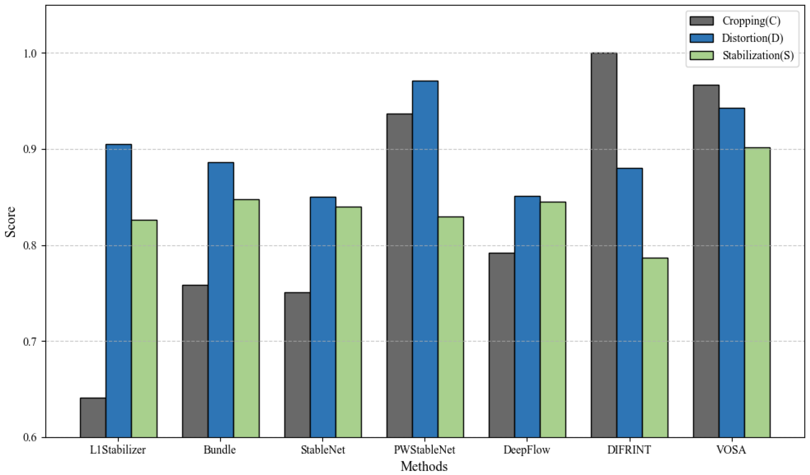
Specifically, the VOSA algorithm demonstrates significant advantages in both the cropping rate score and the distortion score, achieving high-quality video stabilization results. Unlike the other warping-based methods listed in Table 6 and Figure 8, DIFRINT [22] uses a technical path based on frame interpolation to achieve full-frame video stabilization. In terms of evaluation metrics, the algorithm does perform better in terms of cropping rate scores; however, in terms of stability and distortion scores, it is slightly inferior to warping-based stabilization algorithms such as Bundle [40] and PWStabNet.
In addition, it can be seen from the experimental data that the VOSA algorithm not only effectively reduces the scaling of video frames by reducing cropping but also mitigates the jitter amplification effect to a certain extent. The original intention of the cropping operation is to remove the holes around the boundaries of video frames due to missing pixels. However, in this process, it is often difficult to ensure that the aspect ratio of the original frame remains unchanged. Especially when the holes dominate at one of the frame boundaries, the cropped output may produce a large distortion due to the change in aspect ratio, which results in a lower distortion score. In contrast, the VOSA algorithm better preserves the aspect ratio of the initial frame by cleverly expanding the frame boundary by extrapolation, which effectively reduces the distortion level.
In addition, the VOSA algorithm, as a plug-and-play module with flexibility and versatility, when used in combination with various types of warping-based video stabilization algorithms, brings a significant enhancement to the algorithm’s rendering in terms of the evaluation index system. Specific data are shown in Table 7 and Figure 9.
From the experimental data in Table 7, it can be seen from the experimental data in Table 4 that VOSA comprehensively improves the warping-based video stabilization algorithms in terms of the CDS evaluation index system. Specifically, in terms of the cropping rate score, the method in this chapter improves StableNet [41] particularly significantly, with its score increasing from 0.754 to 0.874, and this substantial improvement fully demonstrates the effectiveness of the method in optimizing the cropping strategy in this chapter. As for the distortion score, after combining the algorithms in this chapter, PWStableNet [19] stands out and achieves the highest score, which further proves that the addition of VOSA reduces the distortion in the output video. On top of that, VOSA also achieved some degree of improvement in stability.
Visual Qualitative Analysis. In order to visually verify the actual effect of VOSA on vision, we use visual evaluation for experimental verification. In order to simplify the experimental comparison results, we only conduct experiments on the Video+Sensor [39] dataset to show the improvement of the algorithm in visual stabilization in a more focused way. As shown in Figure 10, more visual details can be included in the output stabilized frames by PWStabNet, DeepFlow, and VOSA processing. Through this series of visual evaluation experiments, we expect to be able to visualize the significant effectiveness of VOSA in improving video quality and reducing jitter and distortion.

5. Conclusions

Existing warping-based video stabilization algorithms smooth camera trajectories by constraining pixel displacements and warping unstable frames to stable frames. However, when searching unstable frames via transform matrices, insufficient pixels often cause missing regions in output frames. To solve this, we propose a boundary synthesis algorithm that leverages video motion’s inherent symmetry properties, particularly translational and rotational symmetry, to compensate for missing pixels using neighboring frame information.
Through the spatial coherence under symmetry constraints, VOSA extrapolates the view outside the boundary by aligning the neighboring frames with each reference frame. Technically, it first computes the optical flow and extends it to the outer boundary region of the view based on symmetry-aware affinity, thereby generating enough pixels for the subsequent warping process. The pixels are then warped accordingly. VOSA can be integrated as a plug-and-play module in a variety of methods to significantly reduce cropping in the steady image output results. And the stability of the algorithm is also improved to some extent due to the reduction in the jitter amplification effect caused by cropping and frame resizing.
Experimental results based on CDS evaluation metrics show that VOSA can improve the performance and visual effect of previously proposed algorithms in terms of objective metrics and subjective visual quality. This is of great significance for improving the video quality, enhancing the visual effect as well as improving the viewing experience of video users.
From the experimental results, it is evident that our proposed algorithm excels in stabilizing videos under a wide range of vibration conditions, including both low-frequency and high-frequency vibrations. The tests conducted demonstrate that the algorithm effectively compensates for camera displacement, reducing cropping artifacts and maintaining visual integrity.
However, while the method performs well in stable and moderately dynamic environments, it may underperform in highly dynamic scenes with irregular motion, where assumptions of rotational and translational symmetry are violated. This could lead to boundary artifacts that affect the quality of the stabilization. The symmetry-based optical flow extrapolation relies heavily on these assumptions, which may not hold in fast, erratic motions, such as those often encountered in extreme camera shakes or unpredictable scenes. At the same time, while the Video+Sensor dataset provides valuable sensor-augmented real-world sequences, its size is a limitation.
Future work will focus on three aspects: refining the symmetry adaptation mechanism to handle non-symmetric motion by incorporating scene complexity metrics; optimizing the network architecture to reduce computational costs without sacrificing performance, enabling broader deployment in resource-constrained scenarios; and expanding our validation to larger datasets that include both visual content and inertial sensor logs (e.g., extended sensor-augmented video collections) to further demonstrate the generalizability of our approach. This will allow us to verify VOSA’s performance across more diverse scenarios while maintaining the critical link between visual stabilization and hardware-specific motion data.

Supplementary Materials

The following supporting information can be downloaded at: https://storage.googleapis.com/dataset_release/all.zip accessed on 2 August 2025.

Author Contributions

Conceptualization, Y.W.; Methodology, X.L. and Y.W.; Software, Y.W.; Validation, Y.W.; Formal analysis, W.S. and H.Z.; Investigation, C.J.; Resources, C.J.; Data curation, C.J.; Writing—original draft, W.S. and Y.T.; Writing—review and editing, W.S., H.Z. and Z.C.; Visualization, Q.H.; Supervision, H.Z., Q.H., Z.C. and Y.T.; Project administration, H.Z., X.L., Z.C. and Y.T.; Funding acquisition, X.L. All authors have read and agreed to the published version of the manuscript.

Funding

This work was supported in part by the Opening Foundation of the Jiangsu Engineering Research Center of Digital Twinning Technology for Key Equipment in Petrochemical Process under grant numbers DTEC202303 and DTEC202301. This work was funded in part by the National Key Research and Development Program of China (Grant No. 2024YFC3210300). This work was funded in part by the National Natural Science Foundation of China (Grant No. 62401196), Natural Science Foundation of Jiangsu Province (Grant No. BK20241508), Fundamental Research Funds for the Central Universities (Grant No. B250201044).

Data Availability Statement

Supplementary Materials for this study, covering source code, datasets, and other related resources, are available upon request from the authors. In the future, these Supplementary Materials may be (partially or fully) published in online repositories such as GitHub, aiming to enhance the reproducibility of the study and facilitate in-depth exploration and academic exchange in related fields.

Conflicts of Interest

The authors declare that they have no known competing financial interests or personal relationships that could have appeared to influence the work reported in this paper.

References

  1. Zhang, L.; Xu, Q.K.; Huang, H. A Global Approach to Fast Video Stabilization. IEEE Trans. Circuits Syst. Video Technol. 2017, 27, 225–235. [Google Scholar] [CrossRef]
  2. Yan, W.; Sun, Y.; Zhou, W.; Liu, Z.; Cong, R. Deep Video Stabilization via Robust Homography Estimation. IEEE Signal Process. Lett. 2023, 30, 1602–1606. [Google Scholar] [CrossRef]
  3. Liu, S.; Zhang, Z.; Liu, Z.; Tan, P.; Zeng, B. Minimum Latency Deep Online Video Stabilization and Its Extensions. IEEE Trans. Pattern Anal. Mach. Intell. 2025, 47, 1238–1249. [Google Scholar] [CrossRef]
  4. Ren, Z.; Fang, M.; Chen, C.; Kaneko, S.i. Video stabilization algorithm based on virtual sphere model. J. Electron. Imaging 2021, 30, 021002. [Google Scholar] [CrossRef]
  5. Zhang, T.; Xia, Z.; Li, M.; Zheng, L. DIN-SLAM: Neural Radiance Field-Based SLAM with Depth Gradient and Sparse Optical Flow for Dynamic Interference Resistance. Electronics 2025, 14, 1632. [Google Scholar] [CrossRef]
  6. Norbelt, M.; Luo, X.; Sun, J.; Claude, U. UAV Localization in Urban Area Mobility Environment Based on Monocular VSLAM with Deep Learning. Drones 2025, 9, 171. [Google Scholar] [CrossRef]
  7. Huang, H.Y.; Huang, S.Y. Fast Hole Filling for View Synthesis in Free Viewpoint Video. Electronics 2020, 9, 906. [Google Scholar] [CrossRef]
  8. Liu, S.; Tan, P.; Yuan, L.; Sun, J.; Zeng, B. MeshFlow: Minimum Latency Online Video Stabilization. In Proceedings of the 2016 European Conference on Computer Vision, Amsterdam, The Netherlands, 11–14 October 2016; Springer: Cham, Switzerland, 2016; pp. 800–815. [Google Scholar]
  9. Grundmann, M.; Kwatra, V.; Essa, I. Auto-directed video stabilization with robust L1 optimal camera paths. In Proceedings of the CVPR 2011, Colorado Springs, CO, USA, 20–25 June 2011; pp. 225–232. [Google Scholar] [CrossRef]
  10. Bradley, A.; Klivington, J.; Triscari, J.; van der Merwe, R. Cinematic-L1 Video Stabilization with a Log-Homography Model. arXiv 2020, arXiv:cs.CV/2011.08144. [Google Scholar]
  11. Liu, S.; Yuan, L.; Tan, P.; Sun, J. SteadyFlow: Spatially Smooth Optical Flow for Video Stabilization. In Proceedings of the 2014 IEEE Conference on Computer Vision and Pattern Recognition, Columbus, OH, USA, 23–28 June 2014; pp. 4209–4216. [Google Scholar] [CrossRef]
  12. Zhang, L.; Chen, X.Q.; Kong, X.Y.; Huang, H. Geodesic Video Stabilization in Transformation Space. IEEE Trans. Image Process. 2017, 26, 2219–2229. [Google Scholar] [CrossRef]
  13. Wu, H.; Xiao, L.; Lian, Z.; Shim, H.J. Locally Low-Rank Regularized Video Stabilization With Motion Diversity Constraints. IEEE Trans. Circuits Syst. Video Technol. 2019, 29, 2873–2887. [Google Scholar] [CrossRef]
  14. Zhang, F.; Li, X.; Wang, T.; Zhang, G.; Hong, J.; Cheng, Q.; Dong, T. High-Precision Satellite Video Stabilization Method Based on ED-RANSAC Operator. Remote Sens. 2023, 15, 3036. [Google Scholar] [CrossRef]
  15. Jang, J.; Ban, Y.; Lee, K. Dual-Modality Cross-Interaction-Based Hybrid Full-Frame Video Stabilization. Appl. Sci. 2024, 14, 4290. [Google Scholar] [CrossRef]
  16. Li, X.; Xu, F.; Liu, F.; Tong, Y.; Lyu, X.; Zhou, J. Semantic Segmentation of Remote Sensing Images by Interactive Representation Refinement and Geometric Prior-Guided Inference. IEEE Trans. Geosci. Remote Sens. 2024, 62, 5400318. [Google Scholar] [CrossRef]
  17. Li, X.; Xu, F.; Yu, A.; Lyu, X.; Gao, H.; Zhou, J. A Frequency Decoupling Network for Semantic Segmentation of Remote Sensing Images. IEEE Trans. Geosci. Remote Sens. 2025, 63, 5607921. [Google Scholar] [CrossRef]
  18. Li, X.; Xu, F.; Zhang, J.; Yu, A.; Lyu, X.; Gao, H.; Zhou, J. Dual-domain decoupled fusion network for semantic segmentation of remote sensing images. Inf. Fusion 2025, 124, 103359. [Google Scholar] [CrossRef]
  19. Zhao, M.; Ling, Q. PWStableNet: Learning Pixel-Wise Warping Maps for Video Stabilization. IEEE Trans. Image Process. 2020, 29, 3582–3595. [Google Scholar] [CrossRef]
  20. Yu, J.; Ramamoorthi, R. Learning Video Stabilization Using Optical Flow. In Proceedings of the 2020 IEEE/CVF Conference on Computer Vision and Pattern Recognition (CVPR), Seattle, WA, USA, 13–19 June 2020; pp. 8156–8164. [Google Scholar] [CrossRef]
  21. Xu, Y.; Zhang, J.; Maybank, S.J.; Tao, D. DUT: Learning Video Stabilization by Simply Watching Unstable Videos. IEEE Trans. Image Process. 2022, 31, 4306–4320. [Google Scholar] [CrossRef]
  22. Choi, J.; Kweon, I.S. Deep Iterative Frame Interpolation for Full-frame Video Stabilization. ACM Trans. Graph. 2020, 39, 1–9. [Google Scholar] [CrossRef]
  23. Hartley, R.; Zisserman, A. Multiple View Geometry in Computer Vision, 2nd ed.; Cambridge University Press: Cambridge, UK, 2004. [Google Scholar]
  24. Wei, X.; Zhang, Y.; Li, Z.; Fu, Y.; Xue, X. DeepSFM: Structure from Motion via Deep Bundle Adjustment. In Proceedings of the Computer Vision—ECCV 2020: 16th European Conference, Glasgow, UK, 23–28 August 2020; Proceedings, Part I. Springer: Berlin/Heidelberg, Germany, 2020; pp. 230–247. [Google Scholar] [CrossRef]
  25. Kim, D.; Woo, S.; Lee, J.Y.; Kweon, I.S. Deep video inpainting. In Proceedings of the IEEE/CVF Conference on Computer Vision and Pattern Recognition, Long Beach, CA, USA, 15–20 June 2019; pp. 5792–5801. [Google Scholar]
  26. Li, J.; He, F.; Zhang, L.; Du, B.; Tao, D. Progressive Reconstruction of Visual Structure for Image Inpainting. In Proceedings of the IEEE/CVF International Conference on Computer Vision (ICCV), Seoul, Republic of Korea, 27 October–2 November October 2019. [Google Scholar]
  27. Zeng, Y.; Fu, J.; Chao, H. Learning Joint Spatial-Temporal Transformations for Video Inpainting. In Proceedings of the Computer Vision—ECCV 2020: 16th European Conference, Glasgow, UK, 23–28 August 2020; Proceedings, Part XVI. Springer: Berlin/Heidelberg, Germany, 2020; pp. 528–543. [Google Scholar] [CrossRef]
  28. Li, S.; He, F.; Du, B.; Zhang, L.; Xu, Y.; Tao, D. Fast Spatio-Temporal Residual Network for Video Super-Resolution. In Proceedings of the IEEE/CVF Conference on Computer Vision and Pattern Recognition (CVPR), Long Beach, CA, USA, 15–20 June 2019; pp. 10514–10523. [Google Scholar]
  29. Lim, B.; Son, S.; Kim, H.; Nah, S.; Lee, K.M. Enhanced Deep Residual Networks for Single Image Super-Resolution. In Proceedings of the 2017 IEEE Conference on Computer Vision and Pattern Recognition Workshops (CVPRW), Honolulu, HI, USA, 21–26 July 2017; pp. 1132–1140. [Google Scholar] [CrossRef]
  30. Zhang, Y.; Tian, Y.; Kong, Y.; Zhong, B.; Fu, Y. Residual Dense Network for Image Super-Resolution. In Proceedings of the 2018 IEEE/CVF Conference on Computer Vision and Pattern Recognition, Salt Lake City, UT, USA, 18–23 June 2018; pp. 2472–2481. [Google Scholar] [CrossRef]
  31. Lowe, D. Distinctive Image Features from Scale-Invariant Keypoints. Int. J. Comput. Vis. 2004, 60, 91–110. [Google Scholar] [CrossRef]
  32. Bay, H.; Tuytelaars, T.; Van Gool, L. SURF: Speeded up robust features. In Proceedings of the 9th European Conference on Computer Vision; Graz, Austria, 7–13 May 2006, Volume Part I; Springer: Berlin/Heidelberg, Germany, 2006; pp. 404–417. [Google Scholar] [CrossRef]
  33. Rublee, E.; Rabaud, V.; Konolige, K.; Bradski, G. ORB: An efficient alternative to SIFT or SURF. In Proceedings of the 2011 International Conference on Computer Vision, Barcelona, Spain, 6–13 November 2011; pp. 2564–2571. [Google Scholar] [CrossRef]
  34. DeTone, D.; Malisiewicz, T.; Rabinovich, A. Deep Image Homography Estimation. arXiv 2016. [Google Scholar] [CrossRef]
  35. Nguyen, T.; Chen, S.W.; Shivakumar, S.S.; Taylor, C.J.; Kumar, V. Unsupervised Deep Homography: A Fast and Robust Homography Estimation Model. IEEE Robot. Autom. Lett. 2018, 3, 2346–2353. [Google Scholar] [CrossRef]
  36. Zhang, J.; Wang, C.; Liu, S.; Jia, L.; Ye, N.; Wang, J.; Zhou, J.; Sun, J. Content-Aware Unsupervised Deep Homography Estimation. In Proceedings of the Computer Vision—ECCV 2020: 16th European Conference, Glasgow, UK, 23–28 August 2020; Proceedings, Part I. Springer: Berlin/Heidelberg, Germany, 2020; pp. 653–669. [Google Scholar] [CrossRef]
  37. Ilg, E.; Mayer, N.; Saikia, T.; Keuper, M.; Dosovitskiy, A.; Brox, T. FlowNet 2.0: Evolution of Optical Flow Estimation with Deep Networks. In Proceedings of the 2017 IEEE Conference on Computer Vision and Pattern Recognition (CVPR), Honolulu, HI, USA, 21–26 July 2017; pp. 1647–1655. [Google Scholar] [CrossRef]
  38. Brezinski, C.; Zaglia, M. Extrapolation Methods: Theory and Practice; Studies in Computational Mathematics; Elsevier: North Holland, The Netherlands, 2013. [Google Scholar]
  39. Shi, Z.; Shi, F.; Lai, W.S.; Liang, C.K.; Liang, Y. Deep Online Fused Video Stabilization. In Proceedings of the IEEE/CVF Winter Conference on Applications of Computer Vision, Waikoloa, HI, USA, 3–8 January 2022; pp. 1250–1258. [Google Scholar]
  40. Liu, S.; Yuan, L.; Tan, P.; Sun, J. Bundled camera paths for video stabilization. ACM Trans. Graph. 2013, 32, 1–10. [Google Scholar] [CrossRef]
  41. Wang, M.; Yang, G.Y.; Lin, J.K.; Zhang, S.H.; Shamir, A.; Lu, S.P.; Hu, S.M. Deep Online Video Stabilization With Multi-Grid Warping Transformation Learning. IEEE Trans. Image Process. 2019, 28, 2283–2292. [Google Scholar] [CrossRef] [PubMed]
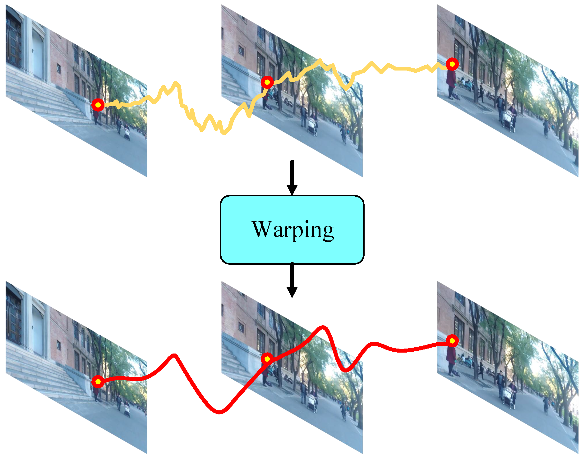
Figure 1. Schematic diagram of the warping process. The top row shows three consecutive frames from the original unstable video sequence, which are affected by camera shake and motion jitter. These frames are misaligned due to uncontrolled camera motion. The bottom row presents the corresponding warped frames that have been spatially transformed to align with a smoothed motion trajectory, resulting in a stabilized output.
Symmetry 17 01351 g001
Figure 2. The size of the frame output after warping is reduced, and the frame aspect ratio is changed. This figure illustrates how traditional warping-based stabilization methods reduce the output frame size and alter the original aspect ratio. To maintain visual consistency, cropped boundaries are often removed, leading to resolution loss and possible distortion. The visualization highlights how stabilized frames become smaller than the input, with black borders indicating missing content.
Symmetry 17 01351 g002
Figure 3. Video stabilization algorithm based on frame interpolation. This figure shows the principle of full-frame stabilization using intermediate frame interpolation. The top row displays the input video sequence, and the arrows represent the iterative interpolation steps. The output stabilized video at the bottom retains full-frame content by generating the missing pixels between the original frames.
Symmetry 17 01351 g003
Figure 4. Feature point matching and mismatch rejection. This figure shows the process of detecting and matching feature points between consecutive frames using SIFT, followed by RANSAC for outlier rejection. Yellow dots indicate detected keypoints, red dots represent correct matches, and purple dots denote rejected mismatches. This step ensures robust spatial alignment, which is critical for the pre-alignment module in the proposed stabilization framework.
Symmetry 17 01351 g004
Figure 5. Overview of VOSA. This figure presents the main pipeline of the View Out-boundary Synthesis Algorithm (VOSA). The process starts with pre-alignment of frame sequences, followed by optical flow estimation using FlowNet2. Affinity propagation is then applied to guide warping and boundary extrapolation. The output is a stabilized video sequence with expanded view boundaries and reduced cropping.
Symmetry 17 01351 g005
Figure 6. Frame boundary processing. This figure illustrates how the optical flow field is extended beyond the visible area using affinity kernels. The shared view region between the current frame and a pre-aligned reference frame is used to estimate motion. Motion propagation enables extrapolation to missing regions, supporting full-frame reconstruction.
Symmetry 17 01351 g006
Figure 7. Codec network schematic. This figure shows the codec-style network used to predict the affinity kernel and refined optical flow. The encoder processes input frames, masks, and Sobel-edge maps, while the decoder fuses multi-scale features to output the refined optical flow and affinity kernels.
Symmetry 17 01351 g007
Figure 8. Performance comparison of VOSA with other methods.
Symmetry 17 01351 g008
Figure 9. VOSA performance enhancements to existing methods.
Symmetry 17 01351 g009
Figure 10. Visual qualitative analysis of PWStabNet, DeepFlow, and VOSA. This figure compares original unstable frames with stabilized frames produced by PWStabNet, DeepFlow, and VOSA. The left column shows the input with visible jitter and missing content near the boundaries. The right column presents the output with enhanced frame completeness and reduced distortion. More scene content is retained without cropping, confirming the effectiveness of the proposed boundary synthesis approach.
Symmetry 17 01351 g010
Table 1. Hyperparameters of the VOSA model.
CategoryHyperparameterValue
OptimizationOptimizerAdam
Adam beta parameters(0.9, 0.99)
Momentum coefficient0.9
Weight decay (initial)2 × 10⁻⁴
Boundary ProcessingBoundary padding80 pixels per side
Iteration count for propagation10
SIFTContrast threshold0.04
Edge threshold10
Octaves4
RANSACDistance threshold5 pixels
Inlier ratio threshold0.8
Network DesignSobel filter size3 × 3
Affinity kernel radius r = 4
Table 2. The detailed network configuration of our encoder.
LayerKernelStrides
Conv1 3 × 3 1
Conv2 3 × 3 1
MaxPool2 4 × 4 4
Conv3 3 × 3 1
MaxPool3 4 × 4 4
Conv4 3 × 3 1
MaxPool4 4 × 4 4
Conv5 3 × 3 1
MaxPool5 4 × 4 4
Table 3. Comparative analysis of pre-aligned modules.
ModelCDS
Baseline0.9100.9490.900
w/o Pre-Alignment Module0.9400.9260.900
w Pre-Alignment Module0.9670.9430.902
Table 4. Comparison of results for the corresponding parameters of the loss function.
Loss ParameterCDS
α = 2 , β = 0 0.9240.9520.900
α = 2 , β = 1.5 0.9450.9400.902
α = 2 , β = 2.5 0.9470.9430.900
α = 1.5 , β = 2 0.9650.9440.900
α = 2.5 , β = 2 0.9670.9420.902
α = 2 , β = 2 0.9670.9430.902
Table 5. Iteration count performance comparison.
Number of IterationsCDS
00.9100.9490.900
50.9470.9510.900
100.9670.9430.902
150.9670.9310.902
200.9700.9150.902
Table 6. Performance comparison of VOSA with other methods on Video+Sensor [39] dataset.
MethodsCDS
L1Stabilizer [9]0.6410.9050.826
Bundle [40]0.7580.8860.848
StableNet [41]0.7510.8500.840
PWStableNet [19]0.9370.9710.830
DeepFlow [20]0.7920.8510.845
DIFRINT [22]1.0000.8800.787
VOSA0.9670.9430.902
Table 7. Performance enhancement of VOSA over other warping-based image stabilization methods.
MethodsCDS
MeshFlow [8]0.7700.6780.813
MeshFlow+VOSA0.8980.6830.823
StableNet [41]0.7540.8510.843
StableNet+VOSA0.8470.8970.850
PWStableNet [19]0.9310.9690.832
PWStableNet+VOSA0.9470.9730.843
Disclaimer/Publisher’s Note: The statements, opinions and data contained in all publications are solely those of the individual author(s) and contributor(s) and not of MDPI and/or the editor(s). MDPI and/or the editor(s) disclaim responsibility for any injury to people or property resulting from any ideas, methods, instructions or products referred to in the content.