Symmetry-Enhanced Locally Adaptive COA-ELM for Short-Term Load Forecasting

Abstract

Reliable short-term electricity usage prediction is essential for preserving the stability of topologically symmetric power networks and their dynamic supply–demand equilibrium. To tackle this challenge, this paper proposes a novel approach derived from the standard Extreme Learning Machine (ELM) by integrating an enhanced Crayfish Optimization Algorithm (DSYCOA). This algorithm combines Logistic chaotic mapping, local precise search, and dynamic parameter adjustment strategies designed to achieve a dynamic balance between exploration and exploitation, thereby optimizing the initial thresholds and weights of the ELM. Consequently, a new short-term power load forecasting model, namely the DSYCOA-ELM model, is developed. Experimental validation demonstrates that the improved DSYCOA exhibits fast convergence speed and high convergence accuracy, and successfully harmonizes global exploration and local exploitation capabilities while maintaining an empirical balance between exploration and exploitation. To additionally verify the effectiveness of DSYCOA in improving ELM, this paper conducts simulation comparison experiments among six models, including DSYCOA-ELM, ELM, and ELM improved by BWO (BWO-ELM). The findings demonstrate that the DSYCOA-ELM model outperforms the other five forecasting models in terms of Mean Absolute Percentage Error (MAPE), Mean Absolute Error (MAE), Root Mean Squared Error (RMSE), and other indicators. Specifically, in terms of MAPE, DSYCOA-ELM reduces the error by 96.9% compared to ELM. This model demonstrates feasibility and effectiveness in solving the problem of short-term power load prediction, providing critical support for maintaining the stability of grid topological symmetry and supply–demand balance.

1. Introduction

Accurate short-term electricity demand prediction serves as a vital basis for the operation and planning of power systems. The accuracy of this forecasting directly impacts the safe, stable, and economic functioning of power systems. Precise short-term load forecasting can assist power departments in reasonably arranging generation plans, optimizing resource allocation, and reducing operational costs [1], which is highly important for enhancing the operational efficiency and reliability of power systems. Lately, with the continuous expansion of electricity grid scales and the deepening advancement of power market reforms, electric load characteristics have become increasingly complex. Conventional approaches to load forecasting have struggled to match the prediction accuracy requirements of modern power systems. Therefore, researching high-precision, high-efficiency short-term electric load forecasting methods holds significant theoretical and practical value.

Existing short-term electrical load forecasting methods are mainly categorized into three types: traditional statistical model-based, machine learning-based, and hybrid model-based. Traditional statistical model-based methods build models on prior knowledge and statistical assumptions, simplifying complexity for stable forecasts. Typical examples are the Grey Model (GM) [2], which is a first-order, one-variable model used for forecasting; the Autoregressive Integrated Moving Average (ARIMA) [3], a statistical model for time series forecasting; and time series analysis models [4]. These methods have the advantages of low data demand and strong robustness. However, their prediction performance is limited by inherent assumptions and they are highly sensitive to data features. To overcome these limitations, researchers have proposed various model improvement strategies. For example, Wu F et al. enhanced the traditional ARIMA model through optimization with the Cuckoo Search (CS) algorithm, significantly improving its forecasting accuracy [5]. Yuhong W et al. enhanced the classic gray (1, 1) model’s prediction precision by dynamically optimizing the background value and initial conditions utilizing the Mean Value Theorem (MVT) and minimizing the relative error criterion [6]. Yet, traditional statistical methods have inherent flaws such as limited scenario adaptability, insufficient nonlinear modeling ability, and weak high-dimensional data processing capacity.

Against this backdrop, AI technologies like traditional machine learning [7,8,9,10,11,12] and deep learning [13,14,15,16] have been introduced to offer innovative solutions. For instance, Singh S.N. et al. developed a load forecasting model combining wavelet transform (WT) and support vector machine (SVM), accurately forecasting power loads using historical time series data [17]. Fan G F et al. created a new short-term electrical power load estimation model integrating the random forest (RF) and mean generating function (MGF) models, greatly improving the original model’s prediction accuracy [12]. Relative to standard machine learning algorithms, deep learning algorithms can extract more elaborate and advanced representations from the raw data, thus enhancing the precision of prediction results. For example, Yuqi, J. et al. [18] proposed a new feature set and input them into the LSTM neural network for prediction. Lin J. et al. [16] proposed a dual-step attention-focused LSTM network for short-term zonal load probabilistic forecasting, which showed greater accuracy and stronger generalization ability than other cutting-edge models. However, machine-learning-based prediction methods generally have the risk of overfitting, and their performance heavily depends on large-scale high-quality training data, which may be hard to obtain in practical electrical load forecasting scenarios. To integrate the advantages of different methods and build a forecasting framework with complementary features, hybrid model approaches have become a research hotspot. Li K. et al. [14] presented a hybrid electrical load prediction model integrating CEEMDAN-SE and LSTM. Nie Y. et al. [19] formulated an innovative hybrid model for electrical load prediction integrating data preparation techniques, individual forecasting algorithms, and weight assignment theory. Hybrid models, by combining the interpretability of traditional methods with the high noise-tolerance ability of machine learning, address the challenges faced by single models.

However, hybrid models often encounter issues like structural complexity, long training times, and high computational resource consumption in practical applications. In this context, the Extreme Learning Machine [20] (ELM), an emerging machine learning algorithm, has gained increasing attention. ELM is a high-speed learning algorithm for single-hidden-layer feedforward neural networks (SLFNs). Its core idea is to randomly generate the hidden layer parameters and directly calculate the output weights using the least squares method. Compared with the aforementioned methods, ELM offers advantages including high computational efficiency, strong generalization ability, and good model interpretability, and has yielded outstanding outcomes in numerous practical applications [21,22,23,24]. Nevertheless, the random initialization of input weights in ELM, while enhancing training speed and generalization ability to some extent, also presents the main bottleneck to its performance improvement. The randomness implies that each initialization may yield a different model, a problem that becomes particularly pronounced when dealing with complex or high-dimensional data. High-dimensional data often contain rich information and complex structures, and randomly generated weights may fail to adequately capture these intrinsic patterns and characteristics, leading to less-than-satisfactory model performance in prediction tasks. To address this issue, researchers have attempted to improve ELM using various optimization algorithms [25,26,27,28,29], which have effectively enhanced the model’s prediction accuracy and stability. However, when addressing intricate optimization challenges, these algorithms still face issues such as low search efficiency and a propensity to converge on local optima.

To address the limitations of existing methods, this paper proposes a novel short-term load forecasting model that integrates an enhanced Crayfish Optimization Algorithm (DSYCOA) with the Extreme Learning Machine (ELM). The traditional Crayfish Optimization Algorithm, while effective in certain contexts, has limitations such as susceptibility to local optima and suboptimal convergence rates. To overcome these limitations, this paper introduces several improvements to the Crayfish Optimization Algorithm, including Logistic chaotic mapping to enhance population diversity, local precise search to refine solutions, and dynamic parameter adjustment to balance exploration and exploitation. These enhancements significantly boost the algorithm’s global exploration capability and convergence rate. The improved algorithm is then utilized to optimize the initial weights and biases of the ELM, resulting in the DSYCOA-ELM forecasting model. This model not only improves the prediction accuracy and convergence speed but also demonstrates robustness against outliers and noisy data, making it highly suitable for real-time applications in modern power systems.

2. The ELM Model

ELM is a training algorithm for feedforward neural networks, and its structure mainly consists of three layers: the input layer, the hidden layer, and the output layer. The input layer is responsible for receiving raw data, typically without involving any computation or transformation, directly passing the data to the hidden layer. The hidden layer comprises multiple neurons, tasked with feature extraction from the data. The hidden layer’s output values are subsequently transmitted to the output layer, which calculates the final prediction results based on the hidden layer’s output. As shown in Figure 1, the schematic diagram of the ELM structure is presented.

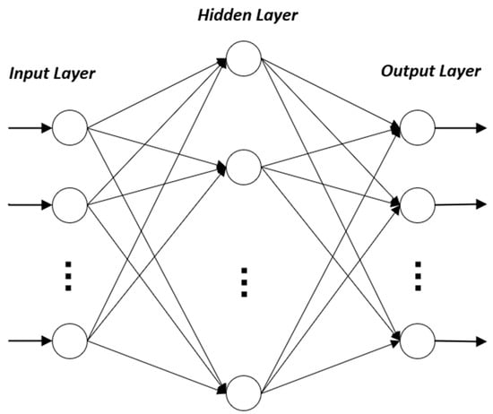
Figure 1. Illustration of ELM architecture.

Under the ELM framework, for any given input sample, the activation values for the hidden layer are calculated first, based on a set of input weights and bias parameters that are randomly initialized beforehand, combined with a specific activation function. Subsequently, efforts are made to accurately map the hidden layer’s output to the desired target output, the weights of the output layer are determined by solving an optimization problem, which is designed to minimize the prediction error between the model output and the actual observed values. The specific derivation process of ELM is as follows.

Assuming a given training set, where R denotes the real number field, $x_i$ represents the i-th data instance, which is a u-dimensional vector, i.e., the feature input vector; $l_i$ denotes the data label corresponding to the i-th data instance, which is a v-dimensional vector; and M represents the number of training samples. Let h_nb denote the number of hidden layer nodes in the ELM, and H(x) denote the output of the hidden layer. Then, the calculation formula for H(x) is given by Equation (1) as shown below.

$$H\left(x\right)=\left[h_1\right(x),h_2(x),\dots ,h_{h\_nb}(x\left)\right]$$

(1)

In the equation, $h_i\left(x\right)$ represents the output of the i-th hidden layer node. The hidden layer’s output is derived by multiplying the input vector by the weight vector corresponding to that node, adding a bias term, and then processing the result through a nonlinear activation function. $H\left(x\right)=\left[h_1\right(x),h_2(x),\dots ,h_{h\_nb}(x\left)\right]$ represents the nonlinear mapping of ELM. The output functions for hidden layer nodes are not uniform, and different hidden neurons can utilize different output functions. Generally, the definition of $h_i\left(x\right)$ is given by Equation (2) as shown below.

$$h_i\left(x\right)=g\left(w_i{,t}_i,x\right)=g\left(w_{i}x+t_i\right), w_i\in R^u,t_i\in R$$

(2)

where $w_i$ is a weight vector, representing the input weights of the i-th node in the hidden layer, $t_i$ is the bias term, and $g(·)$ denotes the activation function. The activation function is a nonlinear function used to introduce nonlinear characteristics, enabling the neural network to learn and simulate more complex functional mapping relationships. Since all load samples are non-negative, the strictly positive range (0, 1) of the sigmoid function is sufficient and avoids the extra mapping required by tanh, in this paper, the Sigmoid function, i.e., $g(x)={\displaystyle \frac{e^x}{1+e^{-x}}}$, is adopted to offer an in-depth explanation of training a single-hidden-layer feedforward neural network with ELM.

Let $\mathsf{\beta }={[{\mathsf{\beta }}_1,{\mathsf{\beta }}_2,\dots {\mathsf{\beta }}_{\mathrm{h}\_\mathrm{n}\mathrm{b}}]}^{\mathrm{T}}$ represent the output weights between the hidden layer and the output layer, then the output of the ELM is as shown in Equation (3).

$$f_{h\_nb}(x)={\sum }_{i=1}^{h\_nb}{\beta }_i{h}_i\left(x\right)=H\left(x\right)\beta$$

(3)

Throughout the training of SLFNs using ELM, the process is typically divided into two phases: random feature mapping and linear parameter optimization. In the feature mapping phase, the hidden layer’s weights and biases are initialized randomly, and the input data is projected into a new feature space using a nonlinear activation function. Notably, the parameters of the hidden layer nodes are generated randomly from a specific probability distribution, not through iterative training. This approach offers ELM a significant computational efficiency advantage over conventional backpropagation neural networks.

In the linear parameter solving phase, to obtain β that performs well on the training dataset and ensures the training error is minimized, the model uses the method of minimizing the sum of squared differences to solve for the weights β connecting the hidden layer and the output layer. The objective function is given by Equation (4). In the equation, H represents the output matrix of the hidden layer; C denotes the target matrix of the training data, as shown in Equations (5) and (6).

$$min{\left|\right|H\beta -C\left|\right|}^2, \beta ϵR^{h\_nb\times v}$$

(4)

$$H={\left[h\left(x_1\right),h\left(x_2\right),\dots h\left(x_M\right)\right]}^T$$

(5)

$$C=\left[\begin{array}{c}{c_1}^T\\ \begin{array}{c}⋮\\ {c_M}^T\end{array}\end{array}\right]$$

(6)

The optimal solution for the objective function in Equation (4) is calculated as shown in Equations (7) and (8).

$${\beta }^{*}=H^{†}B$$

(7)

$$H^{†}={\left(H^{T}H\right)}^{-1}{H}^T$$

(8)

where $H^{†}$ denotes the Moore–Penrose generalized inverse of matrix H.

3. Local Adaptive Parameter Adjustment COA

3.1. COA

COA is a novel heuristic optimization method that derives ideas from the natural performances of crayfish during the summer season, competition, and foraging phases. The algorithm is divided into three stages: summer avoidance, competition, and foraging, each of which draws inspiration from the corresponding behaviors of crayfish in nature. To elaborate, the phase of summer evasion in the algorithm acts as the exploration segment, whereas the stages of rivalry and searching symbolize the exploitation segments. The COA’s ability to explore and exploit is managed by a temperature parameter, which is subject to randomness. At high temperatures, crayfish tend to find shelter in burrows; if there is no contest for the burrow from other crayfish, they will enter it directly, indicating the start of the summer evasion phase of the COA. If competition for the burrow arises among other crayfish, this initiates the competitive phase of the COA. During suitable temperatures, crayfish do not seek shelter, leading the COA into the foraging phase. The COA effectively balances exploration and exploitation through temperature control, showcasing impressive optimization capabilities.

Assuming N is the number of individuals in the population and D is the size of the search space, the vector $X=[X_{i1},X_{i2},\dots ,X_{ij}]$ for i = 1, 2,…, N and j = 1, 2,…, D represents the position of crayfish i in the search space. ub and lb denote the maximum and minimum limits of the search space, respectively, with ${ub}_j$ and ${lb}_j$ specifically representing the upper and lower bounds for the j-th dimension. r is a random number between 0 and 1. The initialization phase of the COA is shown in Equation (9).

$$X_{ij}={lb}_j+({ub}_j-{lb}_j)\times r$$

(9)

Crayfish behavior is influenced by temperature fluctuations. When temperatures rise above 30 °C, crayfish retreat into burrows to escape the heat. Conversely, at more moderate temperatures, crayfish become active in foraging. The amount of foraging activity is also temperature-dependent. Within the range of 15 °C to 30 °C, crayfish are active in foraging, with 25 °C being the most favorable temperature, leading to a foraging quantity that follows a normal distribution. Assuming Temp indicates the ambient temperature in which crayfish reside, q represents the foraging quantity of crayfish, and μ represents the peak temperature for suitability for crayfish, with σ and $A_1$ controlling the intake quantity of crayfish at different temperatures. The environmental temperature and foraging quantity of crayfish are shown in Equations (10) and (11), respectively.

$$Temp=r\times 15+20$$

(10)

$$q=A_1\times 1/\sqrt{2\times \pi \times \sigma }\times exp(-{(t-\mu )}^2/2{\sigma }^2)$$

(11)

Assuming $X_{dx}$ represents the location of the cave, $X_{last}$ indicates the most advantageous position of the swarm post-prior revision, MT signifies the cap on iterations for the algorithm, and t is the current iteration count. The iteration formulas for the cave definition, summer avoidance phase, and competition phase are given in Equations (12)–(14), respectively.

$$X_{dx}=(X_{last}+X_{best})/2$$

(12)

$$X_{i,j}^{t+1}=X_{i,j}^t+A_2\times r\times (X_{dx}-X_{i,j}^t) r<0.5$$

(13)

$$X_{i,j}^{t+1}=X_{i,j}^t-X_{m,j}^t+X_{dx} r\ge 0.5$$

(14)

where ${\mathrm{A}}_2$ is a control coefficient, whose definition is given in Equation (15). Additionally, m represents a randomly selected crayfish individual, whose definition is provided in Equation (16).

$$A_2=2-(t/MT)$$

(15)

$$m=round(r\times (N-1\left)\right)+1$$

(16)

During the foraging phase, crayfish will determine whether to break down food based on its size. Let $X_f$ denote the food, with F representing the size of the food. Furthermore, let $f\left(i\right)$ represent the fitness value of the i-th crayfish, and $f\left(food\right)$ represent the fitness value at the location of the food. The definitions of $X_f$ and F are given in Equations (17) and (18), respectively.

$$X_f={\mathrm{X}}_{\mathrm{b}\mathrm{e}\mathrm{s}\mathrm{t}}$$

(17)

$$F=A_3\times r\times \left(f\right(i)/f(food\left)\right)$$

(18)

Here, $A_3$ denotes the food factor, with the constant 3 indicating the maximum amount of food available.

When $F>(A_3+1)/2$ is satisfied, if the food is too large for crayfish to consume directly, they must first tear the food into smaller pieces before foraging. The formulas for tearing food and iterating positions are shown in Equations (19) and (20), respectively. When the condition $F\le (A_3+1)/2$ is met, crayfish will forage directly. At this juncture, the iteration formula for crayfish position is given as in Equation (21).

$$X_f=exp(-1/F)\times X_f$$

(19)

$$X_{i,j}^{t+1}=X_{i,j}^t+X_f\times q\times \left(cos\right(2\times \pi \times r\left)\right)$$

(20)

$$X_{i,j}^{t+1}=(X_{i,j}^t-X_f)\times q+q\times r\times X_{i,j}^t$$

(21)

3.2. Locally Adaptive Parameter Tuning for the COA

To deal with the challenge of the COA being susceptible to local optima, this paper introduces three strategies: Logistic chaotic mapping, local precise search, and dynamic parameter adjustment. These strategies are employed to optimize and adjust the population before and during iterations, seeking to maintain equilibrium between the algorithm’s exploration and exploitation capabilities. By doing so, the algorithm’s global search capability is enhanced.

3.2.1. Logistic Chaotic Mapping Strategy

The Logistic chaotic mapping is a well-known chaotic system model initially proposed by Belgian mathematician Pierre François Verhulst in 1838. The core idea behind introducing this strategy is to utilize the chaotic characteristics exhibited by the Logistic mapping within a certain parameter range to generate the initial population for the algorithm. The ergodicity of chaotic systems and their sensitive dependence on initial conditions ensure that the generated random numbers broadly cover the entire search space, enhancing the randomness and diversity of the COA. This prevents the algorithm from being trapped in local optima and enhances its exploration capabilities and convergence efficiency.

The general form of the Logistic chaotic mapping is given in Equation (22).

$$x_{n+1}=R·x_n·(1-x_n)$$

(22)

Here, R is the control parameter of the logistic map, set to 3.99 in this paper to ensure chaotic behavior, while ${\mathrm{x}}_{\mathrm{n}}$ is initialized as a random value between 0 and 1.

A population of 30 individuals is generated within the two-dimensional range [−5, 5]. The Logistic chaotic mapping uses a control parameter of 3.99, the Tent chaotic mapping uses a breakpoint of 0.5, the Sine chaotic mapping uses a scaling factor of 4, and the Random initialization draws samples uniformly across the same bounds, as shown in Figure 2.

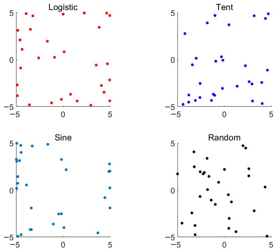
Figure 2. Comparison of four population generation methods.

According to Figure 2, the Logistic chaotic mapping method achieves the most uniform distribution of individuals across the entire search space. This uniformity enables the algorithm to explore a broader solution space from the outset, thereby reducing the risk of premature convergence to local optima. In contrast, while Random initialization also covers most of the search space, its distribution is less uniform compared to the Logistic method. The Tent and Sine mappings exhibit intermediate characteristics, with Tent showing slightly better coverage than Sine but still falling short of the Logistic method’s uniformity.

3.2.2. Local Precision Search Strategy

In the course of the iterative process of the COA, to effectively assist the algorithm in escaping local optima, this paper introduces a local precision search strategy. When condition $t>o.5\times MT$ is met, the algorithm evaluates the relationship between the global best fitness value and the currently found best fitness value. If the gap between the global best fitness value and the currently identified best fitness value is smaller than a specified threshold, the algorithm triggers a local search process. The core idea of this search process is to iteratively search within the vicinity of the current best position in an attempt to find a better solution. Specifically, in every iteration, the algorithm produces a new candidate solution and calculates its fitness value using the objective function. If the fitness value of the new solution surpasses the current best fitness value, both the best fitness value and the best position are updated. This process continues until the algorithm reaches the predetermined number of iterations or finds a better solution. Assuming the pre-determined threshold is denoted as search_ts, and the pre-determined number of iterations as search_nb, the generated candidate solutions are represented by C_X, and the fitness values of the candidate solutions are denoted by $f_{C\_X}$. Q is a D-dimensional random vector, whose elements are uniformly distributed in the interval [0, 1] and are independent of each other. The step size for local search is a constant, denoted as step_size. Considering both the search duration and precision of the algorithm, this paper sets step_size to 0.1. The detailed procedure of the local precise search strategy is described below:

• Step 1: Initialize the best fitness value $f_{best}={f(X}_{best})$ and the optimal position $X_{best}$.
• Step 2: For each iteration i = 1, 2, 3,…, search_nb:

• Generate a candidate solution according to Equation (23).

  $$C\_X=X_{best}+step\_size(Q\times 2-1)$$

  (23)
• Apply boundary conditions to ensure $C\_X$ stays within the search space, as shown in Equation (24).

  $$\mathrm{C}\_\mathrm{X}=\mathrm{m}\mathrm{a}\mathrm{x}\{\mathrm{l}\mathrm{b},\mathrm{m}\mathrm{i}\mathrm{n}(\mathrm{u}\mathrm{b},\mathrm{C}\_\mathrm{X}\left)\right\}$$

  (24)
• Calculate the fitness value of the candidate solution according to Equation (25).

  $$f_{C\_X}=f(C\_X)$$

  (25)
• If $f_{C\_X}<f_{best}$, then update the best fitness value and the optimal position according to Equations (26) and (27).

  $$f_{best}=f_{C\_X}$$

  (26)

  $$X_{best}=C\_X$$

  (27)

• Step 3: Return the best fitness value $f_{best}$ and the optimal position $X_{best}$.

Introducing this local precision search strategy helps the algorithm further refine the search results based on the global search, improving the algorithm’s accuracy and thus enhancing its global search capability and convergence efficiency.

3.2.3. Dynamic Parameter Adjustment Strategies

The locally precise search strategy introduced in this paper encompasses two parameters: the number of local iterations (search_nb) and the local search threshold (search_ts). The number of local iterations dictates how many attempts are made to seek a better solution during the local search process, while the local search threshold dictates when to trigger the local search to enhance the solution’s accuracy. The values of these two parameters directly impact the search efficiency and solution quality of the algorithm. If the number of iterations is set too low, the algorithm may fail to adequately explore the solution space, potentially leading to a premature convergence to a local optimum instead of the global optimum. Conversely, excessive iterations can result in inefficient use of computational resources and increase the algorithm’s runtime, especially in cases where the solution space is large or the problem complexity is high. Additionally, an improperly set local search threshold can also influence the algorithm’s efficiency and effectiveness. A threshold set too high may cause the algorithm to prematurely enter the local search phase, thereby neglecting a broader exploration of the solution space. Conversely, a threshold set too low may result in the algorithm expending excessive iterations in the local search phase, which may also result in inefficient use of computational resources.

Thus, to achieve a balance between the global and local search capabilities of the algorithm, this paper introduces a dynamic parameter adjustment strategy based on the local precise search strategy. The parameters search_nb and search_ts are dynamically adjusted during the algorithm’s iteration process. Specifically, search_ts decreases gradually according to a decay rate. Meanwhile, search_ts increases by 10 every iter_in_rate generations, where iter_in_rate is a constant representing the iteration increase rate. In this paper, the value of iter_in_rate is set to 5, and the threshold decay rate is set to 0.001.

Assuming that search_nb_initial denotes the initial value of the local iteration number, ts_de_rate represents the threshold decay rate, the dynamic adjustment formulas for search_nb and search_ts are shown in Equations (28) and (29), respectively.

$$search\_\mathrm{n}\mathrm{b}\left(t\right)=search\_\mathrm{n}\mathrm{b}\_initial+⌊t/iter\_in\_rate⌋\times ∆iter$$

(28)

$$search\_ts\left(t\right)=search\_ts(t-1)\times (1-ts\_de\_rate)$$

(29)

Through dynamic adjustment, the algorithm is capable of autonomously balancing exploration and exploitation based on feedback information during the search process (The term ‘balance’ is used here in an empirical sense rather than implying a rigorously defined symmetry metric). This enhances the algorithm’s precision by refining search results based on global search capabilities and enhancing convergence efficiency.

The pseudocode for the improved Crayfish Optimization Algorithm (COA), termed DSYCOA, is illustrated in Algorithm 1.

Algorithm 1: Pseudocode of DSYCOA

Input: N: Population size, MT: Maximum number of iterations, D: Dimension

Output: ${\mathrm{f}}_{\mathrm{b}\mathrm{e}\mathrm{s}\mathrm{t}}$: Optimal solution’s objective function value ${\mathrm{X}}_{\mathrm{b}\mathrm{e}\mathrm{s}\mathrm{t}}$: Optimal solution’s position

Algorithm Description:

1: Initializing the population using Logistic chaotic mapping

2: While t < 1/2MT

3:  Defining temperature Temp by Equation (10)

4:  If Temp >30

5:   Define cave $X_{dx}$ according to Equation (12)

6:    If r < 0.5

7:     Crayfish conducts the summer resort stage by Equation (13)

8:   Else

9:     Crayfish compete for caves by Equation (14)

10:   End

11:  Else

12:   The food intake $X_f$ and food size F are obtained through Equations (17) and (18)

13:   If F > 2

14:     Crayfish shreds food by Equation (19)

15:     Crayfish foraging according to Equation (20)

16:   Else

17:     Crayfish foraging according to Equation (21)

18:   End

19:  End

20:  Update fitness values $X_{best}, X_{last}$

21:  t = t + 1

22: End

23: While (t > 1/2MT)&&(t < MT)

24:  Repeat steps 3–18

25:  If ($f_{best}$ − $f_{last}$)/$f_{best}$ < search_ts

26:  Update search_nb according to Equation (28)

27:  Update search_ts according to Equation (29)

28:   Generate a candidate solution Equation (23)

29:   Ensure that according to Equation (24), the search remains within the search space

30:   Update the best fitness value and the best position according to Equations (26) and (27)

31:   t = t + 1

32:  Else

33:   Update fitness values $X_{best},X_{last}$ like step 20

34:   t = t + 1

35:  End

36: End

The flowchart of DSYCOA-ELM is shown in Figure 3.

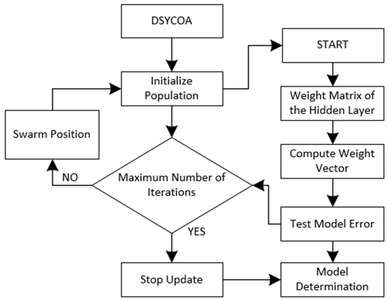
Figure 3. Convergence curves of DSYCOA-ELM.

If the maximum iteration count is reached before the error falls below 1 × 10⁻³, a secondary local refinement (Equations (23)–(27)) with an additional 5% iteration budget is automatically triggered. Across 100 independent runs this occurred in only two cases, and the final MAPE still remained below the threshold, confirming that the algorithm never terminates with persistently high error and that overall efficiency is preserved.

Figure 3 depicts the complete training pipeline of DSYCOA-ELM: the initial population is first created via Logistic chaotic mapping, with each individual encoding a set of ELM input weights and biases; the DSYCOA then drives global exploration and exploitation by simulating crayfish behaviors—summer avoidance, competition, or foraging—according to temperature, and applies a local precision search in the neighborhood of the global best after half the iterations if the threshold is met, while adaptively adjusting the local-search budget and trigger threshold; for every candidate, the hidden-layer output matrix is computed with the fixed weights and biases and the output weights are obtained in one step using the Moore–Penrose pseudoinverse; MAPE or MAE on the validation set serves as the fitness function, the historically best solution is retained and updated, and when the maximum iteration count is reached the globally optimal weights and biases are exported to form the final forecasting model, thereby improving both convergence speed and prediction accuracy while maintaining robustness.

3.3. Performance Validation of the DSYCOA

To demonstrate the superiority of the DSYCOA proposed in this paper, 21 benchmark test functions were selected and experiments were conducted on the Matlab R2020a platform (This 21 benchmark test functions—all taken from the IEEE CEC competition suite, which includes unimodal, multimodal, hybrid, and composite types and is widely recognized as an authoritative benchmark for assessing modern optimization algorithms). The basic information of these 21 benchmark test functions is presented in Table 1. Specifically, $F_1$ represents a unimodal function, primarily utilized to evaluate the convergence speed and accuracy of the algorithm. Functions $F_2~F_7$ are simple multimodal functions, aimed at evaluating the algorithm’s capability to avoid local optima. Functions $F_8~F_{14}$ constitute mixed functions, while functions $F_{15}~F_{21}$ are composite functions. Both of these function types are characterized by high complexity and difficulty in solving, acting as essential benchmarks to evaluate how well the algorithm balances global search and local search capabilities.

Table 1. Information on benchmark test functions.

Type	No.	Description	${{\mathit{F}}_{\mathit{i}}}^{\mathit{*}}$
Unimodal functions	1	Shifted and Roatated Bent Cigar Function	100
Simple Multimodal functions	2	Shifted and Rotated Rastrigin’s Function	500
	3	Shifted and Rotated Expanded Scaffer’s F6 Function	600
	4	Shifted and Rotated Lunacek Bi-Rastrigin Function	700
	5	Shifted and Rotated Non-Continuous Rastrigin’s Function	800
	6	Shifted and Rotated Levy Function	900
	7	Shifted and Rotated Schwefel’s Function	1000
Hybrid functions	8	Hybrid Function 2 (N = 3)	1200
	9	Hybrid Function 3 (N = 3)	1300
	10	Hybrid Function 5 (N = 4)	1500
	11	Hybrid Function 6 (N = 4)	1600
	12	Hybrid Function 6 (N = 5)	1800
	13	Hybrid Function 6 (N = 5)	1900
	14	Hybrid Function 6 (N = 6)	2000
Composition Functions	15	Composition Function 1 (N = 3)	2100
	16	Composition Function 2 (N = 3)	2200
	17	Composition Function 6 (N = 5)	2600
	18	Composition Function 7 (N = 6)	2700
	19	Composition Function 8 (N = 6)	2800
	20	Composition Function 9 (N = 3)	2900
	21	Composition Function 10 (N = 3)	3000

3.3.1. Analysis of the Effectiveness of Introduced Strategies

To validate that the Logistic chaotic mapping strategy, local precise search strategy, and dynamic parameter adjustment strategy introduced in this paper all enhance the performance of the COA (Crayfish Optimization Algorithm) algorithm, this subsection conducts ablation experiments on four selected functions among the 21 benchmark test functions: $F_1$ (unimodal function), $F_2$ (simple multimodal function), $F_8$ (mixed function), and $F_{15}$ (composite function). Specifically, comparisons are made between the COA improved by the Logistic chaotic mapping strategy (LCOA), the COA improved by the local precise search strategy (JCOA), and the original COA. Additionally, since the dynamic parameter adjustment strategy is introduced based on the local precise search strategy, a comparison is also made between the COA improved by both the local precise search and dynamic parameter adjustment strategies (JTCOA) and JCOA, to illustrate the effectiveness of this strategy in boosting the COA.

The specific content of the performance comparison experiments is as follows: The four algorithms—COA, LCOA, JCOA, and JTCOA—are independently used to solve the four selected functions of different types. To ensure fairness in the experiments, the population size N, dimension D, and maximum number of iterations MT for these four algorithms are set consistently, with N = 30, D = 30, and MT = 1000. Each solution process is repeated 30 times, and the mean and variance of the solutions are recorded. Table 2 contains the experimental results. In Table 2, LCOA, JCOA, and JTCOA exhibit better stability and accuracy than the COA. Furthermore, JTCOA outperforms JCOA in all indicators. These experimental data indicate that both the Logistic chaotic strategy and the local precise search strategy have improved the COA to some extent, and the introduction of the dynamic parameter adjustment strategy has also contributed to the performance enhancement of the JCOA. Although the ablation illustrations focus on four representative functions, the complete results for all 21 benchmarks are provided in Table 3 to ensure overall validity.

Table 2. Comparison of test results for different improvement strategies.

Function	Metric	COA	LCOA	JCOA	JTCOA
${\mathrm{F}}_1$	σ	7.985 × 108	4.408 × 108	5.283 × 108	3.917 × 108
	Mean	5.014 × 108	3.084 × 108	4.816 × 108	3.396 × 108
${\mathrm{F}}_2$	σ	5.552 × 101	5.184 × 101	4.346 × 101	5.006 × 100
	Mean	7.661 × 102	7.562 × 102	7.576 × 102	7.510 × 102
${\mathrm{F}}_8$	σ	1.508 × 107	1.204 × 107	1.124 × 107	8.834 × 106
	Mean	1.754 × 107	1.252 × 107	1.449 × 107	8.830 × 106
${\mathrm{F}}_{15}$	σ	7.343 × 101	4.769 × 101	4.597 × 101	4.076 × 101
	Mean	2.478 × 103	2.467 × 103	2.470 × 103	2.469 × 103

Table 3. Comparison of test results among different algorithms.

Function	Metric	DSYCOA	COA	HHO	BOA	BWO	SCA
${\mathrm{F}}_1$	σ	6.719 × 105	3.663 × 108	8.459 × 106	7.884 × 109	3.654 × 109	2.969 × 109
	Mean	2.028 × 105	1.291 × 108	3.004 × 107	5.244 × 1010	5.173 × 1010	1.767 × 1010
${\mathrm{F}}_2$	σ	1.782 × 101	6.143 × 101	3.113 × 101	3.049 × 101	6.664 × 101	2.722 × 101
	Mean	7.427 × 102	7.497 × 102	7.523 × 102	9.208 × 102	9.192 × 102	8.211 × 102
${\mathrm{F}}_3$	σ	1.396 × 101	1.458 × 101	6.549 × 100	5.566 × 100	4.743 × 100	7.081 × 100
	Mean	6.445 × 102	6.503 × 102	6.642 × 102	6.886 × 102	6.894 × 102	6.617 × 102
${\mathrm{F}}_4$	σ	1.155 × 102	1.407 × 102	6.736 × 101	3.649 × 101	2.799 × 101	4.487 × 101
	Mean	1.200 × 103	1.210 × 103	1.283 × 103	1.402 × 103	1.392 × 103	1.209 × 103
${\mathrm{F}}_5$	σ	1.743 × 101	2.815 × 101	2.907 × 101	1.975 × 101	2.872 × 101	2.152 × 101
	Mean	9.745 × 102	9.798 × 102	9.750 × 102	1.136 × 103	1.139 × 103	1.085 × 103
${\mathrm{F}}_6$	σ	8.065 × 102	1.190 × 103	7.498 × 102	1.303 × 103	8.892 × 102	1.255 × 103
	Mean	4.553 × 103	6.621 × 103	8.318 × 103	1.101 × 104	1.115 × 104	7.367 × 103
${\mathrm{F}}_7$	σ	2.687 × 102	9.920 × 102	6.927 × 102	3.045 × 102	4.117 × 102	6.017 × 102
	Mean	5.289 × 103	6.003 × 103	5.963 × 103	9.052 × 103	8.641 × 103	8.783 × 103
${\mathrm{F}}_8$	σ	4.487 × 106	7.785 × 106	2.666 × 107	1.373 × 1010	1.012 × 1010	2.064 × 109
	Mean	8.271 × 104	9.300 × 104	2.748 × 105	5.762 × 109	1.776 × 109	5.015 × 108
${\mathrm{F}}_9$	σ	1.320 × 105	1.415 × 105	6.633 × 105	1.058 × 1010	6.002 × 109	8.888 × 108
	Mean	1.251 × 104	1.906 × 104	4.831 × 104	5.165 × 108	1.247 × 108	3.334 × 107
${\mathrm{F}}_{10}$	σ	1.429 × 104	2.145 × 104	8.350 × 104	6.255 × 108	2.406 × 108	3.353 × 107
	Mean	2.218 × 102	3.711 × 102	4.384 × 102	1.667 × 103	3.627 × 102	4.318 × 102
${\mathrm{F}}_{11}$	σ	2.849 × 103	2.914 × 103	3.473 × 103	7.657 × 103	5.441 × 103	3.902 × 103
	Mean	1.132 × 106	3.624 × 106	4.566 × 106	5.211 × 107	2.032 × 107	6.360 × 106
${\mathrm{F}}_{12}$	σ	9.135 × 105	2.296 × 106	2.800 × 106	4.847 × 107	3.724 × 107	1.055 × 107
	Mean	4.102 × 103	1.238 × 104	7.185 × 105	5.000 × 108	1.859 × 108	2.755 × 107
${\mathrm{F}}_{13}$	σ	6.872 × 103	1.175 × 104	9.941 × 105	6.724 × 108	3.667 × 108	6.295 × 107
	Mean	1.181 × 102	2.081 × 102	2.212 × 102	1.491 × 102	1.816 × 102	1.591 × 102
${\mathrm{F}}_{14}$	σ	2.543 × 103	2.642 × 103	2.804 × 103	3.030 × 103	2.989 × 103	2.859 × 103
	Mean	2.327 × 101	4.787 × 101	6.462 × 101	9.012 × 101	5.628 × 101	7.765 × 101
${\mathrm{F}}_{15}$	σ	2.450 × 103	2.467 × 103	2.585 × 103	2.677 × 103	2.706 × 103	2.592 × 103
	Mean	1.395 × 103	2.301 × 103	1.701 × 103	2.292 × 103	6.606 × 102	2.293 × 103
${\mathrm{F}}_{16}$	σ	4.030 × 103	3.815 × 103	7.029 × 103	6.821 × 103	8.458 × 103	9.046 × 103
	Mean	3.531 × 102	1.738 × 103	7.418 × 102	6.935 × 102	5.917 × 102	1.456 × 103
${\mathrm{F}}_{17}$	σ	5.909 × 103	6.566 × 103	7.886 × 103	1.190 × 104	1.053 × 104	7.575 × 103
	Mean	3.929 × 101	5.142 × 101	1.945 × 102	3.325 × 102	1.277 × 102	6.391 × 101
${\mathrm{F}}_{18}$	σ	3.275 × 103	3.286 × 103	3.529 × 103	4.234 × 103	3.968 × 103	3.514 × 103
	Mean	2.861 × 101	4.950 × 101	3.600 × 101	5.667 × 102	3.867 × 102	3.229 × 102
${\mathrm{F}}_{19}$	σ	2.023 × 102	2.322 × 102	5.337 × 102	5.137 × 103	6.573 × 102	2.836 × 102
	Mean	4.090 × 103	4.110 × 103	4.721 × 103	1.203 × 104	6.926 × 103	5.121 × 103
${\mathrm{F}}_{20}$	σ	1.887 × 105	2.973 × 105	3.029 × 106	1.138 × 109	4.077 × 108	6.423 × 107
	Mean	2.290 × 105	3.055 × 105	5.032 × 106	1.425 × 109	1.013 × 109	1.798 × 108
${\mathrm{F}}_{21}$	σ	1.396 × 101	1.291 × 108	8.459 × 106	7.884 × 109	3.654 × 109	2.969 × 109
	Mean	6.143 × 102	6.445 × 102	3.004 × 107	5.244 × 1010	5.173 × 1010	1.767 × 1010

The convergence curves of the four test functions during one solution process are selected and shown in Figure 4. It can be observed that compared to COA, LCOA and JCOA are less likely to fall into local optima and achieve higher calculation accuracy when solving the test functions. Furthermore, compared to JCOA, JTCOA exhibits improved convergence speed and convergence accuracy. The DSYCOA, which integrates these three strategies, demonstrates even stronger optimization performance, as will be verified in Section 3.3.2. Figure 4c omits COA and compares JCOA with JTCOA to emphasize the incremental benefit of the dynamic-parameter adjustment on top of the local-search strategy.

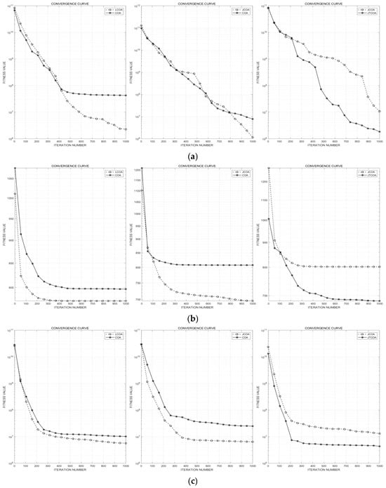
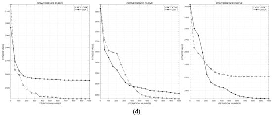
Figure 4. Comparison of convergence curves. (a) Convergence curve for ${\mathrm{F}}_1$; (b) convergence curve for $F_2$; (c) convergence curve for $F_8$; (d) convergence curve for $F_{15}$.

3.3.2. Comparison of DSYCOA with Other Algorithms

This subsection compares the DSYCOA with common algorithms such as the Harris Hawks Optimization (HHO), Beluga Whale Optimization (BWO), Sine-Cosine Algorithm (SCA), Butterfly Optimization Algorithm (BOA), and the pre-improvement Chicken Swarm Optimization Algorithm (COA) to validate its effectiveness. The test results are detailed in Table 3. According to the results, when solving unimodal benchmark test functions, the variance and mean of the results obtained from 30 independent runs of DSYCOA exceed the performance of the other five algorithms, indicating high algorithm stability. Additionally, as shown in Figure 5a, DSYCOA exhibits very fast convergence speed, high convergence accuracy, and good exploitation performance.

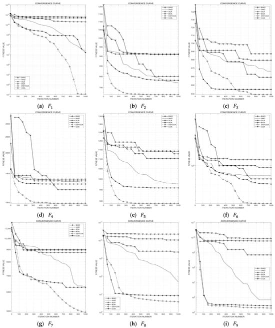
Figure 5. Convergence curves of 21 test functions.

When solving simple multimodal benchmark test functions, DSYCOA achieves optimal mean and variance values compared to the other five algorithms across five test functions ($F_2, F_3, F_4, F_5 \mathrm{a}\mathrm{n}\mathrm{d}{ F}_7$) based on 30 independent runs. For function $F_6$, although DSYCOA’s variance does not reach the best among the six algorithms, the difference is small, and its mean value is optimal. Furthermore, as illustrated in Figure 5b–g, DSYCOA demonstrates the fastest convergence speed and highest convergence accuracy on test functions $F_2$, $F_{4 }\mathrm{a}\mathrm{n}\mathrm{d}{ F}_5$. On test functions $F_3$ and $F_5$, even though DSYCOA’s convergence speed is not the fastest, it has a strong capability to escape local optima and achieves high convergence accuracy.

When solving composite and mixed functions, DSYCOA performs exceptionally well, with the mean and variance of the results from 30 independent runs being optimal among the six algorithms. Moreover, as seen in Figure 5h–u, DSYCOA exhibits superior global search capability, while the other five algorithms are prone to falling into local optima. Especially for test functions $F_{10}, F_{12}, F_{15}, F_{17}, F_{18},$ and $F_{20}$, DSYCOA achieves not only the highest convergence accuracy but also the fastest convergence speed.

4. Simulation Experiments

To confirm the efficacy of the proposed algorithm DSYCOA in optimizing the parameters of the ELM prediction model, this paper tests the upgraded ELM model by means of DSYCOA (DSYCOA-ELM), the refined ELM model via the Harris Hawks Optimization algorithm (HHO [30]-ELM), the modified ELM model using the Black widow optimization algorithm (BWO [31]-ELM), the advanced ELM model by the Butterfly Optimization Algorithm (BOA [32]-ELM), and the boosted ELM model utilizing the Sine Cosine Algorithm (SCA [33]-ELM) using actual power load data from a regional grid. The parameter settings for the ELM are as follows: The network structure adopts a single hidden layer with 30 neurons, the activation function is Sigmoid. The number of input layer nodes is automatically determined by the data (606 nodes), and the output layer has 96 nodes corresponding to the 96 load points of a day. During data preprocessing, the input data is constructed using a sliding window with 6 consecutive days of historical data to predict the next day’s load, and the training set contains 60 days of samples. Input data is normalized to [0, 1], and output data is normalized to [−1, 1]. The parameters for the optimization algorithms follow the original literature recommendations: population size is 30, and maximum iterations are 1000.

Four evaluation metrics, namely MAE, RMSE, MAPE, and the coefficient of determination (R²), are employed to assess the forecasting results of the models. Among the metrics, lower MAE and MAPE values signify a reduced mean variation between the forecasts and actual values, which is indicative of the model’s higher predictive precision. An RMSE value that is smaller suggests a decreased mean deviation between the predicted and actual figures. In comparison with MAE, RMSE places a more significant emphasis on larger errors, thereby demanding greater accuracy from the model. A higher R² value, closer to 1, means that the model explains more of the variability in the dependent variable, which is a sign of a better fit. The formulas for calculating these four evaluation metrics are presented in Equations (30)–(33). Moreover, to maintain fairness in the experiments, the initial parameters of the ELM are set to be uniform, and parameters such as the initial population and the maximum number of iterations for different algorithms are also standardized.

$$MAE={\displaystyle \frac{1}{m}}{\sum }_{i=1}^m\left(\right|y_i-s_i\left|\right)$$

(30)

$$RMSE=\sqrt{{\displaystyle \frac{1}{m}}{\sum }_{i=1}^m{{(y}_i-s_i)}^2}$$

(31)

$$MAPE={\displaystyle \frac{1}{n}}{\sum }_{i=1}^m\left|{\displaystyle \frac{s_i-y_i}{\overline{y_i}}}\right|\times 100\%$$

(32)

$$R^2=1-{\displaystyle \frac{\sum _{i=1}^m{{(y}_i-s_i)}^2}{\sum _{i=1}^m{{(y}_i-\overline{y})}^2}}$$

(33)

In the equations, $y_i$ denotes the predicted value of the model for the ith data point in the dataset, $s_i$ denotes the actual value of the ith data point in the dataset, m represents the total number of test samples, and $\overline{y}$ denotes the mean of the actual values for all samples in the dataset.

The prediction simulation experiment results are presented in Table 4 and Figure 6, Figure 7, Figure 8, Figure 9, Figure 10 and Figure 11. According to Table 4, it can be observed that the five algorithms, namely DSYCOA, BWO, HHO, BOA, and SCA, all exhibit certain improvement effects on the ELM model. Among them, the DSYCOA_ELM model performs the best, followed by the BOA_ELM model. The remaining three models, in order of effectiveness, are: SCA_ELM model, BWO_ELM model, and HHO_ELM model.

Table 4. Evaluation metrics.

Model	MAPE	MAE	RMSE	${\mathbf{R}}^2$	Rank
ELM	5.88%	365.5229	370.554	0.99805	6
DSYCOA-ELM	0.18163%	11.5356	16.4488	0.99986	1
BWO-ELM	1.2912%	81.3237	93.4432	0.99825	4
HHO-ELM	2.2043%	129.9936	150.1341	0.99703	5
BOA-ELM	0.41188%	27.7587	38.7065	0.99925	2
SCA-ELM	0.56884%	37.3977	49.5867	0.99919	3

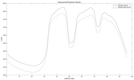
Figure 6. ELM Fitting Plot.

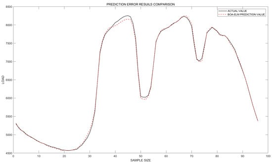
Figure 7. BOA-ELM fitting plot.

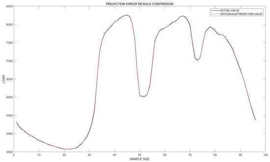
Figure 8. DSYCOA-ELM fitting plot.

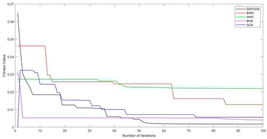
Figure 9. Convergence curve.

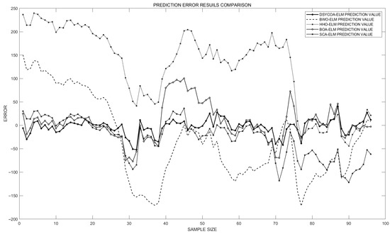
Figure 10. Point-wise prediction discrepancies across models.

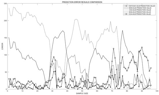
Figure 11. Absolute point-wise prediction errors by model.

In terms of the MAPE evaluation metric, the DSYCOA_ELM model reduces the error by approximately 96.9% and 55.9% compared to the ELM and BOA_ELM models, respectively. For the MAE evaluation metric, the DSYCOA_ELM model decreases the error by about 96.8% and 58.4% compared to the ELM and BOA_ELM models, respectively. In terms of the RMSE evaluation metric, the DSYCOA_ELM model lowers the error by approximately 95.6% and 57.5% compared to the ELM and BOA_ELM models, respectively. Regarding the coefficient of determination (R²), the DSYCOA_ELM model, ELM model, and BOA_ELM model all demonstrate good fitting effects, with the DSYCOA-ELM model exhibiting the highest degree of fitting.

Furthermore, as seen in Figure 9, when optimizing the parameters of the ELM model, SCA demonstrates the fastest convergence speed. Although DSYCOA’s speed is not as fast as SCA’s, it rapidly decreases and stabilizes within 10 iterations. In comparison, BWO, HHO, and BOA converge more slowly relative to SCA and DSYCOA. In terms of solution quality, DSYCOA finds the highest-quality solution, followed by BOA, SCA, BWO, and HHO in descending order. From the perspective of algorithm stability, the curves of DSYCOA and SCA are relatively smooth, indicating good stability during the iteration process. Conversely, the curves of BWO and HHO exhibit larger fluctuations, indicating greater instability in the search for the optimal solution.

As seen in Figure 10 and Figure 11, the prediction error of the DSYCOA_ELM algorithm remains relatively low across the entire range of sample sizes. The prediction errors of the BWO-ELM, HHO-ELM, and SCA_ELM algorithms are higher when the sample size is small. As the sample size increases, these errors decrease, but they still remain higher than those of DSYCOA-ELM, and overall exhibit larger fluctuations. The prediction error of the BOA_ELM algorithm fluctuates significantly across the entire range of sample sizes, particularly when the sample size is between approximately 30 and 70. Considering the findings, it follows that the DSYCOA_ELM model exhibits high stability, strong adaptability to data, effective capture of patterns and trends in data, and good generalization ability. The BWO-ELM, HHO-ELM, and SCA-ELM models tend to overfit when processing short-term power grid load datasets and have a strong dependence on sample size. In contrast, the BOA_ELM algorithm is overly sensitive to certain specific features of the data, resulting in poor stability.

In summary, the DSYCOA_ELM model not only performs outstandingly in the context of predictive accuracy and convergence speed but also demonstrates robustness against outliers and noisy data. It can provide stable and reliable prediction results under the fluctuating and uncertain conditions commonly found in power grid load data, exhibiting significant feasibility and superiority in addressing short-term power load forecasting problems.

5. Conclusions

To achieve precise prediction of immediate power demand in the power grid, thereby ensuring the stable, economic, and efficient operation of the power system, a prediction model based on an improved crayfish algorithm optimized ELM was established. Addressing the shortcomings of the crayfish algorithm, such as low convergence accuracy and susceptibility to local optima, a local adaptive parameter tuning algorithm was proposed and compared with five other algorithms, including the crayfish algorithm, on test functions. Furthermore, simulation experiments were conducted on the power data prediction set for both the proposed model and the ELM models improved by the other algorithms used in the comparison tests. The experimental results demonstrate that the Logistic chaotic mapping strategy can enhance the diversity of the algorithm’s population. The strategies of local precise search and dynamic parameter adjustment can effectively help the algorithm escape from local optima, improving its global search capability. Compared to several other models, the prediction model based on the improved crayfish algorithm optimized ELM not only excels in prediction accuracy and convergence speed but also exhibits strong robustness against outliers and noisy data.

References

- Lin, L.; Liu, J.; Huang, N.; Li, S.; Zhang, Y. Multiscale spatio-temporal feature fusion based non-intrusive appliance load monitoring for multiple industrial industries. Appl. Soft Comput. 2024, 167, 112445. [Google Scholar] [CrossRef]
- Jin, M.; Zhou, X.; Zhang, Z.M.; Tentzeris, M.M. Short-term power load forecasting using grey correlation contest modeling. Expert Syst. Appl. 2012, 39, 773–779. [Google Scholar] [CrossRef]
- Contreras, J.; Espinola, R.; Nogales, F.J.; Conejo, A. ARIMA models to predict next-day electricity prices. IEEE Trans. Power Syst. 2003, 18, 1014–1020. [Google Scholar] [CrossRef]
- Box, G.E.P.; Jenkins, G.M.; Reinsel, G.C.; Ljung, G.M. Time Series Analysis: Forecasting and Control; John Wiley & Sons: Hoboken, NJ, USA, 2015. [Google Scholar]
- Wu, F.; Cattani, C.; Song, W.; Zio, E. Fractional ARIMA with an improved cuckoo search optimization for the efficient Short-term power load forecasting. Alex. Eng. J. 2020, 59, 3111–3118. [Google Scholar] [CrossRef]
- Yuhong, W.; Jie, L. Improvement and application of GM (1, 1) model based on multivariable dynamic optimization. J. Syst. Eng. Electron. 2020, 31, 593–601. [Google Scholar] [CrossRef]
- Barman, M.; Choudhury, N.B.D. A similarity based hybrid GWO-SVM method of power system load forecasting for regional special event days in anomalous load situations in Assam, India. Sustain. Cities Soc. 2020, 61, 102311. [Google Scholar] [CrossRef]
- Dai, Y.; Zhao, P. A hybrid load forecasting model based on support vector machine with intelligent methods for feature selection and parameter optimization. Appl. Energy 2020, 279, 115332. [Google Scholar] [CrossRef]
- Luo, J.; Hong, T.; Gao, Z.; Fang, S.-C. A robust support vector regression model for electric load forecasting. Int. J. Forecast. 2023, 39, 1005–1020. [Google Scholar] [CrossRef]
- Khwaja, A.S.; Anpalagan, A.; Naeem, M.; Venkatesh, B. Joint bagged-boosted artificial neural networks: Using ensemble machine learning to improve short-term electricity load forecasting. Electr. Power Syst. Res. 2020, 179, 106080. [Google Scholar] [CrossRef]
- El Ouadi, J.; Malhene, N.; Benhadou, S.; Medromi, H. Towards a machine-learning based approach for splitting cities in freight logistics context: Benchmarks of clustering and prediction models. Comput. Ind. Eng. 2022, 166, 107975. [Google Scholar] [CrossRef]
- Fan, G.-F.; Zhang, L.-Z.; Yu, M.; Hong, W.-C.; Dong, S.-Q. Applications of random forest in multivariable response surface for short-term load forecasting. Int. J. Electr. Power Energy Syst. 2022, 139, 108073. [Google Scholar] [CrossRef]
- Yazici, I.; Beyca, O.F.; Delen, D. Deep-learning-based short-term electricity load forecasting: A real case application. Eng. Appl. Artif. Intell. 2022, 109, 104645. [Google Scholar] [CrossRef]
- Li, K.; Huang, W.; Hu, G.; Li, J. Ultra-short term power load forecasting based on CEEMDAN-SE and LSTM neural network. Energy Build. 2023, 279, 112666. [Google Scholar] [CrossRef]
- Mounir, N.; Ouadi, H.; Jrhilifa, I. Short-term electric load forecasting using an EMD-BI-LSTM approach for smart grid energy management system. Energy Build. 2023, 288, 113022. [Google Scholar] [CrossRef]
- Lin, J.; Ma, J.; Zhu, J.; Cui, Y. Short-term load forecasting based on LSTM networks considering attention mechanism. Int. J. Electr. Power Energy Syst. 2022, 137, 107818. [Google Scholar] [CrossRef]
- Singh, S.N.; Mohapatra, A. Data driven day-ahead electrical load forecasting through repeated wavelet transform assisted SVM model. Appl. Soft Comput. 2021, 111, 107730. [Google Scholar] [CrossRef]
- Yuqi, J.; An, A.; Lu, Z.; Ping, H.; Xiaomei, L. Short-term load forecasting based on temporal importance analysis and feature extraction. Electr. Power Syst. Res. 2025, 244, 111551. [Google Scholar] [CrossRef]
- Nie, Y.; Jiang, P.; Zhang, H. A novel hybrid model based on combined preprocessing method and advanced optimization algorithm for power load forecasting. Appl. Soft Comput. 2020, 97, 106809. [Google Scholar] [CrossRef]
- Zou, H.; Yang, Q.; Chen, J.; Chai, Y. Short-term power load forecasting based on phase space reconstruction and EMD-ELM. J. Electr. Eng. Technol. 2023, 18, 3349–3359. [Google Scholar] [CrossRef]
- Wang, J.; Niu, X.; Zhang, L.; Liu, Z.; Huang, X. A wind speed forecasting system for the construction of a smart grid with two-stage data processing based on improved ELM and deep learning strategies. Expert Syst. Appl. 2024, 241, 122487. [Google Scholar] [CrossRef]
- Loizidis, S.; Kyprianou, A.; Georghiou, G.E. Electricity market price forecasting using ELM and Bootstrap analysis: A case study of the German and Finnish Day-Ahead markets. Appl. Energy 2024, 363, 123058. [Google Scholar] [CrossRef]
- Wu, C.; Li, J.; Liu, W.; He, Y.; Nourmohammadi, S. Short-term electricity demand forecasting using a hybrid ANFIS–ELM network optimised by an improved parasitism–predation algorithm. Appl. Energy 2023, 345, 121316. [Google Scholar] [CrossRef]
- Rayi, V.K.; Mishra, S.P.; Naik, J.; Dash, P. Adaptive VMD based optimized deep learning mixed kernel ELM autoencoder for single and multistep wind power forecasting. Energy 2022, 244, 122585. [Google Scholar] [CrossRef]
- Li, C.; Zhou, J.; Tao, M.; Du, K.; Wang, S.; Armaghani, D.J.; Mohamad, E.T. Developing hybrid ELM-ALO, ELM-LSO and ELM-SOA models for predicting advance rate of TBM. Transp. Geotech. 2022, 36, 100819. [Google Scholar] [CrossRef]
- Ma, R.; Karimzadeh, M.; Ghabussi, A.; Zandi, Y.; Baharom, S.; Selmi, A.; Maureira-Carsalade, N. Assessment of composite beam performance using GWO–ELM metaheuristic algorithm. Eng. Comput. 2021, 38, 2083–2099. [Google Scholar] [CrossRef]
- Wang, J.; Zhang, Y.; Zhang, F.; Li, W.; Lv, S.; Jiang, M.; Jia, L. Accuracy-improved bearing fault diagnosis method based on AVMD theory and AWPSO-ELM model. Measurement 2021, 181, 109666. [Google Scholar] [CrossRef]
- Shariati, M.; Mafipour, M.S.; Ghahremani, B.; Azarhomayun, F.; Ahmadi, M.; Trung, N.T.; Shariati, A. A novel hybrid extreme learning machine–grey wolf optimizer (ELM-GWO) model to predict compressive strength of concrete with partial replacements for cement. Eng. Comput. 2022, 38, 757–779. [Google Scholar] [CrossRef]
- Ikram, R.M.A.; Dai, H.-L.; Chargari, M.M.; Al-Bahrani, M.; Mamlooki, M. Prediction of the FRP reinforced concrete beam shear capacity by using ELM-CRFOA. Measurement 2022, 205, 112230. [Google Scholar] [CrossRef]
- Heidari, A.A.; Mirjalili, S.; Faris, H.; Aljarah, I.; Mafarja, M.; Chen, H. Harris hawks optimization: Algorithm and applications. Future Gener. Comput. Syst. 2019, 97, 849–872. [Google Scholar] [CrossRef]
- Hayyolalam, V.; Kazem, A.A.P. Black widow optimization algorithm: A novel meta-heuristic approach for solving engineering optimization problems. Eng. Appl. Artif. Intell. 2020, 87, 103249. [Google Scholar] [CrossRef]
- Arora, S.; Singh, S. Butterfly optimization algorithm: A novel approach for global optimization. Soft Comput. 2019, 23, 715–734. [Google Scholar] [CrossRef]
- Mirjalili, S. SCA: A sine cosine algorithm for solving optimization problems. Knowl.-Based Syst. 2016, 96, 120–133. [Google Scholar] [CrossRef]
Disclaimer/Publisher’s Note: The statements, opinions and data contained in all publications are solely those of the individual author(s) and contributor(s) and not of MDPI and/or the editor(s). MDPI and/or the editor(s) disclaim responsibility for any injury to people or property resulting from any ideas, methods, instructions or products referred to in the content. |
© 2025 by the authors. Licensee MDPI, Basel, Switzerland. This article is an open access article distributed under the terms and conditions of the Creative Commons Attribution (CC BY) license (https://creativecommons.org/licenses/by/4.0/).