
3D UAV Route Optimization in Complex Environments Using an Enhanced Artificial Lemming Algorithm


Abstract
1. Introduction
- (1)
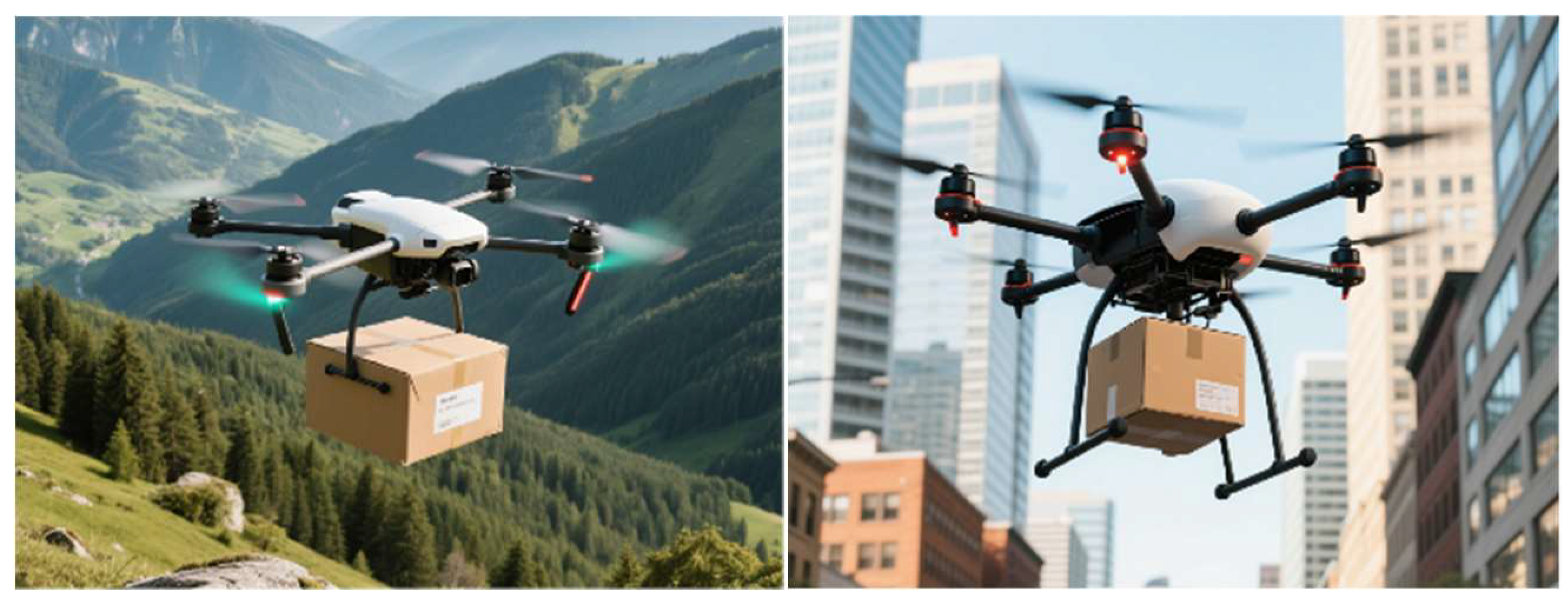
- A multi-environment UAV logistics delivery route planning model was constructed. This model is capable of simulating the logistics delivery environments in mountainous and urban areas.
- (2)
- In an urban environment, the environment is only rasterized in a two-dimensional space and the restriction that candidate points can only be at the grid centers is removed, allowing the UAV to select route points more freely and, thus, conforming it to the actual delivery environments.
- (3)
- Aiming at the problem that the artificial lemming algorithm (ALA) is prone to falling into local optimal solutions, three improvement strategies were applied to the original ALA algorithm, thus forming a new multi-strategy improved artificial lemming algorithm (MsIALA).
- (4)
- The improved algorithm was perfectly integrated with the proposed model, demonstrating the effectiveness and high efficiency of the algorithm and providing a certain reference for the 3D route planning of UAV logistics delivery.
2. Multi-Environment Logistics Delivery Route Planning Model Based on UAV
2.1. Environmental Model
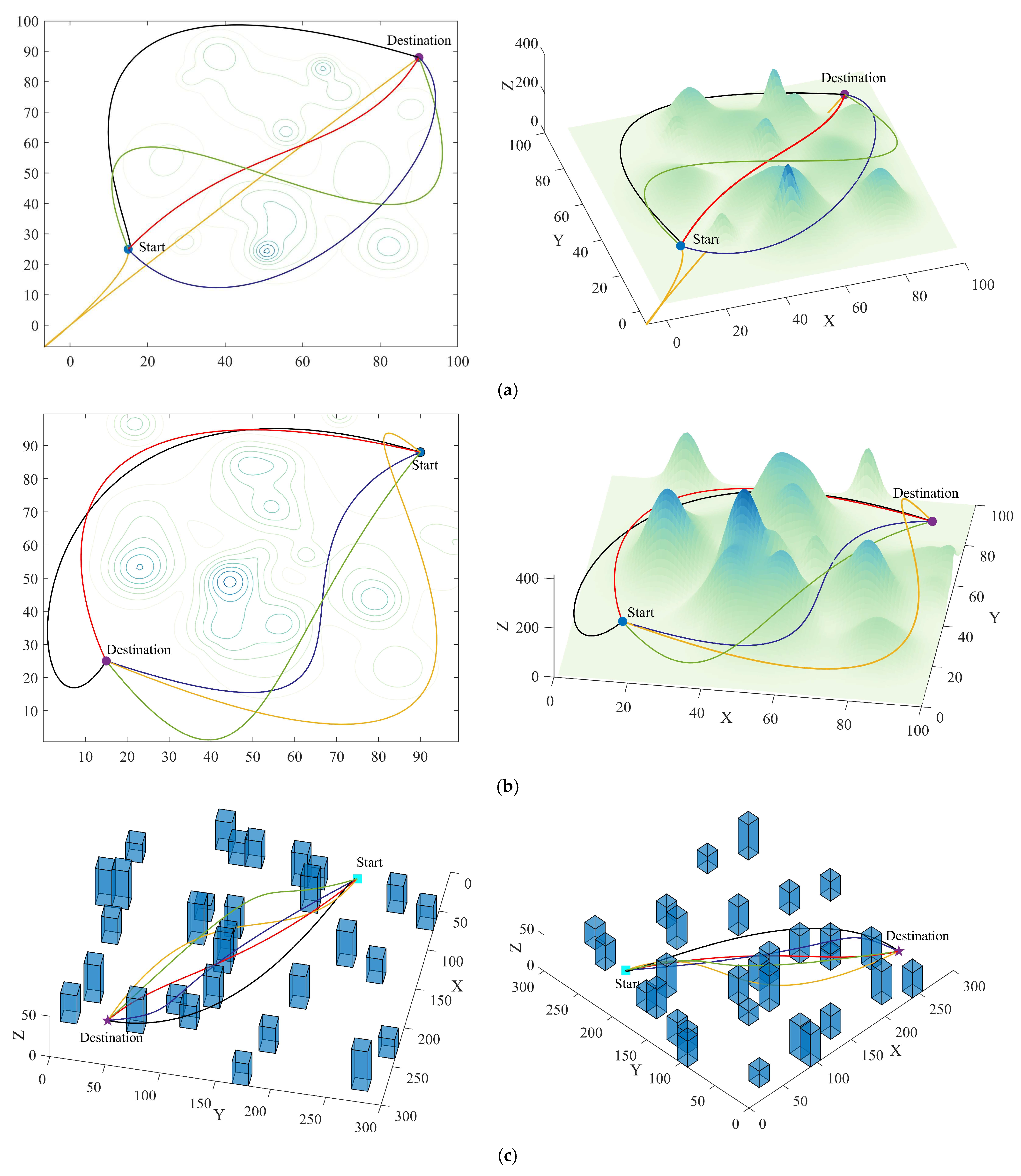
- (a)
- Mountainous environments
- (b)
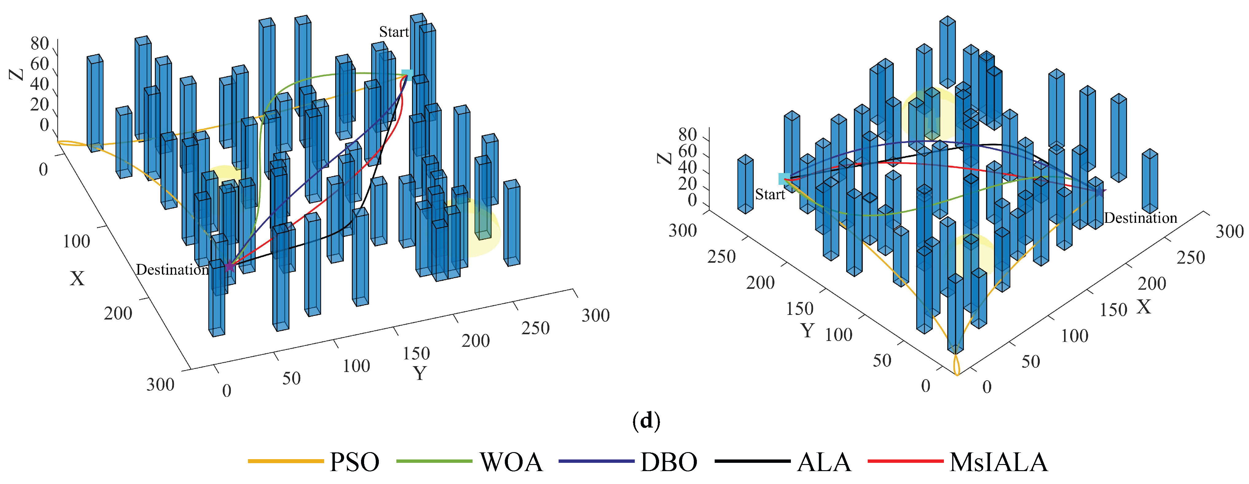
- Urban environments
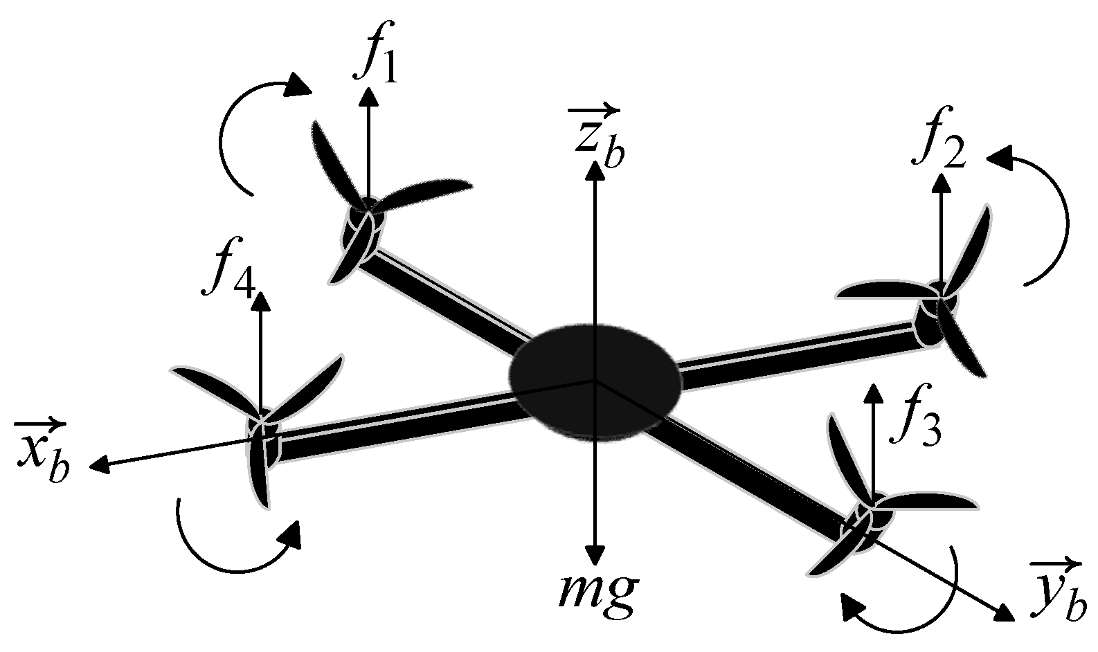
2.2. UAV Dynamics Model
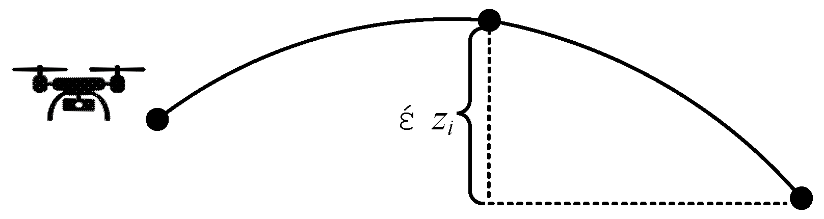
2.3. Route Generation and Smoothing
2.3.1. Encoding and Decoding
- (a)
- The x-coordinates of all points are sequentially placed in the first positions.
- (b)
- The y-coordinates are placed in the middle positions.
- (c)
- The z-coordinates occupy the last positions.
2.3.2. Cubic Spline Interpolation
- (a)
- ;
- (b)
- (c)
- On each sub-interval , is a cubic polynomial.
2.4. UAV Logistics Delivery 3D Route Planning Model
2.4.1. Cost Function Design
- (a)
- Route length
- (b)
- Flight fluctuation
2.4.2. Constraints
- (a)
- Flight length
- (b)
- Goods weight
- (c)
- Yaw angle constraint
- (d)
- Pitch angle constraint
- (e)
- Obstacle constraint
3. Multi-Strategy Improved Artificial Lemming Algorithm
3.1. Principle of Artificial Lemming Algorithm
- (a)
- Long-distance migration
- (b)
- Digging holes
- (c)
- Foraging
- (d)
- Evading predators
3.2. Improvement Strategies
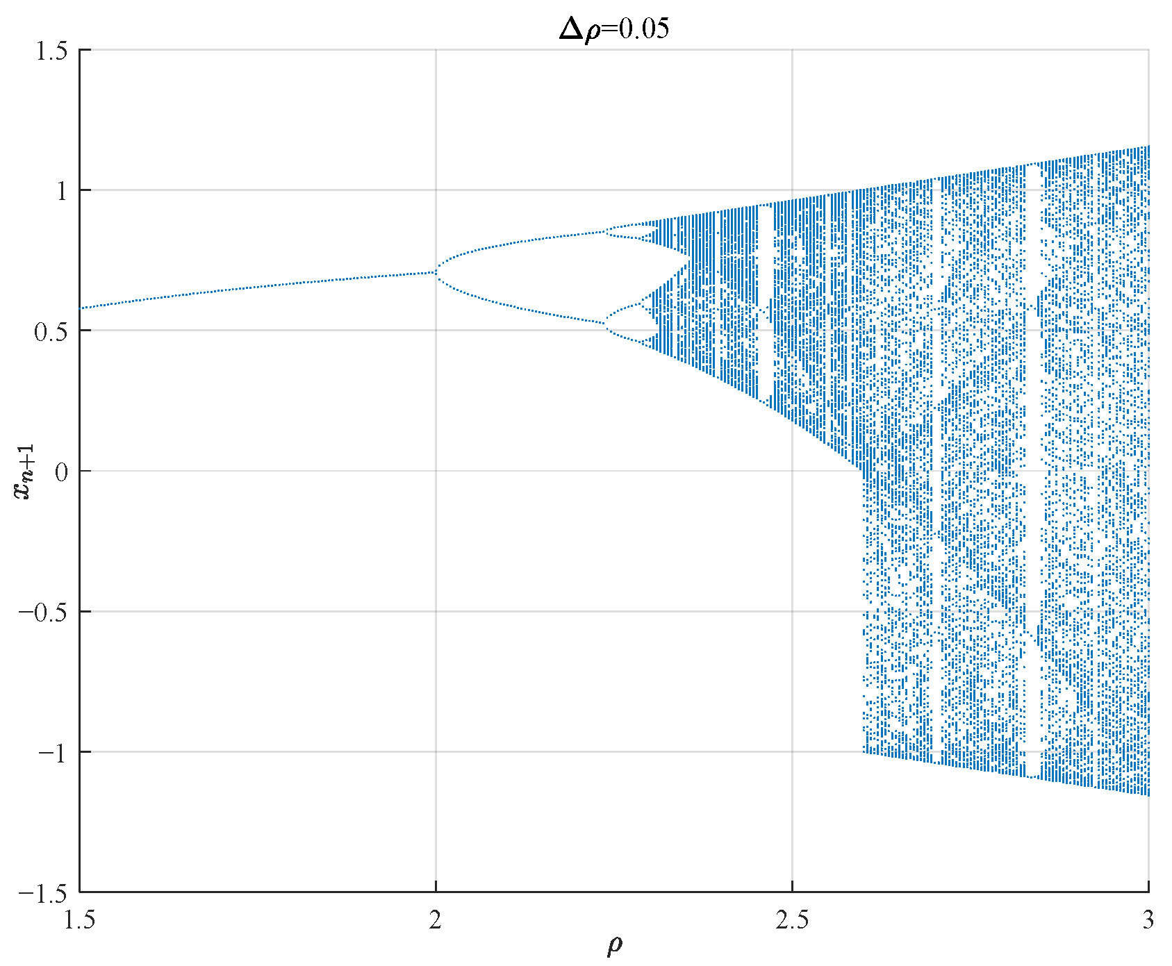
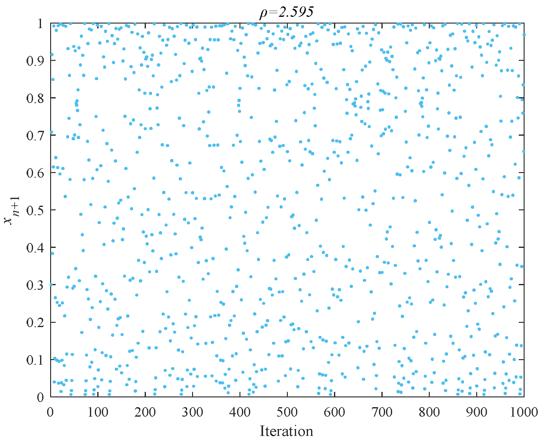
3.2.1. Cubic Chaotic Map Initialization
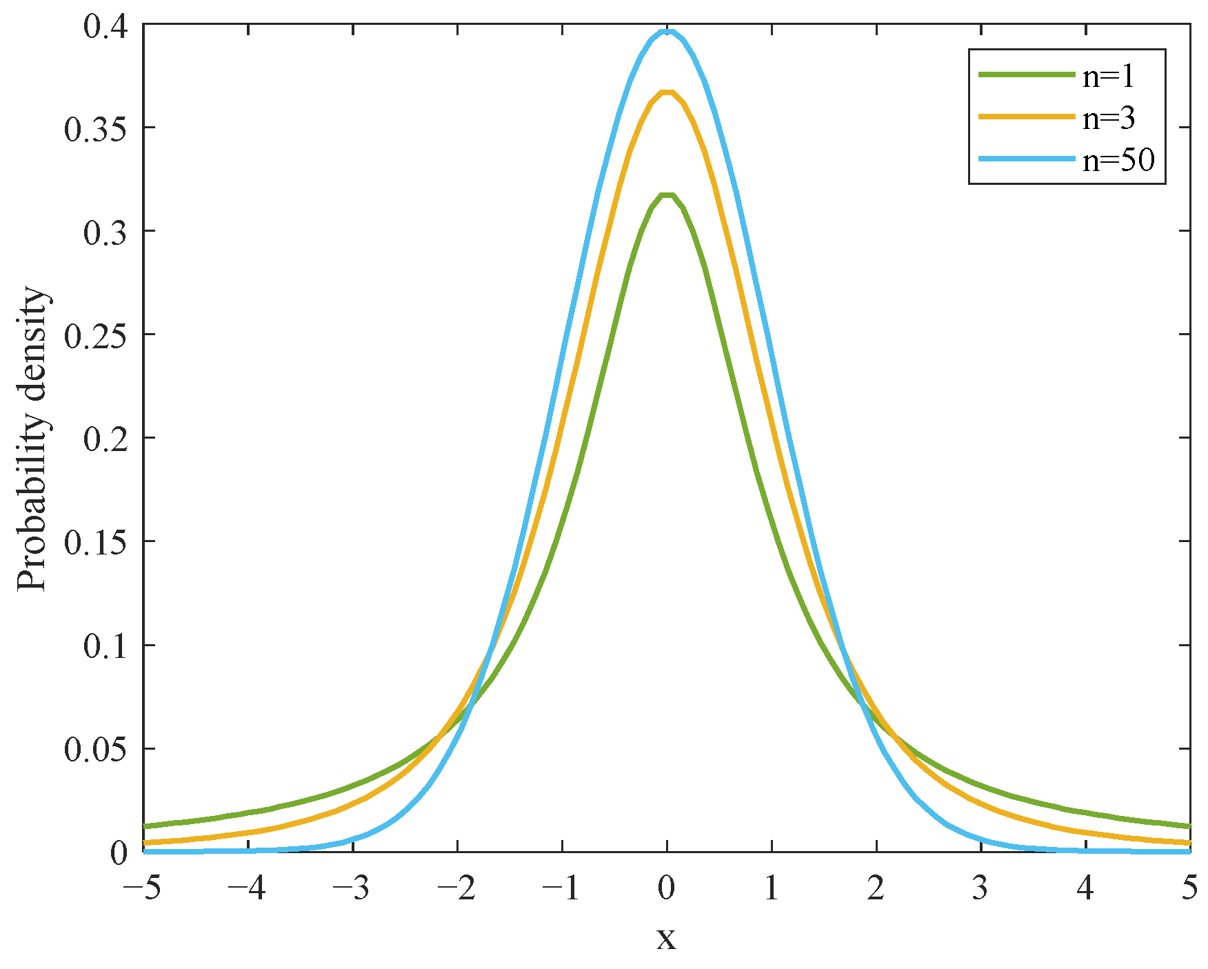
3.2.2. Double Adaptive T-Distribution Perturbation
3.2.3. Population Dynamic Optimization
3.3. Algorithm Flow and Computational Complexity
| Algorithm 1. Multi-strategy improved artificial lemming algorithm. |
| Input: The maximum iterations ; the size of the population ; the dimension size . |
Output: The optimal position ; the optimal fitness value .
|
|
3.4. Data Experiment
4. Simulation Experiment and Result Analysis
4.1. Experimental Environment and Parameter Settings
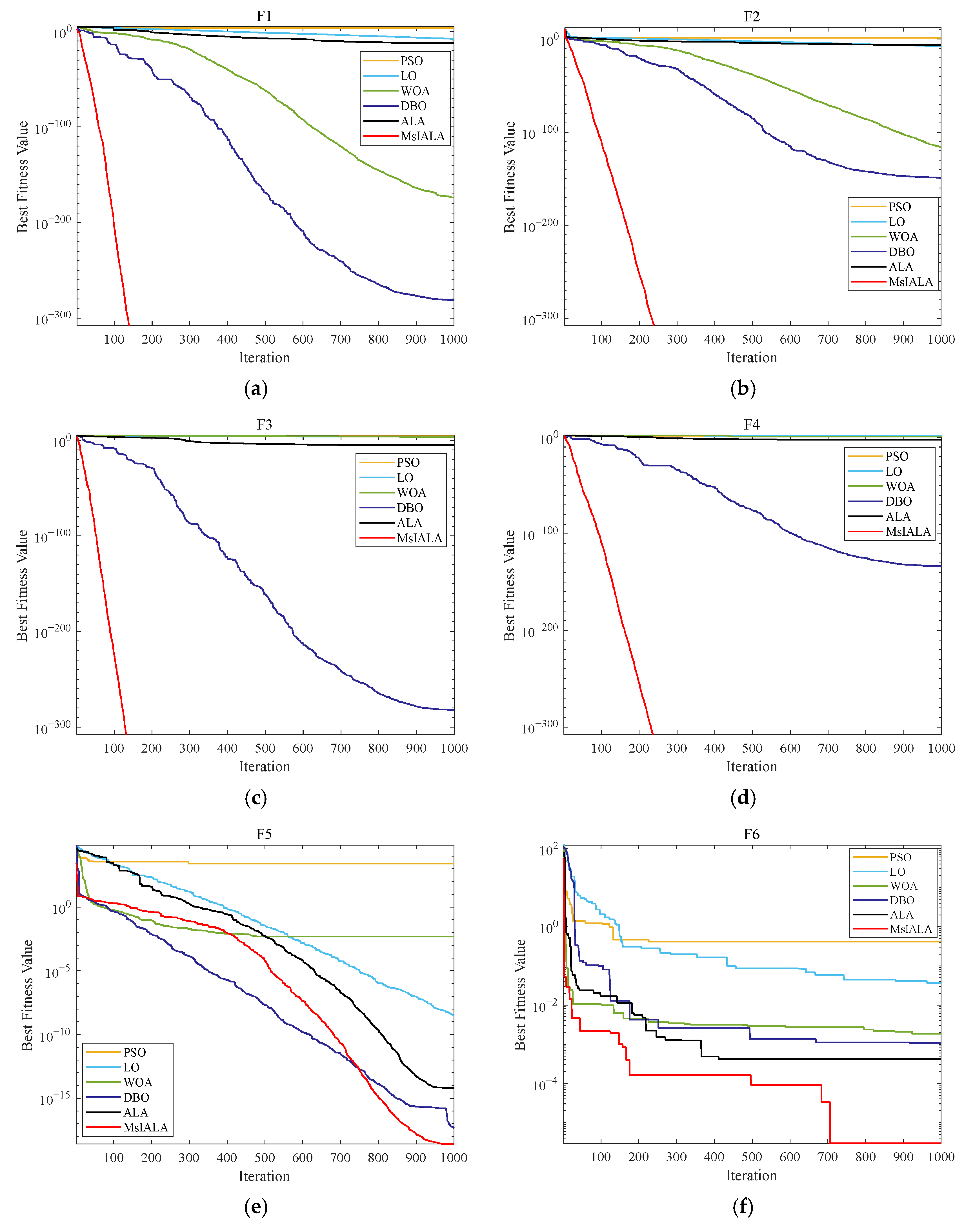
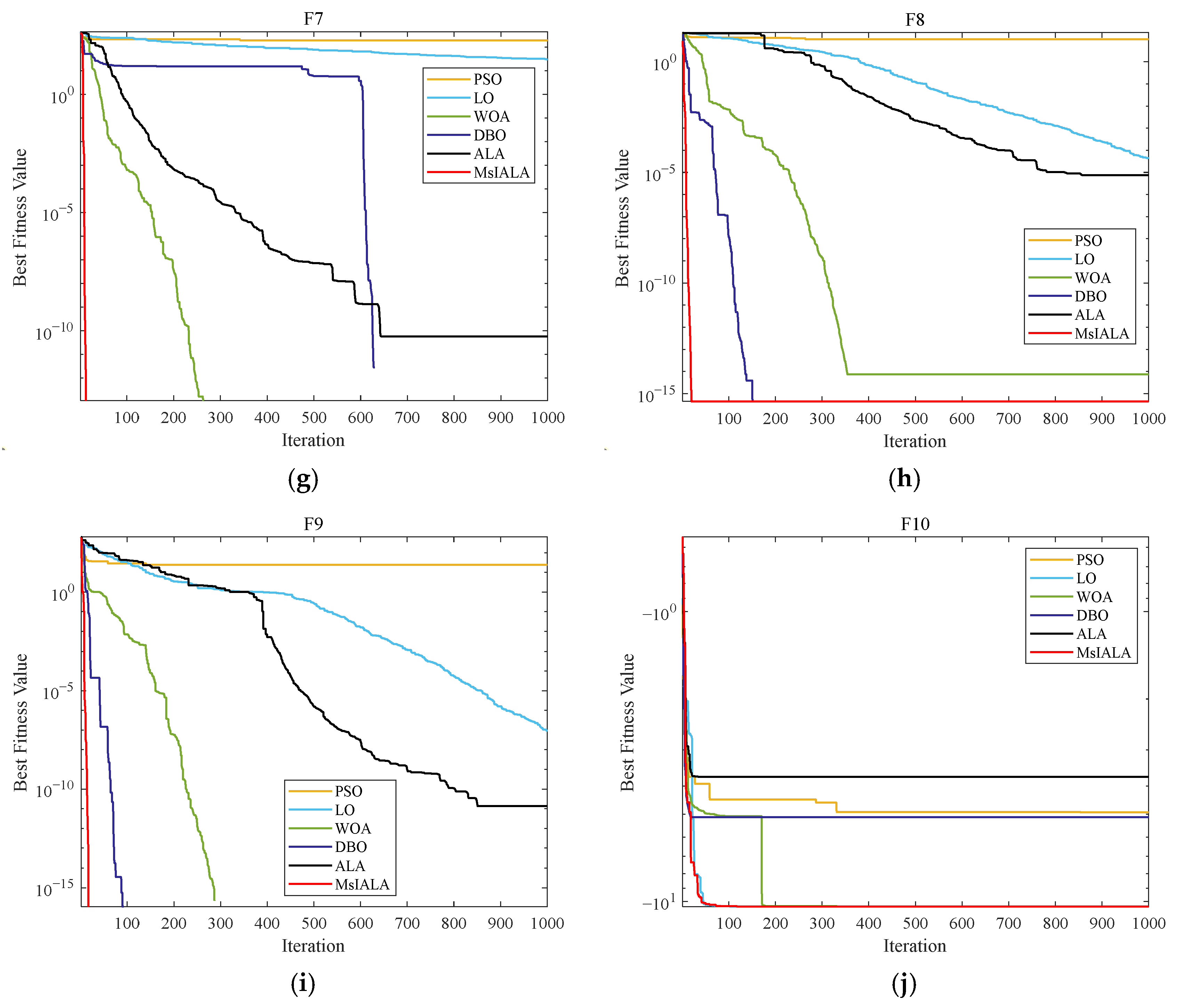
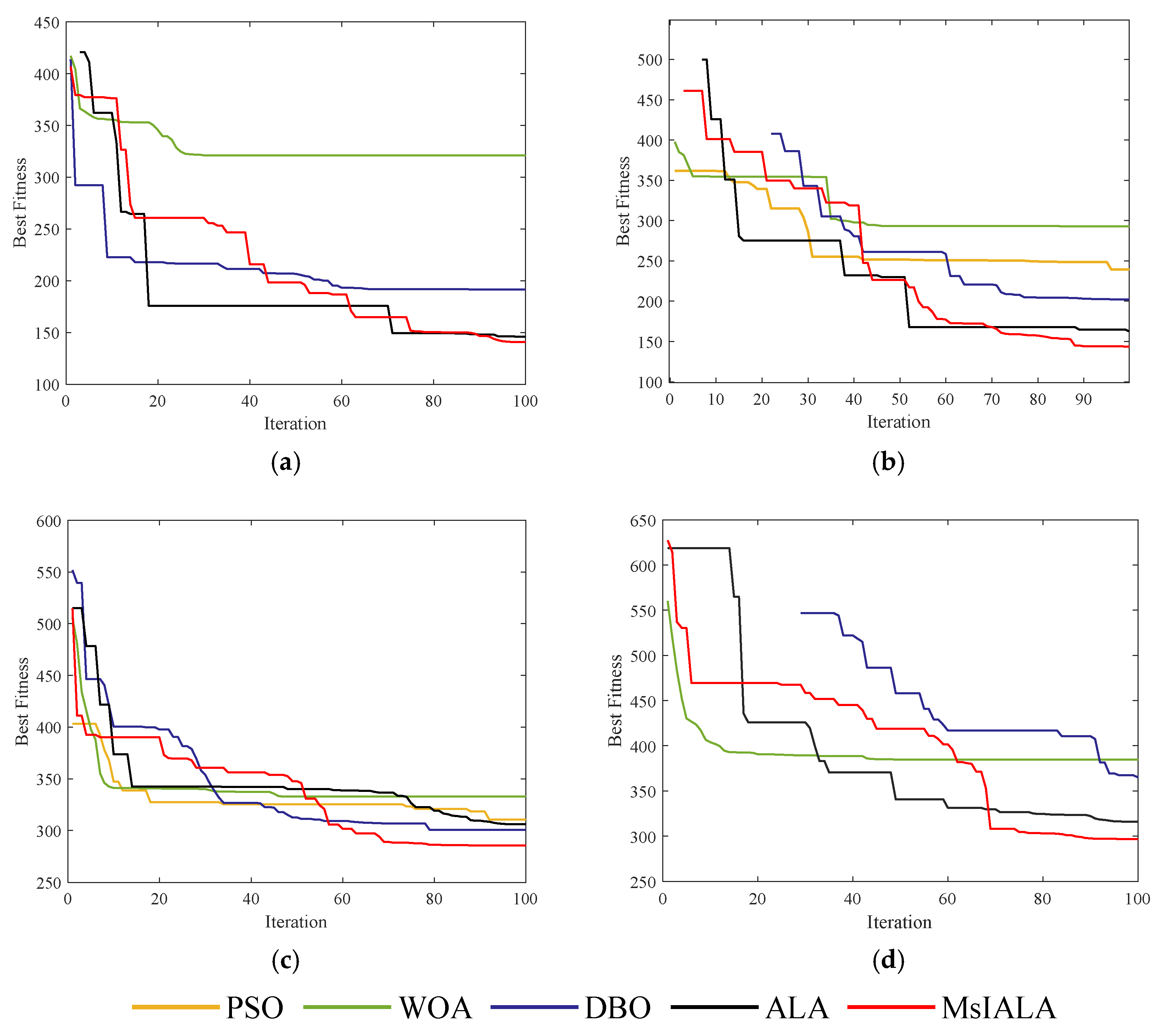
4.2. Experimental Results
4.3. Stability Analysis
5. Summary and Outlook
Author Contributions
Funding
Data Availability Statement
Conflicts of Interest
References
- Fried, T.; Goodchild, A. E-commerce and logistics sprawl: A spatial exploration of last-mile logistics platforms. J. Transp. Geogr. 2023, 112, 103692. [Google Scholar] [CrossRef]
- Lee, H.-W. Research on multi-functional logistics intelligent Unmanned Aerial Vehicle. Eng. Appl. Artif. Intell. 2022, 116, 105341. [Google Scholar] [CrossRef]
- Mohamed, N.; Al-Jaroodi, J.; Jawhar, I.; Idries, A.; Mohammed, F. Unmanned aerial vehicles applications in future smart cities. Technol. Forecast. Soc. Change 2020, 153, 119293. [Google Scholar] [CrossRef]
- Mandloi, D.; Arya, R.; Verma, A.K. Unmanned aerial vehicle path planning based on A* algorithm and its variants in 3d environment. Int. J. Syst. Assur. Eng. Manag. 2021, 12, 990–1000. [Google Scholar] [CrossRef]
- Li, Z.; Zhang, S. Research on 3D path planning algorithm based on fast RRT algorithm. J. Syst. Simul. 2022, 34, 503–511. [Google Scholar]
- Li, X.; Yu, S. Obstacle avoidance path planning for AUVs in a three-dimensional unknown environment based on the C-APF-TD3 algorithm. Ocean Eng. 2025, 315, 119886. [Google Scholar] [CrossRef]
- Saeed, R.A.; Omri, M.; Abdel-Khalek, S.; Ali, E.S.; Alotaibi, M.F. Optimal path planning for drones based on swarm intelligence algorithm. Neural Comput. Appl. 2022, 34, 10133–10155. [Google Scholar] [CrossRef]
- Phung, M.D.; Ha, Q.P. Safety-enhanced UAV path planning with spherical vector-based particle swarm optimization. Appl. Soft Comput. 2021, 107, 107376. [Google Scholar] [CrossRef]
- Jiang, W.; Lyu, Y.; Li, Y.; Guo, Y.; Zhang, W. UAV path planning and collision avoidance in 3D environments based on POMPD and improved grey wolf optimizer. Aerosp. Sci. Technol. 2022, 121, 107314. [Google Scholar] [CrossRef]
- Yan, Z.; Zhang, J.; Zeng, J.; Tang, J. Three-dimensional path planning for autonomous underwater vehicles based on a whale optimization algorithm. Ocean Eng. 2022, 250, 111070. [Google Scholar] [CrossRef]
- Fu, S.; Li, K.; Huang, H.; Ma, C.; Fan, Q.; Zhu, Y. Red-billed blue magpie optimizer: A novel metaheuristic algorithm for 2D/3D UAV path planning and engineering design problems. Artif. Intell. Rev. 2024, 57, 134. [Google Scholar] [CrossRef]
- Yu, Z.; Si, Z.; Li, X.; Wang, D.; Song, H. A novel hybrid particle swarm optimization algorithm for path planning of UAVs. IEEE Internet Things J. 2022, 9, 22547–22558. [Google Scholar] [CrossRef]
- Liu, Y.; Zhu, X.; Zhang, X.-Y.; Xiao, J.; Yu, X. RGG-PSO+: Random geometric graphs based particle swarm optimization method for UAV path planning. Int. J. Comput. Intell. Syst. 2024, 17, 127. [Google Scholar] [CrossRef]
- Liang, H.; Hu, W.; Gong, K.; Dai, J.; Wang, L. Solving UAV 3D Path Planning Based on the Improved Lemur Optimizer Algorithm. Biomimetics 2024, 9, 654. [Google Scholar] [CrossRef]
- Shen, Q.; Zhang, D.; Xie, M.; He, Q. Multi-Strategy enhanced dung beetle optimizer and its application in three-dimensional UAV path planning. Symmetry 2023, 15, 1432. [Google Scholar] [CrossRef]
- Wang, R.-B.; Wang, W.-F.; Geng, F.-D.; Pan, J.-S.; Chu, S.-C.; Xu, L. UAV path planning in mountain areas based on a hybrid parallel compact arithmetic optimization algorithm. Neural Comput. Appl. 2023, 1–16. [Google Scholar] [CrossRef]
- Mahony, R.; Kumar, V.; Corke, P. Multirotor Aerial Vehicles: Modeling, Estimation, and Control of Quadrotor. IEEE Robot. Autom. Mag. 2012, 19, 20–32. [Google Scholar] [CrossRef]
- McKinley, S.; Levine, M. Cubic spline interpolation. Coll. Redw. 1998, 45, 1049–1060. [Google Scholar]
- Xiao, Y.; Cui, H.; Abu Khurma, R.; Castillo, P.A. Artificial lemming algorithm: A novel bionic meta-heuristic technique for solving real-world engineering optimization problems. Artif. Intell. Rev. 2025, 58, 84. [Google Scholar] [CrossRef]
- Yuan, X.; Zhao, J.; Yang, Y.; Wang, Y. Hybrid parallel chaos optimization algorithm with harmony search algorithm. Appl. Soft Comput. 2014, 17, 12–22. [Google Scholar] [CrossRef]
- Kennedy, J.; Eberhart, R. Particle swarm optimization. In Proceedings of the ICNN’95-International Conference on Neural Networks, Perth, WA, Australia, 27 November–1 December 1995; IEEE: Piscataway, NJ, USA, 1995; Volume 4, pp. 1942–1948. [Google Scholar]
- Abasi, A.K.; Makhadmeh, S.N.; Al-Betar, M.A.; Alomari, O.A.; Awadallah, M.A.; Alyasseri, Z.A.A.; Abu Doush, I.; Elnagar, A.; Alkhammash, E.H.; Hadjouni, M. Lemurs optimizer: A new metaheuristic algorithm for global optimization. Appl. Sci. 2022, 12, 10057. [Google Scholar] [CrossRef]
- Mirjalili, S.; Lewis, A. The whale optimization algorithm. Adv. Eng. Softw. 2016, 95, 51–67. [Google Scholar] [CrossRef]
- Xue, J.; Shen, B. Dung beetle optimizer: A new meta-heuristic algorithm for global optimization. J. Supercomput. 2023, 79, 7305–7336. [Google Scholar] [CrossRef]


| Function | Dimension | Variable Interval | Theoretical Best |
|---|---|---|---|
| 30 | [−100, 100] | 0 | |
| 30 | [−10, 10] | 0 | |
| 30 | [−100, 100] | 0 | |
| 30 | [−100, 100] | 0 | |
| 30 | [−100, 100] | 0 | |
| 30 | [−1.28, 1.28] | 0 | |
| 30 | [−5.12, 5.12] | 0 | |
| 30 | [−32, 32] | 0 | |
| 30 | [−600, 600] | 0 | |
| 4 | [0, 10] | −10 |
| Function | Index | PSO [21] | LO [22] | WOA [23] | DBO [24] | ALA [19] | MsIALA |
|---|---|---|---|---|---|---|---|
| F1 | min | 3.3242 × 10⁻⁷ | 2.4920 × 10⁻⁹ | 2.6029 × 10−191 | 0 | 1.0525 × 10⁻¹³ | 0 |
| avg | 6.9896 × 10⁻⁶ | 9.9626 × 10⁻⁹ | 8.7434 × 10−173 | 4.4799 × 10−242 | 4.2962 × 10⁻¹² | 0 | |
| std | 6.0767 × 10⁻⁶ | 6.7974 × 10⁻⁹ | 0 | 0 | 6.4890 × 10⁻¹² | 0 | |
| rank | 6 | 5 | 3 | 2 | 4 | 1 | |
| F2 | min | 1.0305 × 10⁻⁵ | 1.2161 × 10⁻⁸ | 4.7842 × 10−118 | 3.4470 × 10−164 | 4.3032 × 10⁻⁸ | 0 |
| avg | 9.5755 × 10⁻⁵ | 3.6532 × 10⁻⁸ | 3.6048 × 10−108 | 7.7406 × 10−116 | 7.4625 × 10⁻⁷ | 0 | |
| std | 7.7301 × 10⁻⁵ | 2.1566 × 10⁻⁸ | 1.5532 × 10−107 | 4.2394 × 10−115 | 1.0019 × 10⁻⁶ | 0 | |
| rank | 6 | 4 | 3 | 2 | 5 | 1 | |
| F3 | min | 1.0758 × 10² | 3.6240 × 10³ | 9.0110 × 101 | 1.6612 × 10−302 | 5.2294 × 10⁻⁷ | 0 |
| avg | 2.9602 × 10² | 6.8778 × 10³ | 1.1289 × 10⁴ | 1.0380 × 10−81 | 8.5696 × 10⁻⁶ | 0 | |
| std | 1.5206 × 10² | 2.3929 × 10³ | 7.9584 × 10³ | 5.6854 × 10−81 | 5.9557 × 10⁻⁶ | 0 | |
| rank | 4 | 5 | 6 | 2 | 3 | 1 | |
| F4 | min | 1.6186 | 1.3287 × 101 | 3.8734 × 10⁻² | 2.9150 × 10−159 | 1.2411 × 10⁻³ | 0 |
| avg | 3.2801 | 2.5391 × 101 | 2.4754 × 101 | 9.9028 × 10−111 | 2.0928 × 10⁻³ | 0 | |
| std | 9.3955 × 10⁻¹ | 5.9376 | 2.5915 × 101 | 5.4240 × 10−110 | 5.1219 × 10⁻⁴ | 0 | |
| rank | 4 | 6 | 5 | 2 | 3 | 1 | |
| F5 | min | 9.0341 × 10⁻⁸ | 7.9580 × 10⁻¹⁰ | 9.9785 × 10⁻⁴ | 4.3750 × 10⁻²⁰ | 1.8851 × 10⁻¹⁷ | 1.5155 × 10⁻¹⁹ |
| avg | 1.5058 × 10⁻⁵ | 1.5998 × 10⁻⁸ | 1.0662 × 10⁻² | 1.1032 × 10⁻¹⁷ | 6.4047 × 10⁻¹⁵ | 7.8822 × 10⁻¹⁸ | |
| std | 4.8925 × 10⁻⁵ | 1.8316 × 10⁻⁸ | 3.6293 × 10⁻² | 2.0447 × 10⁻¹⁷ | 2.8089 × 10⁻¹⁴ | 1.1270 × 10⁻¹⁷ | |
| rank | 5 | 4 | 6 | 2 | 3 | 1 | |
| F6 | min | 9.0231 × 10⁻³ | 1.3055 × 10⁻² | 1.6601 × 10⁻⁵ | 9.3644 × 10⁻⁵ | 4.1837 × 10⁻⁵ | 6.3925 × 10⁻⁷ |
| avg | 1.9319 × 10⁻² | 3.5652 × 10⁻² | 1.1118 × 10⁻³ | 9.7710 × 10⁻⁴ | 8.4487 × 10⁻⁴ | 3.8916 × 10⁻⁵ | |
| std | 5.6102 × 10⁻³ | 1.2317 × 10⁻² | 1.1345 × 10⁻³ | 8.8982 × 10⁻⁴ | 6.7041 × 10⁻⁴ | 3.4013 × 10⁻⁵ | |
| rank | 5 | 6 | 4 | 3 | 2 | 1 | |
| F7 | min | 2.0036 × 101 | 1.5477 × 101 | 0 | 0 | 2.6205 × 10⁻¹¹ | 0 |
| avg | 3.7507 × 101 | 3.0337 × 101 | 0 | 1.2409 × 101 | 2.3216 × 10⁻¹ | 0 | |
| std | 1.0367 × 101 | 8.3687 | 0 | 3.8427 × 101 | 5.0147 × 10⁻¹ | 0 | |
| rank | 5 | 4 | 1 | 3 | 2 | 1 | |
| F8 | min | 1.3568 × 10⁻⁴ | 8.9129 × 10⁻⁶ | 4.4409 × 10⁻¹⁶ | 4.4409 × 10⁻¹⁶ | 3.6721 × 10⁻⁷ | 4.4409 × 10⁻¹⁶ |
| avg | 8.5912 × 10⁻⁴ | 3.2615 × 10⁻⁵ | 3.0494 × 10⁻¹⁵ | 5.6251 × 10⁻¹⁶ | 6.8409 × 10⁻⁶ | 4.4409 × 10⁻¹⁶ | |
| std | 7.3137 × 10⁻⁴ | 1.3461 × 10⁻⁵ | 2.0723 × 10⁻¹⁵ | 6.4863 × 10⁻¹⁶ | 9.8553 × 10⁻⁶ | 0 | |
| rank | 6 | 5 | 2 | 3 | 4 | 1 | |
| F9 | min | 1.1316 × 10⁻⁶ | 1.2785 × 10⁻⁸ | 0 | 0 | 2.1755 × 10⁻¹² | 0 |
| avg | 1.8485 × 10⁻² | 4.7617 × 10⁻³ | 1.2419 × 10⁻³ | 3.3561 × 10⁻³ | 5.8549 × 10⁻¹¹ | 0 | |
| std | 2.4299 × 10⁻² | 7.6158 × 10⁻³ | 6.8020 × 10⁻³ | 1.2966 × 10⁻² | 8.0085 × 10⁻¹¹ | 0 | |
| rank | 6 | 5 | 3 | 4 | 2 | 1 | |
| F10 | min | −1.0403 × 101 | −1.0403 × 101 | −1.0403 × 101 | −1.0403 × 101 | −1.0403 × 101 | −1.0403 × 101 |
| avg | −7.9169 | −1.0403 × 101 | −9.7937 | −7.6334 | −9.6488 | −1.0403 × 101 | |
| std | 3.4054 | 4.5308 × 10⁻¹² | 1.8909 | 2.8565 | 1.9678 | 9.8958 × 10⁻¹⁶ | |
| rank | 4 | 1 | 2 | 5 | 3 | 1 |
| Parameter | Value | Parameter | Value |
|---|---|---|---|
| /km | 5 | π/2 | |
| /kg | 10 | α1 | 0.6 |
| π/2 | α2 | 0.4 |
| Environment | Algorithm | PSO | WOA | DBO | ALA | MsIALA | |
|---|---|---|---|---|---|---|---|
| Index | |||||||
| Mountainous 1 | min | 156.87 | 231.39 | 141.58 | 143.65 | 143.71 | |
| avg | 199.96 | 294.18 | 193.72 | 168.17 | 160.44 | ||
| std | 46.99 | 60.76 | 36.74 | 22.51 | 11.78 | ||
| failure rate | 26.67% | 36.67% | 0 | 0 | 0 | ||
| Mountainous 2 | min | 155.75 | 150.68 | 140.54 | 141.96 | 140.42 | |
| avg | 247.42 | 261.66 | 203.13 | 195.92 | 167.42 | ||
| std | 64.60 | 71.50 | 50.46 | 37.66 | 17.61 | ||
| failure rate | 56.67% | 53.33% | 6.67% | 10.00% | 0 | ||
| Urban 1 | min | 293.18 | 293.35 | 286.11 | 286.06 | 285.44 | |
| avg | 302.68 | 322.07 | 297.61 | 299.52 | 290.34 | ||
| std | 6.41 | 13.87 | 11.75 | 12.05 | 5.85 | ||
| failure rate | 0 | 0 | 0 | 0 | 0 | ||
| Urban 2 | min | 301.67 | 299.01 | 296.25 | 295.73 | 294.34 | |
| avg | 315.88 | 347.65 | 320.47 | 323.74 | 301.98 | ||
| std | 12.96 | 30.93 | 43.42 | 23.39 | 7.61 | ||
| failure rate | 23.33% | 43.33% | 0 | 3.33% | 0 | ||
Disclaimer/Publisher’s Note: The statements, opinions and data contained in all publications are solely those of the individual author(s) and contributor(s) and not of MDPI and/or the editor(s). MDPI and/or the editor(s) disclaim responsibility for any injury to people or property resulting from any ideas, methods, instructions or products referred to in the content. |
© 2025 by the authors. Licensee MDPI, Basel, Switzerland. This article is an open access article distributed under the terms and conditions of the Creative Commons Attribution (CC BY) license (https://creativecommons.org/licenses/by/4.0/).
Share and Cite
Xie, Y.; Sun, Z.; Yuan, K.; Sun, Z. 3D UAV Route Optimization in Complex Environments Using an Enhanced Artificial Lemming Algorithm. Symmetry 2025, 17, 946. https://doi.org/10.3390/sym17060946
Xie Y, Sun Z, Yuan K, Sun Z. 3D UAV Route Optimization in Complex Environments Using an Enhanced Artificial Lemming Algorithm. Symmetry. 2025; 17(6):946. https://doi.org/10.3390/sym17060946
Chicago/Turabian StyleXie, Yuxuan, Zhe Sun, Kai Yuan, and Zhixin Sun. 2025. "3D UAV Route Optimization in Complex Environments Using an Enhanced Artificial Lemming Algorithm" Symmetry 17, no. 6: 946. https://doi.org/10.3390/sym17060946
APA StyleXie, Y., Sun, Z., Yuan, K., & Sun, Z. (2025). 3D UAV Route Optimization in Complex Environments Using an Enhanced Artificial Lemming Algorithm. Symmetry, 17(6), 946. https://doi.org/10.3390/sym17060946