Article

An Improved NSGA-II for Three-Stage Distributed Heterogeneous Hybrid Flowshop Scheduling with Flexible Assembly and Discrete Transportation

by
Zhiyuan Shi
1,
Haojie Chen
2,*,
Fuqian Yan
1,
Xutao Deng
1,
Haiqiang Hao
3,
Jialei Zhang
1 and
Qingwen Yin
1
1
Dongfang Electric Academy of Science and Technology Co., Ltd., Chengdu 610063, China
2
School of Mechanical Engineering, Southwest Jiaotong University, Chengdu 610031, China
3
School of Mechanical Science and Engineering, Huazhong University of Science and Technology, Wuhan 430070, China
*
Author to whom correspondence should be addressed.
Symmetry 2025, 17(8), 1306; https://doi.org/10.3390/sym17081306
Submission received: 7 July 2025 / Revised: 31 July 2025 / Accepted: 4 August 2025 / Published: 12 August 2025
(This article belongs to the Section Engineering and Materials)

Abstract

This study tackles scheduling challenges in multi-product assembly within distributed manufacturing, where components are produced simultaneously at dedicated factories (single capacity per site) and assembled centrally upon completion. To minimize makespan and maximum tardiness, we design a symmetry-exploiting enhanced Non-dominated Sorting Genetic Algorithm II (NSGA-II) integrated with Q-learning. Our approach systematically explores the solution space using dual symmetric variable neighborhood search (VNS) strategies and two novel crossover operators that enhance solution-space symmetry and genetic diversity. An ε-greedy policy leveraging maximum Q-values guides the symmetry-aware search toward optimality while enabling strategic exploration. We validate an MILP model (Gurobi-implemented) and present our symmetry-refined algorithm against six heuristics. Multi-scale experiments confirm superiority, with Friedman tests demonstrating statistically significant gains over benchmarks, providing actionable insights for efficient distributed manufacturing scheduling.

1. Introduction

In the context of global economic competition, the agility to navigate dynamic market demands while simultaneously optimizing cost structures is paramount for the design of efficacious production systems [1]. The assembly flowshop model represents a complex combinatorial production system where components are independently manufactured on parallel production lines before converging for final assembly [2]. These systems demonstrate versatility by synthesizing diverse goods through strategic integration of parts and subassemblies. From a scheduling perspective, they align with the assembly scheduling problem (ASP) framework [3].
In the contemporary economic milieu, characterized by decentralization and globalization, the ascendant trend of product customization and the advent of intelligent manufacturing have catalyzed the proliferation of assembly production methodologies [4]. The ubiquity of multinational corporations endowed with a plethora of production centers further attests to the preeminent and irreplaceable role that distributed and intelligent production assumes within the modern manufacturing sector. The scheduling methods related to these systems are widely implemented in supply chain management and the larger manufacturing sector [5].
To maintain a competitive stance within the flux of an ever-transforming marketplace, managerial acumen is requisite for the expeditious articulation of strategic decisions pertaining to the distribution of labor across facilities and the efficacious scheduling within each plant. Thus, the distributed scheduling problem has garnered significant scholarly and research interest, emerging as a salient topic of investigation among academicians and industry practitioners.
The Distributed Assembly Permutation Flowshop Scheduling Problem (DAPFSP) is an advanced variant and broader concept derived from the traditional ASP, gaining substantial importance in both industry and academic research [6]. The existing literature describes the DAPFSP as consisting of two separate operational stages: production and assembly. The production stage is similar to a distributed permutation flowshop scheduling situation, where a fixed set of n jobs is assigned for processing at f different manufacturing facilities, each having m machines set up in a flowshop layout. Each job is directly associated with a specific product entity. In the production stage, the sequential processing steps that are essential to each product cannot be interrupted or interleaved with processes related to other products. Subsequently, the assembly phase mirrors the Assembly Flowshop Scheduling Problem (AFSP), wherein s distinct products are subjected to assembly within a dedicated assembly facility housing a solitary assembly apparatus, contingent upon the completion of all processes initiated during the production phase [7].
Nevertheless, the interstitial transportation phase, situated between the production and assembly stages, is frequently either overlooked or oversimplified within the DAPFSP framework. Such an approach may prove inadequate within process-intensive industries, exemplified by the pharmaceutical sector, where job transfers are often enmeshed within a labyrinthine procedural tapestry. Moreover, the conventional DAPFSP posits that the constituent factories are homogenous in nature, with each operational phase confined to execution by a single machine [8,9]. These assumptions, however, often fail to resonate with the variegated realities of the real-world manufacturing landscape. Consequently, we introduce a novel paradigm: a three-stage Distributed Heterogeneous Hybrid Flowshop Scheduling with Transportation and Flexible Assembly (DHFSTFA). In this framework, jobs that are finished in the production phase can be easily moved to the assembly area. The motivation for DHFSTFA arises from the manufacturing process of wind turbines, which consists of large-scale tasks. Each task can be executed in any of the separate factories and needs to be brought to the same assembly station as other tasks associated with the same product.
Makespan has emerged as a pivotal and salient objective within the contemporary manufacturing milieu, particularly in scenarios where the expedited completion of a batch of tasks is imperative. This prioritization facilitates the minimization of workflow latency and the enhancement of resource allocation efficiency. Concurrently, the maximization of tardiness, which is the latest completion time of jobs in relation to their designated deadlines, assumes significant relevance. This parameter is instrumental in ensuring the punctual fulfillment of the most critical tasks, thus circumventing the potential for substantial penalties or operational disruptions within the manufacturing sequence.
DAPFSP is recognized as an NP-hard problem when m ≥ 2 represents an advanced derivative of the conventional permutation flowshop scheduling paradigm, incorporating the aforementioned criteria [10]. In a parallel vein, DHFSTFA is conceptualized as a sophisticated extension of the DAPFSP, introducing additional layers of complexity. Consequently, the DAPFSP, when formulated with objectives centered on minimizing makespan and the maximum tardiness, is classified within the robust NP-hard category.
Q-learning is a model-free reinforcement learning algorithm that is commonly utilized to address a wide range of issues, including scheduling challenges. In scheduling applications, Q-learning can be employed to determine an optimal strategy for task allocation and arrangement, resulting in enhanced efficiency and a shorter makespan. The algorithm modifies the action-value function (Q-function) by factoring in the reward received and the predicted future rewards associated with executing a specific action in a particular state. This iterative approach continues until the Q-values stabilize at their optimal levels, enabling the scheduler to make choices that enhance the overall performance criteria, such as reducing total flow time or delays. This paper presents an enhanced NSGA-II that incorporates the Q-learning algorithm for tackling the DHFSTFA with the objectives of minimizing makespan and tardiness ratio. The primary contributions of this paper are
  • A mathematical model has been created for the three-stage distributed assembly problem.
  • An enhanced version of the Nondominated Sorting Genetic Algorithm II, incorporating Q-learning (termed QNSGA), has been introduced to reduce both the makespan and the maximum tardiness. In QNSGA, Q-learning dynamically selects the optimal search strategy to improve the solution set, based on 12 states related to evaluating population quality and 8 actions that represent search operators and effective action selection.
  • Heuristics have been designed to produce initial solutions.
  • Extensive experiments have been carried out to assess the performance of QNSGA in comparison to other methods found in the literature. The computational results show that the introduction of new strategies, including the Q-learning algorithm, is both effective and efficient, and QNSGA yields promising results for the analyzed three-stage distributed assembly problem.
The rest of the paper is structured as follows: Section 2 presents related works, Section 3 describes the issues related to availability constraints, Section 4 covers the design of constructed heuristics, Section 5 reports on QNSGA for the considered ASP, Section 6 discusses numerical experiments on QNSGA, and the final section summarizes the conclusions and provides some topics for future research.

2. Literature Review

2.1. ASP and DAPFSP

Both ASP and DAPFSP are fundamental concepts in operations research, essential for enhancing production processes across different sectors. These problems involve scheduling jobs in a two-stage process: production and assembly, with the objective of optimizing various criteria such as makespan, total flowtime, and tardiness. Over the years, researchers have proposed a myriad of algorithms and methodologies to tackle the complexities of ASP and DAPFSP.
A detailed examination of the existing literature on deterministic assembly scheduling problems shows that a range of models and solutions have been put forward to tackle the ASP and its various forms. These include flowshop, jobshop, and permutation flowshop scheduling models, each characterized by distinct constraints and goals. The intricacy of these issues has prompted the creation of heuristic and metaheuristic methods, including genetic algorithms, simulated annealing, and particle swarm optimization, in order to discover near-optimal solutions.
Initially, the focus was on developing an understanding of the basic ASP, where the primary goal was to minimize makespan or total completion time [11]. The concept of the Distributed Assembly Permutation Flowshop Scheduling Problem (DAPFSP) was introduced, expanding the traditional ASP to account for distributed production environments. A Mixed Integer Linear Programming (MILP) model and several constructive algorithms were proposed, setting the stage for further advancements in the field. Recent advances have focused on multi-objective optimization, where the DAPFSP is considered with multiple criteria such as total flow time and total tardiness [12,13]. These multi-objective problems (MOP) require algorithms that can effectively balance the trade-offs between different objectives. A two-phase evolutionary algorithm (TEA) has been proposed to tackle the multi-objective DAPFSP (MO-DAPFSP), demonstrating improved performance in terms of solution quality and diversity [14].
The DAPFSP has also been extended to consider stochastic processing times, leading to the Stochastic DAPFSP (SDAPFSP) [15]. This version of the problem introduces uncertainty in job processing times, making scheduling more challenging. A biased-randomized Simheuristic algorithm has been proposed to address the SDAPFSP, integrating biased randomization with simulation techniques to effectively manage the uncertainty and optimize the expected makespan [16]. Researchers [3] have delved into more complex scenarios, such as ASP with nested operations, proposing heuristics and improved genetic algorithms to address the bi-criteria of makespan and average passage time. Ref. [17] addressed the combined optimization of production planning and scheduling in unpredictable re-entrance settings, presenting a different iterative method based on an Improved Genetic Algorithm (AI-IGA), which showcases the advancement of ASP towards more dynamic and uncertain circumstances.
The development of heuristic and metaheuristic approaches has been pivotal in addressing the computational challenges associated with ASP and DAPFSP. Study [18] presented an in-depth study of the AFSP with a focus on makespan minimization, introducing a dominance relation, and proposing effective heuristics and algorithms for the problem, with a comprehensive computational analysis comparing their performance. Study [19] proposed improved heuristics for the two-stage multi-machine assembly scheduling problem, demonstrating that these heuristics outperform existing methods. This research signifies the continuous improvement and refinement of solution approaches in ASP.
In parallel, the use of ASP and DAPFSP in practical applications has garnered significant attention. For example, researchers have investigated the role of ASP in supply chain management and its effects on supply chain efficiency. Notably, work by [9] introduced new distributed assembly permutation flowshop scheduling challenges that include flexible assembly and batch delivery aimed at reducing delivery and lateness costs. Meanwhile, ref. [20] created an immune algorithm to address the distributed ASP issues in the pharmaceutical sector, which resulted in effective job distribution and batch transport while minimizing completion times and the number of late products. Their findings indicated that the algorithm demonstrated better stability and reliability than six alternative strategies.
In conclusion, the ASP and DAPFSP are critical research areas in the scheduling literature, with applications in various sectors such as electronics, automotive, and aerospace. The development of effective solution algorithms for these problems is essential for improving manufacturing efficiency and reducing production costs. Future research directions may include the exploration of more realistic problem settings, the incorporation of machine learning techniques, and the development of hybrid algorithms that can handle large-scale and dynamic scheduling environments.

2.2. Reinforcement Learning and NSGA-II for ASP

Assembly scheduling is inherently complex, involving the orchestration of multiple tasks, resources, and constraints to achieve production goals. Traditional methods, such as heuristics and meta-heuristics, have served well in static environments. However, with the arrival of Industry 4.0 and the movement towards mass customization, there is growing research in dynamic, flexible jobshop scheduling (FJS) that can adapt to uncertainties and changes in real-time [21].
Reinforcement Learning (RL), with its ability to learn optimal policies through trial and error, presents a compelling solution to ASPs. By leveraging the agent-environment interaction framework, RL algorithms can adapt to the stochastic nature of assembly lines [22], optimizing scheduling decisions based on accumulated rewards. The NSGA-II has been widely recognized for its ability to handle multi-objective optimization problems effectively [23]. Its strength lies in its elitism, ensuring that only the best solutions are passed on to the next generation, and in its mechanism for preserving diversity, which keeps a varied set of solutions within the population.
The foray of RL into assembly scheduling begins with simpler scenarios, where the goal is to minimize makespan or maximize throughput. Early applications of RL focused on single-objective optimization, such as minimizing the completion time of assembly tasks. Q-learning algorithms were pioneers in this domain, providing a foundation for more complex scheduling strategies. For example, ref. [24] presented a Multi-Agent RL system designed for dynamic FJS in a robot assembly cell, utilizing a Double DQN-based algorithm. This method showed enhanced performance compared to rule-based heuristic techniques, highlighting the capabilities of RL in managing decentralized decision-making processes in assembly settings.
As assembly scheduling problems grow in complexity, so does the need for multi-objective optimization. RL’s evolution has seen the incorporation of algorithms such as NSGA-II, which is renowned for its efficiency in solving multi-objective problems by maintaining non-dominated solutions. Ref. [25] proposed a novel deep RL approach to solve the panel block AFSP, an important step in shipbuilding. This study highlighted the effectiveness of RL in improving computational efficiency and model performance, crucial for large-scale assembly operations. The application of NSGA-II in assembly scheduling is vast and varied. [26] used NSGA-II coupled with an iterated greedy strategy for a bi-objective three-stage assembly flowshop scheduling problem, demonstrating the efficiency of the hybrid approach. Similarly, ref. [26] applied a customized NSGA-III for a two-stage AFSP with release time, showing competitive solutions for the multi-objective case.
In many studies, researchers have opted for hybrid approaches that integrate NSGA-II with other heuristics or metaheuristics to enhance solution quality. For instance, ref. [27] proposed a simulation-based optimization algorithm combining the ARENA software with FLC-NSGA-II, which uses a fuzzy logic controller to adjust crossover and mutation probabilities. Ref. [28] tackles a three—stage assembly flowshop scheduling problem (with m machines at stage one, a transportation machine at stage two and an assembly machine at stage three) aiming to minimize total flowtime and total tardiness, proposes an NSGA—II with IG strategy, compares it with standard NSGA—II and GRASP, and shows the hybrid NSGA—II approach’s efficiency. Ref. [29] presented a comprehensive review and bibliometric analysis of NSGA-II adaptations in scheduling problems, including a detailed examination of its application in various domains. Their study underscores the wide-ranging impact of NSGA-II and identifies key gaps and opportunities for future research. The integration of energy efficiency considerations into assembly scheduling has gained traction, with NSGA-II playing a pivotal role. Ref. [30] developed an improved NSGA-II for an energy-efficient distributed assembly blocking flowshop, emphasizing the minimization of both maximum completion time and total energy consumption.
The collaboration between reinforcement learning (RL) and traditional metaheuristic approaches has created new opportunities in research related to answer set programming (ASP). By combining RL with algorithms such as shuffled frog-leaping and artificial bee colony, researchers seek to leverage the exploration features of metaheuristics while also taking advantage of the exploitation strengths found in RL. One study [31] introduced an innovative shuffled frog-learning algorithm integrated with Q-learning for distributed assembly hybrid flowshop scheduling, showcasing the effectiveness of merging RL with meta-heuristic strategies to tackle complex scheduling challenges. In the context of advanced manufacturing, digital twin technology has been combined with the NSGA-II for adaptive scheduling. Another research effort [32] put forward a method that employs digital twin technology for real-time observation and rescheduling within intricate product assembly environments, alongside an enhanced multi-objective evolutionary algorithm based on NSGA-II.
RL and the NSGA-II both show great potential for addressing ASPs. RL has the ability to learn the best policies by interacting with its environment, which can result in dynamic and adaptive scheduling solutions. On the other hand, NSGA-II excels at managing multi-objective optimization, making it a strong option for intricate ASP situations. Combining the online learning features of RL with the evolutionary techniques of NSGA-II could lead to more effective, intelligent, and ASPs that can adapt quickly to real-time changes and complex goals.

3. Problem Formulation

The problem under consideration, as depicted in Figure 1, can be delineated across three distinct stages. It involves the processing of n jobs across f disparate factories, aimed at manufacturing t products, utilizing w assembly machines. Each job encompasses m sequential operations within a factory. The processing capacities of the machines exhibit heterogeneity, which is denoted by K i l , signifying the quantity of machines available for the ith operation in the lth factory. The parallel machines allocated to the first operation in the first factory are indexed from 1 to K 1 1 . For the second operation, the parallel machines commence their numbering from K 1 1 + 1   t o   K 1 1 + K 2 1 , and this pattern continues sequentially. The final machine dedicated to the ith operation in the gth factory is identified as M g i = l = 1 g 1 s = 1 m K s l + s = 1 i K s g   . Let p j k represent the processing time for job j on machine M k , where k   1 ,   ,   M f m . It is important to note that there are no buffers between consecutive stages within a factory. Consequently, if operation O j i is completed while all machines for the subsequent operation are occupied, job J j will be blocked on the current machine until a machine in the next stage becomes available. Different from batching transportation of work [20], each job is transported to the target assembly station individually. The transportation time from factory F g to assembly station A a for job J j is denoted as r g a j , and it is assumed that the buffer during assembly is sufficiently large. The assembly time and the due date of product P h are respectively q h a and d h ,   r e s p e c t i v e l y . The overarching objective is to minimize makespan and the maximum tardiness across all products, taking into account the inherent heterogeneity of the factories and machines involved.

3.1. Notations

M g i ( g = 1 , , f ) : The index of the last machine for the ith operation in the gth factory. Here, the indices represent different factories and operations, respectively. It is defined that M0i = 0 and Mg,0 = Mg−1,m;
K = K 1 , , K M f m : The set encompassing all machines;
S j i : Signifies the start time of the ith operation O j i ;
B h : Denotes the start time of the assembly process for the hth product;
y j h : Binary variable, equal to 1 if job j belongs to set P h , and 0 otherwise.
X j k : Binary variable, 1, if job j is processed on machine k;
γ j , j k : Binary variable, 1, if job j precedes job j’ on machine k.
Y h a : Binary variable, 1, if product h is processed on assembly machine a;
β h , h a : Binary variable, 1, if product h precedes product h’ on assembly machine a.
U : A large positive value, utilized as a big-M constant in the mathematical model to enforce certain logical constraints.

3.2. Mathematical Model

Equation (1) if the objective, aiming to minimize the maximum completion time and the maximum tardiness.
M i n   C m a x = max C h , T m a x = m a x ( T h )
Equation (2) forces each factory to have at least one job, and it is sufficient to determine that at least one job passes through the first processing stage of each factory.
j = 1 n k = M g 1 , m + 1 M g 1 X j k 1 , g
Equations (3) and (4) indicate that each job needs to undergo m operations, and each operation can only be performed by one machine.
k = 1 M f m X j k m ,   j , i
g = 1 f k = M g , i 1 + 1 M g i X j k 1 ,   j , i
Equations (5) and (6) ensure that each job is assigned to only one factory, which means that all operations for each job are performed within that same factory. Furthermore, all operations, starting from the second one, are processed in the same factory as the first operation.
k = M g 1 , m + 1 M g m X j k = m k = M g 1 , m + 1 M g 1 X j k ,   j
k = M g , i 1 + 1 M g i X j k = k = M g 1 , m + 1 M g 1 X j k ,   g ,   i = 2 , , m
Equation (7) demonstrates that each machine can process only one job every time.
γ j j k + γ j j k = X j k X j k , k , j j
Equation (8) shows that the processing sequence of two jobs within a factory remains the same through all operations.
k = M g , i 1 + 1 M g i γ j j k k = M g , i 1 + 1 M g i γ j j k , g , j j , i > 1 , i = 1 , , i 1
Equations (9) and (10) imply that once the processing of a job begins, it cannot be halted until completion.
S j 1 0 ,     j
S j , i + 1 S j i + X j k p j k ,     j , i m 1 , k = M g , i 1 + 1 , , M g i
Equations (11) and (12) represent the constraints of job sequencing and blocking, stating that a job can leave a machine only when its next stage is released.
S j , i S j i + p j k + γ j j k + X j k + X j k 3 U ,     j j , k = M g , i 1 + 1 , , M g i
S j i S j , i + 1 + γ j j k + X j k + X j k 3 U ,     j j , k = M g , i 1 + 1 , , M g i
Equations (13) and (14) indicate that during the assembly stage, each product can only be completed by one assembly machine, and each assembly machine must process at least one product.
a = 1 w Y h a = 1 ,     h
h = 1 t Y h a 1 ,   a
Equation (15) specifies that an assembly machine can assemble only one product each time.
β h h a + β h h a = Y h a Y h a ,     a ,   h h
Equations (16) and (17) mean that a product cannot begin to assemble until all completed jobs have been transported to the assembly station. In addition, the assembly machine must be available before a product can be assembled.
B h S j m + p j k + r g a j + X j k + y j h 2 U ,     a ,   h , j ; k = M g , m 1 + 1 , , M g m
B h B h + q h a + β h h a + Y h a + Y h a 3 U ,     a ,   h h
Equations (18) and (19) respectively represent the completion time and tardiness for each product.
C h B h + Y h a q h a ,     a ,   h
T h C h d h
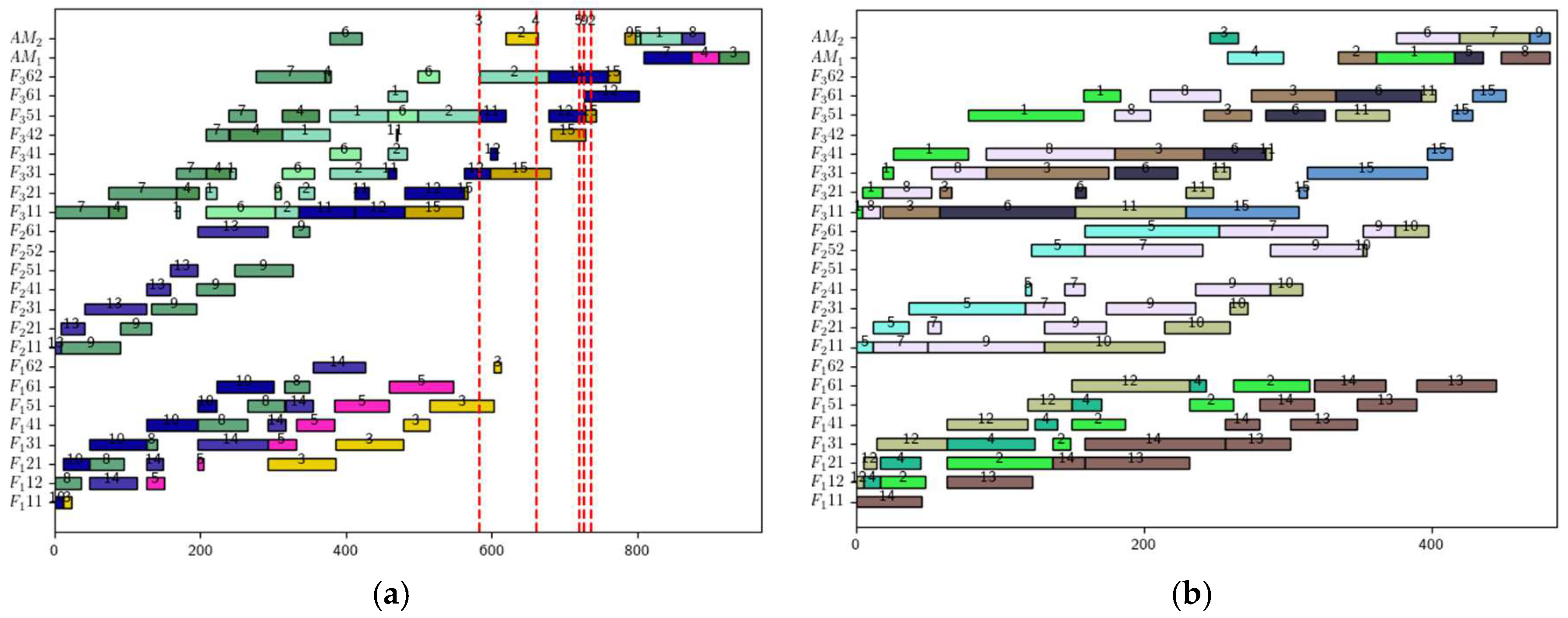
The mathematical model has been verified and validated through the Gurobi solver. To illustrate this issue with a simple case, consider the following parameters: t = 10, n = 16, f = 2, and w = 2. Each operation can be carried out on 1 to 2 parallel machines. Figure 2 shows the Gantt charts for two different schedules. In Figure 2a, the schedule is generated without blocking constraints. While in Figure 2b, the same schedule is executed considering the blocking constraints. It is evident that the schedule with the blocking constraint results in a larger time span and a longer system idle time. Therefore, the optimal solution for a mixed-flow workshop may not remain optimal when the blocking constraint is taken into account.

4. Symmetry Analysis of Q-Learning Reinforced NSGA-II

4.1. Symmetric Solution Representation

The solution space is partitioned into four symmetric components: jobs sequence S J , jobs assignment M J , assembly sequence S P and assembly assignment M P . This decomposition establishes stage-wise symmetry between processing and assembly operations, enabling parallel optimization of manufacturing stages and consistent constraint handling across stages.
The approach prioritizes minimizing processing time, initially computing the average processing time for each job across all factories. Subsequently, the product’s overall job processing time is prioritized to obtain the sorted order of product parts. The next step involves distributing tasks to factories according to which can complete waiting tasks the fastest. Within each factory, machines are assigned based on which can finish the current operation the soonest, leading to the initial assignment of machines for the first phase. The job sequence SJ is constructed from t part sequences ShJ. The part sequences ShJ and product sequence π are determined first, followed by connecting the t part sequences according to π.
For example, if a problem contains three products and nine jobs, and its subsequences are, respectively, S1J = [8, 6, 1, 9], S2J = [3, 4], S3J = [2, 5, 7], π = [3, 2, 1], then the complete job sequence is SJ = [2, 5, 7, 3, 4, 8, 6, 19]. It is crucial to emphasize that the job assignment to factory machines and the allocation of products to assembly machines may exhibit variability, even when utilizing the same S J and S P within the problem.

4.1.1. Subsequence Initialization for Jobs

Subsequences for ShJ are obtained by the following steps:
  • Set i = 1;
  • Calculate the average processing time of operation Oji in available machines of factory Fg as p j i g = k = M g , i 1 + 1 M g i p j k / K i g ;
  • Compute the average processing time of Oji across all factories as p j i = g = 1 f p j k g / f ;
  • Let i = i + 1. If i = m, proceed to the next step; otherwise, return to Step 2;
  • Compute the total processing time of job Jj with p j = i = 1 m p j i .
Subsequently, the jobs for Ph are arranged in ascending order by the value of pj, resulting in the sequence of parts ShJ.
Then the products are sorted according to the expected urgency, which can be evaluated with E U h = d h j = 1 n p j y j h . Finally, π is obtained by sorting d h in ascending order, resulting in S J = h = 1 t S h J .

4.1.2. Jobs Assignment to the Target Factory and Machines

Taking into account the constraint (6), which stipulates that each job can arrive at only one factory. Once the target factory is determined by the target machine for the first operation, the target machine for the remaining operations of each job can be selected according to the heuristic rule.
Specifically, let the current available time of a machine in factory Fg for the first operation be Tgk, where k = M g , 0 + 1 , , M g , 1 .
Then the target machine and factory are determined by minimizing the expression in Equation (20):
g * , k * = arg m i n g = 1 , , f ; k = M g , 0 + 1 , , M g , 1 ( T g k + i = 1 m p j i g )
Subsequently, the remaining job operations are processed in the target factory Fg. The target machine is selected based on Equation (21), where Tgk is the current available time of the machine in factory g for the ith operation. Variable Xjk = 1 is then satisfied for j = 1, …, n.
k * = arg m i n k = M g * , 0 + 1 ,     , M g * , 1 ( T g * k + i = 1 m p j k )

4.1.3. Products Sequencing and Allocation

After the jobs are assigned, the completion time Cji (for i = 1, …, m) of each job in factory Fg can be determined. Additionally, the expected lead time of each product is calculated using Equation (22). The sequence of products in the assembly stage is obtained by sorting E h in non-descending order.
E h = d h m a x j = 1 , , n { y j h C j m + a = 1 w r g a j / w }
To minimize the maximum tardiness, the assembly sequence is determined using Equations (23) and (24). Here, Ta represents the current available time of assembly machine a, Cjm is the completion time of job j in the processing stage, and rgaj is the transportation time of job j from its optimal factory g to assembly machine a. The variable Yha = 1 is then confirmed.
E h a = j = 1 n y j h ( C j m + r g a j )
a * = arg m i n a = 1 , , w ( max T a ,   E h a + q h a )

4.2. Mechanism and Four-Tuple in Reinforcement-Learning-Enhanced NSGA-II

The NSGA-II effectively handles two-objective conflicts by balancing them through nondominated sorting and crowding distance while maintaining population diversity.
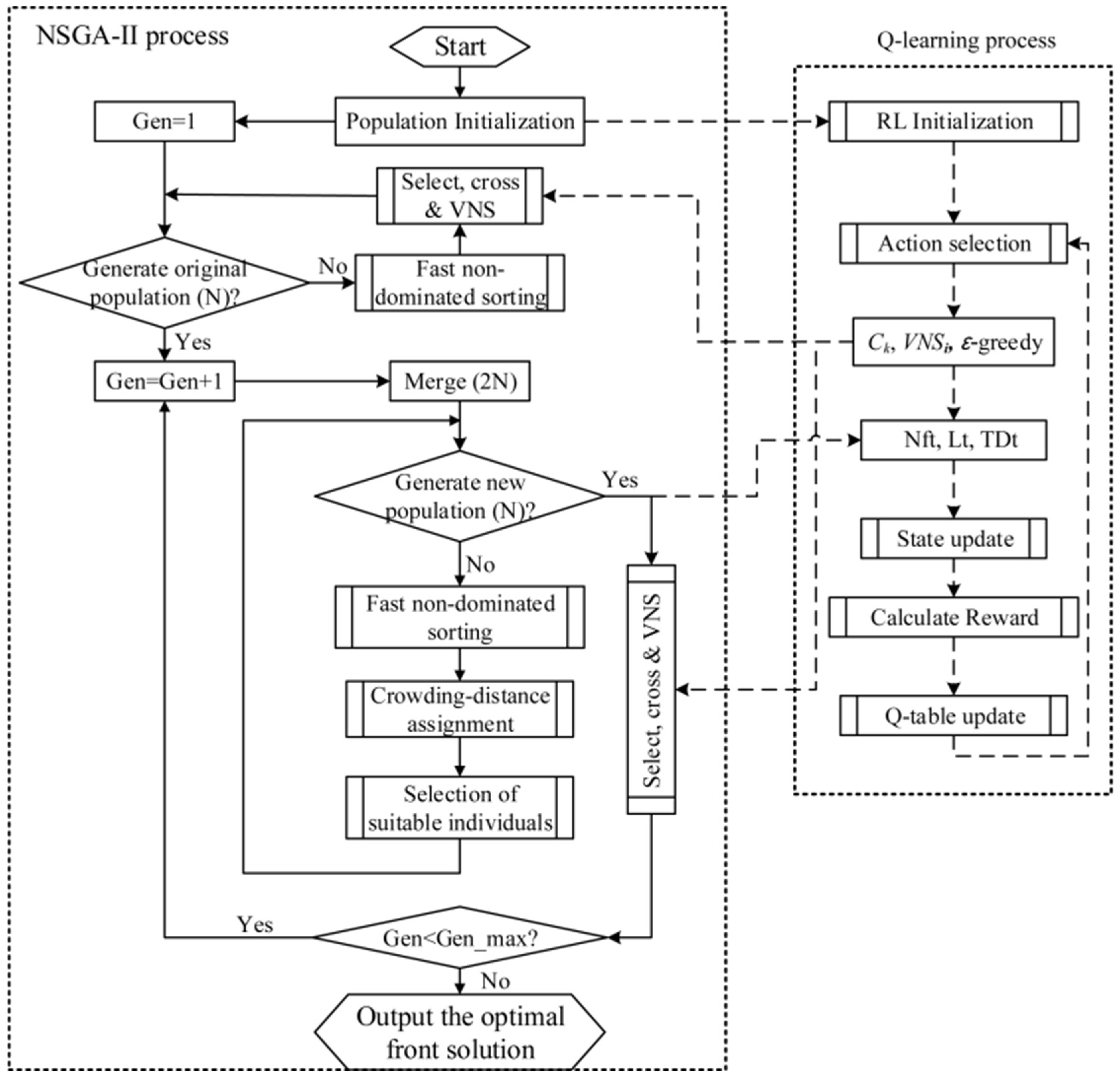
However, the decision-making process for complex problems can sometimes lead to local optima. To address this challenge, recent years have witnessed the integration of well-designed search methods to further enhance solutions [23,33,34,35,36]. In pursuit of this goal, we propose a QNSGA to expedite the optimization process, as shown in Figure 3.
RL algorithms excel in maximizing cumulative rewards through sequential actions in complex environments [37,38,39,40].
Q-learning is a classical model-free RL algorithm designed for value-based learning within a Markov Decision Process. Both Q-learning and SARSA continuously optimize the Q-value function using the Bellman equation, as shown in (25) and (26). The key distinction lies in their update methods: Q-learning, being bold and greedy, is indifferent to pitfalls, and SARSA adopts a more conservative approach, making it sensitive to errors and cautious. Q-learning is defined by a four-tuple (S, A, R, P), where S represents the state space capturing the agent’s schedule in the problem, A denotes the action space encompassing all possible selections when a state is reached, R reflects the reward function evaluating the effectiveness of an action in a given state, and P indicates the state transition probability function from one state to the next when an action is taken.
Q s t ,   a t   1 α   Q s t ,   a t + α   ( r t + γ   m a x a Q ( s t ,   a ) )
Q s t ,   a t   1 α   Q s t ,   a t + α   ( r t + γ   Q ( s ,   a ) )
Here, α represents the learning rate of the agent, γ is the discount factor, r t denotes the immediate reward from the system by acting a t in state s t , and m a x a Q ( s t , a ) is the largest Q-value among all actions at state s t .
The agent makes decisions based on optimal actions derived from the current Q-values in the Q-table. Initially, all Q-values are initialized to zero and updated as the agent learns from its experiences. By incorporating feedback from the exploration environment, the agent leverages its acquired knowledge to explore better alternatives. The ultimate objective is to achieve the best Q-table, leading to the most effective decision sequence or solution for the problem. The process of optimizing the Q-table involves striking a balance between exploration and exploitation, making the choice of strategy crucial. The ϵ -greedy strategy is a common approach to updating the Q-table. Under this strategy, the agent randomly selects an action a if a random value is less than ϵ . Otherwise, it selects the action a = a r g m a x a Q ( s t , a ) with the highest Q-value.
The Q-learning process is used to improve NSGA-II (QNSGA), and the components of the four-tuple are associated with algorithm parameters and strategies, as discussed in previous work [41], which was proposed for single-objective problems. Specifically, s t represents the population evaluation in the tth iteration. The quality of a ‘population’ can be assessed through changes in non-dominated solutions, crowding distances of each non-dominated front, and fitness improvements in the best solutions. a t denotes the selected update method, r t quantifies the degree of improvement produced by the selected action for the population, and P can be a random transition probability due to random search strategies.

4.3. States Construction in Q-Learning

In the QNSGA, the initial population is generated with random solutions and subsequently updated using one or more search strategies. Each population is evaluated across three dimensions, each compared with the previous one. The first dimension of population quality is the relative count of advantageous objectives compared with the last population, denoted as N f t . Suppose that the ith best solution fitness in the tth population is D i t . In dual-objective problems, N f t = 2 if D i t > D i , t 1 i .
The second dimension L t assesses the number of non-dominated solutions. If the number of nondominated solutions l t is larger than the former population l t 1 , the indicator L t is one, otherwise, it is zero.
The third dimension T D t is the relatively large distance of the non-dominated front. If the total crowding distance is larger than the former population, T D t is 1, otherwise, it is 0. Consequently, the total number of possible states is 12, S = { S 1 , , S 12 } , as summarized in Table 1.
12 states are defined by symmetric triple evaluation with three dimensions:
Nft: Dominance improvement (symmetric scaling);
Lt: Non-dominated solution count (cardinal symmetry);
TDt: Crowding distance (diversity metric symmetry).

4.4. Actions Symmetry Construction in QNSGA

In QNSGA, actions are comprised of combinations of searching and preservation strategies to explore and update the population. Each solution consists of four parts: job sequence, job assignment to machines, product sequence, and product assignment to assembly machines. Different searching methods are developed for various scenarios. This section introduces two metaheuristics of VNS for solution evolution and two crossover operators for solution interaction. It is noteworthy that each update in the processing stage triggers the corresponding update in the assembly stage based on heuristic methods. However, the update in the assembly stage does not affect the processing stage.
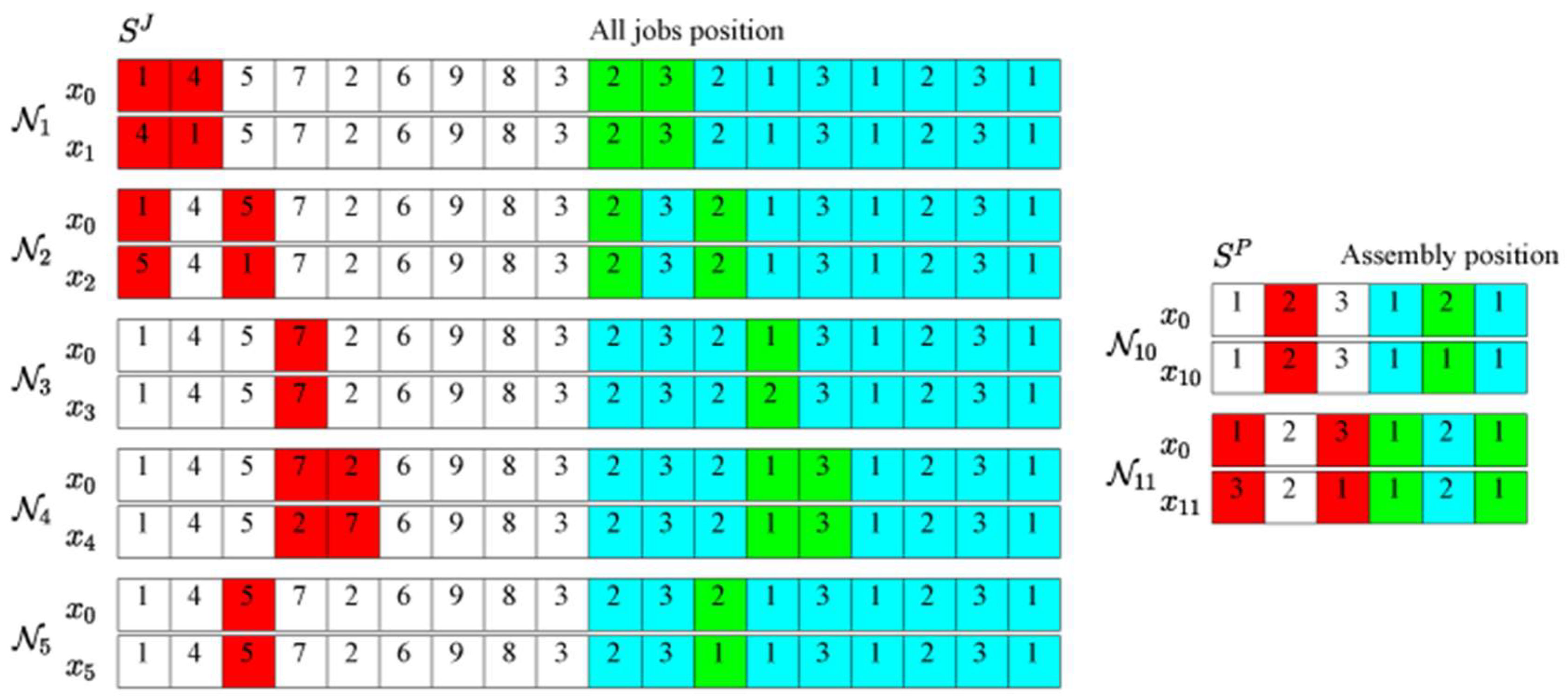
As depicted in Figure 4, N 1 attempts to exchange two jobs y j h = y j h belonging to a product but assigned to different factories X j k X j k ( k ) . The distinction between N 2 and N 1 is that the assigned factories of the two jobs are the same. Moving on to N 3 , the target factory assigned to a job is randomly changed. N 4 involves selecting two different jobs of a product and reversing their order. In N 5 , the factory with the most jobs is identified, and one job is selected and assigned to the shortest factory. N 6 is similar to N 5 , but it transfers a job from the factory with the largest completion time to the one with the least completion time.
Continuing with the longest factory, two different jobs are selected and swapped in the sequence with N 7 . In N 8 , the processing machine with the most jobs are selected, and two jobs are swapped within it. In N 9 , part sequences of S 1 J and S 2 J are exchanged in the total sequence.
The assembly stage is also updated by changing the assembly machine of a product using N 10 ; then one of the products in the most popular assembly machine is transferred to the one with the minimum load by N 11 .
With any of the 11 neighborhood structures mentioned above, each solution can be partially updated independently. To balance the updating of the processing stage and assembly stage, two VNS methods, V N S 1 and V N S 2 , are designed by combining neighborhood structures N 1 to N 11 . V N S 1 operates on a solution x 0 with the following steps:
  • Set b = 1 and e   = 0;
  • Generate a solution x b with a random search N b based on x 0 ;
  • If x b is superior to x 0 , update x 0   =   x b , set e   = 1 , and proceed to Step 5; otherwise, increment b and go to Step 4;
  • If b = 11, proceed to Step 5; otherwise, return to Step 2;
  • Output the solution x 0 and terminate the search.
As the eleven neighborhoods do not have prioritization during the search process, V N S 2 reorders the eleven neighborhood structures and is executed similarly to V N S 1 .
Neighborhood structures exhibit structural symmetry:
  • Intra-factory symmetry: N2 (job swap in same factory) and N8 (job swap on same machine) share identical permutation logic;
  • Cross-stage symmetry: N5 (job transfer between factories) and N11 (product transfer between assembly machines) both implement load-balancing heuristics;
  • Unified procedure: Both stages use identical VNS update mechanisms (VNS1, VNS2).
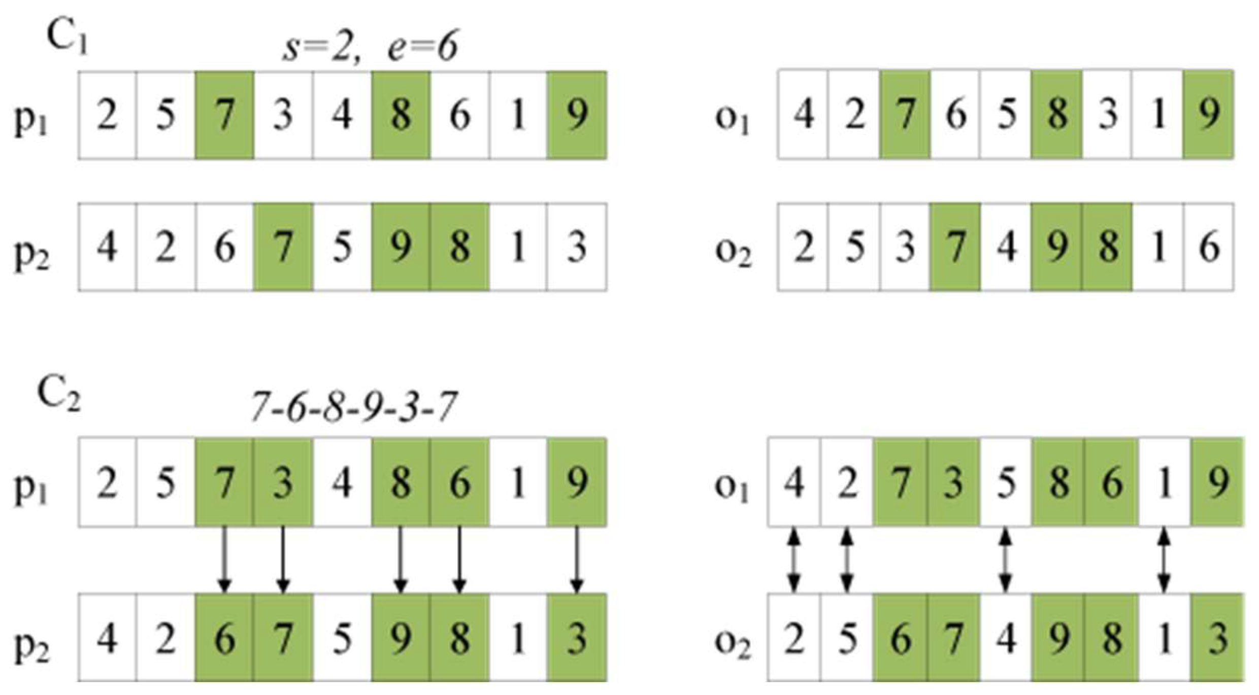
The VNS methods mentioned earlier operate on the solution itself. In contrast, two crossover operators, C 1 and C 2 , are designed to evolve the job sequence (Figure 5). The process of C 1 with solutions p 1 and p 2 involves randomly generating two numbers, s and e (s < e), selecting jobs between s and e from both p 1 and p 2 , then swapping the order of jobs in p 1 and p 2 , keeping the others unchanged. C 2 operates by finding a cycle of jobs and exchanges the jobs outside the cycle. For example, assume that the random job in p 1 is 7, and the job in the same position of p 2 is 6, then the position of the 6 in p 1 is 7, the job in position 7 pf p 2 is 8. The procedure continues until a cycle 7-6-8-9-3-7 is obtained. Jobs in the cycle remain while jobs outside the cycle exchange the position in two positions.
Both operators preserve permutation symmetry:
C1: Positional swap maintaining sequence validity
C2: Cycle-based exchange preserving topological order.
In addition to the updating methods, the preservation strategy is also a crucial part of updating the population actions. For QNSGA with an adaptive strategy, aggressive exploration is encouraged in the early stages, followed by conservative exploitation of the found experience or solution. The consequence of this phenomenon is the trade-off between exploration and exploitation, thus creating an equilibrium. Consequently, both the ϵ -greedy strategy and the greedy strategy are integrated into the action set.
Eight actions A = [ A 1 , , A ( 8 ) ] are established, as listed in Table 2, where A c c 1 is the ϵ -greedy acceptance rule, and A c c 2 is the greedy acceptance rule.
A 1 works as follows.
  • Randomly select two solutions x 1 and x 2 from different Pareto fronts, where x 1 dominates x 2 .
  • Generate two offspring solutions x g 1 and x g 2 with crossover C 1 and compare them with x 1 .
  • If the dominated one of x g 1 and x g 2 can dominate x 1 , substitute x 1 with the better solution; otherwise, let r = rand(0,1), if r   > ϵ , substitute x 1 with the better solution; otherwise, update x 1 with V N S 1 based on the ϵ -greedy acceptance rule.

4.5. Reward Function Determination

A reward is generated when a superior population is produced. In Section 4.4, twelve states are proposed based on possible changes in a population. In the standard NSGA-II, if the best solution of a population dominates that of another population, then it is considered better and should be encouraged. Consequently, State 9 is valued more than State 1. On the contrary, we prioritize state 5 over state 1 to promote the exploration of solutions. Additionally, considering the number of non-dominated solutions, more substantial crowding distance may lead to better solutions. Therefore, State 3 is assigned greater importance than State 2. The most favorable state is State 12, indicating the generation of a dominant solution. In summary, the reward function is defined as r t = θ s t θ s t 1 , where θst is the labeled state of st in Table 1.

4.6. Procedure of QNSGA

The algorithm’s parameters consist of the population size (N), the maximum execution time (TM), the crossover probability (pc), and the acceptance probability for suboptimal solutions (ϵ). The flowchart of the QNSGA algorithm is presented in Figure 3.
Initially, a population comprising N solutions is generated randomly. Following this, the population undergoes fast non-dominated sorting, yielding a set of non-dominated front solutions, denoted as NF = {F1, …, Flt}, where lt (≤N) is the count of non dominated solutions in the tth generation. To create a new population, solutions from P \NF are selected to execute the action at = (Ck, VNSi, Accp). The procedure is outlined in Algorithm 1. Conversely, in study [20], batched transportation constraints yield fragmented feasible solutions ill-suited for reinforcement learning.
Upon obtaining a new population P , the next step involves merging P and P if the maximum generation count is not reached. Simultaneously, the quality of P is evaluated, updating the state st. Subsequently, the reward generated by the state transition and at is calculated, refreshing the Q-table. The procedure to update the Q table with twelve states and eight actions is determined by Algorithm 2. In this algorithm, the ϵ-greedy policy is taken to select the target action, while the ϵ-greedy acceptance rule in the designed actions Ai (i = 1, …, 8) in Section 4.5 is utilized to determine the updated solution.
Algorithm 1: Generate a new population of size N.
Require: Original population P , selected action at = (Ck, VNSi, Accp)
Ensure: A new population P
j l t ,   P N F
while jN do
  Select a solution x r randomly from P \NF
  Select an elite solution x g randomly from NF
  Cross xr and xg with Ck
  if xr dominates x g then
    Append xr to P
    j++
  else
    Randomly generate r ⇐ rand (0, 1)
    if r is acceptable with Accp then
      Append xr to set  P
    else
      Search the neighborhood solution of xr with VNSi
      if xr is acceptable with Accp then
        Append xr to set P
        j ++
      end if
    end if
  end if
end while
Algorithm 2: QNSGA for the problem
Require: Problem environment set, learning rate α, discount factor γ, exploration rate ϵ, maximum running time TM Initialize the population P .
Perform non-dominated sorting and compute the crowding distance.
Initialize the Q-table, current time, and state s based on the population P of the initial generation.
Select an action a from state s by applying the ϵ-greedy policy informed by the Q-table.
while t < TM do
  Take action a to generate a new population P , observe the new state s′ and reward
   Choose action a′ from s′ using the ϵ-greedy policy derived from the Q-table
  Perform non-dominated sorting and compute the crowding distance.
  Update the Q-value for the current state-action pair using Equation (25)
  Update current state and action: s ← s′, a ← a
end while

5. Experimental Evaluation and Industrial Validation

This section systematically assesses the performance of the proposed QNSGA when applied to the three-stage DAPFSP. The evaluation is conducted through an extensive suite of numerical experiments, aimed at quantifying the algorithm’s efficiency and efficacy. Initially, the QNSGA undergoes a meticulous calibration process to fine-tune its parameters. Subsequently, its performance is juxtaposed with that of established multi-objective optimization algorithms (including Gurobi 11.0.0).
All computational experiments in this study were implemented in Python 3.10 for its robustness and versatility in scientific computing. The experiments were conducted on an Intel Core i7-8700H processor, 16 GB of RAM, and the Windows 11 operating system, ensuring a consistent and powerful computational environment for algorithmic comparison.

5.1. Experimental Methodology

Random instances are generated based on the problem-specific parameters outlined in Table 3. These instances vary according to the number of products (t), number of operations (m), number of factories (f), number of jobs per product (|Ph|), number of parallel machines (Kil), and number of assembly machines. Two separate experimental sets are designed to independently validate the proposed methodologies. For the small-scale cases, the number of parallel machines is selected from the set {1, 2, 3}, whereas for the large-scale cases, it is chosen from {1, 2, 3, 4, 5}. The number of parallel assembly machines is defined as ⌈t/2⌉. Machine operation times are randomly generated within the interval [1, 99], consistent with common practices in related scheduling research [15,42]. Assembly times for each product are dependent on the number of assigned jobs and are sampled from a specified interval. Transportation times between factories and assembly facilities are randomly drawn from the interval [1, 49], as reported in prior studies [3]. Due date times are established with reference to existing literature [43].
In total, 108 parameter combinations are constructed, with ten instances generated for each combination, resulting in a total of 1080 instances. The experiments utilize uniform termination criteria and consistent encoding and decoding procedures across all algorithms employed.
Three distinct performance metrics are employed to assess the effectiveness of the algorithms [4,14,44]: (1) Spread (Δ), which measures the uniformity of the distribution within the Pareto solution set; (2) Generational Distance (GD), which evaluates the convergence behavior of the algorithms; and (3) Inverse Generational Distance (IGD), a composite metric that concurrently captures both uniformity and convergence. Following the execution of each algorithm, the resulting non-dominated solution sets are meticulously documented and subsequently amalgamated with those generated by other algorithms. Following the conclusion of all experimental runs, a comprehensive ideal non-dominated solution set is to be established.
The experimental setup is illustrated in Figure 6. The parameters of the QNSGA algorithm are optimized in accordance with the principles of Design of Experiments (DOE) and Analysis of Variance (ANOVA), methodologies frequently utilized in scheduling research for algorithm calibration [7,38]. In order to validate the accuracy of the proposed mathematical model, it was solved using the Gurobi 11.0.0 solver across multiple problem instances. Furthermore, a comparative analysis was conducted between QNSGA and its variants to ascertain the efficacy of its core mechanisms. Subsequent to the comparative evaluation, statistical differences among the various methods were analyzed using ANOVA. In conclusion, the proposed approaches were applied to a pharmaceutical manufacturing case study.

5.2. Calibration of Algorithmic Parameters

The effectiveness of the QNSGA algorithm depends critically on the precise adjustment of four key parameters: the initial population size (N), the greediness coefficient ( ϵ ), the learning rate ( α ), and the discount factor ( γ ). The optimization of these parameters is conducted through a systematic approach employing Analysis of Variance (ANOVA) in conjunction with Design of Experiments (DOE) techniques. ANOVA serves as a robust statistical tool for discerning significant variances among group means, a technique instrumental in parameter optimization [45]. DOE, conversely, provides a structured framework for experimental planning, enabling a comprehensive assessment of how individual factors influence the outcome variable [46].
Preliminary empirical data have been utilized to delineate potential parameter ranges: N = {10,20,30,50}, ϵ = { 0.01 , 0.1 , 0.15 , 0.2 } , α = { 0.1,0.15 , 0.2 , 0.3 } , γ = { 0.8,0.85,0.9,0.99 } . To mitigate the risk of overfitting and to ensure the generalizability of the model, 16 distinct problem instances have been artificially constructed for the calibration process. These instances encapsulate a diverse spectrum of scenarios, defined by varying combinations of t ∈ {10, 20}, m ∈ {3, 5}, f ∈ {2, 5}, |Ph|   {4,6}, with additional parameters detailed in Table 3. For each combination, five unique instances are crafted, and each is subjected to ten independent runs. The computational budget for each run is capped at Tmax = ln (n) × f × m CPU seconds, a criterion that has been observed to yield near-optimal solutions for smaller instances when compared against the Gurobi solver.
The response metric is articulated as ρ i = | P F i P F * | | P F * | , for the ratio of nondominated solutions to the cardinality of the true Pareto front. A larger ρi indicates a better combination of algorithm parameters. The empirical results, as articulated in Table 4, reveal that the optimal parameter set is configuration 6, with corresponding p-values that are uniformly below the threshold of 0.05, denoting a statistically significant parameter impact on the QNSGA’s performance. Figure 7 displays a mean response plot accompanied by 95% Least Significant Difference (LSD) intervals, providing visual confirmation of the optimality of the parameter set: N = 20, ϵ = 0.1 , α = 0.15 and γ = 0.99 .

5.3. Assessment of the Mathematical Model

The efficacy of the mathematical model is rigorously examined utilizing the Gurobi mathematical programming solver, adhering to the methodological frameworks established in pertinent literature [37]. We employ small-scale instances for this validation exercise, allocating a maximum solving duration of 2100 s to Gurobi, whereas the runtime for QNSGA is governed by Tmax = t × f × m CPU seconds.
Since the Gurobi solver does not inherently support bi-objective optimization models, we effectively reformulate the problem into an equivalent single-objective framework. Let the objectives of the optimal solution derived from six heuristics be denoted as f10 and f20. The composite objective function is then articulated as f = f 1 / f 1 0 + f 2 / f 2 0 , where equal weighting is applied to both objectives, underscoring their equivalence in significance and the proportional reduction observed in our experiments. This methodological adaptation enables us to harness Gurobi’s computational prowess while adhering to the unique constraints inherent in our model. The Relative Percentage Deviation (RPD) serves as the evaluative metric, operationalized through Equation (27).
R P D = f i f b e s t f b e s t 100 %
where f i is the ith objective is yielded by a given algorithm for a specified instance, while f b e s t represents the makespan or maximum tardiness of the optimal solution identified across all compared methodologies, inclusive of the MILP solver.
Table 5 presents a comparative analysis of the computational outcomes and the average execution time for both the MILP solver and QNSGA, delineating the mean and standard deviation (STD) of RPD. The results presented in Table 5 indicate that the MILP solver attains the optimal solution within relatively short computational times for both objectives solely in the case where t = 3. For t = 5, while the model identifies the optimal solution for maximum tardiness, the computational expense escalates, nearing 1404.29 s. The model encounters insurmountable challenges in optimally resolving the majority of instances with t = 8, with computational times reaching the threshold of 2100 s. QNSGA, while slightly outperformed by the MILP solver for t = 3 and 5 on the second objective, demonstrates superiority over the Gurobi solver for t = 8 on the first objective. As the problem scale escalates, QNSGA consistently yields more satisfactory outcomes compared to the MILP solver. More notably, QNSGA’s computational demands are significantly lower than those of the MILP solver. Concurrently, QNSGA exhibits a lower standard deviation across the majority of instances, indicative of its enhanced stability. Consequently, QNSGA is capable of generating promising solutions for small-scale instances within a compressed time frame, whereas the MILP solver is deemed more suitable for instances of a smaller scale.

5.4. Effectiveness of Eight Actions

This section delves into the efficacy of the eight distinct actions within the QNSGA, as enumerated in Table 2. To assess these actions, we introduce eight specialized variants of QNSGA, denoted as V i , each exclusively incorporating a single action a i . A rigorous experimental framework is employed, with each variant subjected to ten iterations on large-scale problem instances. The computational budget for these experiments is capped by a maximum running time, calculated as T m a x = t × l n ( f × m × | P h | ) CPU seconds, ensuring a consistent evaluation baseline.
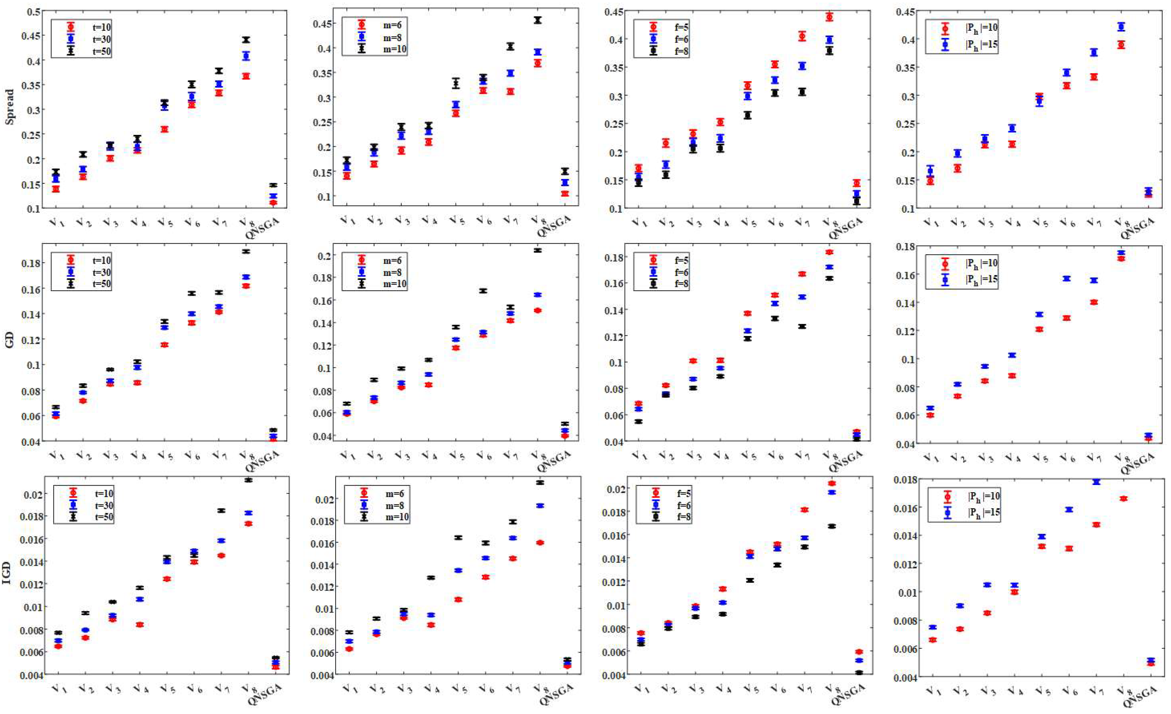
Table 6 synthesizes a comparative analysis between the original QNSGA and its eight variants across large-scale instances, while Figure 8 graphically represents the average performance metrics per instance. Employing Equation (22), the optimal performance metric is identified by benchmarking against all compared algorithms.
The data in Table 6 consistently indicate that QNSGA outperforms its variants in identifying dominant solutions across three key metrics. Notably, the variant V 1 excels, whereas V 8 lags behind. The performance metrics escalate with an increase in parameters t, m, and |Ph|, whereas an increase in the factory parameter f is associated with a decline in metric values. This inverse relationship suggests that the problem’s complexity diminishes with a higher number of factories, potentially due to increased flexibility in scheduling. The variants, constructed from three pairs of operators, reveal the intrinsic differences between the searching operators. Figure 8 presents the 95% interval Least Significant Difference (LSD) among the algorithms, highlighting an ascending trend in performance metrics for the variants, with the exception of QNSGA. The operators forming V 1 emerge as the most efficacious.
Further validation is provided by the Friedman test in Table 7, applied to the nine algorithms, which confirms significant performance differences among them at a threshold of 0.05. This prompts a deeper investigation into the frequency of operator application. Figure 9, presenting boxplots of operator frequency, underscores the superiority of operator C1 over C2, Acc1 over Acc2, and the ϵ -greedy policy over a purely greedy approach.
Additionally, we meticulously recorded the application frequency of each operator throughout the QNSGA’s iterative process. The findings indicate that the VNS operator VNS1 contributes most significantly, followed by the ϵ -greedy policy, crossover C 1 and the remaining trio of operators.

5.5. Comparison with State-of-the-Art Algorithms

This section provides a comparative analysis of the proposed algorithm in relation to several state-of-the-art methods developed for similar problems. The algorithms selected for this comparison are MOPSO [22], QSFL [31], RLABC [41], CWWORL [40], and CMAF [47]. Additionally, to benchmark the performance of our Q-learning integrated NSGA-II (QNSGA), we have adapted the SARSA algorithm into NSGA-II, denoted as SNSGA. Given that these selected algorithms were not originally tailored for the specific problem addressed in this paper, we retained their core algorithmic frameworks while modifying other components, such as encoding, decoding, crossover, mutation, and neighborhood structures, to align with the requirements of our study.
Employing the established metrics of Δ, GD, and IGD, the comparative results of the metaheuristic algorithms are displayed in Table 8 and illustrated in Figure 10. The findings indicate that both SNSGA and QNSGA generally outperform the other five algorithms across various instances. Notably, SNSGA surpasses QNSGA in certain scenarios where the problem scale is modest; however, QNSGA demonstrates a marked dominance over SNSGA in the majority of cases, particularly as the problem scale escalates. The LSD intervals depicted in Figure 10 underscore significant performance differences among the algorithms, which are especially pronounced with large-scale problems. Furthermore, the metric values are positively influenced by an increase in parameters t, m, and |Ph|, and inversely affected by an increase in the factory parameter f.
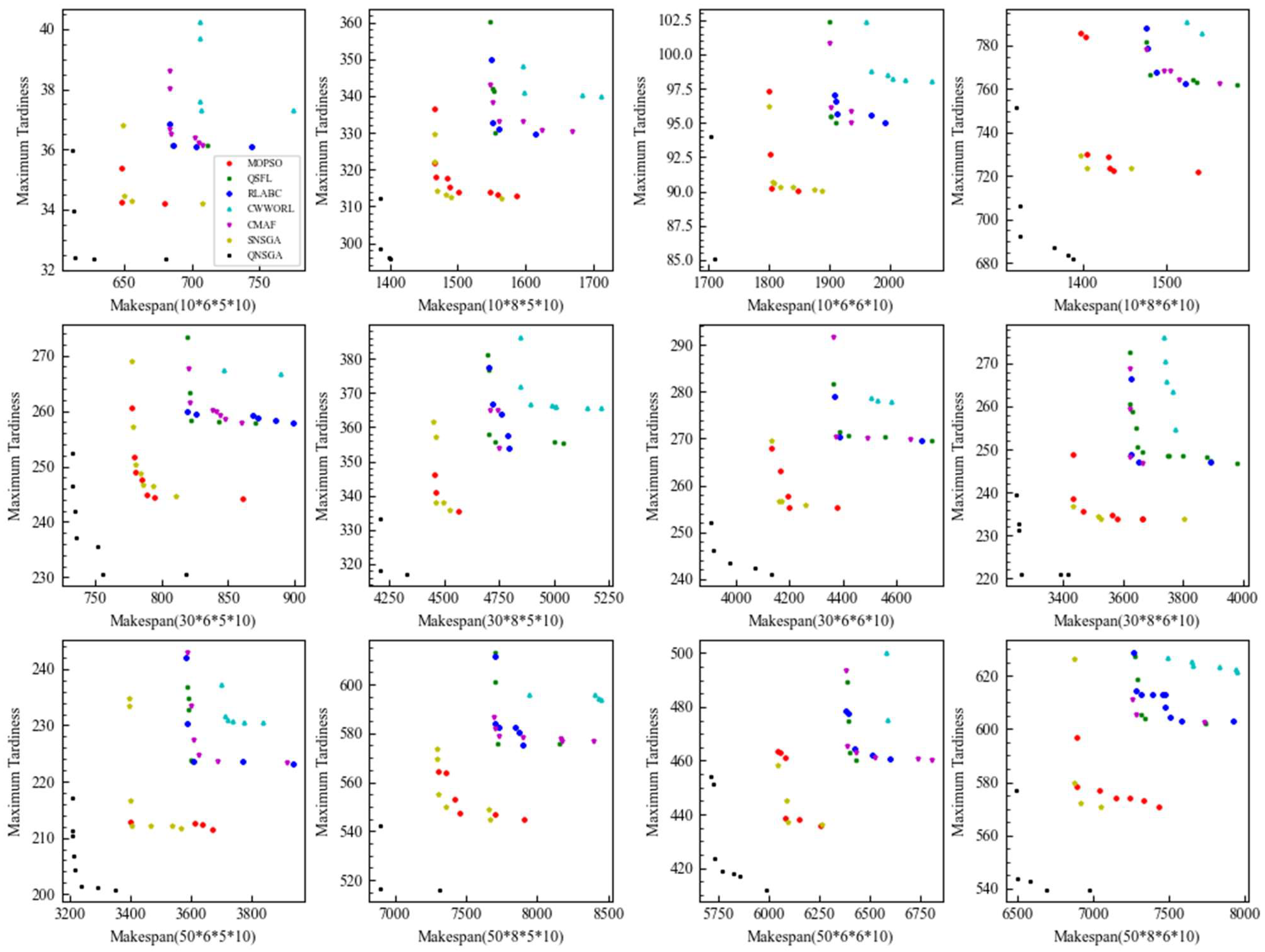
To statistically validate the comparative results, the Friedman test is applied to the three metrics obtained from the seven metaheuristic algorithms. The results, as documented in Table 9, confirm the existence of statistically significant differences between the algorithms. Additionally, the Pareto front solutions from twelve distinct cases are visualized in Figure 11, where the non-dominated solutions of the seven algorithms are juxtaposed. The visualization clearly demonstrates that QNSGA consistently identifies superior dominant solutions.

5.6. Industrial Case Study: Wind Turbine Manufacturing Application

This section presents an industrial case study within the wind turbine manufacturing sector, focusing on the application of the DHFSTFA model and the QNSGA algorithm to a real-world problem [48]. The case involves the assembly of nine distinct products, each requiring a sequence of operations including material intake, identification engraving, milling, polishing, cleaning, and final inspection. The workshop is equipped with multiple machines capable of performing identical operations, such as milling machines X52K, HCN6800-II, and BV100, among others, which underscores the complexity and variability inherent in the scheduling process.
The objective of this case study is to optimize the scheduling order for each job to minimize the makespan and reduce the maximum tardiness. Utilizing seven metaheuristic algorithms, including the proposed QNSGA, the case is solved, and Pareto front solutions are obtained. Figure 12 illustrates the mean objective values of each set of non-dominated solutions for each algorithm across iterations. It is evident that QNSGA can identify superior solutions more rapidly and converge to the non-dominated solution set with greater efficiency.
A comparative analysis within Figure 13 examines one of the initial solutions and the final solution yielded by QNSGA. The makespan is notably reduced by 49.36% (from 952.65 to 482.43), and the maximum tardiness is eliminated (from 369.36 to 0), which is a testament to the high search efficiency of QNSGA. These results are particularly significant in the context of wind turbine manufacturing, where operational efficiency and timeliness are critical for meeting production goals and ensuring customer satisfaction.
The industrial case study demonstrates the practical applicability of the QNSGA algorithm in a complex manufacturing environment. The significant improvements in makespan and tardiness highlight the potential of QNSGA for optimizing scheduling in the wind turbine industry and other sectors with similar logistical challenges. The case study serves as a validation of the QNSGA’s robustness and effectiveness in real-world scenarios, providing a promising solution for industry professionals seeking to enhance their production scheduling strategies.

6. Conclusions and Future Work

This study introduces a novel three-stage Distributed Heterogeneous Hybrid Flowshop Scheduling with Transportation and Flexible Assembly (DHFSTFA) model, tailored for the wind turbine manufacturing process. The model addresses the intricate logistics of transporting individual workpieces from various manufacturing stages to an assembly station, where final assembly is conducted. Given the complexity of this scheduling paradigm, we have devised a Q-learning augmented Non-dominated Sorting Genetic Algorithm II (QNSGA). Our approach integrates two distinct crossover operators, two variable neighborhood search operators, and an ε-greedy policy to enhance the exploration and exploitation balance within the solution space.
Through rigorous experimentation, we have substantiated the efficacy of our proposed algorithm. Initially, a Taguchi experimental design was employed to identify the optimal parameters of the algorithm. Subsequent small-scale experiments, leveraging the Gurobi solver, validated the mathematical model’s effectiveness, demonstrating that QNSGA achieves performance comparable to Gurobi within a significantly shorter time frame. Ablation studies on the eight actions within QNSGA confirmed their individual effectiveness and established significant differences among them, thereby pinpointing the most effective actions.
Furthermore, we conducted comparative experiments with other algorithms, focusing on the optimization of makespan and maximum tardiness. The results of these comparisons corroborate the superior performance of QNSGA. After each comparative trial, Least Significant Difference (LSD) tests and Friedman tests were conducted. These statistical methodologies provided auxiliary evidence, affirming the superiority of QNSGA.
In future research, we aim to expand our exploration of diverse distributed scheduling challenges and their applicability in real-world scenarios, while simultaneously enhancing the design of RL algorithms to achieve greater efficiency. Additionally, we plan to broaden the scope of our investigations to address the multifaceted demands of contemporary production environments, thereby contributing to the advancement of scheduling methodologies in industrial settings.

Author Contributions

Z.S.: methodology, conceptualization, validation, writing—original draft, H.C.: funding acquisition, writing—review and editing. F.Y.: writing—review and editing. X.D.: writing—review and editing. H.H.: writing—review and editing. J.Z.: writing—original draft, terms, data curation. Q.Y.: methodology, conceptualization, validation, writing—original draft, term, data curation. All authors have read and agreed to the published version of the manuscript.

Funding

This work is supported in part by the National Natural Science Foundation of China under Grant No. 52305533, the Major science and Technology Project of the Sichuan Province of China under No. 2022ZDZX0003, and the National Key Research and Development Program of China under Grant No. 2023YFB3307900.

Data Availability Statement

The original contributions presented in this study are included in the article. Further inquiries can be directed to the corresponding author.

Conflicts of Interest

Authors Zhiyuan Shi, Fuqian Yan, Xutao Deng, Jialei Zhang, and Qingwen Yin were employed by Dongfang Electric Academy of Science and Technology Co., Ltd. The remaining authors declare that the research was conducted in the absence of any commercial or financial relationships that could be construed as a potential conflict of interest. The funder was not involved in the study design, collection, analysis, interpretation of data, the writing of this article, or the decision to submit it for publication.

References

  1. Liu, C.G.; Yang, N.; Li, W.J.; Lian, J.; Evans, S.; Yin, Y. Training and assignment of multi-skilled workers for implementing seru production systems. Int. J. Adv. Manuf. Technol. 2013, 69, 937–959. [Google Scholar] [CrossRef]
  2. Zhang, G.; Xing, K.; Zhang, G.; He, Z. Memetic Algorithm with Meta-Lamarckian Learning and Simplex Search for Distributed Flexible Assembly Permutation Flowshop Scheduling Problem. IEEE Access 2020, 8, 96115–96128. [Google Scholar] [CrossRef]
  3. Hao, H.; Zhu, H.; Shen, L.; Zhen, G.; Chen, Z. Research on assembly scheduling problem with nested operations. Comput. Ind. Eng. 2023, 175, 108830. [Google Scholar] [CrossRef]
  4. Wu, X.L.; Liu, X.J.; Zhao, N. An improved differential evolution algorithm for solving a distributed assembly flexible job shop scheduling problem. Memetic Comput. 2019, 11, 335–355. [Google Scholar] [CrossRef]
  5. Dolgui, A.; Ivanov, D.; Sethi, S.P.; Sokolov, B. Scheduling in production, supply chain and Industry 4.0 systems by optimal control: Fundamentals, state-of-the-art and applications. Int. J. Prod. Res. 2019, 57, 411–432. [Google Scholar] [CrossRef]
  6. Zhang, Z.-Q.; Hu, R.; Qian, B.; Jin, H.-P.; Wang, L.; Yang, J.-B. A matrix cube-based estimation of distribution algorithm for the energy-efficient distributed assembly permutation flow-shop scheduling problem. Expert Syst. Appl. 2022, 194, 116484. [Google Scholar] [CrossRef]
  7. Hosseini, S.M.H. Distributed assembly permutation flow-shop scheduling problem with non-identical factories and considering budget constraints. Kybernetes 2022, 52, 2018–2044. [Google Scholar] [CrossRef]
  8. Zheng, J.; Wang, Y. A Hybrid Bat Algorithm for Solving the Three-Stage Distributed Assembly Permutation Flowshop Scheduling Problem. Appl. Sci. 2021, 11, 10102. [Google Scholar] [CrossRef]
  9. Yang, S.; Xu, Z. The distributed assembly permutation flowshop scheduling problem with flexible assembly and batch delivery. Int. J. Prod. Res. 2021, 59, 4053–4071. [Google Scholar] [CrossRef]
  10. Hatami, S.; Ruiz, R.; Andres-Romano, C. The Distributed Assembly Permutation Flowshop Scheduling Problem. Int. J. Prod. Res. 2013, 51, 5292–5308. [Google Scholar] [CrossRef]
  11. Hatami, S.; Ruiz García, R.; Romano, C.A. The Distributed Assembly Parallel Machine Scheduling Problem with eligibility constraints. Int. J. Prod. Manag. Eng. 2015, 3, 13–23. [Google Scholar] [CrossRef]
  12. Li, Z.; Qian, B.; Hu, R.; Zhang, C. Adaptive hybrid estimation of distribution algorithm for solving a certain kind of three-stage assembly flowshop scheduling problem. Comput. Integr. Manuf. Syst. 2015, 21, 1829–1845. [Google Scholar]
  13. Kim, M.-G.; Yu, J.-M.; Lee, D.-H. Scheduling algorithms for remanufacturing systems with parallel flow-shop-type reprocessing lines. Int. J. Prod. Res. 2015, 53, 1819–1831. [Google Scholar] [CrossRef]
  14. Huang, Y.-Y.; Pan, Q.-K.; Gao, L.; Miao, Z.-H.; Peng, C. A two-phase evolutionary algorithm for multi-objective distributed assembly permutation flowshop scheduling problem. Swarm Evol. Comput. 2022, 74, 101128. [Google Scholar] [CrossRef]
  15. Fu, Y.; Zhang, Z.; Liang, P.; Tian, G.; Zhang, C. Integrated remanufacturing scheduling of disassembly, reprocessing and reassembly considering energy efficiency and stochasticity through group teaching optimization and simulation approaches. Eng. Optim. 2024, 56, 2018–2039. [Google Scholar] [CrossRef]
  16. Maria Gonzalez-Neira, E.; Ferone, D.; Hatami, S.; Juan, A.A. A biased-randomized simheuristic for the distributed assembly permutation flowshop problem with stochastic processing times. Simul. Model. Pract. Theory 2017, 79, 23–36. [Google Scholar] [CrossRef]
  17. Jiang, N.-Y.; Yan, H.-S. Integrated optimization of production planning and scheduling in uncertain re-entrance environment for fixed-position assembly workshops. J. Intell. Fuzzy Syst. 2022, 42, 1705–1722. [Google Scholar] [CrossRef]
  18. Allahverdi, A.; Al-Anzi, F.S. Evolutionary heuristics and an algorithm for the two-stage assembly scheduling problem to minimize makespan with setup times. Int. J. Prod. Res. 2006, 44, 4713–4735. [Google Scholar] [CrossRef]
  19. Talens, C.; Fernandez-Viagas, V.; Perez-Gonzalez, P.; Framinan, J.M. New efficient constructive heuristics for the two-stage multi-machine assembly scheduling problem. Comput. Ind. Eng. 2020, 140, 106223. [Google Scholar] [CrossRef]
  20. Hao, H.; Zhu, H.; Luo, Y. A multi-objective Immune Balancing Algorithm for Distributed Heterogeneous Batching-integrated Assembly Hybrid Flowshop Scheduling. Expert Syst. Appl. 2025, 259, 125288. [Google Scholar] [CrossRef]
  21. Yuan, Y.; Xu, H. Multiobjective Flexible Job Shop Scheduling Using Memetic Algorithms. IEEE Trans. Autom. Sci. Eng. 2015, 12, 336–353. [Google Scholar] [CrossRef]
  22. Zhao, Y.; Wang, Y.; Tan, Y.; Zhang, J.; Yu, H. Dynamic Jobshop Scheduling Algorithm Based on Deep Q Network. IEEE Access 2021, 9, 122995–123011. [Google Scholar] [CrossRef]
  23. Zhu, C.; Sun, G.; Yang, K.; Huang, Y.; Cheng, D.; Zhao, Q.; Zhang, H.; Fang, X. A comprehensive study on integrated optimization of flexible manufacturing system layout and scheduling for nylon components production. Int. J. Ind. Eng. Theory Appl. Pract. 2022, 29, 979–1001. [Google Scholar]
  24. Johnson, D.; Chen, G.; Lu, Y. Multi-Agent Reinforcement Learning for Real-Time Dynamic Production Scheduling in a Robot Assembly Cell. IEEE Robot. Autom. Lett. 2022, 7, 7684–7691. [Google Scholar] [CrossRef]
  25. Zhou, T.; Luo, L.; He, Y.; Fan, Z.; Ji, S. Solving Panel Block Assembly Line Scheduling Problem via a Novel Deep Reinforcement Learning Approach. Appl. Sci. 2023, 13, 8483. [Google Scholar] [CrossRef]
  26. Sheikh, S.; Komaki, G.M.; Kayvanfar, V. Multi objective two-stage assembly flow shop with release time. Comput. Ind. Eng. 2018, 124, 276–292. [Google Scholar] [CrossRef]
  27. Li, X.; Chehade, H.; Yalaoui, F.; Amodeo, L. A new method coupling simulation and a hybrid metaheuristic to solve a multiobjective hybrid flowshop scheduling problem. In Proceedings of the EUSFLAT Conference, Aix-les-Bains, France, 18–22 July 2011. [Google Scholar]
  28. Campos, S.C.; Arroyo, J.E.C. NSGA-II with iterated greedy for a bi-objective three-stage assembly flowshop scheduling problem. In Proceedings of the 2014 Annual Conference on Genetic and Evolutionary Computation, Vancouver, BC, Canada, 12–16 July 2014; Association for Computing Machinery: New York, NY, USA, 2014; pp. 429–436. [Google Scholar]
  29. Rahimi, I.; Gandomi, A.H.; Deb, K.; Chen, F.; Nikoo, M.R. Scheduling by NSGA-II: Review and Bibliometric Analysis. Processes 2022, 10, 98. [Google Scholar] [CrossRef]
  30. Du, S.-L.; Zhou, W.-J.; Fei, M.-R.; Nee, A.Y.C.; Ong, S.K. Bi-objective scheduling for energy-efficient distributed assembly blocking flow shop. CIRP Ann. 2024, 73, 357–360. [Google Scholar] [CrossRef]
  31. Cai, J.; Lei, D.; Wang, J.; Wang, L. A novel shuffled frog-leaping algorithm with reinforcement learning for distributed assembly hybrid flow shop scheduling. Int. J. Prod. Res. 2023, 61, 1233–1251. [Google Scholar] [CrossRef]
  32. Gao, Q.; Liu, J.; Li, H.; Zhuang, C.; Liu, Z. Digital twin-driven dynamic scheduling for the assembly workshop of complex products with workers allocation. Robot. Comput.-Integr. Manuf. 2024, 89, 102786. [Google Scholar] [CrossRef]
  33. Tiwari, A.; Chang, P.C.; Tiwari, M.K.; Kollanoor, N.J. A Pareto block-based estimation and distribution algorithm for multi-objective permutation flow shop scheduling problem. Int. J. Prod. Res. 2015, 53, 793–834. [Google Scholar] [CrossRef]
  34. Wang, F.C.; Deng, G.L.; Jiang, T.H.; Zhang, S.N. Multi-Objective Parallel Variable Neighborhood Search for Energy Consumption Scheduling in Blocking Flow Shops. IEEE Access 2018, 6, 68686–68700. [Google Scholar] [CrossRef]
  35. Wang, Z.-Y.; Lu, C. An integrated job shop scheduling and assembly sequence planning approach for discrete manufacturing. J. Manuf. Syst. 2021, 61, 27–44. [Google Scholar] [CrossRef]
  36. Seyyedi, M.H.; Saghih, A.M.F.; Azimi, Z.N. A fuzzy mathematical model for multi-objective flexible job-shop scheduling problem with new job insertion and earliness/tardiness penalty. Int. J. Ind. Eng.-Theory Appl. Pract. 2021, 28, 256–276. [Google Scholar]
  37. Luo, S.; Zhang, L.; Fan, Y. Dynamic multi-objective scheduling for flexible job shop by deep reinforcement learning. Comput. Ind. Eng. 2021, 159, 107489. [Google Scholar] [CrossRef]
  38. Luo, S.; Zhang, L.; Fan, Y. Real-Time Scheduling for Dynamic Partial-No-Wait Multiobjective Flexible Job Shop by Deep Reinforcement Learning. IEEE Trans. Autom. Sci. Eng. 2021, 19, 3020–3038. [Google Scholar] [CrossRef]
  39. Zhang, Y.; Yang, Q.; An, D.; Li, D.; Wu, Z. Multistep Multiagent Reinforcement Learning for Optimal Energy Schedule Strategy of Charging Stations in Smart Grid. IEEE Trans. Cybern. 2022, 53, 4292–4305. [Google Scholar] [CrossRef]
  40. Zhao, F.; Zhang, L.; Cao, J.; Tang, J. A cooperative water wave optimization algorithm with reinforcement learning for the distributed assembly no-idle flowshop scheduling problem. Comput. Ind. Eng. 2021, 153, 107082. [Google Scholar] [CrossRef]
  41. Wang, J.; Lei, D.; Cai, J. An adaptive artificial bee colony with reinforcement learning for distributed three-stage assembly scheduling with maintenance. Appl. Soft Comput. 2022, 117, 108371. [Google Scholar] [CrossRef]
  42. Hao, H.; Zhu, H. A self-learning particle swarm optimization for bi-level assembly scheduling of material-sensitive orders. Comput. Ind. Eng. 2024, 195, 110427. [Google Scholar] [CrossRef]
  43. Maulidya, R.; Wangsaputra, R.; Halim, A.H. A Batch Scheduling Model for a Three-stage Hybrid Flowshop Producing Products with Hierarchical Assembly Structures. Int. J. Technol. 2020, 11, 608–618. [Google Scholar] [CrossRef]
  44. Zhou, B.; Zhao, L. A multi-objective decomposition evolutionary algorithm based on the double-faced mirror boundary for a milk-run material feeding scheduling optimization problem. Comput. Ind. Eng. 2022, 171, 108385. [Google Scholar] [CrossRef]
  45. Xiong, F.; Xing, K.; Wang, F.; Lei, H.; Han, L. Minimizing the total completion time in a distributed two stage assembly system with setup times. Comput. Oper. Res. 2014, 47, 92–105. [Google Scholar] [CrossRef]
  46. Hatami, S.; Ruiz García, R.; Romano, C.A. Heuristics and metaheuristics for the distributed assembly permutation flowshop scheduling problem with sequence dependent setup times. Int. J. Prod. Econ. 2015, 169, 76–88. [Google Scholar] [CrossRef]
  47. Wang, J.-J.; Wang, L. A cooperative memetic algorithm with feedback for the energy-aware distributed flow-shops with flexible assembly scheduling. Comput. Ind. Eng. 2022, 168, 108126. [Google Scholar] [CrossRef]
  48. Zhang, B.; Meng, L.; Lu, C.; Han, Y.; Sang, H. Automatic design of constructive heuristics for a reconfigurable distributed flowshop group scheduling problem. Comput. Oper. Res. 2024, 161, 106432. [Google Scholar] [CrossRef]
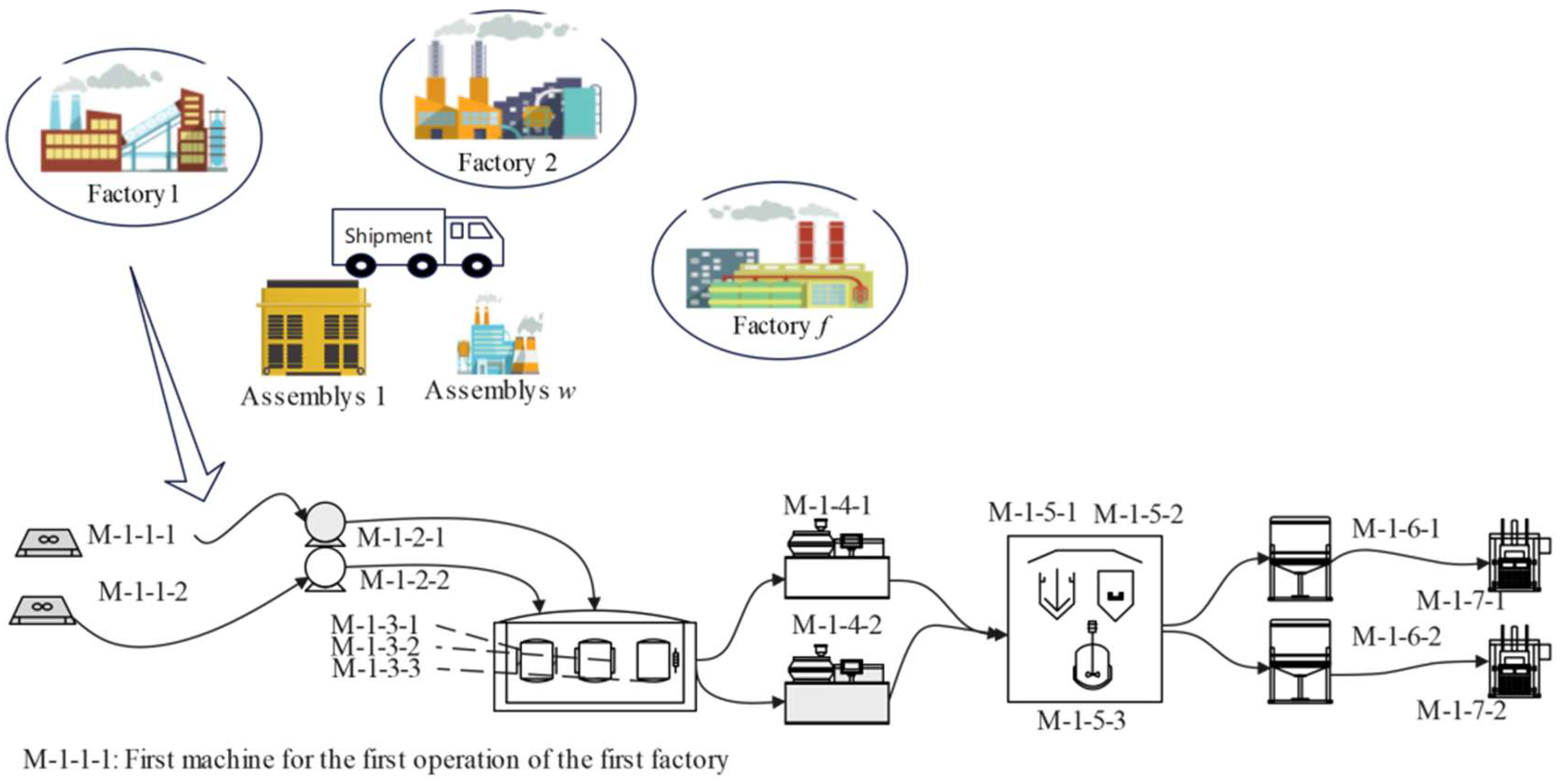
Figure 1. Process of DHFSTFA.
Symmetry 17 01306 g001
Figure 2. Comparison between with and without blocking scheduling for a solution.
Symmetry 17 01306 g002
Figure 3. Flow of QNSGA.
Symmetry 17 01306 g003
Figure 4. Partial representation of neighborhood structures.
Symmetry 17 01306 g004
Figure 5. Two crossover operators.
Symmetry 17 01306 g005
Figure 6. Experimental Methodology.
Symmetry 17 01306 g006
Figure 7. Mean plots accompanied by 95% Least Significant Difference (LSD) intervals for QNSGA parameters.
Symmetry 17 01306 g007
Figure 8. Mean plots with 95% LSD intervals for RPD values of eight variants and QNAGSA in three metrics.
Symmetry 17 01306 g008
Figure 9. Distribution of count rates for six search operators during large-scale iterations.
Symmetry 17 01306 g009
Figure 10. Mean plots with 95% LSD intervals for RPD values of state-of-the-art algorithms in three metrics.
Symmetry 17 01306 g010
Figure 11. Pareto front solutions of state-of-the-art algorithms in twelve cases.
Symmetry 17 01306 g011
Figure 12. Objectives comparison among metaheuristics and QNSGA during iteration.
Symmetry 17 01306 g012
Figure 13. Gantt chart comparison between heuristic solution and QNSGA solution. (a) Scheduling Gantt chart of the initial solution; (b) Scheduling Gantt chart of QNSGA.
Symmetry 17 01306 g013
Table 1. Possible States of the Population in the tth Iteration.
StateIndicatorStateIndicator
S 1 N f t = 0 , L t = 0 , T D t = 0 S 7 N f t = 1 , L t = 0 , T D t = 1
S 2 N f t = 0 , L t = 1 , T D t = 0 S 8 N f t = 1 , L t = 1 , T D t = 1
S 3 N f t = 0 , L t = 0 , T D t = 1 S 9 N f t = 2 , L t = 0 , T D t = 0
S 4 N f t = 0 , L t = 1 , T D t = 1 S 10 N f t = 2 , L t = 1 , T D t = 0
S 5 N f t = 1 , L t = 0 , T D t = 0 S 11 N f t = 2 , L t = 0 , T D t = 1
S 6 N f t = 1 , L t = 1 , T D t = 0 S 12 N f t = 2 , L t = 1 , T D t = 1
Table 2. Eight actions in the construction of QNSGA.
ActionIndicatorActionIndicator
A 1 C 1 + V N S 1 + A c c 1 A 5 C 2 + V N S 2 + A c c 1
A 2 C 2 + V N S 1 + A c c 1 A 6 C 2 + V N S 1 + A c c 2
A 3 C 1 + V N S 2 + A c c 1 A 7 C 1 + V N S 2 + A c c 2
A 4 C 1 + V N S 1 + A c c 2 A 8 C 2 + V N S 2 + A c c 2
Table 3. Parameters settings for both small- and large-scale problems.
ParameterSmallLarge
t{3, 5, 8}{10, 30, 50}
m{2, 3, 4}{6, 8, 10}
f{2, 3, 4}{5, 6, 8}
|Ph|{2, 4}{10, 15}
w⌈t/2⌉⌈t/2⌉
KilRandSelect {1,2,3}RandSelect {1,2,3,4,5}
pjkU [1,99]U [1,99]
qha [ 1 N h , 99 N h ] [ 1 N h , 99 N h ]
r g a j U [1,49]U [1,49]
dh ( j = 1 n p j y j h + a = 1 w q h a ) / f ( j = 1 n p j y j h + a = 1 w q h a ) / f )
Table 4. Taguchi experimental results of QNSGA.
No.N ϵ α γ RV
111110.09
212220.11
313330.09
414440.12
521230.12
622140.15
723410.09
824320.08
931340.06
1032430.06
1133120.06
1234210.03
1341420.01
1442310.01
1543240.08
1644130.01
I0.100.080.080.06
II0.110.080.090.07
III0.050.080.070.07
IV0.030.060.100.10
R0.080.020.030.05
Table 5. Computational results of RPD and CPU time (seconds) for the MILP solver and QNSGA on small-scale instances (best bolded).
InstanceMILP SolverQNSGA
CmaxTmaxTimeCmaxTmaxTime
MeanSTDMeanSTDMeanSTDMeanSTD
t30.0000.0000.0000.000345.210.0840.0130.0130.01427
50.1460.0230.0210.0291404.290.1500.0220.0450.02245
80.2430.1010.0320.0511887.670.1530.0250.0790.04172
m20.0150.0170.0160.0221162.250.0660.0130.0130.01732
30.1270.0250.0220.0321152.810.1000.0130.0490.02448
40.3000.0430.0300.0551680.750.2200.0210.0750.04064
f20.2400.0350.0310.0451679.100.1740.0220.0780.03532
30.1230.0190.0210.0251248.820.1190.0170.0430.01848
40.0790.0130.0170.0171067.890.0930.0130.0160.01364
|Ph|20.0960.0160.0130.0211297.780.0740.0150.0260.01648
40.1990.0270.0320.0441451.480.1830.0210.0650.03548
Average0.1300.0290.0210.0311307.10.1290.0180.0460.02548
Table 6. Average RPD values on three metrics comparing variants and QNSGA in large-scale instances (best results bolded).
a. Based on the Δ metric
Instance V 1 V 2 V 3 V 4 V 5 V 6 V 7 V 8 QNSGA
t100.1380.1640.2010.2170.2590.3090.3330.3670.1110
300.1590.1790.2250.2250.3070.3260.3510.4080.1245
500.1730.2090.2270.2400.3130.3500.3780.4410.1464
m60.1400.1640.1920.2090.2670.3130.3110.3690.1042
80.1580.1880.2220.2310.2850.3320.3480.3910.1269
100.1720.1980.2390.2420.3280.3400.4030.4560.1499
f50.1700.2150.2320.2520.3170.3550.4050.4390.1442
60.1550.1770.2160.2230.2980.3270.3520.3980.1253
80.1450.1590.2050.2060.2650.3040.3060.3790.1124
|Ph|100.1480.1700.2120.2130.2980.3170.3320.3890.1250
150.1660.1970.2230.2410.2890.3400.3760.4210.1296
Average 0.1570.1840.2180.2270.2930.3280.3540.4050.1273
b. Based on the GD metric
Instance V 1 V 2 V 3 V 4 V 5 V 6 V 7 V 8 QNSGA
t100.0590.0710.0850.0860.1150.1330.1410.1620.042
300.0620.0780.0870.0980.1290.1400.1450.1690.044
500.0670.0830.0960.1020.1340.1560.1570.1890.049
m60.0590.0700.0820.0850.1170.1290.1420.1510.040
80.0600.0730.0870.0940.1250.1310.1480.1650.044
100.0680.0890.0990.1070.1360.1680.1540.2040.050
f50.0680.0820.1010.1010.1370.1510.1670.1830.047
60.0640.0760.0870.0950.1240.1440.1490.1720.045
80.0550.0750.0800.0890.1180.1330.1270.1630.041
|Ph|100.0600.0730.0840.0880.1210.1290.1400.1710.044
150.0650.0820.0950.1020.1310.1570.1550.1750.046
Average 0.0620.0780.0890.0950.1260.1430.1480.1730.045
c. Based on the IGD metric
Instance V 1 V 2 V 3 V 4 V 5 V 6 V 7 V 8 QNSGA
t100.0060.0070.0090.0080.0120.0140.0140.0170.005
300.0070.0080.0090.0110.0140.0150.0160.0180.005
500.0080.0090.0100.0120.0140.0140.0180.0210.005
m60.0060.0080.0090.0080.0110.0130.0150.0160.005
80.0070.0080.0090.0090.0130.0150.0160.0190.005
100.0080.0090.0100.0130.0160.0160.0180.0210.005
f50.0080.0080.0100.0110.0140.0150.0180.0200.006
60.0070.0080.0100.0100.0140.0150.0160.0200.005
80.0070.0080.0090.0090.0120.0130.0150.0170.004
|Ph|100.0070.0070.0090.0100.0130.0130.0150.0170.005
150.0070.0090.0100.0100.0140.0160.0180.0210.005
Average 0.0070.0080.0090.0100.0140.0140.0160.0190.005
Table 7. Friedman test results of comparison between variants and QNSGA in large-scale instances.
Metric V 1 V 2 V 3 V 4 V 5 V 6 V 7 V 8 QNSGA
Δ3.4213.7684.3084.2075.6076.4457.1058.3392.902
p-value0.000
GD2.9143.3204.3424.3416.1436.5126.6927.9662.068
p-value0.000
IGD2.8933.1734.3114.5116.1006.5977.3748.5882.375
p-value0.000
Table 8. Average RPD values on three metrics comparisons between state-of-the-art algorithms in large-scale instances (best results bolded).
a. Based on the Δ metric
Instance MOPSOQSFLRLABCCWWORLCMAFSNSGAQNSGA
t105.68 × 10−35.14 × 10−36.18 × 10−36.40 × 10−35.54 × 10−33.02 × 10−33.15 × 10−3
308.14 × 10−37.06 × 10−37.87 × 10−37.80 × 10−37.87 × 10−36.31 × 10−35.22 × 10⁻³
501.13 × 10−21.01 × 10−21.08 × 10−29.04 × 10−39.42 × 10−39.25 × 10−39.19 × 10⁻³
m65.64 × 10−35.29 × 10−36.06 × 10−36.38 × 10−35.67 × 10−33.12 × 10−33.17 × 10−3
87.85 × 10−37.15 × 10−37.90 × 10−38.09 × 10−38.10 × 10−36.95 × 10−36.22 × 10⁻³
101.16 × 10−29.86 × 10−31.09 × 10−28.77 × 10−39.07 × 10−38.52 × 10−38.18 × 10⁻³
f51.15 × 10−21.01 × 10−21.04 × 10−29.34 × 10−39.52 × 10−39.06 × 10−38.67 × 10−3
67.86 × 10−36.99 × 10−38.16 × 10−37.51 × 10−37.65 × 10−36.55 × 10−35.95 × 10⁻³
85.79 × 10−35.18 × 10−36.30 × 10−36.39 × 10−35.67 × 10−32.97 × 10−32.94 × 10⁻³
|Ph|106.91 × 10−36.10 × 10−37.02 × 10−37.10 × 10−36.71 × 10−34.13 × 10−34.09 × 10⁻³
159.85 × 10−38.77 × 10−39.55 × 10−38.40 × 10−38.52 × 10−38.25 × 10−37.62 × 10⁻³
Average 8.38 × 10−37.44 × 10−38.28 × 10−37.75 × 10−37.61 × 10−36.19 × 10−35.86 × 10⁻³
b. Based on the GD metric
Instance MOPSOQSFLRLABCCWWORLCMAFSNSGAQNSGA
t104.67 × 10−53.75 × 10−54.70 × 10−54.03 × 10−54.10 × 10−53.25 × 10−52.73 × 10−5
306.12 × 10−55.70 × 10−56.37 × 10−55.58 × 10−55.94 × 10−55.94 × 10−54.79 × 10⁻⁵
507.22 × 10−58.38 × 10−58.42 × 10−58.04 × 10−58.92 × 10−57.54 × 10−57.25 × 10⁻⁵
m64.52 × 10−53.89 × 10−54.67 × 10−54.23 × 10−54.24 × 10−53.36 × 10−52.77 × 10−5
86.24 × 10−55.90 × 10−56.45 × 10−55.63 × 10−55.71 × 10−56.02 × 10−54.89 × 10⁻⁵
107.24 × 10−58.05 × 10−58.37 × 10−57.80 × 10−59.01 × 10−57.35 × 10−57.11 × 10⁻⁵
f57.24 × 10−57.05 × 10−58.37 × 10−57.80 × 10−59.01 × 10−57.35 × 10−57.61 × 10−5
66.03 × 10−55.99 × 10−56.35 × 10−55.76 × 10−55.85 × 10−56.29 × 10−55.02 × 10⁻⁵
84.73 × 10−54.79 × 10−54.77 × 10−54.09 × 10−54.10 × 10−53.09 × 10−52.14 × 10⁻⁵
|Ph|105.38 × 10−54.89 × 10−55.56 × 10−54.93 × 10−54.97 × 10−54.69 × 10−53.83 × 10⁻⁵
156.62 × 10−57.00 × 10−57.43 × 10−56.84 × 10−57.67 × 10−56.47 × 10−56.02 × 10⁻⁵
Average 6.00 × 10−55.95 × 10−56.50 × 10−55.88 × 10−56.32 × 10−55.58 × 10−54.93 × 10⁻⁵
c. Based on the IGD metric
Instance MOPSOQSFLRLABCCWWORLCMAFSNSGAQNSGA
t101.24 × 10−31.13 × 10−31.16 × 10−31.85 × 10−31.87 × 10−31.02 × 10−31.11 × 10−3
302.33 × 10−32.00 × 10−32.33 × 10−32.20 × 10−33.21 × 10−31.92 × 10−31.50 × 10⁻³
504.07 × 10−33.53 × 10−33.76 × 10−33.37 × 10−34.27 × 10−32.95 × 10−32.42 × 10⁻³
m61.45 × 10−31.33 × 10−31.32 × 10−31.92 × 10−31.85 × 10−31.06 × 10−31.25 × 10−3
82.41 × 10−32.04 × 10−32.34 × 10−32.31 × 10−33.18 × 10−31.94 × 10−31.56 × 10⁻³
103.78 × 10−33.29 × 10−33.59 × 10−33.19 × 10−34.33 × 10−32.89 × 10−32.22 × 10⁻³
f53.18 × 10−33.12 × 10−33.14 × 10−33.26 × 10−34.33 × 10−32.98 × 10−32.63 × 10−3
62.46 × 10−32.07 × 10−32.41 × 10−32.20 × 10−33.14 × 10−31.74 × 10−31.57 × 10⁻³
82.00 × 10−31.47 × 10−31.70 × 10−31.96 × 10−31.89 × 10−31.17 × 10−38.34 × 10⁻⁴
|Ph|101.83 × 10−31.58 × 10−31.73 × 10−32.11 × 10−32.51 × 10−31.50 × 10−31.40 × 10⁻³
153.26 × 10−32.86 × 10−33.10 × 10−32.83 × 10−33.72 × 10−32.43 × 10−31.95 × 10⁻³
Average 2.55 × 10−32.22 × 10−32.42 × 10−32.47 × 10−33.12 × 10−31.96 × 10−31.68 × 10⁻³
Table 9. Friedman test results of comparison between state-of-the-art algorithms in large-scale instances.
Metric.MOPSOQSFLRLABCCWWORLCMAFSNSGAQNSGA
Δ6.5553.0437.5044.2124.1392.5672.184
p-value0.000
GD6.0773.0417.4163.9994.2962.7902.347
p-value0.000
IGD6.3503.7907.1264.2235.3233.3532.863
p-value0.000
Disclaimer/Publisher’s Note: The statements, opinions and data contained in all publications are solely those of the individual author(s) and contributor(s) and not of MDPI and/or the editor(s). MDPI and/or the editor(s) disclaim responsibility for any injury to people or property resulting from any ideas, methods, instructions or products referred to in the content.