Abstract
Accurate estimation of heterogeneous treatment effects (HTEs) serves as a cornerstone of personalized decision-making, especially in observational studies where treatment assignment is not randomized. However, the presence of confounding and complex covariate structures poses significant challenges to reliable inference. In this study, we develop an innovative model averaging framework, which leverages proximity-based matching to enhance the accuracy of HTE estimation. The method constructs pseudo-outcomes via proximity score matching and subsequently applies an optimal model averaging procedure to these matched samples. We demonstrate that the proposed estimator achieves asymptotic optimality when the standard regularity conditions are met. Simulation studies, adapted from benchmark settings for evaluating HTE model averaging, confirm its superior finite-sample performance. Compared to standard HTE estimation approaches, the proposed method achieves consistently lower estimation errors and reduced variability. The method is further validated on a clinical dataset from the CPCRA trial, demonstrating its practical value for individualized causal inference.
1. Introduction
Identifying how binary interventions influence outcomes represents a central challenge in both statistics and econometrics, with extensive applications across fields such as economics, healthcare, marketing, and policy analysis. Classical examples include the evaluation of job training programs, college education, and medical interventions [1,2,3]. In empirical research, it is often essential to move beyond estimating the average treatment effect (ATE) and explore how treatment responses vary among individuals—referred to as heterogeneous treatment effects (HTEs). Understanding HTE is critical for personalized interventions, policy targeting, and efficient resource allocation [4,5].
Traditional approaches to causal inference, such as linear regression or difference-in-means estimators, typically assume constant treatment effects and rely on strict parametric conditions. These limitations have motivated the development of flexible, data-driven methods for HTE estimation. Representative examples include Bayesian Additive Regression Trees (BART) [6,7], causal trees [8], and causal forests [5]. While these methods offer greater flexibility and improved detection of effect heterogeneity, they also introduce new challenges, such as model uncertainty, sensitivity to model specification, and potential overfitting in finite samples.
Averaging across multiple candidate models has become a well-established approach to mitigate the risks of model uncertainty, as opposed to depending on a single model choice. Early studies in this area emphasized Bayesian Model Averaging (BMA), which utilizes Bayes’ theorem to compute posterior weights for candidate models and enables statistically consistent inference when appropriate priors are specified [9,10,11]. In addition to Bayesian methods, numerous model averaging techniques have been proposed from a frequentist perspective. A number of these approaches incorporate smoothed likelihood-based criteria, including SAIC, SBIC, and SFIC [12,13,14].
To further improve predictive performance and robustness, adaptive model averaging methods have also been proposed. Notable examples include Adaptive Regression by Mixing (ARM) and its L1-penalized variant (L1-ARM), which estimate model weights directly from data with theoretical guarantees [15,16,17]. Other methods aim to minimize prediction risk, including Mallows Model Averaging (MMA) [18,19], Jackknife Model Averaging (JMA) [20], KL-divergence–based methods [21,22], and Parsimonious Model Averaging (PMA) [23].
Although much of the existing research emphasizes the estimation of overall treatment effects, recent developments have adapted model averaging techniques to the study of heterogeneous effects. In observational settings, Seng and Li [24] proposed a model averaging method that incorporates instruments into a two-stage estimation routine for treatment effect inference. A method for model averaging that seeks to minimize the approximate mean squared error for semiparametric estimators was developed by [25]. More directly related to HTE, Rolling et al. [26] constructed weights via nearest neighbor matching and derived finite-sample risk upper bounds, whereas Zhao et al. [27] also utilized nearest neighbor matching but focused on achieving asymptotic optimality of the CATE estimator. These developments highlight the growing interest in integrating model averaging with HTE estimation. In essence, model averaging provides a principled way to integrate the uncertainty across multiple HTE estimators, thereby yielding more robust and accurate treatment effect estimates in observational studies.
An essential stream of causal inference research involves matching techniques, designed to lessen confounding through the alignment of treated and untreated observations exhibiting analogous covariate patterns. Traditional approaches include exact matching, Mahalanobis distance matching [28,29], and the widely used propensity score matching [30,31]. These methods construct matched samples that approximate randomized experiments by balancing covariates between groups. Subsequent developments such as prognostic score matching [32] and full matching [33,34] further improve finite-sample performance and covariate balance.
Recent research has shifted toward data-adaptive and machine learning–enhanced matching strategies. For example, Gao et al. [35] proposed proximity score matching based on random forests to measure unit similarity. Their combo (Proximity score distance with FACT matching)method solves an optimal assignment problem using proximity distances, yielding better covariate balance and improved estimation efficiency compared to classical matching algorithms. These innovations pave the way for adaptive matching methods in the context of HTE estimation.
Despite these advances, the integration of matching strategies and model averaging techniques remains theoretically underdeveloped. In particular, few studies have rigorously examined the optimality properties of model averaging estimators based on matched samples. Bridging this gap is crucial for constructing robust procedures that leverage both model-based and design-based inference principles.
In this study, a new methodological framework is introduced to estimate HTEs through the integration of proximity matching and model averaging. We adopt the proximity matching approach of [35] to construct high-quality pseudo-observations and integrate it with a penalized model averaging procedure tailored to the matched sample. We construct an optimal weight selection rule aimed at reducing an asymptotically unbiased estimate of the expected prediction error, and prove that the resulting estimator achieves asymptotic optimality under standard regularity conditions. Our contributions extend classical model averaging theory to matched-design settings and establish a principled foundation for combining these two powerful paradigms in HTE estimation. Compared to the partition matching strategy used in [27], our method employs proximity score matching, which enables more adaptive unit pairing and demonstrates superior empirical performance in simulation studies.
To evaluate the effectiveness of our approach, we carry out comprehensive simulation experiments adapted from [35], specifically designed to evaluate model averaging estimators. The proposed framework demonstrates consistent advantages over standard alternatives, including selection-based strategies and model averaging methods without proximity integration, in terms of estimation precision and predictive reliability. These findings underscore the practical utility and theoretical soundness of our approach in modern causal inference settings. While prior literature has explored model averaging and matching separately for treatment effect estimation, the integration of these two approaches remains underdeveloped. Our study addresses this gap by proposing a unified framework that leverages proximity-based matching to construct pseudo-observations and applies model averaging to mitigate estimator instability. This joint approach improves robustness to model misspecification and enhances accuracy in heterogeneous treatment effect estimation, especially in observational studies with complex covariate structures.
The contributions of this work are summarized below.
- We introduce a novel HTE estimation framework that combines proximity matching with model averaging, addressing both model uncertainty and matching-induced bias.
- The resulting estimator, constructed under the combo matching framework, is shown to achieve asymptotic optimality through a derived optimal weighting criterion.
- We validate the proposed method through simulation studies, demonstrating superior performance over existing approaches.
The subsequent sections are organized as outlined below. We begin in Section 2 by outlining the proposed approach, which integrates proximity matching with model averaging. Section 3 develops the theoretical results and establishes asymptotic optimality. Section 4 presents the simulation results, while Section 5 illustrates the method with a real-world dataset. Section 6 concludes with a discussion of future directions. Proofs of the theoretical results appear in Appendix A. Appendix B includes the PM-OPT pseudocode along with summaries of key notations and abbreviations for ease of reference.
2. Methodology
This section outlines our approach to estimating HTEs through the combination of proximity matching and model averaging. We first present the structural assumptions and model setup, including the potential outcomes framework and the definition of CATE. Next, we describe the construction of pseudo-observations based on proximity matching, followed by the formulation of multiple candidate models. Finally, we introduce the model averaging procedure and a penalized criterion for weight selection that ensures asymptotic optimality. Together, these components form a unified and robust estimation strategy for HTEs.
2.1. Model Framework and Assumptions
We begin by introducing the general framework and notations. Denote by the observed covariates, treatment, and outcome for unit i, with . These units are assumed to be drawn i.i.d. from the population. For each unit, we observe a covariate vector , a binary treatment indicator (where indicates treatment assignment, with 1 representing treated units and 0 indicating controls), and an outcome variable .
Under the potential outcomes framework [30], each unit i is associated with a pair of potential responses: if treated, and if untreated. The observed response is
which implicitly relies on the Consistency assumption.
Assumption 1
(Consistency). For each unit i, the observed outcome equals the potential outcome under the received treatment: .
This assumption presumes no interference between units and a well-defined treatment assignment, commonly referred to as the Stable Unit Treatment Value Assumption (SUTVA).
The primary estimand of interest is the CATE
which quantifies how the causal effect varies with covariates. We estimate and separately on the treated and control samples, respectively, using linear regression models without including the treatment indicator or interaction terms in the design matrices. The HTE function is defined as the difference between the two fitted functions.
To nonparametrically identify from observational data, we impose the following standard assumptions.
Assumption 2
(Unconfoundedness).
Assumption 3
(Overlap). There exists a constant such that for all x in the support of X,
Assumption 2 rules out unmeasured confounding, while Assumption 3 ensures that both treatment and control groups are sufficiently represented at each covariate value. Together, Assumptions 1–3 guarantee the identifiability of .
In this paper, we further assume a structural model for the potential outcomes of the form
where and are unknown regression functions, and is a mean-zero error term with finite variance.
Assumption 4
(Error Structure).
- (i)
- for ;
- (ii)
- ;
- (iii)
- The error terms and are independent for .
Assumption 4 specifies a standard error structure often adopted in causal inference literature. Part (i) assumes that the error terms have zero conditional mean given the covariates, ensuring that the systematic component captures all predictable variation in potential outcomes. Part (ii) imposes that the error variances are finite and may differ between treatment groups, which allows for heteroskedasticity but ensures well-behaved inference. Part (iii) assumes that the error terms are independent across units, meaning that and are independent for . This cross-unit independence is typical in cross-sectional settings and supports valid asymptotic analysis. We do not require and to be independent, as only one potential outcome is observed per unit. This pruning strategy ensures that the resulting matched graph consists of small connected components, each containing at most one treated (or control) unit. As a result, the matched residuals are unlikely to exhibit cross-unit dependence, supporting the plausibility of the independence assumption in Assumption 4 (iii); see [35] for related discussion.
Given this structure, the observed outcome model becomes
where .
Under this formulation, the CATE is equivalently expressed as
This setup forms the foundation for the model averaging estimator developed in the following sections. Our goal is to estimate by combining multiple candidate models fitted on proximity-matched samples, and to establish theoretical guarantees for its asymptotic performance.
2.2. Candidate Models and Model Averaging Formulation
To estimate the CATE function , we employ a model averaging strategy based on linear candidate models. Each candidate model approximates the potential outcome functions for using a different subset of covariates. This construction explicitly accounts for model uncertainty in variable selection.
Let there be K candidate models indexed by . Denote by the index set of covariates used in model , and let denote the subvector of corresponding to the covariates in , where . Then, model approximates the outcome model as
where are model-specific coefficients for treatment group , and are mean-zero errors. We emphasize that the true functions and are not assumed to be linear; instead, we approximate them via linear least squares within each candidate model, following standard practice in model averaging under potential misspecification.
For model , we estimate and using least squares on the treated and control samples, respectively. Let and denote the design matrices of treated and control units under model , and , the corresponding outcomes. Then the estimators are given by
At covariate value x, the CATE estimated by model is
Let be model weights satisfying
We define the model averaging estimator of as a convex combination of the K candidate estimators
Since , the model averaging estimator represents a convex combination of the candidate estimators , ensuring the final estimator lies within their convex hull. This estimator allows for improved robustness to model misspecification by integrating information across diverse model structures. The subsequent sections introduce our proximity-matching-based strategy for constructing pseudo-observations and describe how we select the weight vector by minimizing an empirical approximation of the conditional prediction risk.
3. Weight Choice and Asymptotic Optimality
In this section, we present the methodology for determining optimal model averaging weights in the context of proximity-matched pseudo-observations. We begin by describing the construction of matched pairs via the combo matching approach. Building on this, we formulate a risk-based criterion for weight selection tailored to treatment effect estimation. We then rigorously analyze the asymptotic behavior of the resulting estimator and establish its optimality under a set of regularity conditions.
The proposed PM-OPT framework extends conventional model averaging approaches by integrating proximity-based matching to construct pseudo-outcomes, enabling more accurate estimation of heterogeneous treatment effects. Compared to existing methods such as OPT or TEEM, PM-OPT leverages local balance through matching and aggregates predictions across multiple models using a risk-based weighting scheme. This integration not only improves robustness against model misspecification and sampling variability, but also offers a practical pathway for applying model averaging in causal inference settings where high-quality matching is difficult to achieve.
3.1. Proximity Matching and Pseudo-Observations
We adopt the combo matching strategy introduced in Gao et al. [35], which combines full matching constraints with average distance minimization. Compared to propensity score matching and nearest-neighbor matching, combo matching simultaneously achieves global covariate balance and local similarity through a constrained optimization framework based on proximity score distances. The proximity score distance is a model-based measure of similarity between units, computed from an auxiliary predictive model such as random forests or gradient boosting trees. It reflects how often two units fall into the same terminal nodes across trees, capturing nonlinear relationships and interactions among covariates. This allows the matching procedure to account for complex patterns in the covariate space beyond what traditional distances can capture. To enforce balance and reduce estimation variance, the algorithm constructs a matching graph with a path length constraint of at most three. This structure prevents the formation of large connected components and ensures that each unit appears in at most one matched pair. A pruning procedure is applied to iteratively remove redundant or suboptimal edges from the matching graph, ensuring that each unit appears in at most one matched pair while preserving high-quality matches. This design allows matched units to remain in the same validation fold during sample splitting, thereby avoiding the breakdown of pseudo-outcomes and ensuring low-variance estimates. In the context of PM-OPT, combo matching provides stable and informative matched pseudo-observations that are critical for accurately estimating HTEs.
Let L denote the total number of matched treatment-control pairs constructed using the combo algorithm [35]. For each matched pair indexed by , let denote the indices of the treated and control units, respectively. The observed covariates and outcomes are denoted as and , with and .
Under the potential outcomes framework, a pseudo-treatment effect is defined for every matched pair of units
where the decomposition includes
- representing the bias due to imperfect covariate matching;
- representing the composite noise from both units.
To ensure the validity of the pseudo-outcomes, it is important to control the bias term . Under the assumption that the regression functions satisfy a smooth continuity condition, and the covariate space is compact, the combo algorithm ensures high-quality matches in the covariate space.
Lemma 1.
Suppose the function is smooth over a compact domain in the sense that its local variation over matched covariate pairs is bounded by a constant multiple of for some . Then, under the proximity matching procedure, the matching bias is uniformly bounded as
where p is the covariate dimension and the result holds for sufficiently well-matched pairs.
Proof.
Under the assumption that is smooth continuous with exponent , we have
According to Gao et al. [35], the combo matching algorithm minimizes the total matching cost based on proximity scores from a random forest, which effectively controls the pairwise distance between matched treated and control units. In high-dimensional settings, it is well established (e.g., [3]) that proximity-based matching yields a rate . Combining this with the smooth condition yields
uniformly over all matched pairs . □
This result implies that, under smoothness conditions and sufficiently accurate matching, the deviation of the pseudo-outcome from the true conditional average treatment effect decays at a polynomial rate as the sample size n increases.
Remark 1.
Although prior empirical evidence ([35]) indicates that combo matching yields low estimation bias, our result formalizes this observation by linking the bias to smoothness conditions on the outcome function and deriving an explicit convergence rate.
3.2. Weight Choice Criterion
Given the matched treatment-control pairs constructed using the combo matching algorithm, define the pseudo-outcome for each pair as
and let be the vector of all pseudo-treatment effects.
For each candidate model , define the vector of predicted treatment effects evaluated at the treated units as
Let and denote the full design matrices of the treated and control units under model , respectively. Let and be the corresponding submatrices for the matched pairs, where the rows correspond to the units and , respectively.
We define the individual projection matrices as
The model-averaged projection matrices are defined as
where denotes the model averaging weights.
To align dimensions with the full length L, we define the zero-padded projection matrices as
and their corresponding model-averaged forms are
We define the penalized criterion as
where and are the noise variances for the treated and control groups, respectively.
The optimal weight is obtained by
Let denote the corresponding vector of true CATEs, and define the squared error loss and conditional risk of as
where denotes the observed covariates used in the projection matrices. We determine the weight vector by minimizing an empirical approximation of the risk function .
Theorem 1
(Asymptotic Unbiasedness). Provided that . Then, the penalized criterion satisfies
uniformly over .
Proof.
See Appendix A.1. □
Remark 2.
This result shows that the weight selection criterion serves as an asymptotically unbiased estimator of the conditional risk up to a constant. The combo-matching framework ensures that the approximation error is sufficiently small, and the projection-based penalty terms control the model complexity.
3.3. Asymptotic Optimality
In this section, we show that our proposed model averaging estimator under combo matching enjoys an asymptotic optimality property. Unless otherwise stated, all limiting processes discussed in this and subsequent sections are with respect to .
Now, write , and let be the model-averaged predictions based on the treatment and control arms respectively, where and .
We define the squared error and the conditional risk as
Now, write . The subsequent theoretical analysis will be based on these conditional risk functions.
Condition 1
(Moment condition). For all matched pairs , and some fixed integer ,
Condition 1 imposes a uniform bound on the conditional moments of the pseudo-error terms across all matched pairs. This type of moment condition is standard in the matching literature and is similar to condition (7) in [19] and condition (17) in [27]. This condition is readily satisfied when the error terms follow Gaussian or sub-Gaussian distributions, which are common in practice.
Condition 2
(Risk concentration condition). Let denote the unit vector with 1 at the kth position. And,
Condition 2 resembles Condition (8) in [19] and is also related to the bias-variance trade-off condition discussed in [18,27]. This assumes that the true model is not exactly contained in the candidate model set, which is a standard and realistic assumption in the model averaging literature. In practice, all candidate models are usually simplified approximations of the data-generating process, especially when the model space is of moderate size and does not exhaust all possible higher-order interactions. This condition ensures that the approximation bias does not vanish entirely, aligning with the setup commonly adopted in nonparametric regression frameworks (see [18]).
Condition 3
(Minimum eigenvalue condition). For each , there exist constants such that
where denotes the smallest eigenvalue of a symmetric matrix.
Condition 3 is a minimum eigenvalue condition, ensuring sufficient identifiability of the covariate design matrix within each candidate model. This requirement aligns with condition C.4 of [22] and condition 1 of [36], and is necessary for ensuring the stability of least squares estimators and the convergence of projection matrices. This condition is generally easy to satisfy in practice, as it only requires that the covariates are not perfectly collinear and have reasonable variation, which is common in empirical data sets.
Condition 4
(Growth condition).
Condition 4 restricts the relative growth rates of the matched sample size L, the number of covariates p, and the bias decay rate parameter . Such a condition is commonly required in matched sampling frameworks to ensure that the approximation bias induced by matching does not dominate the overall estimation error. In our setting, it reflects a balance between the smoothness of the regression functions and the size of the matched sample. For instance, when the bias decay rate satisfies for some , Condition 4 can be satisfied by choosing with sufficiently small , especially when the regression functions are smooth (i.e., large ).
Theorem 2
(Asymptotic Optimality). Suppose Assumptions 1–4 and Conditons 1–4 hold, and the number of matched pairs satisfies as . Then the model averaging estimator satisfies
i.e., the model averaging estimator achieves asymptotic optimality among all convex combinations of the K candidate models.
Proof.
See Appendix A.2. □
Remark 3.
When and are replaced by consistent estimators and , Theorem 2 remains valid under mild regularity conditions. The literature provides similar insights, for instance in Hansen [18] and Zhao et al. [27].
4. Numerical Experiments
This section evaluates the effectiveness of Proximity Matching OPT estimator (“Proximity Matching OPT” (PM-OPT) denotes the proximity–matching criterion with the OPT weight solution). against several competing model averaging methods under a comprehensive set of simulation scenarios. All simulations are implemented in R, and each setting is replicated 1000 times to ensure stable Monte Carlo error. The evaluation focuses on each method’s ability to estimate HTEs across multiple experimental designs, differing in treatment assignment mechanisms, functional forms of effect heterogeneity, signal-to-noise ratios (SNR), and sample sizes. The code used for the numerical results section is available on our GitHub repository at https://github.com/zhzhao07 (accessed on 4 August 2025).
4.1. Simulation Design
We conduct a series of simulation experiments to systematically compare the performance of various model selection and model averaging methods for estimating HTEs. Specifically, we evaluate classical criteria such as the Akaike Information Criterion (AIC) and Bayesian Information Criterion (BIC); their smoothed model averaging extensions, SAIC and SBIC [12]; treatment-effect-oriented criteria including the Treatment Effect Cross-Validation (TECV) criterion [37] and the Treatment Effect Estimation by Mixing (TEEM) method [26]; the asymptotically optimal averaging method OPT [27]; and the proposed Proximity-Matching-based Optimal Averaging method, PM–OPT. The simulation designs are crafted to reflect realistic challenges in observational data, including model misspecification, covariate imbalance, and treatment effect heterogeneity. In our study, the parameters for the Proximity matching and Prognostic score distance were determined by optimizing the out-of-bag (OOB) mean-squared error of the random forest. These settings follow the methodology outlined by [35]. Specifically, we used the same settings for the number of trees and the number of variables randomly sampled at each split in the random forest to compute the proximity scores. This ensures consistency with previous work and reliable comparisons. For the other model estimation processes, no additional tuning parameters were adjusted, as we focused on maintaining consistency and comparability across the methods.
The AIC and BIC are well-established model selection criteria that identify a single best model by trading off goodness-of-fit with model complexity. For the kth candidate model, we define the residual variance as
and compute the scores
denotes the model complexity (i.e., number of parameters) in .
To mitigate model selection uncertainty, ref. [12] proposed SAIC and SBIC estimators, which form model averages rather than choosing a single model. The weight assigned to model k under SAIC is given by
with an analogous formulation for SBIC based on BIC scores.
Recognizing the limitations of prediction-based criteria in causal inference settings, ref. [37] introduced the TECV criterion, which selects models based on their accuracy in estimating treatment effects. Building on this, ref. [26] developed the TEEM method, a computationally intensive approach that adaptively averages models to minimize conditional treatment effect estimation error.
We also include the OPT method proposed by [27], which determines averaging weights by minimizing an unbiased estimator of the mean squared error of the CATE estimator. This method enjoys strong asymptotic optimality guarantees under fixed-parameter asymptotics.
Finally, we introduce and evaluate our PM–OPT estimator, which extends the OPT approach by incorporating proximity-score-based matching [35] to construct pseudo-outcomes for both treatment and control groups. This matching step reduces bias from covariate imbalance, and the subsequent model averaging enhances robustness and finite-sample efficiency. Together, this two-stage strategy is designed to combine the strengths of flexible matching and asymptotically optimal model averaging for HTE estimation.
To form the pool of candidate models for averaging, we consider every possible combination of covariates along with their interaction terms with the treatment indicator. Given a dataset consisting of an outcome variable Y, a binary treatment indicator T, and a set of p covariates , we rename the covariates as for consistency. The model space is formed by taking the power set of these covariates, which yields subsets. For each subset , we construct a linear regression model that includes the treatment main effect T, the main effects of the covariates in , and the interaction terms between T and each covariate in . Accordingly, each model has the form
where denotes a error term. All candidate models are estimated via ordinary least squares. This full enumeration strategy ensures that the model averaging procedure operates over a rich and structured set of specifications, ranging from simple models with no covariates to complex ones that incorporate both covariate main effects and treatment–covariate interactions. The resulting model space captures a broad spectrum of potential treatment effect heterogeneity structures and facilitates a robust assessment of model averaging performance.
For each replication, we generate five covariates independently from a uniform distribution on the interval . Two treatment assignment mechanisms are considered. In the first case, treatment is assigned completely at random, so that the propensity score is fixed at . In the second case, the treatment assignment depends on the first covariate, with the propensity score modeled as .
To represent different forms of heterogeneity in treatment effects, we consider two types of true CATE. The linear CATE is specified as , while the nonlinear CATE takes the form .
We define the potential outcomes by , with the treatment outcome given by , where is an independent noise term and the baseline outcome function is given by .
To control the level of treatment effect signal relative to outcome noise, we follow [27] and define the SNR as the design-level quantity We vary over the grid to represent different levels of treatment signal strength. In each case, the function is scaled appropriately to ensure the empirical matches the desired target value.
Finally, we examine the performance of each method under three sample size regimes: (small), (medium), and (moderately large).
Each simulation scenario is repeated for replications. Estimator accuracy is evaluated based on their associated risk, quantified by the average squared error (ASE)
To enable fair comparison, we scale the risk by the corresponding value from the optimal least squares estimator (assumed to be infeasible) within each replication and design.
Table 1 compiles the four designs. Design A adopts the linear with random assignment; Design B keeps the linear effect but introduces covariate–dependent assignment; Design C employs the nonlinear under random assignment; Design D combines with the logistic propensity score.

Table 1.
Simulation settings.
Remark 4.
Although we adopt full enumeration of candidate models in the current low-dimensional setting, we acknowledge that this strategy does not scale well when the number of covariates increases. Several practical extensions are available to address this limitation. For moderately high-dimensional settings, nested models based on variable importance rankings or greedy model selection algorithms such as forward or backward selection can be used to generate a manageable model space. In higher-dimensional applications, it is common to apply Lasso-based variable preselection to screen covariates prior to constructing model subsets. In addition, within the context of HTE estimation, the model space can be further simplified by restricting interaction terms. For example, one may consider only main effects and exclude higher-order interactions, which reduces computational burden while maintaining interpretability.
4.2. Results
Following the simulation design and proximity matching setup in [35], we adopt the same covariate structure and distance metrics. Since [35] provides a comprehensive evaluation of the matching quality using standardized mean differences and other diagnostics, we do not replicate those assessments here to avoid redundancy.
Building upon the simulation framework described above, we now turn to the empirical evaluation of various model averaging strategies. The results, summarized in Figure 1, Figure 2, Figure 3 and Figure 4, highlight how each method adapts to changes in the data environment, revealing both the advantages and limitations of classical, smoothed, and targeted model averaging approaches. In what follows, we describe the main findings from each design in turn.
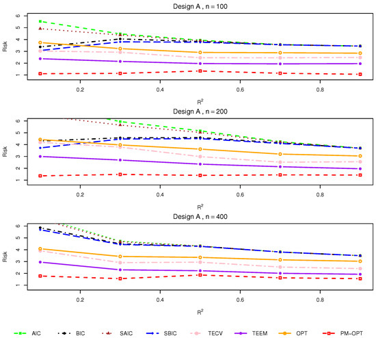
Figure 1.
Relative risks (lower is better) for Design A with .
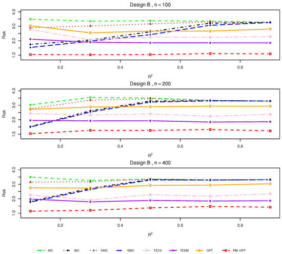
Figure 2.
Relative risks (lower is better) for Design B with .
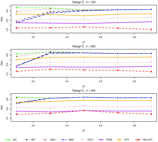
Figure 3.
Relative risks (lower is better) for Design C with .
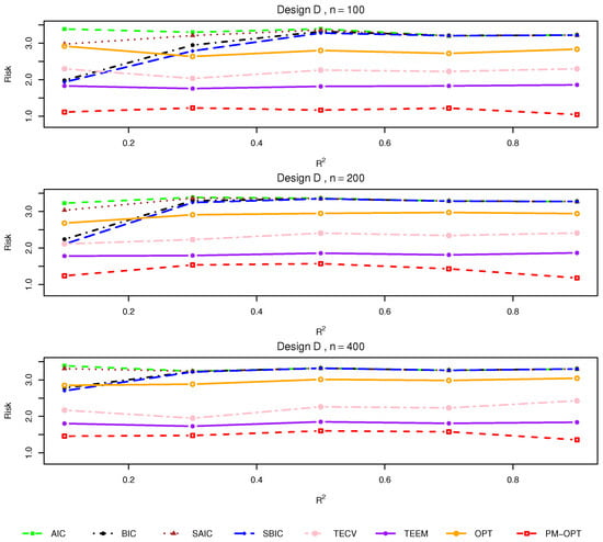
Figure 4.
Relative risks (lower is better) for Design D with .
Design A. This scenario features a linear treatment effect under randomized assignment. As shown in Figure 1, all methods perform similarly when the SNR is high and the sample size is moderate to large. However, under small sample sizes () or lower , traditional criteria such as AIC and BIC exhibit increased risk relative to more tailored approaches. Smoothed variants (SAIC and SBIC) consistently outperform their unsmoothed counterparts, particularly in low signal settings. The TECV and TEEM estimators demonstrate competitive performance throughout, while the proposed OPT and PM-OPT estimators achieve the lowest risks across nearly all configurations. The benefits of PM-OPT are especially apparent in smaller samples, where matching helps stabilize estimation.
Design B. Introducing covariate-dependent treatment assignment while maintaining linear treatment effects, Design B presents a more realistic observational setting. As illustrated in Figure 2, performance trends mirror those in Design A, but the relative advantage of targeted methods becomes more pronounced. The gap between OPT/PM-OPT and classical methods widens under moderate values, suggesting that accounting for assignment bias via flexible modeling and matching can lead to more accurate estimates. Notably, BIC deteriorates more sharply in small samples, reflecting its tendency toward overly parsimonious models in complex settings.
Design C. This setting imposes a nonlinear treatment effect structure under randomized assignment. The results in Figure 3 show that the performances of classical model averaging approaches (AIC, BIC, SAIC, SBIC) suffers under model misspecification. In contrast, TECV, TEEM, and especially PM-OPT are more robust to this complexity. PM-OPT consistently yields the best performance across all sample sizes and noise levels, owing to its capacity to adaptively weight models while preserving local balance via proximity matching.
Design D. This setting represents the most challenging scenario, combining nonlinear effects with covariate-dependent treatment assignment. Figure 4 confirms that traditional methods fail to capture the underlying heterogeneity, leading to elevated risk. Smoothed methods show modest gains, while TECV and TEEM again demonstrate superior adaptability. OPT remains competitive, but PM-OPT clearly dominates in this setting, underscoring the importance of leveraging both model flexibility and data structure through matching.
Based on the observed performance of the estimators in both simulations and the empirical study, we recommend the following
- Nonlinear treatment effects: The PM–OPT method is particularly effective when treatment effects exhibit significant heterogeneity or nonlinearity. As shown in the results, it outperforms traditional methods such as AIC and BIC in these complex settings.
- Model uncertainty: When there is uncertainty about the correct model specification or variable inclusion, PM–OPT provides more robust and reliable estimates compared to classical criteria, which may underfit or overfit the data.
- Moderate sample sizes: In studies with moderate sample sizes, PM–OPT offers improved accuracy and stability over traditional model selection methods, which may not perform as well under these conditions.
- Observational studies with covariate imbalance: In observational studies, where covariate imbalance is often an issue, PM–OPT is a good choice, as it is designed to handle such imbalances more effectively than traditional model selection methods.
We also note that TECV and TEEM are viable alternatives when the goal is to reduce variability, particularly in simpler models. However, for more accurate and stable estimates, PM–OPT is recommended. Overall, the simulations confirm that while classical model averaging techniques remain serviceable in simple or large-sample settings, their performance degrades in the presence of complex heterogeneity or treatment selection. Smoothed and targeted methods substantially improve estimation accuracy, with PM-OPT providing the most reliable performance under various realistic data-generating conditions.
5. An Empirical Example
To demonstrate the practical utility of our approach, we reanalyze a clinical trial dataset from the Community Programs for Clinical Research on AIDS (CPCRA), which has been examined in prior studies including MacArthur et al. [38], Rolling et al. [26], and Zhao et al. [27]. The trial, referred to as FIRST, compared two antiretroviral treatment strategies in terms of their efficacy in increasing CD4-cell counts among HIV-positive patients.
The dataset consists of observations, with 799 individuals assigned to the less intensive therapy and 392 to the more intensive alternative. The primary outcome is defined as the change in the square root of CD4-cell counts (), computed by subtracting the square root of the baseline value from that of the average CD4 count recorded at or beyond 32 months after enrollment. Covariates include , the log-transformed baseline HIV RNA level (), age, and a binary indicator T denoting treatment assignment.
Following the modeling strategy in [27], we construct candidate regression models that all include an intercept and as core covariates, while allowing for flexible inclusion of the remaining covariates and their interactions with treatment T. This results in a diverse collection of models capturing various potential forms of effect heterogeneity.
To assess the performance of competing model averaging approaches in a realistic setting, we conduct a guided simulation study. Specifically, we select several representative models from the candidate set to serve as data-generating processes. For each chosen model, synthetic outcomes are generated by adding Gaussian noise with variance estimated from the model fit to the predicted values, conditional on observed covariates and treatment assignments. This preserves the empirical distribution of the data while allowing repeated evaluation.
We apply each model averaging method to estimate the individual treatment effect for every unit. The accuracy of each estimator is evaluated using the mean squared error
Each scenario is replicated 100 times to ensure stable conclusions. This empirical framework provides a rigorous and interpretable benchmark for comparing the effectiveness of model averaging strategies under realistic treatment effect heterogeneity.
Figure 5 reveals that PM-OPT consistently outperforms conventional information criterion-based approaches. In particular, the proposed PM–OPT and OPT methods achieve the lowest median errors and reduced variability, indicating both accuracy and stability. TECV and TEEM also perform competitively, outperforming conventional model selection criteria in most cases.
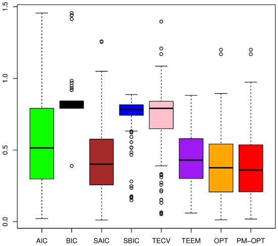
Figure 5.
Boxplots of ASEs under the guided semi-synthetic simulation based on the CPCRA dataset. Covariates and baseline outcomes are drawn from the real data, while the true HTEs are known. Lower is better.
In contrast, AIC and BIC exhibit higher median risks and wider spreads, especially for BIC, which tends to underfit in complex settings. The smoothed variants SAIC and SBIC yield moderate improvements over their classical counterparts, particularly in reducing variability, but still fall short of the performance attained by the targeted ensemble methods.
Overall, the evidence confirms that incorporating both model flexibility and treatment–covariate interactions, as done by PM–OPT, provides more robust and accurate estimation of HTEs in realistic settings.
To investigate the heterogeneity of treatment effects across baseline covariates, we visualize the estimated CATEs against two clinically relevant variables: age and baseline CD4 count. These variables represent respectively the patient’s immunological status and biological aging, both of which are known to moderate antiretroviral therapy response in HIV patients. We create two scatter plots (Figure 6), where each dot shows one individual. Each dot is colored by treatment group and positioned according to the individual’s estimated CATE.
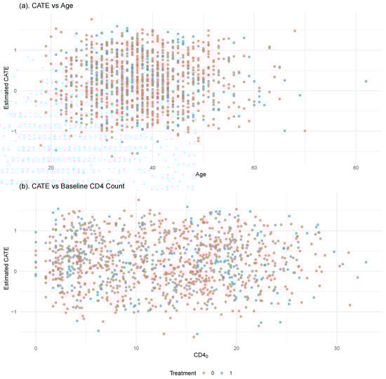
Figure 6.
Estimated CATEs from the PM-OPT method plotted against (a) patient age and (b) baseline CD4 cell count. Each point represents an individual, with color indicating treatment assignment (red: control, blue: treated). The CATE values quantify the estimated benefit of early Antiretroviral Therapy (ART) initiation for each individual.
Figure 6 displays the estimated CATEs as a function of patient age and baseline CD4 count. These CATEs are not derived from synthetic or simulated outcomes, but are instead estimated using the PM-OPT method based on the observed data in the CPCRA cohort. Overall, the CATE estimates are centered around zero, indicating no substantial average benefit or harm from early ART initiation in the full sample. This observation aligns with previous evidence showing that dual- and triple-drug regimens have comparable effects on CD4 counts at the population level ([37,38]).
Nevertheless, subtle heterogeneity is evident. Patients with lower baseline CD4 counts and those of younger age tend to show slightly more positive CATE estimates, suggesting a greater benefit from early treatment in these subgroups. These trends align with clinical intuition that younger individuals and those with weaker immune systems may respond more favorably to intensive ART. While the effects are not sharply pronounced, the PM-OPT estimator appears to capture meaningful variation in treatment response across individuals, underscoring its practical value in real-world data settings where the ground-truth treatment effect is unobservable.
6. Conclusions
This paper introduces a novel framework for estimating HTEs through model averaging combined with proximity-based matching. The proposed estimator, referred to as PMOPT, incorporates proximity information to construct pseudo-outcomes and employs a data-driven weighting scheme across candidate models. This approach enhances predictive accuracy and robustness across diverse scenarios. Comprehensive simulation studies and a guided empirical application show that the proposed method consistently outperforms traditional model selection methods, as well as several recent model averaging techniques, especially in settings characterized by nonlinear effects or treatment selection bias. Based on the numerical findings, PM–OPT consistently outperforms traditional model selection criteria in terms of accuracy and stability. PM–OPT achieves the lowest median errors and reduced variability, particularly in complex settings where treatment effects are heterogeneous or nonlinear. In contrast, AIC and BIC exhibit higher median risks and wider spreads, with BIC tending to underfit in more complex scenarios. While the smoothed variants SAIC and SBIC show moderate improvements in reducing variability, they still fall short of the performance attained by PM–OPT and OPT. It is particularly effective in moderate sample sizes, where model uncertainty is substantial and treatment heterogeneity is expected. These findings underscore the advantages of PM–OPT in handling more complex models and highlight its superior robustness and accuracy when faced with model uncertainty and HTEs.
While the empirical study demonstrates the utility of the proposed method in a realistic setting, we acknowledge some general limitations. First, as noted in Gao et al. [35], matching procedures, particularly those that rely on proximity scores, can become computationally intensive and may perform less reliably when sample sizes are small or the covariate space is high-dimensional. Second, similar to other observational methods, our approach relies on the assumption of no unmeasured confounding, an assumption that cannot be empirically verified. These considerations point to promising directions for future research, such as scalable approximate matching, incorporating domain knowledge, and sensitivity diagnostics, some of which we elaborate on below.
Moreover, although our theoretical framework relies on technical assumptions such as smooth response functions, compact covariate support, and uniform matching quality, these conditions are often only approximately satisfied in real-world applications. Nevertheless, our simulation results demonstrate that the proposed method remains effective even under moderate violations of such assumptions—for example, in scenarios with covariate imbalance or mild non-smoothness in treatment response surfaces.
In addition, as suggested in Gao et al. [35], the matching quality can be improved through domain-informed adjustments. Specifically, one may incorporate exact or near-exact matching constraints on important covariates or modify the proximity metric by penalizing key mismatches. These strategies can help maintain robustness when proximity learning is challenged by small sample sizes or high-dimensional covariate spaces. We regard the integration of such techniques and the development of adaptive matching diagnostics as important directions for future research.
Despite these promising results, our current analysis is restricted to low-dimensional linear regression models with binary treatment assignment. Several important directions remain open for future investigation. First, this paper focuses on low-dimensional settings, where model averaging theory is more mature. Extending PM-OPT to high-dimensional regimes is nontrivial, as the theoretical guarantees and asymptotic properties can differ significantly. Nevertheless, the proposed framework could potentially accommodate dimensionality reduction techniques (e.g., PCA or variable screening) and regularized base learners (e.g., Lasso or Ridge) to improve performance in high-dimensional applications. We leave these extensions as promising directions for future research. Second, adapting the method to generalized linear models, such as logistic or Poisson regression, could allow for broader use in binary or count outcome settings. Third, relaxing the binary treatment assumption to accommodate continuous, multi-valued, or dosage-type treatments would further generalize the framework to a wider range of causal inference problems. These extensions would require new theoretical developments and algorithmic strategies, but they hold the potential to further advance the flexibility and utility of proximity-informed model averaging in HTE estimation.
Finally, while several limitations have been discussed previously, including computational scalability, reliance on the unconfoundedness assumption, and the restriction to low-dimensional linear models, it is also important to note that the current framework assumes fully observed covariates. Extending the methodology to handle missing data, for example by applying imputation techniques or developing robust proximity measures, represents a valuable direction for future research.
Author Contributions
Conceptualization, Z.Z., L.Z. and Y.W.; Data curation, L.Z.; Formal analysis, Y.W.; Funding acquisition, Z.Z.; Investigation, L.Z.; Methodology, Z.Z.; Software, Z.Z.; Writing—original draft, Z.Z., L.Z. and Y.W. All authors will be updated at each stage of manuscript processing, including submission, revision, and revision reminder, via emails from our system or the assigned Assistant Editor. All authors have read and agreed to the published version of the manuscript.
Funding
This research was supported by the Youth Academic Innovation Team Construction Project of Capital University of Economics and Business (Grant No. QNTD202303), and by the Natural Science Foundation of Henan Province (Grant No. 252300420912).
Data Availability Statement
The data presented in this study are available on request from the corresponding author.
Conflicts of Interest
The authors declare no conflicts of interest.
Appendix A
Appendix A.1. Proof of Theorem 1
Proof.
Let and . Then
Next, consider
Using the Cauchy–Schwarz inequality,
Hence, by employing a line of reasoning similar to that used in the proof of (A.4) in [27],
Let , , , and .
From (12), we obtain the model average estimator
which yields
Let , and . From Assumption 4, we have
Then, we can obtain
and
Appendix A.2. Proof of Theorem 2
Proof.
The proof of Theorem 2 is based on the inequality results of [39] combined with Chebyshev’s inequality. For simplicity and in line with the proof of Theorem 2.1 in [40], we assume that the covariate matrix is non-random. This assumption is made without loss of generality, as all regularity conditions imposed on are satisfied almost surely, and thus the arguments extend to the stochastic case. In the subsequent proof, for ease of notation, we use C to denote generic constants that may differ from line to line.
Note that Condition (1) implies that
To establish (A14), we apply Condition (2) and Equation (A18), in conjunction with Chebyshev’s inequality and Theorem 2 of Whittle [39]. Following reasoning analogous to that used in Equation (A.1) of Wan et al. [19], we obtain, for any , that
Similarly, for (A15), we obtain
Now, to prove (A16), observe
We bound the first term
For the second term
Hence, condition (A16) is verified.
Now, to prove (A12), we first consider
Define the conditional risk
Denote the maximum singular value by . Following [19], we have
Recognizing that , we have
Now for the control projection matrix
Then
and
Additionally, we can show that
Similarly, we have
and
By the above results, it is readily seen that the right-hand side of (A23) converges to zero in probability.
Thus, (A11), (A12) and (A13) are proved, and this completes the proof of Theorem 2. □
Appendix B
Appendix B.1. Abbreviations
The following abbreviations are used throughout the paper
- HTE—Heterogeneous Treatment Effect
- CATE—Conditional Average Treatment Effect
- ATE—Average Treatment Effect
- PSM—Propensity Score Matching
- BIC—Bayesian Information Criterion
- AIC—Akaike Information Criterion
- JMA—Jackknife Model Averaging
- MMA—Mallows Model Averaging
- PM-OPT—Proximity Matching-based Optimal Averaging
- TECV—Treatment Effect Cross-Validation
- TEEM—Treatment Effect Estimation by Mixing
- SNR—Signal-to-Noise Ratio
- SUTVA—Stable Unit Treatment Value Assumption
Appendix B.2. Summary of Key Notation
Table A1.
Summary of key notation.
Table A1.
Summary of key notation.
| Symbol | Description |
|---|---|
| K | Number of candidate models |
| L | Number of matched pseudo-observation pairs (via combo matching) |
| Matched covariates in treated and control groups | |
| Matched outcomes in treated and control groups | |
| Predicted outcomes under model for treated/control units | |
| Projection matrices from full sample design matrices | |
| Projection matrices from matched sample design matrices | |
| Zero-padded projection matrices (aligned to length L) | |
| Weighted projection matrices: , . | |
| Model-averaged predicted outcomes for treated/control units | |
| Final model-averaged CATE estimator: | |
| Weight space: the unit simplex in | |
| Bias due to covariate imbalance: | |
| Composite noise term: |
Appendix B.3. The Algorithm of PM-OPT

References
- Ashenfelter, O. Estimating the Effect of Training Programs on Earnings. Rev. Econ. Stat. 1978, 60, 47–57. [Google Scholar] [CrossRef]
- LaLonde, R.J. Evaluating the Econometric Evaluations of Training Programs with Experimental Data. Am. Econ. Rev. 1986, 76, 604–620. [Google Scholar]
- Abadie, A.; Imbens, G.W. Bias-corrected Matching Estimators for Average Treatment Effects. J. Bus. Econ. Stat. 2011, 29, 1–11. [Google Scholar] [CrossRef]
- Imai, K.; Ratkovic, M. Estimating Treatment Effect Heterogeneity in Randomized Program Evaluation. Ann. Appl. Stat. 2013, 7, 443–470. [Google Scholar] [CrossRef]
- Wager, S.; Athey, S. Estimation and Inference of Heterogeneous Treatment Effects Using Random Forests. J. Am. Stat. Assoc. 2018, 113, 1228–1242. [Google Scholar] [CrossRef]
- Chipman, H.A.; George, E.I.; McCulloch, R.E. BART: Bayesian Additive Regression Trees. Ann. Appl. Stat. 2010, 4, 266–298. [Google Scholar] [CrossRef]
- Hill, J.L. Bayesian Nonparametric Modeling for Causal Inference. J. Comput. Graph. Stat. 2011, 20, 217–240. [Google Scholar] [CrossRef]
- Athey, S.; Imbens, G. Recursive Partitioning for Heterogeneous Causal Effects. Proc. Natl. Acad. Sci. USA 2016, 113, 7353–7360. [Google Scholar] [CrossRef]
- Raftery, A.E.; Madigan, D.; Hoeting, J.A. Bayesian Model Averaging for Linear Regression Models. J. Am. Stat. Assoc. 1997, 92, 179–191. [Google Scholar] [CrossRef]
- Hoeting, J.A.; Madigan, D.; Raftery, A.E.; Volinsky, C.T. Bayesian Model Averaging: A Tutorial. Stat. Sci. 1999, 14, 382–401. [Google Scholar] [CrossRef]
- Raftery, A.E.; Zheng, Y. Discussion: Performance of Bayesian Model Averaging. J. Am. Stat. Assoc. 2003, 98, 931–938. [Google Scholar] [CrossRef]
- Buckland, S.T. Model Selection: An Integral Part of Inference. Biometrics 1997, 53, 603–618. [Google Scholar] [CrossRef]
- Claeskens, G.; Hjort, N.L. The Focused Information Criterion. J. Am. Stat. Assoc. 2003, 98, 900–916. [Google Scholar] [CrossRef]
- Hjort, N.L.; Claeskens, G. Focused Information Criteria and Model Averaging for the Cox Hazard Regression Model. J. Am. Stat. Assoc. 2006, 101, 1449–1464. [Google Scholar] [CrossRef]
- Yang, Y. Adaptive Regression by Mixing. J. Am. Stat. Assoc. 2001, 96, 574–588. [Google Scholar] [CrossRef]
- Yang, Y. Regression with Multiple Candidate Models: Selecting or Mixing? Stat. Sin. 2003, 13, 783–809. [Google Scholar]
- Yang, Y. Combining Linear Regression Models: When and How? J. Am. Stat. Assoc. 2005, 100, 1202–1214. [Google Scholar] [CrossRef]
- Hansen, B.E. Least Squares Model Averaging. Econometrica 2007, 75, 1175–1189. [Google Scholar] [CrossRef]
- Wan, A.T.; Zhang, X.; Zou, G. Least Squares Model Averaging by Mallows Criterion. J. Econom. 2010, 156, 277–283. [Google Scholar] [CrossRef]
- Hansen, B.E.; Racine, J.S. Jackknife Model Averaging. J. Econom. 2012, 167, 38–46. [Google Scholar] [CrossRef]
- Zhang, X.; Zou, G.; Carroll, R.J. Model Averaging Based on Kullback-Leibler Distance. Stat. Sin. 2015, 25, 1583–1598. [Google Scholar] [CrossRef]
- Zhang, X.; Yu, D.; Zou, G.; Liang, H. Optimal Model Averaging Estimation for Generalized Linear Models and Generalized Linear Mixed-Effects Models. J. Am. Stat. Assoc. 2016, 111, 1775–1790. [Google Scholar] [CrossRef]
- Zhang, X.; Zou, G.; Liang, H.; Carroll, R.J. Parsimonious Model Averaging With a Diverging Number of Parameters. J. Am. Stat. Assoc. 2019, 115, 972–984. [Google Scholar] [CrossRef]
- Seng, L.; Li, J. Structural Equation Model Averaging: Methodology and Application. J. Bus. Econ. Stat. 2022, 40, 815–828. [Google Scholar] [CrossRef]
- Kitagawa, T.; Muris, C. Model Averaging in Semiparametric Estimation of Treatment Effects. J. Econom. 2016, 195, 358–368. [Google Scholar] [CrossRef]
- Rolling, C.A.; Yang, Y.; Velez, D. Combining Estimates of Conditional Treatment Effects. Econom. Theory 2019, 35, 1089–1110. [Google Scholar] [CrossRef]
- Zhao, Z.; Zhang, X.; Zou, G.; Wan, A.T.K.; Tso, G.K.F. Model Averaging for Estimating Treatment Effects. Ann. Inst. Stat. Math. 2024, 76, 73–92. [Google Scholar] [CrossRef]
- Rubin, D.B. Multivariate Matching Methods That Are Equal Percent Bias Reducing, I: Some Examples. Biometrics 1976, 32, 109–120. [Google Scholar] [CrossRef]
- Rubin, D.B. Bias Reduction Using Mahalanobis-Metric Matching. Biometrics 1980, 36, 293–298. [Google Scholar] [CrossRef]
- Rosenbaum, P.R.; Rubin, D.B. The Central Role of the Propensity Score in Observational Studies for Causal Effects. Biometrika 1983, 70, 41–55. [Google Scholar] [CrossRef]
- Rosenbaum, P.R.; Rubin, D.B. Reducing Bias in Observational Studies Using Subclassification on the Propensity Score. J. Am. Stat. Assoc. 1984, 79, 516–524. [Google Scholar] [CrossRef]
- Hansen, B.B. The Prognostic Analogue of the Propensity Score. Biometrika 2008, 95, 481–488. [Google Scholar] [CrossRef]
- Rosenbaum, P.R. A Characterization of Optimal Designs for Observational Studies. J. R. Stat. Soc. Ser. B Methodol. 1991, 53, 597–610. [Google Scholar] [CrossRef]
- Hansen, B.B. Full Matching in an Observational Study of Coaching for the SAT. J. Am. Stat. Assoc. 2004, 99, 609–618. [Google Scholar] [CrossRef]
- Gao, Z.; Hastie, T.; Tibshirani, R. Assessment of Heterogeneous Treatment Effect Estimation Accuracy via Matching. Stat. Med. 2021, 40, 3990–4013. [Google Scholar] [CrossRef] [PubMed]
- Lv, J.; Liu, J.S. Model Selection Principles in Misspecified Models. J. R. Stat. Soc. Ser. B Stat. Methodol. 2014, 76, 141–167. [Google Scholar] [CrossRef]
- Rolling, C.A.; Yang, Y. Model Selection for Estimating Treatment Effects. J. R. Stat. Soc. Ser. B Stat. Methodol. 2014, 76, 749–769. [Google Scholar] [CrossRef]
- MacArthur, R.D.; Novak, R.M.; Peng, G.; Chen, L.; Xiang, Y.; Hullsiek, K.H. A Comparison of Three Highly Active Antiretroviral Treatment Strategies Consisting of Non-Nucleoside Reverse Transcriptase Inhibitors, Protease Inhibitors, or Both in the Presence of Nucleoside Reverse Transcriptase Inhibitors as Initial Therapy (CPCRA 058 FIRST Study): A Long-Term Randomised Trial. Lancet 2006, 368, 2125–2135. [Google Scholar] [CrossRef] [PubMed]
- Whittle, P. Bounds for the Moments of Linear and Quadratic Forms in Independent Variables. Theory Probab. Appl. 1960, 5, 302–305. [Google Scholar] [CrossRef]
- Zhang, X.; Wan, A.T.; Zou, G. Model Averaging by Jackknife Criterion in Models with Dependent Data. J. Econom. 2013, 174, 82–94. [Google Scholar] [CrossRef]
Disclaimer/Publisher’s Note: The statements, opinions and data contained in all publications are solely those of the individual author(s) and contributor(s) and not of MDPI and/or the editor(s). MDPI and/or the editor(s) disclaim responsibility for any injury to people or property resulting from any ideas, methods, instructions or products referred to in the content. |
© 2025 by the authors. Licensee MDPI, Basel, Switzerland. This article is an open access article distributed under the terms and conditions of the Creative Commons Attribution (CC BY) license (https://creativecommons.org/licenses/by/4.0/).