Abstract
Multi-objective Unmanned Aerial Vehicle (UAV) path planning in complex 3D environments presents a fundamental challenge requiring the simultaneous optimization of conflicting objectives such as path length, safety, altitude constraints, and smoothness. This study proposes a novel hybrid framework, termed QL-MOPSO, that integrates reinforcement learning with metaheuristic optimization through a three-stage hierarchical architecture. The framework employs Q-learning to generate a global guidance path in a discretized 2D grid environment using an eight-directional symmetric action space that embodies rotational symmetry at π/4 intervals, ensuring uniform exploration capabilities and unbiased path planning. A crucial intermediate stage transforms the discrete 2D path into a 3D initial trajectory, bridging the gap between discrete learning and continuous optimization domains. The MOPSO algorithm then performs fine-grained refinement in continuous 3D space, guided by a novel Q-learning path deviation objective that ensures continuous knowledge transfer throughout the optimization process. Experimental results demonstrate that the symmetric action space design yields 20.6% shorter paths compared to asymmetric alternatives, while the complete QL-MOPSO framework achieves 5% path length reduction and significantly faster convergence compared to standard MOPSO. The proposed method successfully generates Pareto-optimal solutions that balance multiple objectives while leveraging the symmetry-aware guidance mechanism to avoid local optima and accelerate convergence, offering a robust solution for complex multi-objective UAV path planning problems.
1. Introduction
With the rapid advancement of unmanned aerial vehicle (UAV) technology, UAVs have found extensive applications across diverse domains, ranging from military operations to civilian services, including disaster monitoring, agriculture, environmental protection, infrastructure inspection, logistics delivery, urban planning, communication relay, and security patrol [1,2,3,4,5].
However, UAV path planning in complex three-dimensional environments presents significant challenges that extend far beyond simple point-to-point navigation. UAV path planning is inherently a multi-objective optimization problem involving several conflicting objectives that must be simultaneously optimized [6]. In real-world scenarios, UAVs must navigate through complex terrains while considering multiple criteria: minimizing flight distance to reduce energy consumption and mission time, ensuring flight safety by avoiding obstacles and threat zones, maintaining appropriate altitude to comply with airspace regulations and terrain constraints, and optimizing path smoothness to reduce mechanical stress and improve flight stability [7]. These objectives often conflict with each other—for instance, the shortest path may lead through high-threat areas, while the safest route might significantly increase flight distance and energy consumption [8].
The complexity of UAV path planning is further compounded by various constraints, including limited energy capacity, dynamic environmental conditions, real-time computational requirements, and regulatory restrictions. Traditional single-objective optimization approaches fail to adequately address these multifaceted requirements, as they cannot simultaneously balance competing objectives or provide decision-makers with a range of trade-off solutions. This limitation has driven the need for sophisticated multi-objective optimization techniques that can generate Pareto-optimal solutions, offering UAV operators flexibility in choosing paths based on mission-specific priorities [9].
Existing research in multi-objective UAV path planning has primarily focused on metaheuristic algorithms due to their ability to handle complex, high-dimensional, and nonlinear optimization problems [10,11,12]. Multi-objective particle swarm optimization (MOPSO) [13], non-dominated sorting genetic algorithm (NSGA) [14], multi-objective ant colony optimization (MOACO) [15,16], multi-objective grey wolf optimizer (MOGWO) [17], and multi-objective secretary bird optimization algorithm (IMOSBOA) [18] have been widely applied to UAV path planning with varying degrees of success.
Although the above-mentioned methods have been successfully applied to UAV path planning, a deeper analysis reveals that they struggle to holistically address the problem, often facing critical limitations.
Firstly, many existing methods grapple with the inherent conflict between global and local optimization. For instance, while algorithms like MOGWO [17] might identify a generally correct flight corridor (macro-scale planning), they often lack the mechanisms for fine-tuning the path for objectives like smoothness or minimal altitude variations (micro-scale refinement). This can result in paths that are globally feasible but locally suboptimal or inefficient. Our work addresses this by proposing a hierarchical framework that decouples these two conflicting demands.
Secondly, the performance of these swarm intelligence algorithms is highly sensitive to the quality of their initial population. Most studies, including [17,18,19], rely on random initialization. This “blind search” approach in the vast 3D solution space is inefficient, slows down convergence, and significantly increases the risk of getting trapped in local optima, failing to find a truly superior path. This limitation highlights the need for a mechanism to provide prior knowledge to guide the initial search, a core challenge our research tackles directly.
Thirdly, a significant gap exists in integrating knowledge from different learning paradigms. Recently, some studies have attempted to combine Reinforcement Learning (RL) with metaheuristics to improve performance [20]. However, a fundamental challenge remains: how to effectively transfer policy knowledge learned in a discrete, grid-based environment (typical for Q-learning [21,22,23]) to the continuous, real-world search space where UAV path planning truly operates. Existing approaches often lack a sophisticated bridging mechanism, leading to knowledge loss or ineffective guidance.
The integration of Q-learning into multi-objective optimization brings several key benefits:
- (1)
- Global path guidance: Q-learning can learn global navigation strategies by exploring the environment systematically, providing valuable guidance information about promising regions and paths to avoid [24]. This learned knowledge can significantly improve the initialization quality and search direction of population-based optimization algorithms.
- (2)
- Experience-based decision making: Unlike traditional random search methods, Q-learning builds a value function that captures the long-term reward expectations for different state–action pairs [25]. This knowledge can be transferred to guide the search process of metaheuristic algorithms, focusing exploration on high-potential regions.
- (3)
- Adaptive learning capability: Q-learning can continuously update its policy based on environmental feedback, making it particularly suitable for dynamic environments where conditions may change during mission execution [26].
- (4)
- Discrete-continuous space bridging: Q-learning naturally handles discrete state spaces, which can be effectively mapped to continuous optimization domains used by metaheuristic algorithms [27]. This bridging capability enables the integration of learned discrete policies with continuous path optimization.
- (5)
- Multi-scale optimization support: Q-learning can operate at different abstraction levels, learning both coarse-grained strategic policies and fine-grained tactical decisions [28]. This multi-scale capability complements the hierarchical nature of UAV path planning problems.
To address these specific shortcomings identified in the literature, this paper innovatively proposes a Q-learning guided multi-objective particle swarm optimization method for UAV 3D path planning (Q-Learning Guided MOPSO, QL-MOPSO). This method first positions reinforcement learning as a macro-level, strategic environmental learner, using Q-learning to quickly learn a global guiding path in a two-dimensional gridded environment. Then, this path and its value information are used as heuristic knowledge to guide MOPSO in performing refined and efficient multi-objective optimization in three-dimensional continuous space.
The main contributions of this article can be summarized as follows:
- (1)
- A Novel Three-Stage Hierarchical Planning Framework.
We propose a novel three-stage architecture that systematically decomposes the complex multi-objective path planning problem. This framework uniquely integrates a reinforcement learning agent for global route exploration (Stage 1) with a metaheuristic algorithm for local, fine-grained refinement (Stage 3). This hierarchical structure provides a robust and methodical solution to the inherent multi-scale challenges of UAV path planning.
- (2)
- A Discrete-to-Continuous Knowledge Transfer Mechanism.
We design and implement a crucial intermediate stage (Stage 2) that serves as a technical bridge between the discrete and continuous domains. This stage effectively transforms the 2D grid-based path knowledge acquired by Q-learning into a viable 3D initial trajectory. This mechanism explicitly solves the fundamental challenge of migrating learned policies from a discrete representation to a continuous optimization space.
- (3)
- A Knowledge-Guided Multi-Objective Optimization Model.
We enhance the standard MOPSO algorithm by introducing a novel, guidance-aware optimization objective, which we term “Q-learning Path Deviation”. By incorporating this deviation as a new objective in the fitness function, the framework ensures that the prior knowledge from the RL agent actively guides the entire search process—not just the initialization. This continuous guidance significantly improves convergence speed and the quality of the final Pareto-optimal solutions.
2. Materials and Methods
The QL-MOPSO method proposed in this paper follows a hierarchical, three-stage planning framework. Firstly (Stage 1), a Q-learning algorithm is employed to generate a global guidance path within a discretized 2D grid environment. Subsequently (Stage 2), this 2D path undergoes a crucial transformation and adaptation process, converting it into a viable initial trajectory in the 3D continuous space. Finally (Stage 3), a Multi-Objective Particle Swarm Optimization (MOPSO) algorithm performs a fine-grained refinement of this initial trajectory, simultaneously optimizing for conflicting objectives such as path length, flight safety, and energy consumption. The overall system framework is shown in Figure 1.
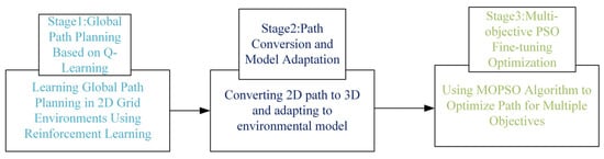
Figure 1.
Overall system framework.
The following sections will provide a detailed technical description of each of these stages.
2.1. Global Path Planning Based on Q-Learning
This stage aims to employ reinforcement learning methods to learn the optimal policy within a discretized state space, providing global guidance for subsequent path refinement and multi-objective optimization.
2.1.1. Environmental Modeling and State Space Definition
The two-dimensional environment where the UAV operates is abstracted as a discrete grid map. This map consists of M × N grid cells, as shown in Figure 2.
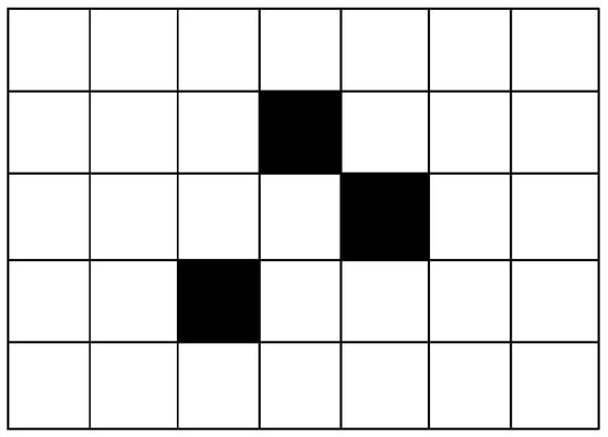
Figure 2.
Discrete grid map.
In Figure 2, we define the UAV’s location directly as its state. Therefore, each non-obstacle grid cell represents a unique state s that the UAV can occupy, and all such states collectively form the state space S, where .
Environmental information is stored in a two-dimensional matrix called “environment”, where each element represents the state of a grid cell. The value of a grid cell indicates whether that location is an obstacle: if environment (i,j) = 1, it means the cell is an obstacle that the drone cannot pass through (as shown in the black area in Figure 2); if it is 0, it indicates the cell is a free area that the drone can safely pass through.
2.1.2. Action Space Design and Symmetry Considerations
Considering the flexibility of drone movement in a 2D grid map and the symmetry of the environment, the action space A designed in this paper includes eight discrete actions A = {a1, a2, …, a8}. These actions correspond to the drone’s movement from its current state in the up, down, left, right, and four diagonal directions. This design embodies a rotational symmetry, where the action space, centered at the current state, exhibits symmetry at multiples of π/4 angles., as shown in Figure 3.
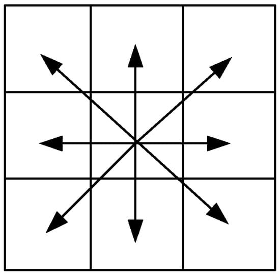
Figure 3.
Symmetry of Action Space.
The implementation of state transitions reflects this symmetry. Specifically, the process treats each state in the grid map as a two-dimensional coordinate and calculates the new coordinate based on the direction vector represented by the action. This design ensures that the drone has the same movement capability in all directions, avoiding path planning biases that could result from an unbalanced action space design. The state transition process must ensure that the newly calculated coordinates remain within the boundaries of the environment; if they exceed the environmental limits, the state remains unchanged.
2.1.3. Q-Learning Algorithm
The core of Q-learning is to create a Q-table, where each cell stores a Q (S, A) value, with S representing a state and A representing an action. Q (S, A) represents the value of taking a specific action in a given state, known as the action-value function [29]. The higher the action-value function, the more likely the agent will tend to take that action in that state. Conversely, if the value is lower, the agent is less likely to choose that action. By continuously training the agent with data and designing an appropriate reward function to guide it, a Q-table is ultimately generated. When solving problems, the system searches the Q-table using environmental data to find the corresponding state and selects the optimal action. Q-learning is an off-policy temporal difference reinforcement learning algorithm used to learn the value function of state-action pairs, namely the Q function Q (s, a). The structure of Q-learning is shown in Figure 4.
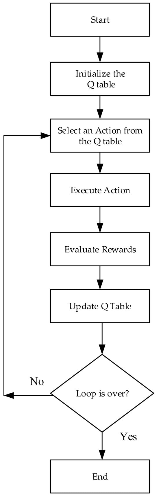
Figure 4.
The structure of Q-learning algorithm.
The update rule for Q-learning is as follows:
where represents the Q-value of executing action in state . is a learning rate; is the immediate reward obtained after executing action in state . is the discount factor used to balance the importance of immediate rewards and future rewards.
2.1.4. Reward Function Design
To guide the drone to learn a strategy that avoids obstacles and quickly reaches the target, the following reward function is designed:
where is set to a relatively large positive value, representing the reward for reaching the target state. is the penalty for hitting obstacles, typically set as a negative value. is the default reward in other states and is set to a relatively small negative value.
2.1.5. Optimal Path Extraction
After the Q-learning algorithm completes training, the optimal path is gradually constructed by starting from the initial state and selecting the action with the highest Q-value at each step until reaching the target state. This path serves as the guiding route for the UAV within the global environment and provides a reference for subsequent path optimization.
2.2. Path Conversion and Model Adaptation
The main objective of this phase is to convert the 2D global path generated by the Q-learning algorithm into an initial path in 3D space, and to construct an environmental model suitable for subsequent multi-objective optimization. This phase includes three key steps: two-dimensional path coordinate conversion, three-dimensional terrain model construction, and three-dimensional guidance path generation.
2.2.1. Two-Dimensional Path Coordinate Transformation
The Q-learning algorithm generates a global path represented by a series of grid cell indices. To facilitate subsequent 3D spatial path planning, these indices need to be converted into 2D coordinates. Specifically, assuming the optimal path generated by the Q-learning algorithm contains a series of linear indices of grid cells, by converting these linear indices to corresponding row coordinates (row) and column coordinates (col), we obtain the coordinates (rowi, coli) of each node on the path in the 2D grid map. The converted 2D path is represented as , where n is the number of path nodes.
2.2.2. Three-Dimensional Guidance Path Generation
To simulate a realistic 3D flight environment, it is necessary to build a 3D terrain model based on a 2D grid map. Then, the 2D path can be converted into a guidance path in 3D space. The specific implementation process is shown in Algorithm 1.
| Algorithm 1: 3D Guidance Path Generation |
| /*Input*/ Set 2D grid map environment_map, 2D path from Q-Learning path_2d, scaling factor scale_factor, and fixed flight altitude fixed_flight_altitude. /*Initialization*/ Initialize the height map H as an empty model. Initialize the threat list threats as an empty list. Set 3D map dimensions MAPSIZE_X, MAPSIZE_Y based on environment_map and scale_factor. Set map boundaries xmin, xmax, ymin, ymax, zmin, zmax. /*3D Terrain Model Construction*/ For each cell (i, j) in environment_map do Set base_height = Random value within a predefined range. If environment_map [i, j] == 1 do // Obstacle Area Set peak_center based on (i, j) and scale_factor. Generate a Gaussian surface centered at peak_center with base_height. Update the corresponding area in height map H. Define a spherical threat centered at peak_center and add to threats. Else // Free Area Generate a relatively flat surface with base_height and random noise. Update the corresponding area in height map H. End If End For /*3D Guidance Path Generation*/ Initialize guidance_path_3d as an empty path. For each node (r, c) in path_2d do Set x = r × scale_factor. Set y = c × scale_factor. Set z = fixed_flight_altitude. Append the 3D coordinate (x, y, z) to guidance_path_3d. End For /*Output*/ Output the initial 3D guidance path guidance_path_3d. Output the 3D terrain model H and the threat list threats. Output all map parameters for the next stage. |
2.3. Multi-Objective PSO Fine-Tuning Optimization
UAV trajectory planning requires combining multiple objective functions to evaluate the effectiveness of trajectory planning. These objective functions typically include a series of constraints and optimization conditions, with the goal of obtaining higher quality flight trajectories by minimizing the objective functions.
2.3.1. Multi-Objective Optimization Problem
A multi-objective optimization problem typically involves several conflicting objective functions [30,31]. The result is a set of trade-off solutions, known as the Pareto optimal solution set [32]. The corresponding set in the function space is called the Pareto front (PF). Mathematically, a multi-objective optimization problem can be expressed as
where fi(x) (i = 1, 2, …, k) is the objective function, and k is the number of objective functions.
The evaluation of solutions in Multi-Objective Optimization (MOO) is governed by the principle of Pareto Dominance. A solution x1 is said to dominate x2 if it is superior in at least one objective and not inferior in any of the others.
Solutions that are not dominated by any other solution within the search space are termed non-dominated or Pareto optimal. The collection of all such solutions forms the Pareto Optimal Set. This set represents the frontier of optimal trade-offs, as any improvement in one objective for a solution within this set requires a degradation in at least one other objective.
In algorithms like MOPSO, this set is dynamically maintained in an archive. These non-dominated solutions act as the leaders that guide the population’s search toward the Pareto Front, which is the projection of the Pareto Optimal Set in the objective space.
2.3.2. Constraints and Objective Functions
In the Multi-Objective Particle Swarm Optimization (MOPSO) algorithm, each particle represents a complete three-dimensional flight path. To evaluate the merit of each path, a comprehensive cost function is essential. This function quantifies various path performance metrics while considering diverse physical constraints. In this study, we consider the following four constraints: quantified path length, threat avoidance, flight altitude, and path smoothness.
So, the general multi-objective function f(x) from Equation (3) is specifically instantiated as a cost vector composed of four distinct objectives. The objective vector is formally defined as:
where x represents a complete 3D path.
The primary goal of the algorithm is to find a solution that minimizes this cost vector.
A path is defined by a start point , an end point , and n intermediate control points .The complete sequence of path points is , resulting in a total of N = n + 2 points. The definitions of the four sub-objective functions are detailed below.
- (1)
- Path Length Cost (J1)
This objective aims to find the shortest possible flight path to conserve mission time and energy. However, using the total path length directly is not ideal for normalization. Therefore, this study adopts the path’s “tortuosity” or “inefficiency” as the cost metric. Its mathematical expression is as follows:
where is the direct Euclidean distance between the start and end points (the shortest possible path), while the denominator is the actual flight path length. The more convoluted the path, the larger the denominator, and thus the larger the value of J1.
- (2)
- Threat Avoidance Cost (J2)
This objective measures the safety of the path, specifically its ability to maintain a safe standoff distance from known threats or obstacles. For each threat, a three-tiered cost is defined:
- Safe Zone: If the distance to the threat is greater than the sum of the threat radius, the drone’s size, and a predefined safety margin (danger_dist), the path is considered safe, and the cost is zero.
- Collision Zone: If the path enters the area defined by the threat radius plus the drone’s size, it is considered a collision. This violates a hard constraint, and the cost is set to infinity ().
- Danger Zone: If the path lies between the safe and collision zones, a penalty cost is incurred, which is proportional to the depth of the intrusion.
The total threat avoidance cost J2 is the average of all penalty costs over all path segments and threats:
The individual threat cost is given by
where d is the distance from the path segment to the threat’s center, and are the radius of the threat and drone, respectively, is the width of the danger zone, and .
- (3)
- Flight Altitude Cost (J3)
This objective is designed to maintain the UAV’s flight altitude within an optimal range, . This prevents collisions with the ground from flying too low and reduces exposure risk and energy consumption from flying too high. The cost function penalizes deviations from the median of the optimal altitude range.
where is the flight altitude of control point relative to the ground. If (a ground crash), the cost is set to infinity. This formulation normalizes the cost, yielding at the optimal median altitude and at the boundaries of the range.
- (4)
- Path Smoothness (J4)
This objective ensures the smoothness of the flight path by penalizing sharp turns, which is critical for the UAV’s maneuverability and energy efficiency. Smoothness is measured by calculating the change in heading angle at each turn point. The cost is the average of all normalized turning angles.
where the turning angle is calculated as the angle between two consecutive path segments:
where and are the vectors of the path segments meeting at point . The angle is normalized by dividing by π. A straighter path results in smaller angles and thus a lower cost J4.
2.3.3. The Modified MOPSO
We use the global guidance path generated in Stage 1 as expert knowledge to guide the MOPSO search process, ensuring both global optimality and local refinement. The core of this integration lies in how the knowledge from Q-learning is formally translated into guidance for the MOPSO. Specifically, the optimal path derived from the Q-learning stage, hereafter denoted as the “Q-learning Guidance Path” (PQL), is used to directly influence the MOPSO in two critical ways: guided population initialization and a guidance-enhanced velocity update mechanism. Furthermore, to ensure the refined path does not deviate excessively from the globally sound route provided by Q-learning, a new objective function, “Q-Learning Path Deviation”, is introduced.
- (1)
- Transformation of Q-Learning Knowledge into MOPSO Guidance
The knowledge extracted from the Q-learning stage is twofold:
- The Guidance Path (PQL): A sequence of 3D waypoints representing the optimal path found by the Q-learning agent. This path serves as a baseline for the MOPSO search.
- Guidance Strength (): A scalar hyperparameter that determines the magnitude of the Q-learning path’s influence on the optimization process.
- (2)
- Guided Population Initialization
A purely random initialization of the MOPSO population can lead to slow convergence. To accelerate the search process by starting in a promising region of the solution space, a portion of the initial population is generated based on the Q-learning Guidance Path. During the population initialization phase, a predefined fraction of particles (e.g., 33%) are initialized not as random paths, but as stochastic variations of (PQL).
- (3)
- The modified velocity update approach guided by Q-learning
The standard MOPSO velocity update calculates a particle’s new velocity based on its personal best (pbest) and the swarm’s global best (gbest, or a leader from the Pareto archive), which can be shown as Equation (11).
where is the inertia weight. c1, c2 are the acceleration coefficients for the cognitive, social, and guidance components, respectively. r1, r2 are random numbers in [0, 1]. is the current position of the particle. is the particle’s personal best position. is the position of the selected leader from the Pareto archive.
To establish an explicit guidance mechanism, we incorporate the Q-learning knowledge directly into the particle’s velocity update rule. So, we extend this formula by adding a third term, the “Q-Learning Guidance Term”, which attracts the particle towards the Q-learning path PQL.
The modified velocity update equation for the d-th dimension of particle I at time step t is
where c3 is the guidance coefficient, a new parameter that controls the strength of the Q-learning path’s attraction. r3 are random numbers in [0, 1]. is the corresponding dimensional component from the Q-learning Guidance Path.
- (4)
- “Q-Learning Path Deviation” Objective Function
To explicitly manage the trade-off between adhering to the Q-learning path and optimizing other objectives, we introduce a fifth objective function, J5 (Q-Learning Path Deviation). This objective quantifies how much a candidate path generated by MOPSO, PPSO, deviates from the Q-learning guidance path, PQL
It is formulated as the average Euclidean distance between the corresponding waypoints of the two paths:
where N is the number of waypoints, is the k-th waypoint of the candidate PSO path, and is the k-th waypoint of the Q-learning guidance path.
This new objective is added to the existing set of objectives. The full objective vector to be minimized by MOPSO is now modified as follows:
This objective is handled like any other within the MOPSO framework, contributing to the Pareto dominance calculations and influencing which solutions are kept in the external archive.
Summarizing the above, the specific implementation procedure of MOPSO fine-tuning optimization can be shown in Algorithm 2.
| Algorithm 2: Multi-objective PSO fine-tuning optimization |
| /*Input*/ Set maximum number of iterations t_max. Set population size NP, external archive capacity nRep. Set PSO parameters: inertia weight w, damping ratio w_damp. Set mutation probability p_mutation. Input the guidance path from Stage 1: Path_2D_guided. /*Initialization*/ Set the generation number t = 1. For each particle i = 1 to NP do If i <= NP/3 then // Guided Initialization Initialize particle position P_i based on Path_2D_guided with random perturbation. Else// Random Initialization Initialize particle position P_i randomly within the solution space. End If Initialize particle velocity v_i = 0. Evaluate the objective vector Cost(P_i) with Equation (4) Initialize the personal best position pbest_i = P_i. End For Establish External Archive /*Iteration Computation*/ While t < t_max do For each particle i = 1 to NP do Select a leader P_leader from the archive Calculate the guidance strength γ which decays with iteration t. Update velocity v_i based on w, pbest_i, P_leader, and the influence of Path_2D_guided controlled by γ. Update particle position P_i = P_i + v_i. If rand < p_mutation then Perform mutation operation on P_i. End If Evaluate the new objective vector Cost(P_i). If Cost(P_i) dominates Cost(pbest_i) then pbest_i = P_i. End If End For Update the external archive t = t + 1 End While /*Output*/ Select the final solution Path_final from the external archive based on specific user criteria. Output the optimal path Path_final for the UAV. |
3. Experimental Simulation and Result Analysis
3.1. Experimental Setup
To evaluate the effectiveness of QL-MOPSO, we conducted a series of experiments under different conditions. These experiments were conducted on a desktop PC with a 3.20 GHz CPU and 32 GB memory, using software such as Windows 10 and MATLAB 2022b. The parameter settings for Q-learning and MOPSO are shown in Table 1. These parameters were determined based on preliminary experiments and common practices in the reinforcement learning literature.

Table 1.
Some parameter settings for Q-learning and MOPSO.
3.2. Validation of the Symmetric Action Set in QL-MOPSO
To validate the critical role of symmetry in the agent’s decision-making process, a comparative experiment was designed. This experiment aims to investigate whether a symmetric action space (i.e., eight directions) provides a tangible advantage over an asymmetric one for the quality of the final 3D path. The hypothesis is that a symmetric set allows for more uniform exploration and generates a less biased, higher-quality guidance path for the subsequent MOPSO stage.
The experimental setup for validating action space symmetry involved two scenarios. The first, our proposed Symmetric model, employs an eight-direction action set (cardinal and diagonal). The second, a comparative Asymmetric model, is limited to a four-direction set (cardinal only), creating an anisotropic search bias. Crucially, all other algorithmic parameters for both the Q-learning and MOPSO modules were kept identical to isolate the variable of action space structure. The results of the comparative experiment are shown in Table 2 and Figure 5.
Table 2.
Symmetric approach vs. asymmetric approach.
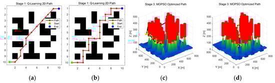
Figure 5.
Symmetric approach vs. asymmetric approach: (a) 2D path by eight actions; (b) 2D path by four actions; (c) 3D path by four actions; (d) 3D path by eight actions. The red zone is a threat area.
From Table 2 and Figure 5, we can see the experimental results confirm that the symmetric eight-action agent significantly outperforms its four-action counterpart. It produced a 20.6% shorter final path and achieved superior Pareto cost values, particularly for path length and flight objectives. The results reveal a clear trade-off. While not achieving strict Pareto dominance, the symmetric approach yields a solution with compelling advantages in mission-critical objectives, demonstrating a 53.4% reduction in Path Length Cost (J1) and a 37.9% reduction in Flight Altitude Cost (J3). This significant gain comes at the cost of a comparatively minor concession in path smoothness (J4).
This performance gain is attributed to a more efficient initial guidance path (12 steps vs. 19 steps) and was achieved at a negligible difference in computational cost. This validates that a symmetric action space is critical for guiding the hybrid algorithm toward a higher-quality solution.
3.3. Parameter Sensitivity Analysis
To validate the robustness of the proposed algorithm and the parameter settings presented in Table 3, we conducted a comprehensive sensitivity analysis. This analysis systematically investigates the impact of three key Q-learning parameters—the learning rate (α), the discount factor (γ), and the initial exploration rate (ε)—on the guide path length (steps) planning performance. For each parameter test, one parameter was varied across a predefined range while the others were held constant at their original values as specified in Table 3. To ensure statistical reliability, each parameter setting was independently run 30 times, and the mean and standard deviation of the resulting optimal path length were recorded. The parameters for the MOPSO component were set to standard, widely used values from established literature, which are known to be robust. The results are presented in Figure 6.
Table 3.
Comparative Results of Different Algorithms over 30 Independent Runs.
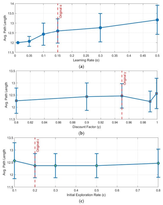
Figure 6.
Parameter Sensitivity Analysis. (a) Effect of Learning Rate on Path Length, (b) Effect of Discount Factor on Path Length, (c) Effect of Initial Exploration Rate (ε) on Path Length.
From the Figure 5, we have the following findings:
- (1)
- Learning Rate (α): The model exhibits low sensitivity to α. While lower values (e.g., 0.01) yield marginally shorter paths, our chosen value of 0.15 resides in a region of high stability, offering a robust balance between performance and convergence speed.
- (2)
- Discount Factor (γ): The algorithm is highly robust to variations in γ. Across the tested range of [0.8, 0.999], path length and stability remained consistently excellent, confirming that our choice of 0.95 lies within the optimal performance plateau.
- (3)
- Exploration Rate (ε): A clear optimal range for ε was identified between 0.2 and 0.5. Our selection of ε = 0.2 is empirically validated, as it ensures sufficient exploration to find the optimal path without being hampered by excessive randomness.
3.4. Comparative Performance Analysis
To rigorously evaluate the effectiveness and competitiveness of the proposed QL-MOPSO algorithm, we conducted a comprehensive comparative analysis against the following several state-of-the-art or classical optimization algorithms: the original MOPSO, NSGA-II, MOGWO, and Differential Evolution (DE). All algorithms were executed within the same simulated environment and tasked with the same path planning problem. To save running time, all algorithms used a population size of 80 and 300 iterations.
3.4.1. Experimental Results
To ensure statistical validity, each algorithm was independently run 30 times. The performance was evaluated based on three primary metrics: Optimization Time (computational efficiency), Final Composite Cost (solution quality based on the problem’s objective function), and 3D Path Length (the most direct measure of path quality). Furthermore, the Success Rate of finding a feasible solution was recorded to evaluate algorithm robustness. The aggregated results, presented as mean ± standard deviation, are recorded in Table 3 and Figure 7.
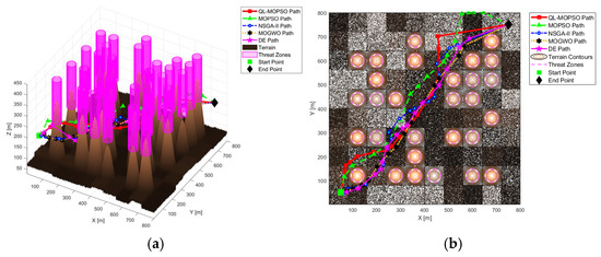
Figure 7.
A visual comparison of the optimal paths generated by each algorithm. (a) 3D Path Comparison Overview, (b) 2D Path Comparison (Top-Down View).
3.4.2. Analysis of Experimental Results
From Table 3, we can make the following key observations:
- (1)
- Superior Path Quality: QL-MOPSO achieves the best performance in the most critical metric, delivering the shortest average path length (1234.57 m). Its significantly lower standard deviation (55.41) also confirms its superior consistency over all competitors.
- (2)
- High Reliability and Efficiency: It demonstrates excellent robustness with a 100% success rate, unlike NSGA-II, which was highly unreliable (60% success). This reliability is achieved with no significant computational penalty, running faster than MOPSO and competitively with MOGWO.
- (3)
- Computational Efficiency: Our QL-MOPSO (32.21 s) and MOGWO (32.11 s) showed nearly identical and highly competitive computational times. Notably, the Q-learning guidance mechanism did not introduce a significant computational burden, as QL-MOPSO was even slightly faster than the MOPSO (35.56 s).
- (4)
- Strategic Cost Trade-off: While MOGWO registered a lower composite cost, this reflects our algorithm’s successful design. QL-MOPSO is intentionally focused on prioritizing geometric path minimization, and it excels in this primary objective, accepting a calculated trade-off in other, secondary cost functions.
- (5)
- Best Results Display: Figure 7 displays the single best path achieved by each algorithm across all 30 experimental runs, illustrating their optimal-case performance. Visually, the path from MOGWO (black stars) appears to be the most geometrically efficient in this best-case scenario. However, this observation must be contextualized by the aggregated statistical data in Table 3, which reveals a more nuanced conclusion.
The exceptional MOGWO path in the figure is the product of a high-risk search strategy. This strategy attempts to find shortcuts by navigating extremely close to threat zones, a gamble that can occasionally yield a very short path but is not consistently effective, as shown by its poorer average performance. This is evidenced by MOGWO’s significantly worse average path length (1265.96 m) and much larger standard deviation (100.20) over the 30 trials.
3.4.3. Summary of Comparison
In conclusion, the comparative analysis demonstrates the clear advantages of the proposed QL-MOPSO algorithm. While some algorithms may show superior performance in an isolated, secondary metric (e.g., MOGWO in composite cost), QL-MOPSO provides the best overall and balanced performance profile for the path planning task. It consistently finds the shortest paths among all tested methods, while demonstrating high reliability (100% success rate) and competitive computational speed. The results empirically validate that the integration of the Q-learning guidance mechanism effectively enhances the exploration and exploitation capabilities of MOPSO, elevating its performance beyond that of several other well-regarded optimization algorithms.
3.5. Ablation Analysis of the Q-Learning Path Deviation Term in MOPSO Fitness
In this section, we have performed an ablation study to isolate and analyze the impact of the Q-learning path deviation term. To achieve this, we created a “baseline” version of our algorithm by ablating the Q-learning component. We compared the performance of two models:
- (1)
- Full QL-MOPSO (five objectives): Our complete model, which utilizes Q-learning for (a) guided initialization, (b) guided velocity updates, and (c) the J5 path deviation objective.
- (2)
- Ablated QL-MOPSO (four objectives): This model is identical to the full model in every way, including using Q-learning for guided initialization and velocity updates, but we removed the J5 objective from the fitness evaluation.
Both algorithms were run 30 times on the same set of test scenarios used in the manuscript to ensure a fair and statistically significant comparison. The results are recorded in Table 4.
Table 4.
Ablation Analysis over 30 Independent Runs.
From Table 4, we can see that the “Q-Learning Path Deviation” (J5) objective is a critical component of the QL-MOPSO algorithm. The full QL-MOPSO model produced paths that were 6.8% shorter on average than the ablated version (1234.57 vs. 1325.76). This directly demonstrates that the J5 objective effectively guides the search towards superior solutions. Furthermore, the standard deviation in path length for the full model was nearly half that of the ablated model (55.41 vs. 132.82), indicating significantly more reliable and consistent performance.
4. Discussion
This section first discusses the central finding regarding the impact of action space geometry, then acknowledges the study’s limitations and outlines a clear roadmap for future research, incorporating the valuable feedback from the reviewers.
4.1. The Critical Role of Action Space Geometry in Guidance Quality
A key finding of this work is the critical impact of action space geometry on guidance path quality. The conventional four-direction action space imposes a strong anisotropic bias, forcing inefficient “staircase” maneuvers that are artifacts of the grid. In contrast, our symmetric eight-direction model facilitates more isotropic (directionally uniform) exploration, allowing the agent to discover paths that are more faithful abstractions of true Euclidean trajectories. This high-fidelity guidance, evidenced by a 20.6% path length reduction, is fundamental to our framework’s success. It directly leads to the accelerated convergence and superior Pareto-front solutions of QL-MOPSO, validating the principle that the integrity of the problem abstraction is paramount in hierarchical optimization.
4.2. Limitations and Future Directions
Building on these findings, we also acknowledge the limitations of the current study and outline a path for future work.
- (1)
- Performance in Dynamic and Real-World Scenarios: The most critical future direction is bridging the sim-to-real gap. Future work will extend the framework to handle dynamic environments, likely by using the trained Q-table as a “warm start” for rapid re-planning. Subsequently, we plan a staged validation process, including hardware-in-the-loop (HIL) simulations and field tests on a physical UAV platform, to assess the algorithm’s robustness against real-world uncertainties.
- (2)
- Scalability and Algorithmic Enhancements: Further research will analyze the scalability of QL-MOPSO in larger, more complex environments to understand its computational limits. To handle continuous state spaces more directly and potentially improve scalability, we also plan to explore replacing tabular Q-learning with Deep Reinforcement Learning (DRL) techniques.
- (3)
- Reward Function and Path Biases:
The reward function in our Q-learning model was designed for simplicity and robustness, prioritizing goal achievement while penalizing collisions and path length. We recognize this design has inherent limitations. Specifically, the uniform step penalty biases the agent towards the geometrically shortest path, which may not always be the safest. Furthermore, the binary penalty for obstacles prevents the model from assessing varying levels of threat, treating all navigable areas as equally safe. Future research could focus on developing more sophisticated, non-linear reward functions that incorporate risk gradients (e.g., proximity to threats) and utilize reward shaping techniques to improve learning efficiency and generate paths that are optimal not only in length but also in safety and robustness.
- (4)
- Adaptation to Real-World Terrain and Dynamic Obstacles:
In Section 2.2, we utilized a synthetically generated terrain model and assumed a static environment for the initial 2D path planning phase. We acknowledge that this is a simplification.
Real-World Terrain Integration: For direct application with real-world geographical data, the terrain generation step in Algorithm 1 would be replaced by importing a Digital Elevation Model (DEM). The `fixed_flight_altitude` parameter would then need to be interpreted as an altitude above the terrain data, requiring a more sophisticated altitude adaptation mechanism rather than a fixed value. This would involve ensuring the UAV maintains a safe minimum altitude over varying ground levels, which would be a valuable extension of our work.
Handling Moving Obstacles: The current QL-MOPSO framework does not explicitly account for moving obstacles within its 2D-to-3D path transformation. The Q-learning stage generates a globally optimal path based on a static threat map. Addressing dynamic threats would require significant architectural extensions, such as integrating a real-time perception and re-planning module. For example, the initial global path from QL-MOPSO could serve as a baseline, with a local, real-time planner (like Dynamic Window Approach or a lightweight RL agent) responsible for reactive collision avoidance. This hierarchical approach, where our method provides the global strategy and another component handles local tactics, is a promising direction for future research.
By explicitly outlining these aspects, we clarify the current scope of our algorithm and establish a clear and robust roadmap for future research that will further enhance the practical applicability of the QL-MOPSO framework. This structured roadmap addresses the current limitations and sets a clear path for research that will further solidify the practical value of the QL-MOPSO framework.
5. Conclusions
This study introduced QL-MOPSO, a novel hybrid framework that integrates Q-learning with multi-objective particle swarm optimization for 3D UAV path planning. Our central innovation was a rotationally symmetric action space that ensures high-fidelity global path guidance, which in turn seeds the 3D optimizer.
Comparative simulations demonstrated clear advantages. The framework’s core principles—geometric integrity and knowledge-guided optimization—led to significantly shorter paths, faster convergence, and superior Pareto fronts for trade-off objectives compared to baseline methods. The results confirm that hierarchically integrating reinforcement learning with swarm intelligence is a robust strategy for solving complex, multi-objective navigation problems.
While the framework shows great promise, we acknowledge its current limitations, primarily its validation within static environments and simplifications in the underlying models. As detailed in the Discussion, future work will focus on bridging the sim-to-real gap by addressing dynamic scenarios, enhancing algorithmic scalability, and conducting physical hardware validation.
In conclusion, the QL-MOPSO framework represents a significant step toward developing more intelligent and efficient autonomous navigation systems. It validates the power of hybrid, knowledge-guided strategies and opens new avenues for future research in the field.
Author Contributions
Conceptualization, W.L. and Q.X.; methodology, W.L. and Y.X.; software, W.L. and Y.X.; validation, W.L. and Y.X.; formal analysis, Y.X.; investigation, Y.X.; resources, Q.X.; data curation, W.L.; writing—original draft preparation, W.L. and Y.X.; writing—review and editing, W.L. and Y.X.; visualization, Y.X.; supervision, Q.X.; project administration. Y.X.; funding acquisition, W.L. All authors have read and agreed to the published version of the manuscript.
Funding
This work was partially supported by the Natural Science Foundation of Hunan Province under Grant No. 2025JJ70706; the Doctoral Research Start-up Fund Project of Hunan University of Arts and Science (NO. 25BSQD07).
Data Availability Statement
Data are contained within the article.
Conflicts of Interest
The authors declare no conflicts of interest.
Abbreviations
The following abbreviations are used in this manuscript:
| UAV | Unmanned Aerial Vehicle |
| MOPSO | Multi-Objective Particle Swarm Optimization (MOPSO) |
| QL-MOPSO | Q-Learning based MOPSO |
| NSGA | non-dominated sorting genetic algorithm |
| MOACO | multi-objective ant colony optimization |
| MOGWO | multi-objective grey wolf optimizer |
| RL | Reinforcement Learning |
| MOO | Multi-Objective Optimization |
References
- Yang, Y.; Fu, Y.; Xin, R.; Feng, W.; Xu, K. Multi-UAV Trajectory Planning Based on a Two-Layer Algorithm Under Four-Dimensional Constraints. Drones 2025, 9, 471. [Google Scholar] [CrossRef]
- Chen, H.; Liang, Y.; Meng, X. A UAV Path Planning Method for Building Surface Information Acquisition Utilizing Opposition-Based Learning Artificial Bee Colony Algorithm. Remote Sens. 2023, 15, 4312. [Google Scholar] [CrossRef]
- Lv, F.; Jian, Y.; Yuan, K.; Lu, Y. Unmanned Aerial Vehicle Path Planning Method Based on Improved Dung Beetle Optimization Algorithm. Symmetry 2025, 17, 367. [Google Scholar] [CrossRef]
- Haidar Ahmad, A.; Zahwe, O.; Nasser, A.; Clement, B. Path Planning for Unmanned Aerial Vehicles in Dynamic Environments: A Novel Approach Using Improved A* and Grey Wolf Optimizer. World Electr. Veh. J. 2024, 15, 531. [Google Scholar] [CrossRef]
- Li, W.; Zhang, K.; Xiong, Q.; Chen, X. Three-Dimensional Unmanned Aerial Vehicle Path Planning in Simulated Rugged Mountainous Terrain Using Improved Enhanced Snake Optimizer (IESO). World Electr. Veh. J. 2025, 16, 295. [Google Scholar] [CrossRef]
- Güven, İ.; Yanmaz, E. Multi-objective path planning for multi-UAV connectivity and area coverage. Ad Hoc Netw. 2024, 160, 103520. [Google Scholar] [CrossRef]
- Zhang, W.; Peng, C.; Yuan, Y.; Cui, J.; Qi, L. A novel multi-objective evolutionary algorithm with a two-fold constraint-handling mechanism for multiple UAV path planning. Expert Syst. Appl. 2024, 238, 121862. [Google Scholar] [CrossRef]
- Xu, X.; Xie, C.; Luo, Z.; Zhang, C.; Zhang, T. A multi-objective evolutionary algorithm based on dimension exploration and discrepancy evolution for UAV path planning problem. Inf. Sci. 2024, 657, 119977. [Google Scholar] [CrossRef]
- Petchrompo, S.; Coit, D.W.; Brintrup, A.; Wannakrairot, A.; Parlikad, A.K. A review of Pareto pruning methods for multi-objective optimization. Comput. Ind. Eng. 2022, 167, 108022. [Google Scholar] [CrossRef]
- Yahia, H.S.; Mohammed, A.S. Path planning optimization in unmanned aerial vehicles using meta-heuristic algorithms: A systematic review. Environ. Monit. Assess. 2023, 195, 30. [Google Scholar] [CrossRef]
- Hooshyar, M.; Huang, Y.M. Meta-heuristic algorithms in UAV path planning optimization: A systematic review (2018–2022). Drones 2023, 7, 687. [Google Scholar] [CrossRef]
- Wu, Y.; Liang, T.; Gou, J.; Tao, C.; Wang, H. Heterogeneous mission planning for multiple UAV formations via metaheuristic algorithms. IEEE Trans. Aerosp. Electron. Syst. 2023, 59, 3924–3940. [Google Scholar] [CrossRef]
- Xia, S.; Zhang, X. Constrained path planning for unmanned aerial vehicle in 3D terrain using modified multi-objective particle swarm optimization. Actuators 2021, 10, 255. [Google Scholar] [CrossRef]
- Ma, H.; Zhang, Y.; Sun, S.; Liu, T.; Shan, Y. A comprehensive survey on NSGA-II for multi-objective optimization and applications. Artif. Intell. Rev. 2023, 56, 15217–15270. [Google Scholar] [CrossRef]
- Awadallah, M.A.; Makhadmeh, S.N.; Al-Betar, M.A.; Dalbah, L.M.; Al-Redhaei, A.; Kouka, S.; Enshassi, O.S. Multi-objective ant colony optimization. Arch. Comput. Methods Eng. 2025, 32, 995–1037. [Google Scholar] [CrossRef]
- Ntakolia, C.; Lyridis, D.V. A comparative study on Ant Colony Optimization algorithm approaches for solving multi-objective path planning problems in case of unmanned surface vehicles. Ocean. Eng. 2022, 255, 111418. [Google Scholar] [CrossRef]
- Makhadmeh, S.N.; Alomari, O.A.; Mirjalili, S.; Al-Betar, M.A.; Elnagar, A. Recent advances in multi-objective grey wolf optimizer, its versions and applications. Neural Comput. Appl. 2022, 34, 19723–19749. [Google Scholar] [CrossRef]
- Tang, R.; Qi, L.; Ye, S.; Li, C.; Ni, T.; Guo, J.; Liu, H.; Li, Y.; Zuo, D.; Shi, J.; et al. Three-Dimensional Path Planning for AUVs Based on Interval Multi-Objective Secretary Bird Optimization Algorithm. Symmetry 2025, 17, 993. [Google Scholar] [CrossRef]
- Xiong, Q.; Zhang, X.; He, S.; Shen, J. A fractional-order chaotic sparrow search algorithm for enhancement of long distance iris image. Mathematics 2021, 9, 2790. [Google Scholar] [CrossRef]
- Zhang, X.; Xia, S.; Li, X.; Zhang, T. Multi-objective particle swarm optimization with multi-mode collaboration based on reinforcement learning for path planning of unmanned air vehicles. Knowl.-Based Syst. 2022, 250, 109075. [Google Scholar] [CrossRef]
- Zheng, F. Research on robot motion state estimation based on deep reinforcement learning. J. Hunan Univ. Arts Sci. (Nat. Sci.) 2023, 35, 34–39. [Google Scholar]
- Lyu, L.; Shen, Y.; Zhang, S. The advance of reinforcement learning and deep reinforcement learning. In Proceedings of the IEEE International Conference on Electrical Engineering, Big Data and Algorithms (EEBDA), Changchun, China, 25–27 February 2022; IEEE: New York, NY, USA, 2022; pp. 644–648. [Google Scholar]
- Puente-Castro, A.; Rivero, D.; Pedrosa, E.; Pereira, A.; Lau, N.; Fernandez-Blanco, E. Q-learning based system for path planning with unmanned aerial vehicles swarms in obstacle environments. Expert Syst. Appl. 2024, 235, 121240. [Google Scholar] [CrossRef]
- Souto, A.; Alfaia, R.; Cardoso, E.; Araújo, J.; Francês, C. UAV Path Planning Optimization Strategy: Considerations of Urban Morphology, Microclimate, and Energy Efficiency Using Q-Learning Algorithm. Drones 2023, 7, 123. [Google Scholar] [CrossRef]
- Sonny, A.; Yeduri, S.R.; Cenkeramaddi, L.R. Q-learning-based unmanned aerial vehicle path planning with dynamic obstacle avoidance. Appl. Soft Comput. 2023, 147, 110773. [Google Scholar] [CrossRef]
- Wu, J.; Sun, Y.; Li, D.; Shi, J. An adaptive conversion speed Q-learning algorithm for search and rescue UAV path planning in unknown environments. IEEE Trans. Veh. Technol. 2023, 72, 15391–15404. [Google Scholar] [CrossRef]
- Wang, L.; Zhang, L.; Liu, Y.; Wang, Z. Extending Q-learning to continuous and mixed strategy games based on spatial reciprocity. Proc. R. Soc. A 2023, 479, 20220667. [Google Scholar] [CrossRef]
- Mirzanejad, M.; Ebrahimi, M.; Vamplew, P.; Veisi, H. An online scalarization multi-objective reinforcement learning algorithm: TOPSIS Q-learning. Knowl. Eng. Rev. 2022, 37, e7. [Google Scholar] [CrossRef]
- Zhao, S.; Wu, Y.; Tan, S.; Wu, J.; Cui, Z.; Wang, Y.-G. QQLMPA: A quasi-opposition learning and Q-learning based marine predators algorithm. Expert Syst. Appl. 2023, 213, 119246. [Google Scholar] [CrossRef]
- Sharma, S.; Kumar, V. A comprehensive review on multi-objective optimization techniques: Past, present and future. Arch. Comput. Methods Eng. 2022, 29, 5605–5633. [Google Scholar] [CrossRef]
- Pereira, J.L.J.; Oliver, G.A.; Francisco, M.B.; Cunha, S.S.; Gomes, G.F. A review of multi-objective optimization: Methods and algorithms in mechanical engineering problems. Arch. Comput. Methods Eng. 2022, 29, 2285–2308. [Google Scholar] [CrossRef]
- Dosantos, P.S.; Bouchet, A.; Mariñas-Collado, I.; Montes, S. OPSBC: A method to sort Pareto-optimal sets of solutions in multi-objective problems. Expert Syst. Appl. 2024, 250, 123803. [Google Scholar] [CrossRef]
Disclaimer/Publisher’s Note: The statements, opinions and data contained in all publications are solely those of the individual author(s) and contributor(s) and not of MDPI and/or the editor(s). MDPI and/or the editor(s) disclaim responsibility for any injury to people or property resulting from any ideas, methods, instructions or products referred to in the content. |
© 2025 by the authors. Licensee MDPI, Basel, Switzerland. This article is an open access article distributed under the terms and conditions of the Creative Commons Attribution (CC BY) license (https://creativecommons.org/licenses/by/4.0/).