Abstract
Fractional-order chaotic systems have emerged as powerful tools in secure communications and multimedia protection owing to their memory-dependent dynamics, large key spaces, and high sensitivity to initial conditions. However, most existing fractional-order image encryption schemes rely on fixed-order chaos and conventional solvers, which limit their complexity and reduce unpredictability, while also neglecting the potential of variable fractional-order (VFO) dynamics. Although similar phenomena have been reported in some fractional-order systems, the coexistence of hidden attractors and stable equilibria has not been extensively investigated within VFO frameworks. To address these gaps, this paper introduces a novel discrete variable fractional-order dark matter–dark energy (VFODM-DE) chaotic system. The system is discretized using the piecewise constant argument discretization (PWCAD) method, enabling chaos to emerge at significantly lower fractional orders than previously reported. A comprehensive dynamic analysis is performed, revealing rich behaviors such as multistability, symmetry properties, and hidden attractors coexisting with stable equilibria. Leveraging these enhanced chaotic features, a pseudorandom number generator (PRNG) is constructed from the VFODM-DE system and applied to grayscale image encryption through permutation–diffusion operations. Security evaluations demonstrate that the proposed scheme offers a substantially large key space (approximately ) and exceptional key sensitivity. The scheme generates ciphertexts with nearly uniform histograms, extremely low pixel correlation coefficients (less than 0.04), and high information entropy values (close to 8 bits). Moreover, it demonstrates strong resilience against differential attacks, achieving average NPCR and UACI values of about 99.6% and 33.46%, respectively, while maintaining robustness under data loss conditions. In addition, the proposed framework achieves a high encryption throughput, reaching an average speed of 647.56 Mbps. These results confirm that combining VFO dynamics with PWCAD enriches the chaotic complexity and provides a powerful framework for developing efficient and robust chaos-based image encryption algorithms.
1. Introduction
Fractional-order chaotic systems have attracted significant attention due to their capability to capture memory-dependent dynamics and generate rich nonlinear behaviors [1]. Unlike integer-order systems, fractional-order models introduce non-locality and hereditary properties, enabling more flexible modeling of real-world phenomena such as electrical circuits [2], control systems [3], and synchronization schemes [4]. To solve fractional-order differential equations, frequency-domain methods and time-domain methods are utilized [5]. Among the time-domain approaches, including the Adams–Bashforth–Moulton predictor–corrector scheme [6] and Grünwald–Letnikov approximation [7], the PWCAD method [8] has been widely adopted in the analysis of fractional-order chaotic systems due to its simplicity, reduced computational burden, and capability to preserve chaotic dynamics even at lower fractional orders. Furthermore, PWCAD facilitates efficient numerical simulations of long-term system evolution, making it particularly suitable for exploring complex dynamical flows in VFO systems.
Due to the intrinsic properties of chaotic systems and the additional flexibility introduced by fractional calculus, numerous studies have been conducted in the literature. These investigations can broadly be categorized into the proposal of novel integer-order chaotic systems [9], novel fractional-order chaotic system [10], and the commensurate or incommensurate fractional-order analysis of existing chaotic models [11,12]. In recent years, particular attention has been devoted to VFO chaotic systems, which have emerged as a promising research direction. The VFO framework enables richer dynamical behaviors and provides a powerful tool for unveiling intricate attractor structures that remain hidden under fixed-order conditions [13]. Both continuous-time and discrete-time chaotic systems have been investigated under the VFO paradigm, and recent works have demonstrated its potential in enhancing encryption algorithms and improving secure communication strategies [14].
In many studies, the aforementioned numerical methods have been employed to analyze chaotic systems, leading to the discovery of various dynamical behaviors. Among these, one of the most intriguing findings is the emergence of hidden dynamics. Hidden attractors are typically associated with systems where all equilibria are stable or entirely absent, making them fundamentally different from self-excited attractors whose basins of attraction are connected to unstable equilibria. Hidden attractors offer distinct advantages in applications such as secure communications, image encryption, and control, since their basins of attraction do not intersect with any small neighborhoods of any equilibria and are thus difficult to predict or reproduce without precise system knowledge, enhancing resistance against external interference and unauthorized access [15]. Although hidden attractors can also exist in integer-order chaotic systems, fractional-order formulations enrich the dynamics and increase the likelihood of unveiling such behaviors [16]. Hidden attractors are typically identified through parameter sweeping, bifurcation and Lyapunov spectrum analysis, and basin-of-attraction explorations [17]. In certain fractional-order chaotic systems, hidden attractors coexisting with stable equilibria have been reported [18]; however, their existence in VFO chaotic systems relatively less explored compared to fixed-order cases. Moreover, the role of symmetry in VFO chaotic systems has been relatively less explored.
In recent years, chaos-based image encryption has rapidly evolved through the integration of various emerging technologies, leading to significant improvements in security, efficiency, and implementation diversity. For example, memristive hyperchaotic systems have been employed to achieve wide-range adjustable dynamics and strong key sensitivity for encryption applications [19]. Memristive Hopfield neural networks have also been explored to realize bursting firing behaviors, enabling both image encryption and hardware-level implementations [20]. Fractional-order neural networks have been combined with differentiated encryption strategies to produce highly unpredictable keystreams while maintaining high throughput [21]. Optical-domain chaotic systems have been used for parallel image encryption by combining compressed sensing with phase-shifting interference in the fractional wavelet domain [22]. In addition, DNA coding and quantum-chaos-based approaches have been proposed to enhance key diversity and randomness while reducing computational complexity [23,24]. Lightweight schemes based on enhanced logistic modular maps and dynamic vector-level operations have further improved encryption speed while preserving robustness [25]. Moreover, application of FO chaotic models in image encryption has also emerged as one of the most active areas of research. Fractional-order chaotic systems provide larger key spaces, high sensitivity to initial conditions, and near-ideal statistical characteristics, making them highly effective for protecting digital images against various cryptographic attacks [26]. In particular, VFO chaotic systems have gained increasing attention since their time-varying orders can dynamically alter the system’s trajectory, enabling more secure key generation and enhancing resistance against brute-force, chosen-plaintext, and differential attacks [27]. Furthermore, VFO chaotic systems with stable equilibria suggest new opportunities for encryption, as hidden dynamics can serve as an additional source of unpredictability, thus reinforcing the diffusion and confusion properties of encryption algorithms. Consequently, the integration of VFO chaotic dynamics has opened promising directions for the design of robust image encryption schemes that combine mathematical complexity with practical efficiency.
A notable example is the DM-DE chaotic system proposed by Aydıner [28], in which hidden attractors coexist with stable equilibria in the fractional-order case [29,30]. However, the numerical methods employed in those studies were constrained in their ability to explore very low fractional orders due to computational complexity. In this work, we adopt the PWCAD method for the FODM-DE system, enabling the emergence of chaos at significantly lower fractional orders than previously reported. While many fractional-order chaotic systems have been simulated using the Adams–Bashforth–Moulton (ABM) predictor–corrector scheme [31], which directly approximates the Caputo fractional integral, the PWCAD method follows a different strategy: it approximates the right-hand side of the differential equations by piecewise constant arguments, effectively transforming the system into a discrete map while preserving its qualitative dynamics [32]. Such approaches have been successfully applied to fractional-order Chua [33], Logistic map [32], and conformable fractional-order systems [8]. Although ABM provides high local accuracy, it requires iterative prediction–correction at each step and the storage of history terms, which becomes computationally expensive in variable fractional-order (VFO) systems where the fractional-order changes at every iteration. In contrast, PWCAD is memoryless and computationally efficient, making it particularly suitable for long-term simulations (e.g., bifurcation diagrams and Lyapunov spectra) required in this study. Therefore, we extend the investigation to VFO dynamics with the PWCAD method, which introduce additional temporal variability in the system’s order. This approach reveals more intricate chaotic flows and previously unobserved hidden attractors coexisting with stable equilibria, while also uncovering coexisting attractors, symmetric behaviors, and multistability phenomena, thereby significantly enriching the dynamical landscape of the VFODM-DE chaotic system.
Building upon these properties, a PRNG is designed based on the chaotic sequences of the VFODM-DE system. The generated bitstream is employed for grayscale image encryption, leveraging the enhanced unpredictability and high sensitivity of the system. It is aimed at achieving high robustness against statistical and differential attacks. The performance and security of the method are rigorously analyzed through standard metrics including histogram uniformity, correlation reduction, entropy evaluation, and differential attack resistance, which are detailed in subsequent sections. Overall, this study contributes to the existing literature by demonstrating that fractional-order chaotic systems, when extended to variable orders and analyzed through advanced discretization schemes, can generate richer chaotic behaviors and hidden dynamics than previously reported.
The main contributions of this work can be summarized as follows:
- The DM-DE chaotic system is discretized using piecewise constant argument method to increase complexity and reach chaotic flows at lower fractional-order value.
- Comprehensive dynamic analysis is conducted, covering integer-order, fractional-order, and VFO dynamics, along with coexisting attractors, multistability, hidden dynamics, and symmetry properties.
- A chaos-driven PRNG is designed based on the VFODM-DE system.
- An image encryption framework is proposed, and its performance is validated through extensive statistical and security analyses.
The remainder of this paper is organized as follows: Section 2 introduces the fractional-order DM-DE chaotic system and its discretization, along with stability analysis via the Jury test. Section 3 provides dynamic analyses including integer, fractional, and variable fractional-order cases, hidden dynamics, symmetry evaluations, and multistability. Section 4 details the application of the VFODM-DE system in image encryption, including PRNG design, encryption–decryption processes, and statistical security analyses. Section 5 presents results and discussions, and Section 6 concludes the study.
2. Fractional-Order DM-DE Chaotic System and Discretization
In this study, the chaotic system under analysis is based on the study proposed by Aydiner (2025) [28], which models the nonlinear interactions between dark matter and dark energy from a thermodynamic perspective. This system consists of three coupled, time-dependent, nonlinear differential equations that incorporate both mutual and self-interactions governed by non-holonomic, vectorial variables. Derived from the conservation laws of thermodynamics, the model captures energy exchange dynamics within and between the components. Numerical simulations of this system demonstrate the presence of chaotic behavior through positive Lyapunov exponents and strange attractors in phase space. Due to its general theoretical foundation, this model holds potential for broader applications in studying the chaotic behavior of all interacting thermodynamic or cosmological systems. The dynamics of dark energy and dark matter interactions are governed by a set of nonlinear coupled equations, whose fractional-order formulation is given in Equation (1).
where p is the control parameter of the DM-DE chaotic system, stands for the fractional derivative, and . Caputo fractional derivative is denoted by Equation (2) [34].
where is the fractional integral order of the function , , and is the gamma function. Since the FO of derivative is denoted as , the FO derivative becomes as follows:
Discretizing the FODM-DE chaotic system with PWCAD [35] given in the form
Setting , is in between [0, 1), and the Equation (4) becomes
and the solution of Equation (5) is given by
Setting , is within [0, 1), and the Equation (4) becomes
The solution of Equation (7) is given by
Successive application of this process leads to
Since , the discretization procedure of Equation (9) results in the system presented below:
where .
Local Stability Analysis via Jury Test
To analyze the local behavior of the system, we determine its equilibrium points by solving the steady-state conditions of the discrete fractional-order model. The fixed points are given symbolically (as functions of the parameter p) as follows:
The system is linearized around each fixed point, and the characteristic equation is derived by computing the Jacobian matrix and taking the determinant of . For the points , , , and , the resulting characteristic polynomial is
The coefficients for the equilibria and are given as
with coefficients (for the points and )
The second set of coefficients, derived from linearization about and , are structurally similar but differ in sign and magnitude. For simplicity, we reuse the notation but distinguish them by context. The Jury stability criterion requires the following conditions to be satisfied for a third-degree polynomial:
For a representative parameter set with , , and , we compute the scaling factor . Substituting into the coefficients, all Jury conditions are satisfied for the real fixed points and , implying that these equilibria are locally asymptotically stable. Based on the Jury criterion, the fractional discrete system is locally stable around these fixed points for the considered parameter regime [33].
To further validate the robustness of the stability conditions, we perform the Jury test for multiple values of the fractional order q within the interval . Table 1 summarizes the results of the stability check for selected values of q, showing the evaluation of , , the inequality , and the final stability verdict based on all Jury conditions.

Table 1.
Jury stability test results for various q values (, ).
To complement the analytical stability results and visualize the system’s behavior under varying fractional orders, we simulate the three-dimensional chaotic attractors of the system for each q value listed in Table 1. These phase portraits provide a qualitative confirmation of stability around the real fixed points and . The simulations are performed using the discrete fractional-order model with and . The initial conditions are fixed at for all values of q, ensuring consistency across simulations. Each trajectory is generated over 10,000 iterations, and the first transient step is discarded to eliminate initial numerical fluctuations. This allows for a cleaner visualization of the long-term dynamic behavior of the system. Figure 1 illustrates the attractors corresponding to , and , respectively.
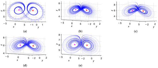
Figure 1.
Three-dimensional chaotic attractors of the system for various q values when : (a) , (b) , (c) , (d) , (e) . Red and pink stars represent and , respectively.
3. Dynamic Analysis of Discrete FODM-DE Chaotic System
We investigate the discrete FODM-DE chaotic system (10), obtained via the piecewise constant argument method [33]. Numerical simulations are performed in MATLAB 2022a to explore its dynamical behavior under integer, fractional, and variable fractional orders. Our primary focus is on analyzing the dynamic behavior of the discrete FODM-DE system under varying fractional orders and system parameters. For comparison, we also examine its dynamics in both integer-order and fixed fractional-order cases, with all discretizations performed using the piecewise constant argument method.
To investigate the dynamics of the fractional system (10), we analyze the system by treating the parameter p as the bifurcation parameter and generating bifurcation diagrams to capture its behavior. Specifically, we vary with , using initial conditions (, , ) = (1, 1, 1), and perform simulations over iterations.
To investigate the chaotic dynamics of the proposed discrete-time system, the maximum Lyapunov exponent (MLE) was estimated directly from the scalar time series using the method introduced by Rosenstein et al. [36]. This technique is applicable to both continuous and discrete systems and does not require explicit knowledge of the system equations.
The first step involves reconstructing the state space using the method of time-delay embedding. From the one-dimensional discrete-time series , the embedded vectors are formed as
where is the time delay (in iterations) and m is the embedding dimension.
For each vector , its nearest neighbor is found such that to avoid temporally correlated points. The divergence between initially close states is tracked over time steps:
In a chaotic system, nearby trajectories diverge exponentially, and thus, the average log-distance increases linearly with :
Here, is the estimated maximum Lyapunov exponent, and K is a constant. The exponent is calculated as the slope of the linear portion of the log-divergence curve.
As commonly understood, a system exhibits chaotic behavior when its maximum Lyapunov exponent, MLE, is positive. This positivity indicates a high sensitivity to initial conditions and the presence of complex, unpredictable dynamics.
3.1. Integer-Order Case
In the integer-order case, the order parameter was set to , effectively reducing the system (10) to its classical (non-fractional) counterpart. To explore the nonlinear behavior of the system in this case, a bifurcation analysis was carried out by treating the system parameter p as the bifurcation parameter, varied within the range . Using the PWCAD, the system was simulated over 50,000 iterations with initial conditions . The resulting bifurcation diagram, shown in Figure 2, reveals a rich sequence of dynamic transitions as p decreases from fixed-point stability to periodic oscillations and ultimately to chaotic regimes. The diagram clearly illustrates the onset of chaos beyond a certain threshold of p, characterized by a dense scattering of points and the absence of periodic windows.
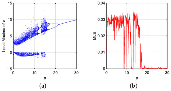
Figure 2.
Dynamic analysis of the discrete DM-DE system for parameter p when : (a) bifurcation diagram, (b) MLE.
To validate and quantify the chaotic behavior observed in the bifurcation diagram, MLE was computed over the same range of p values. The computed MLE for each value of p is also presented in Figure 2. The results confirm that the system exhibits chaotic behavior for regions where MLE > 0, corresponding to intervals in p where the bifurcation diagram indicates high sensitivity and complex oscillatory patterns. Conversely, for larger values of p, the Lyapunov exponent remains near zero, indicating that the system trajectories converge to fixed points or limit cycles.
3.2. Fractional-Order Case
To examine the influence of fractional-order dynamics on the system behavior, the q was varied in the interval while keeping the system parameter fixed at . This range allows exploration of how memory effects and non-local interactions introduced by fractional calculus alter the stability and complexity of the discrete FODM-DE system. The bifurcation diagram in Figure 3 reveals that as q decreases from 1 to 0.6, the system undergoes qualitative changes in its dynamical behavior. The emergence of periodic windows, intermittent chaotic bursts, and dense bifurcation branches indicates enhanced sensitivity to fractional-order variation.
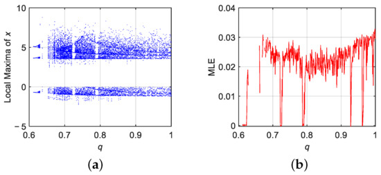
Figure 3.
Dynamic analysis of the discrete FODM-DE system for when : (a) bifurcation diagram, (b) MLE.
To validate the observed dynamics quantitatively, MLE was computed across the same range of q values. As illustrated in Figure 3, the Lyapunov exponent curve confirms the presence of chaotic behavior for a broad subset of the fractional-order domain, where MLE > 0. Interestingly, in previous studies on the same system [29,37], chaos was not observed below the commensurate-order threshold of . In contrast, by employing the PWCAD method in this work, chaotic flows are obtained even for q values as low as 0.6. This clearly demonstrates that the adopted discretization approach enhances the system’s complexity and broadens its chaotic range without altering the classical system parameters. Overall, the results affirm that the piecewise constant argument method provides a more powerful framework for capturing richer and more flexible dynamical regimes compared to those reported using conventional approaches.
3.3. Commensurate Variable Fractional-Order Case
Transforming the previously defined fractional-order derivative operator q into its fractional variable-order counterpart yields a refined formulation of the discrete FVODM-DE chaotic system.
where . The primary objective is to investigate the dynamic behavior of the FVODM-DE system (16), influenced by both the fractional variable order and the system parameter p. To illustrate the system’s dynamics, we considered the case where with initial conditions . We examined four distinct profiles of the fractional-order function as , , , and . The sinusoidal profile models slow periodic modulation of memory, while the exponential-based profile represents smooth but non-periodic evolution. In contrast, the signum-based profile produces abrupt switching between two order levels, and the high-frequency signum profile induces rapid switching dynamics. These complementary profiles allow investigating of the system’s robustness and sensitivity under gradual, smooth, and abrupt variations in fractional order, providing insights into the role of memory variability in chaotic dynamics.
Figure 4 presents a comprehensive dynamic analysis of the FVODM-DE system using bifurcation diagrams (Figure 4a–d) and the corresponding maximum Lyapunov exponent (MLE) spectra (Figure 4e–h) for each variable-order function , , , and . The bifurcation diagrams demonstrate how the local maxima of the state variable x evolve as the system parameter p varies from 0 to 15. Each diagram reveals rich dynamical behaviors, including periodic windows, chaotic regimes, and sudden transitions, depending on the shape and characteristics of the chosen fractional-order profile. In particular, the sinusoidal and exponential variations in induce smoother transitions, while the signum-based profiles generate more abrupt bifurcation structures, highlighting the sensitivity of the system’s dynamics to the structure of the fractional-order function.
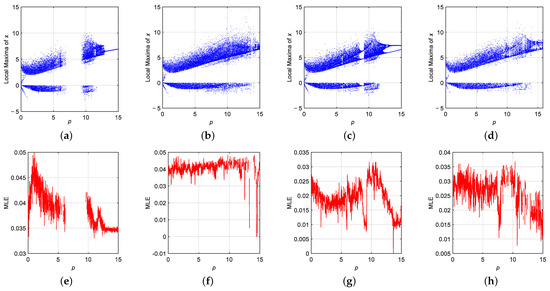
Figure 4.
Dynamic analysis of the VFODM-DE system for p: (a–d) bifurcation diagrams for , and ; (e–h) MLEs for , and , respectively.
The MLE plots provide further insight into the chaotic characteristics of the system by quantifying the divergence rate of nearby trajectories. Positive Lyapunov exponents across wide parameter ranges confirm the existence of chaos in the system, especially for and , where sustained high values of MLE indicate robust chaotic behavior. On the other hand, and profiles exhibit intermittent periodicity, evidenced by the occasional dips of the MLE towards zero. These results confirm that the dynamic response of the FVODM-DE system is highly tunable through both the parametric variation and the design of the VFO function.
3.4. Symmetry Analysis of the VFODM-DE System
A transformation is called a symmetry of the system if the system’s dynamics commute with S, i.e., , where F denotes the right-hand side vector field defining the system dynamics. Meanwhile, the fixed points of system (16) appear as , which suggests that the mapping may represent a system symmetry. To verify this, define the nonlinear components of the system as
Applying the transformation S yields
Therefore, the first two components change sign, while the third remains invariant under S. Consider the discrete-time update equations for the state vector :
where . Applying the transformation S to the updated state, we have
where ⊕ denotes concatenation with the unchanged z-component. On the other hand, evolving the transformed previous state by the system yields
which simplifies to the same expression for . Hence, the system dynamics commute with S, confirming it as a symmetry. This symmetry implies that for any trajectory starting from an initial condition , there exists a symmetric trajectory originating from , whose evolution is the image of the original trajectory under the transformation S.
Figure 5 illustrates the numerical verification of the identified symmetry transformation when and VFO . The blue curves correspond to the trajectory initialized at , while the red curves correspond to the symmetric initial condition . The time series of and reveal that the two signals are sign-inverted counterparts, whereas the component remains identical, in agreement with the analytical results in this section. The three-dimensional phase portrait further confirms that the two trajectories are exact reflections of each other with respect to the -plane. This serves as strong numerical evidence supporting the existence of the symmetry discussed above.
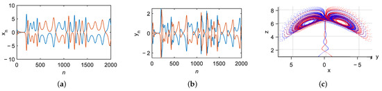
Figure 5.
Two trajectories with symmetric initial conditions, with in blue and in red: time series of (a) , (b) , (c) phase portrait of .
3.5. Multistability with Coexisting Attractors
Multistability is an important nonlinear phenomenon that has attracted considerable attention in the study of chaotic systems. To demonstrate the multistable behavior of the VFODM-DE system, bifurcation diagrams were generated under different fractional-order conditions. For instance, when varying , and varying , as given in Figure 6, distinct dynamical behaviors emerge depending on the choice of initial conditions. Specifically, two sets of initial states were considered: for the blue trajectory and for the red trajectory. The bifurcation diagrams reveal bistability within these parameter ranges, indicating that the system evolves towards different attractors depending on the initial condition.
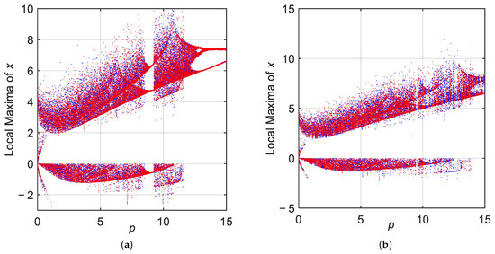
Figure 6.
Bifurcation diagrams for p with two sets of initial conditions: for blue plot and for red plot when (a) , (b) .
To further illustrate this behavior, Figure 7 presents three coexisting attractors obtained under the same system parameters but with different initial states: for the blue trajectory, for the red trajectory, and when varying , and varying . For VFO, the system exhibits multiple coexisting attractors when three or more distinct initial conditions are selected, as shown in Figure 7. This indicates the existence of a complex basin structure with multiple attraction domains.
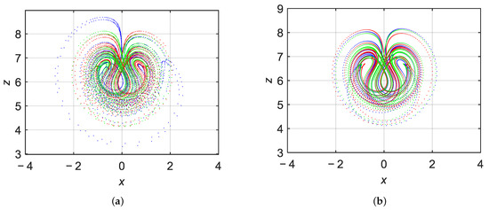
Figure 7.
Coexisting three attractors for with three sets of initial conditions: for blue plot, for red plot, and for green plot when (a) , (b) .
These findings highlight that the VFODM-DE system is not only capable of producing chaotic flows but also exhibits advanced nonlinear phenomena such as multistability, attractor coexistence, and symmetry-related behaviors.
3.6. Hidden Dynamics in the VFODM-DE System
The investigation of system (16) reveals the existence of complex dynamics, including chaotic attractors that are not connected to the local neighborhoods of its equilibrium points. These attractors satisfy the conditions of hidden attractors, as defined in [18,29]. For the parameter set and VFO , the system admits two symmetric equilibria . Linearizing the system around these points and applying Jury stability criterion, it is confirmed that these equilibria are asymptotically stable for all , as detailed in Section Local Stability Analysis via Jury Test.
Despite the presence of stable equilibria, simulations reveal the existence of a chaotic attractor arising from specific initial conditions. For example, when and , the trajectory diverges from the equilibria and converges to a complex, non-periodic orbit characterized by positive Lyapunov exponents. The MLE given in Figure 4 confirms the chaotic nature of this attractor. In a particular scenario, the system exhibits hidden attractors: these are periodic or chaotic attractors that either lack any equilibrium points or coexist only with stable equilibria. A defining feature of such attractors is that their basin of attraction is not connected with the neighborhood of any unstable equilibrium points of the system [18]. Through our investigation, we observed the presence of hidden attractors in this system. Specifically, under the parameter configuration with VFO , the system was found to possess two stable equilibrium points. However, initiating the system from the state leads to the emergence of hidden attractors, as illustrated in Figure 8. Notably, such hidden attractors are absent in the integer-order system, highlighting the greater complexity and richness of the dynamics in VFO chaotic systems.
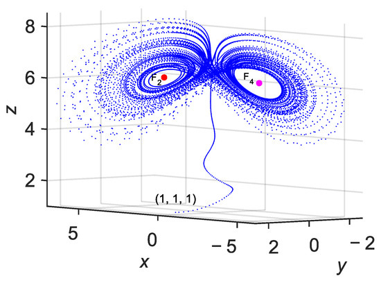
Figure 8.
Hidden attractor when and with .
4. Image Encryption
The developed encryption approach employs a statistically verified VFODM-DE chaotic system-based random number generator to enhance cryptographic strength. Chaotic systems are widely recognized for their sensitivity to initial conditions, ergodicity, and pseudorandom behavior, making them suitable for secure image encryption [26]. However, fixed-order chaotic systems may suffer from limited randomness sources. In contrast, VFO dynamics enrich the entropy pool by introducing temporal variability and hidden attractors, thereby generating more unpredictable keystreams. Such properties are crucial in image encryption, where natural images exhibit high pixel correlation and non-uniform histograms that must be effectively concealed. To this end, the proposed VFODM-DE-based PRNG utilizes both state variables and fractional-order parameters as entropy sources, ensuring statistically robust random bitstreams. The resulting keystreams were comprehensively validated using the NIST SP 800-22 test suite, confirming their suitability for cryptographic applications. The VFODM-DE-based encryption–decryption framework comprises several well-defined stages (see Figure 9), each of which is systematically detailed in the subsequent discussion. For clarity, in the remainder of this section, we use the terms original image, encrypted image, and decrypted image to refer to the plaintext, ciphertext (cipher-image), and recovered image, respectively. This ensures consistency between the cryptographic formulation and the visual demonstrations.
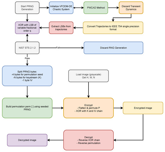
Figure 9.
VFODM-DE-based encryption–decryption process.
4.1. Pseudorandom Number Generator Design Based on VFODM-DE Chaotic System
In this study, a PRNG architecture is proposed by exploiting the high sensitivity and unpredictability of the VFODM-DE chaotic system. The design exploits the system’s three state variables and the fractional-order parameter as entropy sources, in a manner similar to the method presented in [38]. At each discrete iteration, the states , , and are converted to IEEE 754 [39] 32-bit floating-point format and the least-significant byte (LSB, bits 0–7) of each is extracted. The LSB bytes of x, y, and z are XORed to form an intermediate byte. In parallel, the fractional-order parameter is converted to IEEE 754 and its LSB byte is extracted and XORed with the intermediate byte. The resulting bytes are concatenated over iterations to form the final output bitstream.
For the PRNG design, the hidden attractor described in Section 3.6 was utilized where and VFO . The workflow is shown in Algorithm 1. The generated bitstream was evaluated using the NIST SP 800-22 randomness test suite. Representative test results are presented in Table 2. Tests are considered passed when the p-value is greater than the chosen significance level, which is commonly .
Table 2.
Representative NIST SP 800-22 test results.
The design and implementation of the VFODM-DE-based PRNG given in Algorithm 1 can be described as a sequence of well-defined steps, as detailed below:
- Step 1:
- Initialization of System Parameters: The nonlinear chaotic system parameters are first defined, including the control parameter , the integration step size , the total number of iterations , and the initial conditions . In addition, the variable fractional-order sequence is modulated using a signum-based periodic function to induce switching behavior in the system’s memory.
- Step 2:
- Generation of Chaotic Time Series: The state variables , , and are iteratively updated for using the PWCAD method adapted for variable fractional order. Each update involves the computation of the Gamma function and the fractional-order step size , which are used to integrate the system equations and generate the chaotic trajectories.
- Step 3:
- Visualization: After discarding the transient portion of the time series, the three-dimensional chaotic attractor is plotted to verify that the system exhibits the expected chaotic behavior.
- Step 4:
- IEEE 754 Conversion: For each sample n, the values of , , , and are converted into their IEEE 754 single-precision (32-bit) representations. This step ensures a uniform binary representation of the chaotic states, which facilitates subsequent bit-level operations.
- Step 5:
- Extraction of Least Significant Bytes: From each 32-bit floating-point representation, the least significant byte (LSB) is extracted. This approach improves randomness by emphasizing the fine-grained chaotic fluctuations, which are highly sensitive to the system’s initial conditions and parameter variations.
- Step 6:
- XOR-based Mixing: The extracted LSBs of x, y, and z are combined using bitwise XOR operations to produce an intermediate byte. This result is then XORed with the LSB of q to yield the final random byte. This step enhances the statistical uniformity and unpredictability of the output by mixing information from all four chaotic state variables.
- Step 7:
- Bitstream Assembly: Each resulting byte is converted into its 8-bit binary representation, and the bits are concatenated to form a continuous bitstream. This process is repeated for all N samples, producing a sufficiently long binary sequence suitable for statistical testing.
- Step 8:
- Validation and Output: The total number of generated bits is checked to ensure that it satisfies the minimum requirement of at least 1 Mbit, as recommended by the NIST SP800-22 test suite. The final bitstream is then written to a text file (e.g., trng_bits.txt), making it available for use in subsequent encryption and decryption experiments.
| Algorithm 1 Proposed PRNG bit generation from VFODM-DE chaotic system. |
| Require: Chaotic state sequences , , and fractional-order parameter of length N Ensure: Output bitstream B of at least 1 Mbit
|
4.2. Encryption–Decryption Processes
The proposed PRNG-based grayscale image encryption algorithm (Algorithm 2) was applied to six test images of different resolutions to evaluate its performance and robustness: Baby ( pixels), Airplane ( pixels), Couple ( pixels), Aerial ( pixels), Airport ( pixels), and Male ( pixels). The test images were obtained from the USC School of Engineering website (https://sipi.usc.edu/database/database.php) accessed on 1 August 2025. We evaluated the security and efficiency of the proposed encryption algorithm using a computer running MATLAB R2022a. The system was equipped with an Intel i9-13900H, 2.60 GHz processor, and 32 GB of memory. For each image, the generated keystream was used as detailed in Section 4.1. The stored sequence in the text file (prng_bits.txt) is parsed into an unsigned byte array T, from which three components are taken sequentially: a permutation seed (), a keystream byte array (K) with one byte per pixel, and an initial diffusion value () serving as an initialization vector.
Encryption is performed in two consecutive stages. First, the image is flattened into a one-dimensional vector Q of length (row-major order) and permuted according to a Fisher–Yates shuffle seeded with , yielding a permuted vector . This permutation step effectively destroys the spatial correlation between adjacent pixels. Second, a diffusion operation is applied in which each pixel of is XORed with the corresponding keystream byte and then XORed with the previous cipher-pixel (with ) according to
where ⊕ denotes the bitwise XOR. This chaining mechanism ensures that a small change in the plaintext propagates to all subsequent cipher-pixels. The resulting cipher vector C is reshaped into an matrix to produce the cipher-image.
Decryption follows the exact inverse of these steps, using the same values as in encryption. First, inverse diffusion is applied:
recovering the permuted plaintext pixels. Then, the inverse permutation is applied to to restore the original pixel order, yielding the decrypted image . Reshaping back to yields a reconstruction identical to the original image I, confirming correct decryption.
The entire VFODM-DE-based encryption–decryption framework given in Figure 9 consists of a series of structured steps, which are described below.
- Step 1:
- Reading and Preprocessing the PRNG Output: The bitstream generated by the VFODM-DE-based random number generator (stored in prng_bits.txt) is read as a sequence of characters composed of ‘0’ and ‘1’. All non-binary characters are removed, and if the total number of bits is not a multiple of 8, zero-padding is applied to reach the nearest byte boundary. This ensures that the bitstream can be grouped into complete bytes for subsequent operations.
- Step 2:
- Conversion of Bits to Bytes: The cleaned binary stream is grouped into 8-bit segments, and each group is converted to its corresponding decimal value to obtain an array of 8-bit unsigned integers (uint8). This operation transforms the raw TRNG output into a form suitable for use as cryptographic keystream and permutation seeds.
- Step 3:
- Image Loading and Preparation: The selected plaintext image (e.g., Airport.tiff) is loaded. The image is then cast to uint8 format, and its height (H), width (W), and total number of pixels () are computed. These parameters determine how many bytes from the TRNG output are needed for the encryption process.
- Step 4:
- Keystream Segmentation and Parameter Extraction: The PRNG byte sequence is divided into three parts: (i) the first 4 bytes are used as a seed for generating a random pixel permutation, (ii) the next N bytes serve as the encryption keystream (K), and (iii) one additional byte is reserved as an initialization vector (IV). This segmentation ensures both confusion (through permutation) and diffusion (through keystream masking).
- Step 5:
- Generation of Pixel Permutation: A 4-byte segment denoted as is extracted from the initial part of the PRNG byte stream and typecast into a 32-bit integer seed. This seed is then used to initialize the pseudorandom number generator. Based on this seeded RNG, a pseudorandom permutation over the index set is constructed using the Fisher–Yates shuffling algorithm. This permutation determines the new positions of the N pixels in the flattened image vector, thereby providing confusion at the pixel level prior to the diffusion process.
- Step 6:
- Encryption Process: The plaintext image is first flattened into a one-dimensional pixel vector and then permuted according to the previously generated permutation . After permutation, each pixel is encrypted using the keystream K through a chained XOR-based diffusion process, where the output of each step depends on both the current pixel and the previous ciphertext byte (initialized by the IV). Finally, the resulting encrypted bytes are reshaped back to the original image dimensions to obtain the ciphertext image.
- Step 7:
- Decryption Process: Decryption uses the same permutation , keystream K, and IV values as in the encryption stage. Each ciphertext byte is processed through the inverse of the diffusion operation to recover the permuted plaintext sequence, after which the inverse permutation is applied to restore the original pixel order. The recovered pixels are then reshaped into their original two-dimensional format to reconstruct the plaintext image.
- Step 8:
- Correctness Verification: Finally, the decrypted image is compared to the original plaintext image on a pixel-by-pixel basis using the isequal function. If the encryption and decryption procedures are implemented correctly, the two images are identical, confirming lossless recovery of the original data.
This process was executed independently for each test image to avoid keystream reuse, thereby enhancing security. Visual inspection of the cipher-images, as shown in Figure 10, reveals completely noise-like patterns without any recognizable structures from the original images. The subsequent subsections provide quantitative analyses, including histogram uniformity, correlation coefficient reduction, and entropy evaluation, to further validate the security of the proposed scheme.
| Algorithm 2 PRNG-based grayscale image encryption. |
| Require: Grayscale image I of size , PRNG bitstream file prng_bits.txt Ensure: Cipher image C
|
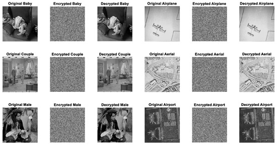
Figure 10.
Original, encrypted, and decrypted images.
4.3. Security and Efficiency Evaluations
To confirm the cryptographic strength of the proposed encryption algorithm, a series of security analyses were performed against various known attacks. This subsection details the evaluation of the algorithm based on several standard security metrics.
4.3.1. Key Space Analysis
Key space refers to the total number of possible distinct secret keys that can be generated by an encryption system. A sufficiently large key space is essential to resist brute-force attacks, as an attacker would have to try all possible keys to decrypt the ciphertext without authorization. For modern image encryption applications, the minimum acceptable key space is generally considered to be [40]. In the proposed scheme, the secret key is generated from the initial conditions and system parameters of the VFODM–DE chaotic system. Specifically, the secret key comprises four components, which are with double-precision floating-point numbers, each having approximately resolution. Each state contributes about 15 decimal digits of precision, which corresponds to roughly possibilities. Therefore, the total number of possible key combinations can be estimated as
This extremely large key space ensures that the proposed encryption scheme is effectively immune to exhaustive brute-force attacks, thereby guaranteeing the security of encrypted images against unauthorized decryption attempts.
4.3.2. Key Sensitivity Analysis
Key sensitivity is a fundamental security property of chaos-based encryption systems. It ensures that even an extremely small change in any secret key parameter leads to a completely different encryption result. This property makes brute-force attacks impractical, because an attacker cannot obtain any useful information unless the exact secret key is used.
To evaluate the key sensitivity of the proposed VFODM–DE-based image encryption scheme, we performed a set of experiments using the standard Airport image. The image was encrypted using the original key. Then, the encryption was modified slightly by altering a single key element by only (). The visual results are shown in Figure 11, which presents (a) the original Airplane image, (b) the encrypted image with the correct key, (c) the encrypted image obtained with , and (d) the absolute difference images between (b) and (c).
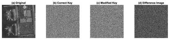
Figure 11.
Key sensitivity experimental results: (a) original image, (b) encrypted image obtained by (b) correct key, (c) modified key, (d) difference of (b,c).
It can be clearly observed that modified key produces a completely different encrypted image. Furthermore, the difference images appear noise-like, confirming that there is no visual similarity between encrypted images. These results demonstrate that the proposed scheme has excellent key sensitivity, which ensures that only the exact secret key can correctly decrypt the ciphertext, thereby significantly enhancing the security of the system.
4.3.3. Histogram Uniformity Analysis
A secure image encryption scheme should produce cipher-images whose gray-level histograms are uniformly distributed. In a well-encrypted image, each intensity value in the range should occur with approximately equal probability, making statistical attacks based on frequency analysis ineffective.
For each of the three test images, histograms of the original, encrypted, and decrypted versions were computed and compared. As shown in Figure 12, the plaintext images exhibit highly non-uniform histograms with characteristic peaks and valleys related to their semantic content, whereas the cipher-images show almost ideally flat histograms, indicating a uniform distribution of pixel values. This uniformity confirms that the proposed encryption scheme effectively conceals the statistical structure of the original images, thereby enhancing resistance against histogram-based cryptanalysis.
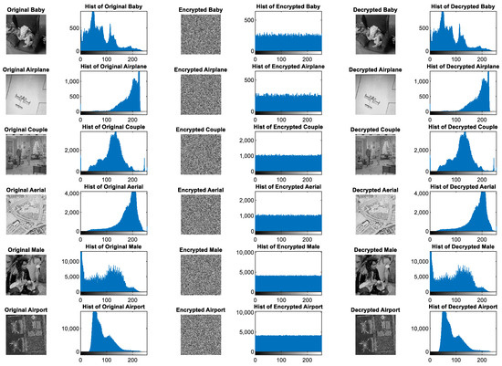
Figure 12.
Original, encrypted, and decrypted images with their corresponding histograms.
Moreover, the decrypted images show histograms that closely match those of the original counterparts. This consistency demonstrates that the encryption–decryption process not only provides strong security through histogram uniformity of the cipher-images, but also guarantees lossless recovery of the plaintext images.
4.3.4. Correlation Coefficient Reduction
In natural images, adjacent pixels are highly correlated, especially in smooth regions. An effective encryption scheme must reduce this correlation to a value close to zero. The correlation coefficient between two adjacent pixels is computed using [41]
where is the covariance, and and are the standard deviations of the gray levels of adjacent pixels x and y.
For each test image, correlation coefficients were measured in horizontal, vertical, and diagonal directions for both plaintext and cipher-images. As reported in Table 3, the plaintext images exhibit high correlation values (>0.90), whereas the cipher-images display values very close to zero, some even slightly negative similar to those obtained in Lena, biomedical, and other benchmark images reported in [26,42,43]. This significant reduction demonstrates that the proposed method effectively removes pixel-to-pixel dependencies, thereby thwarting attacks exploiting spatial redundancy.
Table 3.
Correlation coefficients of original and encrypted images.
4.3.5. Information Entropy Evaluation
Information entropy measures the unpredictability of information content in an image. For an ideal cipher-image using 8-bit gray levels, the entropy should be close to the maximum value of 8 bits. The entropy for a discrete source is calculated as [47]
where is the probability of occurrence of the gray level .
The entropies of the plaintext images are significantly lower than 8, reflecting the redundancy in natural image data. In contrast, the encrypted images exhibit entropy values very close to 8 as summarized in Table 4, consistent with the nearly optimal entropies reported for Lena and biomedical images in [42,43]. This indicates that the VFODM-DE chaotic system achieves state-of-the-art randomness comparable to other recent chaotic encryption frameworks. It is confirmed that the cipher-images leak minimal information about the original images, thereby providing strong resistance against entropy-based statistical attacks.
Table 4.
Information entropy of original and encrypted images.
4.3.6. Differential Attack Analysis Using NPCR and UACI
To evaluate the sensitivity of the proposed encryption algorithm against differential attacks, two standard metrics, NPCR and UACI, are computed [48]. These metrics quantify how significantly the encrypted image changes in response to a small modification in the original image.
The NPCR and UACI values for three test images are summarized in Table 5. The results are highly consistent with benchmark values (around 99.6% and 33%, respectively) reported in [26,42,43], confirming that the proposed scheme provides robustness against differential attacks at the same level as other state-of-the-art encryption algorithms. As observed from Table 5, all NPCR values are very close to 100%, and UACI values are around 33%, indicating that the encryption algorithm is highly sensitive to small changes in the plaintext images. This demonstrates strong resistance to differential attacks, ensuring the robustness of the proposed encryption scheme.
Table 5.
NPCR and UACI values for differential attack analysis.
4.3.7. Robustness Analysis
The robustness of an image encryption algorithm against data loss is a critical security measure for applications in unstable communication channels where data corruption can occur. A robust encryption scheme must possess strong diffusion, ensuring that even minor data loss in the encrypted image results in significant, widespread distortion in the decrypted image, thereby preserving the security of the original image. To evaluate the robustness of our proposed encryption scheme, a series of data loss simulations were conducted by applying intentional corruption to the encrypted image.
Instead of distributing the damage randomly across the entire image, we applied a defined loss to five distinct, randomly chosen rectangular regions of the encrypted image. This method provides a focused examination of the algorithm’s diffusion properties. In each of the four trials, a 40% × 40% rectangular area was subjected to a complete data loss, simulating a severe and localized corruption. The damaged encrypted images were then decrypted to observe the resulting impact on the original image’s content.
As illustrated in Figure 13, the simulation results provide compelling evidence of the encryption scheme’s resilience. The top row of the figure displays the encrypted images with the applied localized damage, represented by black squares in different random locations. The bottom row shows the corresponding decrypted images. Although the damage was confined to small regions in the encrypted image, the decryption process caused the effect of this data loss to propagate throughout the entire image.
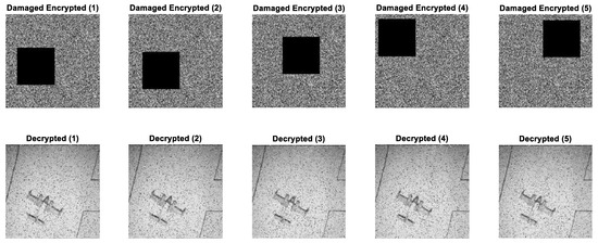
Figure 13.
Robustness analysis results.
The visual output shows a heavily distorted image of the airplane, with its background and form corrupted by a significant number of randomly scattered pixels. This widespread distortion is a direct result of the strong diffusion properties of the encryption algorithm, which effectively scatter the effects of a single damaged pixel across the entire image during the decryption process. This outcome validates the algorithm’s capability to withstand data loss and reinforces its suitability for secure multimedia transmission.
4.3.8. Encryption Efficiency Evaluation
The efficiency of an encryption algorithm is a critical metric for its practical application, especially in time-sensitive scenarios. A high-performing algorithm must be computationally efficient to be viable for real-time systems. In this study, we conducted a systematic evaluation of our proposed encryption scheme’s efficiency to demonstrate its suitability for demanding applications.
The efficiency of an encryption algorithm is typically quantified by its throughput, which measures the amount of data processed per unit of time. This metric is calculated by dividing the total data size of an image in bits by the total time elapsed during the encryption or decryption process in seconds. We measured the encryption and decryption performance on grayscale images of sizes 256 × 256, 512 × 512, and 1024 × 1024, and the results highlight the high-speed capability of our algorithm across different scales. For the 256 × 256 image, the encryption efficiency was 325.48 Mbps, while the decryption efficiency was 347.51 Mbps. For the 512 × 512 image, these values were 487.88 Mbps and 538.26 Mbps, respectively. Finally, for the 1024 × 1024 image, our algorithm achieved an encryption efficiency of 647.56 Mbps and a decryption efficiency of 628.85 Mbps.
When compared with existing schemes, as shown in Table 6, our algorithm demonstrates competitive performance, achieving high throughput speeds that are essential for real-time applications. These results indicate that the proposed algorithm delivers exceptional performance, with throughput scaling effectively as image size increases. This combination of high efficiency and robust security features positions our scheme as a highly practical and competitive solution for secure image transmission in various applications, including those requiring real-time processing.
Table 6.
Average encryption times in second achieved by proposed method and recent schemes.
5. Results and Discussion
The VFODM-DE chaotic system was comprehensively evaluated through both dynamical analysis and cryptographic performance assessments. The discrete fractional-order DM–DE chaotic system under consideration is governed by Equation (10), where denotes the step size, is the control parameter, and represents the VFO. Unless otherwise specified, the system is initialized at . To explore the dynamical behavior, several distinct functional forms of were considered. The bifurcation diagrams and corresponding Lyapunov exponent spectra shown in Figure 4 confirm that chaos emerges at significantly lower fractional orders compared to conventional fractional-order analyses in the literature reported in [29,37].
The system also displays hidden dynamics under specific parameter conditions. For instance, when and , a hidden attractor emerges coexisting with stable equilibria, as illustrated in Figure 8. In addition, symmetry tests revealed that trajectories initialized at and evolve as mirrored counterparts in the plane (Figure 5), demonstrating structural invariance. Similarly, Figure 7 shows that distinct attractors coexist for identical parameters but different initial states, evidencing multistability. These results highlight that the memory effect introduced by enriches the system Jacobian, thereby enabling the coexistence of multiple dynamical regimes in the same parameter space.
The chaotic sequences obtained from the VFODM-DE system were then utilized to construct a PRNG. The statistical validation through the NIST SP 800-22 test suite (Table 2) confirmed that the generated bitstreams pass all randomness tests, ensuring their suitability for cryptographic use. Leveraging these outputs, the proposed image encryption framework was applied to test images (Baby, Airplane, Couple, Aerial, Male, Airport), producing cipher-images with noise-like appearance (Figure 10). The key space of the proposed scheme, generated from the initial conditions and system parameters of the VFODM-DE system (), is extremely large, approximately , far exceeding the typical minimum requirement of . This ensures that the system is practically immune to brute-force attacks. In addition, the encryption demonstrates very high key sensitivity: even a minuscule change in a single key parameter, e.g., variation in , results in a completely different encrypted image, as shown in Figure 11. The difference images are noise-like, indicating no correlation with the ciphertext generated using the original key, and thus, only the exact key can successfully decrypt the ciphertext. Histogram analysis (Figure 12) revealed that the encrypted images exhibit nearly uniform gray-level distributions, effectively concealing statistical structures of the plaintext. Correlation coefficients between adjacent pixels (Table 3) dropped from values exceeding in plaintexts to values close to zero or slightly negative in ciphertexts. Information entropy results (Table 4) further demonstrated near-ideal values close to 8, consistent with optimal randomness. Finally, NPCR and UACI metrics (Table 5) confirmed strong resistance against differential attacks, with results around and , respectively. Comparison with benchmark studies [26,42,43,44,46,46] demonstrates that VFODM-DE-based encryption framework achieves equivalent or superior performance across all metrics. Encryption efficiency was also evaluated to assess practical applicability. The throughput of the proposed method scales well with image size: 325.48/347.51 Mbps for 256 × 256, 487.88/538.26 Mbps for 512 × 512, and 647.56/628.85 Mbps for 1024 × 1024 grayscale images (encryption/decryption). Compared to recent schemes [21,26,49,50], the proposed algorithm achieves higher throughput and faster computation times (Table 6), confirming its suitability for real-time secure image transmission.
In terms of practical relevance, the proposed VFODM-DE-based encryption framework offers a promising solution for secure multimedia data protection in real-time environments, where both high security and computational efficiency are critical. The high throughput achieved by the scheme makes it suitable for real-time secure image transmission in applications such as telemedicine, surveillance systems, and Internet of Things (IoT) devices operating with limited computational resources. Furthermore, the strong key sensitivity and large key space provide resilience against brute-force and statistical attacks, ensuring robustness in practical deployments. However, the current implementation has certain limitations: the experiments were conducted on grayscale images and in a software-based environment without hardware optimization. Moreover, the PWCAD method has certain limitations. Since it approximates the system dynamics using piecewise constant steps, the method can introduce approximation errors and phase distortions, especially when larger step sizes are used. It may also smooth out fast-changing dynamics, potentially obscuring high-frequency behaviors of the system. Moreover, due to the memory-dependent nature of fractional-order systems, small numerical errors in PWCAD-based simulations may accumulate over time, affecting long-term accuracy. Additionally, the method is primarily suited for Caputo-type derivatives and requires significant adaptation for other fractional derivative definitions, which can limit its general applicability.
Overall, integrating these results shows that the VFODM-DE system not only exhibits rich nonlinear behavior, including multistability and hidden attractors, but also provides a reliable foundation for cryptographic applications. The memory effect induced by significantly enhances the system’s unpredictability, which improves the PRNG output quality. Combined with a large key space, excellent key sensitivity, and high encryption efficiency, the proposed VFODM-DE-based image encryption framework presents a highly secure and practical solution for modern image protection, outperforming or matching benchmark methods across all considered metrics.
6. Conclusions
This study was motivated by the limitations of existing fractional-order chaotic systems used in image encryption, which are mostly based on fixed-order dynamics and conventional numerical solvers. Such approaches often reduce chaotic complexity, limit key diversity, and overlook hidden dynamics, thereby restricting their security potential. To overcome these shortcomings, we proposed a discrete VFODM-DE chaotic system discretized using the PWCAD method. This approach enables chaos to emerge at significantly lower fractional orders while reducing computational burden, which is crucial for long-term simulations and practical implementations. Through comprehensive analyses, we demonstrated several distinctive dynamical properties of the proposed system, including multistability, symmetry, coexisting attractors, and hidden dynamics despite the presence of stable equilibria. These findings reveal richer nonlinear behaviors than those observed in fixed-order models, highlighting the enhanced complexity introduced by variable fractional-order dynamics. Leveraging these properties, we constructed a PRNG and developed a lightweight image encryption scheme. Extensive security evaluations showed that the proposed method achieves a large key space (), near-ideal histogram uniformity, extremely low adjacent-pixel correlation (<0.04), high information entropy (>7.999), strong resistance against differential attacks (NPCR ≈ 99.6%, UACI ≈ 33.46%), and high throughput (≈647.56 Mbps), outperforming many existing schemes in both security and efficiency. While the proposed scheme demonstrates strong cryptographic performance, it also has certain limitations. The current implementation has been validated on grayscale images only, and its performance under hardware constraints or real-time streaming conditions has not yet been explored. Furthermore, the effect of different variable-order functions on the long-term statistical properties of the PRNG requires more extensive theoretical analysis. In future work, we aim to extend the proposed VFODM-DE-based framework to color images and video encryption and investigate its hardware implementations using FPGA or embedded platforms for real-time applications. Overall, this study shows that combining variable fractional-order dynamics with PWCAD offers a powerful paradigm for constructing highly secure and efficient chaos-based encryption systems.
Funding
This research was funded by Scientific Research Project Fund of Balikesir University under the project number BAP 2025/169.
Data Availability Statement
The original contributions presented in the study are included in the article. Further inquiries can be directed to the corresponding author.
Conflicts of Interest
The authors declare no conflicts of interest.
Abbreviations
The following abbreviations are used in this manuscript:
| FODM-DE | Fractional-order dark matter–dark energy |
| PWCAD | Piecewise constant argument discretization |
| VFO | Variable fractional order |
| PRNG | Pseudorandom number generator |
| MLE | Maximum Lyapunov exponent |
| LSB | Least significant byte |
| NPCR | Number of pixels change rate |
| UACI | Unified average changing intensity |
References
- Iqbal, S.; Wang, J. Analysis of a Novel Fractional order Hyper-chaotic System: Dynamics, Stability and Synchronization analysis. Phys. Lett. A 2025, 130770. [Google Scholar] [CrossRef]
- Gökyıldırım, A. Dynamical Analysis and Electronic Circuit Implementation of Fractional-order Chen System. Chaos Theory Appl. 2023, 5, 127–132. [Google Scholar] [CrossRef]
- Demirtas, M.; Ahmad, F. Fractional fuzzy PI controller using particle swarm optimization to improve power factor by boost converter. Int. J. Optim. Control. Theor. Appl. (IJOCTA) 2023, 13, 205–213. [Google Scholar] [CrossRef]
- Lenka, B.K.; Upadhyay, R.K. Synchronization in master–slave ψ-Caputo fractional systems. Nonlinear Dyn. 2025, 113, 19987–20000. [Google Scholar] [CrossRef]
- Hu, H.; Cao, Y.; Hao, J.; Li, X.; Mou, J. A novel chaotic system with hidden attractor and its application in color image encryption. Multimed. Tools Appl. 2023, 82, 4343–4369. [Google Scholar] [CrossRef]
- Diethelm, K.; Ford, N.J.; Freed, A.D. A predictor-corrector approach for the numerical solution of fractional differential equations. Nonlinear Dyn. 2002, 29, 3–22. [Google Scholar] [CrossRef]
- Li, H.; Shen, Y.; Han, Y.; Dong, J.; Li, J. Determining Lyapunov exponents of fractional-order systems: A general method based on memory principle. Chaos Solitons Fractals 2023, 168, 113167. [Google Scholar] [CrossRef]
- Kartal, S.; Gurcan, F. Discretization of conformable fractional differential equations by a piecewise constant approximation. Int. J. Comput. Math. 2019, 96, 1849–1860. [Google Scholar] [CrossRef]
- Tian, H.; Yi, X.; Zhang, Y.; Wang, Z.; Xi, X.; Liu, J. Dynamical Analysis, Feedback Control Circuit Implementation, and Fixed-Time Sliding Mode Synchronization of a Novel 4D Chaotic System. Symmetry 2025, 17, 1252. [Google Scholar] [CrossRef]
- Nabil, H.; Tayeb, H. A secure communication scheme based on generalized modified projective synchronization of a new 4-D fractional-order hyperchaotic system. Phys. Scr. 2024, 99, 095203. [Google Scholar] [CrossRef]
- Akgul, A.; Yaz, M.; Emin, B. Chaos-based approaches to data security: Analysis of incommensurate fractional-order Arneodo chaotic system and engineering application on a microcomputer. Integration 2025, 102, 102355. [Google Scholar] [CrossRef]
- Al-Taani, H.; Abu Hammad, M.; Abudayah, M.; Diabi, L.; Ouannas, A. Asymmetry and symmetry in new three-dimensional chaotic map with commensurate and incommensurate fractional orders. Symmetry 2024, 16, 1447. [Google Scholar] [CrossRef]
- Hammouch, Z.; Yavuz, M.; Özdemir, N. Numerical solutions and synchronization of a variable-order fractional chaotic system. Math. Model. Numer. Simul. Appl. 2021, 1, 11–23. [Google Scholar] [CrossRef]
- Allogmany, R.; Almuallem, N.A.; Alsemiry, R.D.; Abdoon, M.A. Exploring Chaos in Fractional Order Systems: A Study of Constant and Variable-Order Dynamics. Symmetry 2025, 17, 605. [Google Scholar] [CrossRef]
- Wei, Z.; Akgul, A.; Kocamaz, U.E.; Moroz, I.; Zhang, W. Control, electronic circuit application and fractional-order analysis of hidden chaotic attractors in the self-exciting homopolar disc dynamo. Chaos Solitons Fractals 2018, 111, 157–168. [Google Scholar] [CrossRef]
- Matouk, A. Chaotic attractors that exist only in fractional-order case. J. Adv. Res. 2023, 45, 183–192. [Google Scholar] [CrossRef]
- Danca, M.F.; Kuznetsov, N.V.; Chen, G. Approximating hidden chaotic attractors via parameter switching. Chaos 2018, 28, 013127. [Google Scholar] [CrossRef]
- Danca, M.F. Hidden chaotic attractors in fractional-order systems. Nonlinear Dyn. 2017, 89, 577–586. [Google Scholar] [CrossRef]
- Lai, Q.; Yang, L.; Liu, Y. Design and realization of discrete memristive hyperchaotic map with application in image encryption. Chaos Solitons Fractals 2022, 165, 112781. [Google Scholar] [CrossRef]
- Yu, F.; He, S.; Yao, W.; Cai, S.; Xu, Q. Bursting firings in memristive hopfield neural network with image encryption and hardware implementation. IEEE Trans. Comput. Aided Des. Integr. Circuits Syst. 2025. [Google Scholar] [CrossRef]
- Feng, W.; Zhang, K.; Zhang, J.; Zhao, X.; Chen, Y.; Cai, B.; Zhu, Z.; Wen, H.; Ye, C. Integrating Fractional-Order Hopfield Neural Network with Differentiated Encryption: Achieving High-Performance Privacy Protection for Medical Images. Fractal Fract. 2025, 9, 426. [Google Scholar] [CrossRef]
- Liu, Q.; Wang, Y.; Wang, J.; Wang, Q.H. Optical image encryption using chaos-based compressed sensing and phase-shifting interference in fractional wavelet domain. Opt. Rev. 2018, 25, 46–55. [Google Scholar] [CrossRef]
- Roy, M.; Chakraborty, S.; Mali, K. An evolutionary image encryption system with chaos theory and DNA encoding. Multimed. Tools Appl. 2023, 82, 33607–33635. [Google Scholar] [CrossRef]
- Kumari, M.; Gupta, S. Performance comparison between Chaos and quantum-chaos based image encryption techniques. Multimed. Tools Appl. 2021, 80, 33213–33255. [Google Scholar] [CrossRef] [PubMed]
- Li, H.; Yu, S.; Feng, W.; Chen, Y.; Zhang, J.; Qin, Z.; Zhu, Z.; Wozniak, M. Exploiting dynamic vector-level operations and a 2D-enhanced logistic modular map for efficient chaotic image encryption. Entropy 2023, 25, 1147. [Google Scholar] [CrossRef]
- Iqbal, S.; Wang, J.; Calgan, H. Fractional chaotic dynamics in the rucklidge system and its application to image encryption. Nonlinear Dyn. 2025, 1–25. [Google Scholar] [CrossRef]
- Wu, G.C.; Deng, Z.G.; Baleanu, D.; Zeng, D.Q. New variable-order fractional chaotic systems for fast image encryption. Chaos 2019, 29, 083103. [Google Scholar] [CrossRef]
- Aydiner, E. Chaotic Interaction Between Dark Matter and Dark Energy. Int. J. Theor. Phys. 2025, 64, 1–17. [Google Scholar] [CrossRef]
- Danca, M.F. Chaotic hidden attractor in a fractional order system modeling the interaction between dark matter and dark energy. Commun. Nonlinear Sci. Numer. Simul. 2024, 131, 107838. [Google Scholar] [CrossRef]
- Demirtas, M.; Sharkh, S.M.; Gokyildirim, A.; Calgan, H. Secure operation of a stand-alone wind energy system based on an incommensurate fractional-order chaotic system. Appl. Energy 2025, 384, 125477. [Google Scholar] [CrossRef]
- Ucar, E.; Özdemir, N.; Altun, E. Fractional order model of immune cells influenced by cancer cells. Math. Model. Nat. Phenom. 2019, 14, 308. [Google Scholar] [CrossRef]
- El Raheem, Z.; Salman, S. On a discretization process of fractional-order logistic differential equation. J. Egypt. Math. Soc. 2014, 22, 407–412. [Google Scholar] [CrossRef]
- Agarwal, R.P.; El-Sayed, A.M.; Salman, S.M. Fractional-order Chua’s system: Discretization, bifurcation and chaos. Adv. Differ. Equ. 2013, 2013, 1–13. [Google Scholar] [CrossRef]
- Emin, B.; Akgul, A.; Horasan, F.; Gokyildirim, A.; Calgan, H.; Volos, C. Secure encryption of biomedical images based on Arneodo chaotic system with the lowest fractional-order value. Electronics 2024, 13, 2122. [Google Scholar] [CrossRef]
- El-Sayed, A.; Salman, S. On a discretization process of fractional-order Riccati differential equation. J. Fract. Calc. Appl 2013, 4, 251–259. [Google Scholar]
- Rosenstein, M.T.; Collins, J.J.; De Luca, C.J. A practical method for calculating largest Lyapunov exponents from small data sets. Phys. D Nonlinear Phenom. 1993, 65, 117–134. [Google Scholar] [CrossRef]
- Calgan, H. Incommensurate fractional-order analysis of a chaotic system based on interaction between dark matter and dark energy with engineering applications. Phys. A Stat. Mech. Its Appl. 2024, 635, 129490. [Google Scholar] [CrossRef]
- Hosbas, M.Z.; Emin, B.; Kaçar, F. True Random Number Generator Design with A Fractional Order Sprott B Chaotic System. ADBA Comput. Sci. 2025, 2, 50–55. [Google Scholar] [CrossRef]
- IEEE Std 754-2019; IEEE Standard for Floating-Point Arithmetic. IEEE: New York, NY, USA, 2019.
- Feng, W.; Zhang, J.; Chen, Y.; Qin, Z.; Zhang, Y.; Ahmad, M.; Woźniak, M. Exploiting robust quadratic polynomial hyperchaotic map and pixel fusion strategy for efficient image encryption. Expert Syst. Appl. 2024, 246, 123190. [Google Scholar] [CrossRef]
- Sambas, A.; Benkouider, K.; Kaçar, S.; Ceylan, N.; Vaidyanathan, S.; Sulaiman, I.M.; Mohamed, M.A.; Ayob, A.F.M.; Muni, S.S. Dynamic analysis and circuit design of a new 3d highly chaotic system and its application to pseudo random number generator (prng) and image encryption. SN Comput. Sci. 2024, 5, 420. [Google Scholar] [CrossRef]
- Jackson, J.; Perumal, R. A novel 2D hyperchaotic sine logistic map based image encryption scheme. J. Opt. 2024, 1–16. [Google Scholar] [CrossRef]
- Ramar, R.; Vaidyanathan, S.; Akgul, A.; Emin, B. A new chaotic jerk system with cubic and hyperbolic sine nonlinearities and its application to random number generation and biomedical image encryption. Sci. Iran. 2024. [Google Scholar] [CrossRef]
- Chen, C.; Lu, T.; Yan, B. An Image Encryption Method Based on a Two-Dimensional Cross-Coupled Chaotic System. Symmetry 2025, 17, 1221. [Google Scholar] [CrossRef]
- Wang, X.; Dai, X.; Wang, Y.; Wang, E. N-dimensional non-degenerate chaos based on singular value estimation with application in dynamic DNA image encryption. Nonlinear Dyn. 2025, 113, 7315–7349. [Google Scholar] [CrossRef]
- Alghamdi, Y.; Munir, A.; Ahmad, J. A lightweight image encryption algorithm based on chaotic map and random substitution. Entropy 2022, 24, 1344. [Google Scholar] [CrossRef]
- Gokyildirim, A.; Çiçek, S.; Calgan, H.; Akgul, A. Fractional-order Sprott K chaotic system and its application to biometric iris image encryption. Comput. Biol. Med. 2024, 179, 108864. [Google Scholar] [CrossRef]
- Haridas, T.; Upasana, S.; Vyshnavi, G.; Krishnan, M.S.; Muni, S.S. Chaos-based audio encryption: Efficacy of 2D and 3D hyperchaotic systems. Frankl. Open 2024, 8, 100158. [Google Scholar] [CrossRef]
- Ye, C.; Tan, S.; Wang, J.; Shi, L.; Zuo, Q.; Feng, W. Social image security with encryption and watermarking in hybrid domains. Entropy 2025, 27, 276. [Google Scholar] [CrossRef]
- Yu, F.; Tan, B.; He, T.; He, S.; Huang, Y.; Cai, S.; Lin, H. A wide-range adjustable conservative memristive hyperchaotic system with transient quasi-periodic characteristics and encryption application. Mathematics 2025, 13, 726. [Google Scholar] [CrossRef]
Disclaimer/Publisher’s Note: The statements, opinions and data contained in all publications are solely those of the individual author(s) and contributor(s) and not of MDPI and/or the editor(s). MDPI and/or the editor(s) disclaim responsibility for any injury to people or property resulting from any ideas, methods, instructions or products referred to in the content. |
© 2025 by the author. Licensee MDPI, Basel, Switzerland. This article is an open access article distributed under the terms and conditions of the Creative Commons Attribution (CC BY) license (https://creativecommons.org/licenses/by/4.0/).