Construction of Typical Scenarios for Multiple Renewable Energy Plant Outputs Considering Spatiotemporal Correlations

Abstract

A high-quality set of typical scenarios is significant for power grid planning. Existing construction methods for typical scenarios do not account for the spatiotemporal correlations among renewable energy plant outputs, failing to adequately reflect the distribution characteristics of original scenarios. To address the issues mentioned above, this paper proposes a construction method for typical scenarios considering spatiotemporal correlations, providing high-quality typical scenarios for power grid planning. Firstly, a symmetric spatial correlation matrix and a temporal autocorrelation matrix are defined, achieving quantitative representation of spatiotemporal correlations. Then, distributional differences between typical and original scenarios are quantified from multiple dimensions, and a scenario reduction model considering spatiotemporal correlations is established. Finally, the genetic algorithm is improved by incorporating adaptive parameter adjustment and an elitism strategy, which can efficiently obtain high-quality typical scenarios. A case study involving five wind farms and fourteen photovoltaic plants in Belgium is presented. The rate of error between spatial correlation matrices of original and typical scenario sets is lower than 2.6%, and the rate of error between temporal autocorrelations is lower than 2.8%. Simulation results demonstrate that typical scenarios can capture the spatiotemporal correlations of original scenarios.

1. Introduction

Over the past decade, the installed capacity of renewable energy generation has continued to grow and is expected to maintain an upward trend in the foreseeable future [1]. However, the inherent uncertainty of renewable energy plant outputs can lead to challenges in matching power generation with real-time load demand, thereby posing risks to the secure and stable operation of the power system [2]. To address the uncertainty of renewable energy, multi-scenario planning based on stochastic programming theory is a commonly employed approach in power system planning.

A high-quality set of typical scenarios is a prerequisite for obtaining optimal solutions in multi-scenario planning [3]. To ensure the optimality of solutions, it is essential to construct a typical scenario set that accurately reflects the distribution characteristics of renewable energy plant power outputs [4]. The construction of a typical scenario set mainly consists of two steps: scenario generation and scenario reduction [5]. An original scenario set is first generated to capture the output patterns of renewable energy plants, then this original set is reduced to obtain the final set of typical scenarios.

Directly utilizing historical output data from renewable energy plants for original scenarios is a commonly used approach for scenario generation. When historical data are insufficient, original scenarios can be expanded using methods such as probabilistic sampling [6,7], artificial intelligence techniques [8,9,10,11,12], and time-series production simulation [13,14]. However, using a large number of original scenarios for power grid planning can significantly increase computational complexity and hinder the optimization process. To reduce computational complexity, scenario reduction is required to construct a high-quality set of typical scenarios that accurately reflect the output characteristics of renewable energy plants.

The most commonly used scenario reduction methods are divided into selection methods, mathematical programming methods, clustering algorithms and heuristic algorithms. The selection-based reduction methods, including forward selection [15] and backward reduction, construct typical scenarios by incrementally adding or removing scenarios [16]. Mathematical programming methods formulate scenario reduction as a mixed-integer programming problem, and the mathematical optimization model is solved to determine whether the original scenario is selected as a typical scenario [17]. These two types of scenario reduction methods have high computational complexity when processing massive original scenarios. Clustering-algorithm-based reduction methods, such as K-means [18,19] and agglomerative clustering algorithms [20], employ similarity metrics to select typical scenarios that characterize the distribution of original scenarios. The heuristic search algorithm is employed to obtain optimal typical scenarios in [21]. Compared to the former two categories, the latter two scenario reduction methods are more computationally efficient and more suitable for processing massive original scenarios.

The power output of a single renewable energy plant exhibits inherent temporal correlation, while significant spatial correlation also exists among multiple renewable energy plants [22]. Typical scenarios for power grid planning should reflect spatiotemporal correlations to ensure the planning scheme quality. Although such correlations have been considered in the scenario generation stage [23], most studies on scenario reduction do not focus on them. During the process of scenario reduction, spatiotemporal correlation information may be lost as the number of scenarios decreases, leading to discrepancies between typical scenarios and actual conditions, thereby affecting the quality of the subsequent planning schemes.

To ensure that typical scenarios accurately reflect the characteristics of renewable energy plant outputs, spatiotemporal correlations need to be considered in scenario reduction. In this paper, a construction method of typical scenarios for multiple renewable energy plant outputs, considering spatiotemporal correlations, is proposed. Firstly, the spatial correlation and temporal autocorrelation matrices are defined, achieving an explicit quantitative representation of spatiotemporal correlations. Secondly, distributional differences between typical and original scenarios are quantified in terms of mean, variance, spatial correlation, and temporal autocorrelation, and an optimization model for scenario reduction considering spatiotemporal correlations is constructed. Thirdly, an improved genetic algorithm is developed by incorporating adaptive hyperparameter adjustment and an elitism-based evolutionary strategy. It aims to obtain high-quality typical scenarios. A case study involving multiple renewable energy plants in Belgium shows that constructed typical scenarios can effectively reflect the spatiotemporal correlations of original scenarios.

2. Description of Spatiotemporal Correlations Among Multiple Renewable Energy Plant Outputs

2.1. Temporal Scenario Description of Multiple Renewable Energy Plant Outputs

In this paper, the 24 h power outputs of multiple renewable energy plants are regarded as a temporal scenario x, which can be represented as follows:

$$\mathit{x}=\left[\begin{array}{cccc}{x}_{1,1}& x_{1,2}& \cdots & x_{1,T}\\ x_{2,1}& x_{2,2}& \cdots & x_{2,T}\\ ⋮& ⋮& \ddots & ⋮\\ x_{N,1}& x_{N,2}& \cdots & x_{N,T}\end{array}\right]$$

(1)

where N is the number of renewable energy plants; T is the length of the time series; x_i,t is the power output of the i-th renewable energy plant in scenario x at time t. In this paper, the time resolution of the renewable energy plant output is set to one hour, so T is equal to 24.

2.2. Description of Spatial Correlation

The spatial correlation among multiple renewable energy plant power outputs in a scenario x is characterized by a spatial correlation matrix ρ. It is a symmetric matrix with dimensions of N × N and can be represented as follows:

$$\mathsf{\rho }=\left[\begin{array}{cccc}1& {\rho }_{1,2}& \cdots & {\rho }_{1,N}\\ {\rho }_{2,1}& 1& \cdots & {\rho }_{2,N}\\ ⋮& ⋮& \ddots & ⋮\\ {\rho }_{N,1}& {\rho }_{N,2}& \cdots & 1\end{array}\right]$$

(2)

where ρ_i,j is the Pearson correlation coefficient [24] between the power outputs of the i-th and j-th renewable energy plants in a scenario x:

$${\rho }_{i,j}={\displaystyle \frac{{\displaystyle \sum _{t=1}^T\left[(x_{i,t}-\frac{{\chi }_i}{T})(x_{j,t}-\frac{{\chi }_j}{T})\right]}}{\sqrt{{\displaystyle \sum _{t=1}^T{(x_{i,t}-\frac{{\chi }_i}{T})}^2\times {\displaystyle \sum _{t=1}^T{(x_{j,t}-\frac{{\chi }_j}{T})}^2}}}}}$$

(3)

where χ_i $={\sum }_{t=1}^T{x}_{i,t}$, χ_j $={\sum }_{t=1}^T{x}_{j,t}$.

2.3. Description of Temporal Autocorrelation

The power output of the renewable energy plant exhibits temporal autocorrelation [25,26]. In order to characterize this, a temporal autocorrelation matrix A is introduced and can be represented as follows:

$$\mathit{A}=\left[\begin{array}{cccc}{a}_{1,1}& a_{1,2}& \cdots & a_{1,N_{\mathrm{lag}}}\\ a_{2,1}& a_{2,2}& \cdots & a_{2,N_{\mathrm{lag}}}\\ ⋮& ⋮& \ddots & ⋮\\ a_{N,1}& a_{N,2}& \cdots & a_{N,N_{\mathrm{lag}}}\end{array}\right]$$

(4)

where a_i,l is the l-th-order temporal autocorrelation coefficient [27] of the i-th renewable energy plant power output in scenario x, and N_lag represents the maximum order of the temporal autocorrelation. The matrix element a_i,l can be represented as follows:

$$a_{i,l}={\displaystyle \sum _{t=l+1}^T\frac{\left(x_{i,t}-{\chi }_i\right)\left(x_{i,t-l}-{\chi }_i\right)}{{\displaystyle \sum _{t=1}^T{(x_{i,t}-{\chi }_i)}^2}}}$$

(5)

3. Construction of A Scenario Reduction Model Considering Spatiotemporal Correlations

3.1. Difference Metric Between Typical Scenarios and Original Scenarios

N_org denotes the number of original scenarios, and N_typ denotes the number of typical scenarios. ${\mathit{x}}_k^{\mathrm{org}}$ denotes the k-th original scenario, and ${\mathit{x}}_k^{\mathrm{typ}}$ denotes the k-th typical scenario:

$${\mathit{x}}_k^{\mathrm{org}}=\left[\begin{array}{cccc}{x}_{1,1,k}^{\mathrm{org}}& x_{1,2,k}^{\mathrm{org}}& \cdots & x_{1,T,k}^{\mathrm{org}}\\ x_{2,1,k}^{\mathrm{org}}& x_{2,2,k}^{\mathrm{org}}& \cdots & x_{2,T,k}^{\mathrm{org}}\\ ⋮& ⋮& \ddots & ⋮\\ x_{N,1,k}^{\mathrm{org}}& x_{N,2,k}^{\mathrm{org}}& \cdots & x_{N,T,k}^{\mathrm{org}}\end{array}\right]$$

(6)

$${\mathit{x}}_k^{\mathrm{typ}}=\left[\begin{array}{cccc}{x}_{1,1,k}^{\mathrm{typ}}& x_{1,2,k}^{\mathrm{typ}}& \cdots & x_{1,T,k}^{\mathrm{typ}}\\ x_{2,1,k}^{\mathrm{typ}}& x_{2,2,k}^{\mathrm{typ}}& \cdots & x_{2,T,k}^{\mathrm{typ}}\\ ⋮& ⋮& \ddots & ⋮\\ x_{N,1,k}^{\mathrm{typ}}& x_{N,2,k}^{\mathrm{typ}}& \cdots & x_{N,T,k}^{\mathrm{typ}}\end{array}\right]$$

(7)

where $x_{i,t,k}^{\mathrm{org}}$ and $x_{i,t,k}^{\mathrm{typ}}$ denote the power output of the i-th renewable energy plant at time t in the k-th original scenario and typical scenario, respectively.

(1)

Mean difference

The mean matrices of the original and the typical scenario set, denoted as M_org and M_typ, both have the dimensions of N × T. The elements in the i-th row and t-th column, denoted as $m_{i,t}^{\mathrm{org}}$ and $m_{i,t}^{\mathrm{typ}}$, represent the average power output of the i-th renewable energy plant at time t in the original and typical scenario set, respectively. They can be represented as follows:

$$m_{i,t}^{\mathrm{org}}={\displaystyle \sum _{k=1}^{N_{\mathrm{org}}}{x}_{i,t,k}^{\mathrm{org}}}$$

(8)

$$m_{i,t}^{\mathrm{typ}}={\displaystyle \sum _{k=1}^{N_{\mathrm{typ}}}{x}_{i,t,k}^{\mathrm{typ}}}$$

(9)

The mean difference between the original and the typical scenario set is measured using the mean square error (MSE). It is denoted as MSE_mean:

$${\mathrm{MSE}}_{\mathrm{mean}}={\displaystyle \frac{1}{NT}}{\displaystyle \sum _{i=1}^N{\displaystyle \sum _{t=1}^T{\left(m_{i,t}^{\mathrm{org}}-m_{i,t}^{\mathrm{typ}}\right)}^2}}$$

(10)

(2)

Variance difference

The variance matrices of the original and the typical scenario set, denoted as V_org and V_typ, both have the dimensions of N × T. The elements in the i-th row and t-th column, denoted as $v_{i,t}^{\mathrm{org}}$ and $v_{i,t}^{\mathrm{typ}}$, represent the variance in the power output of the i-th renewable energy plant at time t in the original and the typical scenario set, respectively. They can be represented as follows:

$$v_{i,t}^{\mathrm{org}}={\displaystyle \frac{1}{N_{\mathrm{org}}-1}}{\displaystyle \sum _{k=1}^{N_{\mathrm{org}}}{\left(x_{i,t,k}^{\mathrm{org}}-m_{i,t}^{\mathrm{org}}\right)}^2}$$

(11)

$$v_{i,t}^{\mathrm{typ}}={\displaystyle \frac{1}{N_{\mathrm{typ}}-1}}{\displaystyle \sum _{k=1}^{N_{\mathrm{typ}}}{\left(x_{i,t,k}^{\mathrm{typ}}-m_{i,t}^{\mathrm{typ}}\right)}^2}$$

(12)

The variance difference between the original and the typical scenario set is measured using the MSE. It is denoted as MSE_var.

$${\mathrm{MSE}}_{\mathrm{var}}={\displaystyle \frac{1}{NT}}{\displaystyle \sum _{i=1}^N{\displaystyle \sum _{t=1}^T{\left(v_{i,t}^{\mathrm{org}}-v_{i,t}^{\mathrm{typ}}\right)}^2}}$$

(13)

(3)

Spatial correlation difference

The spatial correlation matrices of the k-th original scenario and typical scenario are denoted as ${\mathsf{\rho }}_k^{\mathrm{org}}$ and ${\mathsf{\rho }}_k^{\mathrm{typ}}$, respectively. Both are N × N-dimensional matrices and can be represented as follows:

$${\mathsf{\rho }}_k^{\mathrm{org}}=\left[\begin{array}{cccc}1& {\rho }_{1,2,k}^{\mathrm{org}}& \cdots & {\rho }_{1,N,k}^{\mathrm{org}}\\ {\rho }_{2,1,k}^{\mathrm{org}}& 1& \cdots & {\rho }_{2,N,k}^{\mathrm{org}}\\ ⋮& ⋮& \ddots & ⋮\\ {\rho }_{N,1,k}^{\mathrm{org}}& {\rho }_{N,2,k}^{\mathrm{org}}& \cdots & 1\end{array}\right]$$

(14)

$${\mathsf{\rho }}_k^{\mathrm{typ}}=\left[\begin{array}{cccc}1& {\rho }_{1,2,k}^{\mathrm{typ}}& \cdots & {\rho }_{1,N,k}^{\mathrm{typ}}\\ {\rho }_{2,1,k}^{\mathrm{typ}}& 1& \cdots & {\rho }_{2,N,k}^{\mathrm{typ}}\\ ⋮& ⋮& \ddots & ⋮\\ {\rho }_{N,1,k}^{\mathrm{typ}}& {\rho }_{N,2,k}^{\mathrm{typ}}& \cdots & 1\end{array}\right]$$

(15)

where ${\rho }_{i,j,k}^{\mathrm{org}}$ is the Pearson correlation coefficient between the power outputs of the i-th and j-th renewable energy plants in the k-th original scenario; ${\rho }_{i,j,k}^{\mathrm{typ}}$ is the Pearson correlation coefficient between the power outputs of the i-th and j-th plants in the k-th typical scenario.

The spatial correlation matrices of the original scenario set and the typical scenario set, denoted as ρ^org and ρ^typ, are obtained by averaging the spatial correlation matrices across all scenarios, and can be represented as follows:

$${\mathsf{\rho }}^{\mathrm{org}}={\displaystyle \frac{1}{N_{\mathrm{org}}}}{\displaystyle \sum _{k=1}^{N_{\mathrm{org}}}{\mathsf{\rho }}_k^{\mathrm{org}}}$$

(16)

$${\mathsf{\rho }}^{\mathrm{typ}}={\displaystyle \frac{1}{N_{\mathrm{typ}}}}{\displaystyle \sum _{k=1}^{N_{\mathrm{typ}}}{\mathsf{\rho }}_k^{\mathrm{typ}}}$$

(17)

The spatial correlation difference between the original scenario set and the typical scenario set is measured using the MSE. It is denoted as MSE_space.

$${\mathrm{MSE}}_{\mathrm{space}}={\displaystyle \frac{1}{N^2}}{\displaystyle \sum _{i=1}^N{\displaystyle \sum _{j=1}^N{\left({\rho }_{i,j}^{\mathrm{org}}-{\rho }_{i,j}^{\mathrm{typ}}\right)}^2}}$$

(18)

where ${\rho }_{i,j}^{\mathrm{org}}$ and ${\rho }_{i,j}^{\mathrm{typ}}$ are the elements in the i-th row and j-th column of ρ^org and ρ^typ, respectively. Equation (18) is a commonly used method for quantifying the difference between two correlation matrices [28].

(4)

Temporal autocorrelation difference

The power output of a renewable energy plant exhibits temporal autocorrelation. The N_lag-order temporal autocorrelation matrices of the k-th original scenario and the k-th typical scenario are denoted as ${\mathit{A}}_k^{\mathrm{org}}$ and ${\mathit{A}}_k^{\mathrm{typ}}$, which can be represented as follows:

$${\mathit{A}}_k^{\mathrm{org}}=\left[\begin{array}{cccc}{a}_{1,1,k}^{\mathrm{org}}& a_{1,2,k}^{\mathrm{org}}& \cdots & a_{1,N_{\mathrm{lag}},k}^{\mathrm{org}}\\ a_{2,1,k}^{\mathrm{org}}& a_{2,2,k}^{\mathrm{org}}& \cdots & a_{2,N_{\mathrm{lag}},k}^{\mathrm{org}}\\ ⋮& ⋮& \ddots & ⋮\\ a_{N,1,k}^{\mathrm{org}}& a_{N,2,k}^{\mathrm{org}}& \cdots & a_{N,N_{\mathrm{lag}},k}^{\mathrm{org}}\end{array}\right]$$

(19)

$${\mathit{A}}_k^{\mathrm{typ}}=\left[\begin{array}{cccc}{a}_{1,1,k}^{\mathrm{typ}}& a_{1,2,k}^{\mathrm{typ}}& \cdots & a_{1,N_{\mathrm{lag}},k}^{\mathrm{typ}}\\ a_{2,1,k}^{\mathrm{typ}}& a_{2,2,k}^{\mathrm{typ}}& \cdots & a_{2,N_{\mathrm{lag}},k}^{\mathrm{typ}}\\ ⋮& ⋮& \ddots & ⋮\\ a_{N,1,k}^{\mathrm{typ}}& a_{N,2,k}^{\mathrm{typ}}& \cdots & a_{N,N_{\mathrm{lag}},k}^{\mathrm{typ}}\end{array}\right]$$

(20)

where $a_{i,l,k}^{\mathrm{org}}$ is the l-th-order temporal autocorrelation coefficient of the power output of the i-th renewable energy plant in the k-th original scenario; $a_{i,l,k}^{\mathrm{typ}}$ is the corresponding coefficient in the k-th typical scenario.

The temporal autocorrelation matrices of the original scenario set and the typical scenario set, denoted as A^org and A^typ, are obtained by averaging the temporal autocorrelation matrices across all scenarios, and can be represented as follows:

$${\mathit{A}}^{\mathrm{org}}={\displaystyle \frac{1}{N_{\mathrm{org}}}}{\displaystyle \sum _{k=1}^{N_{\mathrm{org}}}{\mathit{A}}_k^{\mathrm{org}}}$$

(21)

$${\mathit{A}}^{\mathrm{typ}}={\displaystyle \frac{1}{N_{\mathrm{typ}}}}{\displaystyle \sum _{k=1}^{N_{\mathrm{typ}}}{\mathit{A}}_k^{\mathrm{typ}}}$$

(22)

The temporal autocorrelation difference between the original scenario set and the typical scenario set is measured using the MSE. It is denoted as MSE_time.

$${\mathrm{MSE}}_{\mathrm{time}}={\displaystyle \frac{1}{N{N}_{\mathrm{lag}}}}{\displaystyle \sum _{i=1}^N{\displaystyle \sum _{j=1}^{N_{\mathrm{lag}}}{\left(a_{i,j}^{\mathrm{org}}-a_{i,j}^{\mathrm{typ}}\right)}^2}}$$

(23)

where $a_{i,j}^{\mathrm{org}}$ and $a_{i,j}^{\mathrm{typ}}$ are the elements in the i-th row and j-th column of A^org and A^typ, respectively.

3.2. Modeling of Scenario Reduction

Scenario reduction aims to approximate a large number of original scenarios with several typical scenarios [29]. Under the premise of minimizing the distributional discrepancy between the original and typical scenario sets, N_typ scenarios are selected from the original set to form the typical scenario set. The process of scenario reduction can be modeled as follows:

$$\begin{array}{l}\min F={\alpha }_1{\mathrm{MSE}}_{\mathrm{mean}}+{\alpha }_2{\mathrm{MSE}}_{\mathrm{var}}+{\alpha }_3{\mathrm{MSE}}_{\mathrm{space}}+{\alpha }_4{\mathrm{MSE}}_{\mathrm{time}}\\ \mathrm{s}.\mathrm{t}. X_{N_{\mathrm{typ}}}\subseteq \{{\mathit{x}}_1^{\mathrm{org}},{\mathit{x}}_2^{\mathrm{org}},\dots ,{\mathit{x}}_{N_{\mathrm{org}}}^{\mathrm{org}}\}\end{array}$$

(24)

where α₁, α₂, α₃, and α₄ are weighting coefficients of the mean difference, variance difference, spatial correlation difference, and temporal autocorrelation difference, respectively. X_Ntyp is a set composed of N_typ typical scenarios. To facilitate the optimization of F, the power output data in the original scenarios need to be normalized in advance. The target function F is reduced by adjusting the combination of typical scenarios.

4. Solution of Typical Scenarios Based on Improved Genetic Algorithm

The selection of typical scenarios belongs to a large-scale nonlinear combinatorial optimization problem. When solving nonlinear combinatorial optimization problems, metaheuristic algorithms have advantages such as fast computation, strong adaptability, and ease of implementation [30,31]. Various classical and cutting-edge metaheuristic algorithms have exhibited excellent performance, such as the genetic algorithm [32], particle swarm optimization [33], differential evolution [34], Red Fox Optimizer [35], and Mountain Gazelle Optimizer [36]. A combination scheme of typical scenarios is suitable to be represented as a discrete encoding form, which is a common representation form of populations in genetic algorithms. Therefore, the genetic algorithm is naturally suited to solve the abovementioned combinatorial optimization problems due to its discrete encoding form. In this section, the performance of the genetic algorithm is further improved by incorporating adaptive parameter adjustment and an elitism-based evolutionary strategy. The typical scenario set is then obtained using the improved genetic algorithm.

4.1. Improved Genetic Algorithm

(1)

Adaptive adjustment of parameters

In the genetic algorithm, the early stage of evolution should focus on enhancing population diversity to improve global search capability, while the later stage should emphasize local exploitation for superior individuals to enhance convergence performance. As shown in Equations (25) and (26), the crossover and mutation rates are dynamically adjusted throughout the evolutionary process to achieve a dynamic balance between global search and local exploitation capabilities.

$$p_{\mathrm{c}}(g)=p_{\mathrm{c}\_\max }+{\displaystyle \frac{g}{g_{\max }}}(p_{\mathrm{c}\_\min }-p_{\mathrm{c}\_\max })$$

(25)

$$p_{\mathrm{m}}(g)=p_{\mathrm{m}\_\max }+{\displaystyle \frac{g}{g_{\max }}}(p_{\mathrm{m}\_\min }-p_{\mathrm{m}\_\max })$$

(26)

where p_c(g) is the population crossover rate at the g-th generation; g_max is the maximum number of generations; p_{c_min} and p_{c_max} are the minimum and maximum crossover rates, respectively. p_m(g) is the mutation rate at the g-th generation; p_{m_min} and p_{m_max} are the minimum and maximum mutation rates, respectively.

(2)

Elitism-based evolutionary strategy

The schematic diagram of the elitism-based evolutionary strategy in the genetic algorithm is shown in Figure 1. The population size is N_pop. After calculating the fitness of all individuals in the current generation, the top N_e individuals in fitness ranking are identified as elite individuals. These elite individuals are retained directly into the next generation without undergoing selection, crossover, or mutation operations. The elitism-based evolutionary strategy ensures that high-quality individuals are not lost during the evolutionary process, thereby improving the optimization efficiency of the genetic algorithm.

4.2. Solution Procedure of Typical Scenarios Based on Improved Genetic Algorithm

The solution procedure of typical scenarios based on the improved genetic algorithm can be divided into six steps as follows:

(1)

Population initialization

The solved scenario scheme is encoded as an integer vector of length N_typ, denoted as ind = [id₁, id₂, …, id_Ntyp]. Each element is a unique integer within the range {1, 2, …, N_org}. A total of N_pop individuals are generated to form the initial population.

(2)

Calculation and ranking of fitness

The fitness of each individual is calculated according to Equation (24). Individuals are then ranked in ascending order according to their fitness values. The top N_e individuals are identified as elite individuals, which are directly retained in the next generation without undergoing crossover or mutation operations.

(3)

Selection operation for non-elite individuals

The tournament selection strategy is used for selecting non-elite individuals. N_ts is the tournament size. The offspring population is generated through the following steps: randomly select N_ts candidate individuals from the non-elite population, and choose the one with the best fitness value as the offspring individual. This selection process is repeated iteratively until N_pop − N_e offspring individuals are generated.

(4)

Crossover operation for non-elite individuals

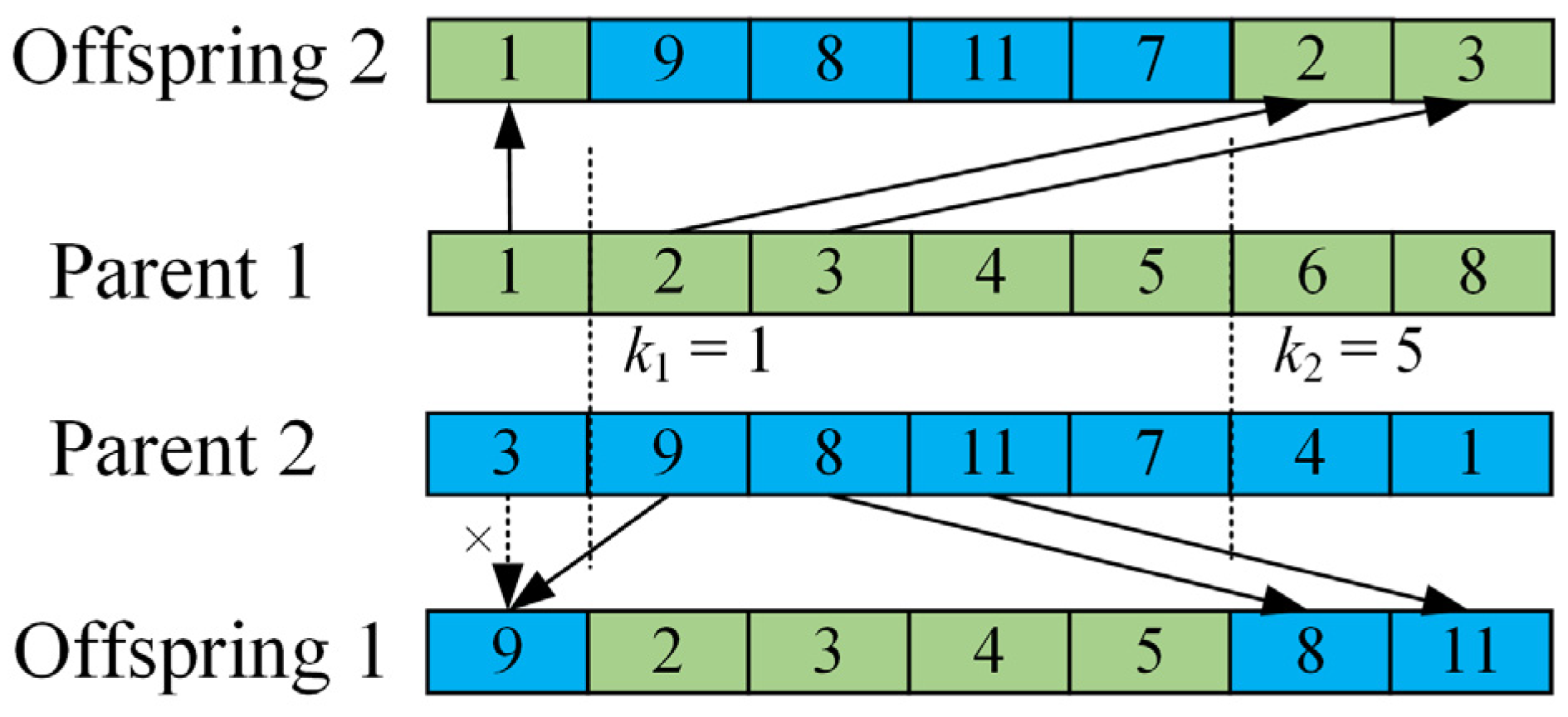
The process of the crossover operation is shown in Figure 2. Different colors represent gene segments from different parents. Arrows represent that the gene segments from the parents are retained in the offspring. Dashed arrows represent that the gene segments are not retained. For a pair of parent individuals, a random number r is generated from a uniform distribution within the range [0, 1]. The crossover probability p_c(g) is calculated according to Equation (25). If r < p_c(g), the crossover operation is performed; otherwise, it is skipped. For two parent individuals to perform a crossover operation, two crossover points k₁ and k₂ are randomly generated so that 1 < k₁ < k₂ < N_typ. A segment between k₁ and k₂ is extracted from Parent 1. Offspring 1 inherits this segment, and the remaining positions are filled in order with non-conflicting genes from Parent 2. Offspring 2 is generated symmetrically by reversing the roles of the parents.

(5)

Mutation operation for non-elite individuals

For each non-elite individual, a random number r is generated from a uniform distribution within the range [0, 1]. The mutation rate p_m(g) is calculated according to Equation (26). If r < p_m(g), the mutation operation is performed. For individuals undergoing mutation, a new index value is randomly selected from the set {1, 2, …, N_typ} that satisfies the uniqueness constraint of an individual (i.e., all elements in the individual are unique). The original gene at the selected position is then replaced with the new index value.

(6)

Iteration termination judgment

The new offspring individuals, including both elite and non-elite individuals after selection, crossover, and mutation, form the next-generation population. If the maximum number of evolution generations is reached, the optimization process is terminated and the solved typical scenarios are output; otherwise, the procedure returns to step 2.

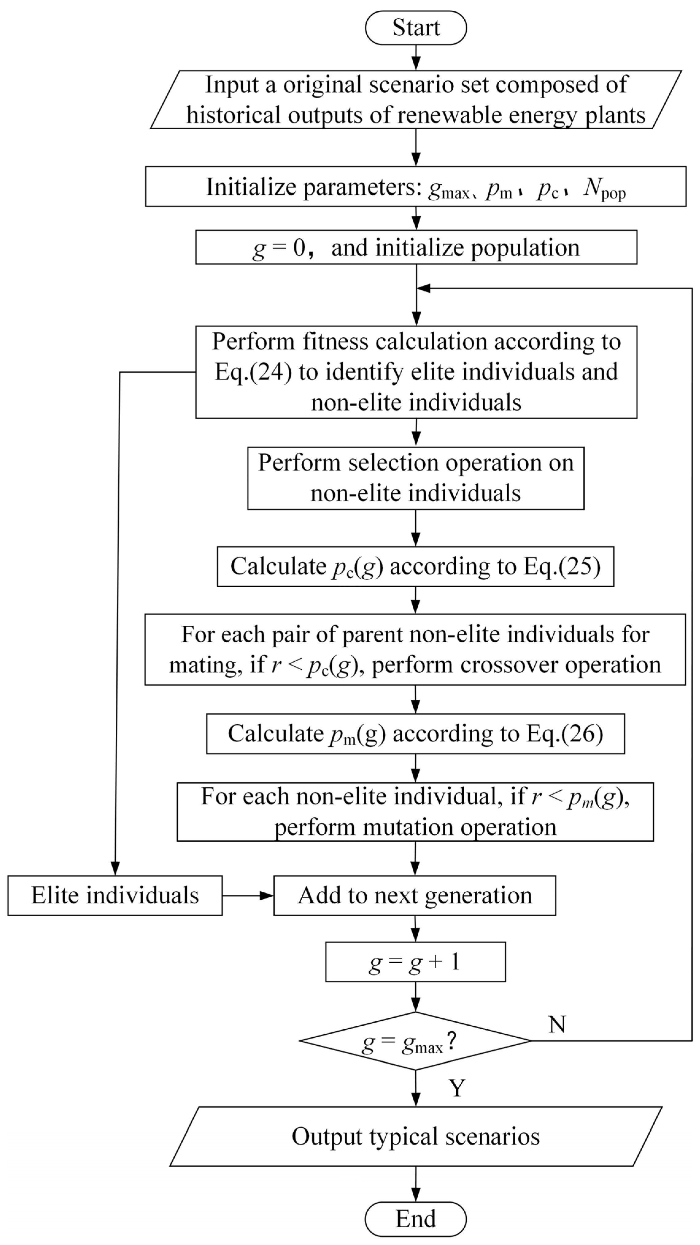
The solution flowchart of typical scenarios based on the improved genetic algorithm is shown in Figure 3.

The computational burden for solving typical scenarios increases as the size of the original scenario set grows. When dealing with large-scale original scenario sets, the solution process for typical scenarios becomes highly time-consuming. Due to the inherent compatibility of genetic algorithms with parallel computing techniques, the efficiency of extracting typical scenarios can be enhanced by increasing the number of parallel computation cores.

5. Case Study

The proposed construction method of typical scenarios is verified in multiple renewable energy plants in Belgium, including five wind farms (WFs) and fourteen photovoltaic (PV) plants. For scenario generation, historical output data from plants recorded over a period of one year serve as the original scenario set, including a total of 365 historical scenarios. The power outputs of all plants are normalized to eliminate potential large differences among different plants.

5.1. Scenario Reduction of Multiple WF Outputs

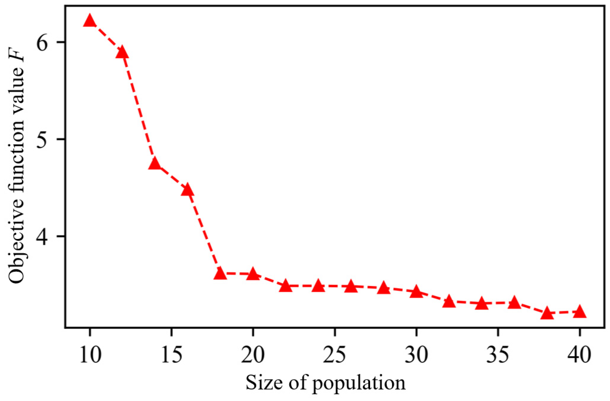
Typical scenarios for multiple WFs are solved using the improved genetic algorithm. Weighting coefficients α₁, α₂, α₃, and α₄ are set to 1. The number of typical scenarios N_typ is set to 4. The maximum iteration number g_max is set to 200. p_{c_max} is set to 0.8. p_{c_min} is 0.2. p_{m_max} is 0.4. p_{m_min} is 0.1. Objective function value F with different population sizes and N_e are shown in Figure A1 and Figure A2 in Appendix A. After the population size reaches 20, the optimization results no longer exhibit significant changes. Moreover, the optimal results are achieved when the number N_e of elite individuals is set to 2.

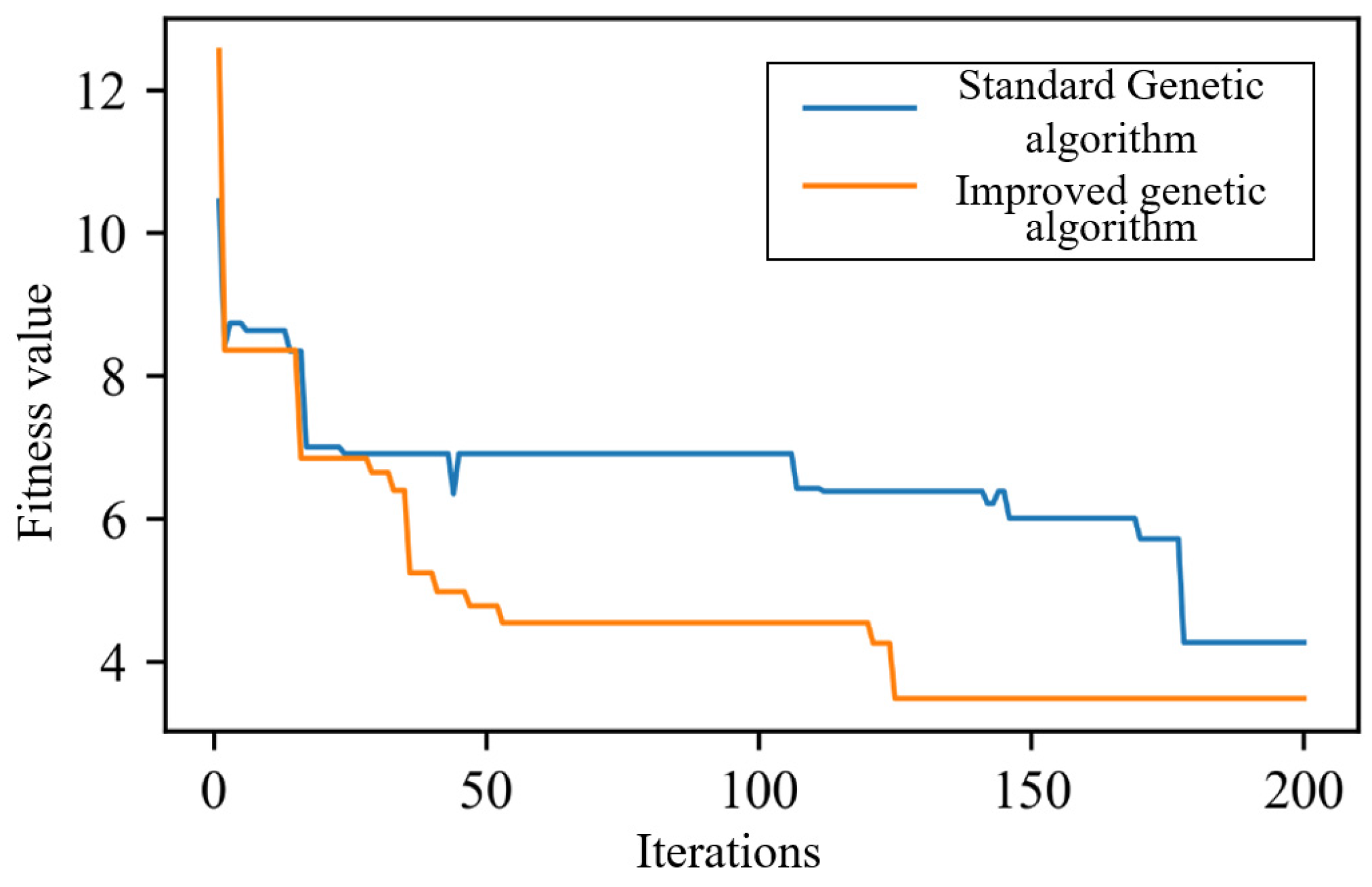
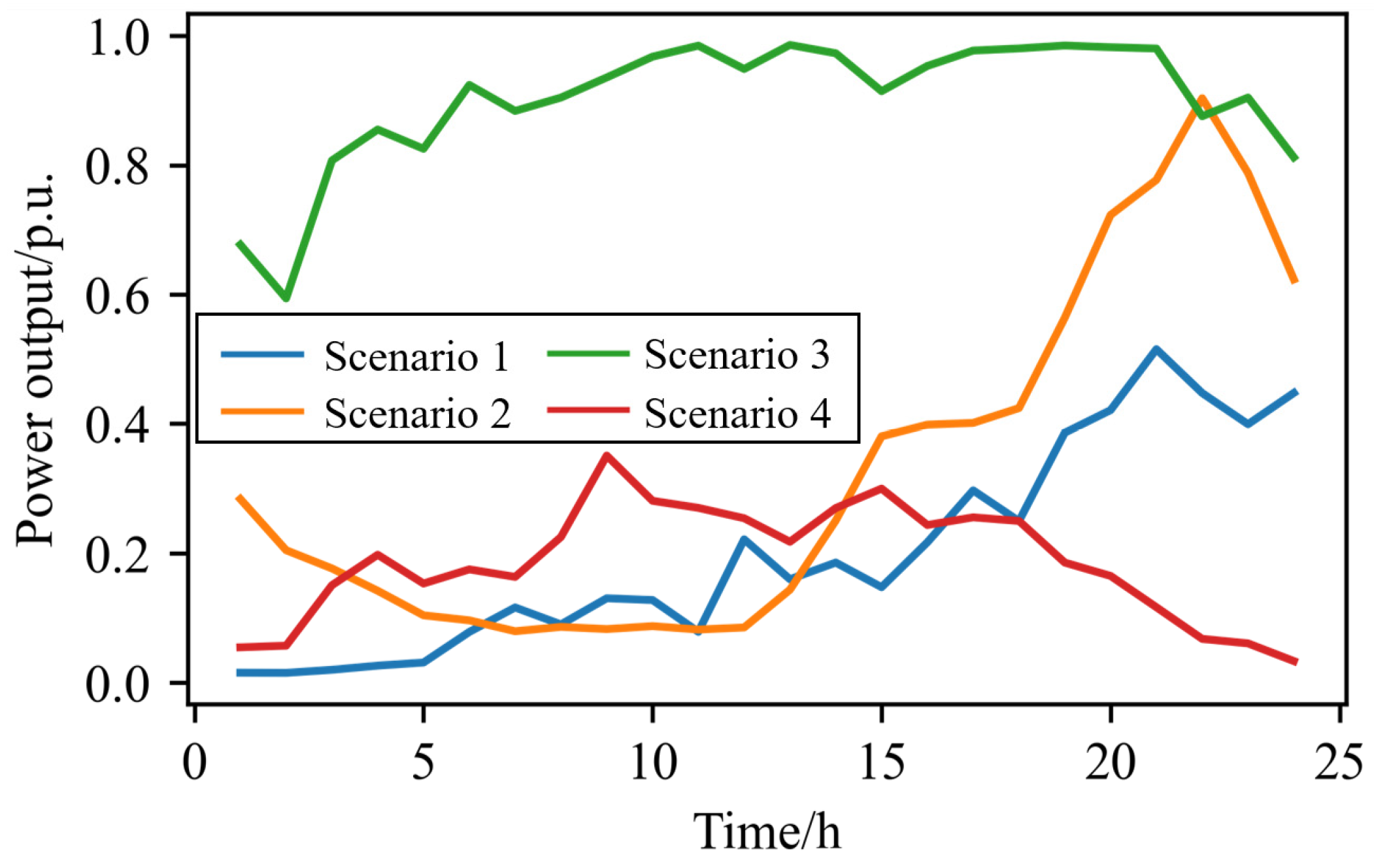
With a population size of 20 and N_e = 2, the fitness value variation curves of the improved and standard genetic algorithms during the optimization process are shown in Figure 4. The X-axis denotes the number of iterations in the genetic algorithm. The Y-axis fitness value is the objective function F. With 10 parallel computation cores, the standard genetic algorithm requires 177 iterations to obtain the optimal solution, which takes 234 s. The improved genetic algorithm achieves a higher-quality solution in just 125 iterations, which takes 165 s. Therefore, compared to the standard genetic algorithm, the improved genetic algorithm demonstrates faster convergence and superior solution quality. The four typical scenarios for WF 1 are shown in Figure 5. The X-axis denotes the sampling time points in one day. The Y-axis denotes the normalized power output of WF 1 on a single time point.

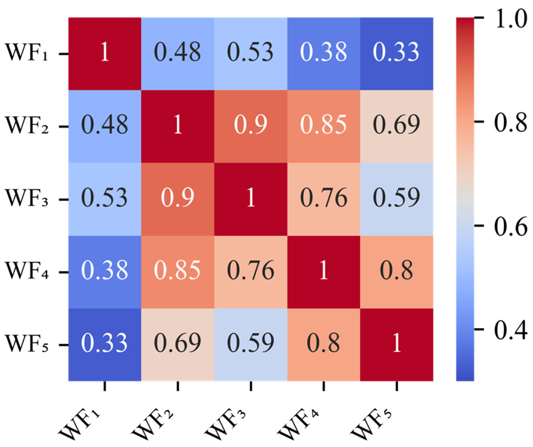
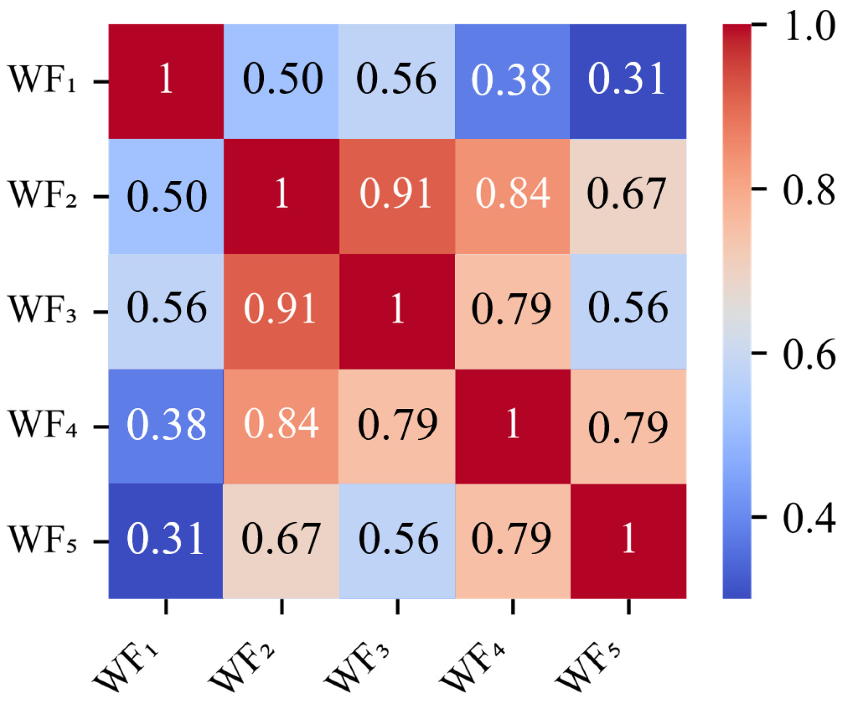
The mean and variance differences between original and typical scenarios across the five WFs are given in

Table 1. Means and variances between the original and typical scenario sets for five WFs.

	Original Scenario Set		Typical Scenario Set
	Mean/p.u.	Variance	Mean/p.u.	Variance
WF 1	0.4121	0.0308	0.4723	0.0319
WF 2	0.2455	0.0096	0.2765	0.0066
WF 3	0.2477	0.0089	0.2975	0.0092
WF 4	0.2374	0.0084	0.2532	0.0071
WF 5	0.1852	0.0087	0.1609	0.0081

. As shown in Table 1, the constructed typical scenario set maintains statistical similarity to the original scenario set in terms of mean and variance. Further comparisons of the spatial correlations of power outputs between the original and typical scenario sets are presented in Figure 6 and Figure 7. The numbers in Figure 6 and Figure 7 denote the spatial correlation coefficients between WF outputs.

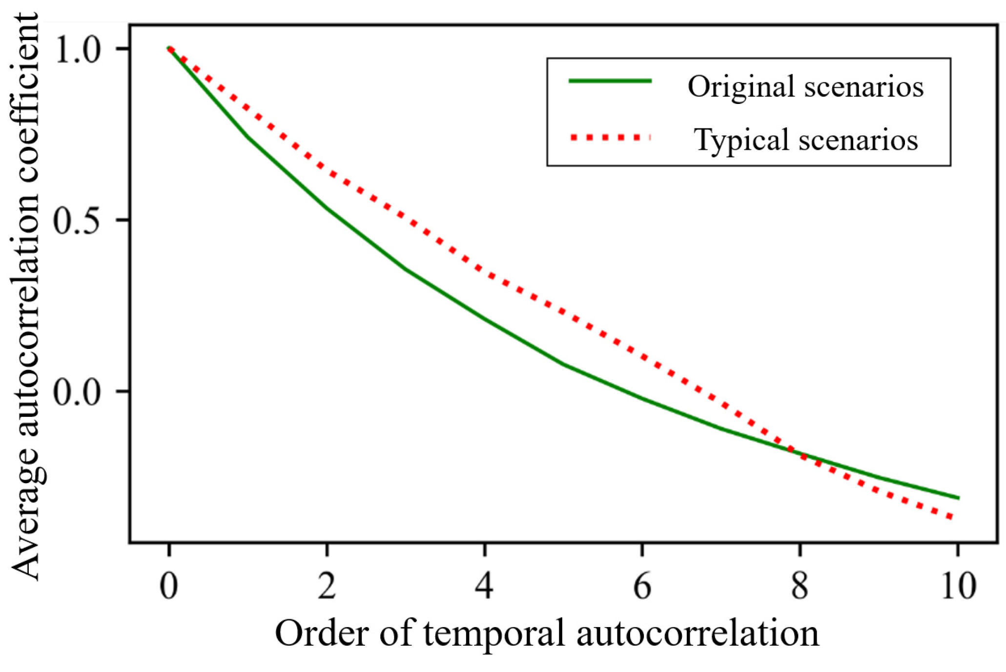
It can be seen that the spatial correlation heatmaps of power outputs across the five WFs in the original and typical scenario sets are highly similar. The mean absolute percentage error (MAPE) between spatial correlation matrices of the original and typical scenario sets is 2.5%, indicating that the obtained typical scenario set can effectively preserve the spatial correlations among multiple WFs. Furthermore, a comparison of the average temporal autocorrelation coefficient curves between the original and typical scenario sets for WF 1 is presented in Figure 8. The X-axis denotes the order of temporal autocorrelation. The Y-axis denotes the average autocorrelation coefficients of WF 1 across all scenarios. The percentage error between the first-order temporal autocorrelation coefficients of the original and typical scenario sets is 2.75%. The consistency between the two curves demonstrates that typical scenarios can also preserve the temporal autocorrelation of WF outputs.

5.2. Scenario Reduction of Multiple PV Plant Outputs

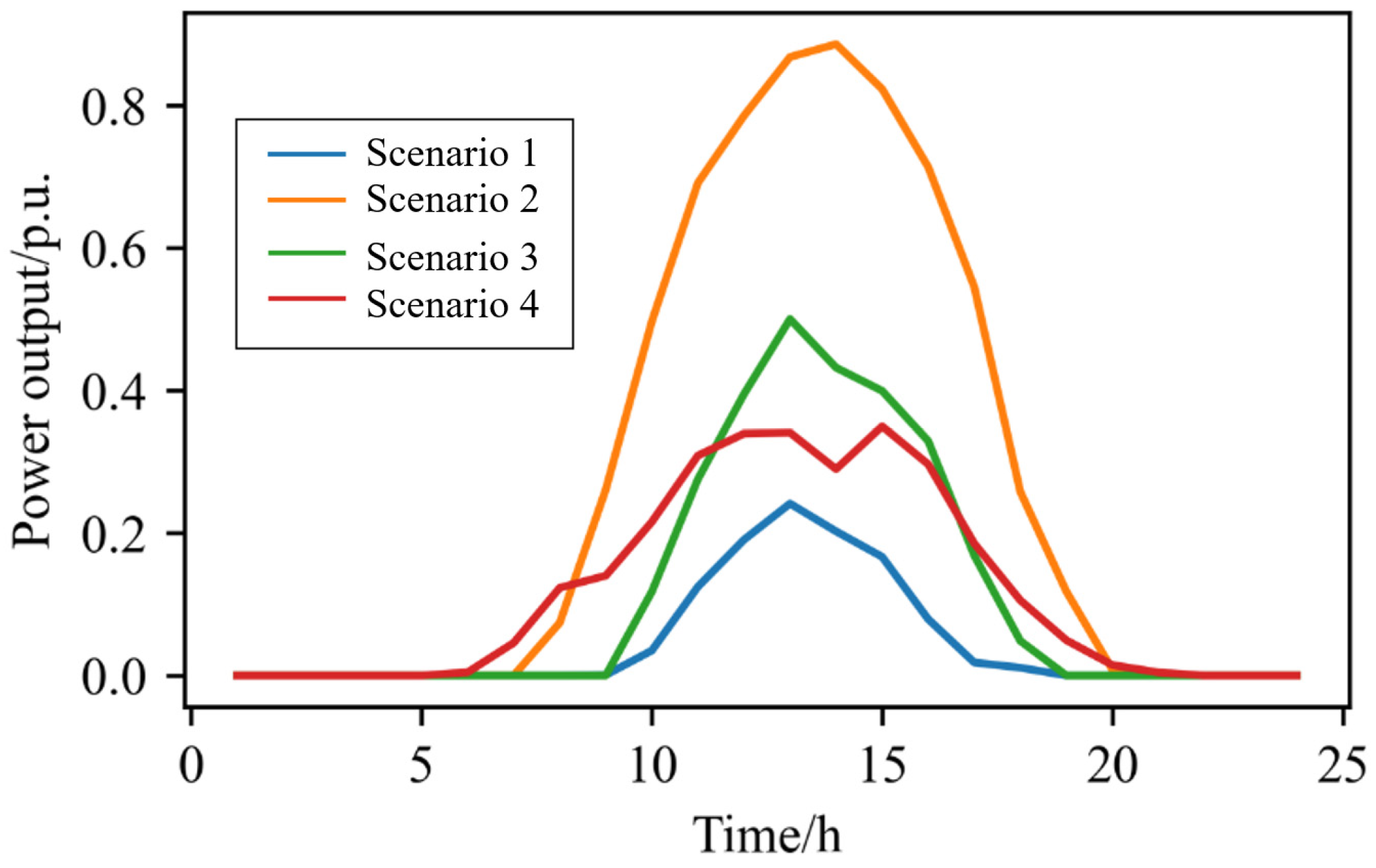
A typical scenario set for 14 PV plants is obtained using the improved genetic algorithm. Among these, the four typical output scenarios for PV plant 1 are shown in Figure 9. The Y-axis denotes the normalized power output of PV plant 1 on a single time point. It can be seen that the scenarios are distributed across distinct output intervals. The mean and variance differences between the original and typical scenario sets for the 14 PV plants are given in

Table 2. Means and variances between original and typical scenario sets for 14 PV plants.

	Original Scenario Set		Typical Scenario Set
	Mean/p.u.	Variance	Mean/p.u.	Variance
PV 1	0.1275	0.0358	0.1361	0.0415
PV 2	0.1268	0.0343	0.1347	0.0397
PV 3	0.1236	0.0335	0.13167	0.0390
PV 4	0.1335	0.0387	0.1410	0.0444
PV 5	0.1317	0.0372	0.1394	0.0430
PV 6	0.1315	0.0379	0.1420	0.0451
PV 7	0.1151	0.0285	0.1185	0.0311
PV 8	0.1265	0.0353	0.1376	0.0413
PV 9	0.1145	0.0287	0.1272	0.0343
PV 10	0.1090	0.0258	0.1235	0.0321
PV 11	0.1106	0.0268	0.1126	0.0271
PV 12	0.1138	0.0277	0.1221	0.0317
PV 13	0.1157	0.0293	0.1216	0.0329
PV 14	0.1383	0.0412	0.1413	0.0447

. The results indicate that the constructed typical scenario set retains mean and variance characteristics that are close to the original scenario set.

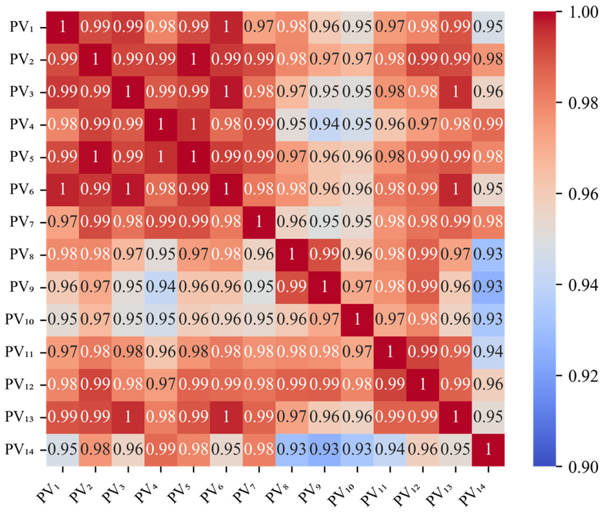
The spatial correlation heatmaps of power outputs among 14 PV plants in the original and typical scenario sets are shown in Figure 10 and Figure 11, respectively. The MAPE between spatial correlation matrices of the original and typical scenario sets is 0.78%. The high similarity in correlation distributions between the two sets indicates that the constructed typical scenario set can effectively capture the spatial correlations among the historical outputs of 14 PV plants. As shown in Figure 10 and Figure 11, the spatial correlation coefficients between PV plants are generally above 0.9. Compared to WFs, PV plants exhibit stronger spatial correlation. This is attributed to the large-scale, uniform, and gradual nature of solar irradiance variations, which lead to consistent power output changes among PV plants within the same region.

A further comparison of the average temporal autocorrelation coefficients between the original and typical scenario sets for PV plant 1 is shown in Figure 12. The Y-axis denotes the average autocorrelation coefficients of PV plant 1 across all scenarios. The percentage error between the first-order temporal autocorrelation coefficients of the original and typical scenario sets is 2.45%. The high degree of alignment between the two curves demonstrates that the constructed typical scenario set can effectively preserve the temporal autocorrelation of the historical outputs from PV plant 1.

In summary, the proposed construction method for typical scenarios for multiple renewable energy plant outputs based on the improved genetic algorithm can effectively preserve the statistical characteristics of the original scenario set, including the mean, variance, spatial correlation, and temporal correlation.

6. Conclusions

A construction method for typical scenarios considering spatiotemporal correlations among multiple renewable energy plant outputs is proposed in this paper. A symmetric spatial correlation matrix and a temporal autocorrelation matrix are defined, achieving quantitative representation of the spatiotemporal correlations. Distributional differences between the typical and original scenario sets are quantified in terms of mean, variance, spatial correlation, and temporal autocorrelation, and an optimization model for scenario reduction is constructed. The model is solved based on the improved genetic algorithm in order to obtain high-quality typical scenarios. The proposed method in this paper can provide typical scenarios that reflect distributional characteristics of original scenarios, thereby contributing to the optimality of the power grid planning schemes. The case study on multiple renewable energy plants in Belgium gives the following conclusions:

(1)

By incorporating adaptive parameter adjustment and an elitism strategy, the solution quality and efficiency of the improved genetic algorithm are enhanced significantly. Four high-quality typical scenarios can be obtained in 3 min.

(2)

The MAPE between spatial correlation matrices of the original and typical scenario sets for wind farms is 2.5%. The MAPE for photovoltaic plants is 0.78%. These simulation results demonstrate that the constructed typical scenarios can effectively capture the spatial correlations of the original scenarios.

(3)

The percentage error between first-order temporal autocorrelation coefficients of original and typical scenarios for wind farms is 2.75%. The MAPE for photovoltaic plants is 2.45%. The low errors demonstrate that typical scenarios can also capture the temporal correlations of the original scenarios.

While increasing the size of the typical scenario set can more accurately reflect the distributional characteristics of the original scenario set, it also increases the complexity of subsequent planning solutions. Future research should incorporate subsequent power grid planning solutions into the construction of typical scenarios, aiming to construct a minimal-sized typical scenario set that is well-suited for power grid planning.

References

1. Khaleel, M.; Yusupov, Z.; Rekik, S. Exploring trends and predictions in renewable energy generation. Energy 360 2025, 4, 100030. [Google Scholar] [CrossRef]
2. Wang, L.; Xie, L.; Yang, Y.; Zhang, Y.; Wang, K.; Cheng, S. Distributed online voltage control with fast PV power fluctuations and imperfect communication. IEEE Trans. Smart Grid 2023, 14, 3681–3695. [Google Scholar] [CrossRef]
3. Zhao, L.; Huang, Y.; Dai, Q.; Yang, L.; Chen, F.; Wang, L.; Sun, K.; Huang, J.; Lin, Z. Multistage active distribution network planning with restricted operation scenario selection. IEEE Access 2019, 7, 121067–121080. [Google Scholar] [CrossRef]
4. Li, H.; Ren, Z.; Fan, M.; Li, W.; Xu, Y.; Jiang, Y.; Xia, W. A review of scenario analysis methods in planning and operation of modern power systems: Methodologies, applications, and challenges. Electr. Power Syst. Res. 2022, 205, 107722. [Google Scholar] [CrossRef]
5. Stappers, B.; Paterakis, N.G.; Kok, K.; Gibescu, M. A class-driven approach based on long short-term memory networks for electricity price scenario generation and reduction. IEEE Trans. Power Syst. 2020, 35, 3040–3050. [Google Scholar] [CrossRef]
6. Gazijahani, F.S.; Salehi, J. Stochastic multi-objective framework for optimal dynamic planning of interconnected microgrids. IET Renew. Power Gener. 2017, 11, 1749–1759. [Google Scholar] [CrossRef]
7. Safdarian, A.; Fotuhi-Firuzabad, M.; Aminifar, F. Compromising wind and solar energies from the power system adequacy viewpoint. IEEE Trans. Power Syst. 2012, 27, 2368–2376. [Google Scholar] [CrossRef]
8. Chen, Y.; Wang, Y.; Kirschen, D.; Zhang, B. Model-free renewable scenario generation using generative adversarial networks. IEEE Trans. Power Syst. 2018, 33, 3265–3275. [Google Scholar] [CrossRef]
9. Yuan, R.; Wang, B.; Sun, Y.; Song, X.; Watada, J. Conditional style-based generative adversarial networks for renewable scenario generation. IEEE Trans. Power Syst. 2022, 38, 1281–1296. [Google Scholar] [CrossRef]
10. Song, Z.; Huang, Y.; Xie, H.; Li, X. Generation method of multi-regional photovoltaic output scenarios-set using conditional generative adversarial networks. IEEE J. Emerg. Sel. Top. Circuits Syst. 2023, 13, 861–870. [Google Scholar] [CrossRef]
11. Kang, M.; Zhu, R.; Chen, D.; Li, C.; Gu, W.; Qian, X.; Yu, W. A cross-modal generative adversarial network for scenarios generation of renewable energy. IEEE Trans. Power Syst. 2024, 39, 2630–2640. [Google Scholar] [CrossRef]
12. Dong, W.; Chen, X.; Yang, Q. Data-driven scenario generation of renewable energy production based on controllable generative adversarial networks with interpretability. Appl. Energy 2022, 308, 118387. [Google Scholar] [CrossRef]
13. Yao, W.; Huo, Z.; Zou, J.; Wu, C.; Wang, J.; Wang, X.; Lu, S.; Xie, Y.; Zhuo, Y.; Liang, J.; et al. Medium- and long-term power system planning method based on source-load uncertainty modeling. Energies 2024, 17, 5088. [Google Scholar] [CrossRef]
14. Suo, X.; Zhao, S.; Ma, Y. Multipoint layout planning method for multi-energy sources based on time-series production simulation. Int. J. Energy Res. 2022, 46, 9323–9344. [Google Scholar] [CrossRef]
15. Liu, D. An improved wind power scenario reduction method considering spatial-temporal correlation and cyber attacks. In Proceedings of the 3rd Asia Energy and Electrical Engineering Symposium (AEEES 2021), Chengdu, China, 26–29 March 2021; pp. 730–734. [Google Scholar]
16. Terrén-Serrano, G.; Ludkovski, M. Extreme day-ahead renewables scenario selection in power grid operations. Appl. Energy 2025, 391, 125747. [Google Scholar] [CrossRef]
17. Li, Z.; Li, Z. Linear programming-based scenario reduction using transportation distance. Comput. Chem. Eng. 2016, 88, 50–58. [Google Scholar] [CrossRef]
18. Sannigrahi, S.; Ghatak, S.R.; Acharjee, P. Multi-scenario based Bi-level coordinated planning of active distribution system under uncertain environment. IEEE Trans. Ind. Appl. 2019, 56, 850–863. [Google Scholar] [CrossRef]
19. Qiu, Y.; Li, Q.; Pan, Y.; Yang, H.; Chen, W. A scenario generation method based on the mixture vine copula and its application in the power system with wind/hydrogen production. Int. J. Hydrogen Energy 2019, 44, 5162–5170. [Google Scholar] [CrossRef]
20. Kile, H.; Uhlen, K.; Kjølle, G. Scenario selection in composite reliability assessment of deregulated power systems. Int. J. Electr. Power Energy Syst. 2014, 63, 124–131. [Google Scholar] [CrossRef]
21. Li, J.; Lan, F.; Wei, H. A scenario optimal reduction method for wind power time series. IEEE Trans. Power Syst. 2016, 31, 1657–1658. [Google Scholar] [CrossRef]
22. Zhou, H.; Wu, H.; Ye, C.; Xiao, S.; Zhang, J.; He, X.; Wang, B. Integration capability evaluation of wind and photovoltaic generation in power systems based on temporal and spatial correlations. Energies 2019, 12, 171. [Google Scholar] [CrossRef]
23. Tang, C.; Wang, Y.; Xu, J.; Sun, Y.; Zhang, B. Efficient scenario generation of multiple renewable power plants considering spatial and temporal correlations. Appl. Energy 2018, 221, 348–357. [Google Scholar] [CrossRef]
24. Poncelet, K.; Höschle, H.; Delarue, E.; Virag, A.; D’haeseleer, W. Selecting representative days for capturing the implications of integrating intermittent renewables in generation expansion planning problems. IEEE Trans. Power Syst. 2017, 32, 1936–1948. [Google Scholar] [CrossRef]
25. Zhu, N.; Wang, Y.; Yuan, K.; Yan, J.; Li, Y.; Zhang, K. GGNet: A novel graph structure for power forecasting in renewable power plants considering temporal lead-lag correlations. Appl. Energy 2024, 364, 123194. [Google Scholar] [CrossRef]
26. Raik, B. Generation of time-coupled wind power infeed scenarios using pair-copula construction. IEEE Trans. Sustain. Energy 2018, 9, 1298–1306. [Google Scholar]
27. Sharma, K.; Bhakar, R.; Tiwari, H.P.; Chawda, S. Scenario based uncertainty modeling of electricity market prices. In Proceedings of the 6th International Conference on Computer Applications in Electrical Engineering-Recent Advances (CERA 2017), Roorkee, India, 5–7 October 2017; pp. 164–168. [Google Scholar]
28. He, Y.; Wu, H.; Ding, M.; Bi, R.; Hua, Y. Reduction method for multi-period time series scenarios of wind power. Electr. Power Syst. Res. 2023, 214, 108813. [Google Scholar] [CrossRef]
29. Cheng, D.; Xing, F.; Su, R.; Qi, H.; Ma, L.; Ma, H.; Wang, T.; Zhou, N.; Li, C. Multiple wind farms power generation scenario generation and reduction based on multivariate copula function and greedy strategy. In Proceedings of the 7th International Conference on Power and Energy Engineering (ICPEE 2023), Chengdu, China, 22–24 December 2023; pp. 337–342. [Google Scholar]
30. Toaza, B.; Esztergaz-Kiss, D. A review of metaheuristic algorithms for solving TSP-based scheduling optimization problems. Appl. Soft Comput. 2023, 148, 110908. [Google Scholar] [CrossRef]
31. Shoaei, M.; Noorollahi, Y.; Hajinezhad, A.; Moosavian, S.F. A review of the applications of artificial intelligence in renewable energy systems: An approach-based study. Energy Convers. Manag. 2024, 306, 118207. [Google Scholar] [CrossRef]
32. Katoch, S.; Chauhan, S.S.; Kumar, V. A review on genetic algorithm: Past, present, and future. Multimed. Tools Appl. 2021, 80, 8091–8126. [Google Scholar] [CrossRef]
33. Hong, Y.; Nguyen, M. Multi-objective multi-scenario under-frequency load shedding in a standalone power system. IEEE Syst. J. 2020, 14, 2759–2769. [Google Scholar] [CrossRef]
34. Tang, L.; Dong, Y.; Liu, J. Differential evolution with an individual-dependent mechanism. IEEE Trans. Evol. Comput. 2015, 19, 560–574. [Google Scholar] [CrossRef]
35. Pandey, A.K.; Jadoun, V.K.; Jayalakshmi, N.S. Profit maximization based optimal scheduling of a virtual power plant using red fox optimizer. In Proceedings of the IEEE 10th Power India International Conference (PIICON 2022), New Delhi, India, 25–27 November 2022; pp. 1–6. [Google Scholar]
36. Pandey, A.K.; Jadoun, V.K.; Sabhahit, J.N.; Sharma, S. Interconnected operation and economic feasibility-based sustainable planning of virtual power plant in multi-area context. Smart Cities 2025, 8, 37. [Google Scholar] [CrossRef]
Figure 1. Diagram of the elitism-based evolutionary strategy.
Symmetry 17 01226 g001
Figure 2. Schematic diagram of crossover operation.
Symmetry 17 01226 g002
Figure 3. Flowchart of scenario reduction based on an improved genetic algorithm.
Symmetry 17 01226 g003
Figure 4. The fitness variation curves of the standard and improved genetic algorithms.
Symmetry 17 01226 g004
Figure 5. Typical scenario set for WF 1.
Symmetry 17 01226 g005
Figure 6. Heatmap of spatial correlations in the original scenario set for five WFs.
Symmetry 17 01226 g006
Figure 7. Heatmap of spatial correlations in the typical scenario set for five WFs.
Symmetry 17 01226 g007
Figure 8. Average autocorrelation coefficients of original and typical scenarios for WF 1.
Symmetry 17 01226 g008
Figure 9. Typical scenario set for PV plant 1.
Symmetry 17 01226 g009
Figure 10. Heatmap of spatial correlations in the original scenario set for 14 PV plants.
Symmetry 17 01226 g010
Figure 11. Heatmap of spatial correlations in the typical scenario set for 14 PV plants.
Symmetry 17 01226 g011
Figure 12. Average autocorrelation coefficients between the original and typical scenario sets for PV plant 1.
Symmetry 17 01226 g012