A Qualitative Analysis and Discussion of a New Model for Optimizing Obesity and Associated Comorbidities

Abstract

This paper addresses the problem of optimizing obesity, which has been a challenging issue in the last decade based on recent data revealed in 2024 by the World Health Organization (WHO). The current work introduces a new mathematical model of the dynamics of weight over time with embedded control parameters to optimize the number of obese, overweight, and comorbidity populations. The mathematical formulation of the model is developed under certain sufficient conditions that guarantee the positivity and boundedness of solutions over time. The model structure exhibits inherent symmetry in population group transitions, particularly around the equilibrium state, which allows the application of analytical tools such as the Routh–Hurwitz and Metzler criteria. Then, the analysis of local and global stability of the obesity-free equilibrium state is discussed based on these criteria. Based on the Pontryagin maximum principle (PMP), the deviation from the obesity-free equilibrium state is controlled. The model’s effectiveness is demonstrated through simulation using the Forward–Backward Sweeping algorithm with parameters derived from recent research in human health. Incorporating symmetry considerations in the model enhances the understanding of system behavior and supports balanced intervention strategies. Results suggest that the model can effectively inform strategies to mitigate obesity prevalence and associated health risks.

1. Introduction

Obesity is a chronic and multifaceted condition characterized by an excessive accumulation of body fat, which can have significant health implications. It is commonly assessed using the body mass index (BMI), calculated by dividing a person’s weight in kilograms by the square of their height in meters (kg/m²). A BMI of 30 or higher is typically considered indicative of obesity.

Obesity is becoming a major global public health concern due to its significant influence on health outcomes and its contribution to the increased incidence of noncommunicable diseases (NCDs) such as diabetes, cardiovascular disease, and various types of cancer.

The development of obesity is a multifaceted condition that can be impacted by a range of factors, including genetics, hormones, metabolism, psychology, socioeconomic status, and access to unhealthy food, as well as a lack of physical activity. Obesity is frequently associated with other health conditions like type 2 diabetes, heart disease, high blood pressure, sleep disorders, and certain cancers. It can also affect mental and social health, resulting in problems such as low self-esteem, depression, and societal discrimination.

According to projections based on data from the World Obesity Atlas (WOT) and World Health Organization (WHO) in 2023, it is expected that over half of the world’s population will be classified as overweight or obese with a BMI ≥ 25 kg/m² by 2035, compared to $38\%$ in 2020 [1,2]. The expectations also refer to 2 billion people of all ages, with a percentage of $24\%$ being obese with a BMI ≥ 30 kg/m² in 2035, compared to $14\%$ in 2020.

The issue of obesity is a growing concern in the Gulf Cooperation Council (GCC) nations, particularly in Saudi Arabia (SA), where there has been a notable rise in obesity rates among adults and children [3]. Factors such as rapid urbanization, a shift towards processed and high-calorie diets, and a more sedentary lifestyle are contributing to the increasing prevalence of obesity in the GCC countries. The adoption of a Westernized diet high in carbohydrates and fats has replaced traditional eating habits, leading to an imbalance in energy consumption. Additionally, changes in urban lifestyles, including reduced physical activity and increased time spent on social media, are exacerbating the issue [4,5,6]. These changes have significant implications, putting strain on the national healthcare system and presenting health challenges for individuals.

A recent study conducted by Althumiri et al. [4] included 4709 participants, comprising 2358 females ($50.1\%$) and 2351 males ($48.9\%$), aged 18 years and above, from 13 different regions in SA. The study found that 1023 participants (601 females and 422 males) were classified as obese, with an overall prevalence of $21.7\%$ ($25.5\%$ among females and $17.9\%$ among males).

Table 1. Number of obese participants in the sample being studied based on place of residence in SA [4].

District	No. of Obese Participants	Ratio
Madinah	84 out of 366	$23.0\%$
Baha	52 out of 364	$14.3\%$
Jazan	72 out of 361	$19.9\%$
Eastern Region	106 out of 360	$29.4\%$
Jouf	96 out of 361	$26.6\%$
Hail	72 out of 359	$20.1\%$
Asir	66 out of 366	$18.0\%$
Qassim	66 out of 361	$18.3\%$
Riyadh	98 out of 364	$26.9\%$
Mecca	92 out of 362	$25.4\%$
Tabuk	70 out of 362	$19.3\%$
Northern Borders	76 out of 361	$21.1\%$
Najran	73 out of 362	$20.2\%$

and

Table 2. Number of obese participants in the sample being studied based on age group (years) in SA [4].

Age Group	No. of Obese Participants	Ratio
18–19	36 out of 255	$14.1\%$
20–29	231 out of 1556	$14.8\%$
30–39	183 out of 1009	$18.1\%$
40–49	311 out of 1044	$29.8\%$
50–59	182 out of 555	$32.8\%$
60+	80 out of 290	$27.6\%$

present the distribution of obese participants based on their region of residence and age group, respectively [4]. The authors emphasized the rising incidence of non-communicable diseases (NCDs) linked to obesity in SA and warned that the future health of the population could be jeopardized without interventions to promote healthier dietary habits, increase physical activity, and enhance community education. Addressing this issue effectively requires a comprehensive approach involving targeted policies and community programs to reduce obesity rates and alleviate its impact on public health and health care costs in SA. Furthermore, Alsulami et al. [7] examined the prevalence of obesity, physical activity, and dietary habits among adults in the Makkah region of SA through a cross-sectional survey and the validated Arab Teens Lifestyle Study (ATLS) questionnaire. The study revealed that $41\%$ and $38\%$ of male and female participants were overweight, respectively, while $23.1\%$ and $24.2\%$ were obese as depicted in Figure 1. Higher obesity rates were associated with older age, lower physical activity in both males and females, and increased consumption of fast food and sugary beverages. These findings underscore the critical need for targeted public health interventions focusing on lifestyle changes to combat obesity in the region.

To analyze obesity dynamics and evaluate preventive measures at individual and population levels, mathematical modeling is a valuable tool. Jódar et al. [8] utilized epidemiological modeling to demonstrate the significant impact of dietary patterns, particularly the consumption of energy-dense processed foods, on the transmission of childhood obesity. Building on these findings, Santonja et al. [9] conducted a population-level study on adult obesity dynamics, highlighting physical inactivity and inadequate nutrition as key factors. Their model projections indicated a continued increase in obesity prevalence without intervention. Furthermore, advanced mathematical frameworks have revolutionized our understanding of the multifaceted causes of obesity. Ejima et al. [10] identified social contagion as the primary driver of obesity spread, developing a novel transgenerational mathematical model that differentiated between genetic predisposition and social transmission factors. Al-Tuwairqi et al. [11] further enhanced this research with a nonlinear dynamical system that predicted population-level obesity trends across various behavioral scenarios, incorporating exercise adherence rates and peer influence effects. Additionally, mathematical modeling enables researchers to determine pathophysiological relationships between obesity and other illnesses. Carrillo et al. [12,13] developed a coupled obesity–cancer model that evaluated how weight loss improved treatment efficacy by solving an optimal control problem combining nutritional therapies and chemotherapy protocols. Similarly, Siewe et al. [14] created a glucose homeostasis model that evaluated the risk of diabetes by formulating insulin resistance brought on by fat as a disruption of the control system. By resolving a multi-objective optimal control problem that simultaneously improved tumor suppression and metabolic health in obese individuals, Dehingia et al. [15] made significant progress in this field with the help of optimization strategies that enabled a more accurate assessment of intervention strategies. Aldila et al. [16] utilized a compartmental model with time-dependent control variables to solve the optimal control problem and identify cost-effective methods for reducing prevalence. Fatima et al. [17] developed an objective functional to determine the best education and treatment protocols, balancing intervention costs with health outcomes using Pontryagin’s maximum principle. Their results indicated that early prevention strategies yielded greater long-term benefits compared to delayed treatment-focused measures.

This study develops a new mathematical model to represent the dynamics of body weight over time. Building on the classification in [7], obesity is divided into three distinct categories: class 1 obesity ($30\le \mathrm{BMI}<35$ kg/m²), class 2 obesity ($35\le \mathrm{BMI}<40$ kg/m²), and class 3 obesity (BMI $\ge 40$ kg/m²). The model also introduces a comorbidity compartment, enabling the analysis of obesity-related complications by incorporating comorbidity-induced mortality. This addition is important because obesity typically does not lead to direct mortality; rather, it contributes to the development of serious comorbidities, which can significantly increase the risk of death. As noted by [18], common comorbid conditions include type 2 diabetes mellitus, hypertension, cardiovascular disease, obstructive sleep apnea, gallstones, hyperlipidemia, fatty liver disease, osteoarthritis, psychosocial disorders, and infertility.

The remainder of this paper is organized as follows. The mathematical model is formulated in Section 2. Section 3 discusses the positivity and boundedness of the model’s solutions over time, as well as the stability of the obesity-free equilibrium using both the Routh–Hurwitz and Metzler criteria. Section 4 applies the Pontryagin maximum principle (PMP) to identify optimal strategies for reducing deviations from the obesity-free equilibrium. In Section 5, the model’s effectiveness is evaluated through numerical simulations using the Forward–Backward Sweeping algorithm. Finally, the conclusions and suggested directions for future work are presented in Section 6.

2. Model Formulation

Using compartmental models, we formulate a system of differential equations that will aid in assessing the impact of obesity mitigation strategies. We adopt the BMI classification from the CDC, https://www.cdc.gov/bmi/adult-calculator/bmi-categories.html, accessed on 23 November 2024. Body mass index (BMI) is determined by dividing an individual’s weight in kilograms by the square of their height in meters. For people aged 20 years and above, BMI categories apply uniformly, without considering age, sex, or race. In this study, we classified the population based on BMI as follows: underweight (below 18.5), healthy weight (18.5 to under 25), overweight (25 to under 30), and obese (30 or higher). We further classify the obesity class as follows, class 1 obesity (30 to less than 35), class 2 obesity (35 to less than 40), and class 3 obesity (severe obesity—40 or greater). This classification was used in the population compartmentalization of the model. Hence, the model was divided into the following populations:

$$N\left(t\right)=H\left(t\right)+V\left(t\right)+O_1\left(t\right)+O_2\left(t\right)+O_3\left(t\right)+C\left(t\right),$$

(1)

where $N\left(t\right)$ represents the total population, $H\left(t\right)$ represents the healthy population, $V\left(t\right)$ the overweight population, $O_1\left(t\right)$ the class 1 obesity, $O_2\left(t\right)$ the class 2 obesity, $O_3\left(t\right)$ the class 3 obesity, and $C\left(t\right)$ represents the population with comorbidities.

In the formulation of the model, the following assumptions were made:

• A constant recruitment rate of $\pi$.
• Obesity dynamics follow the BMI classification.
• Death is due to natural mortality and comorbidity induction.
• Populations are mixing homogeneously.

Based on the assumptions above and the flow diagram in Figure 2, we formulated the following system of differential equations:

$$\begin{array}{cc}\hfill {\displaystyle \frac{dH}{dt}}& ={\pi }_N+{\tau }_{v}V-({\beta }_v+\mu )H,\hfill \\ \hfill {\displaystyle \frac{dV}{dt}}& ={\beta }_{v}H+{\tau }_1{O}_1-(d_v+{\beta }_1+{\tau }_v+\mu )V,\hfill \\ \hfill {\displaystyle \frac{d{O}_1}{dt}}& ={\beta }_{1}V+{\tau }_2{O}_2-({\beta }_2+{\tau }_1+d_1+\mu )O_1,\hfill \\ \hfill {\displaystyle \frac{d{O}_2}{dt}}& ={\beta }_2{O}_1+{\tau }_3{O}_3-({\beta }_3+{\tau }_2+d_2+\mu )O_2,\hfill \\ \hfill {\displaystyle \frac{d{O}_3}{dt}}& ={\beta }_3{O}_2-({\tau }_3+d_3+\mu )O_3,\hfill \\ \hfill {\displaystyle \frac{dC}{dt}}& =d_{v}V+d_1{O}_1+d_2{O}_2+d_3{O}_3-(\mu +\delta )C.\hfill \end{array}$$

(2)

The description of the model parameters are given in

Table 3. Parameters (units: year⁻¹).

Parameter	Meaning	Value	Source
$\pi$	Recruitment rate	0.01335	[19]
${\beta }_v$	Rate of becoming overweight	0.13	[20]
${\beta }_1$	Rate of becoming obese stage 1	0.14	[20]
${\beta }_2$	Rate of becoming obese stage 2	0.16	Assumed
${\beta }_3$	Rate of becoming obese stage 3	0.18	Assumed
$d_v$	Comorbidity acquisition rate for overweight	0.0392	[21]
$d_1$	Comorbidity acquisition rate for obese stage 1	0.33	[22]
$d_2$	Comorbidity acquisition rate for obese stage 2	0.38	[22]
$d_3$	Comorbidity acquisition rate for obese stage 3	0.44	[22]
${\tau }_v$	Treatment rate for overweight	0.09	[23]
${\tau }_1$	Treatment rate for obese stage 1	0.08	[23]
${\tau }_2$	Treatment rate for obese stage 2	0.07	Assumed
${\tau }_3$	Treatment rate for obese stage 3	0.06	Assumed
$\delta$	Comorbidity-induced mortality rate	0.1225	[24]
$\mu$	Natural mortality rate	0.03	[19]

.

Remark 1.

The parameters ${\beta }_2$, ${\beta }_3$, ${\tau }_2$, and ${\tau }_3$ in Table 3 were not directly derived from empirical data but estimated based on logical extensions of known physiological trends and on the published literature. The rationale for these estimations is outlined below:

1. 

The parameters ${\beta }_2$ and ${\beta }_3$ were assumed relative to ${\beta }_1$, with the understanding that progression to more severe obesity stages tends to accelerate as BMI increases. This aligns with findings that individuals in higher obesity classes are more susceptible to further weight gain and associated complications [25].

2. 

The treatment rates ${\tau }_2$ and ${\tau }_3$ were assumed to be lower than ${\tau }_1$, reflecting the clinical observation that weight loss becomes increasingly difficult to achieve and maintain at higher obesity stages. Individuals with more severe obesity often face greater biological and behavioral challenges to effective treatment [26].

3. 

A sensitivity analysis was conducted to assess how variations in the estimated parameters affected the model’s behavior. Figures 6–9 and data summarized in Table 5 illustrate that the model remained stable and responsive under changes in these assumptions, supporting the reliability of the results.

3. Key Characteristics of the Proposed Model

3.1. Positivity and Boundedness of the Proposed Model

For realistic modeling of human population, all the state variables must be positive, and the solutions to the model system with positive initial conditions should remain positive, yielding the following theorem.

Theorem 1.

For the given initial conditions of model (2), the solutions of our model’s system remains positive for all $t>0$.

Proof. 

Healthy population: Taking the equation for the healthy and assuming there is no disease,

$$\begin{gathered} {\displaystyle \frac{dH}{dt}}={\pi }_N+{\tau }_{v}V-({\beta }_v+\mu )H,\Rightarrow {\displaystyle \frac{dH}{dt}}\ge -{\varphi }_{h}H, \\ \Rightarrow {\displaystyle \frac{dH}{H}}\ge -{\varphi }_{h}dt,\Rightarrow \ln \left|H\right|\ge -{\varphi }_{h}t+c_1. \end{gathered}$$

for constant $c_1$ and ${\varphi }_h={\beta }_v+\mu$. Taking the exponential of both sides,

$$\begin{array}{c}\hfill e^{\ln \left|H\right|}\ge e^{-{\varphi }_{h}t+c_1}=K{e}^{-{\varphi }_{h}t},\Rightarrow H\left(t\right)\ge K{e}^{-{\varphi }_{h}t}.\end{array}$$

where $K=e^{c_1}$ is a constant. Substituting the initial condition $H\left(0\right)=H_0$,

$$\begin{array}{c}\hfill H\left(0\right)\ge K{e}^{-{\varphi }_h\left(0\right)}=H_0,\Rightarrow H\left(t\right)\ge H_0{e}^{-{\varphi }_{h}t}.\end{array}$$

Hence, $K=H_0$. The exponential part is always positive, and $H_0\ge 0$, hence $H\left(t\right)$ is always positive, meaning $H\left(t\right)\ge 0$. In the same way, all our states are positive,

$$\begin{array}{cc}\hfill V\left(t\right)& \ge V_0{e}^{-{\varphi }_{v}t},O_1\left(t\right)\ge O_{10}{e}^{-{\varphi }_{1}t},O_2\left(t\right)\ge O_{20}{e}^{-{\varphi }_{2}t},\hfill \\ \hfill O_3\left(t\right)& \ge O_{30}{e}^{-{\varphi }_{3}t},C\left(t\right)\ge C_0{e}^{-{\varphi }_{c}t}.\hfill \end{array}$$

given the initial conditions $V_0,O_{10},O_{20},O_{30}$ and $C_0$. □

Boundedness ensures population sizes within each compartment cannot grow indefinitely or exceed a reasonable and feasible range. This yields the following theorem.

Theorem 2.

The solutions of model (2) with the initial conditions given are bounded in a positive region Ω.

Proof. 

$$\begin{array}{cc}\hfill {\displaystyle \frac{dN}{dt}}& ={\displaystyle \frac{dH}{dt}}+{\displaystyle \frac{dV}{dt}}+{\displaystyle \frac{d{O}_1}{dt}}+{\displaystyle \frac{d{O}_2}{dt}}+{\displaystyle \frac{d{O}_3}{dt}}+{\displaystyle \frac{dC}{dt}},\hfill \\ \hfill {\displaystyle \frac{dN}{dt}}& ={\pi }_N+{\tau }_{v}V-({\beta }_v+\mu )H+{\beta }_{v}H+{\tau }_1{O}_1-(d_v+{\beta }_1+{\tau }_v+\mu )V\hfill \\ \hfill & +{\beta }_{1}V+{\tau }_2{O}_2-({\beta }_2+{\tau }_1+d_1+\mu )O_1+{\beta }_2{O}_1+{\tau }_3{O}_3-({\beta }_3+{\tau }_2+d_2+\mu )O_2\hfill \\ \hfill & +{\beta }_3{O}_2-({\tau }_3+d_3+\mu )O_3+d_{v}V+d_1{O}_1+d_2{O}_2+d_3{O}_3-(\mu +\delta )C,\hfill \\ \hfill {\displaystyle \frac{dN}{dt}}& ={\pi }_N-\delta C-(H+V+O_1+O_2+O_3+C)\mu ,\hfill \\ \hfill {\displaystyle \frac{dN}{dt}}& ={\pi }_N-\delta C-\mu N,\hfill \end{array}$$

since $N=H+V+O_1+O_2+O_3+C$. Assuming there is no disease in the system,

$$\begin{array}{cc}\hfill {\displaystyle \frac{dN}{dt}}& \le {\pi }_N-\mu N.\hfill \end{array}$$

Solving the above inequality using the integrating factor method and applying the initial condition $N\left(0\right)=N_0$,

$$\begin{array}{cc}\hfill N\left(t\right)& \le {\displaystyle \frac{{\pi }_N}{\mu }}+(N_0-{\displaystyle \frac{{\pi }_N}{\mu }})e^{-\mu t}.\hfill \end{array}$$

If $N_0>{\displaystyle \frac{{\pi }_N}{\mu }}$, the right-hand side (RHS) experiences the largest possible value of $N_0$. That is, $N\left(t\right)\le N_0$ for all $t>0$. If $N_0<{\displaystyle \frac{{\pi }_N}{\mu }}$, the largest possible value of the RHS approaches ${\displaystyle \frac{{\pi }_N}{\mu }}$ as time t goes to infinity $N_0$. That is, $N\left(t\right)\le N_0$ for all $t>0$. Hence, $N\left(t\right)\le \max \{N_0,{\displaystyle \frac{{\pi }_N}{\mu }}\}$∀$t>0$, thus $\Omega$ □

The obesity-free equilibrium point (${\widehat{E}}_0$) is obtained by setting the system of differential equations to zero and setting all infected classes to zero. ${\widehat{E}}_0$ is given by

$${\widehat{E}}_0=\left({\displaystyle \frac{{\pi }_N}{\mu }},0,0,0,0,0\right).$$

The endemic equilibrium ($EE$) is obtained by setting the system of differential equations to zero and solving for each variable. $EE$ is given by

$$EE=\widehat{E}=(\widehat{H},\widehat{V},{\widehat{O}}_1,{\widehat{O}}_2,{\widehat{O}}_3,\widehat{C})$$

where

$$\begin{array}{cc}\hfill \widehat{H}& ={\displaystyle \frac{{\pi }_N+{\tau }_v\widehat{V}}{({\beta }_v+\mu )}},\widehat{V}={\displaystyle \frac{{\beta }_v\widehat{H}+{\tau }_1{\widehat{O}}_1}{d_v+{\beta }_1+{\tau }_v+\mu }},{\widehat{O}}_1={\displaystyle \frac{{\beta }_1\widehat{V}+{\tau }_2{\widehat{O}}_2}{{\beta }_2+{\tau }_1+d_1+\mu }},\hfill \\ \hfill {\widehat{O}}_2& ={\displaystyle \frac{{\beta }_2{\widehat{O}}_1+{\tau }_3{\widehat{O}}_3}{({\beta }_3+{\tau }_2+d_2+\mu )}},{\widehat{O}}_3={\displaystyle \frac{{\beta }_3{\widehat{O}}_2}{{\tau }_3+d_3+\mu }},\widehat{C}={\displaystyle \frac{d_v\widehat{V}+d_1{\widehat{O}}_1+d_2{\widehat{O}}_2+d_3{\widehat{O}}_3}{(\mu +\delta )}}.\hfill \end{array}$$

3.2. Local Stability Analysis of the Obesity-Free Equilibrium State

The general Jacobian matrix, $J_{E_0}$, of the proposed model after substituting $E_0$ is written as

$$J_{E_0}=\left[\begin{array}{cccccc}-({\beta }_v+\mu )& {\tau }_v& 0& 0& 0& 0\\ 0& -v_1& {\tau }_1& 0& 0& 0\\ 0& {\beta }_1& -v_2& {\tau }_2& 0& 0\\ 0& 0& {\beta }_2& -v_3& {\tau }_3& 0\\ 0& 0& 0& {\beta }_3& -v_4& 0\\ 0& d_v& d_1& d_2& d_3& -(\delta +\mu )\end{array}\right],$$

where $v_1={\beta }_1+d_v+{\tau }_v+\mu ,v_2={\beta }_2+d_1+{\tau }_1+\mu ,v_3={\beta }_3+d_2+{\tau }_2+\mu$, and $v_4=d_3+{\tau }_3+\mu$. By inspection of $J_{E_{0(1,1)}}$ and $J_{E_{0(6,6)}}$, negative eigenvalues ${\lambda }_1=-({\beta }_v+\mu )$ and ${\lambda }_2=-(\delta +\mu )$ are obtained. The matrix reduces to

$$J_{E_0}=\left[\begin{array}{cccc}-v_1& {\tau }_1& 0& 0\\ {\beta }_1& -v_2& {\tau }_2& 0\\ 0& {\beta }_2& -v_3& {\tau }_3\\ 0& 0& {\beta }_3& -v_4\end{array}\right].$$

(3)

From Remark 3, the corresponding characteristic polynomial is given by:

$$\begin{array}{cc}\hfill P\left(\lambda \right)& ={\lambda }^4+(v_1+v_2+v_3+v_4){\lambda }^3\hfill \\ \hfill & +\left(-{\beta }_1{\tau }_1-{\beta }_2{\tau }_2-{\beta }_3{\tau }_3+v_1{v}_2+v_2{v}_3+v_2{v}_4+v_1{v}_3+v_1{v}_4+v_3{v}_4\right){\lambda }^2\hfill \\ \hfill & +\left[-{\beta }_1{\tau }_1(v_3+v_4)-{\beta }_2{\tau }_2(v_1+v_4)-{\beta }_3{\tau }_3(v_1+v_2)\right.\hfill \\ \hfill & \left.+v_1{v}_3(v_2+v_4)+v_2{v}_4(v_3+v_1)\right]\lambda \hfill \\ \hfill & +v_1{v}_2{v}_3{v}_4+{\beta }_1{\beta }_3{\tau }_1{\tau }_3-{\beta }_1{\tau }_1{v}_3{v}_4-{\beta }_2{\tau }_2{v}_1{v}_4-{\beta }_3{\tau }_3{v}_1{v}_2.\hfill \end{array}$$

(4)

Based on the Routh–Hurwitz criterion, a 4th-degree polynomial

$$P\left(\lambda \right)={\lambda }^4+a_1{\lambda }^3+a_2{\lambda }^2+a_3\lambda +a_4.$$

is locally asymptotically stable if and only if

$$a_1,a_3,a_4,a_1{a}_2{a}_3-a_3^2-a_1^2{a}_4>0.$$

It is clear that $\left(v_1+v_2+v_3+v_4\right)>0$, and hence the condition $a_1>0$ is verified. Considering (4), $E_0$ is locally asymptotically stable ($L.A.S.$) if $a_3>0$, which implies

$$\begin{array}{cc}\hfill & \left(-{\beta }_1{\tau }_1(v_3+v_4)-{\beta }_2{\tau }_2(v_1+v_4)-{\beta }_3{\tau }_3(v_1+v_2)+v_1{v}_3(v_2+v_4)+v_2{v}_4(v_3+v_1)\right)>0,\hfill \\ \hfill & {\displaystyle \frac{{\beta }_1{\tau }_1(v_3+v_4)+{\beta }_2{\tau }_2(v_1+v_4)+{\beta }_3{\tau }_3(v_1+v_2)}{v_1{v}_3(v_2+v_4)+v_2{v}_4(v_3+v_1)}}<1.\hfill \end{array}$$

(5)

and $a_4>0$, which implies

$$\begin{array}{c}\hfill (v_1{v}_2{v}_3{v}_4+{\beta }_1{\beta }_3{\tau }_1{\tau }_3-{\beta }_1{\tau }_1{v}_3{v}_4-{\beta }_2{\tau }_2{v}_1{v}_4-{\beta }_3{\tau }_3{v}_1{v}_2)>0,\\ \hfill {\displaystyle \frac{{\beta }_1{\tau }_1{v}_3{v}_4+{\beta }_2{\tau }_2{v}_1{v}_4+{\beta }_3{\tau }_3{v}_1{v}_2}{v_1{v}_2{v}_3{v}_4+{\beta }_1{\beta }_3{\tau }_1{\tau }_3}}<1.\end{array}$$

(6)

and

$$a_1{a}_2{a}_3-a_3^2-a_1^2{a}_4>0.$$

(7)

Hence, the obesity-free equilibrium point ${\widehat{E}}_0=\left({\displaystyle \frac{{\pi }_N}{\mu }},0,0,0,0,0\right)$ is locally asymptotically stable provided conditions (5)–(7) are verified.

3.3. Global Stability Analysis of the Obesity-Free Equilibrium State

The method illustrated in [27] was used to investigate the global asymptotic stability ($G.A.S.$) of the point $E_0$ for the proposed obesity model. Firstly, the model (2) must be written in the pseudo-triangular form:

$$\begin{array}{c}\hfill {\dot{X}}_1=A_1(X_1-X_1^{\ast })+A_2{X}_2,\end{array}$$

(8)

$$\begin{array}{c}\hfill {\dot{X}}_2=A_3{X}_2.\end{array}$$

(9)

where $X_1=\left(H\right)$ represents the number of uninfected individuals, and $X_2=(V,O_1,O_2,O_3,C)$ denotes the number of infected individuals. Let $X^{\ast }$ be the obesity-free equilibrium. From $X_1$,

$$A_1=\left[\begin{array}{c}-({\beta }_v+\mu )\end{array}\right],A_2=\left[\begin{array}{ccccc}{\tau }_V& 0& 0& 0& 0\end{array}\right].$$

We can easily see that the eigenvalue of matrix $A_1$ is both real and negative $(-({\beta }_v+\mu )<0$). This shows that the subsystem ${\dot{X}}_1=A_1(X_1-X_1^{\ast })+A_2{X}_2,$ is globally asymptotically stable at the obesity-free equilibrium $X_1^{\ast }=\left({\displaystyle \frac{{\pi }_i}{{\mu }_i}},0\right)$. Additionally, from subsystem $X_2=A_3{X}_2$, we obtain the following matrix,

$$A_3=\left[\begin{array}{ccccc}-v_1& {\tau }_1& 0& 0& 0\\ {\beta }_1& -v_2& {\tau }_2& 0& 0\\ 0& {\beta }_2& -v_3& {\tau }_3& 0\\ 0& 0& {\beta }_3& -v_4& 0\\ d_v& d_1& d_2& d_3& -(\mu +\delta )\end{array}\right].$$

(10)

Notice that all the off-diagonal entries of $A_3$ are nonnegative (equal to or greater than zero), showing that $A_3$ is a Metzler matrix. To show the global stability of the obesity-free equilibrium $E_0$, we need to show that the square matrix $A_3$ in (10) is Metzler stable. We therefore need to prove the lemma outlined next.

Lemma 1.

Let M be a square Metzler matrix that is block-decomposed:

$$M=\left[\begin{array}{cc}A& B\\ C& D\end{array}\right],$$

(11)

where A and D are square matrices. The matrix M is Metzler stable if and only if A and $D-C{A}^{-1}B$ are Metzler stable.

Proof. 

Matrix M in our case is $A_3$. We therefore let

$$\begin{array}{cc}\hfill A& =\left[\begin{array}{ccc}-v_1& {\tau }_1& 0\\ {\beta }_1& -v_2& {\tau }_2& \\ 0& {\beta }_2& -v_3\end{array}\right],B=\left[\begin{array}{cc}0& 0\\ 0& 0\\ {\tau }_3& 0\end{array}\right],\hfill \\ \hfill C& =\left[\begin{array}{ccc}0& 0& {\beta }_3\\ d_v& d_1& d_2\end{array}\right]\&D=\left[\begin{array}{cc}-v_4& 0\\ d_3& -(\mu +\delta )\end{array}\right].\hfill \end{array}$$

(12)

Clearly, A is Metzler stable. Then,

$$D-C{A}^{-1}B=\left[\begin{array}{cc}-{\displaystyle \frac{{\beta }_3{\tau }_3\left(v_1{v}_2-{\beta }_1{\tau }_1\right)}{{\beta }_1{\tau }_1{v}_3+{\beta }_2{\tau }_1{v}_1-v_1{v}_2{v}_3}}-v_4& 0\\ d_3-{\tau }_3\left({\displaystyle \frac{{\tau }_1^2{d}_v+d_1{\tau }_1{v}_1+d_2\left(v_1{v}_2-{\beta }_1{\tau }_1\right)}{{\beta }_1{\tau }_1{v}_3+{\beta }_2{\tau }_1{v}_1-v_1{v}_2{v}_3}}\right)& -(\delta +\mu )\end{array}\right].$$

(13)

From (13), $D-C{A}^{-1}B$ is Metzler stable when the main diagonal elements are strictly negative and off-diagonal elements are positive. This can be achieved by reorganizing the diagonal element as follows:

$$\begin{array}{cc}\hfill -{\displaystyle \frac{{\beta }_3{\tau }_3\left(v_1{v}_2-{\beta }_1{\tau }_1\right)}{{\beta }_1{\tau }_1{v}_3+{\beta }_2{\tau }_1{v}_1-v_1{v}_2{v}_3}}-v_4& <0,\hfill \\ \hfill -{\displaystyle \frac{{\beta }_3{\tau }_3\left(v_1{v}_2-{\beta }_1{\tau }_1\right)}{{\beta }_1{\tau }_1{v}_3+{\beta }_2{\tau }_1{v}_1-v_1{v}_2{v}_3}}<v_4,\\ \hfill {\displaystyle \frac{{\beta }_3{\tau }_3\left({\beta }_1{\tau }_1-v_1{v}_2\right)}{v_4\left({\beta }_1{\tau }_1{v}_3+{\beta }_2{\tau }_1{v}_1-v_1{v}_2{v}_3\right)}}& <1.\hfill \end{array}$$

(14)

and

$$\begin{array}{cc}\hfill d_3-{\tau }_3\left({\displaystyle \frac{{\tau }_1^2{d}_v+d_1{\tau }_1{v}_1+d_2\left(v_1{v}_2-{\beta }_1{\tau }_1\right)}{{\beta }_1{\tau }_1{v}_3+{\beta }_2{\tau }_1{v}_1-v_1{v}_2{v}_3}}\right)& >0,\hfill \\ \hfill -{\tau }_3\left({\displaystyle \frac{{\tau }_1^2{d}_v+d_1{\tau }_1{v}_1+d_2\left(v_1{v}_2-{\beta }_1{\tau }_1\right)}{{\beta }_1{\tau }_1{v}_3+{\beta }_2{\tau }_1{v}_1-v_1{v}_2{v}_3}}\right)>-d_3,\\ \hfill {\displaystyle \frac{{\tau }_3}{d_3}}\left({\displaystyle \frac{{\tau }_1^2{d}_v+d_1{\tau }_1{v}_1+d_2\left(v_1{v}_2-{\beta }_1{\tau }_1\right)}{{\beta }_1{\tau }_1{v}_3+{\beta }_2{\tau }_1{v}_1-v_1{v}_2{v}_3}}\right)& <1.\hfill \end{array}$$

(15)

Hence, $E_0$ is $G.A.S$ when conditions (14) and (15) are satisfied. □

Thus, the obesity-free Equilibrium point $E_0$ is globally asymptotically stable. Epidemiologically, the above result implies that when there is no obesity, different human populations under consideration will stabilize at $E_0$. However, if there exists obesity, then an appropriate control, e.g., physical exercise and a balanced diet, would be necessary to control the obesity and restore the system to the stable obesity-free equilibrium.

Remark 2.

The biological meaning of the local and global stability conditions in

Table 4. Stability conditions summary.

Stability of ${\mathit{E}}_0$	Conditions
Local asymptotic stability	(i) ${\displaystyle \frac{{\beta }_1{\tau }_1(v_3+v_4)+{\beta }_2{\tau }_2(v_1+v_4)+{\beta }_3{\tau }_3(v_1+v_2)}{v_1{v}_3(v_2+v_4)+v_2{v}_4(v_3+v_1)}}<1,$
	(ii) ${\displaystyle \frac{{\beta }_1{\tau }_1{v}_3{v}_4+{\beta }_2{\tau }_2{v}_1{v}_4+{\beta }_3{\tau }_3{v}_1{v}_2}{v_1{v}_2{v}_3{v}_4+{\beta }_1{\beta }_3{\tau }_1{\tau }_3}}<1,$
	(iii) $a_1{a}_2{a}_3-a_3^2-a_1^2{a}_4>0.$
Global asymptotic stability	(i) ${\displaystyle \frac{{\beta }_3{\tau }_3\left({\beta }_1{\tau }_1-v_1{v}_2\right)}{v_4\left({\beta }_1{\tau }_1{v}_3+{\beta }_2{\tau }_1{v}_1-v_1{v}_2{v}_3\right)}}<1,$
	(ii) ${\displaystyle \frac{{\tau }_3}{d_3}}\left({\displaystyle \frac{{\tau }_1^2{d}_v+d_1{\tau }_1{v}_1+d_2\left(v_1{v}_2-{\beta }_1{\tau }_1\right)}{{\beta }_1{\tau }_1{v}_3+{\beta }_2{\tau }_1{v}_1-v_1{v}_2{v}_3}}\right)<1.$

can be summarized as follows:

1. 

Local stability conditions indicate that keeping prevention (${\beta }_i$) and treatment (${\tau }_i$) efforts within critical thresholds helps maintain an obesity-free state, reflecting effective public health measures to control obesity progression [28].

2. 

These conditions emphasize the need for strong, sustained interventions to counteract natural trends toward weight gain, consistent with evidence that early and continuous efforts are key to preventing obesity [26].

3. 

Global stability conditions suggest that even when obesity is widespread, coordinated strategies can restore population health, highlighting critical points where intervention efforts are most effective.

4. 

The results also reflect challenges faced by individuals with severe obesity, underscoring the importance of timely and ongoing intervention.

Overall, the stability thresholds provide meaningful insight into the biological plausibility and practical application of the model, supporting the role of sustained obesity prevention and management.

4. Controlling Deviation from the Obesity-Free Equilibrium State

In order to control obesity and its effects, system (2) was extended into an optimal control problem by incorporating two time-dependent control functions. These control functions were introduced at a specified time t with $t\in [0,t_f]$, as follows, where $t_f$ is the final time:

• $u_1\left(t\right):$ Lifestyle modifications, e.g., engaging in physical activity and balanced diet. This primarily involves lifestyle modifications focused on healthy eating, regular physical activity, and behavioral changes. A balanced, calorie-controlled diet with whole foods and reduced processed food intake is key, along with at least 150 min of moderate aerobic exercise weekly. Behavioral strategies like goal setting and self-monitoring support long-term weight management and improved overall health [29,30].
• $u_2\left(t\right):$ Medication. Prescription medications to treat obesity work in different ways. For example, some medications may help one feel less hungry or full sooner. Other medications may make it harder for one’s body to absorb fat from the foods one eats. Examples of FDA-approved medications include orlistat (Xenical, Alli), phentermine–topiramate (Qsymia), naltrexone–bupropion (Contrave), and liraglutide (Saxenda). Healthcare professionals prescribe a medication to treat obesity if an adult has a BMI of 30 or greater.

Including the control measures $u_1$ and $u_2$ in model (2), the optimal control model diagram in Figure 3 is obtained.

The resulting equations from the optimal control model diagram in Figure 3 are

$$\begin{array}{cc}\hfill {\displaystyle \frac{dH}{dt}}& ={\pi }_N+u_1{\tau }_{v}V-((1-u_1){\beta }_v+\mu )H,\hfill \\ \hfill {\displaystyle \frac{dV}{dt}}& =(1-u_1){\beta }_{v}H+(u_1+u_2){\tau }_1{O}_1-(d_v+(1-u_1-u_2){\beta }_1+u_1{\tau }_v+\mu )V,\hfill \\ \hfill {\displaystyle \frac{d{O}_1}{dt}}& =(1-u_1-u_2){\beta }_{1}V+(u_1+u_2){\tau }_2{O}_2-((1-u_1-u_2){\beta }_2+(u_1+u_2){\tau }_1+d_1+\mu )O_1,\hfill \\ \hfill {\displaystyle \frac{d{O}_2}{dt}}& =(1-u_1-u_2){\beta }_2{O}_1+(u_1+u_2){\tau }_3{O}_3-((1-u_1-u_2){\beta }_3+(u_1+u_2){\tau }_2+d_2+\mu )O_2,\hfill \\ \hfill {\displaystyle \frac{d{O}_3}{dt}}& =(1-u_1-u_2){\beta }_3{O}_2-((u_1+u_2){\tau }_3+d_3+\mu )O_3,\hfill \\ \hfill {\displaystyle \frac{dC}{dt}}& =d_{v}V+d_1{O}_1+d_2{O}_2+d_3{O}_3-(\mu +\delta )C.\hfill \end{array}$$

(16)

The initial conditions satisfy

$$H\ge 0,V\ge 0,O_1\ge 0,O_2\ge 0,O_3\ge 0.$$

(17)

The Lebesgue measurable control set U is defined as follows, in order to investigate the optimal control levels:

$$U=\{(u_1\left(t\right),u_2\left(t\right)):0\le u_1\le 1,0\le u_2\le 1,0\le u_1+u_2\le 1,0\le t\le t_f)\}.$$

(18)

where $t_f$ is the end time of implementing controls. The population of overweight, class 1 obesity, class 2 obesity, and class 3 obesity individuals is minimized by finding the optimal controls $u_1^{\ast }$ and $u_2^{\ast }$ that lead to the following objective function:

$$J(u_1,u_2)=\underset{(u_1,u_2)}{\min }{\int }_0^{t_f}\left(c_{1}V+c_2{O}_1+c_3{O}_2+c_4{O}_3+{\displaystyle \frac{1}{2}}(w_1{u}_1^2+w_2{u}_2^2)\right)dt.$$

(19)

where $c_1,c_2,c_3,c_4,w_1,$ and $w_2$ are constants. Equations ${\displaystyle \frac{1}{2}}{w}_1{u}_1^2$ and ${\displaystyle \frac{1}{2}}{w}_2{u}_2^2$ are the costs associated with the controls. The goal is to find the optimal controls $u_1^{\ast }$ and $u_2^{\ast }$ and optimal solutions by fixing the terminal time $t_f$ that minimizes the objective functional such that

$$J(u_1^{\ast },u_2^{\ast })=\min \{J(u_1,u_2):u_1,u_2\in U\}.$$

(20)

In the following, the approach developed by [31] is used to demonstrate the existence of optimal control. It has already been proven that system (2) has a state system with bounded coefficients, and the control set is convex and closed by definition. Additionally, it is clear that the right-hand side of state system (2) is bounded by a linear function in the state and control variables. Moreover, the integrand of the objective functional (19) is already convex on U. Therefore, this result can be used to prove the existence of an optimal control over a finite time interval as applied in [31,32] with the aid of the following theorem.

Lemma 2.

To ensure the existence of an optimal control, it is sufficient for the integrand of the objective functional to be lower-bounded by

$$k_2-k_1{\left({\left|u_1\right|}^2+{\left|u_2\right|}^2\right)}^{k/2},k_1,k_2>0,\mathrm{and}k>1.$$

Proof. 

From the bounds of the control system, we have

$${\displaystyle \frac{1}{2}}{w}_i{u}_i^2\le {\displaystyle \frac{1}{2}}{w}_i,u_i\in [0,1].$$

(21)

Also, considering the preceding inequality, the integrand of the objective functional can be written as

$$c_{1}V+c_2{O}_1+c_3{O}_2+c_4{O}_3+{\displaystyle \frac{1}{2}}(w_1{u}_1^2+w_2{u}_2^2)\ge k_1{\left({\left|u_1\right|}^2+{\left|u_2\right|}^2\right)}^{k/2}-k_2,$$

(22)

where $k_1=\min \{{\displaystyle \frac{w_1}{2}},{\displaystyle \frac{w_2}{2}}\},k_2={\displaystyle \frac{w_2}{2}},k=2.$ Therefore, there exist optimal control measures $u_1$ and $u_2$ that minimize the objective functional $J(u_1,u_2)$. □

Now, we define the Hamiltonian function $\left(H_f\right)$ as

$$\begin{array}{cc}\hfill & H_f\left(H,\dots ,C\right)\hfill \\ \hfill & =c_{1}V+c_2{O}_1+c_3{O}_2+c_4{O}_3+{\displaystyle \frac{1}{2}}(w_1{u}_1^2+w_2{u}_2^2)\hfill \\ \hfill & +{\lambda }_1\{{\pi }_N+u_1{\tau }_{v}V-((1-u_1){\beta }_v+\mu )H\}\hfill \\ \hfill & +{\lambda }_2\{(1-u_1){\beta }_{v}H+(u_1+u_2){\tau }_1{O}_1-(d_v+(1-u_1-u_2){\beta }_1+u_1{\tau }_v+\mu )V\}\hfill \\ \hfill & +{\lambda }_3\{(1-u_1-u_2){\beta }_{1}V+(u_1+u_2){\tau }_2{O}_2-((1-u_1-u_2){\beta }_2+(u_1+u_2){\tau }_1+d_1+\mu )O_1\}\hfill \\ \hfill & +{\lambda }_4\{(1-u_1-u_2){\beta }_2{O}_1+(u_1+u_2){\tau }_3{O}_3-((1-u_1-u_2){\beta }_3+(u_1+u_2){\tau }_2+d_2+\mu )O_2\}\hfill \\ \hfill & +{\lambda }_5\{(1-u_1-u_2){\beta }_3{O}_2-((u_1+u_2){\tau }_3+d_3+\mu )O_3\}\hfill \\ \hfill & +{\lambda }_6\{d_{v}V+d_1{O}_1+d_2{O}_2+d_3{O}_3-(\mu +\delta )C\}.\hfill \end{array}$$

(23)

where ${\lambda }_i,i=1,\dots ,6$ are the adjoint variables corresponding to state variables $H,V,\dots$, C, respectively, and are determined using the minimum principle initiated by Pontryagin for the existence of optimal pairs.

Theorem 3.

Let $H,V,O_1,O_2,O_3$, and C be optimal state solutions with associated optimal control variables $u_1$ and $u_2$ for the optimal control model (16); there exist co-state variables ${\lambda }_1,\dots ,{\lambda }_6$ that satisfy

$$\begin{array}{cc}\hfill {\displaystyle \frac{d{\lambda }_1}{dt}}& =-{\displaystyle \frac{\partial H_f}{\partial H}},{\displaystyle \frac{d{\lambda }_2}{dt}}=-{\displaystyle \frac{\partial H_f}{\partial V}},{\displaystyle \frac{d{\lambda }_3}{dt}}=-{\displaystyle \frac{\partial H_f}{\partial O_1}},\hfill \\ \hfill {\displaystyle \frac{d{\lambda }_4}{dt}}& =-{\displaystyle \frac{\partial H_f}{\partial O_2}},{\displaystyle \frac{d{\lambda }_5}{dt}}=-{\displaystyle \frac{\partial H_f}{\partial O_3}},{\displaystyle \frac{d{\lambda }_6}{dt}}=-{\displaystyle \frac{\partial H_f}{\partial C}}.\hfill \end{array}$$

(24)

with transversality or final time conditions, ${\lambda }_1\left(t_f\right)=\dots ={\lambda }_6\left(t_f\right)=0$, where $H_f$ is the Hamiltonian function given in (23). Furthermore, the optimal controls $u_1^{\ast }$, and $u_2^{\ast }$ are

$$\begin{array}{cc}\hfill u_1^{\ast }=& \min \{1,\max \{{\displaystyle \frac{-{\lambda }_1({\beta }_{v}H+{\tau }_{v}V)+{\lambda }_2({\beta }_{v}H+({\tau }_v-{\beta }_1)V-{\tau }_1{O}_1)}{w_1}}\hfill \\ \hfill & +{\displaystyle \frac{{\lambda }_3({\beta }_{1}V+({\tau }_1-{\beta }_2)O_1-{\tau }_2{O}_2)+{\lambda }_4({\beta }_2{O}_1+({\tau }_2-{\beta }_3)O_2-{\tau }_3{O}_3)}{w_1}}\hfill \\ \hfill & +{\displaystyle \frac{{\lambda }_5({\beta }_3{O}_2+{\tau }_3{O}_3)}{w_1}},0\left\}\right\},\hfill \\ \hfill u_2^{\ast }=& \min \{1,\max \{{\displaystyle \frac{{\lambda }_2({\beta }_1-{\tau }_1{O}_1)V+{\lambda }_3({\beta }_{1}V+({\tau }_1-{\beta }_2)O_1-{\tau }_2{O}_2)}{w_2}}\hfill \\ \hfill & +{\displaystyle \frac{{\lambda }_4({\beta }_2{O}_1+({\tau }_2-{\beta }_3)O_2-{\tau }_3{O}_3)+{\lambda }_5({\beta }_3{O}_2+{\tau }_3{O}_3)}{w_2}},0\left\}\right\}.\hfill \end{array}$$

(25)

Proof. 

Pontryagin’s maximum principle gives the standard form of the adjoint equation with transversality conditions [32]. The standard results in [33] are applied to derive the adjoint relations, the transversality conditions, and the optimal control system. Now, differentiating the Hamiltonian function with respect to state variables $H,V,\dots$, C, respectively, the adjoint equations can be written as

$$\begin{array}{cc}\hfill {\displaystyle \frac{d{\lambda }_1}{dt}}& =-{\displaystyle \frac{\partial H_f}{\partial H}}\hfill \\ & ={\lambda }_1[(1-u_1){\beta }_v+\mu ]-{\lambda }_2(1-u_1){\beta }_v.\hfill \\ \hfill {\displaystyle \frac{d{\lambda }_2}{dt}}& =-{\displaystyle \frac{\partial H_f}{\partial V}}\hfill \\ \hfill & =-c_1-{\lambda }_1{u}_1{\tau }_v+{\lambda }_2(d_v+(1-u_1-u_2){\beta }_1+u_1{\tau }_v+\mu )\hfill \\ \hfill & -{\lambda }_3(1-u_1-u_2){\beta }_1-{\lambda }_6{d}_v.\hfill \\ \hfill {\displaystyle \frac{d{\lambda }_3}{dt}}& =-{\displaystyle \frac{\partial H_f}{\partial O_1}}\hfill \\ \hfill & =-c_2-{\lambda }_2(u_1+u_2){\tau }_1+{\lambda }_3((1-u_1-u_2){\beta }_2+(u_1+u_2){\tau }_1\hfill \\ \hfill & +d_1+\mu )-{\lambda }_4(1-u_1-u_2){\beta }_2-{\lambda }_6{d}_1.\hfill \\ \hfill {\displaystyle \frac{d{\lambda }_4}{dt}}& =-{\displaystyle \frac{\partial H_f}{\partial O_2}}\hfill \\ \hfill & =-c_3-{\lambda }_3(u_1+u_2){\tau }_2+{\lambda }_4((1-u_1-u_2){\beta }_3+(u_1+u_2){\tau }_2+d_2+\mu )\hfill \\ \hfill & -{\lambda }_5(1-u_1-u_2){\beta }_3-{\lambda }_6{d}_2.\hfill \end{array}$$

(26)

$$\begin{array}{cc}\hfill {\displaystyle \frac{d{\lambda }_5}{dt}}& =-{\displaystyle \frac{\partial H_f}{\partial O_3}}\hfill \\ \hfill & =-c_4-{\lambda }_4(u_1+u_2){\tau }_3+{\lambda }_5((u_1+u_2){\tau }_3+d_3+\mu )-{\lambda }_6{d}_3.\hfill \\ \hfill {\displaystyle \frac{d{\lambda }_6}{dt}}& =-{\displaystyle \frac{\partial H_f}{\partial C}}\hfill \\ \hfill & ={\lambda }_6(\mu +\delta ).\hfill \end{array}$$

(27)

Further, the characterization of optimal controls $u_1^{\ast }$, and $u_2^{\ast }$ shows that

$${\displaystyle \frac{\partial H_f}{\partial u_1}}={\displaystyle \frac{\partial H_f}{\partial u_2}}=0.$$

(28)

$$\begin{array}{cc}\hfill & w_1{u}_1+{\lambda }_1\{({\tau }_{v}V+{\beta }_v)H\}+{\lambda }_2\{-{\beta }_{v}H+{\tau }_1{O}_1+{\beta }_1+{\tau }_v)V\}+{\lambda }_3\{-{\beta }_{1}V+{\tau }_2{O}_2+{\beta }_2+{\tau }_1)O_1\}\hfill \\ \hfill & +{\lambda }_4\{-{\beta }_2{O}_1+{\tau }_3{O}_3+{\beta }_3+{\tau }_2)O_2\}+{\lambda }_5\{-{\beta }_3{O}_2-({\tau }_3)O_3\}=0.\hfill \end{array}$$

(29)

$$\begin{array}{cc}\hfill & w_2{u}_2-{\lambda }_2({\beta }_1-{\tau }_1{O}_1)V-{\lambda }_3({\beta }_{1}V+({\tau }_1-{\beta }_2)O_1-{\tau }_2{O}_2)\hfill \\ \hfill & -{\lambda }_4({\beta }_2{O}_1+({\tau }_2-{\beta }_3)O_2-{\tau }_3{O}_3)-{\lambda }_5({\beta }_3{O}_2+{\tau }_3{O}_3)=0.\hfill \end{array}$$

(30)

It follows that the optimal solution subject to constraints $0\le u_1\le 1,0\le u_2\le 1$ is

$$\begin{array}{cc}\hfill u_1^{\ast }& ={\displaystyle \frac{-{\lambda }_1({\beta }_{v}H+{\tau }_{v}V)+{\lambda }_2({\beta }_{v}H+({\tau }_v-{\beta }_1)V-{\tau }_1{O}_1)}{w_1}}\hfill \\ \hfill & +{\displaystyle \frac{{\lambda }_3({\beta }_{1}V+({\tau }_1-{\beta }_2)O_1-{\tau }_2{O}_2)+{\lambda }_4({\beta }_2{O}_1+({\tau }_2-{\beta }_3)O_2-{\tau }_3{O}_3)}{w_1}}\hfill \\ \hfill & +{\displaystyle \frac{{\lambda }_5({\beta }_3{O}_2+{\tau }_3{O}_3)}{w_1}}.\hfill \\ \hfill u_2^{\ast }& ={\displaystyle \frac{{\lambda }_2({\beta }_1-{\tau }_1{O}_1)V+{\lambda }_3({\beta }_{1}V+({\tau }_1-{\beta }_2)O_1-{\tau }_2{O}_2)}{w_2}}\hfill \\ \hfill & +{\displaystyle \frac{{\lambda }_4({\beta }_2{O}_1+({\tau }_2-{\beta }_3)O_2-{\tau }_3{O}_3)+{\lambda }_5({\beta }_3{O}_2+{\tau }_3{O}_3)}{w_2}}.\hfill \end{array}$$

(31)

Using equation (28), and the lower and upper bounds of two control measures, we obtain the characterization of optimal controls as follows:

$$u_1^{\ast }\in U\Rightarrow u_1^{\ast }=\{\begin{array}{cc}\hfill 0,& \mathrm{if}{\varphi }_1<0,\hfill \\ \hfill {\varphi }_1,& \mathrm{if}0\le {\varphi }_1\le 1,\hfill \\ \hfill 1,& \mathrm{if}{\varphi }_1>1.\hfill \end{array}\mathrm{and}{u}_2^{\ast }\in U\Rightarrow u_2^{\ast }=\{\begin{array}{cc}\hfill 0,& \mathrm{if}{\varphi }_2<0,\hfill \\ \hfill {\varphi }_2,& \mathrm{if}0\le {\varphi }_2\le 1,\hfill \\ \hfill 1,& \mathrm{if}{\varphi }_2>1.\hfill \end{array}$$

(32)

where

$$\begin{array}{cc}\hfill {\varphi }_1=& {\displaystyle \frac{-{\lambda }_1({\beta }_{v}H+{\tau }_{v}V)+{\lambda }_2({\beta }_{v}H+({\tau }_v-{\beta }_1)V-{\tau }_1{O}_1)}{w_1}}\hfill \\ \hfill & +{\displaystyle \frac{{\lambda }_3({\beta }_{1}V+({\tau }_1-{\beta }_2)O_1-{\tau }_2{O}_2)+{\lambda }_4({\beta }_2{O}_1+({\tau }_2-{\beta }_3)O_2-{\tau }_3{O}_3)}{w_1}}\hfill \\ \hfill & +{\displaystyle \frac{{\lambda }_5({\beta }_3{O}_2+{\tau }_3{O}_3)}{w_1}}.\hfill \\ \hfill {\varphi }_2=& {\displaystyle \frac{{\lambda }_2({\beta }_1-{\tau }_1{O}_1)V+{\lambda }_3({\beta }_{1}V+({\tau }_1-{\beta }_2)O_1-{\tau }_2{O}_2)}{w_2}}\hfill \\ \hfill & +{\displaystyle \frac{{\lambda }_4({\beta }_2{O}_1+({\tau }_2-{\beta }_3)O_2-{\tau }_3{O}_3)+{\lambda }_5({\beta }_3{O}_2+{\tau }_3{O}_3)}{w_2}}.\hfill \end{array}$$

(33)

In compact form, the optimal controls can be written as

$$\begin{array}{cc}\hfill u_1^{\ast }& =u_1=\min \{1,\max \{{\varphi }_1,0\}\},\hfill \\ \hfill u_2^{\ast }& =u_2=\min \{1,\max \{{\varphi }_2,0\}\}.\hfill \end{array}$$

(34)

□

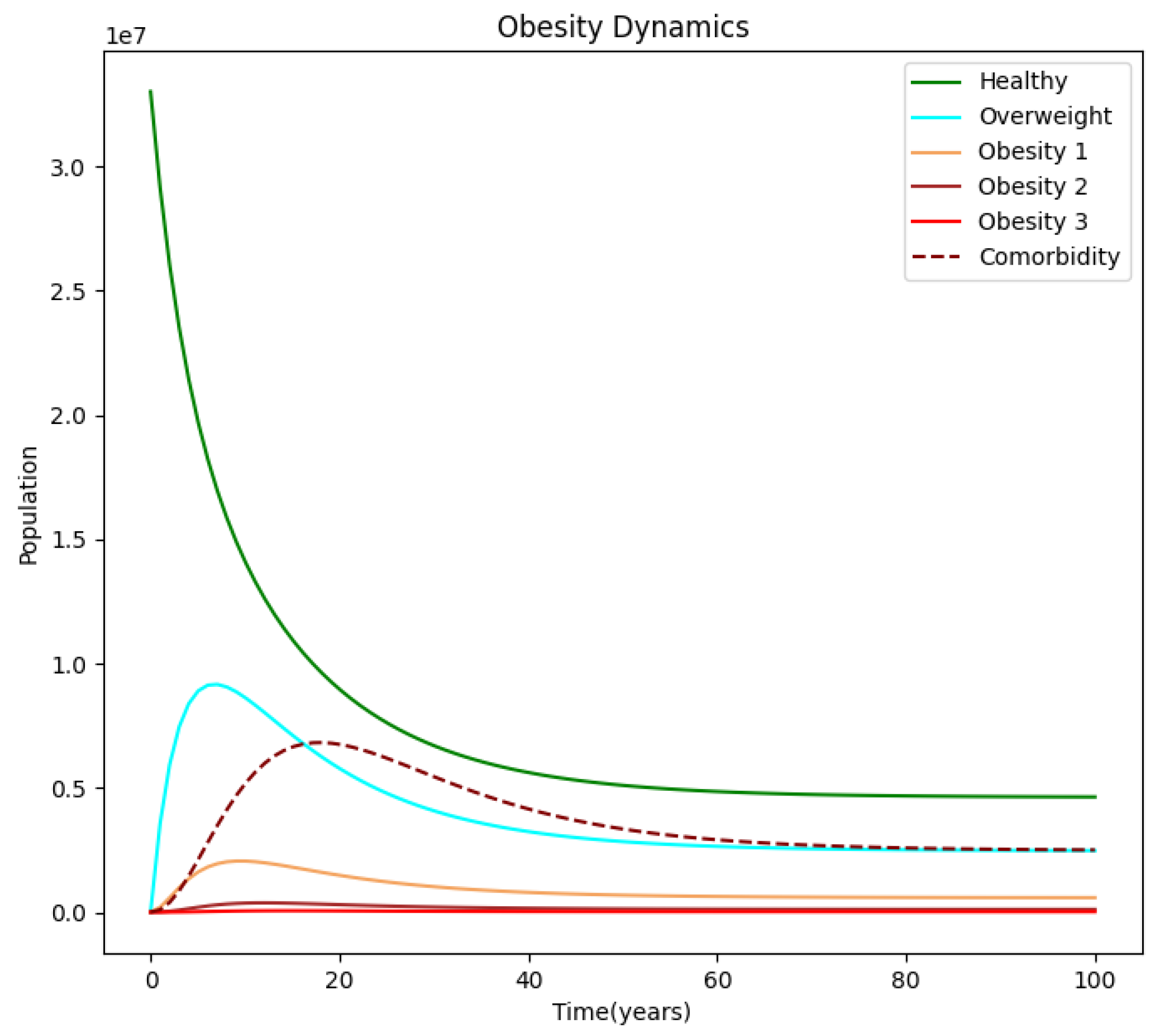
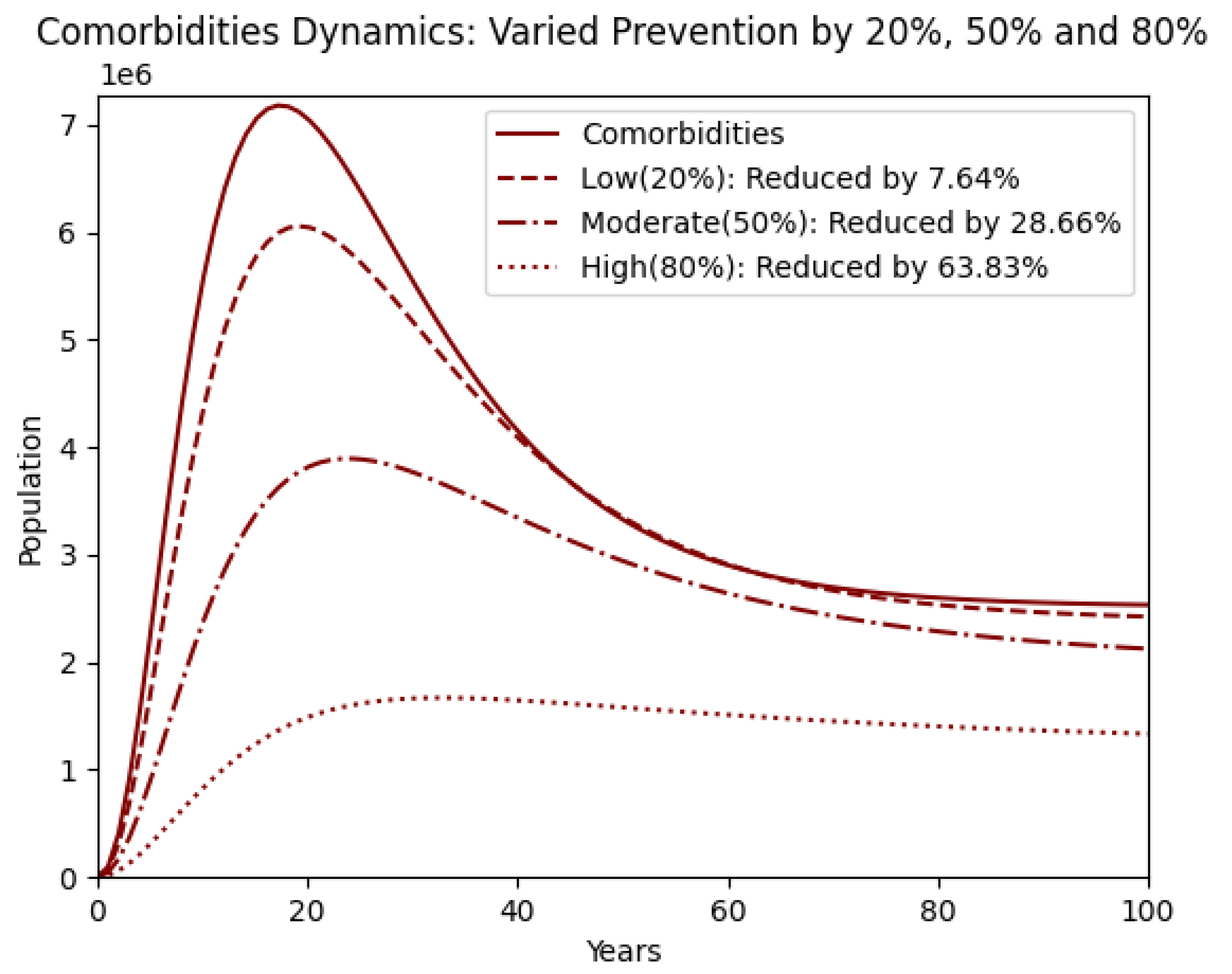
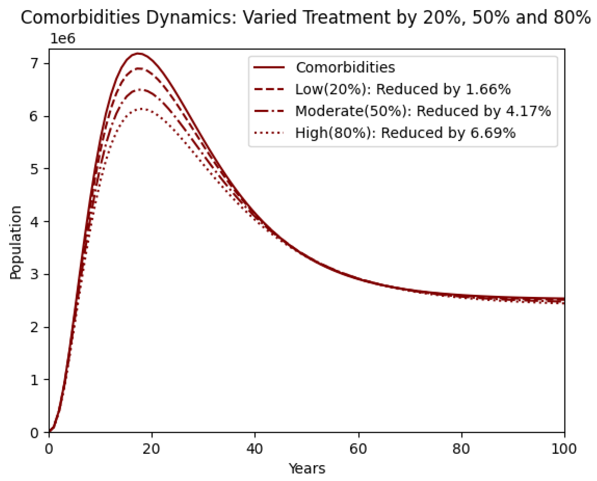
5. Numerical Results and Discussions

In this section, we present some numerical results and discussions for system (2) to illustrate the findings of the qualitative analysis of the model already conducted in the previous sections. To do this, we utilized the fourth-order Runge–Kutta method (RK4) and the Forward–Backward Sweeping method [34] in Python 3.11.0 with the SCIPY Library. The parameter values used in the simulations are provided in Table 3. These parameter values were sourced from previously published papers on the SA population, while others were estimated, as indicated in Table 3 and Remark 1. We assumed the initial conditions for the model to be $H\left(0\right)=33\times {10}^6$, representing the total number of healthy individuals in the population under study at the start of the simulation. All other compartments were initially set to zero: $V\left(0\right)=O_1\left(0\right)=O_2\left(0\right)=O_3\left(0\right)=C\left(0\right)=0$.

Figure 4 illustrates the overall dynamics of the six population compartments: healthy $H\left(t\right)$, overweight $V\left(t\right)$, class 1 obesity $O_1\left(t\right)$, class 2 obesity $O_2\left(t\right)$, class 3 obesity $O_3\left(t\right)$, and comorbidities $C\left(t\right)$. Over time, there was a gradual decline in the healthy and overweight populations, accompanied by a steady increase in all obesity classes and the comorbidity population. This trend reflects the natural progression of individuals from healthier weight categories into obesity and eventually comorbidity conditions in the absence of intervention, emphasizing the potential long-term public health burden.

Figure 5 explores the effect of varying levels of prevention strategies, modeled by reducing the transmission parameters $\beta =\{{\beta }_v,{\beta }_1,{\beta }_2,{\beta }_3\}$ by 20%, 50%, and 80% to represent low, moderate, and high prevention, respectively. The results show a substantial decrease in all obesity classes, with class 3 obesity exhibiting the highest sensitivity to increased prevention. The right-hand side of the figure aggregates the total obesity burden, clearly indicating that higher prevention efforts lead to proportionally greater reductions in the obese population.

Figure 6 presents the impact of the same prevention strategies on the comorbidity population. The downward trend becomes more pronounced with increasing levels of prevention, demonstrating a strong correlation between obesity reduction and the mitigation of related comorbidities. The graph highlights that high prevention (80%) leads to a substantial reduction in comorbidities of over 60%, showcasing the importance of upstream interventions to reduce the burden of chronic health conditions associated with obesity [10].

Figure 7 examines the effect of treatment strategies, represented by reductions in transition parameters $\tau =\{{\tau }_v,{\tau }_1,{\tau }_2,{\tau }_3\}$ by 20%, 50%, and 80%. The reduction in obesity classes is evident, though not as dramatic as with prevention. Higher treatment intensity yields better outcomes, particularly for class 2 and class 3 obesity. However, even at 80% treatment effort, the reductions are moderate, underscoring the limited effectiveness of treatment alone compared to preventive measures [35].

Figure 8 continues the analysis of treatment by focusing on the comorbidity population. The reductions here are also less pronounced than those seen with prevention. This suggests that treatment, while beneficial, may not sufficiently curb the development of obesity-related comorbidities unless combined with more robust preventive efforts. The graph shows that even high treatment levels only lead to modest decreases in comorbidity prevalence, reaffirming the need for integrated strategies [2].

Figure 9 illustrates the population dynamics of obesity classes and comorbidities over a 100-year period under different intervention levels. With increased prevention and treatment, the peak population decreases progressively, and the decline becomes more pronounced over time. This suggests that higher intervention rates significantly mitigate the prevalence of comorbidities, with the 80% intervention showing the most substantial reduction. These findings align with a study by the World Health Organization (WHO), which indicates that comprehensive prevention and treatment strategies can reduce the burden of comorbidities by up to 70% with high adherence rates [28,36].

Figure 10 compares two strategies, lifestyle modifications and the use of medications, on the obesity classes. Lifestyle changes produce more substantial reductions in all three obesity classes than medication alone. The figure on the right, which combines the obesity populations, further confirms the superior impact of lifestyle-based interventions. This suggests that promoting behavioral and dietary changes should be prioritized in obesity control policies [29].

Figure 11 examines the same strategies on the comorbidity population. Lifestyle modifications again outperform medications in reducing the number of individuals developing comorbidities. This emphasizes that while medications may assist in managing weight, their effect on long-term health outcomes is limited unless coupled with sustainable lifestyle changes [35].

Figure 12 presents a comparison of obesity class populations under a combined strategy, integrating both lifestyle modifications and medications against a no-control scenario. The combined approach yields the most substantial reduction across all obesity classes. The aggregate plot demonstrates the synergistic effect of combining interventions, indicating that a multi-pronged strategy is more effective than either approach alone [1].

Figure 13 extends this comparison to the comorbidity population. The combined strategy achieves a dramatic decline in comorbidities, significantly outperforming the uncontrolled case. This graph reinforces the idea that comprehensive obesity management targeting both behavioral and medical aspects is critical for reducing the broader public health burden of obesity-related diseases.

The influence of different prevention and treatment intensities on obesity classes and comorbidities is systematically summarized in

Table 5. Summary of effects of varying prevention and treatment parameters. $O=O_1+O_2+O_3$ is the sum of all obesity classes 1, 2, and 3. $O_1=$ obesity class 1, $O_2=$ obesity class 2, $O_3=$ obesity class 3 and $C=$ comorbidities.

Target	Varying	${\mathit{O}}_1$	${\mathit{O}}_2$	${\mathit{O}}_3$	O	C
Prevention	Low (20%)	7.78%	22.32%	37.88%	12.51%	7.64%
	Moderate (50%)	33.88%	74.32%	94.31%	45.5%	28.66%
	High (80%)	78.61%	96.55%	99.69%	83.39%	63.83%
Treatment	Low (20%)	1.71%	3.32%	5.51%	2.26%	1.66%
	Moderate (50%)	7.32%	8.18%	13.21%	5.64%	4.17%
	High (80%)	6.97%	12.89%	20.28%	8.97%	6.69%
Prevention + Treatment	Low (20%)	10.12%	25.68%	41.92%	15.16%	9.73%
	Moderate (50%)	39.31%	67.16%	84.51%	47.55%	53.46%
	High (80%)	83.36%	96.25%	99.32%	86.85%	71.83%

.

Remark 3.

Table 6. Optimal control graphs summary (%), with the percentage reductions each control strategy yields. $O_1=$ obesity class 1, $O_2=$ obesity class 2, $O_3=$ obesity class 3, $O_1+O_2+O_3=$ obesity classes, and $C=$ comorbidities.

Controls	${\mathit{O}}_1$	${\mathit{O}}_2$	${\mathit{O}}_2$	O	C
Lifestyle	$77.19\%$	$95.29\%$	$99.24\%$	$82.04\%$	$59.79\%$
Medication	$49.81\%$	$85.98\%$	$98.3\%$	$60.53\%$	$10.25\%$
Combining strategies	$92.16\%$	$99.48\%$	$99.97\%$	$94.06\%$	$65.97\%$

presents the following key insights that are critical for interpreting the impact of various intervention strategies:

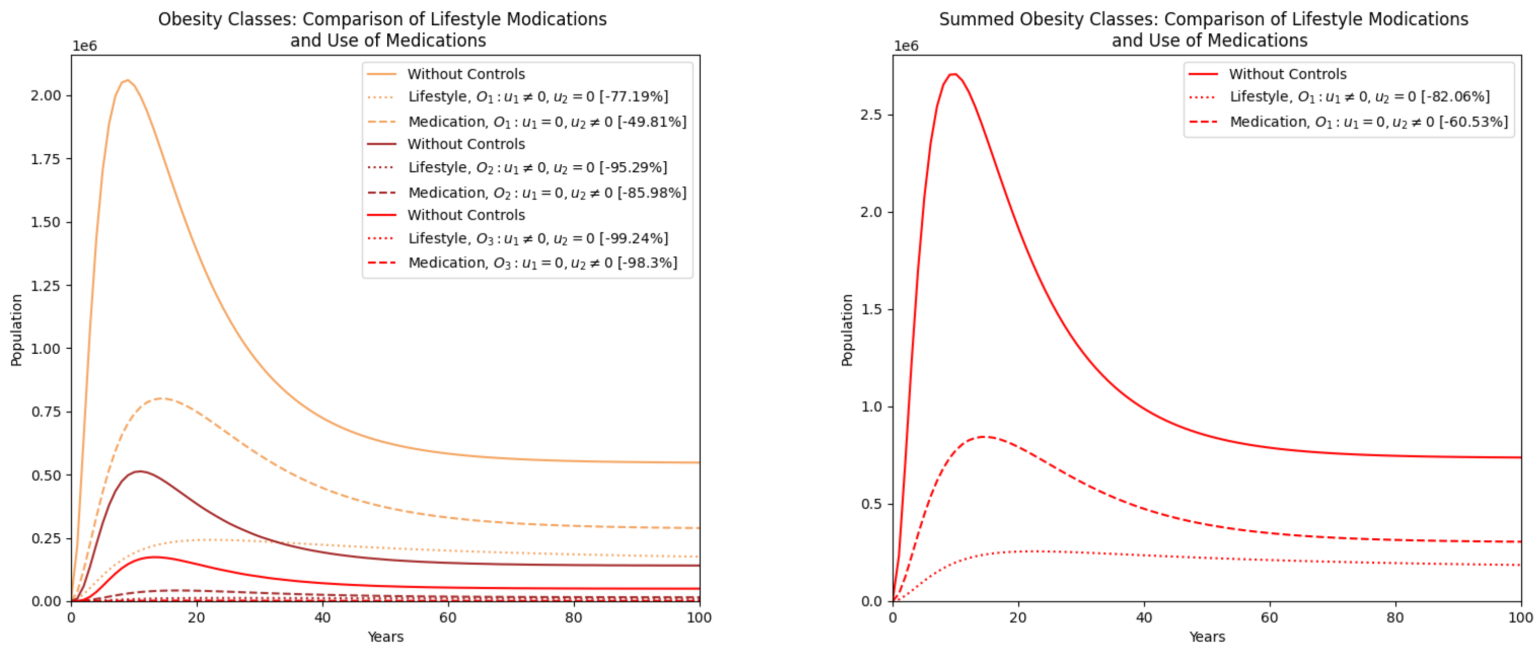
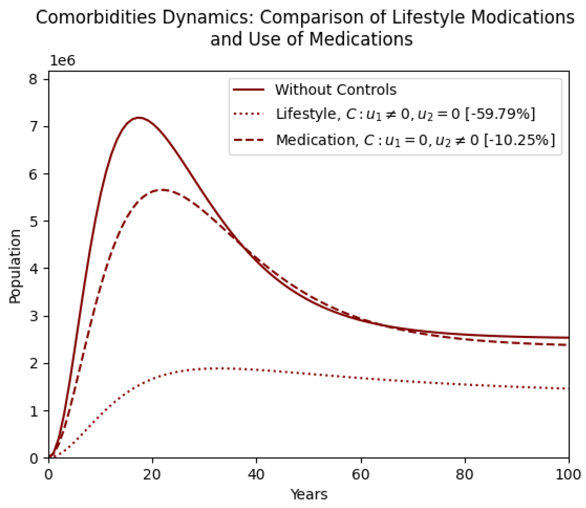
1. 

Lifestyle interventions independently produce the highest reductions in total obesity ($82.04\%$) and comorbidities ($59.79\%$), highlighting the effectiveness of prevention-based strategies.

2. 

Medication alone demonstrates moderate efficacy, particularly in mitigating higher obesity classes, but yields a limited impact on comorbidity reduction ($10.25\%$).

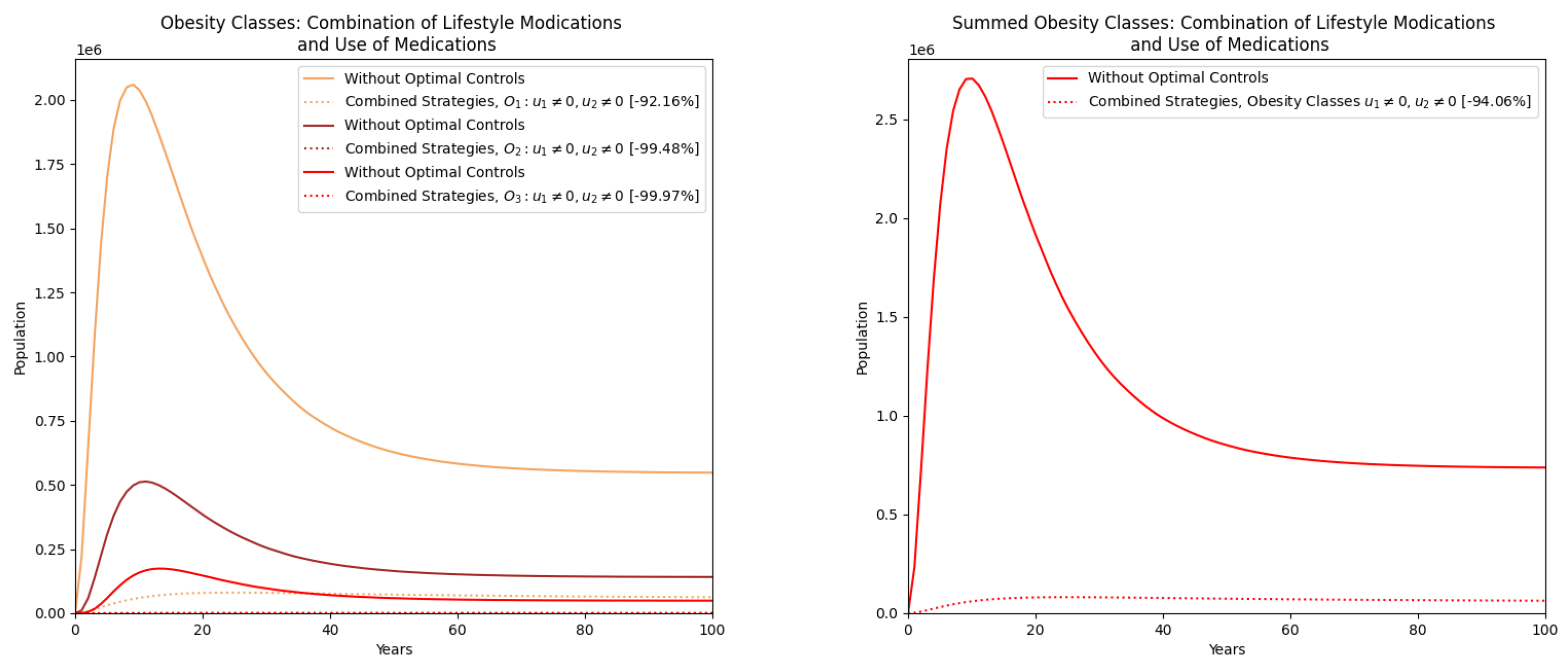
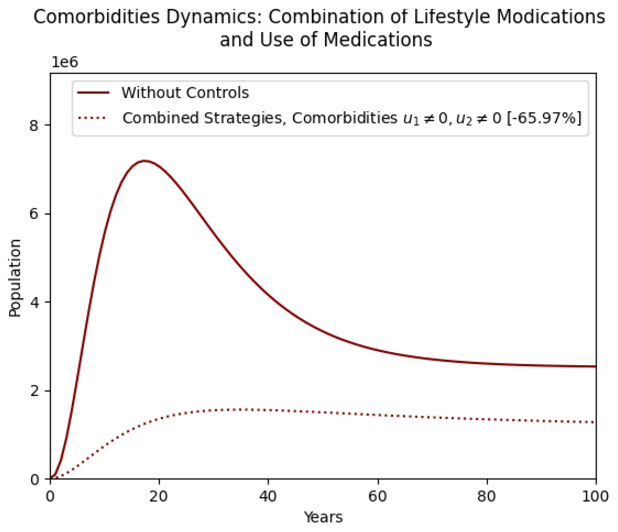
3. 

Combined strategies, incorporating both lifestyle modifications and medication, result in the most pronounced outcomes, reducing total obesity by $94.06\%$ and comorbidities by $65.97\%$.

4. 

Integrating lifestyle and medication interventions leads to greater reductions in obesity and comorbidities than single methods, highlighting the need for comprehensive, prevention-focused public health policies.

6. Conclusions

This study presented a novel mathematical model aimed at understanding and managing obesity along with its associated comorbidities. The framework was developed under mathematically sufficient conditions that ensured all solutions remained positive and bounded over time. The stability of the obesity-free equilibrium (OFE) was assessed using the Routh–Hurwitz criteria and Metzler matrix techniques, establishing both local and global stability. Optimal intervention strategies were formulated using the Pontryagin maximum principle (PMP), offering a structured approach to guide the system toward a healthier equilibrium state.

Numerical simulations were performed using the fourth-order Runge–Kutta method in combination with the Forward–Backward Sweeping algorithm. The results highlighted that prevention-oriented strategies, such as promoting healthier diets and increased physical activity, were significantly more effective in reducing obesity prevalence and its associated health burdens than treatment-based approaches.

Specifically, curative interventions were shown to reduce comorbidities by approximately 6%, whereas preventive measures could reduce them by up to 60%. If widely implemented, such strategies have the potential to lower obesity prevalence by around 80% and reduce comorbidities by a comparable margin. The most significant improvements were seen when combining preventive lifestyle changes with medical treatment, achieving over 90% reductions in both obesity and its related complications.

These results reinforce the conclusion that lifestyle-based interventions represent the most viable, impactful, and cost-effective solution for addressing long-term obesity concerns. As such, health authorities in Saudi Arabia are encouraged to prioritize these preventive measures within public health policy to realize sustainable improvements in population well-being.

Although this study calibrated the model using available demographic and obesity data from recent studies conducted in Saudi Arabia, the model is structurally flexible and can be adapted to other populations by adjusting the initial conditions and parameter values to reflect region-specific characteristics. This adaptability enables its application across various countries with differing demographic profiles and healthcare systems. Future studies should focus on calibrating and validating the model using recent and detailed data specific to the population under investigation, thereby enhancing its forecasting accuracy and relevance to regional health strategies.

References

- World Obesity Federation. World Obesity Atlas. 2023. Available online: https://data.worldobesity.org/publications/?cat=19 (accessed on 21 November 2024).
- World Health Organization. Obesity and Overweight. 1 March 2024. Available online: https://www.who.int/news-room/fact-sheets/detail/obesity-and-overweight (accessed on 21 November 2024).
- Alluhidan, M.; Alsukait, R.F.; Alghaith, T.; Shekar, M.; Alazemi, N.; Herbst, C.H. Overweight and Obesity in Saudi Arabia: Consequences and Solutions; World Bank: Washington, DC, USA, 2022. [Google Scholar] [CrossRef]
- Althumiri, N.A.; Basyouni, M.H.; AlMousa, N.; AlJuwaysim, M.F.; Almubark, R.A.; BinDhim, N.F.; Alkhamaali, Z.; Alqahtani, S.A. Obesity in Saudi Arabia in 2020: Prevalence, distribution, and its current association with various health conditions. Healthcare 2021, 9, 311. [Google Scholar] [CrossRef] [PubMed]
- Al-Raddadi, R.; Bahijri, S.M.; Jambi, H.A.; Ferns, G.; Tuomilehto, J. The prevalence of obesity and overweight, associated demographic and lifestyle factors, and health status in the adult population of Jeddah, Saudi Arabia. Ther. Adv. Chronic Dis. 2019, 10, 2040622319878997. [Google Scholar] [CrossRef]
- Al-Hazzaa, H.M.; Abahussain, N.A.; Al-Sobayel, H.I.; Qahwaji, D.M.; Musaiger, A.O. Physical activity, sedentary behaviors and dietary habits among Saudi adolescents relative to age, gender and region. Int. J. Behav. Nutr. Phys. Act. 2011, 8, 140. [Google Scholar] [CrossRef]
- Alsulami, S.; Baig, M.; Ahmad, T.; Althagafi, N.; Hazzazi, E.; Alsayed, R.; Alghamdi, M.; Almohammadi, T. Obesity prevalence, physical activity, and dietary practices among adults in Saudi Arabia. Front. Public Health 2023, 11, 1124051. [Google Scholar] [CrossRef]
- Jódar, L.; Santonja, F.J.; González-Parra, G. Modeling dynamics of infant obesity in the region of Valencia, Spain. Comput. Math. Appl. 2008, 56, 679–689. [Google Scholar] [CrossRef]
- Santonja, F.-J.; Villanueva, R.-J.; Jódar, L.; Gonzalez-Parra, G. Mathematical modelling of social obesity epidemic in the region of Valencia, Spain. Math. Comput. Model. Dyn. Syst. 2010, 16, 23–34. [Google Scholar] [CrossRef]
- Ejima, K.; Thomas, D.M.; Allison, D.B. A Mathematical Model for Predicting Obesity Transmission with Both Genetic and Nongenetic Heredity. Obesity 2018, 26, 927–933. [Google Scholar] [CrossRef]
- Al-Tuwairqi, S.M.; Matbouli, R.T. Modeling dynamics of fast food and obesity for evaluating the peer pressure effect and workout impact. Adv. Differ. Equ. 2021, 2021, 59. [Google Scholar] [CrossRef]
- Ku-Carrillo, R.A.; Delgadillo, S.E.; Chen-Charpentier, B.M. A mathematical model for the effect of obesity on cancer growth and on the immune system response. Appl. Math. Model. 2016, 40, 4908–4920. [Google Scholar] [CrossRef]
- Ku-Carrillo, R.A.; Delgadillo-Aleman, S.E.; Chen-Charpentier, B.M. Effects of the obesity on optimal control schedules of chemotherapy on a cancerous tumor. J. Comput. Appl. Math. 2017, 309, 603–610. [Google Scholar] [CrossRef]
- Siewe, N.; Friedman, A. A mathematical model of obesity-induced type 2 diabetes and efficacy of an anti-diabetic weight-reducing drug. J. Theor. Biol. 2024, 581, 111756. [Google Scholar] [CrossRef] [PubMed]
- Dehingia, K.; Yao, S.W.; Sadri, K.; Das, A.; Sarmah, H.K.; Zeb, A.; Inc, M. A study on cancer-obesity-treatment model with quadratic optimal control approach for better outcomes. Results Phys. 2022, 42, 105963. [Google Scholar] [CrossRef]
- Aldila, D.; Rarasati, N.; Nuraini, N.; Soewono, E. Optimal Control Problem of Treatment for Obesity in a Closed Population. Int. J. Math. Math. Sci. 2014, 2014, 273037. [Google Scholar] [CrossRef]
- Fatima, B.; Ikhlaq, M.; Zaman, G. The obesity prevention strategies in population dynamics. Adv. Model. Optim. 2017, 19, 213–225. [Google Scholar]
- Yanovski, S.Z.; Donato, K.; Gansheroff, L. The Obesity Epidemic: The Role of the National Institutes of Health. Adv. Stud. Med. 2005, 5, 122–123. [Google Scholar]
- Alshammari, F.S. A Mathematical Model to Investigate the Transmission of COVID-19 in the Kingdom of Saudi Arabia. Comput. Math. Methods Med. 2020, 2020, 9136157. [Google Scholar] [CrossRef]
- Moya, E.D.; Pietrus, A.; Bernard, S. A mathematical model for the study of obesity in a population and its impact on the growth of diabetes. Math. Model. Anal. 2023, 28, 611–635. [Google Scholar] [CrossRef]
- Guh, D.P.; Zhang, W.; Bansback, N.; Amarsi, Z.; Birmingham, C.L.; Anis, A.H. The incidence of co-morbidities related to obesity and overweight: A systematic review and meta-analysis. BMC Public Health 2009, 9, 88. [Google Scholar] [CrossRef]
- Apovian, C.M.; Aronne, L.J.; Barenbaum, S. Obesity Comorbidities: Clinical Guidance. Healio, 2024. Available online: https://www.healio.com/clinical-guidance/obesity/obesity-related-comorbidities (accessed on 29 November 2024).
- Lartey, S.T.; Si, L.; Otahal, P.; de Graaff, B.; Boateng, G.O.; Biritwum, R.B.; Minicuci, N.; Kowal, P.; Magnussen, C.G.; Palmer, A.J. Annual transition probabilities of overweight and obesity in older adults: Evidence from World Health Organization Study on global AGEing and adult health. Soc. Sci. Med. 2020, 247, 112821. [Google Scholar] [CrossRef]
- Ahmad, S.; Kirane, M. On a fractional-order mathematical model to assess the impact of diabetes and its associated complications in the United Arab Emirates. Math. Methods Appl. Sci. 2024, 47, 6892–6902. [Google Scholar] [CrossRef]
- Pearson-Stuttard, J.; Holloway, S.; Sommer Matthiessen, K.; Thompson, A.; Capucci, S. Variations in healthcare costs by body mass index and obesity-related complications in a UK population: A retrospective open cohort study. Diabetes Obes. Metab. 2024, 26, 5036–5045. [Google Scholar] [CrossRef] [PubMed]
- Hall, K.D.; Kahan, S. Maintenance of lost weight and long-term management of obesity. Med. Clin. N. Am. 2018, 102, 183–197. [Google Scholar] [CrossRef] [PubMed]
- Orwa, T.O.; Mbogo, R.W.; Luboobi, L.S. Multiple-Strain Malaria Infection and Its Impacts on Plasmodium falciparum Resistance to Antimalarial Therapy: A Mathematical Modelling Perspective. Comput. Math. Methods Med. 2019, 2019, 9783986. [Google Scholar] [CrossRef]
- Skou, S.T.; Mair, F.S.; Fortin, M.; Guthrie, B.; Nunes, B.P.; Miranda, J.J.; Boyd, C.M.; Pati, S.; Mtenga, S.; Smith, S.M. Multimorbidity. Nat. Rev. Dis. Primers 2022, 8, 48. [Google Scholar] [CrossRef]
- Van Baak, M.A.; Pramono, A.; Battista, F.; Beaulieu, K.; Blundell, J.E.; Busetto, L.; Carraça, E.V.; Dicker, D.; Encantado, J.; Ermolao, A.; et al. Effect of different types of regular exercise on physical fitness in adults with overweight or obesity: Systematic review and meta-analyses. Obesity Rev. 2021, 22, e13239. [Google Scholar] [CrossRef]
- Veit, M.; van Asten, R.; Olie, A.; Prinz, P. The role of dietary sugars, overweight, and obesity in type 2 diabetes mellitus: A narrative review. Eur. J. Clin. Nutr. 2022, 76, 1497–1501. [Google Scholar] [CrossRef]
- Ayele, T.K.; Goufo, E.F.D.; Mugisha, S. Mathematical modeling of HIV/AIDS with optimal control: A case study in Ethiopia. Results Phys. 2021, 26, 104263. [Google Scholar] [CrossRef]
- Cheneke, K.R. Optimal control and bifurcation analysis of HIV model. Comput. Math. Methods Med. 2023, 2023, 4754426. [Google Scholar] [CrossRef]
- Pontryagin, L.S. The Mathematical Theory of Optimal Processes; John Wilely & Sons: Hoboken, NJ, USA, 1962; Chapter 2. [Google Scholar]
- Lenhart, S.; Workman, J.T. Optimal Control Applied to Biological Models; Chapman and Hall/CRC: Boca Raton, FL, USA, 2007. [Google Scholar] [CrossRef]
- Ahmad, N.N.; Robinson, S.; Kennedy-Martin, T.; Poon, J.L.; Kan, H. Clinical outcomes associated with anti-obesity medications in real-world practice: A systematic literature review. Obes. Rev. 2021, 22, e13326. [Google Scholar] [CrossRef]
- May, A.L.; Freedman, D.; Sherry, B.; Blanck, H.M.; Centers for Disease Control and Prevention (CDC). Obesity United States, 1999–2010. MMWR Suppl. 2013, 62, 120–128. [Google Scholar] [PubMed]