Abstract
Polycystic Ovary Syndrome (PCOS) is a widespread hormonal disorder affecting women of reproductive age, often leading to infertility and associated complications. This study presents a comprehensive stochastic mathematical framework to analyze the dynamics of PCOS with a particular focus on infertility and treatment outcomes. Here, the transitions between compartments represent progression of women through clinical states of PCOS (risk, diagnosis, treatment, recovery) rather than infection or transmission, since PCOS is a non-communicable disorder. The model incorporates probabilistic elements to break the symmetric and predictable assumptions inherent in deterministic approaches. This allows it to reflect the randomness and asymmetry in hormonal regulation and ovulation cycles, enabling a more realistic representation of disease progression. By utilizing stochastic differential equations, the study evaluates the impact of treatment adherence on fertility restoration. We establish the conditions for disease extinction versus the existence of an ergodic stationary distribution, which represents a form of long-term statistical symmetry. The results emphasize the importance of early diagnosis and consistent treatment. Furthermore, the proposed approach provides a valuable tool for clinicians to predict patient-specific trajectories and optimize individualized treatment plans, accounting for the asymmetric nature of patient responses.
1. Introduction
Polycystic Ovary Syndrome (PCOS), also known as hyperandrogenic anovulation, is a prevalent endocrine disorder that significantly affects women’s reproductive health. The severity of complications associated with PCOS varies widely, ranging from mild metabolic disturbances to severe reproductive and systemic implications. Several factors contribute to the onset and progression of PCOS, including genetic predisposition, environmental influences, dietary habits, sedentary lifestyles, exposure to endocrine-disrupting chemicals, inflammatory processes, disruptions in steroid hormone synthesis and obesity.
At its core, PCOS arises from hormonal imbalances that disrupt normal reproductive functions, leading to the formation of ovarian cysts. According to Dennett and Simon [1], these fluid-filled sacs develop into functional cysts, which inhibit the regular release of oocytes necessary for fertilization. Consequently, this disruption results in menstrual irregularities such as amenorrhea and significantly impairs fertility. Clinically, PCOS is characterized by multiple ovarian cysts, typically ranging in size from 8 to 10 mm [2], which can obstruct normal ovulation and increase the risk of miscarriage.
Beyond infertility, PCOS is associated with several pregnancy-related complications, including gestational diabetes, pre-eclampsia, hypertension and preterm birth. The endocrine system plays a crucial role in maintaining reproductive health, with hormonal balance being regulated through the pulsatile secretion of hypothalamic gonadotropin-releasing hormone (GnRH), luteinizing hormone (LH) and follicle-stimulating hormone (FSH), as described by Tsutsumi and Webster [3]. Disruptions in this hormonal axis, often exacerbated by hyperprolactinemia and androgen excess, lead to impaired GnRH secretion [4] and an altered LH-to-FSH ratio, a hallmark of PCOS.
For a comprehensive understanding of PCOS and its broader implications, readers are encouraged to explore existing literature on the subject [5,6,7,8]. Building upon these foundational studies, Batool et al. [9] introduced a deterministic mathematical model for PCOS. Although the model uses a compartmental framework similar to infectious disease dynamics, the transitions represent incidence and progression rates rather than contagion. We adopt and extend this interpretation here by incorporating stochasticity.
The initial conditions are:
It is important to note that although the term has the algebraic form of a mass-action incidence, in this context it does not represent infection or transmission, since PCOS is a non-communicable condition. Instead, it denotes the incidence/progression rate at which susceptible women (S) develop PCOS (I), influenced by underlying risk factors such as obesity, insulin resistance, genetic predisposition and lifestyle. At any given time, women are classified into different groups based on their fertility status: those susceptible to infertility (denoted by ), individuals diagnosed with PCOS (), women undergoing infertility treatment with gonadotropins and clomiphene citrate () and those who have successfully overcome infertility ().
The parameter represents the frequency of patient visits to the clinic for diagnosis and treatment of the condition. Miscarriage and subsequent initiation of a new treatment cycle occur at a rate denoted by . The rate of therapy administration for women who have achieved pregnancy with medication (gonadotropins and clomiphene citrate) is represented by . The treatment rates in the patient class and the group receiving medical therapy are denoted by and , respectively. The recovery rate of group is . The number of recoveries in group is expressed as , where is the recovery rate of at time t. The influx of infertile women seeking treatment is represented by .
It is important to clarify that the appearance of treated individuals (T) in the interaction term does not imply direct physical interaction between susceptible and treated women. Since PCOS is not a transmissible disease, the term instead represents a .treatment-influenced progression rate: the dynamics of treatment cycles (such as recurrence after miscarriage, restarting therapy or discontinuation) affect the effective incidence of PCOS among susceptible women. Thus, the role of T is to capture how treatment pathways modify the flow of women through clinical states, rather than to indicate direct contagion. The success rates for subsequent IVF cycles, abortion rates and miscarriage rates are informed by clinical studies and expert consensus. For example, Kotlyar and Seifer (2023) provide a comprehensive review of therapeutic strategies for women with PCOS undergoing IVF, which emphasizes the complexities of achieving successful outcomes and highlights the need for personalized treatment plans to improve IVF success rates in these patients [10]. Additionally, Sun et al. (2020) conducted a systematic review and meta-analysis examining the risk factors for spontaneous abortion in patients with PCOS undergoing assisted reproductive treatment. Their findings suggest that high BMI and insulin resistance are significant risk factors for spontaneous abortion in this patient population [11]. Moreover, Mayrhofer et al. (2020) conducted a cohort study and meta-analysis on the prevalence and impact of PCOS in recurrent miscarriage. Their research confirms that women with PCOS experience higher rates of miscarriage compared to the general population [12].
From the dynamics of diseases, it is clear that real-world settings introduce inherent noise, therefore, it is essential to incorporate stochasticity into infectious disease models. To capture this randomness, stochastic calculus has emerged as a powerful approach. Several disease models have been analyzed using stochastic differential equations (SDEs) in the literature, including models for HBV [13,14], COVID-19 [15,16], HIV [17,18], influenza [19], childhood [20] and among others [21,22,23,24]. On the top of that, SDEs have been utilized in other fields of science such as mathematical physics [25,26,27,28], biological systems [29,30,31], fluid systems [32,33] and many more [34,35,36,37].
Model Assumptions and Justification for Stochastic Modeling
The model makes several key assumptions to simplify the complex biological and clinical processes involved in PCOS and treatment outcomes. These include:
Homogeneous patient population: The model assumes a general patient cohort with typical clinical characteristics of PCOS, though individual variation is accounted for through stochasticity.
Constant treatment protocols: Treatment options and success rates are assumed to be constant across time, though in practice, they may evolve with new therapies or medical advances.
Simplified disease progression: The disease progression of PCOS is modeled through a set of compartments with transitions between these states governed by stochastic processes. In particular, the transition should not be interpreted as infectious transmission. Rather, it captures the progression from being at risk (S) to developing PCOS (I) due to risk factors such as obesity, insulin resistance, genetic predisposition and lifestyle influences. We retain the compartmental notation for mathematical tractability, but stress that its interpretation is fundamentally different from epidemic contagion models.
In the context of PCOS, a stochastic model is preferred over a deterministic model because it allows for the representation of inherent variability and uncertainty. PCOS is influenced by multiple factors that are difficult to quantify deterministically, such as fluctuations in hormonal levels and individual responses to treatment. These factors lead to variability in clinical outcomes that a deterministic model cannot adequately capture.
A deterministic model would assume fixed, symmetric relationships between variables, which would not reflect the natural variation and asymmetry observed in clinical practice. In contrast, a stochastic model breaks this symmetry by introducing random variables, enabling more accurate predictions. This is especially important in PCOS, where treatment effectiveness varies widely among individuals. The stochastic approach allows for a more comprehensive understanding of the uncertainty surrounding disease progression and treatment efficacy, capturing the asymmetric paths patient outcomes can take.
Therefore, we utilize a stochastic approach to analyze the proposed PCOS model (1). The stochastic representation of this model is as follows:
In this model, we incorporate stochasticity through the use of stochastic differential equations (SDEs). The terms represent independent Brownian motions (white noises) associated with each compartment of the model () and is the intensity of the white noise. These stochastic terms introduce variability into the model, accounting for the random fluctuations in patient-specific factors such as treatment efficacy, hormonal imbalances and response to environmental factors. This randomness is particularly important in capturing the natural variability observed in the progression of PCOS and the impact of individual factors on treatment outcomes.
The rationale for using stochastic modeling is rooted in the inherently unpredictable nature of biological systems as discussed earlier as well. Factors such as the timing of ovulation, varying responses to medications and other patient-specific behaviors are difficult to predict deterministically, and hence, a stochastic approach is necessary to provide a more comprehensive and accurate representation of disease progression and fertility outcomes.
2. Mathematical Analysis of Model (2)
In this section, we perform a thorough analysis of the proposed stochastic model (2). We begin by examining the Markov process in , characterized by time-homogeneity and regularity. This process can be formally described by the following SDE:
Here, the dispersion matrix, commonly represented by , is typically defined as , here . The matrix here is utilized to construct the diffusion operator, often symbolized as . The definition of the diffusion operator is as follows:
When the operator acts on a function , the following takes place:
where
The above equations describe the stochastic behavior of the PCOS model in terms of its drift and diffusion components. The drift term, , represents the average or deterministic tendency of the system, capturing the biological processes such as recruitment, treatment, recovery and relapse among women undergoing therapy. The diffusion term, , models random fluctuations in these processes due to unpredictable biological or environmental factors, such as variations in treatment response or hormonal regulation. Hence, the diffusion operator mathematically characterizes how random effects influence the overall evolution of the PCOS population system over time.
Existence and Uniqueness of Solution
We now address the existence, uniqueness and positivity of the solution for model (2). Throughout this work, Lyapunov functions are used in the sense of stochastic stability theory [38,39]. Specifically, a function is called a Lyapunov function if it is positive definite, i.e., for all x with equality only at the equilibrium point, and its generator is negative definite (or non-positive), ensuring stability. In the proofs below, the functions and are constructed to satisfy these conditions and the analysis follows the standard framework in stochastic stability theory.
Theorem 1.
For any initial value , there exists a non-negative solution of the stochastic model (2) over , such that the solution remains within with a probability 1.
Proof.
Since the coefficients in system (2) satisfy the local Lipschitz condition, there exists a unique local solution for , where is the explosion time.
To prove global existence (), consider the Lyapunov function
Since for , we have .
Applying Itô’s formula to Y, we obtain
where and are the diffusion coefficients. The drift part satisfies
for some constant depending on the parameters and noise intensities.
Thus, is bounded in expectation for all , which rules out finite-time explosion. Therefore, and the solution remains in for all . □
3. Extinction of the Model
In this section, we analyze the conditions that lead to either the extinction of the disease or its persistence within the population. These two outcomes represent a fundamental symmetry breaking in the system’s dynamics. The disease-free state is a trivial equilibrium, a symmetric state where the infected population is zero. The persistence of the disease leads to an endemic equilibrium, which, in a stochastic context, manifests as a stationary distribution. This distribution represents a form of long-term statistical symmetry, where despite continuous random fluctuations, the overall system properties remain stable on average. We begin with the following definition:
The threshold quantity for the stochastic system (2) can be obtained as:
Lemma 1.
Suppose represents the solution of the considered model (2) with initial values , then
Moreover, if , then
This lemma is proved in [40], so some one can see the proof.
We verify that the subsequent theorem is valid by using our proposed model.
Theorem 2.
Assume denotes the solution of considered model (2) with initial values . Moreover, if and , then
If the disease diminishes exponentially and converges to 0, then will approach zero with probability one, indicating the eradication of the disease. Furthermore,
Proof.
We define the Lyapunov function , which is positive definite for . The infinitesimal generator of V is
Through the process of integration applied to model (2), we derive
To compute the basic reproductive number , we apply the next-generation matrix approach.
From model (1):
The disease-free equilibrium (DFE) occurs when and .
Following the next generation matrix method, we identify the infected compartments as and . Let the vector of infected states be .
The system describing the infected classes is:
where:
At the DFE (, ), the Jacobian matrices of and with respect to are:
The next generation matrix is:
Computing gives
Hence,
The dominant eigenvalue (spectral radius) of K is
Thus,
Furthermore, upon integrating the third equation of model (2) from 0 to t and subsequently dividing the resultant equation by t, we acquire
using Equation (15) and , we get
From first equation in model (12), we obtain
Lemma 2.
The Markov processes will have a unique ergodic stationary distribution whenever there exists a bounded open domain having boundary of regular type with characteristics:
(a) For every , the matrix must be positive definite.
(b) For , has a finite average duration, representing the time required from to reach and for all compact subsets . Then,
Here, the function shows the integrability of f with respect to π.
For the proof of this lemma see [40].
Theorem 3.
If (respectively, ), then the noise-modified production terms dominate (respectively, are dominated by) the removal terms in the sense made precise below. In particular, when the assumptions of Lemma 2 hold and the constants are chosen as in the proof, the process generated by (2) admits a unique stationary distribution and is ergodic.
Proof.
By Theorem 1 (existence and uniqueness) system (2) admits a unique global positive solution for any positive initial data. To prove the existence of a unique stationary distribution and ergodicity, we verify conditions (a) and (b) of Lemma 2 (non-degeneracy of diffusion and the existence of a suitable Lyapunov function whose generator is negative outside a compact set).
- (a)
- Non-degeneracy of the diffusion matrix.
The diffusion (covariance) matrix of (2) is diagonal with entries proportional to the squares of the state variables:
For any nonzero vector , we have
where Thus, the diffusion coefficient matrix is positive semi-definite and non-degenerate on any domain that excludes the coordinate axes; condition (a) of Lemma 2 is satisfied for domains away from the boundary. To handle the boundary, one uses standard boundary regularity arguments (this is the same reasoning used in [38]); we therefore proceed to construct a Lyapunov function for condition (b).
- (b)
- Lyapunov function and negativity of generator outside a compact set.
Define, for constants to be chosen later, the twice continuously differentiable function
This function tends to as any state variable tends to or any of tends to ; hence sublevel sets of are compact in .
Compute the infinitesimal generator of the diffusion process (apply Itô’s formula and collect drift and Itô correction terms). After straightforward algebra (omitted here for brevity) one obtains the estimate
where collects the remaining terms that are either bounded on compact sets or negative and of order at least linear in . The key point is that the negative cubic-root terms in the bracket dominate for large arguments.
Choose the constants to balance the positive and negative terms: a convenient choice is
With this choice, the leading negative term in (23) can be combined and bounded below by a cubic-root expression involving . In particular, after substitution and simplification there exists a positive constant (depending only on parameters and noise intensities) such that
where is bounded on compact sets and satisfies as after factoring the dominant negative term. Thus, if the leading term in (25) is strictly negative and dominates outside a sufficiently large compact set; equivalently, there exists a compact set and constants such that
and is bounded on K.
To make the negativity uniform and to obtain a coercive Lyapunov, define the modified function
with chosen large enough so that is positive and coercive. Set
so that and at the initial state. Computing and using (26) yields
for some compact set and . Thus, condition (b) of Lemma 2 is satisfied. By Lemma 2, since conditions (a) and (b) are satisfied, the Markov process defined by (2) admits a unique stationary distribution and is ergodic. This completes the proof. □
4. Numerical Demonstrations and Discussion
This section presents graphical representations accompanied by an analysis of the findings. The time is set to 20, with a step size of . Additionally, the initial values were set as . Furthermore, the values of the parameters considered for the simulation are presented in Table 1 taken from [9].

Table 1.
Descriptions, numerical values, and sources of parameters in model (2). Parameters which are not available in the literature are assumed in this study.
In Figure 1, the stochastic and deterministic dynamics of various state variables of the model (2) are visualized. Figure 2a shows the dynamics of the susceptible women, and Figure 2b demonstrates the behavior of infected women. It can be observed that there is an increase at the beginning of the simulations, resulting in a significant wave, followed by a decrease in their number. Similarly, the infections are seen to increase with time, as shown in Figure 2b. Furthermore, Figure 3a,b aim to present the dynamics in both stochastic and deterministic senses of the women under treatment and those who have recovered from the disease. In this observation, it is evident that the count within the treatment group decreases rapidly, followed by an increase in the number of patients receiving treatment. The number of recovered individuals decreases over time.
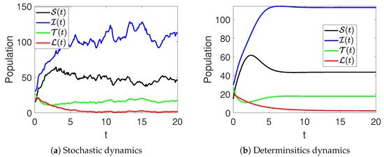
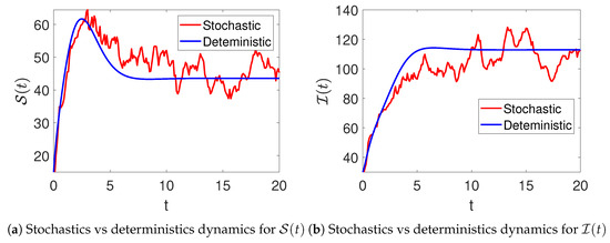
Figure 2.
Stochastic (red color) and deterministic (blue color) evolution of susceptible (a) and infected (b) women in model (2).
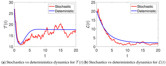
Figure 3.
The stochastic (red color) and the deterministic (blue color) evolution of under treatment (a) and recovered (b) women in model (2).
Parameters’ Effects on the Dynamics
This part of the manuscript aims to present the effects of various important parameters on the dynamics of infections and recovery. Figure 4 demonstrates the effects of the rate of abortion and restarting treatment () on the number of infections and recoveries among women. From the figure, it can be observed that when is increased, it leads to a decrease in the prevalence or severity of the polycystic virus. This is because elevated rates of abortion and treatment reinitiation expedite the eradication of the virus from infected women, thereby diminishing transmission and alleviating the overall disease burden across the population.
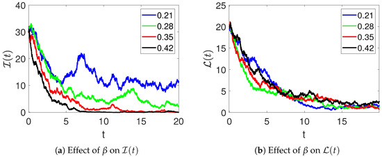
Figure 4.
The effects of the rate of abortion and restarting treatment on the number of infections (a) and recovery (b) of women in model (2).
Furthermore, the effects of the parameter on the dynamics of and are demonstrated in Figure 5. Here, it can be observed that the number of infections decreases, and the number of recoveries increases as the rate of treatment is increased. Figure 6 shows the effects of medical therapy () on infected and recovered individuals. The infected women recover faster as increases. Likewise, an increase in the number of women who recover is observed as more of them receive medical therapy.
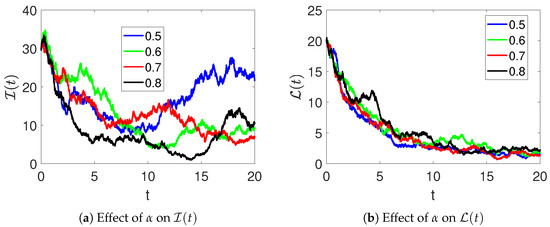
Figure 5.
The effects of the treatment rate on infected (a) and recovered (b) individuals in model (2).
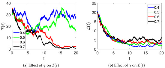
Figure 6.
The effects of the medical therapy on infected (a) and recovered (b) individuals in model (2).
An increase in (therapy rate) accelerates recovery, reducing the infected population over time, whereas smaller or values lead to slower recovery and higher disease persistence. This demonstrates the sensitivity of the system to treatment-related parameters.
The histograms in Figure 7 highlight the stochastic variability in population levels across repeated simulations. Each distribution is approximately unimodal, suggesting that despite random perturbations, the system tends to fluctuate around a stable mean for each compartment. The relatively narrow spread of , and indicates lower variance compared to , which shows higher dispersion due to stronger sensitivity to infection-related noise. These results quantitatively confirm the system’s tendency toward a stable stochastic equilibrium.
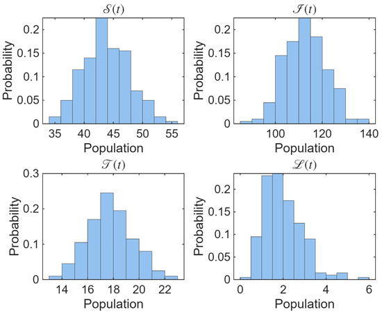
Figure 7.
The histograms portraying the distribution of population levels from multiple stochastic simulations of the proposed model.
Figure 8 displays the corresponding heatmaps showing the spatio-temporal evolution of population levels across multiple simulation runs. Each pixel encodes the population level at a specific time and simulation index, with the color intensity indicating the magnitude of the population density. The heatmaps reveal the temporal stability and random fluctuations of the system, illustrating how each compartment evolves under the influence of stochastic effects. Together, these plots provide a comprehensive visualization of variability and the long-term statistical stability of the model.
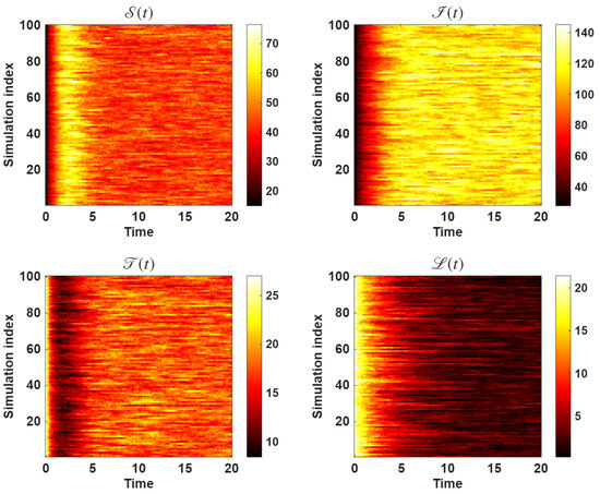
Figure 8.
The heatmap portraying the spatio-temporal evolution of population levels from multiple dynamics across multiple simulations of the proposed model.
In addition to the qualitative variability shown in the heatmaps, we computed the sample mean and variance of the system states based on 100 independent stochastic realizations. The variance was calculated as
where is the k-th realization and is the sample mean. The steady-state results are summarized in Table 2.
Table 2.
Sample mean and variance of each state variable based on 100 stochastic realizations at steady state.
Figure 9 illustrates the temporal evolution of the stochastic variance for the four compartments of the model. The variance of (patients undergoing treatment) is notably higher than that of the other compartments, indicating that the infected population is the most sensitive to random fluctuations in treatment and recovery dynamics. In contrast, and exhibit relatively low variance, suggesting that the susceptible and recovered classes remain more stable over time. These results align with the biological expectation that variability in treatment response and hormonal regulation primarily affects women under therapy rather than those in the recovered or susceptible states. Overall, the system tends toward a steady stochastic equilibrium, confirming the boundedness of random fluctuations around the mean trajectories.
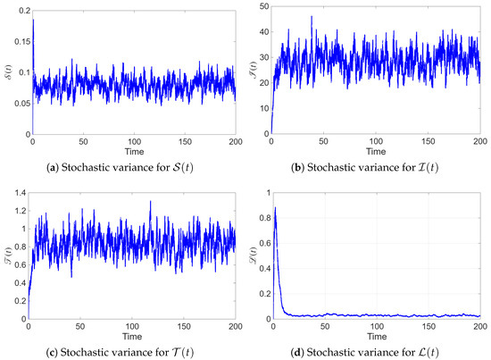
Figure 9.
Temporal evolution of the stochastic variance for each state variable in model (2).
The clinical relevance of the model extends beyond theoretical predictions and into practical applications for PCOS treatment. By incorporating stochasticity, the model allows for the simulation of various treatment scenarios under different patient conditions, thus enabling the optimization of treatment plans. For instance, the model can be used to simulate how different treatments (e.g., hormonal therapy, metformin or lifestyle interventions) affect the likelihood of ovulation, pregnancy and infertility over time. This can guide healthcare providers in tailoring treatment options based on the variability in patient responses, helping to optimize individual treatment plans.
Moreover, the model provide insights into the probability of infertility in different patient cohorts, based on their disease progression and treatment history. By considering the stochastic nature of the disease and its treatment, clinicians can use the model to predict the risk of infertility under various intervention strategies. This is particularly important in the management of PCOS, where the effectiveness of treatment can vary widely between individuals.
5. Conclusions
This article has analyzed a stochastic model for Polycystic Ovary Syndrome (PCOS) utilizing stochastic differential equations (SDEs). The study population was divided into four groups: women at risk for infertility, PCOS sufferers, infertile women undergoing therapy (gonadotropin and clomiphene citrate) and those showing improvement in infertility. Utilizing the Lyapunov method, we ensured the existence and uniqueness of a global positive solution. Moreover, we introduced two innovative thresholds to deduce the essential criteria for extinction and the ergodic stationary distribution (ESD). The Euler–Maruyama numerical procedure was implemented to perform numerical simulations of the considered model with and without Brownian motion. The numerical simulations validated the ESD and provided a comparative analysis of the model with and without noise. The effect of abortion, restarting treatment and medical therapy on the behavior of the infected and recovered populations was illustrated via numerical simulations.
From the simulations, we conclude that individuals diagnosed with PCOS should initially prioritize adhering to a nutritious eating plan. Healthcare professionals ought to devise tailored dietary plans, considering factors such as macronutrient proportions, micronutrient intake and overall calorie restriction, after conducting a thorough assessment of the patient’s previous dietary habits. Next, engaging in regular exercise proves beneficial for PCOS patients, aiding in weight management and altering body composition. Customized workout routines should be developed, considering factors such as muscle gain and fat loss, tailored to each patient’s unique muscle-to-fat ratio. Unlike infectious disease models, our framework does not imply transmission of PCOS between individuals. Instead, the compartmental flows reflect the stochastic progression and treatment dynamics of a non-communicable disorder.
Limitations and Future Research Directions
While the model provides valuable insights into treatment outcomes for women with PCOS, there are several limitations that need to be addressed in future work. One of the primary limitations of the current model is the assumption of a homogeneous patient population. In reality, PCOS is a heterogeneous condition, with substantial variability in disease severity, comorbidities and responses to treatment. In our model, all individuals are treated as having similar characteristics, including treatment protocols, success rates and responses to interventions. To address this limitation, future research could incorporate patient subgroups based on factors such as age, body mass index, insulin resistance and the severity of PCOS. This would allow for a more personalized approach to modeling treatment outcomes. Additionally, other sources of variability, such as environmental factors, genetic predispositions and lifestyle factors, could be incorporated into the model to improve its accuracy and realism.
Furthermore, the model assumes fixed transition probabilities between health states, which may not fully capture the complexities of disease progression and treatment outcomes in real-world settings. Future work could explore dynamic treatment protocols, where treatment success rates vary depending on patient characteristics, or incorporate more detailed data on treatment efficacy. Moreover, the comparisons of this work will include clinical outcomes such as ovulation rates, pregnancy success rates and the incidence of infertility. We recognize that the validation of the model with real-world data will be worth considering for establishing its clinical applicability. If such data are not readily accessible, the methods can be potentially validated, such as using longitudinal cohort studies, patient-specific treatment outcome data or clinical trial data to further calibrate and validate the model. By relaxing some of these assumptions, the model could be adapted to better reflect clinical practice, where treatment decisions are often made based on individual patient profiles.
These advancements would help improve the predictive power of the model and enhance its clinical relevance for guiding treatment strategies in women with PCOS.
The proposed model adopts a mass-action incidence term, consistent with previous PCOS modeling studies [6,9]. While this facilitates comparison across studies, a natural extension would be to reformulate the model using standard incidence , which is often considered more realistic for human populations. We anticipate that this modification would not change the qualitative stochastic results (extinction vs. persistence), but it would refine the biological interpretation of the incidence mechanism.
Author Contributions
Conceptualization, A.M.A.E.-l.; Formal analysis, M.A., B.M., A.M.A.E.-l. and S.O.A.; Investigation, A.E.; Methodology, K.A., A.A.Q., M.A., A.E. and S.O.A.; Project administration, K.A. and A.A.Q.; Software, B.M.; Supervision, K.A.; Writing—original draft, K.A., M.A., B.M. and A.E.; Writing—review & editing, A.A.Q., A.M.A.E.-l. and S.O.A. All authors have read and agreed to the published version of the manuscript.
Funding
This work was supported and funded by the Deanship of Scientific Research at Imam Mohammad Ibn Saud Islamic University (IMSIU) (grant number IMSIU-DDRSP2501).
Data Availability Statement
The original contributions presented in this study are included in the article. Further inquiries can be directed to the corresponding authors.
Conflicts of Interest
The authors declare no conflicts of interest.
References
- Dennett, C.C.; Simon, J. The role of polycystic ovary syndrome in reproductive and metabolic health: Overview and approaches for treatment. Diabetes Spectr. 2015, 28, 116–120. [Google Scholar] [CrossRef]
- Rausch, M.E.; Legro, R.S.; Barnhart, H.X.; Schlaff, W.D.; Carr, B.R.; Diamond, M.P.; Carson, S.A.; Steinkampf, M.P.; McGovern, P.G.; Cataldo, N.A.; et al. Predictors of pregnancy in women with polycystic ovary syndrome. J. Clin. Endocrinol. Metab. 2009, 94, 3458–3466. [Google Scholar] [CrossRef] [PubMed]
- Tsutsumi, R.; Webster, N.J.G. GnRH pulsatility, the pituitary response and reproductive dysfunction. Endocr. J. 2009, 56, 729–737. [Google Scholar] [CrossRef] [PubMed]
- Grattan, D.R.; Jasoni, C.L.; Liu, X.; Anderson, G.M.; Herbison, A.E. Prolactin regulation of gonadotropin-releasing hormone neurons to suppress luteinizing hormone secretion in mice. Endocrinology 2007, 148, 4344–4351. [Google Scholar] [CrossRef] [PubMed]
- Chaudhuri, A. Polycystic ovary syndrome: Causes, symptoms, pathophysiology, and remedies. Obes. Med. 2023, 39, 100480. [Google Scholar] [CrossRef]
- Hafezi, S.G.; Zand, M.A.; Molaei, M.; Eftekhar, M. Dynamic model with factors of polycystic ovarian syndrome in infertile women. Int. J. Reprod. Biomed. 2019, 17, 231. [Google Scholar]
- Tiwari, S.; Kane, L.; Koundal, D.; Jain, A.; Alhudhaif, A.; Polat, K.; Zaguia, A.; Alenezi, F.; Althubiti, S.A. SPOSDS: A smart Polycystic Ovary Syndrome diagnostic system using machine learning. Expert Syst. Appl. 2022, 203, 117592. [Google Scholar] [CrossRef]
- Nasim, S.; Almutairi, M.S.; Munir, K.; Raza, A.; Younas, F. A novel approach for polycystic ovary syndrome prediction using machine learning in bioinformatics. IEEE Access 2022, 10, 97610–97624. [Google Scholar] [CrossRef]
- Batool, M.; Farman, M.; Ahmad, A.; Nisar, K.S. Mathematical study of polycystic ovarian syndrome disease including medication treatment mechanism for infertility in women. AIMS Public Health 2023, 11, 19. [Google Scholar] [CrossRef]
- Kotlyar, A.M.; Seifer, D.B. Women with PCOS who undergo IVF: A comprehensive review of therapeutic strategies for successful outcomes. Reprod. Biol. Endocrinol. 2023, 21, 70. [Google Scholar] [CrossRef]
- Sun, Y.-F.; Zhang, J.; Xu, Y.-M.; Cao, Z.-Y.; Wang, Y.-Z.; Hao, G.-M.; Gao, B.-L. High BMI and insulin resistance are risk factors for spontaneous abortion in patients with polycystic ovary syndrome undergoing assisted reproductive treatment: A systematic review and meta-analysis. Front. Endocrinol. 2020, 11, 592495. [Google Scholar] [CrossRef]
- Mayrhofer, D.; Hager, M.; Walch, K.; Ghobrial, S.; Rogenhofer, N.; Marculescu, R.; Seemann, R.; Ott, J. The prevalence and impact of polycystic ovary syndrome in recurrent miscarriage: A retrospective cohort study and meta-analysis. J. Clin. Med. 2020, 9, 2700. [Google Scholar] [CrossRef] [PubMed]
- Din, A. Bifurcation analysis of a delayed stochastic HBV epidemic model: Cell-to-cell transmission. Chaos Solitons Fractals 2024, 181, 114714. [Google Scholar] [CrossRef]
- Din, A.; Sabbar, Y.; Wu, P. A novel stochastic Hepatitis B virus epidemic model with second-order multiplicative α-stable noise and real data. Acta Math. Sci. 2024, 44, 752–788. [Google Scholar] [CrossRef]
- Xu, C.; Pang, Y.; Liu, Z.; Shen, J.; Liao, M.; Li, P. Insights into COVID-19 stochastic modelling with effects of various transmission rates: Simulations with real statistical data from UK, Australia, Spain, and India. Phys. Scr. 2024, 99, 025218. [Google Scholar] [CrossRef]
- Mamis, K.; Farazmand, M. Stochastic compartmental models of the COVID-19 pandemic must have temporally correlated uncertainties. Proc. R. Soc. A 2023, 479, 20220568. [Google Scholar] [CrossRef]
- Lu, C.; Sun, G.; Zhang, Y. Stationary distribution and extinction of a multi-stage HIV model with nonlinear stochastic perturbation. J. Appl. Math. Comput. 2022, 68, 885–907. [Google Scholar] [CrossRef]
- Rao, F.; Tan, Y.; Lian, X. Stochastic analysis of an HIV model with various infection stages. Adv. Contin. Discret. Models 2025, 2025, 38. [Google Scholar] [CrossRef]
- Alzabut, J.; Alobaidi, G.; Hussain, S.; Madi, E.N.; Khan, H. Stochastic dynamics of influenza infection: Qualitative analysis and numerical results. Math. Biosci. Eng. 2022, 19, 10316–10331. [Google Scholar] [CrossRef]
- ur Rahman, G.; Badshah, Q.; Agarwal, R.P.; Islam, S. Ergodicity & dynamical aspects of a stochastic childhood disease model. Math. Comput. Simul. 2021, 182, 738–764. [Google Scholar] [CrossRef]
- Martheswaran, T.K.; Hamdi, H.; Al-Barty, A.; Zaid, A.A.; Das, B. Prediction of dengue fever outbreaks using climate variability and Markov chain Monte Carlo techniques in a stochastic susceptible-infected-removed model. Sci. Rep. 2022, 12, 5459. [Google Scholar] [CrossRef]
- Hajri, Y.; Assiri, T.A.; Amine, S.; Ahmad, S.; la Sen, M.D. A stochastic co-infection model for HIV-1 and HIV-2 epidemic incorporating drug resistance and dual saturated incidence rates. Alex. Eng. J. 2023, 84, 24–36. [Google Scholar] [CrossRef]
- Farah, E.M.; Amine, S.; Ahmad, S.; Nonlaopon, K.; Allali, K. Theoretical and numerical results of a stochastic model describing resistance and non-resistance strains of influenza. Eur. Phys. J. Plus 2022, 137, 1–15. [Google Scholar] [CrossRef]
- Ko, Y.; Mendoza, V.M.; Mendoza, R.; Seo, Y.; Lee, J.; Jung, E. Estimation of monkeypox spread in a nonendemic country considering contact tracing and self-reporting: A stochastic modeling study. J. Med. Virol. 2023, 95, e28232. [Google Scholar] [CrossRef]
- Alqahtani, A.M.; Akram, S.; Ahmad, J.; Aldwoah, K.A.; Rahman, M.u. Stochastic wave solutions of fractional Radhakrishnan–Kundu–Lakshmanan equation arising in optical fibers with their sensitivity analysis. J. Opt. 2024. In press. [Google Scholar] [CrossRef]
- Aldwoah, K.; Mustafa, A.; Aljaaidi, T.; Mohamed, K.; Alsulami, A.; Hassan, M. Exploring the impact of Brownian motion on novel closed-form solutions of the extended Kairat-II equation. PLoS ONE 2025, 20, e0314849. [Google Scholar] [CrossRef] [PubMed]
- Kamel, A.; Louati, H.Y.; Aldwoah, K.; Alqarni, F.; Almalahi, M.; Hleili, M. Stochastic analysis and soliton solutions of the Chaffee–Infante equation in nonlinear optical media. Bound. Value Probl. 2024, 2024, 119. [Google Scholar] [CrossRef]
- Baber, M.Z.; Ahmed, N.; Xu, C.; Iqbal, M.S.; Sulaiman, T.A. A computational scheme and its comparison with optical soliton solutions for the stochastic Chen–Lee–Liu equation with sensitivity analysis. Mod. Phys. Lett. B 2025, 39, 2450376. [Google Scholar] [CrossRef]
- Baber, M.Z.; Yasin, M.W.; Xu, C.; Ahmed, N.; Iqbal, M.S. Numerical and analytical study for the stochastic spatial dependent prey–predator dynamical system. J. Comput. Nonlinear Dyn. 2024, 19, 101003. [Google Scholar] [CrossRef]
- Zhang, S.; Zhang, T.; Yuan, S. Dynamics of a stochastic predator-prey model with habitat complexity and prey aggregation. Ecol. Complex. 2021, 45, 100889. [Google Scholar] [CrossRef]
- Lei, J.; Mackey, M.C. Stochastic differential delay equation, moment stability, and application to hematopoietic stem cell regulation system. SIAM J. Appl. Math. 2007, 67, 387–407. [Google Scholar] [CrossRef]
- Atzberger, P.J. Stochastic Eulerian Lagrangian methods for fluid–structure interactions with thermal fluctuations. J. Comput. Phys. 2011, 230, 2821–2837. [Google Scholar] [CrossRef]
- Bean, N.G.; O’Reilly, M.M. The stochastic fluid–fluid model: A stochastic fluid model driven by an uncountable-state process, which is a stochastic fluid model itself. Stoch. Processes Their Appl. 2014, 124, 1741–1772. [Google Scholar] [CrossRef]
- Ahmad, S.; Aldosary, S.F.; Khan, M.A. Stochastic solitons of a short-wave intermediate dispersive variable (SIdV) equation. AIMS Math. 2024, 9, 10717–10733. [Google Scholar] [CrossRef]
- Ahmad, S.; Saifullah, S.; Ventre, V. Stochastic dynamical analysis, Monte-Carlo simulations, and waves dynamics of a coupled volatility and option pricing model under Brownian motion. Chin. J. Phys. 2025, 94, 9–29. [Google Scholar] [CrossRef]
- De Feo, F.; Federico, S.; Swiech, A. Optimal control of stochastic delay differential equations and applications to path-dependent financial and economic models. Siam J. Control Optim. 2024, 62, 1490–1520. [Google Scholar] [CrossRef]
- Verdejo, H.; Awerkin, A.; Kliemann, W.; Becker, C. Modelling uncertainties in electrical power systems with stochastic differential equations. Int. J. Electr. Power Energy Syst. 2019, 113, 322–332. [Google Scholar] [CrossRef]
- Mao, X. Stochastic Differential Equations and Applications; Elsevier: Amsterdam, The Netherlands, 2007. [Google Scholar]
- Khasminskii, R. Stochastic Stability of Differential Equations; Springer: Berlin/Heidelberg, Germany, 2012. [Google Scholar]
- Din, A.; Khan, T.; Li, Y.; Tahir, H.; Khan, A.; Khan, W.A. Mathematical analysis of dengue stochastic epidemic model. Results Phys. 2021, 20, 103719. [Google Scholar] [CrossRef]
Disclaimer/Publisher’s Note: The statements, opinions and data contained in all publications are solely those of the individual author(s) and contributor(s) and not of MDPI and/or the editor(s). MDPI and/or the editor(s) disclaim responsibility for any injury to people or property resulting from any ideas, methods, instructions or products referred to in the content. |
© 2025 by the authors. Licensee MDPI, Basel, Switzerland. This article is an open access article distributed under the terms and conditions of the Creative Commons Attribution (CC BY) license (https://creativecommons.org/licenses/by/4.0/).