Abstract
Network science is a powerful tool for understanding the complex interactions between individuals and is widely used to study the spread of infectious diseases. Men who have sex with men (MSM) have a high risk of HIV transmission, and sex-role preference is an essential element of HIV spread. Considering the preferences of MSM groups and the effective connections with actual transmission rates, this study established a random network (symmetric degree distribution) and a scale-free network (asymmetric degree distribution), respectively. The matrix centrality theory and computer numerical simulation are combined to analyze HIV transmission patterns in MSM groups. The results indicate that the stochasticity in the asymmetric degree distribution network is higher than in the symmetric degree distribution network. Degree and eigenvector centrality are similar in asymmetric or symmetric degree distribution networks. The centrality eigenvector can reflect more information because it includes both the node’s degree and its connections’ degrees. However, when many individuals are infected, the degree of centrality may directly come into play.
1. Introduction
Networks are prevalent in real life, and the study of network evolution models is important for understanding the nature and laws of real networks [1,2,3]. The structure of a complex network is characterized by its degree (number of edges directly connected to other nodes) property, which can generally be categorized into four classical types: regular, random, small-world [4], and scale-free networks [5]. Regular networks, random networks, and small-world networks are considered homogeneous, where the degree is close to Poisson’s distribution and has symmetric characteristics. In contrast, scale-free networks are heterogeneous because they have a minimal number of nodes with vast degrees and a large number of nodes with small degrees [6,7], and the degree satisfies the power law distribution. The degree distribution provides information about the group level of nodes’ connectivity probability rather than the individual node level.
The development of network science provides a new perspective for analyzing the structure and dynamics of network systems. A network can be represented as a matrix. Laplacian and adjacency matrixes are important tools capable of showing the topology of a complex network; therefore, eigenvalues and eigenvectors are proposed to describe the network dynamics [8,9]. For example, Zheng et al. found that the threshold value of time delay is proportional to the minimum eigenvalue of the network matrix when studying the impact of both network and time delays on Turing instability [10]. Many social processes have been studied on isolated networks. However, various influences exist between systems [11,12,13,14], and utterly independent network systems are rare in the real world. For example, sexually transmitted diseases can spread both in heterosexual and homosexual contact networks [7], but due to the existence of bisexual individuals, these two networks are not entirely isolated [15]. Kurant and Thiran proposed a bilayer model and chose transportation networks as an example [12]. A multi-interacting network is a theoretical model that describes multi-network systems that interact and have many structural and dynamic characteristics that differ from a single network. Therefore, a single network is no longer suitable for these interconnected systems. Recent studies have shown that multi-interacting networks can more accurately simulate real-world situations, but these systems still need to be fully developed [16,17,18,19].
The HIV epidemic is one of the most devastating diseases in human history [20]. Vieira et al. investigated HIV transmission in a modified small-world network where vertex and edge properties are included. The simulation results demonstrate that the choice of topology and the initial distribution of infection are important, and HIV vaccination is the best way to prevent the spread of HIV [21]. Men who have sex with men (MSM) are at high risk of HIV transmission, and sex-role preference is an essential element of HIV spread. Lou et al. predicted HIV infection in the MSM population based on a mathematical compartment model considering sex-role preference [22]. Shen et al. studied HIV transmission in the MSM population based on a single network model, but sex-role preference is not considered during connection edge formation [23]. Zhong et al. studied this process based on cellular automata [24]. Top-preference individuals can have sex with bottom-preference or versatile-preference individuals. However, they will not have sex with top-preference individuals, and bottom-preference individuals will not have sex with bottom-preference individuals. In the previous model, there may be connections between individuals who do not participate in sexual activity, such as connections between top-preference individuals or bottom-preference individuals. Therefore, the adjacency matrix cannot reflect the actual situation, and the degree is overestimated. It is necessary to determine whether the connection exists during numerical simulation.
In this study, considering the preferences of MSM groups and the effective connections with actual transmission rates, we established a random network (symmetric degree distribution) and a scale-free network (asymmetric degree distribution), respectively. The matrix centrality theory and computer numerical simulation are combined to analyze the transmission patterns of HIV, and to predict and evaluate the spread of HIV in MSM groups. In addition, we evaluate the effect of the quarantining method on the spread of HIV by quarantining different degrees nodes.
2. Methods
2.1. Structure of Complex Network
A typical network abstracts real individuals as nodes, and the contact relationships between individuals as connecting edges between nodes. Therefore, it can be represented by an n × n adjacency matrix M:
For multi-interacting networks, connecting edges can also be represented by an adjacency matrix.
α = β represents the connections between nodes inside the same single network, and α ≠ β represents the connections between nodes in different networks. It is clear that is a symmetric matrix.
However, in a weighted network, the spread of disease depends not only on connections between nodes but also on the transmission rate; for example, sex-role preference is an essential element of HIV spread in MSM populations, and the transmission rates are different between different sex role preference groups. Therefore, weight factors are introduced to measure the transmission from nodes in the α network (group) to the β network (group). The element in the weighted adjacency matrix W is (not using Einstein’s summation convention).
Equation (1) indicates that the multi-interacting network can be analyzed as a traditional single network. Take two interacting networks as an example: Network 1 has n nodes, and Network 2 has m nodes. If there are direct connections between the nodes in different networks, then the n + m by n + m adjacency matrix is
where and are the symmetric matrices representing internal connections within a network; and represents connections between different networks. The adjacency matrix is symmetric, but the weighted adjacency matrix is not symmetric when .
2.2. Complex Network Centrality
Generally, nodes with many connections are considered more important than those with fewer connections, and the degree centrality theory represents this viewpoint. The degree ki plays a significant role in the network and is described as
The degree vector can be defined as ; it is clear that the node with the most connections has the greatest degree of centrality. If considering the connection weight, the weighted degree vector is
However, degree centrality ignores the importance of the connected nodes. Therefore, Bonacich proposed that the centrality of a node is a function of the centrality of its neighboring nodes [25], that is
where xi is the centrality of node i. Vector x can be used to describe the significance of each node, and Equation (5) is reformed by multiplying the corresponding degree of each node:
which is
then the eigenvector according to the maximum eigenvalue λ is the centrality vector.
If we want to decide the weighted eigenvector, the adjacency matrix M in Equation (5) should be replaced with the weighted adjacency matrix W
2.3. Model of HIV Transmission Among MSM
Based on multi-network theory, we construct a mathematical model as follows: the whole MSM population is divided into three groups: the versatile-preference (V) group, the top-preference (T) group, and the bottom-preference (B) group. A network is set up to describe the connections between V individuals. T individuals are added to the network by connecting to V individuals, and B individuals are added to the network by connecting to V or T individuals.
The adjacency matrix is set up based on network connections. Due to the specificity of the MSM group, there are different rates of HIV transmission among groups B, T, and V. Previous studies have decided the transmission rate by judging the connection type in each numerical simulation step [23,24,26], which can be ignored by defining weight factors in the adjacency matrix. Table 1 lists the weight factors based on Lou’s research [22].

Table 1.
Weight factors in the adjacency matrix of the model.
Based on the SI (Susceptible-Infected) model, an initial multi-interacting network is constructed using MATLAB software. N × p0 nodes are randomly designated as initially infected nodes, where p0 is the initial proportion of infected nodes in the network. The rest nodes are ‘susceptible’ nodes. The ‘infected’ node (I) is marked as a ‘black diamond’, and the ‘susceptible’ node (S) is marked as a ‘circle’ in Figure 1. To make Figure 1 clear, there are 150 nodes.
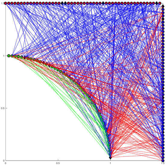
Figure 1.
Illustration of the complex network model. Susceptible individuals are shown as circles and the initially infected individuals are shown as black diamonds. The green circles and black diamonds on the arc represent V nodes, the red circles and black diamonds on the horizontal line represent B nodes, and the blue circles and black diamonds on the vertical line represent T nodes. The colored lines represent the connections between nodes, with the green lines having a weight factor of 1.5, the blues lines 1, and the red lines 2.
2.4. Algorithm Implementation
Based on multi-network theory, we construct mathematical models as follows.
2.4.1. Symmetric Degree Distribution Network
A random network is set up to describe connections between V individuals: starting from the first node, each time a new node is added and connected to m existing nodes with probability p1, T individuals are added to the network by connecting to V individuals with probability p2, and B individuals are added to the network by connecting to V or T individuals with probability p3 in the end. Figure 2 shows the degree distributions in different groups and different network sizes. It shows that the degree distribution is more bell-like in shape as the network sizes N increase, especially in the V group. The T and B degree distributions are similar despite joining the network in a different order. The average degree in the V group is 8, and in the B or T group, it is 6 because there are no connections inside these groups.
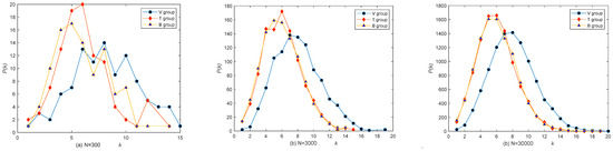
Figure 2.
The degree distribution of the random network. (a) N = 300, (b) N = 3000, and (c) N = 30,000.
2.4.2. Asymmetric Degree Distribution Network
A scale-free network is set up to describe connections between V individuals: starting from a connected network with m0 nodes, each time a new node is added and connected to m existing nodes with probability , ki is the degree of the ith node and m is the average degree; T individuals with the power-law distribution degrees are added to the network by connecting to V individuals with probability , and B individuals with power-law distribution degrees are added to the network by connecting to V or T individuals with probability . Figure 3 shows the result of a simulation; for the network generated by this model, its degree distribution follows a power law distribution as the total number of nodes N is large.
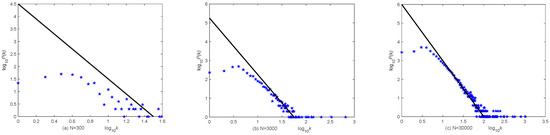
Figure 3.
The degree distribution of the scale-free network. (a) N = 300, (b) N = 3000, and (c) N = 30,000.
2.4.3. Simulation Procedure
At each time step, all connections to the infected node (node i) are found in the network. If the neighboring node (node j) belongs to the susceptible group S, it will be infected with a certain probability , where is the (i, j)-entry of the weighted adjacency matrix, representing the weight factor of the connection from node i to node j. The newly infected node is found and marked as ‘infected’. Table 2 lists the parameters of the model, and based on a survey, it is estimated that the preference ratio in the MSM population is equally divided [27].
Table 2.
The parameters in the model.
Due to the stochasticity involved in the network model, n simulations are carried out, and the average data and relative variance are analyzed as follows
3. Results
3.1. Stochasticity in the Network
Network models involve stochasticity; some papers tend to analyze the average of dozens or hundreds of calculations, but if the variance is significant, individual simulation results will be different from the average.
3.1.1. Stochasticity in the Symmetric Degree Distribution Network
A random network is set up comprising 300 nodes equally divided into the V group (the average degree is 8), T group (the average degree is 6), and B group (the average degree is 6). Figure 4a shows six calculations (with different labels and colors) in the same network and the average of these calculations (as shown by a black line). This process is repeated three times, and the result is shown in Figure 4b, where the black line, blue dashed line, and red dot represent the average value of the six calculations. Figure 4c shows the relative variance of each time. Figure 4b,c indicate that six calculations are sufficient to obtain the average. However, due to the variance, a single simulation may differ from the average.
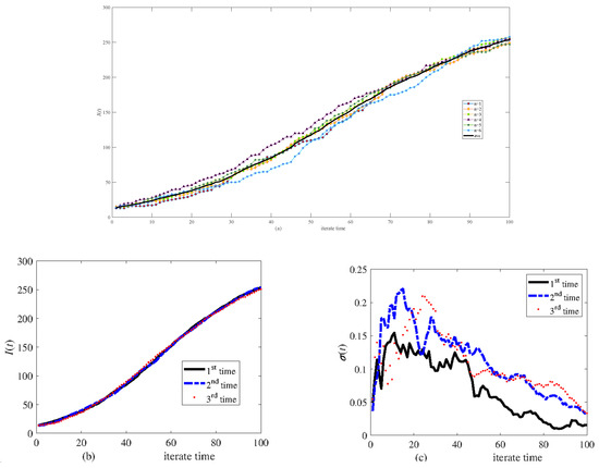
Figure 4.
Simulation results of infective I(t) in the same symmetric network of 300 nodes. (a) Six calculations and their average, (b) the average of six calculations carried out three times, and (c) the relative variance of six calculations.
Figure 4 shows the effect of transmitting stochasticity. Figure 5 displays six calculation results according to six different networks set up based on the same algorithm to explore the effect of network generation stochasticity. Figure 5a shows the results of a simulation. Figure 5b,c show the results of three simulations. The results indicate that although network generation stochasticity has some effect, the transmission of disease is primarily influenced by stochasticity in this process.
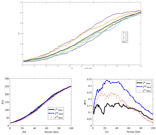
Figure 5.
Simulation results of infective I(t) in different randomly generated networks of 300 nodes. (a) Six calculations and their average, (b) the average of six calculations carried out three times, and (c) the relative variance of six calculations.
Figure 6 shows the stochasticity in both the same network (Figure 6a) and different networks (Figure 6b) of 3000 nodes, which is small, especially in the same network (Figure 6a).
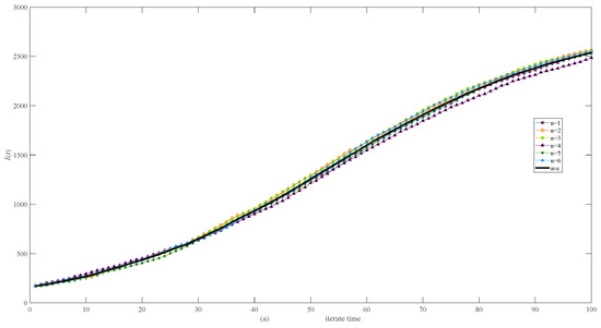
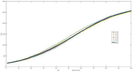
Figure 6.
Simulation results of infective I(t) in randomly generated network of 3000 nodes. (a) Six calculations and their average in the same network. (b) Six calculations and their average in different networks.
3.1.2. Stochasticity in the Asymmetric Degree Distribution Network
The scale-free network of 300 nodes is divided equally into the V group, T group, and B group. Figure 7a shows six calculations and their average in the same network. Figure 7b,c show results that have been repeated three times. Figure 7b,c indicate that six calculations are sufficient to obtain the average. Comparison with Figure 4 shows that the stochasticity in the asymmetric network is more significant than in the symmetric network.

Figure 7.
Simulation results of infective I(t) in the same scale-free network of 300 nodes. (a) Six calculations and their average, (b) the average of six calculations carried out three times, and (c) the relative variance of six calculations.
Figure 8 displays six calculations to six different networks.
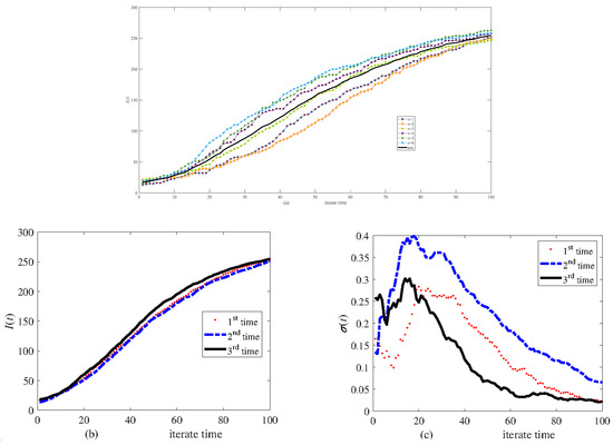
Figure 8.
Simulation results of infective I(t) in different scale-free networks of 300 nodes. (a) Six calculations and their average, (b) the average of six calculations carried out three times, and (c) the relative variance of six calculations.
Figure 9 shows the stochasticity within the same network (Figure 9a) and across different networks (Figure 9b) of 3000 nodes, which is small.
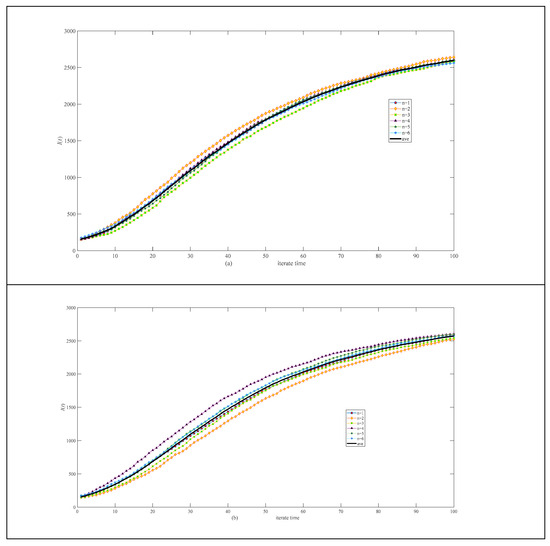
Figure 9.
Simulation results of infective I(t) in a scale-free network of 3000 nodes. (a) Six calculations and their average in the same network. (b) Six calculations and their average in different networks.
3.2. Analysis of Centrality
Based on a randomly generated network of N = 300, the degree vector , the weighted degree vector , the centrality eigenvector , and the weighted centrality eigenvector are obtained using Equations (3)–(5), and (7). They are sorted from largest to smallest, and the sequence numbers are denoted as (the ID of the node with the nth maximum degree), (the id of the node with the nst maximum weighted degree), (the ID of the node of the nth maximum value in the centrality eigenvector) and (the ID of the node of the nth maximum value in the weighted centrality eigenvector).
3.2.1. Centrality of the Symmetric Degree Distribution Network
Table 3 lists the top 20 sequence orders of degree, the degree vector (nk), and the centrality eigenvector (nx) in the symmetric degree distribution network. There are 18 nodes in the top 20 of both the degree vector and the centrality eigenvector. Nodes 248 and 32 are not in the top 20 of the centrality eigenvectors; they are 38th and 45th in the sorted centrality eigenvector, respectively. Nodes 238 and 247 are not in the top 20 of the degree vector; they are 30th and 52nd in the sorted degree vector, and their degrees are 10 and 9, respectively. Although the sequence orders of degree and eigenvector in the randomly generated network are different, this difference is insignificant.
Table 3.
The sequence orders of degree vector and eigenvector centrality in the symmetric degree distribution network.
Table 4 lists the top 20 sequence orders of the weighted degree, the weighted degree vector (), and the weighted centrality eigenvector () in the symmetric degree distribution network. There are 15 nodes in the top 20 of both the weighted degree vector and the weighted centrality eigenvector. Nodes 197, 195, 155, 132, and 18 are in the top 20 of the weighted degree vector, but not in the top 20 of the weighted centrality eigenvectors; nodes 173, 118, 138, 69, and 103 are in the top 20 of the weighted centrality eigenvectors, but not the weighted degree vector.
Table 4.
The sequence orders of the weighted degree vector and weighted eigenvector in the symmetric degree distribution network.
Figure 10 shows the effect of quarantining the top 3 maximum weighted degree nodes (as shown by red circles in Figure 10); there is a very slight difference from the no-quarantine scenario (as shown by the black line in Figure 10).
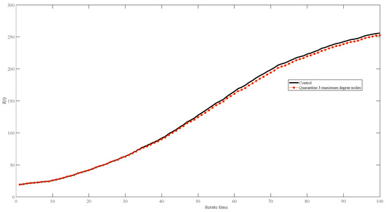
Figure 10.
Simulation results of infective I(t) in networks of quarantine strategies. The black line represents no quarantine, and the red dots represent quarantining the maximum three-degree nodes.
3.2.2. Centrality of the Asymmetric Degree Distribution Network
Table 5 lists the top 20 sequence orders of weighted degree, the weighted degree vector (), and the weighted centrality eigenvector () in the asymmetric degree distribution network. There are 14 nodes in the top 20 of both the weighted degree vector and the weighted centrality eigenvector. Nodes 197, 229, 17, 294, 239, and 18 are in the top 20 of the weighted degree vector, but not in the top 20 of the weighted centrality eigenvectors; nodes 97, 165, 231, 291, 219, and 113 are in the top 20 of the weighted centrality eigenvectors, but not the weighted degree vector.
Table 5.
The sequence orders of the weighted degree vector and weighted eigenvector in the asymmetric degree distribution network.
Based on Table 5, we quarantine different nodes in the top 8 sequence orders, namely the 7th and 8th maximum nodes of the weighted degree vector and the 2nd and 7th maximum nodes of the weighted centrality eigenvector, and compare their results in Figure 11. Our results show that the effect of quarantining the nodes based on the centrality eigenvector is better initially (under the low infective proportion condition), while quarantining the nodes based on the degree eigenvector is better later on (under the high infective proportion condition).
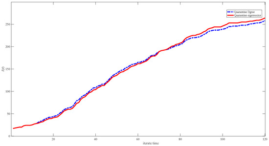
Figure 11.
Simulation results of infective I(t) in networks of different centrality strategies. The blue dashed line represents quarantining the 7th and 8th maximum nodes of the weighted degree vector, and the red line represents quarantining the 2nd and 7th maximum nodes of the weighted centrality eigenvector.
Figure 12 shows the quarantine strategy’s effect when quarantining the top three minimum degree nodes (yellow diamonds in Figure 12); there is no difference from the no-quarantine scenario (shown by the black line in Figure 12), while there is a significant difference when comparing no-quarantine to quarantining the top three maximum degree nodes (shown by red dots in Figure 12).
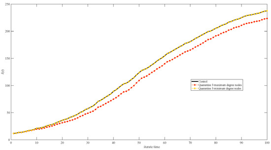
Figure 12.
Simulation results of infective I(t) in networks of different quarantine strategies. The black line represents no quarantine; yellow diamonds represent quarantining the minimum three-degree nodes; and red dots represent quarantining the maximum three-degree nodes.
4. Discussion
4.1. Stochasticity of Complex Networks
Complex networks exhibit stochasticity [29]; the stochasticity in the symmetric degree distribution network (Figure 4, Figure 5 and Figure 6) is lower than that in the asymmetric degree distribution network (Figure 7, Figure 8 and Figure 9). Stochasticity decreases with the increase in N, and the stochasticity is small when N = 3000 (Figure 6 and Figure 9). These results are consistent with those in single networks where stochasticity in the small-world network (symmetric degree distribution) is lower than in the scale-free network [16]. In addition, the stochasticity in multi-interacting networks is higher than in single networks. For the asymmetric degree distribution network (the scale-free network), Figure 7a shows that stochasticity is high when N = 300, while stochasticity is low when N = 200 in a single network [16]. Figure 7b shows that the average values of six simulations are consistent when N = 300; although the variance is significant, six calculations are sufficient to obtain the average value. Figure 4, Figure 5, Figure 7 and Figure 8 compare the effect of disease transmission stochasticity and network generation stochasticity, indicating that disease transmission stochasticity is the primary source.
4.2. Analysis of the Degree Vector and the Centrality Eigenvectors
Both the degree vector and the centrality eigenvector can reflect the characteristics of the network structure. Only a slight difference exists between degree centrality and eigenvector centrality in both symmetric and asymmetric distribution networks. Our simulation results show that regardless of whether the network has a symmetric or an asymmetric degree distribution, only one node is different among the top five maximum values in both the weighted degree vector and the weighted centrality eigenvector. Additionally, we found that there are five different nodes in the top 20 maximum values (as shown in Table 4 and Table 5). In the asymmetric degree distribution network, compared with quarantining the top three minimum degree nodes, quarantining the top three maximum degree nodes will reduce disease transmission; therefore, quarantining the central node is an effective method for controlling disease transmission.
Comparing the quarantining results of different IDs of the top 20 degree vectors and the centrality eigenvector shows that the centrality eigenvector strategy performs better initially, while the central degree strategy shows improved results later on. Two factors infect the centrality eigenvector: the node’s degree and its connections’ degrees. We can assume that at the beginning, most of the nodes are uninfected. Quarantining the centrality eigenvector strategy can help block transmission to the uninfected node of large degree; but over time, most of the nodes become infected, and quarantining the node that connects to node of large degree is no longer a suitable method because the connecting node may have already been infected; therefore, directly quarantining the node of large degree is more effective.
4.3. Comparison Between Symmetric and Asymmetric Distribution Networks
The degree distribution of the random network is symmetric, and the degrees are mainly concentrated around the mean degree (Figure 2). The degree distribution of the scale-free network is severely asymmetric, resulting in some nodes with very large degrees (Figure 3); random variations in these nodes will significantly impact the results, both for the different simulation processes and the different network generations. Therefore, the stochasticity in the scale-free network (Figure 7, Figure 8 and Figure 9) seems higher than in the random network (Figure 4, Figure 5 and Figure 6). Unlike in the scale-free network (depicted by the red dot in Figure 12), quarantining the top three maximum degree nodes has minimal effect on disease transmission (depicted by the red dot in Figure 10), which means that quarantining the central node may not be effective in the random network.
5. Conclusions
In complex networks, the average of multiple results tends to be constant when N is large enough, but a single simulation is still stochastic. Therefore, when studying complex network problems, it is important to consider this uncertainty. Moreover, the stochasticity in asymmetric networks is more significant than in symmetric networks. Therefore, unexpected results are more likely to occur in asymmetric networks. In general, eigenvector centrality tends to reflect degree centrality, e.g., articles with a high-eigenvector centrality tend to be highly cited articles [30], and high-degree nodes have a significant impact on propagation. Because the degree of a node is easier to obtain than the eigenvector [31], degree centrality analysis may be preferred for such problems. However, in some domains, such as power supply, interconnection networks, transportation networks, etc., some low-degree nodes may serve as key connecting nodes between two sub-networks within the whole network [32]. Thus, employing eigenvector centrality analysis may prove more effective.
Author Contributions
G.W.: Conceptualization, Data curation, Validation, Writing—original draft, review & editing. W.Y.: Methodology, Software, Project administration, Funding acquisition, Writing—review & editing. All authors have read and agreed to the published version of the manuscript.
Funding
This research was funded by the National Natural Science Foundation of China (grant number: 12172092) and Shanghai Key Laboratory of Acupuncture Mechanism and Acupoint Function (grant number: 21DZ2271800).
Data Availability Statement
Data will be made available on request.
Conflicts of Interest
The authors declare no conflicts of interest.
References
- Boccaletti, S.; Latora, V.; Moreno, Y.; Chavez, M.; Hwang, D.U. Complex networks: Structure and dynamics. Phys. Rep. 2006, 424, 175–308. [Google Scholar] [CrossRef]
- Boccaletti, S.; Almendral, J.A.; Guan, S.; Leyva, I.; Liu, Z.; Sendina-Nadal, I.; Wang, Z.; Zou, Y. Explosive transitions in complex networks’ structure and dynamics: Percolation and synchronization. Phys. Rep. 2016, 660, 1–94. [Google Scholar] [CrossRef]
- Estrada, E. Introduction to Complex Networks: Structure and Dynamics. Evol. Equ. Appl. Nat. Sci. 2015, 2126, 93–131. [Google Scholar] [CrossRef]
- Watts, D.J.; Strogatz, S.H. Collective dynamics of ‘small-world’ networks. Nature 1998, 393, 440–442. [Google Scholar] [CrossRef] [PubMed]
- Barabasi, A.L.; Albert, R. Emergence of scaling in random networks. Science 1999, 286, 509–512. [Google Scholar] [CrossRef] [PubMed]
- Yan, C. Network Model with Scale-Free, High Clustering Coefficients, and Small-World Properties. J. Appl. Math. 2023, 2023, 5533260. [Google Scholar] [CrossRef]
- Liljeros, F.; Edling, C.R.; Amaral, L.; Stanley, H.E.; Åberg, Y. The web of human sexual contacts. Nature 2001, 411, 907–908. [Google Scholar] [CrossRef] [PubMed]
- Restrepo, J.G.; Ott, E.; Hunt, B.R. Characterizing the dynamical importance of network nodes and links. Phys. Rev. Lett. 2006, 97, 94102. [Google Scholar] [CrossRef] [PubMed]
- Bonacich, P. Some unique properties of eigenvector centrality. Soc. Netw. 2007, 29, 555–564. [Google Scholar] [CrossRef]
- Zheng, Q.; Shen, J.; Pandey, V.; Guan, L.; Guo, Y. Turing instability in a network-organized epidemic model with delay. Chaos Solitons Fractals 2023, 168, 113205. [Google Scholar] [CrossRef]
- Shen, D.; Li, J.H.; Zhang, Q.; Zhu, R. Interlacing layered complex networks. Acta Phys. Sin.-Chin. Ed. 2014, 63, 190201. [Google Scholar] [CrossRef]
- Kurant, M.; Thiran, P. Layered complex networks. Phys. Rev. Lett. 2006, 96, 138701. [Google Scholar] [CrossRef]
- Tyloo, M. Layered complex networks as fluctuation amplifiers. J. Phys.-Complex. 2022, 3, 3. [Google Scholar] [CrossRef]
- Zhou, Y. Numerical Study of the Effective Degree Theory on Two- Layered Complex Networks. In Proceedings of the Iecon 2017—43rd Annual Conference of the IEEE Industrial Electronics Society, Beijing, China, 29 October–1 November 2017; pp. 5912–5917. [Google Scholar]
- Jeffries, W.T. The number of recent sex partners among bisexual men in the United States. Perspect. Sex. Reprod. Health 2011, 43, 151–157. [Google Scholar] [CrossRef]
- Wang, G.; Yao, W. An application of complex networks on predicting the behavior of infectious disease on campus. Math. Methods Appl. Sci. 2024, 48, 189–206. [Google Scholar] [CrossRef]
- Wang, G.; Yao, W. An application of small-world network on predicting the behavior of infectious disease on campus. Infect. Dis. Model. 2024, 9, 177–184. [Google Scholar] [CrossRef]
- Yang, J.; Cao, Z.; Lu, Y. Contagion dynamics on a compound model. Appl. Math. Comput. 2024, 460, 128293. [Google Scholar] [CrossRef]
- Saumell-Mendiola, A.; Serrano, M.A.; Boguna, M. Epidemic spreading on interconnected networks. Phys. Rev. E 2012, 86, 026106. [Google Scholar] [CrossRef]
- Saha, S.; Samanta, G.P. Modelling and optimal control of HIV / AIDS prevention through PrEP and limited treatment. Phys. A 2019, 516, 280–307. [Google Scholar] [CrossRef]
- Vieira, I.T.; Cheng, R.C.H.; Harper, P.R.; de Senna, V. Small world network models of the dynamics of HIV infection. Ann. Oper. Res. 2010, 178, 173–200. [Google Scholar] [CrossRef]
- Lou, J.; Wu, J.; Chen, L.; Ruan, Y.; Shao, Y. A sex-role-preference model for HIV transmission among men who have sex with men in China. BMC Public Health 2009, 9, S10. [Google Scholar] [CrossRef] [PubMed]
- Shen, Z.; Li, Y.; Yao, W. A scale-free network model for HIV transmission among men who have sex with men in China. Math. Methods Appl. Sci. 2016, 39, 5131–5139. [Google Scholar] [CrossRef]
- Zhong, C.; Sun, M.; Yao, W. A hybrid model for HIV transmission among men who have sex with men. Infect. Dis. Model. 2020, 5, 814–826. [Google Scholar] [CrossRef]
- Bonacich, P. Power and centrality—A family of measures. Am. J. Sociol. 1987, 92, 1170–1182. [Google Scholar] [CrossRef]
- Xie, L.; Yao, W. A network-based study on HIV spreading among men who have sex with men. Chin. Sci. Bull. (Chin. Ver.) 2013, 58, 1731–1738. [Google Scholar]
- Yee, N. Beyond Tops and Bottoms: Correlations between Sex-Role Preferences and Physical Preferences for Partners among Gay Men. 2002. Available online: http://www.nickyee.com/ponder/topbottom.pdf (accessed on 16 January 2025).
- Wang, S.T.; News, S.D. China’s Gay Men’s HIV Infection Rate Reaches 4.9%, Becoming a Key Population Group for Transmission. Available online: https://www.chinanews.com/jk/kong/news/2008/12-02/1470137.shtml (accessed on 14 January 2025). (In Chinese).
- Tocino, A.; Serrano, D.H.; Hernandez-Serrano, J.; Villarroel, J. A stochastic simplicial SIS model for complex networks. Commun. Nonlinear Sci. 2023, 120, 107161. [Google Scholar] [CrossRef]
- Li, Z.; Jiang, M.Y.; Liu, X.; Cai, Y.; Wang, C.; Cao, F.; Liu, J. Research trends of acupressure from 2004 to 2024: A bibliometric and visualization analysis. Heliyon 2024, 10, e38675. [Google Scholar] [CrossRef] [PubMed]
- Zhang, Y.; Wang, M.; Saberi, M.; Chang, E. Analysing academic paper ranking algorithms using test data and benchmarks: An investigation. Scientometrics 2022, 127, 4045–4074. [Google Scholar] [CrossRef]
- Buldyrev, S.V.; Parshani, R.; Paul, G.; Stanley, H.E.; Havlin, S. Catastrophic cascade of failures in interdependent networks. Nature 2010, 464, 1025–1028. [Google Scholar] [CrossRef] [PubMed]
Disclaimer/Publisher’s Note: The statements, opinions and data contained in all publications are solely those of the individual author(s) and contributor(s) and not of MDPI and/or the editor(s). MDPI and/or the editor(s) disclaim responsibility for any injury to people or property resulting from any ideas, methods, instructions or products referred to in the content. |
© 2025 by the authors. Licensee MDPI, Basel, Switzerland. This article is an open access article distributed under the terms and conditions of the Creative Commons Attribution (CC BY) license (https://creativecommons.org/licenses/by/4.0/).