Dynamic Value at Risk Estimation in Multi-Functional Volterra Time-Series Model (MFVTSM)

Abstract

In this paper, we aim to provide a new algorithm for managing financial risk in portfolios containing multiple high-volatility assets. We assess the variability of volatility with the Volterra model, and we construct an estimator of the Value-at-Risk (VaR) function using quantile regression. Because of its long-memory property, the Volterra model is particularly useful in this domain of financial time series data analysis. It constitutes a good alternative to the standard approach of Black–Scholes models. From the weighted asymmetric loss function, we construct a new estimator of the VaR function usable in Multi-Functional Volterra Time Series Model (MFVTSM). The constructed estimator highlights the multi-functional nature of the Volterra–Gaussian process. Mathematically, we derive the asymptotic consistency of the estimator through the precision of the leading term of its convergence rate. Through an empirical experiment, we examine the applicability of the proposed algorithm. We further demonstrate the effectiveness of the estimator through an application to real financial data.

1. Introduction

In financial mathematics, stochastic integral equations are usually used to fit memory effects and model the movement of financial assets. These stochastic equations are useful for modeling volatility clustering, rough volatility, or heavytail characteristics of financial data. In the present work we aim to evaluate financial risk by modeling historical data as a continuous, multidimensional process sampled from MFVTSM. Such a research topic is primarily motivated by the long-memory feature of the Volterra model, which is a critical factor in financial time-series analysis. Even if the bibliography on the multivariate analysis of the model is very abundant, the functional path of this kind of model is not fully explored. For the first development of this topic, we mention Ref. [1]. The cited reference enhances stochastic volatility models by incorporating long-memory kernels, which permits improvement in the efficiency of the financial modeling. The authors of Ref. [2] use Volterra-type equations to study volatility surfaces. Ref. [3] introduces the rough Heston model to improve derivative pricing. This last method employs the Volterra model to fit rough volatility effects. For a deeper discussion on the role of non-Markovian processes in financial markets, we refer to [4]. Such pioneering works highlight the crucial role of the Volterra model in the improvement of pricing precision and volatility calibration, as well as risk management. At this stage, evaluating financial risk through historical data remains a challenging issue for bankers and investors. The VaR function is commonly used to remedy this issue. The statistical estimation of the VaR function is commonly based on the unconditional quantile function. However, the conditional quantile is more appropriate for monitoring the dynamics of financial transactions. Pioneering investigations in the conditional VaR were conducted by [5], who consider the VaR estimation under a conditional autoregressive model. Since this cited work, significant progress in risk management using conditional (CAVaR) models has been observed. For instance, ref. [6] conducted a comprehensive comparative analysis between traditional VaR and a hybrid method that combines GARCH modeling with extreme value theory. Their work provides valuable ideas into the relative performance of these risk measurement techniques. In a related study, ref. [7] investigated the optimal order selection for VaR estimation, offering an important methodological algorithm to the specification of VaR models. There exist many alternative approaches to estimate the conditional VaR by a parametric approach. We mention the GARCH approach in ref. [8], Extreme Value (EV) by [9], and the conditional copula [10], among others. The estimation of quantile regression is widely considered in mathematical statistics. The pioneering work in a multivariate case was developed by [11]. The latter constructed an estimator using an empirical estimator of the conditional distribution function. Next, ref. [12] derived the asymptotic normality of the nonparametric conditional quantile estimator. For a comprehensive review of the literature on quantile regression, we refer to [13]. Furthermore, the functional version of quantile regression was introduced by [14]. The authors have used B-spline smoothing to study a linear quantile regression model with Hilbertian explanatory variables. They also derived the $L_2$-convergence rate of their estimator. Nonparametric smoothing was considered by [15]. The latter proved the almost-complete convergence (a.co.) of a kernel estimator of quantile regression. Ref. [16] proposed a local linear estimation method for functional quantiles by inverting the local linear estimator of the conditional cumulative distribution function. Subsequently, ref. [17] studied the partial linear quantile regression, with particular attention to handling incomplete data cases. As an alternative approach, ref. [18] developed a functional partial quantile estimator using basis expansion techniques. More recently, ref. [19] introduced a robust estimation procedure for scalar-on-function quantile regression models that effectively handles outliers while maintaining prediction reliability. Despite its significance, research on multivariate functional data remains relatively scarce. To the best of our knowledge, only one reference [20] has addressed the estimation of unconditional quantiles in the context of multi-functional statistics.

As an alternative development to the cited works, we aim in this contribution to treat the conditional quantile case under multi-functional data. Under this consideration we construct an estimator and we establish its complete consistency. Moreover, we use this model to provide a new approach to assessing financial risk using a Gaussian Volterra chaotic model. The particularity of the introduced algorithm is the treatment of financial data as a continuous Gaussian Volterra process, which allows it to reflect the nature of financial time-series data. This approach is especially powerful for modeling memory effects and path-dependent market behaviors. Indeed, it is well known that the model’s kernel is adequate to detect the local interactions and long-range dependencies which are very beneficial to describe real-world market characteristics such as rough volatility, cluster effects, and heavy-tailed distributions. In this context the Volterra model has proven useful across various financial applications, from derivative pricing to the calibration of volatility surface and risk management. Additionally, the Volterra model offers a more robust alternative to the standard Black–Scholes framework, which suffers from several practical limitations. The most significant is Black–Scholes’s assumption of constant volatility and interest rates, an overly simplistic view that does not accurately represent real market conditions. Instead, the Volterra model accounts for fluctuating volatility and memory effects, allowing a more adaptable illustration of market dynamics. On the other hand, we have used nonparametric estimation techniques, which provide flexibility in modeling financial dynamics without relying on rigid assumptions. Typically, for financial time-series data analysis nonparametric functional data modeling permits the user to fit the dynamic of high-frequency and high-dimensional relationships of the data that traditional multivariate GARCH models fail to incorporate. More precisely, unlike standard multivariate GARCH models, which are based on some specific assumptions (linearity and limited discrete time-point observations), functional statistics offer a flexible approach to model the entire historical trajectory of financial data as continuous curves. Thus, the nonparametric functional approach allows a deeper understanding of time-varying volatility, risk spread, and non-linear time-varying dependencies. Therefore, the principal advantage of the present contribution is the multi-functional treatment offering a robust, data-driven alternative for risk management and portfolio optimization and enhancing the accuracy via the VaR model for more complex markets. Finally, we point out that all these advantages have been highlighted through simulation and real data application after establishing the mathematical consistency of the constructed estimator.

The paper is structured as follows: Section 2 introduces the general framework of the contribution. In Section 3, we present and discuss the main results. Section 4 focuses on the empirical study, which includes both simulated and real data applications. In the Section 5, we provide a general conclusion along with some research perspectives for future work. Finally, the Appendix A contains the proofs of supporting results.

2. Methodology

2.1. Multifunctional Data Framework

In this paper we assume that we have a portfolio of d financial assets; each one has trajectory $T_i(·)$, which behaves as a Gaussian Volterra process such that

$$T^i\left(s\right)={\int }_0^t\mathfrak{L}(t,s)d{B}^i\left(t\right),i=1,\dots ,d,s\in [0,1],\mathrm{and} \mathfrak{L}\mathrm{is} \mathrm{a} \mathrm{kernel}.$$

The dynamic of the portfolio is formulated as

$$T\left(s\right)=\left(\begin{array}{c}{T}^1\left(s\right)\\ T^2\left(s\right)\\ ⋮\\ T^d\left(s\right)\end{array}\right)$$

This setting is common in financial mathematics. Its popularity is justified by the long memory of stock market dynamics (see [21]). In this functional framework, we employ the Cameron–Martin space defined as follows:

$$\mathcal{H}=\{functionf\left(s\right)={\int }_0^s\mathfrak{L}(t,s)h_f\left(t\right)dt \mathrm{for} t\in [0,1]\mathrm{and} h_f\in L^2\left([0,1]\right)\}.$$

The space $\mathcal{H}$ carries the scalar product $<f,g>=<h_f,h_g{>}_{L^2\left([0,1]\right)}$ and an orthonormal basis

$$f_n\left(s\right)={\int }_0^t\mathfrak{L}(t,s)h_n\left(s\right)dt,t\in (0,1)\left(h_n\right)\mathrm{is} \mathrm{an} \mathrm{orthonormal} \mathrm{basis}{L}^2\left([0,1]\right).$$

The main objective of this paper is to assess the long-term risk in financial asset movements using historical data. The primary contribution of this work is the exploration of the historical information of multiple returns in a continuous form. Indeed, we sample N multi-functional variables as covariates ${\left({\mathcal{C}}_k\right)}_{k=1,2,\dots ,N}$ defined as follows:

$$\forall s\in [0,1],{\mathcal{C}}_k^i\left(s\right)=T^i\left({\displaystyle \frac{(k-1)+t}{N}}\right)i=1,2,\dots d.$$

(1)

The financial risk is assessed with respect to the future characteristics of the portfolio’s returns. Among the principal characteristics are minimum or maximum values, daily range, variation over fixed periods, closed values, and values at a given time $t_0$, among others. Mathematically, we represent the future characteristics through a function $Fu$. This last function defines the intersect variables ${\left({\mathcal{S}}_k\right)}_{k=1,2,\dots ,N}$ as follows:

$${\mathcal{S}}_k=Fu\left({\mathcal{C}}_k^i\right),i=1,2,\dots d.k=1,2,\dots ,N,$$

(2)

Finally, we analyze the financial dynamic using $Z_k={({\mathcal{C}}_k,{\mathcal{S}}_k)}_{k=1,2,\dots ,N}$ as multi-functional random variable drown from Volterra process defined in (1) and (2).

2.2. Model and Estimation

The present contribution focuses on the estimation of the VaR function as a solution of the following optimization problem:

$$\begin{array}{c}Q{P}_p\left(\mathcal{V}\right)=\arg \underset{y\in \mathbb{R}}{\min }\left\{\mathbb{E}\left[p(\mathcal{S}-y)1{\mathrm{I}}_{\left\{\right(\mathcal{S}-y)>0\}}\mid \mathcal{C}=\mathcal{V}\right]\right.\hfill \\ \left.+\mathbb{E}\left[(1-p)(\mathcal{S}-y)1{\mathrm{I}}_{\left\{\right(\mathcal{S}-y)\le 0\}}\mid \mathcal{C}=\mathcal{V}\right]\right\},p\in (0,1),\mathcal{V}=\left(\begin{array}{c}{\mathcal{V}}^1\\ {\mathcal{V}}^2\\ ⋮\\ {\mathcal{V}}^d\end{array}\right)\in \mathcal{H}\hfill \end{array}$$

(3)

It is important to note that the scoring function in this optimization problem is convex, with limit $+\infty$ at both $-\infty$ and $+\infty$ (with great probability); it has at least one minimizing value over $\mathbb{R}$. It should also be noted that this scoring function is piecewise linear with monotonically increasing slope and may include a flat segment (where the slope is zero) corresponding to its minimum value. In this situation, we take $Q{P}_p\left(\mathcal{V}\right)$ as the smallest minimizing value. Otherwise, ${\widehat{t}}_p\left(x\right)$ is unique and locates the turning point from negative to positive slope. Furthermore, it is shown in ref. [22] that $Q{P}_p\left(\mathcal{V}\right)$ is the root of

$$\begin{array}{c}{\displaystyle \mathcal{F}(y,\mathcal{V})-p=0,}\hfill \end{array}$$

(4)

where

$${\mathcal{F}}_{(}y,\mathcal{V})=\mathbb{E}\left[1{\mathrm{I}}_{\left\{\right(\mathcal{S}-y)\le 0\}}\mid I=\mathcal{V}\right]$$

Now, the quantity $Q{P}_p\left(\mathcal{V}\right)$ is estimated $\widehat{Q{P}_p}\left(\mathcal{V}\right)$ as the zero of

$$\widehat{\mathcal{F}}(y,\mathcal{V})-p=0$$

(5)

with

$$\widehat{\mathcal{F}}(y,\mathcal{V})={\displaystyle \frac{{\displaystyle {\Sigma }_{k=1}^N\prod _{i=1}^d\mathbf{K}(a^{-1}\parallel {\mathcal{V}}^i-{\mathcal{C}}_k^i\parallel )1{\mathrm{I}}_{\{({\mathcal{S}}_k-y)\le 0\}}}}{{\displaystyle {\Sigma }_{k=1}^N\prod _{i=1}^d\mathbf{K}(a^{-1}\parallel {\mathcal{V}}^i-{\mathcal{C}}_k^i\parallel )}}},$$

where $\mathbf{K}$ is given a measurable kernel, a is a sequence of positive numbers, and $\parallel ·\parallel$ is $L^2(0,1)$-norm.

Of course, the applicability of the risk detector $\widehat{Q{P}_p}\left(\mathcal{V}\right)$ necessitates a theoretical foundation to establish the conditions for its optimality.

3. The Mathematical Foundation of the Estimation

3.1. Assumptions

Hereafter, for $\mathcal{V}\in \mathcal{H}$, we set by $N_{\mathcal{V}}$ neighborhood of $\mathcal{V}$, and $c_1,c_2,c_{,}\dots$ are positive constants. Furthermore, we set

$$B(\mathcal{V},a)=\left\{{\mathcal{V}}^{\prime }\in \mathcal{H}:{\Sigma }_{i=1}^d\parallel {{\mathcal{V}}^{\prime }}^i-{\mathcal{V}}^i\parallel <a\right\}.$$

We need the following assumptions:

(As1)

The functions $\mathcal{F}(·,\mathcal{V})$ are differentiable in $\mathbb{R}$ and satisfy the following:

$$\exists h>0\forall y\in \left[Q{P}_p\left(\mathcal{V}\right)-h,Q{P}_p\left(\mathcal{V}\right)+h\right],\forall {\mathcal{V}}_1,{\mathcal{V}}_2\in \mathcal{F},$$

$$|\mathcal{F}(y,{\mathcal{V}}_1)-\mathcal{F}(y,{\mathcal{V}}_2)|\le c_1{\Sigma }_{i=1}^d{\parallel {\mathcal{V}}_1^i-{\mathcal{V}}_2^i\parallel }^{b_1},\mathrm{with}{\displaystyle \frac{\partial \mathcal{F}(Q{P}_p\left(\mathcal{V}\right),\mathcal{V})}{\partial y}}>0$$

(As2)

The function $\mathfrak{L}(·,·)$ is a Holder continuous kernel such that

$$\left\{\begin{array}{c}\left(i\right)\mathrm{The} \mathrm{map} t\to \mathfrak{L}(t,s)\mathrm{is} \mathrm{differentiable} \mathrm{on}t\hfill \\ \mathrm{and} \mathrm{has} \mathrm{derviative} L^2-\mathrm{integrable}\hfill \\ \mathrm{such} \mathrm{that}\underset{0\le s<t\le 1}{max}\left|{\displaystyle \frac{\partial \mathfrak{L}(t,s)}{\partial t}}\right|{(t-s)}^{3/2}<\infty .\hfill \\ \left(ii\right)\mathrm{The} \mathrm{map} t\to {\int }_0^t\mathfrak{L}(t,s)ds\mathrm{has} \mathrm{bounded} \mathrm{variation}.\hfill \end{array}\right.$$

(As3)

For all $a>0$, and $\nu >1/2$ we suppose that $\mathrm{I}\mathrm{P}\left(I\in B(\mathcal{V},a)\right)=\zeta (d,\mathcal{V},a)>0$ and for all ${\displaystyle i\ne j}$,

$$\underset{i\ne j}{sup}\mathrm{I}\mathrm{P}\left[({\mathcal{C}}_j,{\mathcal{C}}_i)\in B(\mathcal{V},a)\times B(\mathcal{V},a)\right]=O((\zeta {(d,\mathcal{V},a)}^{1+{\displaystyle \frac{\nu }{\nu +1}}})),\mathrm{and}{\eta }_{\xi }=e^{-\nu \xi }.$$

(As4)

There exist $c_1,c_2>0$, such that

$${\displaystyle \frac{log{N}^5}{N^{1-c_1}}}\le \zeta (d,\mathcal{V},a)\le {\displaystyle \frac{1}{log{N}^{1+c_2}}}.$$

(As5)

The function $\mathbf{K}(·)$ has a support $[0,1]$ and satisfies

$$0<c_4\le \mathbf{K}(·)\le c_5<\infty ;c_4,c_5>0$$

Some Comments

The assumed conditions are not restrictive. They allow us to address multiple aspects of the subject (model structure, data characteristics, correlation, and convergence rate). In this context, the imposed assumptions are not overly restrictive, given the complexity of the proposed functional time-series model and the strength of the Borel–Cantelli (BC) consistency result. We point out that not all of these assumptions are strictly necessary for financial data applications; rather, they are required to explore different dimensions of the topic. Specifically, each aspect of the subject is examined through a distinct assumption. For instance, (As1) defines the nonparametric model, while (As2) characterizes the Gaussian Volterra model and is used to identify the orthonormality of the basis function. The functionality of the input variable $\mathcal{C}$ is controlled by (As3), which relates the spectral measure to the Hilbert structure of the input variable as well as its local dependency. The rest of the assumptions are technical and cover the kernel function and the bandwidth sequence, both of which are crucial in determining the convergence rate of the kernel estimator $\widehat{Q{P}_p}\left(\mathcal{V}\right)$ with respect to the Borel–Cantelli mode. In fact, an alternative form of consistency—weaker than BC consistency—can be established for the estimator without these assumptions. Specifically, by computing the expectation and variance of the estimator, we can prove the probability consistency. Although this probability consistency is less than the Borel–Cantelli consistency, it is sufficient to support the practical use of the estimator. However, since this paper seeks to highlight both the theoretical generality of the model and its practical feasibility, we have opted to focus on the stronger consistency result, from which the weaker form naturally follows.

3.2. Asymptotic Result

Now, we can present our main results concerning the asymptotic properties of the estimator $\widehat{Q{P}_p}\left(\mathcal{V}\right)$ under the above assumptions:

Theorem 1.

Under (As1)–(As5), we have

$$\left|\widehat{Q{P}_p}\left(\mathcal{V}\right)-Q{P}_p\left(\mathcal{V}\right)\right|=O_{a.co.}\left(a^{b_1}+\sqrt{{\displaystyle \frac{logN}{N\zeta (d,\mathcal{V},a)}}}\right).$$

(6)

Proof. 

As $\mathcal{F}(y,\mathcal{V}))$, is increasing function, therefore,

$${\displaystyle {\Sigma }_{n\ge 1}\mathrm{I}\mathrm{P}\left(|\widehat{Q{P}_p}\left(\mathcal{V}\right)-Q{P}_p\left(\mathcal{V}\right)|>ϵ\right)}$$

$${\displaystyle \le {\Sigma }_{n\ge 1}\mathrm{I}\mathrm{P}\left(\left|\widehat{\mathcal{F}}(Q{P}_p\left(\mathcal{V}\right)-ϵ,\mathcal{V})-\mathcal{F}(Q{P}_p\left(\mathcal{V}\right)-ϵ,\mathcal{V})\right|\ge |\mathcal{F}(Q{P}_p\left(\mathcal{V}\right),\mathcal{V})-\mathcal{F}(Q{P}_p\left(\mathcal{V}\right)-ϵ,\mathcal{V})|\right)}$$

$${\displaystyle +{\Sigma }_{n\ge 1}\mathrm{I}\mathrm{P}\left(\left|\widehat{\mathcal{F}}(Q{P}_p\left(\mathcal{V}\right)+ϵ,\mathcal{V})-\mathcal{F}(Q{P}_p\left(\mathcal{V}\right)+ϵ,\mathcal{V})\right|\ge \left|\mathcal{F}\right(Q{P}_p(\left(\mathcal{V}\right),\mathcal{V})-\mathcal{F}(Q{P}_p\left(\mathcal{V}\right)+ϵ,\mathcal{V})|\right).}$$

The function $\mathcal{F}(·.\mathcal{V})$ is of class $C^1$ and such that ${\displaystyle \frac{\partial \mathcal{F}(Q{P}_p\left(\mathcal{V}\right),\mathcal{V})}{\partial y}}>0$. Then

$$\exists \delta >0\mathrm{such}\mathrm{that}\underset{y\in [Q{P}_p\left(\mathcal{V}\right)-\delta ,Q{P}_p\left(\mathcal{V}\right)+\delta ]}{inf}{\displaystyle \frac{\partial \mathcal{F}(Q{P}_p\left(\mathcal{V}\right),\mathcal{V})}{\partial y}}\ge C>0.$$

Therefore

$${\Sigma }_{n\ge 1}\mathrm{I}\mathrm{P}\left(|\widehat{Q{P}_p}\left(\mathcal{V}\right)-Q{P}_p\left(\mathcal{V}\right)|>ϵ\right)\le {\Sigma }_N\mathrm{I}\mathrm{P}\left(\underset{y\in [Q{P}_p\left(\mathcal{V}\right)-\delta ,Q{P}_p\left(\mathcal{V}\right)+\delta ]}{sup}|\widehat{\mathcal{F}}(y,\mathcal{V})-\mathcal{F}(y,\mathcal{V})|\ge Cϵ\right).$$

Finally, it suffices

$${\Sigma }_N\mathrm{I}\mathrm{P}\left(\underset{y\in [Q{P}_p\left(\mathcal{V}\right)-\delta ,Q{P}_p\left(\mathcal{V}\right)+\delta ]}{sup}|\widehat{\mathcal{F}}(y,\mathcal{V})-\mathcal{F}(y,\mathcal{V})|\ge C{ϵ}_0\left(a^{k_0}+\sqrt{{\displaystyle \frac{logn}{N\zeta (d,\mathcal{V},a)}}}\right)\right)<\infty .$$

(7)

The latter is based on

$$\begin{array}{ccc}\hfill \widehat{\mathcal{F}}(y,\mathcal{V})-\mathcal{F}(y,\mathcal{V})& =& {\displaystyle \frac{{\displaystyle {\tilde{\mathcal{F}}}_1(y,\mathcal{V})}}{{\displaystyle {\tilde{\mathcal{F}}}_2(y,\mathcal{V})}}}-\mathcal{F}(y,\mathcal{V})\hfill \\ & =& {\displaystyle \frac{{\displaystyle 1}}{{\displaystyle {\tilde{\mathcal{F}}}_2(y,\mathcal{V})}}}\left[{\tilde{\mathcal{F}}}_1(y,\mathcal{V})-\mathcal{F}(y,\mathcal{V})\right]\hfill \\ & & +{\displaystyle \frac{{\displaystyle \mathcal{F}(y,\mathcal{V})}}{{\displaystyle {\tilde{\mathcal{F}}}_2(y,\mathcal{V})}}}\left[{\mathcal{F}}_2(y,\mathcal{V})-1\right],\hfill \end{array}$$

(8)

where

$${\tilde{\mathcal{F}}}_1(y,\mathcal{V})={\displaystyle \frac{1}{N\mathrm{I}\mathrm{E}[{\prod }_{i=1}^d\mathbf{K}(a^{-1}\parallel {\mathcal{V}}^i-I^i\parallel \left)\right]}}{\Sigma }_{k=1}^N\prod _{i=1}^d\mathbf{K}(a^{-1}\parallel {\mathcal{V}}^i-{\mathcal{C}}_k^i\parallel )1{\mathrm{I}}_{\{({\mathcal{S}}_k-y)\le 0},$$

and

$${\tilde{\mathcal{F}}}_2\left(\mathcal{V}\right)={\displaystyle \frac{1}{N\mathrm{I}\mathrm{E}[{\prod }_{i=1}^d\mathbf{K}(a^{-1}\parallel {\mathcal{V}}^i-I^i\parallel \left)\right]}}{\Sigma }_{k=1}^N\prod _{i=1}^d\mathbf{K}(a^{-1}\parallel {\mathcal{V}}^i-{\mathcal{C}}_k^i\parallel ).$$

Consequently, the proof of the main result is based in the following intermediate results. □

Lemma 1.

Under Assumptions (As2)–(As5), we have

$$\underset{y\in [Q{P}_p\left(\mathcal{V}\right)-\delta ,Q{P}_p\left(\mathcal{V}\right)+\delta ]}{sup}\left|{\tilde{\mathcal{F}}}_1(y,\mathcal{V})-\mathrm{I}\mathrm{E}\left[{\tilde{\mathcal{F}}}_1(y,\mathcal{V})\right]\right|=O_{a.co.}\left(\sqrt{{\displaystyle \frac{logN}{N\zeta (d,\mathcal{V},a)}}}\right),$$

(9)

and

$$\left|{\tilde{\mathcal{F}}}_2\left(\mathcal{V}\right)-\mathrm{I}\mathrm{E}\left[{\tilde{\mathcal{F}}}_2\left(\mathcal{V}\right)\right]\right|=O_{a.co.}\left(\sqrt{{\displaystyle \frac{logN}{N\zeta (d,\mathcal{V},a)}}}\right).$$

(10)

Lemma 2.

Assume that the hypotheses (As2), (As4), and (As6) are fulfilled, then

$$\left|\mathrm{E}\left[{\tilde{\mathcal{F}}}_1(y,\mathcal{V})\right]-\mathcal{F}(y,\mathcal{V})\right|=O\left(a^{b_1}\right).$$

(11)

Lemma 3.

Under the hypotheses of Lemma 1, we have

$${\displaystyle \exists {ϵ}_0>0such that{\Sigma }_{N\ge 1}\mathrm{I}\mathrm{P}\left(\left|{\widehat{\mathcal{F}}}_2\left(\mathcal{V}\right)\right|\le {ϵ}_0\right)<\infty .}$$

(12)

4. Empirical Analysis

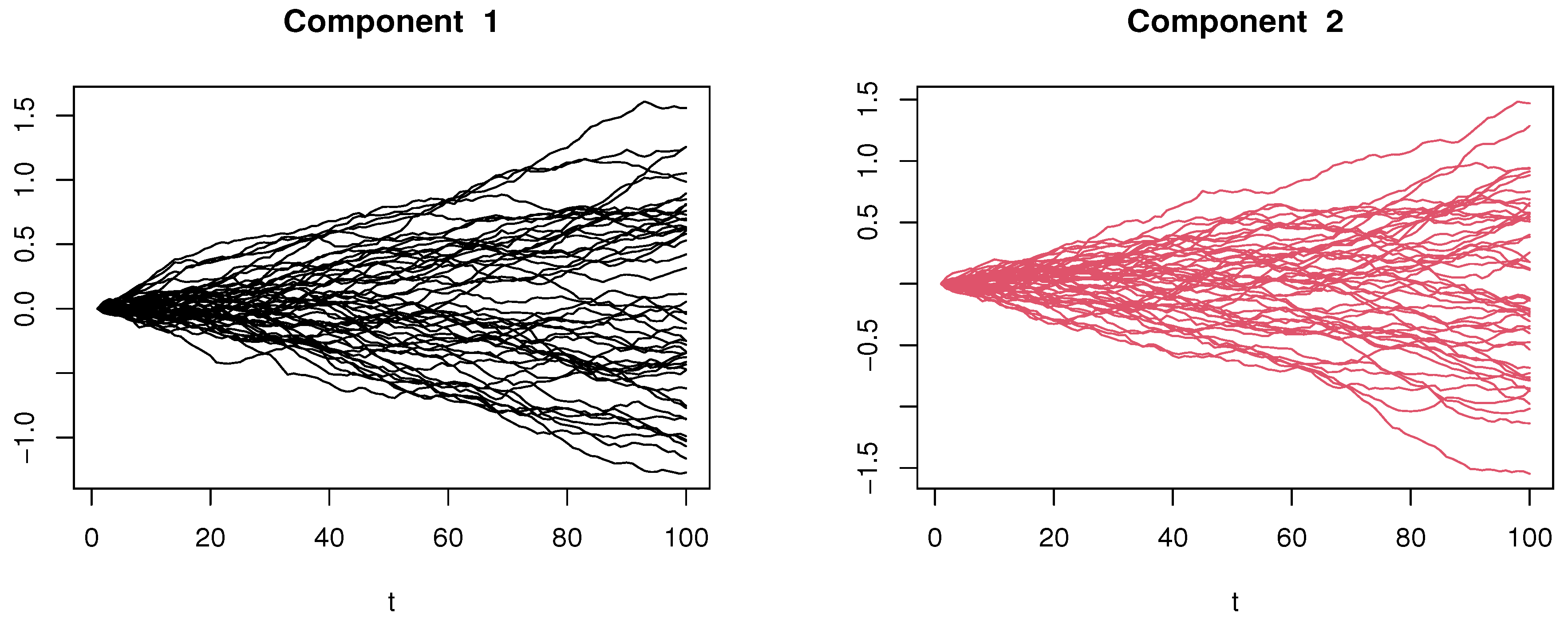
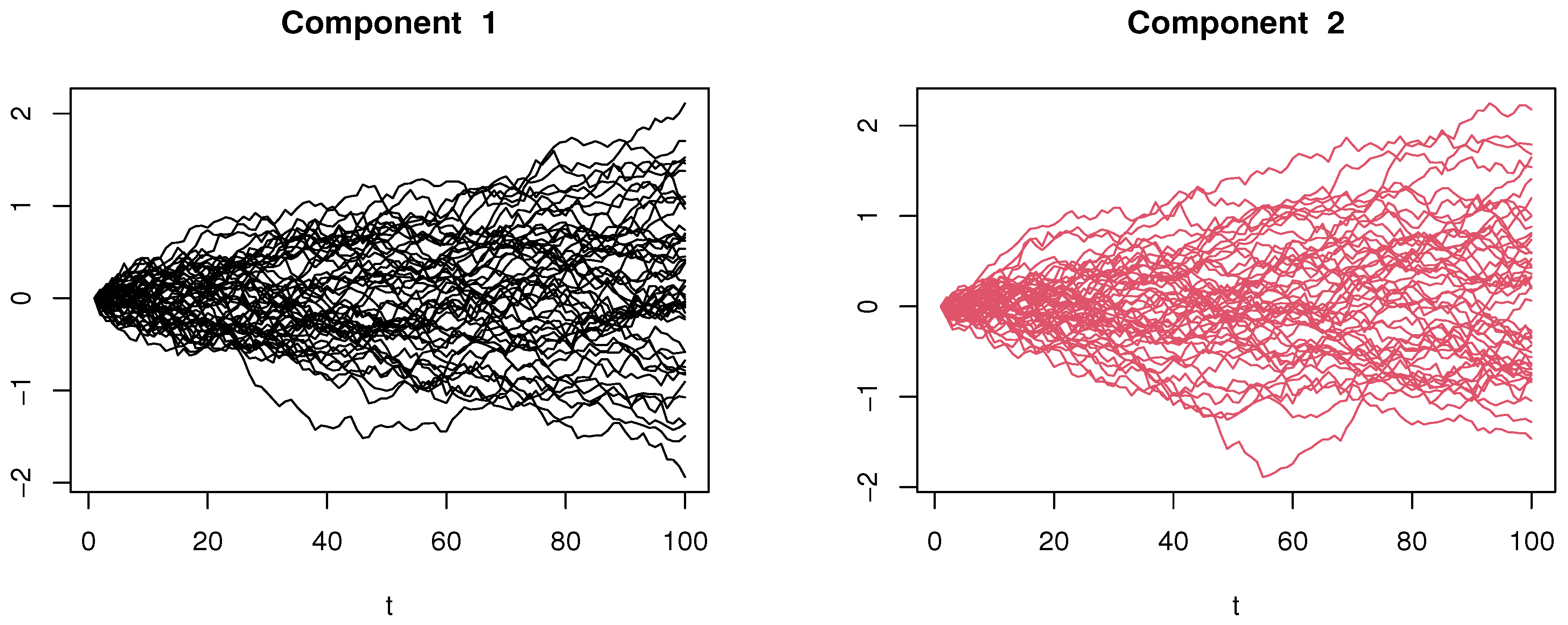
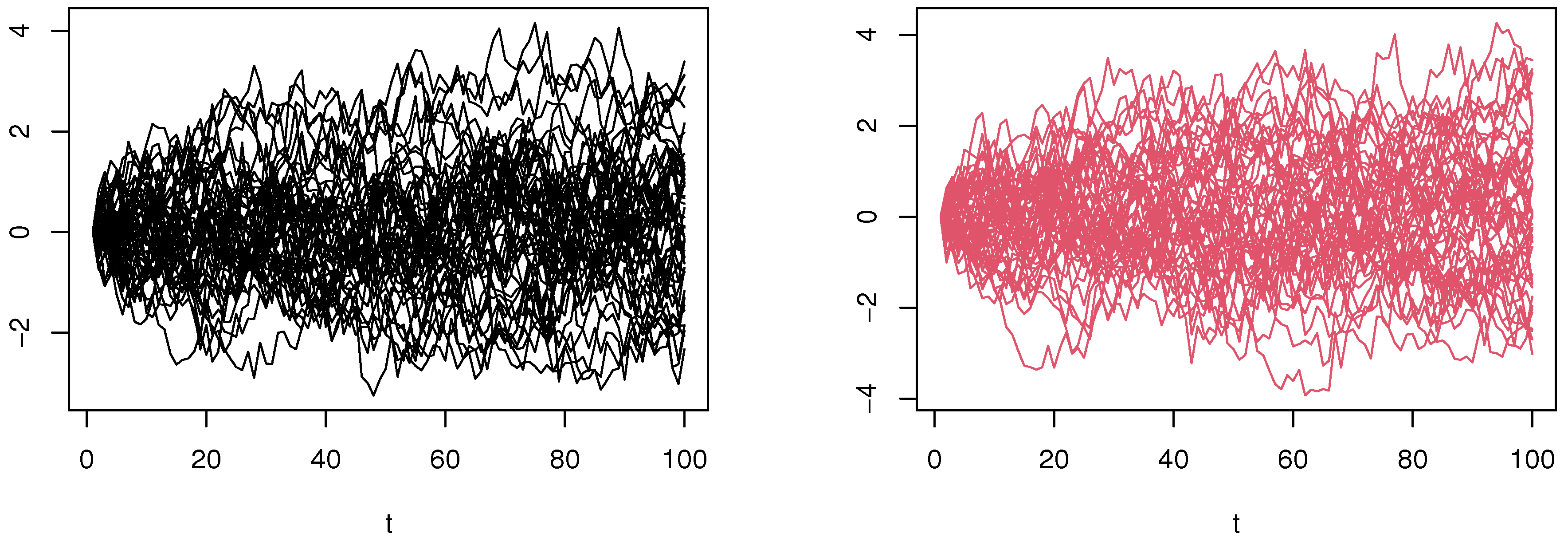
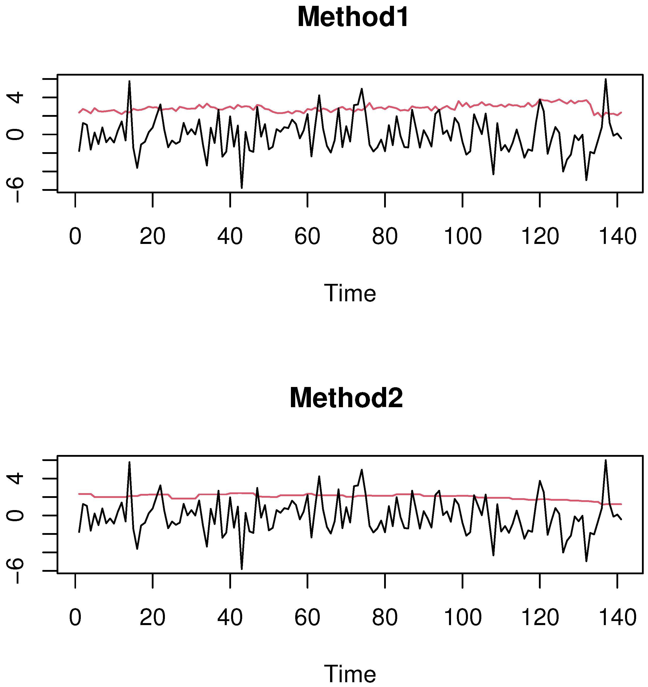
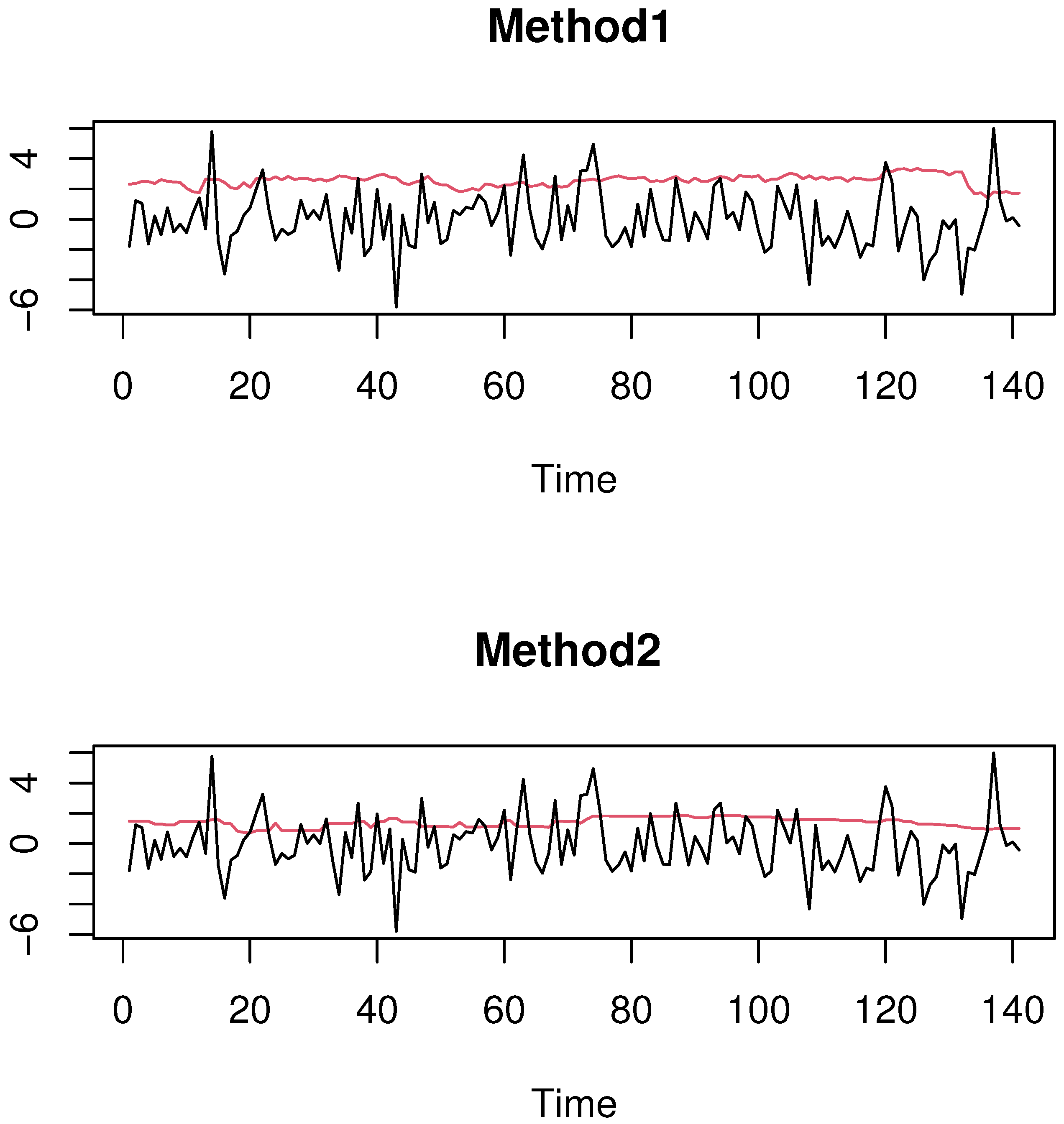
4.1. Simulated Financial Time-Series Analysis

The main purpose of this Section is to evaluate the applicability of the new estimator $\widehat{Q{P}_p}\left(\mathcal{V}\right)$ using simulated financial time series. Therefore, we assume control of the return of portfolio with d financial assets and examine the performance of $\widehat{Q{P}_p}\left(\mathcal{V}\right)$ as risk detector of the average of the daily variation of the d financial assets. For this simulation experiment we draw the functional covariate from sampling process (1). More precisely, we simulate a Volterra process with $d=2$ using the R-package (version is 4.3.1) Sim.DiffProc through the routine code st.int. In this routine code we employ the fractional kernel with h defined by

$$\mathcal{L}(t,s)={(t-s)}^{h-0.5}.$$

The different components of the multi-functional explanatory variables ${\mathcal{C}}_k\left(s\right)$ are plotted in the following Figure 1, Figure 2 and Figure 3.

As mentioned below, the interest variables ${\mathcal{S}}_k$ are chosen as the average of the variation of the components of the functional variables ${\mathcal{C}}_k\left(s\right)$. We point out that the primary step of the applicability of the estimator $\widehat{Q{P}_p}\left(\mathcal{V}\right)$ lies in the determination of its parameters. In this empirical analysis we use the cross-validation rules used by [15,23]. It selects the smoothing parameter a locally using the k-nearest neighborhood approach as follows:

$$\begin{array}{ccc}\hfill a_{opt}& =& \arg \min {\displaystyle \frac{1}{n}}{\Sigma }_{k=1}^n{\left({\mathcal{S}}_k-\widehat{Q{P}_{0.5}}\left({\mathcal{C}}_k\right)\right)}^2.\hfill \end{array}$$

(13)

where

$$H=\left\{a\ge 0:{\Sigma }_{i=1}^{n}1{\mathrm{I}}_{B(\theta ,a)}\left({\mathcal{C}}_i\right)=k\right\},$$

where $k\in \{5,15,25,\dots ,0.5n\}$. Furthermore, we have simulated by the quadratic kernel on $(0,1)$ and, we have employed the PCA metric which is more adequate for this kind of functional variable input (see the curve shapes in Figure 1, Figure 2 and Figure 3). Finally we examine the feasibility of the estimator $\widehat{Q{P}_p}\left(\right)$ by comparing it to the parametric one obtained by the code routine CVaR R-code in the package PerformanceAnalytics. The performance of both risk models are tested via backtesting using

$$\begin{array}{ccc}\hfill ALS\left(p\right)& =& {\displaystyle \frac{1}{N}}{\Sigma }_{k=1}^N{\rho }_p\left({\mathcal{S}}_k,\widehat{Q{P}_p}\left({\mathcal{C}}_k\right)\right).\hfill \end{array}$$

(14)

where ${\rho }_p\left(t\right)=t^2\left|p-1{\mathrm{I}}_{t\le 0}\right|$.

The results obtained are summarized in

Table 1. The $ALS\left(p\right)$ for different scenarios.

Model	h	N	$\mathit{p}=0.1$	$\mathit{p}=0.05$	$\mathit{p}=0.01$
$\widehat{Q{P}_p}$	0.2	50	1.89	1.76	1.59
		150	1.12	1.02	1.07
		250	0.81	0.64	0.73
	0.6	50	1.57	1.41	1.61
		150	0.96	0.85	0.72
		250	0.31	0.23	0.28
	0.9	50	1.18	1.17	1.23
		150	1.02	1.09	1.11
		250	0.18	0.25	0.33
CVaR	0.2	50	1.19	1.23	1.25
		150	1.07	1.12	1.26
		250	0.97	0.74	0.83
	0.6	50	1.85	1.91	1.71
		150	1.11	1.03	1.12
		250	0.71	0.46	0.53
	0.9	50	2.20	2.21	2.33
		150	2.14	2.19	2.081
		250	1.078	1.05	0.76

, which presents the values of $ALS\left(p\right)$ for different sample sizes ($N=50,150,250$), three probability levels ($p=0.1,0.05,0.01$), and three distinct values of the Hurst parameter values in (0,1) (small, mid, and strong) that are $h=0.2,0.6,0.9$.

The obtained results illustrate the easy implementation of the estimator $\widehat{Q{P}_p}\left(\mathcal{V}\right)$. The behavior of $\widehat{Q{P}_p}\left(\mathcal{V}\right)$ is significantly influenced by the Hurst parameter h, which plays a crucial role in financial time-series analysis. Specifically, it is well-established that the estimation error varies with different values of h. Lower values of h are associated with rough volatility and have errors varying between (0.64, 1.89). Whereas higher values correspond to long-memory processes and give small errors between (0.18, 1.23). This result confirms the trend-reinforcing behavior of the Hurst parameter. Furthermore, the empirical findings demonstrate a strong alignment with the theoretical predictions for $\widehat{Q{P}_p}\left(\mathcal{V}\right)$. In that sense, the performance of the estimator is profoundly affected by the underlying characteristics of the multifractional volatility time-series model (MFVTSM) process.

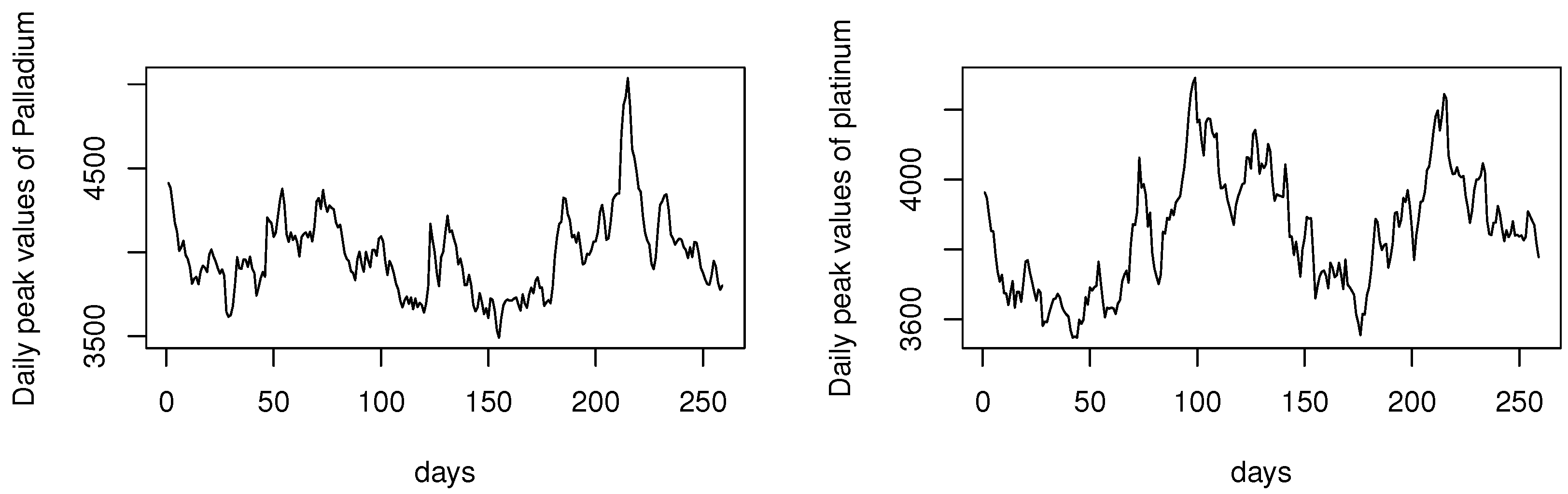
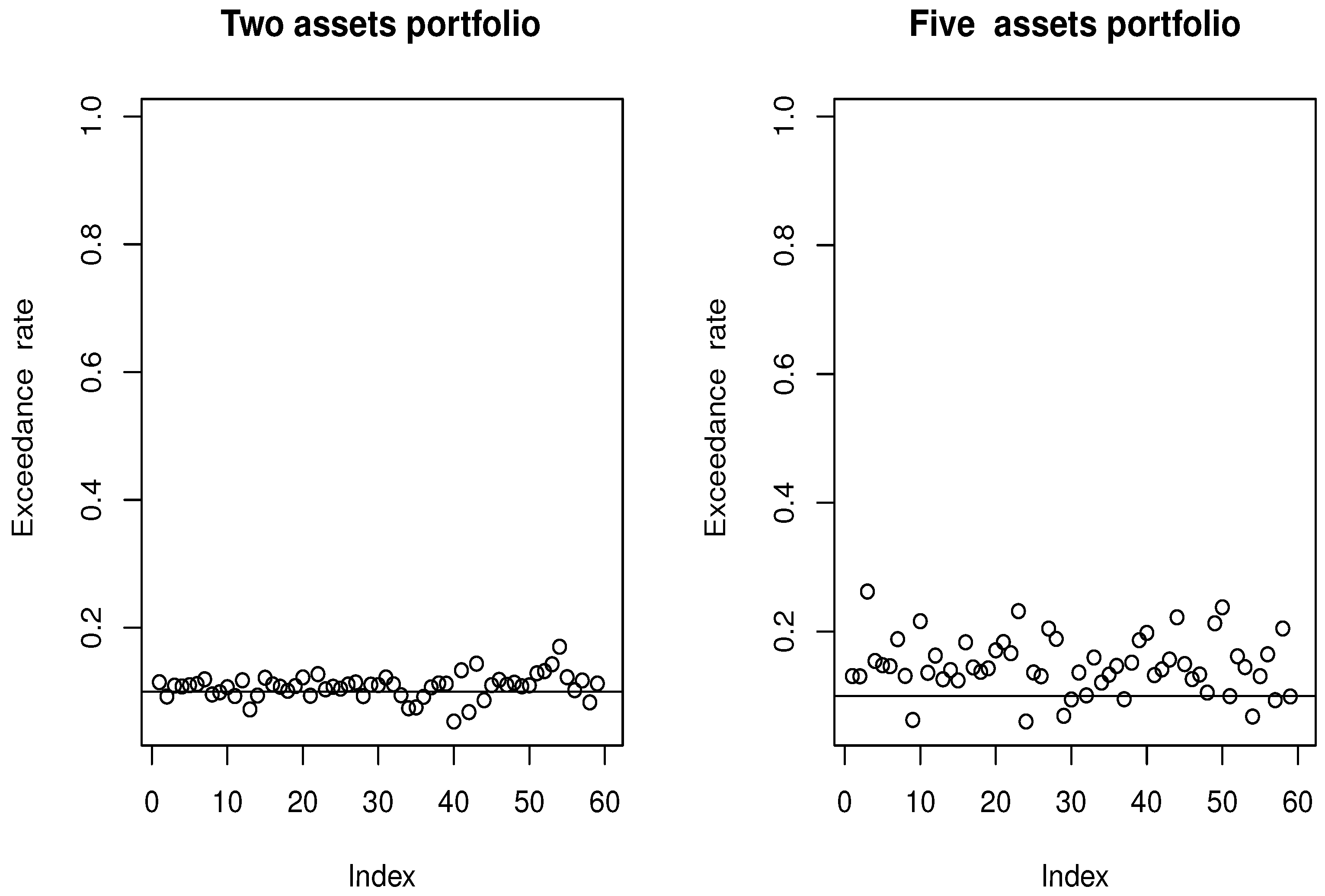
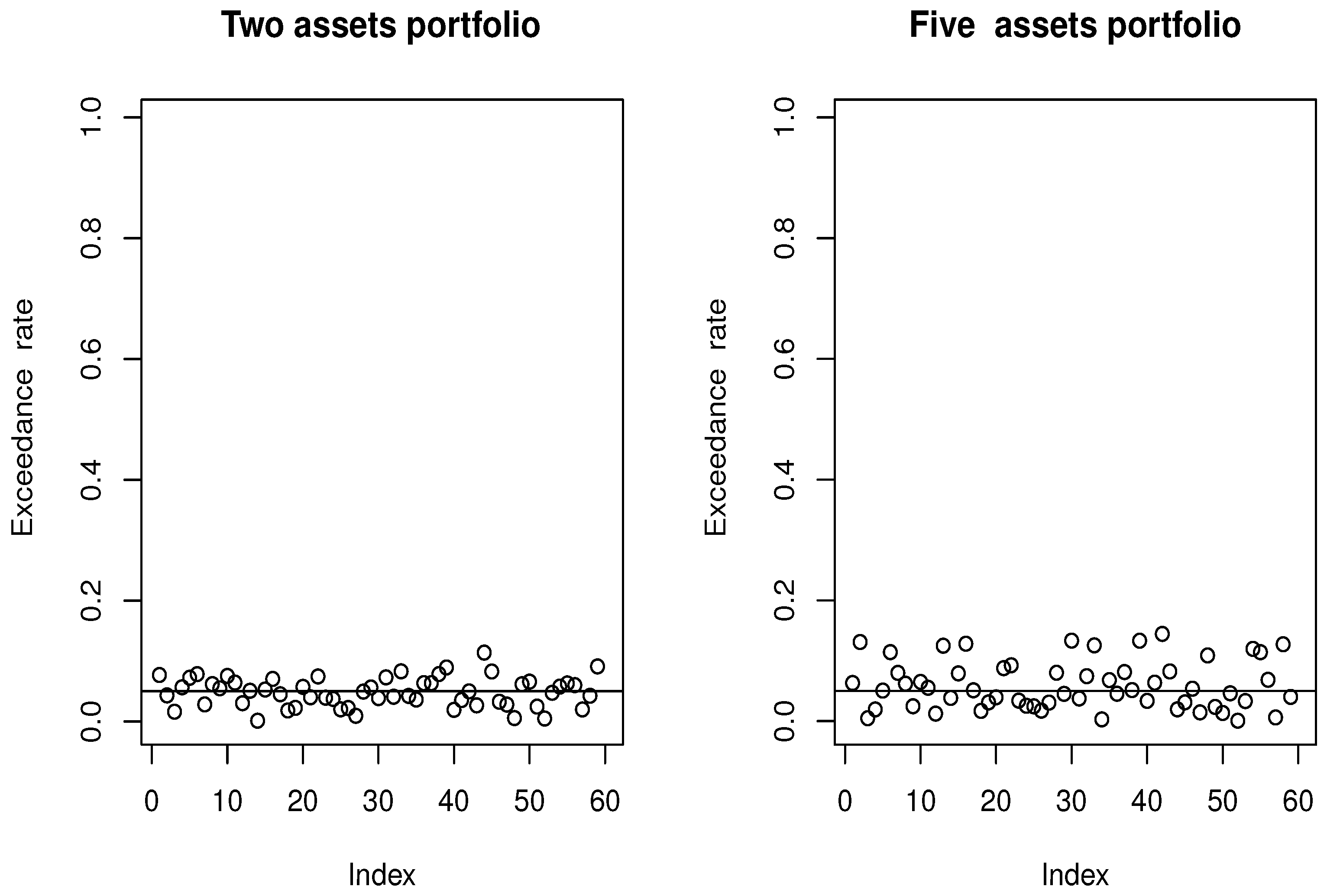
4.2. Real-World Financial Time Series

One of the most challenging issues in financial risk management is determining suitable decision rules that detect the extreme loss or extreme gain. Based on the definition of quantile regression estimation, $\widehat{Q{P}_p}\left(\mathcal{V}\right)$ appears to be a promising solution to this problem. In fact, $\widehat{Q{P}_p}\left(\mathcal{V}\right)$ emphasizes analyzing financial time-series data in a functional nonparametric manner. In particular, functional estimation allows us to incorporate the functional aspects of financial time series. The particularity of this contribution lies in its consideration of multidimensional data, enabling us to assess the risk of multiple assets simultaneously. For this study, we assume that $d=2$ and define ${\mathcal{C}}_k$ as the daily peak values of two precious metals: Platinum (XPT) and Palladium (XPD). The data are available on the website [https://stooq.com/db/h/] (accessed on 28 March 2025). We analyze the daily dynamic of these metals during 2024 (from 1 January 2024 to 31 December 2024). The data for the two metals are displayed in the following (Figure 4).

Usually we are interested in the log-return, defined by

$$z\left(s\right):=100\left(log\left(\mathcal{C}\left(s\right)\right)-log\left(\mathcal{C}(s-1)\right)\right),$$

and we forecast the average variation of the return giving the process $z\left(s\right)$ for $t\in [0,T).$ It is evident that the modified financial time series $z\left(s\right)$ has a zero mean and shows considerable volatility. Before considering this financial time series as functional data, we begin by replicating the Volterra process and create a functional sample using the sampling method mentioned in Section 2.2. We divide $z\left(s\right)$ into $N=220$ curves, each corresponding to one month. While our goal is to predict the $\mathcal{S}$ average of the monthly variations among the two metals, we will then compare the effectiveness of the proposed method against traditional risk measures like $VaR\left(\mathcal{V}\right)$, which is obtained by CVaR R-code in the package PerformanceAnalytics. Furthermore, for the practical determination of $\widehat{Q{P}_p}$, we use the quadratic kernel on $[0,1]$ and the Principal Component Analysis (PCA)-based metric (refer to [15] for its definition). We choose the optimal smoothing parameter a through the local k-nearest neighborhood approach using the same rule as the previous section. We compare both estimators by plotting in Figure 5 and Figure 6 the two estimators $\widehat{Q{P}_p}$ (Method 1) and CVaR (Method 2) and (the curves in red) compared to the true values of the process of the last three months. This reveals violation cases when the process $\mathcal{S}\left(t\right)$ exceeds the estimators.

The obtained results demonstrate that Method 1 ($\widehat{Q{P}_p}$) performs better in detecting the financial risk than its competitor, Method 2 (CVaR). This conclusion is confirmed by the frequency of exceedance (represented by the red curves), which remains consistently closer to the nominal threshold p. More precisely, we examine the percentage of cases where the true curve is superior to $\widehat{\theta }\left(t\right)$, with $\widehat{\theta }$ representing either (CVaR) or $\widehat{Q{P}_p}$. For $p=0.1$, the exceedance rate is approximately 0.12 for $\widehat{Q{P}_p}$ compared to 0.18 for CVaR. Similarly, when $p=0.05$, the observed rates are 0.049 for $\widehat{Q{P}_p}$ versus 0.058 for (CVaR). These results consistently favor Method 1 across different threshold levels.

In the second illustration we examine the impact of the number of assets on the accuracy of $\widehat{Q{P}_p}$ to detect the financial risk. For this second purpose, we consider the daily price of a portfolio that contains high values of a certain number of crypto-currencies such as, Bitcoin, Biconomy, Binance, BinaryX, and Bora. The data are available on the same website https://stooq.com/db/h/ (accessed on 8 June 2025). It is clear that this portfolio contains assets from different platforms. Typically, Bitcoin is the first and most accessible digital currency, characterized by its rapid expansion and high volatility, while Biconomy cryptocurrency is based on simplifying Web3 interactions and cross-chain transfers. Binance Coin is a prominent cryptocurrency initially launched by the Binance exchange in 2017. BinaryX (BNX) is a cryptocurrency platform known for its unpredictable price, with increases and decreases which defy general market trends. Finally, BORA is a cryptocurrency associated with the BORA platform that utilizes Ethereum blockchain to enhance transactions. The feasibility of the model $\widehat{Q{P}_p}$ is assessed by computing the percentage of exceedance points relative to the estimated quantity $\widehat{Q{P}_p}$. To ensure robustness, we repeatedly split the dataset into learning and testing subsets. From a technical point of view, this backtesting measure helps investors to assess the reliability of their risk models under conditions of market volatility. Specifically, we repeat the splitting process between learning and testing sample (60 times) and we calculate the exceedance rate. Figure 7 and Figure 8 present the computational results obtained for two distinct probability thresholds ($p=0.1$ and $p=0.05$), considering two portfolio configurations: a five-asset portfolio and a specialized portfolio comprising Bitcoin and Biconomy.

Without surprise, the accuracy of risk estimation exhibits a strong dependence on the number of components in the multi-functional vector time-series models (MFVTSM). More precisely, the precision of the estimator $\widehat{Q{P}_p}$ deteriorates as the portfolio size increases. This relationship is quantitatively verified through the computation of the Average Exceedance Percentage (AEP). Our empirical analysis reveals that for a probability threshold of $p=0.1$, the AEP increases from approximately 0.13 for portfolios containing two assets to 0.18 for portfolios comprising five assets. Similarly, when considering a more stringent threshold of $p=0.05$, we observe an AEP of 0.049 for two-asset portfolios compared to 0.067 for five-asset portfolios. These findings highlight the significant impact of the dimensionality parameter d (representing the number of components of regressors or the number of assets in the portfolio) on the performance of MFVTSM models.

5. Conclusions

Pushed by the necessity to create a modern algorithm for instant financial risk management, we have introduced innovative statistical methods for high-frequency data observed every minute. This novel approach serves as an alternative to traditional models, specifically those based on the multivariate GARCH model. Our proposed methods offer more insightful information than the conventional model. This is primarily because the multivariate GARCH model relies on specific assumptions about data distribution that are typically unmet, and fails to recognize high-frequency data. Recall that, with advances in technology, digital financial risk management is becoming essential, necessitating the modernization of traditional models. In this context our empirical analysis has shown that the multi-functional VaR model outperforms the common approach. Despite the significant practical impact of these results, they also pave the way for future developments. For instance, comparing semiparametric estimations with nonparametric functional techniques will be crucial moving forward, notably partial linear estimation using similar techniques to quantile regression. In particular, the partial linear estimation is a good alternative allowing the user to enhance the accuracy and the robustness of quantile regression by combining parametric and nonparametric components. It would also be beneficial to explore alternative estimators for quantile regression using a knn approach or treating more complicated structures.

References

1. Comte, F.; Renault, E. Long memory in continuous-time stochastic volatility models. Math. Financ. 1998, 8, 291–323. [Google Scholar] [CrossRef]
2. Alòs, E.; León, J.A.; Vives, J. On the short-time behavior of the implied volatility for jump-diffusion models with stochastic volatility. Financ. Stoch. 2007, 11, 571–589. [Google Scholar] [CrossRef]
3. Fouque, J.P.; Papanicolaou, G.; Sircar, K.R. Derivatives in Financial Markets with Stochastic Volatility; Cambridge University Press: Cambridge, UK, 2000. [Google Scholar]
4. Tankov, P. Financial Modelling with Jump Processes; Chapman and Hall/CRC: Boca Raton, FL, USA, 2003. [Google Scholar]
5. Engle, R.F.; Manganelli, S. CAViaR: Conditional autoregressive value at risk by regression quantiles. J. Bus. Econ. Stat. 2004, 22, 367–381. [Google Scholar] [CrossRef]
6. Kuester, K.; Mittnik, S.; Paolella, M.S. Value-at-risk prediction: A comparison of alternative strategies. J. Financ. Econ. 2006, 4, 53–89. [Google Scholar] [CrossRef]
7. Sun, P.; Lin, F.; Xu, H.; Yu, K. Estimation of value-at-risk by Lp quantile regression. Ann. Inst. Stat. Math. 2025, 77, 25–59. [Google Scholar] [CrossRef]
8. Lux, M.; Härdle, W.K.; Lessmann, S. Data driven value-at-risk forecasting using a SVR-GARCH-KDE hybrid. Comput. Stat. 2020, 35, 947–981. [Google Scholar] [CrossRef]
9. Herrera, R.; Schipp, B. Value at risk forecasts by extreme value models in a conditional duration framework. J. Empir. Financ. 2013, 23, 33–47. [Google Scholar] [CrossRef]
10. Huang, J.-J.; Lee, K.-J.; Liang, H.; Lin, W.-F. Estimating value at risk of portfolio by conditional copula-GARCH method. Insur. Math. Econ. 2009, 45, 315–324. [Google Scholar] [CrossRef]
11. Stone, C.J. Consistent Nonparametric Regression. Ann. Statist. 1977, 5, 595–620. [Google Scholar] [CrossRef]
12. Stute, W. Conditional empirical processes. Ann. Statist. 1986, 14, 638–647. [Google Scholar] [CrossRef]
13. Koenker, R. Quantile regression: 40 years on. Annu. Rev. Econ. 2017, 9, 155–176. [Google Scholar] [CrossRef]
14. Cardot, H.; Crambes, C.; Sarda, P. Quantile regression when the covariates are functions. J. Nonparametric Stat. 2005, 17, 841–856. [Google Scholar] [CrossRef]
15. Ferraty, F.; Vieu, P. Nonparametric Functional Data Analysis: Theory and Practice; Springer Series in Statistics; Springer: New York, NY, USA, 2006. [Google Scholar]
16. Messaci, F.; Nemouchi, N.; Ouassou, I.; Rachdi, M. Local polynomial modelling of the conditional quantile for functional data. Stat. Methods Appl. 2015, 24, 597–622. [Google Scholar] [CrossRef]
17. Ling, N.; Yang, Y.; Peng, Q. Partial linear quantile regression model with incompletely observed functional covariates. J. Nonparametric Stat. 2025, 1–27. [Google Scholar] [CrossRef]
18. Mutis, M.; Beyaztas, U.; Karaman, F.; Lin Shang, H. On function-on-function linear quantile regression. J. Appl. Stat. 2025, 52, 814–840. [Google Scholar] [CrossRef] [PubMed]
19. Beyaztas, U.; Tez, M.; Shang, H.L. Robust scalar-on-function partial quantile regression. J. Appl. Stat. 2024, 51, 1359–1377. [Google Scholar] [CrossRef] [PubMed]
20. Agarwal, G.; Sun, Y. Bivariate Functional Quantile Envelopes with Application to Radiosonde Wind Data. Technometrics 2020, 63, 199–211. [Google Scholar] [CrossRef]
21. Lim, K.P.; Brooks, R.D.; Kim, J.H. Financial crisis and stock market efficiency: Empirical evidence from Asian countries. Int. Rev. Financial Anal. 2008, 17, 571–591. [Google Scholar] [CrossRef]
22. Laksaci, A.; Lemdani, M.; Ould-Saïd, E. A generalized L1-approach for a kernel estimator of conditional quantile with functional regressors: Consistency and asymptotic normality. Stat. Probab. Lett. 2009, 79, 1065–1073. [Google Scholar] [CrossRef]
23. Rachdi, M.; Vieu, P. Nonparametric regression for functional data: Automatic smoothing parameter selection. J. Stat. Plan. Inference 2007, 137, 2784–2801. [Google Scholar] [CrossRef]
24. Alkhaldi, S.H.; Alshahrani, F.; Alaoui, M.K.; Laksaci, A.; Rachdi, M. Multifunctional Expectile Regression Estimation in Volterra Time Series: Application to Financial Risk Management. Axioms 2025, 14, 147. [Google Scholar] [CrossRef]
25. Doukhan, P.; Neumann, M.H. Probability and moment inequalities for sums of weakly dependent random variables, with applications. Stoch. Process. Their Appl. 2007, 117, 878–903. [Google Scholar] [CrossRef]
Figure 1. The components of the case h = 0.9.
Symmetry 17 01207 g001
Figure 2. The components of the case h = 0.6.
Symmetry 17 01207 g002
Figure 3. The components of the case h = 0.2.
Symmetry 17 01207 g003
Figure 4. The two components of the functional regressor C .
Symmetry 17 01207 g004
Figure 5. Comparison between Q P p ^ and CVaR: Case p = 0.05 .
Symmetry 17 01207 g005
Figure 6. Comparison between Q P p ^ and CVaR: Case p = 0.1 .
Symmetry 17 01207 g006
Figure 7. Comparison of the exceedance rate: Case p = 0.1 highlighted by the black line.
Symmetry 17 01207 g007
Figure 8. Comparison of the exceedance rate: Case p = 0.05 highlighted by the black line.
Symmetry 17 01207 g008