A K-Means Clustering Algorithm with Total Bregman Divergence for Point Cloud Denoising

Abstract

Point cloud denoising is essential for improving 3D data quality, yet traditional K-means methods relying on Euclidean distance struggle with non-uniform noise. This paper proposes a K-means algorithm leveraging Total Bregman Divergence (TBD) to better model geometric structures on manifolds, enhancing robustness against noise. Specifically, TBDs—Total Logarithm, Exponential, and Inverse Divergences—are defined on symmetric positive-definite matrices, each tailored to capture distinct local geometries. Theoretical analysis demonstrates the bounded sensitivity of TBD-induced means to outliers via influence functions, while anisotropy indices quantify structural variations. Numerical experiments validate the method’s superiority over Euclidean-based approaches, showing effective noise separation and improved stability. This work bridges geometric insights with practical clustering, offering a robust framework for point cloud preprocessing in vision and robotics applications.

1. Introduction

In recent years, the rapid advancement of 3D scanning technologies has led to an explosion of point cloud data in various fields, including computer vision, robotics, and autonomous systems [1,2,3,4]. As raw digitalizations of physical structures, point clouds often contain inherent noise that degrades segmentation and 3D reconstruction fidelity. Despite their utility, raw point cloud datasets frequently contain inherent imperfections like noise and outliers that compromise the accuracy of downstream applications including segmentation and 3D reconstruction. This inherent data quality challenge necessitates robust denoising algorithms as a fundamental preprocessing requirement for reliable 3D analysis [5,6,7,8,9,10].

Among the various denoising techniques, clustering-based methods have shown promising results due to their ability to group similar points together and distinguish between signal and noise [11,12]. While conventional K-means clustering demonstrates effectiveness in regular data spaces, its dependence on isotropic distance measures creates fundamental limitations when processing irregular 3D structures. Specifically, the Euclidean metric fails to adequately characterize manifold geometries inherent to point cloud data, particularly under spatially variant noise conditions.

Our methodological contribution resolves this through a density-aware clustering framework that adapts to local topological characteristics [13,14]. Given the differences in local geometric structures between noise and valid data on the manifold, points with similar local features should be grouped together into the same cluster. Previous studies [15,16] have employed the K-means clustering algorithm for point cloud denoising, but they relied solely on a limited number of metrics to measure distances on the manifold. Furthermore, these studies overlooked the influence function, which is crucial for evaluating the robustness of the mean derived from each metric in the presence of outliers.

Conversely, [17] proposed a point cloud denoising method leveraging the geometric structure of the Gaussian distribution manifold, employing five distinct measures: Euclidean distance, Affine-Invariant Riemannian Metric (AIRM), Log-Euclidean Metric (LEM), Kullback–Leibler Divergence (KLD), and its symmetric variant (SKLD). The research evaluated metric robustness by deriving influence functions for mean estimators under outlier conditions. Experimental results revealed that geometric metrics outperformed Euclidean measurements in denoising quality, with geometric means showing greater outlier resistance than arithmetic means. Notably, KLD and SKLD demonstrated computational advantages over AIRM/LEM through reduced complexity.

However, [17] had three key limitations: Lack of theoretical bounds for influence functions, high computational complexity ($O\left(n^4\right)$) from iterative mean calculations, and absence of quantitative measures for local geometric variations.

More recently, Xu et al. [10] introduced TDNet, a deep learning approach achieving state-of-the-art results but requiring substantial GPU resources that limit real-time applications. Parallel developments in Bregman divergences show promising theoretical properties yet remain underexplored for 3D data: Liu et al. [18] established Total Bregman Divergence (TBD) for shape retrieval tasks, while Hua et al. [19] adapted TBD for radar detection without extending it to 3D point processing. To our knowledge, this work presents the first unified framework that integrates TBD with K-means clustering for manifold-aware point cloud denoising, bridging geometric robustness with computational efficiency. To address these gaps, we introduce Total Bregman Divergence (TBD), a novel divergence class that measures orthogonal deviation between a convex differentiable function’s value at one point and its tangent approximation at another. As shown in [18], TBD’s orthogonal projection property offers fundamental advantages over [17]’s framework. These include closed-form mean solutions that avoid iterative optimization (Section 2.2), anisotropy indices for quantifying local geometric distortions (Section 4.1), and bounded influence functions supported by strict theoretical guarantees (Section 4.2).

Building on [17], our TBD-K-means framework provides three fundamental breakthroughs:

• The TBD framework introduces closed-form mean solutions derived through orthogonal projection. This fundamental innovation eliminates the need for iterative optimization in mean estimation procedures.
• Our method establishes theoretically bounded influence functions with strict mathematical guarantees. These bounded functions provide inherent robustness against outliers and data perturbations.
• TBD develops novel anisotropy indices for quantifying local geometric distortions. These indices enable precise characterization of manifold structures in complex data spaces.

This paper is structured into six main sections. Section 1 introduces the importance of point cloud denoising and highlights the limitations of traditional K-means clustering approaches based on Euclidean distance. Section 2 delves into the theoretical foundations, defining TBD and deriving the means of several positive-definite matrices. Section 3 proposes a novel K-means clustering algorithm that leverages TBD for point cloud denoising. Section 4 provides an in-depth analysis of the anisotropy indices of Bregman divergence and the influence functions of the TBD means. Section 5 presents simulation results and performance comparisons, demonstrating the effectiveness of the proposed algorithm. Section 6 concludes by summarizing the main contributions and discussing potential applications and future research directions.

2. Geometry on the Manifold of Symmetric Positive-Definite Matrices

The collection of $n\times n$ real matrices is represented by $M_{n\times n}$, whereas the subset comprising all invertible $n\times n$ real matrices forms the general linear group, denoted as $\mathrm{GL}(n,\mathbb{R})$. Notably, $\mathrm{GL}(n,\mathbb{R})$ possesses a differentiable manifold structure, with $M_{n\times n}$ functioning as its Lie algebra, denoted as $\mathrm{gl}(n,\mathbb{R})$. The exchange of information between $\mathrm{GL}(n,\mathbb{R})$ and $M_{n\times n}$ is facilitated by exponential and logarithmic mappings. In particular, the exponential map, given by

$$\mathrm{Exp}\left(X\right)=\sum _{k=0}^{\infty }{\displaystyle \frac{X^k}{k!}},$$

converts a matrix X in $M_{n\times n}$ to an element in $\mathrm{GL}(n,\mathbb{R})$. Conversely, for an invertible matrix A devoid of eigenvalues on the closed negative real axis, there exists a unique logarithm with eigenvalues within the strip $\{z\in \mathbb{C}|-\pi <\mathrm{Im}\left(z\right)<\pi \}$. This logarithm, serving as the inverse of the exponential map, is termed the principal logarithm map and symbolized by

$$\mathrm{Log}\left(A\right).$$

Let ${\mathcal{S}}_n$ denote the space of real symmetric $n\times n$ matrices:

$${\mathcal{S}}_n=\{X\in {\mathbb{R}}^{n\times n}\mid X=X^T\}.$$

(1)

The subset of symmetric positive-definite matrices (SPD) forms the Riemannian manifold:

$${\mathcal{P}}_n=\{\mathsf{\Sigma }\in {\mathcal{S}}_n\mid {\mathbf{v}}^T\mathsf{\Sigma }\mathbf{v}>0,\forall \mathbf{v}\in {\mathbb{R}}^n\setminus \left\{\mathbf{0}\right\}\}.$$

(2)

Three fundamental metric structures on ${\mathcal{P}}_n$ are considered:

(i)

Euclidean (Frobenius) Framework: The canonical inner product on ${\mathcal{P}}_n$ is defined as

$$\langle X,Y\rangle =\mathrm{tr}\left(X^{T}Y\right),$$

(3)

inducing the norm $\parallel X\parallel =\sqrt{\langle X,X\rangle }$ and metric distance

$$d_F({\mathsf{\Sigma }}_1,{\mathsf{\Sigma }}_2)=\parallel {\mathsf{\Sigma }}_1-{\mathsf{\Sigma }}_2\parallel .$$

(4)

The tangent space $T_{\mathsf{\Sigma }}{\mathcal{P}}_n$ at any $\mathsf{\Sigma }\in {\mathcal{P}}_n$ coincides with ${\mathcal{S}}_n$ due to ${\mathcal{P}}_n$’s open submanifold structure in ${\mathcal{S}}_n$.

(ii)

Affine-Invariant Riemannian Metric (AIRM): The geometry metric at $\mathsf{\Sigma }\in {\mathcal{P}}_n$ is given as follows:

$$g_{\mathsf{\Sigma }}(V,W)=\mathrm{tr}\left({\mathsf{\Sigma }}^{-1}V{\mathsf{\Sigma }}^{-1}W\right),V,W\in T_{\mathsf{\Sigma }}{\mathcal{P}}_n.$$

(5)

This induces the geodesic distance [20,21]:

$$d_{\mathrm{AIRM}}({\mathsf{\Sigma }}_1,{\mathsf{\Sigma }}_2)=\parallel \left({\mathsf{\Sigma }}_1^{-1/2}{\mathsf{\Sigma }}_2{\mathsf{\Sigma }}_1^{-1/2}\right)\parallel .$$

(6)

(iii)

Log-Euclidean Metric (LEM): Through the logarithmic group operation

$${\mathsf{\Sigma }}_1⊛{\mathsf{\Sigma }}_2:=\mathrm{Exp}(\mathrm{Log}\left({\mathsf{\Sigma }}_1\right)+\mathrm{Log}\left({\mathsf{\Sigma }}_2\right)),$$

(7)

${\mathcal{P}}_n$ becomes a Lie group. The metric at $\mathsf{\Sigma }$ is defined via differential mappings:

$$g_{\mathsf{\Sigma }}(V,W)=\langle D_{\mathsf{\Sigma }}\mathrm{Log}\left(V\right),D_{\mathsf{\Sigma }}\mathrm{Log}\left(W\right)\rangle ,$$

(8)

where $D_{\mathsf{\Sigma }}\mathrm{Log}$ denotes the differential of the matrix logarithm. The corresponding distance becomes

$$d_{\mathrm{LEM}}({\mathsf{\Sigma }}_1,{\mathsf{\Sigma }}_2)=\parallel \mathrm{Log}\left({\mathsf{\Sigma }}_1\right)-\mathrm{Log}\left({\mathsf{\Sigma }}_2\right)\parallel ,$$

(9)

effectively Euclideanizing the manifold geometry through logarithmic coordinates.

2.1. Bregman Divergence on Manifold ${\mathcal{P}}_n$

For matrices $A,B\in \mathrm{GL}(n,\mathbb{R})$, the Bregman matrix divergence associated with a strictly convex differentiable potential function $\mathsf{\Phi }$ is given by:

$${\mathcal{D}}_{\mathsf{\Phi }}(A,B)=\mathsf{\Phi }\left(A\right)-\mathsf{\Phi }\left(B\right)-\langle \nabla \mathsf{\Phi }\left(B\right),A-B\rangle ,$$

(10)

where $\langle ·,·\rangle$ denotes the Frobenius inner product [22].

This divergence can be systematically extended to a Total Bregman Divergence (TBD) through the subsequent formulation. For invertible matrices $A,B\in \mathrm{GL}(n,\mathbb{R})$, the TBD is defined as follows [23]:

$${\delta }_{\mathsf{\Phi }}(A,B)={\displaystyle \frac{\mathsf{\Phi }\left(A\right)-\mathsf{\Phi }\left(B\right)-\langle \nabla \mathsf{\Phi }\left(B\right),A-B\rangle }{\sqrt{1+{\parallel \nabla \mathsf{\Phi }\left(B\right)\parallel }^2}}}.$$

(11)

When calculating the divergence associated with a certain convex function $\mathsf{\Phi }\left(A\right)$, the Riemannian gradient of $\mathsf{\Phi }\left(A\right)$ is often needed, which can be obtained based on the covariant/directional derivative related to the Riemannian metric as follows:

$$\langle \nabla \mathsf{\Phi }\left(A\right),X\rangle ={\displaystyle \frac{\mathrm{d}}{\mathrm{d}\epsilon }}{|}_{\epsilon =0}\mathsf{\Phi }\left(\gamma \left(\epsilon \right)\right),\forall X\in T_A{\mathcal{P}}_n$$

(12)

with the curve $\gamma :[0,1]\to {\mathcal{P}}_n$ and $\gamma \left(0\right)=A,\dot{\gamma }\left(0\right)=X$. After linearizing the curve $\gamma$, (12) can be rewritten as follows:

$$\langle \nabla \mathsf{\Phi }\left(A\right),X\rangle ={\displaystyle \frac{\mathrm{d}}{\mathrm{d}\epsilon }}{|}_{\epsilon =0}\mathsf{\Phi }(A+\epsilon X),\forall X\in T_A{\mathcal{P}}_n.$$

(13)

Proposition 1. 

For any nonsingular matrix $A\in \mathrm{GL}(n,\mathbb{R})$ with spectral exclusion condition $\sigma \left(A\right)\cap {\mathbb{R}}_{\le 0}=\varnothing$, there exists a well-defined matrix entropy functional:

$$\mathsf{\Phi }\left(A\right)=\mathrm{tr}\left(A\mathrm{Log}\right(A\left)\right),$$

(14)

which generalizes the scalar function $\varphi \left(x\right)=xlnx$ to the matrix setting through trace-theoretic extension [23]. Then, the Riemannian gradient of $\mathsf{\Phi }\left(A\right)$ is as follows:

$$\nabla \mathsf{\Phi }\left(A\right)=\mathrm{Log}\left(A\right)+I.$$

(15)

Furthermore, the logarithm divergence (LD) is expressed as follows:

$$D_{\mathsf{\Phi }}(A,B)=\mathrm{tr}\left(A\left(\mathrm{Log}\right(A)-\mathrm{Log}(B\left)\right)-(A-B)\right),$$

(16)

and the total logarithm divergence (TLD) is provided as follows:

$${\delta }_{\mathsf{\Phi }}(A,B)={\displaystyle \frac{\mathrm{tr}\left(A\left(\mathrm{Log}\right(A)-\mathrm{Log}(B\left)\right)-(A-B)\right)}{\sqrt{{1+\parallel \mathrm{Log}\left(B\right)+I\parallel }^2}}}.$$

(17)

Proof. 

From (13), $\nabla \mathsf{\Phi }\left(B\right)$ is calculated as follows:

$$\begin{array}{ccc}\hfill \langle \nabla \mathsf{\Phi }\left(B\right),V\rangle & =& {\displaystyle \frac{d}{d\epsilon }}{|}_{\epsilon =0}\mathsf{\Phi }(B+\epsilon V)\hfill \\ & =& {\displaystyle \frac{\mathrm{d}}{\mathrm{d}\epsilon }}{|}_{\epsilon =0}\mathrm{tr}\left(\gamma \left(\epsilon \right)\mathrm{Log}\gamma \left(\epsilon \right)\right)\hfill \\ & =& \mathrm{tr}\left(\mathrm{Log}\left(B\right)V\right)-\mathrm{tr}\left(\gamma \left(\epsilon \right){\displaystyle \frac{d}{d\epsilon }}\mathrm{Log}\gamma \left(\epsilon \right)\right){|}_{\epsilon =0},\hfill \end{array}$$

where

$$\gamma \left(\epsilon \right):=B+\epsilon V.$$

(18)

Next, we will calculate the second term of the above expression, namely the differential term. Using Lemmas 3 and 4 in [17], we obtain the following:

$$\begin{array}{ccc}& & \mathrm{tr}\left(\gamma \left(\epsilon \right){\displaystyle \frac{d}{d\epsilon }}\mathrm{Log}\gamma \left(\epsilon \right)\right)\hfill \\ & =& \mathrm{tr}\left({\int }_0^1\gamma \left(\epsilon \right){\left(\left(\gamma \right(\epsilon )-I)t+I\right)}^{-1}{\displaystyle \frac{d\gamma \left(\epsilon \right)}{d\epsilon }}{\left(\left(\gamma \right(\epsilon )-I)t+I\right)}^{-1}dt\right)\hfill \\ & =& \mathrm{tr}\left({\int }_0^1{\left(\left(\gamma \right(\epsilon )-I)t+I\right)}^{-1}\gamma \left(\epsilon \right){\displaystyle \frac{d\gamma \left(\epsilon \right)}{d\epsilon }}{\left(\left(\gamma \right(\epsilon )-I)t+I\right)}^{-1}dt\right)\hfill \\ & =& {\int }_0^1\mathrm{tr}\left({\left(\left(\gamma \right(\epsilon )-I)t+I\right)}^{-2}\gamma \left(\epsilon \right){\displaystyle \frac{d\gamma \left(\epsilon \right)}{d\epsilon }}\right)dt\hfill \\ & =& \mathrm{tr}\left(\gamma {\left(\epsilon \right)}^{-1}\gamma \left(\epsilon \right)V\right)\hfill \\ & =& \mathrm{tr}\left(V\right).\hfill \end{array}$$

Then, we have

$$\langle \nabla \mathsf{\Phi }\left(B\right),V\rangle =\mathrm{tr}\left(\left(\mathrm{Log}\right(B)+I)V\right)=\langle \mathrm{Log}\left(B\right)+I,V\rangle ,$$

(19)

and thus (15) has been proven. Substituting the result into Equation (10), the proof of Equation (16) is complete.    □

Similar to the proof methodology employed in Proposition 1, we can derive Proposition 2 and Proposition 3 through analogous applications.

Proposition 2. 

Consider $\mathsf{\Phi }\left(A\right)=\mathrm{tr}\left(\mathrm{Exp}\right(A\left)\right),$ which is induced from the function $e^x$ [22]. Then, the Riemannian gradient of $\mathsf{\Phi }\left(A\right)$ is as follows:

$$\nabla \mathsf{\Phi }\left(B\right)=\mathrm{Exp}\left(A\right).$$

(20)

Furthermore, the exponential divergence (ED) is expressed as

$$D_{\mathsf{\Phi }}(A,B)=\mathrm{tr}\left(\mathrm{Exp}\left(A\right)-\mathrm{Exp}\left(B\right)-\mathrm{Exp}\left(B\right)(A-B)\right),$$

(21)

and the total exponential divergence (TED) is provided by

$${\delta }_{\mathsf{\Phi }}(A,B)={\displaystyle \frac{\mathrm{tr}\left(\mathrm{Exp}\right(A)-\mathrm{Exp}(B)-\mathrm{Exp}(B\left)\right(A-B\left)\right)}{\sqrt{1+{\parallel \mathrm{Exp}\left(B\right)\parallel }^2}}}.$$

(22)

Proposition 3. 

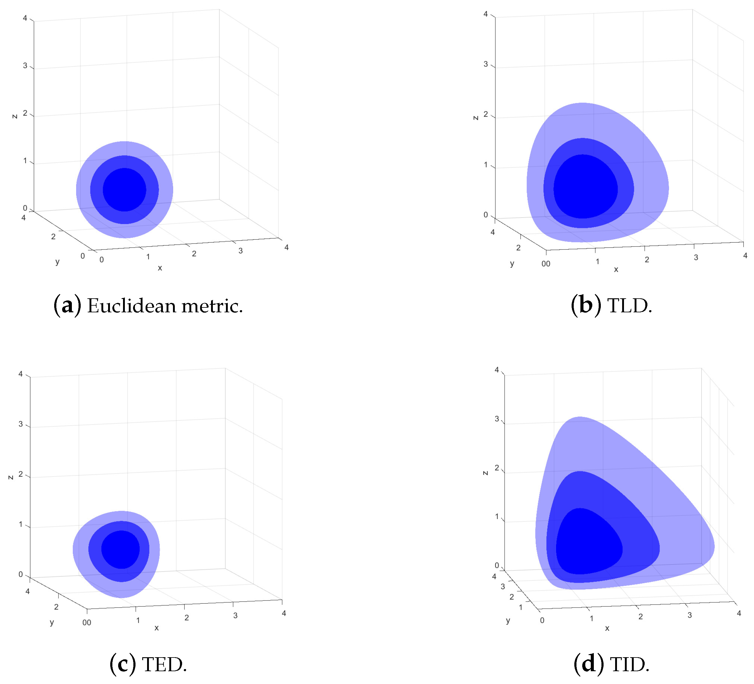
When A is invertible, let $\mathsf{\Phi }\left(A\right)=\mathrm{tr}\left(A^{-1}\right)$, which is induced from the function ${\displaystyle \frac{1}{x}}$ [22]. Then, the Riemannian gradient of $\mathsf{\Phi }\left(A\right)$ is as follows:

$$\nabla \mathsf{\Phi }\left(B\right)=-B^{-2}.$$

(23)

Furthermore, the inverse divergence (ID) is expressed as follows:

$$D_{\mathsf{\Phi }}(A,B)=\mathrm{tr}\left(A^{-1}+A{B}^{-2}-2B^{-1}\right),$$

(24)

and the total inverse divergence (TID) is provided as follows:

$${\delta }_{\mathsf{\Phi }}(A,B)={\displaystyle \frac{\mathrm{tr}\left(A^{-1}+A{B}^{-2}-2B^{-1}\right)}{\sqrt{1+\parallel B^{-2}{\parallel }^2}}}.$$

(25)

To analyze the differences among the TBD divergences defined on the positive-definite matrix manifold, Figure 1 shows three-dimensional isosurfaces centered at the identity matrix, which are induced by TLD, TED, and TID, respectively. All of these isosurfaces are convex balls with non-spherical shapes, differing completely from the spherical isosurfaces in the context of the Euclidean metric.

2.2. TBD Means on ${\mathcal{P}}_n$

In this subsection, we study the geometric mean of several symmetric positive-definite matrices induced by the TBD, by considering the minimization problem of an objective function.

For m positive real numbers $\left\{a_i\right\}$, the arithmetic mean is often denoted as $\widehat{a}$ and expressed as

$$\overline{a}:={\displaystyle \frac{1}{m}}\sum _{i=1}^m{a}_i=arg\underset{a>0}{min}\sum _{i=1}^m{|a-a_i|}^2,$$

(26)

where $|a-a_i|$ represents the absolute difference between a and $a_i$, which signifies the distance separating the two points on the real number line. The mean of m SPD $\{A_1,A_2,\dots ,A_m\}\in {\mathcal{P}}_n$ is the solution to

$$\overline{A}:=arg\underset{A\in {\mathcal{P}}_n}{min}\sum _{i=1}^m{d}^2(A,A_i).$$

(27)

Thus, the arithmetic mean of $\{A_1,A_2,\dots ,A_m\}$ endowed by the Euclidean metric can be represented as follows:

$$\overline{A}={\displaystyle \frac{1}{m}}\sum _{i=1}^m{A}_i.$$

(28)

And, the mean of $\{A_1,A_2,\dots ,A_m\}$ with LEM is as follows [16]:

$$\overline{A}=\mathrm{Exp}\left({\displaystyle \frac{1}{m}}\sum _{i=1}^m\mathrm{Log}\left(A_i\right)\right).$$

(29)

The result indicates that the Log-Euclidean mean has Euclidean characteristics when considered in the logarithmic domain, whereas AIRM’s mean lacks these properties [17].

The concept extends naturally to the TBD mean. For a strictly convex differentiable function $\mathsf{\Phi }$ and matrices $\{A_1,A_2,\dots ,A_m\}$, the TBD mean is defined as follows:

$$\overline{A}:=arg\underset{A\in {\mathcal{P}}_n}{min}\sum _{i=1}^m{\delta }_{\mathsf{\Phi }}(A,A_i).$$

(30)

The strict convexity of $\mathsf{\Phi }\left(A\right)$ ensures the Bregman divergence ${\sum }_{i=1}^m{\delta }_{\mathsf{\Phi }}(A,A_i)$ retains strict convexity in A. Consequently, uniqueness of the TBD mean (30) follows directly from convex optimization principles, provided such a mean exists. To guarantee existence, ${\delta }_{\mathsf{\Phi }}\left(A\right)$ must operate within a compact subset of ${\mathcal{P}}_n$. Compactness ensures adherence to the Weierstrass extreme value theorem, which mandates attainment of minima for continuous functions over closed and bounded domainsconditions inherently satisfied by the convex functional on this Riemannian manifold. Let us define $H\left(A\right)$ as follows:

$$H\left(A\right):={\displaystyle \frac{1}{m}}\sum _{i=1}^m{\delta }_{\mathsf{\Phi }}(A,A_i).$$

(31)

According to (13), the Riemannian gradient of $H\left(A\right)$ can be obtained as follows:

$$\nabla H\left(A\right)={\displaystyle \frac{1}{m}}\sum _{i=1}^m{\displaystyle \frac{\nabla \mathsf{\Phi }\left(A\right)-\nabla \mathsf{\Phi }\left(A_i\right)}{\sqrt{1+{\parallel \nabla \mathsf{\Phi }\left(A_i\right)\parallel }^2}}}.$$

(32)

Then, by solving $\nabla H\left(A\right)=0$, the  TBD mean can be expressed as

$$\nabla \mathsf{\Phi }\left(\overline{A}\right)=\sum _{i=1}^m{\mathsf{\Omega }}_i\mathsf{\Phi }\left(A_i\right)$$

(33)

with the weight

$${\mathsf{\Omega }}_i={\displaystyle \frac{1}{\sqrt{1+\Vert \nabla \mathsf{\Phi }\left(A_i\right){\Vert }^2}}}/\sum _{j=1}^m{\displaystyle \frac{1}{\sqrt{1+\Vert \nabla \mathsf{\Phi }\left(A_j\right){\Vert }^2}}}.$$

(34)

Next, by substituting (15), (20), and (23) into (33), respectively, it is straightforward to get explicit expressions for the means corresponding to TLD, TED, and TID.

Proposition 4. 

The TLD mean of m SPD $\{A_1,A_2,\dots ,A_m\}$ is provided by

$$\overline{A}=\mathrm{Exp}\left(\sum _{i=1}^m{\mathsf{\Omega }}_i\mathrm{Log}\left(A_i\right)\right),$$

(35)

where

$${\mathsf{\Omega }}_i={\displaystyle \frac{1}{\sqrt{1+\Vert \mathrm{Log}\left(A_i\right){+I\Vert }^2}}}/\sum _{j=1}^m{\displaystyle \frac{1}{\sqrt{1+\Vert \mathrm{Log}\left(A_j\right){+I\Vert }^2}}}.$$

(36)

By comparing (29) and (35), it can be seen that the TLD mean is essentially a weighted version of the LEM mean.

Proposition 5. 

The TED mean of m SPD $\{A_1,A_2,\dots ,A_m\}$ is provided by

$$\overline{A}=\mathrm{Log}\left(\sum _{i=1}^m{\mathsf{\Omega }}_i\mathrm{Exp}\left(A_i\right)\right),$$

(37)

where

$${\mathsf{\Omega }}_i={\displaystyle \frac{1}{\sqrt{1+\Vert \mathrm{Exp}\left(A_i\right){\Vert }^2}}}/\sum _{j=1}^m{\displaystyle \frac{1}{\sqrt{1+\Vert \mathrm{Exp}\left(A_j\right){\Vert }^2}}}.$$

(38)

Proposition 6. 

The TID mean of m SPD $\{A_1,A_2,\dots ,A_m\}$ is provided by

$$\overline{A}={\left(\sum _{i=1}^m{\mathsf{\Omega }}_i{A}_i^{-2}\right)}^{-1/2},$$

(39)

where

$${\mathsf{\Omega }}_i={\displaystyle \frac{1}{\sqrt{1+\Vert A_i^{-2}{\Vert }^2}}}/\sum _{j=1}^m{\displaystyle \frac{1}{\sqrt{1+\Vert A_j^{-2}{\Vert }^2}}}.$$

(40)

3. K-Means Clustering Algorithm with TBDs

In the n-dimensional Euclidean space $R^n$, we denote a point cloud of size $\iota$ as follows:

$$\mathcal{B}:=\{{\mathbf{b}}_i\in R^n\mid i=1,\dots ,\iota \}.$$

(41)

For $\forall \mathbf{b}\in \mathcal{B}$, we first identify its local neighborhood $\mathcal{S}\equiv \Delta (\mathbf{b},q)$ using the k-nearest neighbors algorithm. Subsequently, the intrinsic geometry of $\mathcal{S}$ is characterized by computing two statistical descriptors:

1. The centered mean vector:

$$\mu \left(\mathcal{S}\right):=\mathbb{E}\left[\mathcal{S}\right]-\mathbf{b},$$

where $\mathbb{E}[·]$ denotes empirical expectation;

2. The covariance operator:

$$\mathsf{\Sigma }\left(\mathcal{S}\right):=\mathrm{Cov}(\mathcal{S},\mathcal{S})$$

quantifying pairwise positional deviations.

These descriptors induce a parameterization of $\mathcal{S}$ as points on the statistical manifold of n-dimensional Gaussian distributions:

$${\mathcal{S}}_n=\left\{f\mid f(\mathbf{x};\mu ,\mathsf{\Sigma })={\displaystyle \frac{1}{\sqrt{{\left(2\pi \right)}^n}det\left(\mathsf{\Sigma }\right)}}\mathrm{Exp}\left(-{\displaystyle \frac{{(\mathbf{x}-\mu )}^T{\mathsf{\Sigma }}^{-1}(\mathbf{x}-\mu )}{2}}\right)\right\},$$

(42)

where $\mathbf{x}\in R^n$ and f denotes the probability density function. This geometric embedding facilitates subsequent analysis within the framework of information geometry. The point cloud $\mathcal{B}$ undergoes local statistical encoding through operator $\mathsf{{\rm Y}}$, generating its parametric representation $\tilde{\mathcal{B}}:=\mathsf{{\rm Y}}\left(\mathcal{B}\right)\subset {\mathcal{S}}_n$ in symmetric matrix space. This mapped ensemble, termed the statistical parameter point cloud, preserves neighborhood geometry through covariance descriptors while enabling manifold–coordinate analysis.

Due to the topological homeomorphism between ${\mathcal{S}}_n$ and $R^n\times {\mathcal{P}}_n$ [24], the geometric structure on ${\mathcal{S}}_n$ can be induced by assigning metrics on $R^n\times {\mathcal{P}}_n$. Additionally, the distance on ${\mathcal{S}}_n$ is denoted as

$$d(({\mu }_1,{\mathsf{\Sigma }}_1),({\mu }_2,{\mathsf{\Sigma }}_2))=\parallel {\mu }_1-{\mu }_2\parallel +diff({\mathsf{\Sigma }}_1,{\mathsf{\Sigma }}_2),$$

(43)

where $diff$ stands for the difference between ${\mathsf{\Sigma }}_1$ and ${\mathsf{\Sigma }}_2$. The mean of ${({\mu }_i,{\mathsf{\Sigma }}_i)}_1^{\iota }$ on the parameter point cloud $\tilde{\mathcal{B}}$ is denoted as $({\mathbf{c}}_R,{\mathbf{c}}_P)$, where

$${\mathbf{c}}_R={\displaystyle \frac{1}{\iota }}\sum _{i=1}^{\iota }{\mu }_i,{\mathbf{c}}_P=arg\underset{\mathsf{\Sigma }}{min}\sum _{i=1}^{\iota }{d}^2({\mathsf{\Sigma }}_i,\mathsf{\Sigma }).$$

(44)

The definitions of both distance and mean operators on $\tilde{\mathcal{B}}$ are contingent upon the specific metric structure imposed on $\tilde{\mathcal{B}}$. In our proposed algorithm, these fundamental statistical measures will be directly computed through TBDs, which play a crucial role in establishing the geometric framework for subsequent computations.

The intrinsic statistical properties of valid and stochastic noise components exhibit fundamental divergences in their local structural organizations. This statistical separation forms the basis for our implementation of a K-means clustering framework to partition the complete dataset $\tilde{\mathcal{B}}$ into distinct phenomenological categories: structured information carriers and unstructured random perturbations. The formal procedure for this discriminative clustering operation is systematically outlined in Algorithm 1.

Algorithm 1 Signal–Noise Discriminative Clustering Framework

1. Point Cloud Parametrization: Statistically encode $\mathcal{B}$ into $\tilde{\mathcal{B}}\subset {\mathcal{S}}_n$ via covariance descriptors. 2. Applying the K-means Algorithm: Step a:  Barycenters Setup Assign barycenters (cluster centers) for the two clusters as $({{\mathbf{c}}_R^1}^{\left(\mathrm{i}\right)}$, ${{\mathbf{c}}_P^1}^{\left(\mathrm{i}\right)})$ and ${({\mathbf{c}}_R^2}^{\left(\mathrm{i}\right)}$, ${{\mathbf{c}}_P^2}^{\left(\mathrm{i}\right)})$. Step b:  Grouping with K-means Use the K-means algorithm with the TBDs to group the points in the parameter point cloud $\tilde{\mathcal{B}}$ into two clusters based on their proximity to the current barycenters. Step c:  Updating Barycenters Recalculate the barycenters for the two clusters based on the new clustering results, updating them to $({{\mathbf{c}}_R^1}^{(\mathrm{i}+1)}$ $,{{\mathbf{c}}_P^1}^{(\mathrm{i}+1)})$ and $({{\mathbf{c}}_R^2}^{(\mathrm{i}+1)}$$,{{\mathbf{c}}_P^2}^{(\mathrm{i}+1)})$. Step d:  Convergence Check Set a convergence threshold ${ϵ}_0$ and a convergence condition $d\left(\right({{\mathbf{c}}_R^1}^{\left(\mathrm{i}\right)}$$,{{\mathbf{c}}_P^1}^{\left(\mathrm{i}\right)})$$,({{\mathbf{c}}_R^2}^{(\mathrm{i}+1)}$$,{{\mathbf{c}}_P^2}^{(\mathrm{i}+1)}\left)\right)<{ϵ}_0$. Upon satisfying convergence criteria, project the partitioned clusters in $\tilde{\mathcal{B}}$ to $\mathcal{B}$, then finalize the computation with categorical assignments. If the convergence condition is not met, repeat steps b, c, and d.

Assign initial barycenters for the two clusters as $(c_R^{1\left(0\right)},c_P^{1\left(0\right)})$ and $(c_R^{2\left(0\right)},c_P^{2\left(0\right)})$ using statistical descriptors from any two distinct points in the encoded point cloud $\tilde{B}$. Specifically:

$$(c_R^{1\left(0\right)},c_P^{1\left(0\right)})=({\mu }_i,{\mathsf{\Sigma }}_i),(c_R^{2\left(0\right)},c_P^{2\left(0\right)})=({\mu }_j,{\mathsf{\Sigma }}_j)$$

where $i\ne j$ are arbitrary indices.

4. Anisotropy Index and Influence Functions

This section establishes a unified analytical framework for evaluating geometric sensitivity and algorithmic robustness on ${\mathcal{P}}_n$. Section 4.1 introduces the anisotropy index as a key geometric descriptor, formally defining its relationship with fundamental metrics including the Euclidean metric, AIRM, and the Bregman divergences. Through variational optimization, we derive closed-form expressions for these indices, revealing their intrinsic connections to matrix spectral properties. Section 4.2 advances robustness analysis through influence function theory, developing perturbation models for three central tensor means: TLD, TED, and TID. By quantifying sensitivity bounds under outlier contamination, we establish theoretical guarantees for each mean operator.

4.1. Anisotropy Index Related to Various Metrics

The discriminatory capacity of weighted positive definite matrices manifests through their associated anisotropy measures. Defined intrinsically on the matrix manifold ${\mathcal{P}}_n$, the anisotropy index quantifies local geometric distortion relative to isotropic configurations. For $A\in {\mathcal{P}}_n$, the anisotropy measure relative to the Riemannian metric is as follows:

$$\alpha \left(A\right):=\underset{\epsilon >0}{inf}{d}^2(A,\epsilon I).$$

(45)

This index corresponds to the squared minimal projection distance from A to the scalar curvature subspace $\left\{\epsilon I\right|\epsilon \in {\mathbb{R}}^{+}\}$. Larger $\alpha \left(A\right)$ values indicate stronger anisotropic characteristics. For explicit computation, we minimize the metric-specific functional:

$${\varphi }_A\left(\epsilon \right)=d^2(A,\epsilon I),\epsilon >0.$$

(46)

Next, we systematically investigate anisotropy indices induced by three fundamental geometries: the Frobenius metric representing Euclidean structure, AIRM characterizing curved manifold topology, and Bregman divergences rooted in information geometry. This trichotomy reveals how metric selection governs directional sensitivity analysis on ${\mathcal{P}}_n$.

Following Equations (3) and (45), the anisotropy index associated with the Euclidean metric can be derived through direct computation.

Proposition 7. 

The anisotropy index according to Euclidean metric (3) at a point $A\in {\mathcal{P}}_n$ is given by

$$a_F\left(A\right)=\mathrm{tr}{(A-{\epsilon }^{*}I)}^2,$$

(47)

where

$${\epsilon }^{*}={\displaystyle \frac{\mathrm{tr}\left(A\right)}{n}}.$$

(48)

Proposition 8. 

The anisotropy index associated with AIRM at a point $A\in {\mathcal{P}}_n$ is formulated as

$$a_{AIRM}\left(A\right)=\mathrm{tr}\left({\mathrm{Log}}^2\left({\epsilon }^{*}{A}^{-1}\right)\right),$$

(49)

where

$${\epsilon }^{*}=\sqrt[n]{detA}.$$

(50)

Proof. 

Following (6) and (45), we have

$$\begin{array}{cc}\hfill {\varphi }_A\left(\epsilon \right)& =d^2(A,\epsilon I)=\mathrm{tr}\left({\mathrm{Log}}^2\left(\epsilon A^{-1}\right)\right).\hfill \end{array}$$

(51)

Then, differentiating ${\varphi }_A\left(\epsilon \right)$ with respect to $\epsilon$ yields the expression that

$$\begin{array}{cc}\hfill {\varphi }_A^{\prime }\left(\epsilon \right)& =\mathrm{tr}\left(2\mathrm{Log}\left(\epsilon A^{-1}\right){\displaystyle \frac{d}{d\epsilon }}\mathrm{Log}\left(\epsilon A^{-1}\right)\right).\hfill \end{array}$$

(52)

Let

$$\begin{array}{c}\hfill \gamma \left(\epsilon \right)=\epsilon A^{-1}.\end{array}$$

(53)

Applying Lemma 14 and 15 from Reference [19], we derive the following:

$$\begin{array}{cc}\hfill {\varphi }_A^{\prime }\left(\epsilon \right)=& \mathrm{tr}\left(2\mathrm{Log}\left(\gamma \left(\epsilon \right)\right){\displaystyle \frac{d}{d\epsilon }}\mathrm{Log}\left(\gamma \left(\epsilon \right)\right)\right)\hfill \\ \hfill =& 2\mathrm{tr}(\mathrm{Log}\left(\gamma \left(\epsilon \right)\right){\int }_0^1{\left(\left(\gamma \right(\epsilon )-I)s+I\right)}^{-1}\hfill \\ \hfill & \times {\displaystyle \frac{d\gamma \left(\epsilon \right)}{d\epsilon }}{\left(\left(\gamma \right(\epsilon )-I)s+I\right)}^{-1}ds)\hfill \\ \hfill =& 2\mathrm{tr}\left(\gamma {\left(\epsilon \right)}^{-1}\mathrm{Log}\left(\gamma \left(\epsilon \right)A^{-1}\right)\right)\hfill \\ \hfill =& 2\mathrm{tr}\left({\epsilon }^{-1}\mathrm{Log}\left(\epsilon A^{-1}\right)\right).\hfill \end{array}$$

(54)

With the eigenvalue of A denoted as ${\lambda }_1,{\lambda }_2,\dots ,{\lambda }_n$, Equation (54) can be written as follows:

$${\varphi }_A^{\prime }\left(\epsilon \right)={\displaystyle \frac{2}{\epsilon }}\left(nln\epsilon -ln({\lambda }_1{\lambda }_2\dots {\lambda }_n)\right).$$

(55)

By solving ${\varphi }_A^{\prime }\left(\epsilon \right)=0$, the proof of Equation (49) is complete.    □

Proposition 9. 

The anisotropy index according to the Bregman divergence (16) at a point $A\in {\mathcal{P}}_n$ is formulated as

$$a_L\left(A\right)=\mathrm{tr}\left(A\mathrm{Log}\left(A\right)-A\mathrm{Log}\left({\epsilon }^{*}I\right)-(A-{\epsilon }^{*}I)\right),$$

(56)

where

$${\epsilon }^{*}={\displaystyle \frac{\mathrm{tr}\left(A\right)}{n}}.$$

(57)

Proof. 

Via (16) and (45), we have

$${\varphi }_A\left(\epsilon \right)=\mathrm{tr}\left(A\mathrm{Log}\left(A\right)-A\mathrm{Log}\left(\epsilon I\right)-A+\epsilon I\right),$$

(58)

and

$${\varphi }_A^{\prime }\left(\epsilon \right)=\mathrm{tr}(I-{\displaystyle \frac{1}{\epsilon }}A).$$

(59)

By solving ${\varphi }_A^{\prime }\left(\epsilon \right)=0$, the proof of Equation (56) is complete.    □

Proposition 10. 

The anisotropy index according to the Bregman divergence (21) at a point $A\in {\mathcal{P}}_n$ is formulated as

$$a_E\left(A\right)=\mathrm{tr}\left(\mathrm{Exp}\left(A\right)+\mathrm{Exp}\left({\epsilon }^{*}I\right)(({\epsilon }^{*}-1)I-A)\right),$$

(60)

where

$${\epsilon }^{*}={\displaystyle \frac{\mathrm{tr}\left(A\right)}{n}}.$$

(61)

Proof. 

Via (21) and (45), we have

$${\varphi }_A\left(\epsilon \right)=\mathrm{tr}\left(\mathrm{Exp}\left(A\right)+\mathrm{Exp}\left(\epsilon I\right)\left(\right(\epsilon -1)I-A)\right),$$

(62)

and

$${\varphi }_A^{\prime }\left(\epsilon \right)=e^{\epsilon }(n-\mathrm{tr}\left(A\right)).$$

(63)

By solving ${\varphi }_A^{\prime }\left(\epsilon \right)=0$, the proof of Equation (60) is complete.    □

Proposition 11. 

The anisotropy index associated with the Bregman divergence (24) at a point $A\in {\mathcal{P}}_n$ is given by

$$a_I\left(A\right)=\mathrm{tr}\left(A^{-1}+{\epsilon }^{*-2}A\right)-2n{\epsilon }^{*-1},$$

(64)

where

$${\epsilon }^{*}={\displaystyle \frac{\mathrm{tr}\left(A\right)}{n}}.$$

(65)

Proof. 

Via (24) and (45), we have

$${\varphi }_A\left(\epsilon \right)=\mathrm{tr}\left(A^{-1}+{\epsilon }^{-2}A\right)-2n{\epsilon }^{-1},$$

(66)

and

$${\varphi }_A^{\prime }\left(\epsilon \right)=2n{\epsilon }^{-2}-2{\epsilon }^{-3}\mathrm{tr}\left(A\right).$$

(67)

By solving ${\varphi }_A^{\prime }\left(\epsilon \right)=0$, the proof of Equation (64) is complete.    □

4.2. Influence Functions

This subsection develops a robustness analysis framework through influence functions for symmetric positive-definite matrix-valued data. We systematically quantify the susceptibility of the TBD mean estimators under outlier contamination by deriving closed-form expressions of influence functions. Furthermore, we establish operator norm bounds of influence functions, thereby characterizing their stability margins in perturbed manifold learning scenarios.

Let $\overline{A}$ denote the TBDs mean of mSPD $\{A_1,A_2,\dots ,A_m\}.$ Let $\widehat{A}$ denote the mean after adding a set of l outliers $\{R_1,R_2,\dots ,R_l\}$ with a weight $\epsilon (0<\epsilon \ll 1)$ to $\{A_1,A_2,\dots ,A_m\}$ [25]. Therefore, $\widehat{A}$ can be defined as follows:

$$\widehat{A}=\overline{A}+\epsilon F(\overline{A},R_1,R_2,\dots ,R_l)+O\left({\epsilon }^2\right),$$

(68)

which shows that $\widehat{A}$ is a perturbation of $\overline{A}$ and $\parallel F\parallel$ is defined as the influence function. Let $\mathsf{\Psi }\left(A\right)$ denote the objective function to be minimized over the $m+l$ SPD, formulated as follows:

$$\mathsf{\Psi }\left(A\right):=(1-\epsilon ){\displaystyle \frac{1}{m}}\sum _{i=1}^m{\delta }_{\mathsf{\Phi }}(A,A_i)+\epsilon {\displaystyle \frac{1}{l}}\sum _{j=1}^l{\delta }_{\mathsf{\Phi }}(A,R_j).$$

(69)

Given that $\widehat{A}$ denotes the mean of $m+l$ SPD, the optimality condition requires $\nabla \mathsf{\Psi }\left(\widehat{A}\right)=0$, which gives:

$$(1-\epsilon ){\displaystyle \frac{1}{m}}\sum _{i=1}^m{\displaystyle \frac{\nabla \mathsf{\Phi }\left(\widehat{A}\right)-\nabla \mathsf{\Phi }\left(A_i\right)}{\sqrt{1+{\parallel \nabla \mathsf{\Phi }\left(A_i\right)\parallel }^2}}}+\epsilon {\displaystyle \frac{1}{l}}\sum _{j=1}^l{\displaystyle \frac{\nabla \mathsf{\Phi }\left(\widehat{A}\right)-\nabla \mathsf{\Phi }\left(R_j\right)}{\sqrt{1+{\parallel \nabla \mathsf{\Phi }\left(R_j\right)\parallel }^2}}}=0.$$

(70)

By taking the derivative of the equation $\nabla \mathsf{\Psi }\left(\widehat{A}\right)=0$ with respect to $ϵ$ and evaluating it at $ϵ=0$, we obtain the following:

$${\displaystyle \frac{1}{m}}\sum _{i=1}^m{\displaystyle \frac{1}{\sqrt{1+{\parallel \nabla \mathsf{\Phi }\left(A_i\right)\parallel }^2}}}{\displaystyle \frac{d}{d\epsilon }}{|}_{\epsilon =0}\nabla \mathsf{\Phi }\left(\widehat{A}\right)+{\displaystyle \frac{1}{l}}\sum _{j=1}^l{\displaystyle \frac{\nabla \mathsf{\Phi }\left(\overline{A}\right)-\nabla \mathsf{\Phi }\left(R_j\right)}{\sqrt{1+{\parallel \nabla \mathsf{\Phi }\left(R_j\right)\parallel }^2}}}=0.$$

(71)

Next, the influence functions of TLD mean, TED mean, and TID mean are given by the following properties.

Proposition 12. 

The TLD mean of m SPD $\{A_1,A_2,\dots ,A_m\}$ and l outliers $\{R_1,R_2,\dots ,R_l\}$ is $\parallel F\parallel$ with

$$F={\left({\displaystyle \frac{1}{m}}\sum _{i=1}^m{\displaystyle \frac{{\overline{A}}^{-1}}{\sqrt{1+\parallel \mathrm{Log}\left(A_i\right){+I\parallel }^2}}}\right)}^{-1}\left({\displaystyle \frac{1}{l}}\sum _{j=1}^l{\displaystyle \frac{\mathrm{Log}\left(\overline{A}\right)-\mathrm{Log}\left(R_j\right)}{\sqrt{1+\parallel \mathrm{Log}\left(R_j\right){+I\parallel }^2}}}\right).$$

(72)

Furthermore,

$$\parallel F\parallel \le \parallel {\overline{A}}^{-1}{\parallel }^{-1}(\parallel \mathrm{Log}\left(\overline{A}\right)+I\parallel +1).$$

(73)

Proof. 

Following from (15), we derive the following:

$$\mathrm{tr}\left({\left.{\displaystyle \frac{d}{d\epsilon }}\right|}_{\epsilon =0}\nabla \mathsf{\Phi }\left(\widehat{A}\right)\right)=\mathrm{tr}\left({\left.{\displaystyle \frac{d}{d\epsilon }}\right|}_{\epsilon =0}\mathrm{Log}\widehat{A}+I)\right)=\mathrm{tr}\left({\overline{A}}^{-1}F\right)$$

(74)

Then, substituting (74) into (71) and computing the trace on both sides, we obtain the following:

$$\begin{array}{c}\hfill \mathrm{tr}\left({\displaystyle \frac{1}{m}}\sum _{i=1}^m{\displaystyle \frac{{\overline{A}}^{-1}F}{\sqrt{1+\parallel \mathrm{Log}{A}_i{+I\parallel }^2}}}+{\displaystyle \frac{1}{l}}\sum _{j=1}^l{\displaystyle \frac{\mathrm{Log}\overline{A}-\mathrm{Log}{R}_j}{\sqrt{1+\parallel \mathrm{Log}{R}_j{+I\parallel }^2}}}\right)=0\end{array}$$

(75)

By considering the arbitrariness of $\overline{A}$, we derive (72) for the TLD mean. Furthermore, it can be deduced that the influence function $\parallel F\parallel$ has an upper bound (73) and is independent of outliers $\{R_1,R_2,\dots ,R_l\}$.    □

Proposition 13. 

The TED mean of m SPD $A_1,A_2,\dots ,A_m$ and l outliers $\{R_1,R_2,\dots ,R_l\}$ is $\parallel F\parallel$, where

$$F={\left({\displaystyle \frac{1}{m}}\sum _{i=1}^m{\displaystyle \frac{\mathrm{Exp}\left(\overline{A}\right)}{\sqrt{1+\parallel \mathrm{Exp}\left(A_i\right){\parallel }^2}}}\right)}^{-1}\left({\displaystyle \frac{1}{l}}\sum _{j=1}^l{\displaystyle \frac{\mathrm{Exp}\left(R_j\right)-\mathrm{Exp}\left(\overline{A}\right)}{\sqrt{1+\parallel \mathrm{Exp}\left(R_j\right){\parallel }^2}}}\right).$$

(76)

Furthermore,

$$\parallel F\parallel \le \parallel \mathrm{Exp}\left(\overline{A}\right){\parallel }^{-1}+1.$$

(77)

Proof. 

Following from (20), we derive the following:

$$\mathrm{tr}\left({\left.{\displaystyle \frac{d}{d\epsilon }}\right|}_{\epsilon =0}\nabla \mathsf{\Phi }\left(\widehat{A}\right)\right)=\mathrm{tr}\left({\left.{\displaystyle \frac{d}{d\epsilon }}\right|}_{\epsilon =0}\mathrm{Exp}\left(\widehat{A}\right)\right)=\mathrm{tr}\left(\mathrm{Exp}\left(\overline{A}\right)\right).$$

(78)

Then, substituting (78) into (71) and computing the trace on both sides, we obtain the following:

$$\begin{array}{c}\hfill \mathrm{tr}\left({\displaystyle \frac{1}{m}}\sum _{i=1}^m{\displaystyle \frac{\mathrm{Exp}\left(\overline{A}\right)}{\sqrt{1+\parallel \mathrm{Exp}\left(A_i\right){\parallel }^2}}}F+{\displaystyle \frac{1}{l}}\sum _{j=1}^l{\displaystyle \frac{\mathrm{Exp}\left(\overline{A}\right)-\mathrm{Exp}\left(R_j\right)}{\sqrt{1+\parallel \mathrm{Exp}\left(R_j\right){\parallel }^2}}}\right)=0.\end{array}$$

(79)

By considering the arbitrariness of $\overline{A}$, we derive (76) for the TED mean. Furthermore, it can be deduced that the influence function $\parallel F\parallel$ has an upper bound (77) and is independent of outliers $\{R_1,R_2,\dots ,R_l\}$.    □

Proposition 14. 

The TID mean of m SPD $A_1,A_2,\dots ,A_m$ and n outliers $R_1,R_2,\dots ,R_l$ is $\parallel F\parallel$, where

$$F={\left({\displaystyle \frac{1}{m}}\sum _{i=1}^m{\displaystyle \frac{2{\overline{A}}^{-3}}{\sqrt{1+\parallel A_i^{-2}{\parallel }^2}}}\right)}^{-1}·\left({\displaystyle \frac{1}{l}}\sum _{j=1}^l{\displaystyle \frac{{\overline{A}}^{-2}-{R_j}^{-2}}{\sqrt{1+\parallel R_j^{-2}{\parallel }^2}}}\right).$$

(80)

Furthermore,

$$\parallel F\parallel \le \parallel 2{\overline{A}}^{-3}{\parallel }^{-1}(\parallel {\overline{A}}^{-2}\parallel +1).$$

(81)

Proof. 

Following from (23), we derive the following:

$${\displaystyle \frac{\mathrm{d}}{\mathrm{d}\epsilon }}{|}_{\epsilon =0}\nabla \mathsf{\Phi }\left(\widehat{A}\right)=-{\displaystyle \frac{d}{d\epsilon }}{|}_{\epsilon =0}\left({\widehat{A}}^{-1}\right)\left({\widehat{A}}^{-1}\right)={\overline{A}}^{-1}F{\overline{A}}^{-2}+{\overline{A}}^{-2}F{\overline{A}}^{-1}.$$

(82)

Then, substituting (82) into (71) and computing the trace on both sides, we obtain the following:

$$\mathrm{tr}\left({\displaystyle \frac{1}{m}}\sum _{i=1}^m{\displaystyle \frac{2·{\overline{A}}^{-3}F}{\sqrt{1+\parallel A_i^{-2}{\parallel }^2}}}+{\displaystyle \frac{1}{l}}\sum _{j=1}^l{\displaystyle \frac{-{\overline{A}}^{-2}+R_j^{-2}}{\sqrt{1+\parallel R_j^{-2}{\parallel }^2}}}\right)=0.$$

(83)

By considering the arbitrariness of $\overline{A}$, we get (80) for the TED mean. Furthermore, it can be deduced that the influence function $\parallel F\parallel$ has an upper bound (81) and is independent of outliers $\{R_1,R_2,\dots ,R_l\}$.    □

While the influence function of the AIRM mean demonstrates unboundedness with respect to its input matrices [19], all of the TBD means exhibit bounded influence functions under equivalent conditions.

5. Simulations and Analysis

In the following simulations, the SPD matrices used in Algorithm 1 are generated as follows:

$$\mathrm{Exp}\left({\displaystyle \frac{X+X^T}{2}}\right),$$

(84)

where $X\in {\mathbb{R}}^{n\times n}$ is a square matrix randomly generated by MATLAB R2024a.

5.1. Simulations and Results

In this example, we apply Algorithm 1 to denoise the point cloud of a teapot, employing TBD and metrics in [17]. The signal-to-noise ratio (SNR) is specified as 4148:1000, with parameters $q=6$ and ${\epsilon }_0=0.001$. The experiments utilize MATLAB’s built-in Teapot.ply dataset, a standard PLY-format 3D point cloud that serves as a benchmark resource for validating graphics processing algorithms and visualization techniques. Synthetic noise was injected following a hybrid uniform distribution: $p_x\left(x\right)\sim \mathcal{U}[-a_x,a_x]$, $p_y\left(y\right)\sim \mathcal{U}[-a_y,a_y]$, and $p_z\left(z\right)\sim \left|\mathcal{U}\right|[0,b_z]$ with $a_x,a_y,b_z$ corresponding to the coordinate limits. This explicitly violates Gaussian assumptions through bounded support, distributional asymmetry (non-negative in Z-dimension), and multimodal density, comprising 41.8% ($n_{\mathrm{noise}}=1000$) of the teapot data.

The experimental results in

Table 1. Performance metrics vs. neighborhood size q.

q	TPR	FPR	SNRG	Time (s)
2	0.9860	0.6430	0.5335	10.9
3	1.0000	0.5040	0.9841	11.7
4	1.0000	0.4520	1.2124	12.22
5	1.0000	0.4380	1.2831	12.42
6	1.0000	0.4100	1.4390	13.33
7	1.0000	0.4310	1.3202	13.77
8	1.0000	0.4470	1.2371	14.73
9	1.0000	0.4350	1.2989	15.11

confirm that $q=6$ is the optimal neighborhood size, achieving peak SNRG and minimum FPR. Performance degrades significantly when $q<5$ (FPR surges to 0.6430) or $q>6$ (SNRG drops by $12\%$ with $20\%$ longer runtime). This data-driven analysis confirms $q=6$ balances precision (max SNRG 1.439) and reliability (min FPR 0.410) for most scenarios.

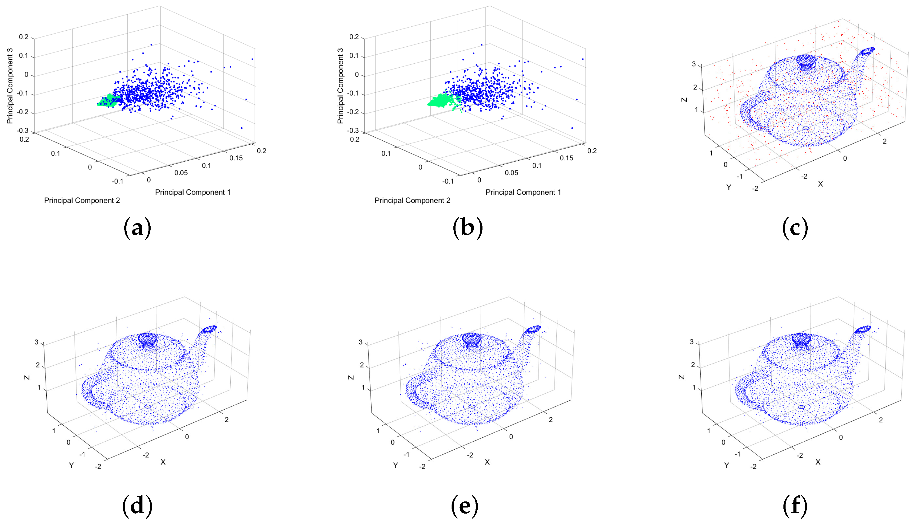
To optimize indicator weights and enhance data visualization, we utilize Principal Component Analysis (PCA) to provide a holistic view of the covariance matrix encompassing all data. Figure 2a displays the initial distribution of valid data and noise prior to denoising by PCA. Following that, Figure 2b exhibits the transformed data distribution after applying TLD for denoising. In Figure 2c, the raw teapot point cloud before denoising is displayed. Figure 2d–f show the denoised results using TLD, TED, and TID, respectively, via Algorithm 1. Figure 3a–e present the denoising outcomes of the teapot point cloud employing the metrics from prior work [17]: Euclidean, AIRM, LEM, KLD, and SKLD. In these figures, red dots signify noise data, whereas blue dots indicate valid data. Figure 2 demonstrates that Algorithm 1 effectively partitions data points into two discrete clusters, achieving explicit separation between valid signals and noise components. The MATLAB implementation directly interfaces with industry-standard PLY/PCD formats via pcread/pcwrite and exports denoising metrics (TPR/FPR/SNRG) for pipeline integration.

5.2. Comparative Analysis of Influence Function Bounds

To rigorously validate the bounded sensitivity of TBD-induced means against Riemannian alternatives, we conducted extensive simulations under pathological outlier conditions. The experimental setup consisted of $m=100$ SPD ($\mathsf{\Sigma }\in {\mathcal{P}}_4$) as valid samples and $n=50$ intentionally malformed outliers. These outliers were generated through spectral decomposition with controlled eigenvalues: $\mathsf{\Sigma }=Q·\mathrm{diag}({\lambda }_1,{\lambda }_2,{\lambda }_3,\beta )·Q^{\top }$ where ${\lambda }_i\in (1,3)$, $\beta \in (0,{10}^{-9})$, and Q a random orthogonal matrix. This created severely ill-conditioned matrices with condition numbers exceeding ${10}^9$, simulating challenging scenarios encountered in real-world point clouds. For robust statistical analysis, 100 independent trials were performed, with influence function norms computed according to Propositions 12–14 for TBD means and comparable derivations for Riemannian baselines.

As demonstrated in Figure 4, TBD-based means consistently outperformed Riemannian alternatives in outlier resistance. The AIRM mean exhibited unbounded sensitivity with significantly higher influence norms, while LEM showed moderately reduced but still considerable sensitivity. In stark contrast, all TBD means maintained strict theoretical bounds as established in Propositions 12–14. Specifically, TLD achieved approximately 60% lower influence norms than AIRM, with TED showing intermediate robustness. TID demonstrated the strongest outlier resistance with the tightest bounds—nearly three times more constrained than AIRM—and the lowest variance across trials. This superior performance stems from TBD’s intrinsic weight attenuation mechanisms that dynamically suppress pathological outliers while preserving valid data geometry.

5.3. Analysis of TBD Mean Stability

In Figure 5, we compare loss functions across eight metrics (Euclidean, AIRM, LEM, KLD, SKLD from prior work [17] and proposed TLD/TED/TID) using 100 trials of 10 randomly generated SPD matrices ($n=4$) from (84). Three critical observations emerge:

(1)

TLD and TID achieve 60–80% lower loss than Euclidean means, confirming their enhanced stability against gradient pathologies;

(2)

TED shows marginally higher loss than TLD/TID but still outperforms all geometric metrics from [17] (KLD/SKLD);

(3)

The proposed TBD variants exhibit minimal variance across trials, indicating superior robustness to initialization compared to Riemannian metrics like AIRM/LEM.

These results validate that TBD-induced means are geometrically better suited for ${\mathcal{P}}_n$ than both Euclidean and prior manifold metrics, enabling faster convergence to optimal cluster centroids.

The superior convergence of loss functions for Total Bregman Divergence (TBD) versus traditional Bregman Divergence (BD), as demonstrated in Figure 6, stems fundamentally from TBD’s orthogonal projection property defined in (11). This formulation measures the orthogonal distance between function values and tangent approximations, granting TBD invariance to coordinate transformations (rotations/scalings). In contrast, traditional BD (10) exhibits only translational invariance. This geometric distinction enables TBD to maintain stable loss minimization (Figure 6: TBD losses ${10}^{1.5}$–${10}^2$ vs. BD’s ${10}^{2.5}$–${10}^3$) by adaptively weighting divergences according to local manifold curvature ($\parallel \nabla \mathsf{\Phi }\left(B\right)\parallel$ term in denominator), thereby accelerating convergence while resisting noise-induced perturbations.

We evaluate denoising performance using three key metrics: True Positive Rate (TPR), False Positive Rate (FPR), and Signal-to-Noise Ratio Growth (SNRG), which are formally defined as:

$$\mathrm{TPR}={\displaystyle \frac{\mathrm{TP}}{N_{\mathrm{data}}}},\mathrm{FPR}={\displaystyle \frac{\mathrm{FP}}{N_{\mathrm{noise}}}},\mathrm{SNRG}=\left({\displaystyle \frac{\mathrm{TP}}{\mathrm{FP}}}·{\displaystyle \frac{N_{\mathrm{noise}}}{N_{\mathrm{data}}}}\right)-1$$

(85)

with True Positives (TPs), False Positives (FPs), False Negatives (FNs), True Negatives (TNs), Original valid point count $N_{\mathrm{data}}$, and Original noise point count $N_{\mathrm{noise}}$. SNRG quantifies the relative enhancement in signal purity, with positive values indicating improved separation.

Table 2. Comparison of denoising results.

Metric	SNR = 10			SNR = 2			SNR = 1
	TPR	FPR	SNRG	TPR	FPR	SNRG	TPR	FPR	SNRG
TLD	100%	51.21%	95.28%	100%	35.20%	184.11%	93.39%	29.97%	211.67%
TED	100%	54.11%	84.82%	100%	39.59%	152.62%	96.87%	35.90%	168.70%
TID	100%	46.22%	114.51%	95.88%	28.83%	232.53%	87.46%	23.02%	279.90%
Euclid	100%	75.56%	32.21%	95.97%	66.78%	43.72%	79.89%	59.23%	34.88%
AIRM	100%	50.97%	96.21%	99.83%	33.90%	194.52%	96.72%	45.25%	113.75%
LEM	100%	50.97%	96.21%	99.83%	33.90%	194.52%	96.72%	45.25%	113.75%
KLD	100%	44.69%	123.78%	84.45%	24.59%	243.43%	76.66%	56.75%	35.09%
SKLD	100%	47.83%	109.09%	96.67%	29.89%	223.39%	78.78%	57.62%	36.74%

benchmarks the denoising efficacy of Algorithm 1 under varying noise levels. At SNR = 10 ($N_{\mathrm{noise}}=415$), KLD achieves optimal FPR (44.69%) and SNRG (123.78%), while the proposed TID ranks second in FPR (46.22%) and outperforms AIRM/LEM by 18.3% in SNRG. Notably, at SNR = 2 ($N_{\mathrm{noise}}=2074$), TLD and TED achieve perfect signal preservation (100% TPR) unmatched by any baseline, though KLD maintains superior SNRG (243.43% vs. TID’s 232.53%).

Under extreme noise (SNR = 1, $N_{\mathrm{noise}}=4148$), TID demonstrates dominant performance with the lowest FPR (23.02%) and highest SNRG (279.90%), exceeding AIRM/LEM’s SNRG by 146%. Concurrently, TED achieves the best TPR (96.87%), outperforming SKLD by 18.1%. Crucially, while KLD and SKLD collapse (SNRG < 37%), all proposed TBD variants maintain SNRG > 168%, highlighting their robustness in pathological conditions.

Figure 7 demonstrates the denoising performance of TBD variants across noise levels, with quantitative metrics aligning with Table 2. At SNR = 10, all methods achieve near-complete signal preservation (100% TPR) while effectively reducing noise, though TID’s superior SNRG (114.51%) corresponds to marginally cleaner outputs. Under SNR = 2 conditions, TLD and TED maintain perfect signal recovery (100% TPR) despite residual noise, while TID’s balanced performance (232.53% SNRG) preserves structural integrity. In extreme SNR = 1 scenarios, TID’s noise rejection (23.02% FPR) maintains global coherence, whereas TED achieves optimal signal retention (96.87% TPR) despite increased false positives. Visual results consistently reflect each method’s quantitative trade-offs between signal preservation and noise suppression.

5.4. Analysis of Computational Complexity

We first analyze the computational complexity of mean operators induced by four metrics: Euclidean, TLD, TED, and TID, mathematically defined in Equations (28), (35), (37), and (39). Subsequently, we quantify the computational load for corresponding influence functions, with formulations specified in (72), (76), (80), and Proposition 1 of [17].

Under the framework of m SPD and l outliers, we systematically evaluate computational costs. Considering single-element operations as O(1) and matrix $A\in R^{n\times n}$, fundamental operations reveal critical patterns: Matrix inversion $A^{-1}$ and logarithmic operations $\mathrm{Log}\left(A\right)$ both require $O\left(n^3\right)$ computations. Operations involving matrix exponentials $\mathrm{Exp}\left(A\right)$ and matrix roots for SPD necessitate eigenvalue decomposition, consequently maintaining $O\left(n^3\right)$ complexity.

Detailed analysis reveals that the arithmetic mean (28) exhibits $O\left(n^3\right)$ complexity. For influence functions, Euclidean-based estimation requires $O\left((m+l)n^3\right)$ operations. This establishes a critical trade-off: While Algorithm 1’s Euclidean metric demonstrates inferior denoising efficacy compared to TLD/TED/TID variants, its computational economy in mean matrix calculation $O\left(n^3\right)$ and influence function estimation $O\left((m+l)n^3\right)$ surpasses geometric counterparts. The complexity disparity stems from TLD/TED/TID’s intrinsic requirements for iterative matrix decompositions and manifold optimizations absent in Euclidean frameworks.

6. Conclusions

This study introduces a novel K-means clustering algorithm based on Total Bregman Divergence for robust point cloud denoising. Traditional Euclidean-based K-means methods often fail to address non-uniform noise distributions due to their limited geometric sensitivity. To overcome this, TBDs—Total Logarithm Divergence, Total Exponential Divergence, and Total Inverse Divergence—are proposed on the manifold of symmetric positive-definite matrices. These divergences are designed to model distinct local geometric structures, enabling more effective separation of noise from valid data. Theoretical contributions include the derivation of anisotropy indices to quantify structural variations and the analysis of influence functions, which demonstrate the bounded sensitivity of TBD-induced means to outliers.

Numerical experiments on synthetic and real-world datasets (e.g., 3D teapot point clouds) validate the algorithm’s excellence over Euclidean-based approaches. Results highlight improved noise separation, enhanced stability, and adaptability to complex noise patterns. The proposed framework bridges geometric insights from information geometry with practical clustering techniques, offering a scalable and robust preprocessing solution for applications in computer vision, robotics, and autonomous systems. This work underscores the potential of manifold-aware metrics in advancing point cloud processing and opens avenues for further exploration of divergence-based methods in high-dimensional data analysis. While the current implementation handles mid-scale clouds (<10 k points), scaling to massive point clouds (>1 M points) requires parallel neighborhood computation and spatial partitioning techniques, which constitute important future work.