CLB-BER: An Approach to Electricity Consumption Behavior Analysis Using Time-Series Symmetry Learning and LLMs

Abstract

This study proposes an application framework based on Large Language Models (LLMs) to analyze multimodal heterogeneous data in the power sector and introduces the CLB-BER model for classifying user electricity consumption behavior. We first employ the Euclidean–Cosine Dynamic Windowing (ECDW) method to optimize the adjustment phase of the CLUBS clustering algorithm, improving the classification accuracy of electricity consumption patterns and establishing a mapping between unlabeled behavioral features and user types. To overcome the limitations of traditional clustering algorithms in recognizing emerging consumption patterns, we fine-tune a pre-trained DistilBERT model and integrate it with a Softmax layer to enhance classification performance. The experimental results on real-world power grid data demonstrate that the CLB-BER model significantly outperforms conventional algorithms in terms of classification efficiency and accuracy, achieving 94.21% accuracy and an F1 score of 94.34%, compared to 92.13% accuracy for Transformer and lower accuracy for baselines like KNN (81.45%) and SVM (86.73%); additionally, the Improved-C clustering achieves a silhouette index of 0.63, surpassing CLUBS (0.62) and K-means (0.55), underscoring its potential for power grid analysis and user behavior understanding. Our framework inherently preserves temporal symmetry in consumption patterns through dynamic sequence alignment, enhancing its robustness for real-world applications.

1. Introduction

A power system, being a critical infrastructure, requires precise and efficient analysis tools to ensure its stable and reliable operation. The accurate analysis of electricity consumption patterns, timely fault diagnosis, and efficient resource allocation are essential for the optimal performance of power systems. Traditional power system analysis methods face significant bottlenecks, such as reliance on static models, limited data processing capacity, subjective human intervention, and inefficiency in adapting to complex changes. The intricacy and magnitude of contemporary power systems, along with the incorporation of renewable energy sources and the increasing penetration of distributed generation, pose significant challenges to traditional analytical methods.

In the power sector, data is often characterized by its multi-source, heterogeneous, and massive nature. This includes data from smart meters, grid sensors, weather stations, and market transactions, among others. Such data is not only voluminous but also highly variable in terms of format and quality, making it difficult for traditional methods to process and analyze effectively. Traditional methods struggle to handle the diverse and complex nature of this data, often resulting in inefficient and inaccurate analysis. These challenges necessitate the adoption of more advanced techniques capable of managing and unlocking valuable insights from these elaborate datasets.

In the past decade, the application of machine learning and AI techniques to research on problems in the power field has achieved promising results. For instance, Wang et al. [1] proposed a data-driven DDRO distribution scheduling method based on the spatial correlation between multiple wind farm outputs to achieve optimal scheduling. Li et al. [2] introduced a VAE-SSA-PNN fault diagnosis model for distribution Transformers, employing a variable autoencoder (VAE), methods for non-coding reduction, and PCA to sequentially refine fault data within the PNN framework, enabling the efficient and fast diagnosis and prediction of Transformer status. Huang et al. [3] proposed a robust graph convolutional neural network to address the vulnerability of AI models used in power image classification and recognition to adversarial perturbations. Liu et al. [4] developed a blockchain scheme based on differential privacy for secure power data transactions, achieving privacy protection, transaction security, and data reliability.

Despite the promising potential of these methods, they encounter several limitations. These methods often require extensive domain-specific feature engineering, which is time-consuming and might lack robustness when applied to diverse datasets. They struggle with integrating and processing the diverse, heterogeneous, and massive data inherent in modern power systems. Traditional AI models lack the flexibility to adapt to new patterns or anomalies in electricity consumption without substantial retraining, leading to inefficiencies in dynamic and real-time applications. Moreover, existing studies often address isolated problems, making it difficult to form a unified application paradigm for the power field. Consequently, current research has not achieved satisfactory results in handling massive multi-source heterogeneous data comprehensively.

Currently, LLMs like BERT and GPT are catalyzing significant advancements in natural language processing (NLP). These models are complex deep learning constructs built upon the Transformer architecture [5]. With their parameters extending into the tens of billions, LLMs are celebrated as they have led to monumental strides in AI in recent times [6]. Notably, the GPT series developed by OpenAI exemplifies these innovations. The core advantage of LLMs is their proficiency in deciphering latent information from prompts and crafting pertinent responses. This ability is rooted in their extensive pre-training on diverse corpora and the foundational Transformer architecture. LLMs exhibit robust performance across a spectrum of NLP tasks by adapting to linguistic cues [7,8]. Furthermore, LLMs can adeptly handle novel tasks with minimal adaptation, leveraging the Few-shot learning paradigm, thereby demonstrating their versatility and efficacy without the necessity for additional training. In the field of electricity, the prospective applications of LLMs are extensive. Their powerful representation capabilities and flexible transfer learning methods can be effectively applied to electricity consumption pattern analysis, power equipment fault diagnosis, and user feedback analysis. By integrating LLMs with other data processing and analysis technologies, the intelligence level and operational efficiency of power systems can be significantly enhanced. Specifically, LLMs can address the limitations of traditional AI models by providing more generalized and adaptive solutions, reducing the need for extensive feature engineering, and efficiently handling heterogeneous and massive datasets.

While prior works have explored LLMs for time-series data, such as reprogramming LLMs for forecasting tasks [9] or leveraging pre-trained LLMs to capture complex dependencies in time series for applications like anomaly detection [10], these approaches often focus on predictive modeling rather than behavioral classification. For instance, studies in power systems have applied LLMs to load forecasting [11] and advanced dispatch optimization [12], but they typically overlook the integration of clustering for unlabeled pattern mapping with fine-tuned LLMs for downstream classification. Moreover, recent evaluations question the inherent utility of LLMs in preserving temporal structures for time-series tasks without domain-specific enhancements [13]. In contrast, our CLB-BER model introduces novelty by combining an ECDW-optimized CLUBS clustering algorithm—which dynamically aligns sequences while preserving temporal symmetry—with a fine-tuned DistilBERT for the robust classification of emerging electricity consumption patterns. This pipeline not only bridges unsupervised clustering with supervised LLM-based classification, but also outperforms traditional pipelines in handling multimodal heterogeneous power data, as demonstrated in our experiments.

This paper explores the application of LLMs in classifying the electricity consumption patterns of users. We propose a novel method that integrates the improved CLUBS clustering algorithm with a fine-tuned BERT model, enhanced with a Softmax layer for downstream classification tasks, to improve the accuracy and efficiency of electricity consumption pattern classification. Comparative experiments demonstrate the effectiveness of this method in handling complex data and identifying new user consumption patterns.

The primary contributions of this paper are as follows:

• We propose a novel LLM-based framework for the power sector with domain-specific fine-tuning to enhance distributed energy resource management, addressing the challenges of increasingly decentralized and complex energy systems.
• We enhance the CLUBS clustering algorithm with the innovative ECDW method while maintaining Spark compatibility, enabling the more accurate classification of diverse electricity consumption patterns.
• We develop CLB-BER, an advanced LLM-based classification model that employs our Improved-C algorithm, to label datasets and fine-tune a pre-trained DistilBERT model. By incorporating a Softmax layer, it achieves superior user classification accuracy in downstream tasks compared to conventional methods.

The organization of this paper is as follows: Section 2 presents the application framework based on LLMs. Section 3 elaborates on the improved CLUBS clustering algorithm and the integration of DistilBERT. Section 4 provides an experimental evaluation of the proposed model using extensive user electricity consumption data from a local power grid. Finally, Section 5 summarizes the findings and outlines directions for future research.

2. Methods and Framework

2.1. Overview of LLMs

Transformer-based Large Language Models (LLMs) are intricate systems equipped with extensive parameter sets, often exceeding hundreds of billions. These models are refined through the extensive analysis of vast textual datasets, leading the charge in natural language processing (NLP) advancements [14]. LLMs are applied across various sectors, including risk assessment [15], programming [16], vulnerability detection [17], medical text analysis [18], and search engine optimization [19]. Proprietary models like OpenAI’s GPT-4 [20] and Anthropic’s Claude [21] are accessible via web services or APIs, yet their parameters remain undisclosed. Conversely, open-source alternatives, like Meta AI’s Codellama series [22] and Stanford’s Alpaca [23], are fully disclosed and downloadable for local deployment. Organizations may offer infrastructures to support local usage, such as Codellama, with many also hosted on the Huggingface Hub, a collaborative repository featuring over 120 k LLMs [24].

BERT is an important representative of LLMs. The architecture of BERT centers on a multi-layer Transformer encoder, employing self-attention to analyze complex relationships across tokens and sentences, enhancing its linguistic comprehension capabilities. Illustrated in Figure 1, BERT processes inputs that include token, position, and sentence IDs. These inputs are transformed by the embedding layer into corresponding embeddings, which are then aggregated to form a comprehensive input representation. During its pre-training phase, BERT utilizes a masked language model (MLM) strategy, obscuring select tokens at random to facilitate the prediction of their original forms.

The training process of LLMs typically includes several stages: data collection and preprocessing, model pre-training, fine-tuning, and evaluation. Initially, the model is pre-trained on large-scale datasets to acquire extensive language knowledge. Subsequently, it undergoes fine-tuning for specific tasks to optimize performance. Finally, the model is validated using various evaluation metrics to ensure its effectiveness.

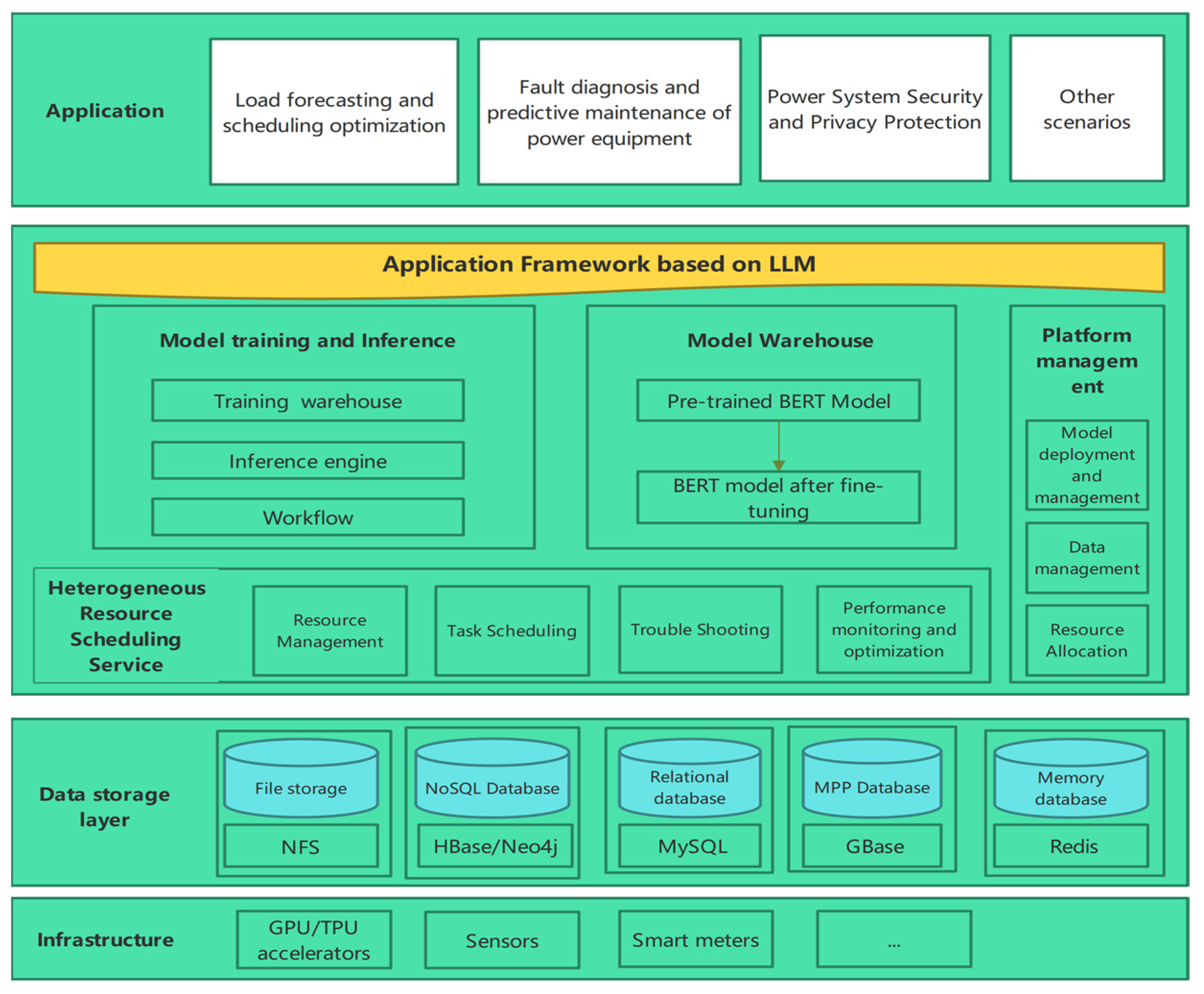
2.2. Application Framework Based on LLMs

The Application Framework based on LLMs is structured into six layers, as illustrated in Figure 2: the hardware layer, data storage layer, heterogeneous resource scheduling service layer, model training and inference layer, model repository layer, and platform management layer.

The specific content of the platform is as follows:

(1)

The hardware layer integrates GPUs, TPUs, sensors, and smart meters for efficient computational power and data collection from the power system and customers. This layer additionally comprises a data collection interface and a data transmission module.

(2)

The data storage layer utilizes the NFS, HBase/Neo4j, MySQL, GBase, and Redis databases to stores massive multi-source heterogeneous data. NFS offers distributed file systems for large-scale data storage and retrieval. HBase and Neo4j store structured and unstructured data, respectively. MySQL and GBase manage structured business data, while Redis stores temporary and cache data.

(3)

The heterogeneous resource scheduling service layer manages resource allocation, task scheduling, troubleshooting, and performance monitoring and optimization. It oversees computing assets like CPUs, GPUs, and TPUs, arranges computational tasks, detects and resolves system issues, and optimizes system performance.

(4)

The model training and inference layer includes a training warehouse, an inference engine, and a workflow for managing training datasets, deploying trained models for real-time or batch inference, and defining and overseeing model training and inference progress with complex workflows.

(5)

The model warehouse stores pre-trained LLMs, such as BERT, along with fine-tuned models tailored to specific application scenarios.

(6)

The platform management layer includes model deployment and management, data management, and resource allocation.

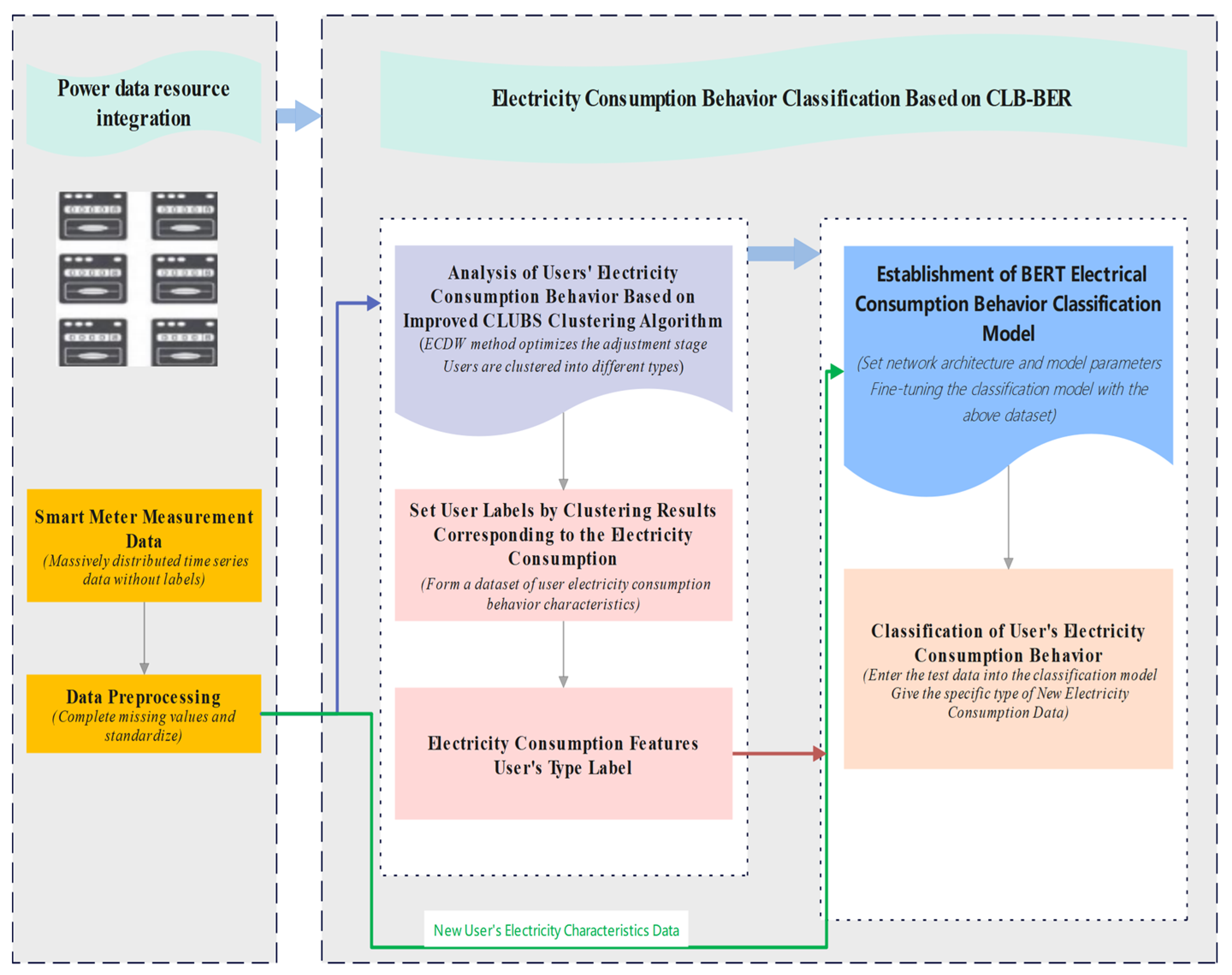
3. Electricity Consumption Behavior Classification Based on CLB-BER

The electricity usage behavior classification model framework is illustrated in Figure 3. The framework comprises three primary steps: (1) data collection and preprocessing; (2) the classification of electricity consumption behavior; (3) construction and tuning of the BERT model.

Firstly, relying on smart meters, a substantial volume of customer electricity usage time-series data is collected and processed to address missing values and outliers. Specifically, for the missing values present in the data, various methods are employed to impute them, such as linear interpolation, moving average, or other filling methods applicable to time-series data, ensuring data continuity. Outliers in the data, often resulting from sensor failures or data transmission errors, are detected and handled using statistical methods or machine learning algorithms to ensure accurate data correction. Secondly, the improved CLUBS clustering algorithm is applied to classify the electricity consumption behavior. Finally, the pre-trained BERT is introduced and fine-tuned by clustering labels. Then, the intelligent classification model is successfully developed.

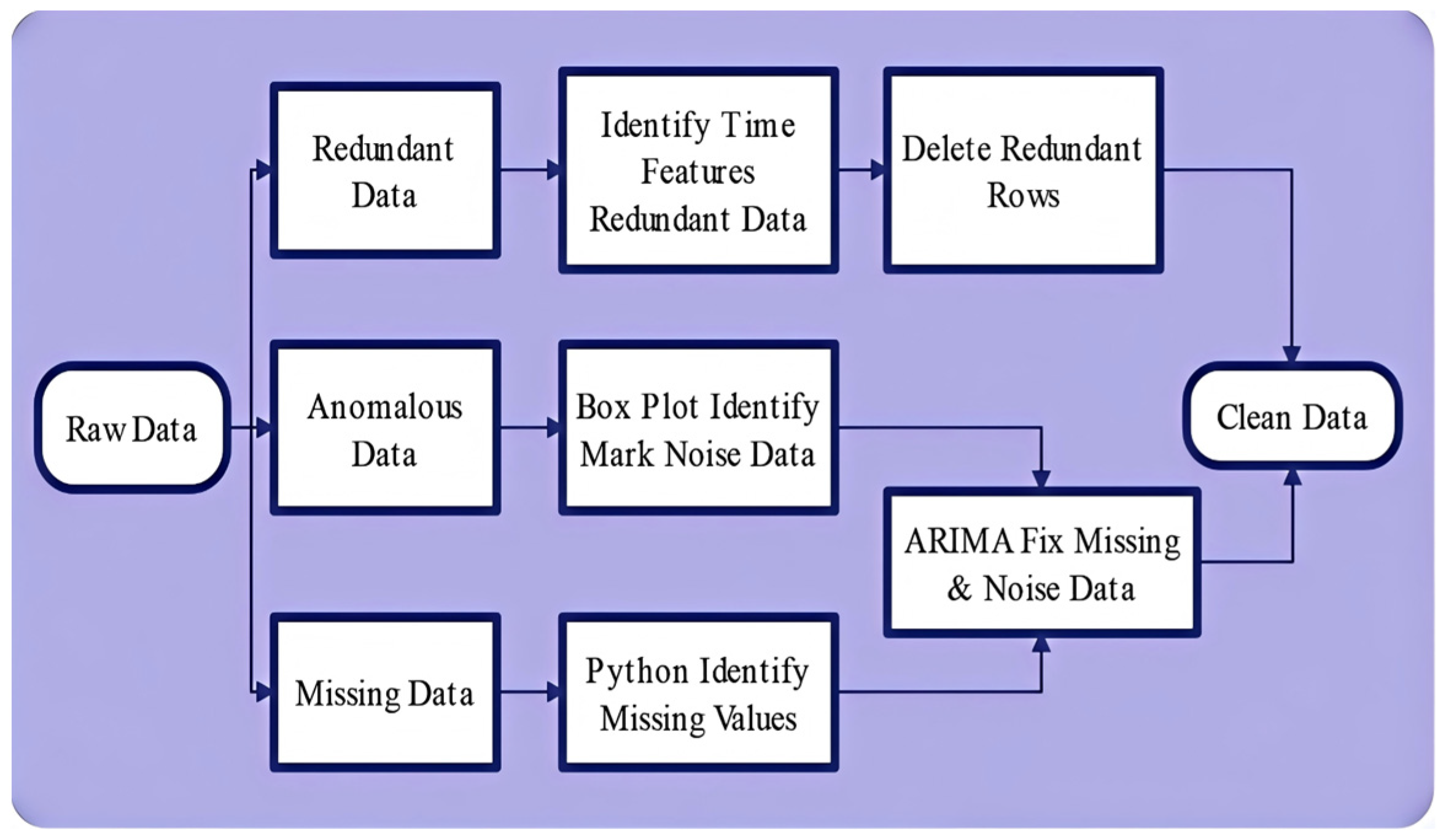
3.1. Data Preprocessing

The data processing steps are shown in Figure 4. In view of data redundancy, anomalous and missing cases in the original data, the processing methods will be elaborated upon in the following section.

3.1.1. Noise Recognition

Noise is the abnormal data in the dataset. The existence of abnormal data makes training more difficult, makes the trained model deviate, and makes the direction of deviation uncertain, resulting in inaccurate results. In this paper, box plots are used to identify and mark the noise points. The mathematical expression formula of the box plots is shown in Equations (1)–(4).

$$Q1=\left\{\begin{array}{ll}\mathit{Median} \mathit{of} X_1,X_2,\dots ,X_{\left(n-1\right)/2}\hfill & \mathit{if} n \mathit{is} \mathit{odd}\hfill \\ \mathit{Median} \mathit{of} X_1,X_2,\dots ,X_{n/2}\hfill & \mathit{if} n \mathit{is} \mathit{even}\hfill \end{array}\right.$$

(1)

$$Q3=\left\{\begin{array}{ll}\mathit{Median} \mathit{of} X_{\left(n+3\right)/2},X_{\left(n+5\right)/2},\dots ,X_n\hfill & \mathit{if} n \mathit{is} \mathit{odd}\hfill \\ \mathit{Median} \mathit{of} X_{\left(n/2\right)+1},X_{\left(n/2\right)+2},\dots ,X_n\hfill & \mathit{if} n \mathit{is} \mathit{even}\hfill \end{array}\right.$$

(2)

$$\left\{\begin{array}{l}\mathit{IQ}=Q_3-Q_1\hfill \\ \mathit{Vmin}=Q_1-1.5 IQR\hfill \\ \mathit{Vmax}=Q_3+1.5 IQR\hfill \end{array}\right.$$

(3)

$$V=\left\{\begin{array}{l}\mathit{Normal} \mathit{values}, \mathit{Vmin}<V<Vmax\hfill \\ Outliers, V>Vmax, V<Vmin\hfill \end{array}\right.$$

(4)

where $V_{min}$ is the lower end of the numerical range, $V_{max}$ denotes the upper end of the numerical range, $Q_1$ represents the lower quartile, $Q_3$ is the upper quartile, and IQR is the interquartile range.

3.1.2. Missing and Noise Value Repair

ARIMA is a widely used statistical model for time-series analysis and forecasting. The ARIMA model combines three components: autoregression (AR), differencing (I), and moving average (MA). It is suitable for modeling and predicting data that exhibits non-stationarity, which means its statistical properties change over time.

$$X_t={\varphi }_1{X}_{t-1}+{\varphi }_2{X}_{t-2}+\cdots +{\varphi }_p{X}_{t-p}+{ϵ}_t$$

(5)

where ${\varphi }_1,{\varphi }_2,\dots ,{\varphi }_p$ are the parameters, and ${ϵ}_{\mathrm{t}}$ is white noise.

Integrated (l) Part: This part involves differencing the raw observations to make the time series stationary.

$$Y_t={\mathsf{\nabla }}^d{X}_t={\left(1-B\right)}^d{X}_t$$

(6)

where ${\mathsf{\nabla }}^d$ denotes differencing $d$ times, and $B$ is the backshift operator, defined as $B{X}_t=X_{t-1}.$

$${ϵ}_t={\theta }_0+{\theta }_1{ϵ}_{t-1}+{\theta }_2{ϵ}_{t-2}+\cdots +{\theta }_q{ϵ}_{t-q}$$

(7)

where ${\theta }_0,{\theta }_1,\dots ,{\theta }_q$ are parameters.

The full ARIMA model combines these three parts, as shown in (8).

$${\Delta }^d{y}_t={\varphi }_1{\Delta }^d{y}_{t-1}+{\varphi }_2{\Delta }^d{y}_{t-2}+\cdots +{\varphi }_p{\Delta }^d{y}_{t-p}+{ϵ}_t+{\theta }_1{ϵ}_{t-1}+{\theta }_2{ϵ}_{t-2}+\cdots +{\theta }_q{ϵ}_{t-q}$$

(8)

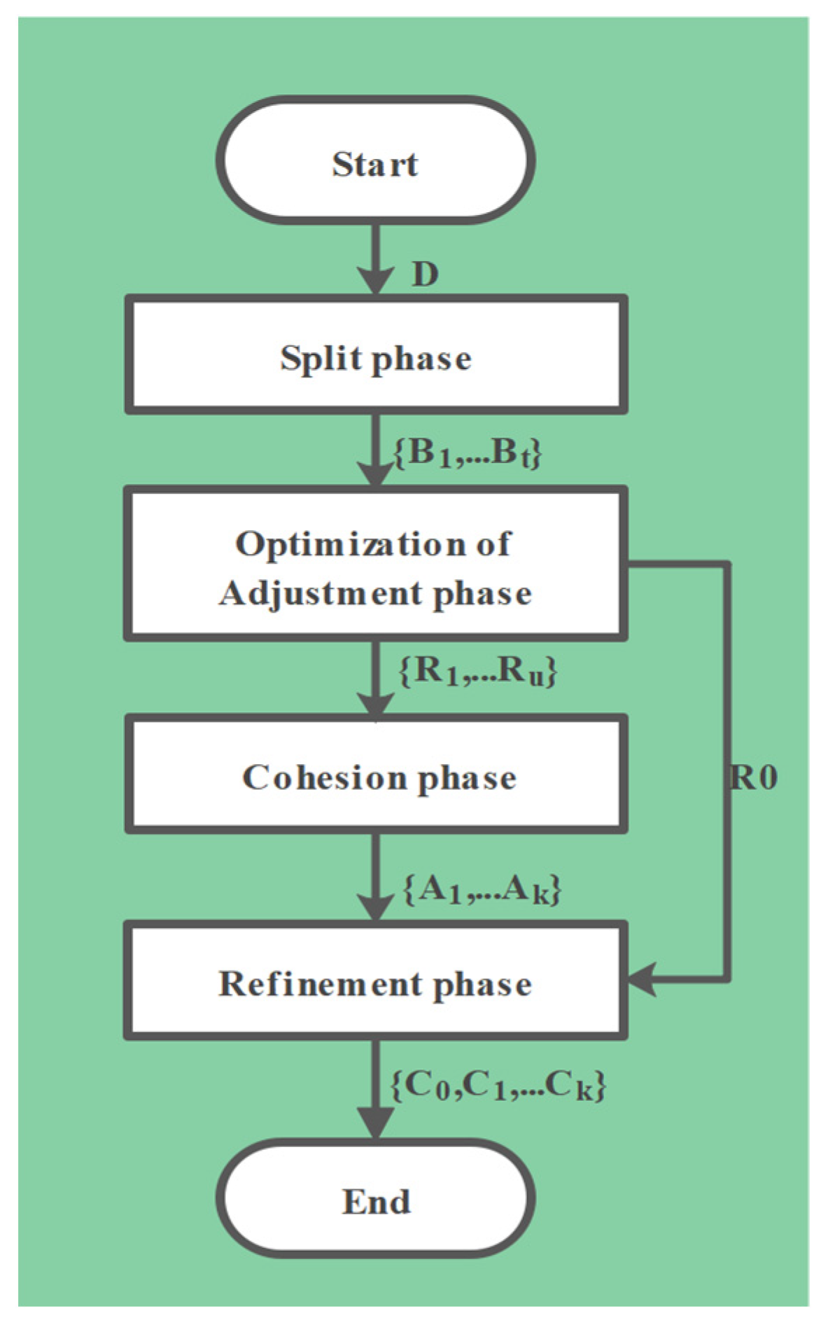
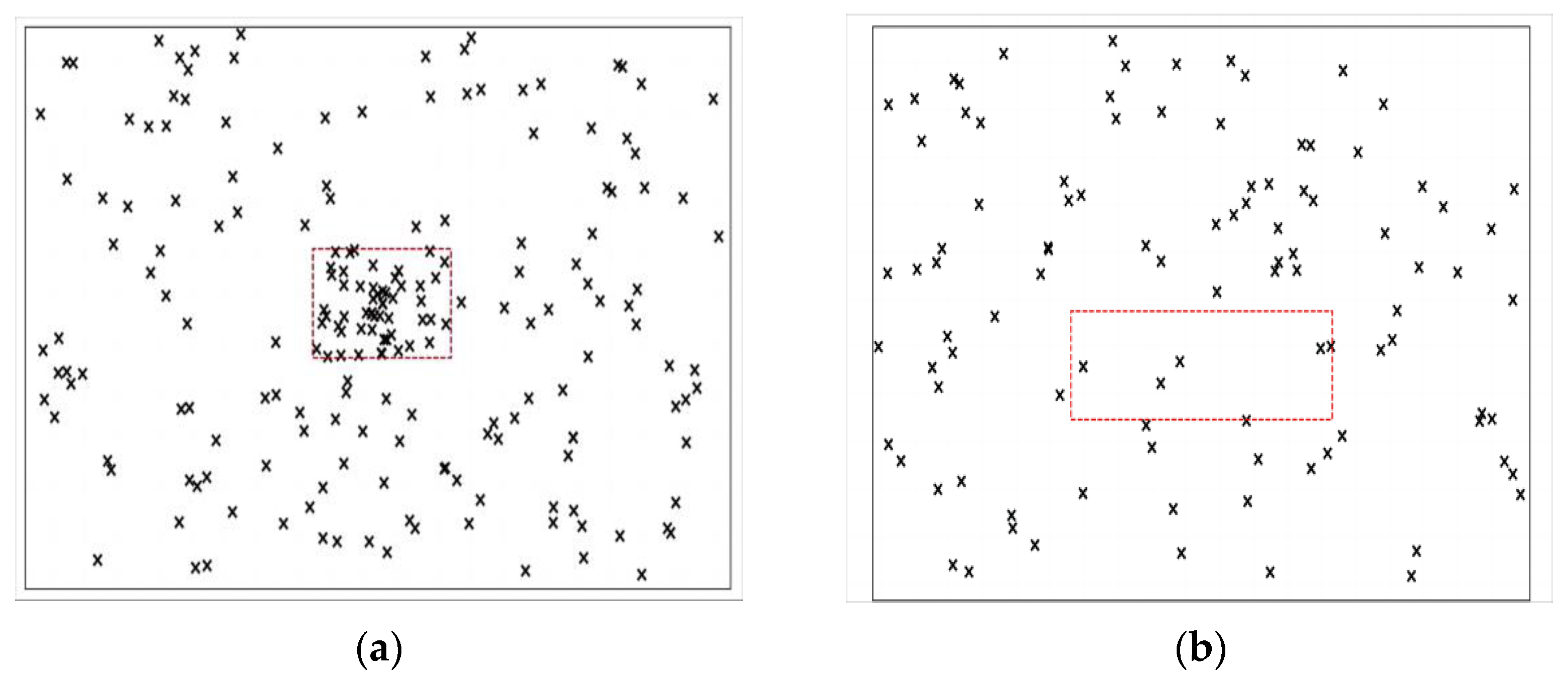
3.2. Improved CLUBS Clustering

The Improved-C algorithm is an improved version of CLUBS, as illustrated in Figure 5. We replace the traditional Euclidean distance with the ECDW method to solve the problem of sequence length mismatch and sequence shape differences that are too large, caused by pure clustering calculation, and optimize the clustering quality in the adjustment stage. The Improved-C algorithm [25] is a non-parametric clustering method employing a rapid hierarchical strategy to cluster data points around their centroid. The algorithm involves four main steps: (1) the split phase, (2) the optimization-of-adjustment phase, (3) the cohesion phase, and (4) the refinement phase.

3.2.1. Split Phase

Initially, the algorithm begins with the entire dataset within a single cluster S, which is subsequently inserted into a priority queue Q for iterative segmentation. As long as Q is not empty, the algorithm extracts a block B, dividing it into two sub-blocks. Should this division prove valid, these sub-blocks supplant B in Q; if not, B stands as the definitive block for that iteration. To optimize the segmentation, it is essential to evaluate the marginal distribution for each dimension i within block B, so it is necessary to compute the functions $C_B^i: ℝ\to N$ and $L{S}_B^l:ℝ\stackrel{I}{\to }{ℝ}^d$, as shown in Equations (9) and (10).

$$C_B^i\left(x\right)=\left|p\in B\wedge p\left[i\right]=x\right|$$

(9)

$$L{S}_B^i\left(x\right)={{\displaystyle \sum }}_{p\in B\wedge p\left[i\right]=x}p$$

(10)

We aggregate all the points p within block B, where the coordinates of the i-th dimension equal x. This aggregation can be depicted as either a graph or an array.

Minimizing the segmentation of WCSS can be achieved by performing a linear scan of the graph or array. The Kalinsky–Harabas (CH) index is used to assess the quality of clustering. After each segmentation, the CH value is recalculated. If the CH value increases, the splitting phase is deemed valid and proceeds; if the CH value decreases below 70%, the splitting is stopped.

$$WCSS\left(C\right)={{\displaystyle \sum }}_{i=1}^d\left(Q_i-{\displaystyle \frac{S_i^2}{n}}\right)$$

(11)

where $S_i={\displaystyle \sum }_{p\in C}{p}_i$ and $Q_i={{\displaystyle \sum }}_{p\in C}{p}_i^2$, respectively, denote the sum of the i-th coordinates and the sum of the squares of i-th coordinates of the points in C.

$\mathrm{Let} \mathrm{C} = \{C_1,\dots ,C_k\}$ be a set of clusters over a dataset $D=\left\{p_1,\dots ,p_n\right\}$, where the i-th $\left(1\le i\le k\right)$ cluster has $n_i$ points and centroid $\overline{c_i}$, and let $\overline{m}$ denote the centroid for the whole dataset $D.$ The BCSS (Between-Clusters Sum of Squares) of C is defined as

$$BCSS\left(C\right)={{\displaystyle \sum }}_{i=1}^k{n}_i\times {\parallel \overline{c_i}-\overline{m}\parallel }^2$$

(12)

$$CH-index\left(C\right)={\displaystyle \frac{BCSS\left(C\right)}{WCSS\left(C\right)}}\times {\displaystyle \frac{n-k}{k-1}}$$

(13)

$$\Delta WCSS\left(C^{ij}\right)={\displaystyle \frac{n_i·n_j}{n_i+n_j}}{{\displaystyle \sum }}_{k=1}^d{\left({\displaystyle \frac{S_{i,k}}{n_i}}-{\displaystyle \frac{S_{j,k}}{n_j}}\right)}^2$$

(14)

where $S_{i,k}\left(S_{j,k}\right)$ is the sum of the k-th coordinate (i.e., dimension) of all the points belonging to the cluster $C_i\left(C_j\right).$ This equation can be used to determine the increase in WCSS when a pair of clusters is merged into a single one.

3.2.2. Optimization-of-Adjustment Phase

Based on the conclusion of the splitting phase, the data space is segmented into two distinct types of blocks: one containing only a cluster and another containing only noise, as shown in Figure 6. In the adjustment phase, the CLUBS algorithm undertakes two tasks: (i) separating blocks containing clusters and (ii) forming an elliptic cluster from the separated blocks. Since noise-only blocks exhibit lower density, the first task can be achieved through density observation. CLUBS incrementally sorts all blocks by density and detects density jumps between neighboring blocks to identify potential subsets of noisy blocks. The candidate subset is then tested by creating a smaller hypercube at the centroid of the block. If the density within this hypercube significantly exceeds that of the entire block, the block is classified as noise-only. Otherwise, it is categorized as a cluster block.

Once all the cluster blocks have been identified, the process of forming comprehensive clusters for the remaining blocks and materializing the centroid of their clusters begins, and each data point is assigned to the cluster with the closest centroid. To achieve this, the approach in this paper employs a weighted function that considers the distance between points along each dimension. More specifically, this paper uses the centroid $\left(c_1,c_2,\mathrm{\dots },c_d\right)$ to measure the distance from each point $\mathrm{P}=\left(p_1,p_2,\mathrm{\dots },p_d\right)$ to each cluster block C.

$$dis{t}^{\star }\left(p,C\right)={{\displaystyle \sum }}_{i=1}^d{\left({\displaystyle \frac{\parallel p_i-c_i\parallel }{r_i}}\right)}^2$$

(15)

$$r_i=3\sqrt{{\displaystyle \frac{WCS{S}_i\left(C\right)}{n}}}$$

(16)

where n represents the count of points within cluster C, and $WCS{S}_i\left(c\right)$ denotes the variance in dimension i. Let $dis{t}^{\star }\left(p,C\right)=1$. Define an ellipse whose center is then the centroid of the cluster, and the radius of dimension i is then the radius of $r_i$.

The Euclidean distance solely measures point-to-point distances, neglecting the similarity in temporal patterns. Conversely, dynamic time warping (DTW) accounts for shape similarity, but overlooks temporal characteristics. The corresponding formula is as follows:

$$\begin{array}{ll}\mathrm{Dist}\left(\mathrm{Euclidean}\right)\hfill & =\sqrt{{\left({\mathrm{q}}_1-{\mathrm{c}}_1\right)}^2+{\left({\mathrm{q}}_2-{\mathrm{c}}_2\right)}^2+\cdots +{\left({\mathrm{q}}_{\mathrm{n}}-{\mathrm{c}}_{\mathrm{n}}\right)}^2}\hfill \\ \hfill & =\sqrt{{{\displaystyle \sum }}_{\mathrm{i}=1}^{\mathrm{n}}{\left({\mathrm{q}}_{\mathrm{i}}-{\mathrm{c}}_{\mathrm{i}}\right)}^2}\hfill \end{array}$$

(17)

$$\mathrm{Dist}\left(\mathrm{DTW}\right)=\min \left\{\sqrt{{{\displaystyle \sum }}_{\mathrm{k}=1}^{\mathrm{K}}{\mathrm{w}}_{\mathrm{k}}}/\mathrm{K}\right\}$$

(18)

In order to calculate the minimum distance between two time series, in this paper, we move the time-series data via a sliding window; the sliding window size equals the shorter time-series length, and the sliding step is 1. Cosine similarity is employed for initial similarity judgment, discarding data points that exceed the cosine similarity threshold. The Euclidean distance metric is then used to compute the distance among the windowed data. Ultimately, the function returns the smallest distance among the time series. This approach addresses the challenge of aligning points due to varying sequence lengths while considering both shape and distance similarity. This dynamic windowing intrinsically maintains symmetry constraints during shape alignment, optimizing pattern consistency without manual intervention. The pseudo code is as follows.

The Algorithm for Similarity Computation

1.   Procedure: Similarity computation(longTimeSeries, shortTimeSeries, cosineThreshold)   Input: longTimeSeries: the longer time series data         shortTimeSeries: the shorter time series data;         cosineThreshold: the threshold for cosine similarity;   Output: minDistance: the minimum distance between the two time series 2.   begin 3.     longLength ← length(longTimeSeries); 4.     shortLength ← length(shortTimeSeries); 5.     windowSize ← shortLength; 6.     minDistance ← +∞; 7.     //Step 1: Filter using cosine similarity 8.     for i from 0 to (long Length–short Length) do 9.        subSequence ← longTimeSeries[i: i + shortLength − 1]; 10.      cosineSim ← cosineSimilarity(subSequence, shortTimeSeries); 11.       if cosineSim ≥ cosineThreshold then 12.         //Step 2: Compute Euclidean distance using sliding window 13.         for j from 0 to (long Length–window Size) do 14.            subLongSequence ← longTimeSeries [j: j + windowSize − 1]; 15.            distance ← euclideanDistance(subLongSequence, shortTimeSeries); 16.            if distance < minDistance then 17.                minDistance ← distance; 18.            end 19.         end 20.      end 21.     end 22.     return minDistance; 23. end

3.2.3. Cohesion Phase

In the coalescence phase, clustering quality is enhanced through the amalgamation of clusters formed in the prior phase. If merging a pair of clusters results in a slight increase in WCSS and a significant increase in CH metrics, the cluster merge is considered valid. However, if the merger leads to a significant decrease in CH metrics, the merger is canceled and the coalescence phase ends. It is important to emphasize that solely mergers between adjacent clusters are taken into account, since only mergers of neighboring clusters may result in a slight increase in WCSS and a significant increase in CH metrics.

3.2.4. Refinement Phase

The coalescence phase guides the coalescence process only through the WCSS and CH metrics, which can result in slightly irregularly shaped clusters. During the refinement phase, the quality of clusters is enhanced, and outliers are removed by adapting the adjustment phase task 2 algorithm. The new CH calculation formula is given in Equation (19).

$$newCh={\displaystyle \frac{bcss-\Delta }{wcss+\Delta }}\times {\displaystyle \frac{n-k+1}{k-2}}$$

(19)

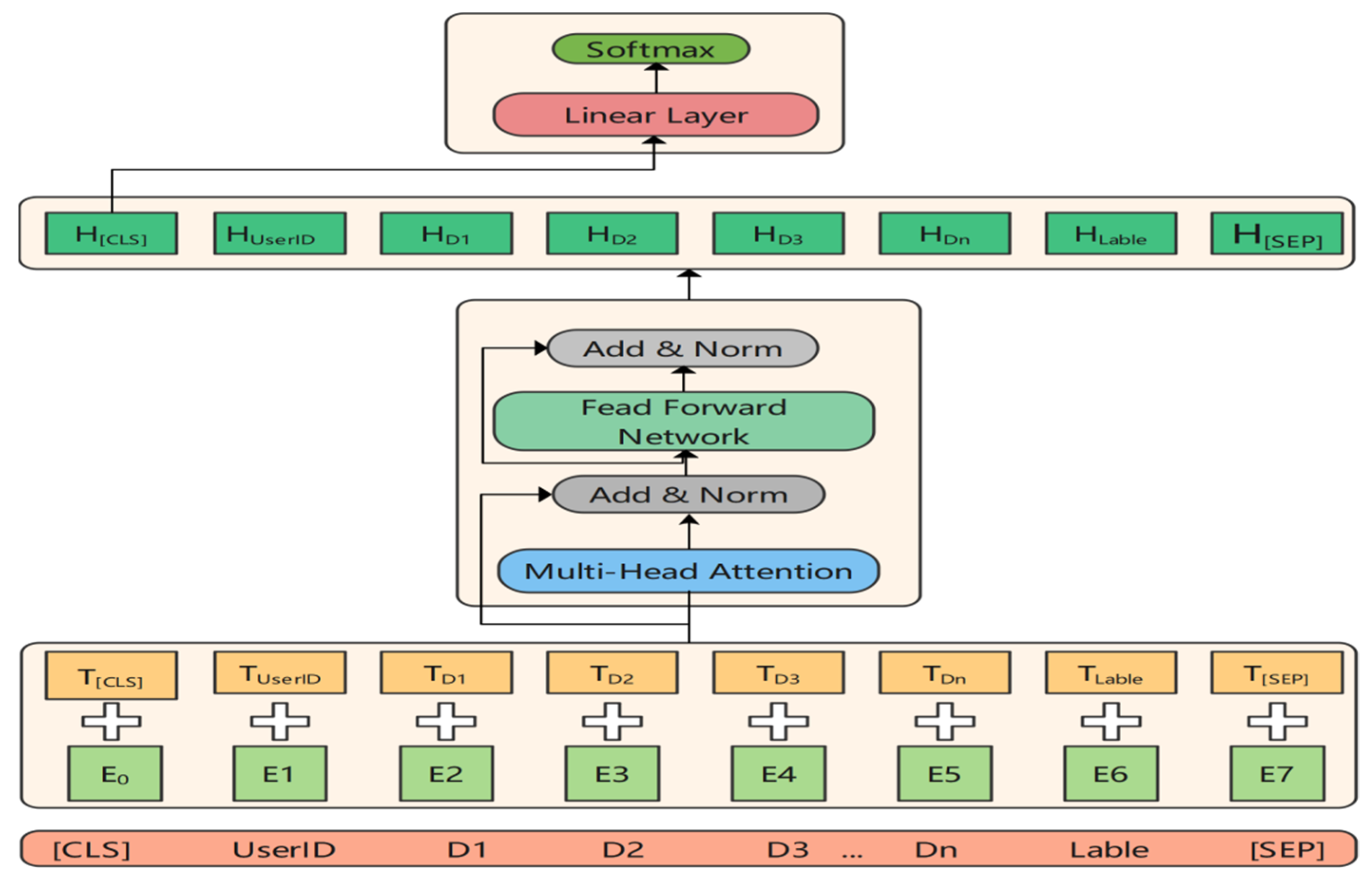
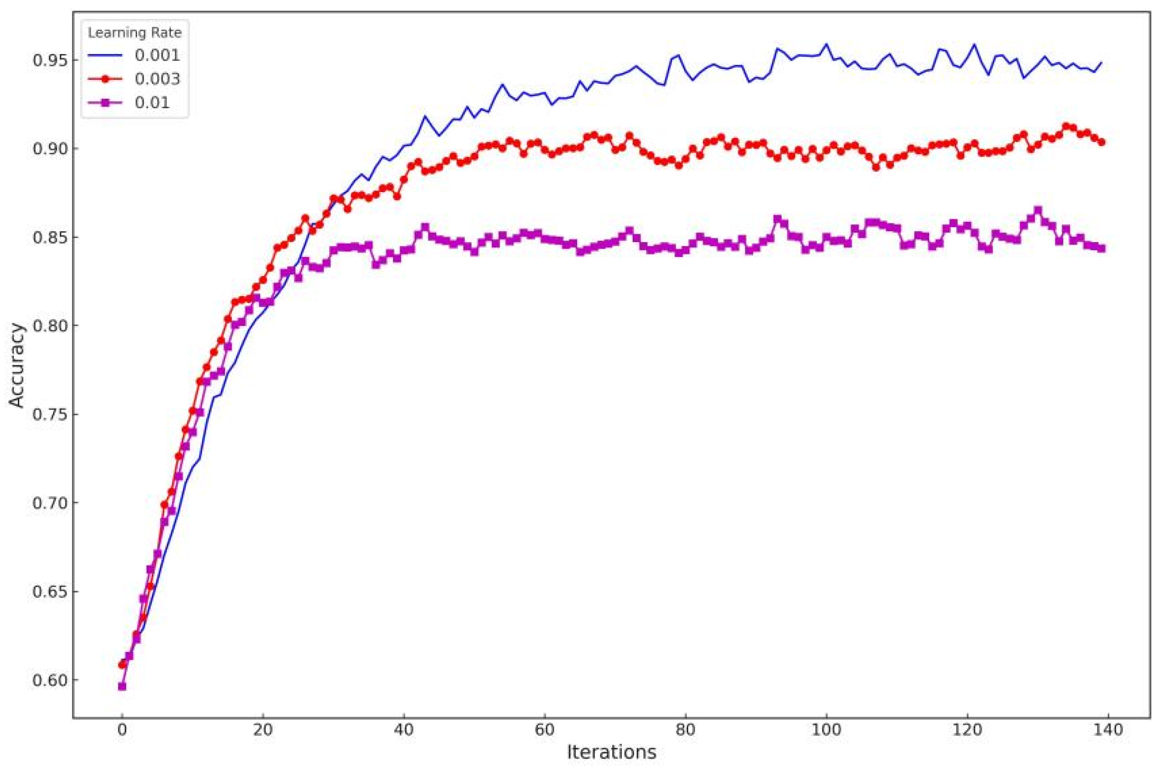
3.3. BERT Classification Model

Pre-trained BERT architectures, renowned for their efficacy, are amenable to both tuning and fine-tuning for diverse linguistic tasks, such as question answering and language identification [26]. BERT is acknowledged as a benchmark model in natural language processing due to its superior performance metrics across various tasks [27]. The adaptation process involves two critical phases: pre-training and fine-tuning. In the pre-training phase, BERT models are trained on a broad array of tasks using unlabeled data, facilitating the extraction of robust features. Subsequently, in the fine-tuning phase, these models are further optimized by adjusting pre-trained parameters using specifically prepared labeled data. Notably, the core architecture remains consistent across both phases, with modifications confined to the output layer to accommodate specific task requirements [28].

In this paper, we adopted the open-source pre-trained DistilBERT model for user electricity consumption behavior classification. DistilBERT is a stripped-down version of BERT with fewer parameters and faster training, but retains most of the performance of BERT. To enhance its classification performance, we embed the electricity consumption data, user ID, and month data into the model.

The architecture of DistilBERT is structured into three primary layers: the word embedding layer, the encoding layer, and the classification layer. The first layer integrates token, segmentation, and position embeddings to convert input data into vector representations. Subsequently, the encoding layer, comprising six Transformer units, transforms these embeddings into contextual representations, enhancing the model’s grasp of contextual semantics. Finally, the classification layer, which includes a fully connected layer and a Softmax layer, utilizes these contextual representations to classify and predict the appropriate categories. Figure 7 illustrates the DistilBERT classification model.

To adapt the numerical electricity consumption data for use with the DistilBERT model, we designed a tailored tokenization and embedding strategy. Since DistilBERT was originally designed for processing text inputs, we first transformed the monthly electricity usage values, user IDs, and month identifiers into a structured pseudo-sentence format using fixed templates. These structured sentences were then tokenized using the standard DistilBERT tokenizer, which mapped the text to token IDs based on pre-trained vocabulary.

After tokenization, the embedded vectors were generated via the DistilBERT embedding layer, which combined token, segment, and positional embeddings. This design ensures that the numerical information is contextually encoded, enabling the model to learn temporal and consumption-related patterns across different user behaviors.

Each input word $w_i$ is mapped to a high-dimensional vector space, resulting in the corresponding word embedding vector ${\mathrm{E}}_{\mathrm{token}}$ = TokenEmb(${\mathrm{w}}_{\mathrm{i}}$). To distinguish between the two sentences, BERT uses Segment Embedding to mark which sentence each word belongs to. Finally, BERT uses positional encoding to introduce the order information between words. The position encoding is calculated by the following formula, and the encoding of each position in the input sequence is

$$PosEm{b}_{\left(pos,2i\right)}=sin\left({\displaystyle \frac{pos}{{10000}^{\frac{2i}{d}}}}\right)$$

(20)

$$PosEm{b}_{\left(pos,2i+1\right)}=cos\left({\displaystyle \frac{pos}{{10000}^{\frac{2i}{d}}}}\right)$$

(21)

where d is the dimension of the embedding vector and i represents the position-encoding dimension index.

The three parts of the word embedding layer convert all of the electricity consumption data, user identity data, and month information into vector representation, distinguish different parts of the input data, and mark the relative position in the input sequence. The comprehensive embedding is expressed as in (22).

$$\mathrm{E}={\mathrm{E}}_{\mathrm{token}}+{\mathrm{E}}_{\mathrm{segment}}+{\mathrm{E}}_{\mathrm{position}}$$

(22)

The DistilBERT model is based on the Transformer encoder, which is stacked with multiple encoder layers. Each encoder layer is composed of a multi-head self-attention mechanism paired with a feed-forward neural network, and is connected by layer normalization and residual connection. The attention mechanism in the Transformer utilizes scaled dot-product attention, defined as

$$\mathrm{Attention}\left(\mathit{Q},\mathit{K},\mathit{V}\right)=\mathrm{softmax}\left({\displaystyle \frac{\mathit{Q}{\mathit{K}}^{\mathrm{T}}}{\sqrt{{\mathrm{d}}_{\mathrm{k}}}}}\right)\mathit{V}$$

(23)

where Q, K, and V represent the query, key, and value matrices, respectively; ${\mathrm{d}}_{\mathrm{k}}$ denotes the dimensionality of the keys; and ${\mathit{w}}^{\mathit{o}}$ represents the output transformation matrix.

The outputs from all attention heads are concatenated to produce a single multi-head attention output:

$$\mathrm{MultiHead}\left(\mathit{Q},\mathit{K},\mathit{V}\right)=\mathrm{Concat}\left({h\mathrm{ead}}_1,{h\mathrm{ead}}_2,\mathrm{\dots },{h\mathrm{ead}}_h\right){\mathit{W}}^{\mathit{O}}$$

(24)

$${h\mathrm{ead}}_{\mathrm{i}}=\mathrm{Attention}\left({\mathit{Q}\mathit{W}}_{\mathit{i}}^{\mathit{Q}},{\mathit{K}\mathit{W}}_{\mathit{i}}^{\mathit{K}},{\mathit{V}\mathit{W}}_{\mathit{i}}^{\mathit{V}}\right)$$

(25)

where $h$ represents the number of headers, $hea{d}_i$ represents the output of the head $i$; and ${\mathit{W}}_i^O,{\mathit{W}}_i^k$, and ${\mathit{W}}_i^v$ represent the query, key, and value matrix of the head $i$, respectively.

Additionally, the decoder incorporates an extra masked multi-head self-attention layer, which ensures that the model does not access future information during sequence prediction [29]. Consequently, the final output of the decoder is expressed as:

$$\mathrm{DecoderLayer}\left(\mathrm{y}\right)=\mathrm{LN}\left(\mathrm{y}+{\mathrm{M}}_{\mathrm{MHA}\left(\mathrm{y}\right)}+\mathrm{MHA}\left(\mathrm{y},\mathrm{x}\right)+\mathrm{FFN}\left(\mathrm{y}\right)\right)$$

(26)

where y denotes the input sequential data, x refers to the output sequence from the encoder, MHA signifies the multi-head self-attention layer, FFN represents the feed-forward layer, LN indicates the layer normalization layer, and ${\mathrm{M}}_{\mathrm{MHA}}$ denotes the masked multi-head self-attention layer.

Based on the feature extraction, we fine-tune the DistilBERT model to adapt to the electricity data classification task. The fine-tuning process consists of adding a classification layer after the feature extraction layer, and the output of the classification layer is the probability distribution of the class to which the user belongs. The classification layer is formulated as

$$P\left(y|H\right)=Softmax\left(WH+b\right)$$

(27)

where P(y|H) is the conditional probability distribution over the classes, and W and b are the weights and biases of the classification layer, respectively.

In the fine-tuning process, the labeled data is used for supervised training, and the optimization objective is to minimize the cross-entropy loss:

$$L_{CE}=-{{\displaystyle \sum }}_{i=1}^N{{\displaystyle \sum }}_{c=1}^C{y}_{ic}logP\left(y_{ic}|H_i\right)$$

(28)

where $\mathrm{N}$ represents the number of samples, $C$ is the number of classes, $y_{ic}$ represents the true label of the i-th sample belonging to class C, and $P\left(y_{ic}|H_i\right)$ is the probability predicted by the model.

4. Experiment and Analysis

The experimental environment was configured as follows: the hardware utilized a server with a 16-core CPU and 128 GB of memory for the experiment, while the Improved-C algorithm was deployed on Apache Spark 3.3.0 to take advantage of its powerful big-data-processing capabilities. Bert is a pre-trained model based on the pytorch framework. The experimental data in this paper were derived from the 12-month electricity consumption data of 44,378 customers of a power grid throughout the full year of 2019, with meter readings taken once a month. The initial electricity consumption data of users was preprocessed, and part of the processed dataset is shown in the following Figure 8.

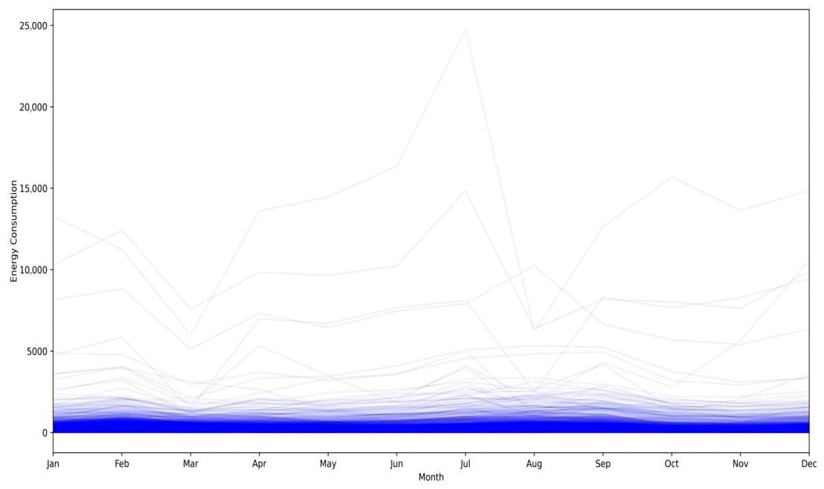
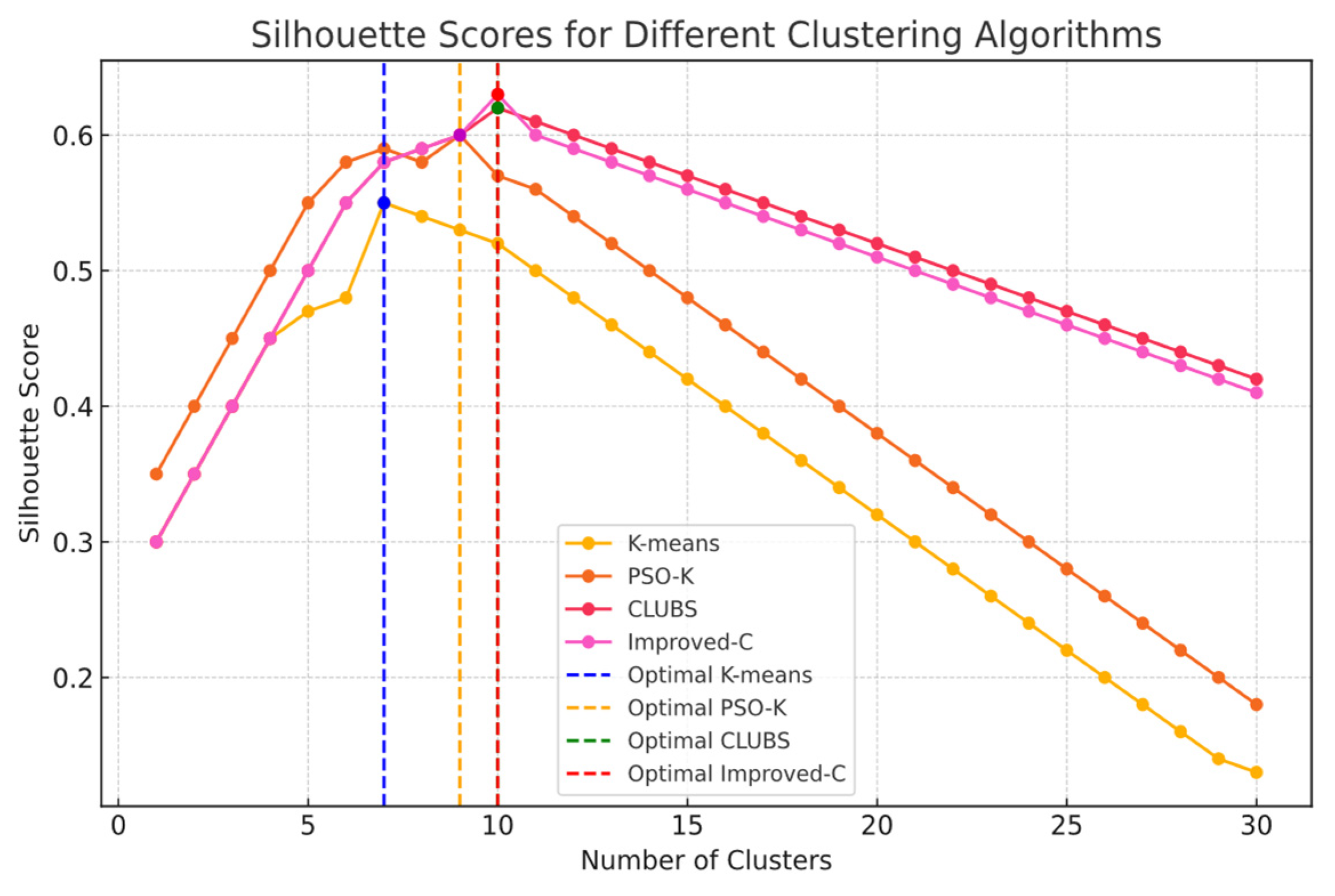
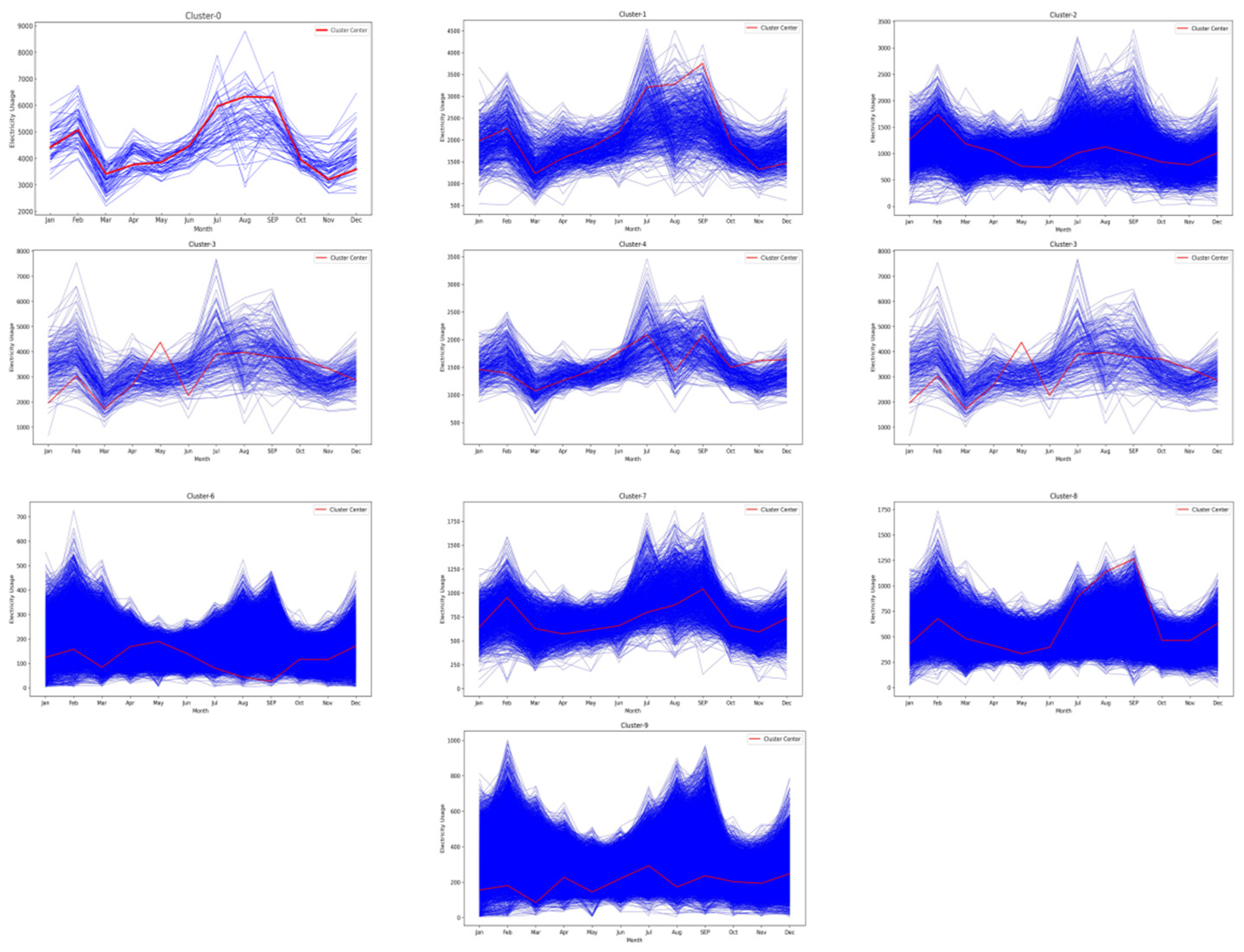
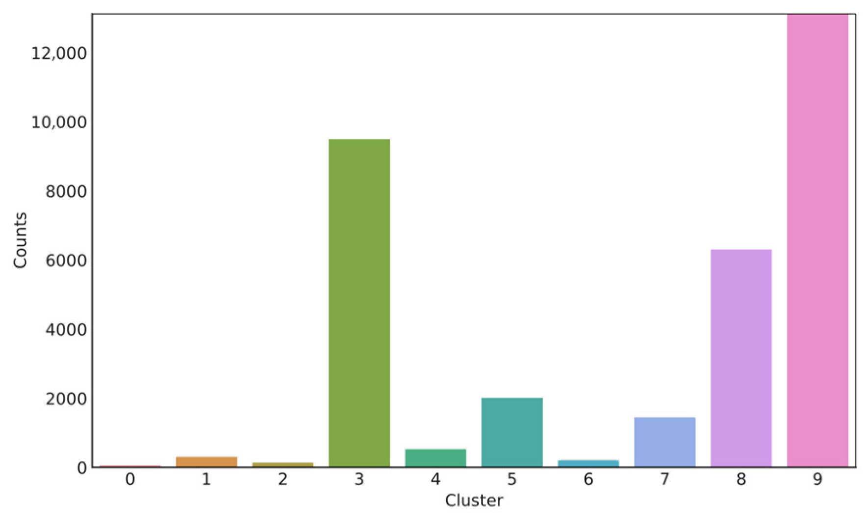
4.1. Clustering for Electricity Consumption Data

The threshold for the cosine similarity filter was set empirically at 0.8 to remove irrelevant window subsequences, balancing computational efficiency and sequence alignment accuracy. The CH index was adopted to guide the splitting process. Splitting continued until the CH index decreases below 70% of its previous value, which ensured robust cluster formation while avoiding over-segmentation. Optimal clusters were determined by the silhouette index.

The Improved-C algorithm was utilized for clustering and analyzing time-series data on user electricity usage. We performed an evaluation of the standard K-means algorithm, the PSO-based K-means algorithm (PSO-K), and the CLUBS algorithm using the silhouette index (SI).

The silhouette index (SI), also known as the silhouette coefficient, is a metric utilized for evaluating the effectiveness of clustering. It assesses cluster compactness and distinction by examining intra-cluster cohesion and inter-cluster separation. The formula for SI is as follows:

$$SI\left(i\right)={\displaystyle \frac{b\left(i\right)-a\left(i\right)}{max\left(a\left(i\right),b\left(i\right)\right)}}$$

(29)

where $a\left(i\right)$ denotes the mean distance of sample $i$ to other samples within the same cluster (mean intra-cluster distance), and $b\left(i\right)$ represents the average distance from sample $i$ to all samples in another specific cluster, where the cluster with the smallest distance is considered the “neighboring cluster” of sample $i$. Depending on the $\mathrm{SI}\left(\mathrm{i}\right)$, the silhouette index of the entire dataset is the mean of the silhouette coefficients of all the samples. The nearer the SI is to 1, the more effective the clustering result is; the closer the SI is to 0, the poorer the clustering outcome is; when a negative value appears, it indicates that the clustering outcome is very bad.

According to the silhouette scores, shown in Figure 9, the optimal numbers of clusters for Improved-C, CLUBS, K-means, and PSO-K are 10, 10, 7, and 9, respectively.

The results are shown in

Table 1. Comparison of three clustering models.

Model	SI	Time(s)
K-means	0.55	125
PSO-K	0.60	306
CLUBS	0.62	102
Improved-C	0.63	115

.

The outcomes indicate that, compared to the standard K-means, PSO-K, and CLUBS clustering methods, the Improved-C algorithm has obvious advantages in terms of theclustering effect, but only a small loss of efficiency, demonstrating the superiority of the improved algorithm.

In addition to the previous plots, Figure 10 shows a comprehensive visualization of all clusters, each of which is shown in a separate subplot. This combined representation offers a comprehensive view of the clustering results, providing a deeper understanding of each cluster. In addition, the cluster center containing each cluster feature further improves the interpretability of the clustering. A histogram search for the number of users per electricity consumption pattern was conducted to examine the characteristics of the ten clusters (Figure 11).

The clustered electricity consumption pattern labels were combined with the original data and user information to generate a new electricity consumption characteristic dataset. The same electricity consumption pattern can be characterized by centroid data, as shown in

Table 2. Electricity consumption characteristic dataset.

JLDBH	YHBH	Jan	Feb	Mar	…	Nov	Dec	Pat
4013XX	4014XX	4529.73	5195.29	3183.92	…	3573.03	4211.42	0
4013XX	4014XX	1468.26	1697.26	1115.15	…	1215.15	1390.69	1
4013XX	4014XX	2553.65	2876.26	1794.82	….	2117.70	2414.48	2
4013XX	4014XX	181.69	233.27	192.47	…	129.21	167.91	3
4013XX	4014XX	1839.56	2149.62	1375.06	…	1554.40	1790.82	4

(partial data). It can be seen that different categories show differentiated electricity consumption behavior. For the same category, the electricity consumption increases significantly in winter and summer due to the influence of season.

4.2. Matching Electricity Consumption Patterns for New Customers

This experiment aims to verify the effectiveness of the DistilBERT-based model in the task of user electricity consumption classification. Firstly, we used the above clustered labeled dataset for DistilBERT fine-tuning to build a downstream classification task model. Then, 15,000 new sample data points were selected from measurements that were not included in the aforementioned cluster analysis. Following data preprocessing, a test dataset for the classification model was created. Given the need to assess the classification performance of DistilBERT, the sampling period and user type of the test sample were known in this instance.

In this paper, the pre-trained DistillBERT encoder was used with a six-layer Transformer encoder with 66 million parameters and a model size of 768. The initial parameters of the DistillBERT model are presented in

Table 3. DistillBERT parameters.

Parameter Name	Default Value
vocab_size	30,522
max_position_embeddings	512
num_attention_heads	12
num_hidden_layers	6
hidden_size	768
intermediate_size	3072
hidden_act	sigmoid
Batch Size	32
Initial Learning Rate	0.001
Epochs	50
Dropout	0.1

.

The classification of user electricity consumption behaviors was derived from a labeled dataset. The variation in classification accuracy was observed as network experiments with different initial learning rates and iteration counts, as depicted in Figure 12. Specifically, when set at an initial learning rate of 0.001, and a cycle count of 50 iterations, the loss trajectories for both the training and testing datasets demonstrate a convergence towards zero, indicating the completion of model training, as illustrated in Figure 13.

To further validate the effectiveness of the DistillBERT algorithms, we compared DistillBERT with baselines, including classical classification models and deep learning models. The results from each algorithm were recorded and compared with the annotated labels, and the accuracy, precision, recall, and F1 score for each algorithm were calculated.

$$\mathrm{Precision}={\displaystyle \frac{\mathrm{TP}}{\mathrm{TP}+\mathrm{FP}}}$$

(30)

$$\mathrm{Recall}={\displaystyle \frac{\mathrm{TP}}{\mathrm{TP}+\mathrm{FN}}}$$

(31)

$$\mathrm{F}1=2·{\displaystyle \frac{\mathrm{precison}\times \mathrm{recall}}{\mathrm{precision}+\mathrm{recall}}}$$

(32)

where TP stands for the number of true positives (accurate matches), FP indicates the number of false positives (incorrect matches), and FN denotes the count of false negatives (the number of unmatched matches that actually should have been matched).

The evaluation values of KNN, SVM, CNN, LSTM, Transformer, and other partial classification models were compared. The comparative results are presented in

Table 4. Assessment of performance across various classifiers.

Model	Accuracy (%)	Precision (%)	Recall (%)	F1 (%)
KNN	81.45	82.32	80.48	81.39
SVM	86.73	87.26	85.91	86.58
CNN	88.47	88.92	87.69	88.30
LSTM	90.28	90.84	89.87	90.35
Transformer	92.13	92.51	91.83	92.17
Shapelet Transform Transform Pipeline	89.50	90.00	88.75	89.37
Fuzzy C-Means + SVM	87.00	87.50	86.25	86.87
DistillBERT	94.21	94.63	94.05	94.34

.

From the above analysis, it can be concluded that DistilBERT and Improved-C clustering can not only assign cluster labels to complex and irregular original electricity data, but also automatically categorize the electricity characteristics of new users, enabling us to analyze users’ electricity behavior according to the existing large-scale power big data.

The algorithm in this paper has been applied in a local power grid to help the electric power company to quickly classify users’ electricity consumption patterns and achieve electricity consumption pattern matching for new users. Utilizing BERT, the power company can promptly identify the power usage behavior of new users and provide personalized power usage suggestions, which significantly improves user satisfaction and grid operation efficiency.

To verify that the improvements in the proposed DistilBERT model are statistically significant compared to other baselines, we conducted paired t-tests based on 10 independent runs for each model (using different random seeds). The means and standard deviations of each metric are shown in

Table 5. Statistical significance test (paired t-test) between DistilBERT and Transformer.

Metric	DistilBERT Mean (Std)	Transformer Mean (Std)	p-Value
Accuracy	94.21 (±0.25)	92.13 (±0.30)	0.0017
Precision	94.63 (±0.22)	92.51 (±0.28)	0.0012
Recall	94.05 (±0.21)	91.83 (±0.27)	0.0019
F1-score	94.34 (±0.20)	92.17 (±0.25)	0.0014

All p-values are less than 0.05, indicating that the improvements achieved by DistilBERT over Transformer are statistically significant at the 95% confidence level.

. We further calculated the p-values for the performance comparisons between DistilBERT and the best-performing baseline (Transformer).

4.3. Ablation Study

To validate the contribution of each key component in the CLB-BER model, we conducted ablation experiments isolating the effects of the ECDW enhancement in CLUBS clustering and DistilBERT fine-tuning for classification.

First, we ablated the ECDW method from the Improved-C (CLUBS) clustering phase, reverting to the standard CLUBS algorithm while keeping the downstream DistilBERT classification intact. As shown in

Table 6. Ablation study results.

Variant	SI	Accuracy (%)	F1 (%)
Full CLB-BER (Improved-C+DistilBERT)	0.63	94.21	94.34
Without ECDW (CLUBS + DistilBERT)	0.62	92.50	92.75
Improved-C+ SVM	-	86.73	86.58
Improved-C+LSTM	-	90.28	90.35

, without ECDW, the silhouette index (SI) drops from 0.63 to 0.62 (consistent with the baseline CLUBS performance in Table 1), indicating reduced clustering quality due to the poorer handling of sequence misalignment and temporal symmetry. This propagates to downstream classification, reducing the accuracy from 94.21% to 92.50%, as the less-accurate cluster labels degrade the fine-tuning process.

Second, we replace the fine-tuned DistilBERT with alternative classifiers (SVM and LSTM) while retaining the Improved-C clustering labels for training. This isolates the benefit of DistilBERT’s contextual representation learning over simpler models. The results in Table 5 show that SVM achieves 86.73% accuracy (a 7.48% drop from the full model), and LSTM reaches 90.28% (a 3.93% drop), highlighting DistilBERT’s superiority in capturing complex temporal patterns in electricity data.

5. Conclusions

To overcome data challenges, enhance technology portability, and prevent redundant investments, this study presents an LLM-based application framework integrating three key scenarios: load prediction and optimization, equipment anomaly detection with predictive maintenance, and power system security with data privacy. This framework shows promising applications for multi-source, heterogeneous, and massive data in modern power systems.

Based on our LLM framework, we developed CLB-BER to address the core challenge of electricity consumption behavior analysis. The ECDW method optimizes the CLUBS algorithm’s adjustment stage, enabling the accurate classification of consumption patterns and mapping between unlabeled behavior characteristics and user types. Our pre-trained BERT model predicts user types from new consumption data, enabling personalized strategies and intelligent load scheduling, overcoming the limitations of conventional single-analysis methods. By preserving temporal symmetry in consumption patterns, our approach achieves higher generalization across heterogeneous grid scenarios.

Evaluations on real grid datasets demonstrate that our enhanced CLUBS algorithm significantly improves clustering precision. Compared to direct neural network training with raw data, our approach reduces computation time while increasing classification accuracy for new electricity data, providing valuable insights for targeted utility marketing strategies.

This study has limitations worth noting. The experimental evaluation was conducted on electricity consumption data from a single local grid spanning only one year (2019). Thus, the generalizability of our approach across different geographic regions or extended time periods remains to be further validated. Future studies should aim to apply the proposed CLB-BER model to datasets from multiple power grids and diverse climatic regions, as well as perform longitudinal analyses over several consecutive years. More advanced LLM algorithms must be integrated for equipment fault diagnosis, predictive maintenance, and power system security. Future work will expand the system to accommodate various power system neighborhoods, addressing a wider range of practical challenges in the evolving energy landscape.

References

1. Wang, H.; Yi, Z.; Xu, Y.; Cai, Q.; Li, Z.; Wang, H.; Bai, X. Data-driven distributionally robust optimization approach for the coordinated dispatching of the power system considering the correlation of wind power. Electr. Power Syst. Res. 2024, 230, 110224. [Google Scholar] [CrossRef]
2. Li, G.; Wang, K.; Lin, Y.; Lu, T.; Li, Y.; Han, F. Fault Diagnosis and Prediction Method of Distribution Transformer in Active Distribution Network Based on Data Augmentation. In Proceedings of the 2023 3rd International Conference on Electrical Engineering and Mechatronics Technology (ICEEMT), Nanjing, China, 21–23 July 2023; IEEE: New York, NY, USA, 2023; pp. 137–141. [Google Scholar]
3. Huang, J.; Wu, F.; Li, Y.; Qian, J.; Yang, Y.; Yao, W. Safety analysis of new power system based on graph convolutional neural network evaluation. In Proceedings of the 2023 10th International Forum on Electrical Engineering and Automation (IFEEA), Nanjing, China, 3–5 November 2023; IEEE: New York, NY, USA, 2023; pp. 1188–1192. [Google Scholar]
4. Liu, Z.; Hu, C.; Xia, H.; Xiang, T.; Wang, B.; Chen, J. SPDTS: A Differential Privacy-Based Blockchain Scheme for Secure Power Data Trading. IEEE Trans. Netw. Serv. Manag. 2022, 19, 5196–5207. [Google Scholar] [CrossRef]
5. Vaswani, A.; Shazeer, N.; Parmar, N.; Uszkoreit, J.; Jones, L.; Gomez, A.N.; Kaiser, L.; Polosukhin, I. Attention Is All You Need. arXiv 2017, arXiv:1706.03762. [Google Scholar]
6. Yang, J.; Jin, H.; Tang, R.; Han, X.; Feng, Q.; Jiang, H.; Yin, B.; Hu, X. Harnessing the Power of LLMs in Practice: A Survey on ChatGPT and Beyond. arXiv 2023, arXiv:2304.13712. [Google Scholar] [CrossRef]
7. Zhao, W.X.; Zhou, K.; Li, J.; Tang, T.; Wang, X.; Hou, Y.; Min, Y.; Zhang, B.; Zhang, J.; Dong, Z.; et al. A Survey of Large Language Models. arXiv 2023, arXiv:2303.18223. [Google Scholar] [PubMed]
8. Shakarian, P.; Koyyalamudi, A.; Ngu, N.; Mareedu, L. An Independent Evaluation of ChatGPT on Mathematical Word Problems (MWP). arXiv 2023, arXiv:2302.13814. [Google Scholar] [CrossRef]
9. Gruver, N.; Finzi, M.; Stanton, S.; Wilson, A.G. Time Series Forecasting by Reprogramming Large Language Models. In ICLR 2024, Vienna, Austria, 7 May 2024; OpenReview: Alameda, CA, USA; Available online: https://openreview.net/forum?id=Unb5CVPtae (accessed on 16 January 2024).
10. Jin, M.; Wen, S.; Song, Y.; Paik, H.Y. Empowering Time Series Analysis with Large Language Models. In Proceedings of the 33rd International Joint Conference on Artificial Intelligence (IJCAI), Jeju, Republic of Korea, 3–9 August 2024; IJCAI: Jeju, Republic of Korea, 2024; Available online: https://www.ijcai.org/proceedings/2024/0895.pdf (accessed on 11 April 2024).
11. Zhou, T.; Ma, Z.; Wen, Q.; Wang, X.; Sun, L.; Jin, R. Are Language Models Actually Useful for Time Series Forecasting? In Proceedings of the 38th Conference on Neural Information Processing Systems (NeurIPS), Vancouver, BC, Canada, 9–15 December 2024; Available online: https://proceedings.neurips.cc/paper_files/paper/2024/file/6ed5bf446f59e2c6646d23058c86424b-Paper-Conference.pdf (accessed on 15 April 2024).
12. Xue, H.; Li, Y.; Zhang, J.; Chen, L. A large language model for advanced power dispatch. Sci. Rep. 2025, 15, 91940. [Google Scholar] [CrossRef] [PubMed]
13. Liu, Z.; Zhang, W.; Li, H. Are Large Language Models Useful for Time Series Data Analysis? arXiv 2024, arXiv:2412.12219. [Google Scholar] [CrossRef]
14. Feng, S.Y.; Gangal, V.; Wei, J.; Chandar, S.; Vosoughi, S.; Mitamura, T.; Hovy, E. A survey of data augmentation approaches for NLP. arXiv 2021, arXiv:2105.03075. [Google Scholar] [CrossRef]
15. Novelli, C.; Casolari, F.; Rotolo, A.; Taddeo, M.; Floridi, L. Taking AI risks seriously: A new assessment model for the AI act. AI Soc. 2024, 39, 2493–2497. [Google Scholar] [CrossRef]
16. Cai, Y.; Mao, S.; Wu, W.; Wang, Z.; Liang, Y.; Ge, T.; Wu, C.; You, W.; Song, T.; Xia, Y. Low-code LLM: Visual programming over LLMs. arXiv 2023, arXiv:2304.08103. [Google Scholar]
17. Jain, R.; Gervasoni, N.; Ndhlovu, M.; Rawat, S. A code centric evaluation of C/C++ vulnerability datasets for deep learning based vulnerability detection techniques. In Proceedings of the 16th Innovations in Software Engineering Conference, Allahabad, India, 23–25 February 2023; ACM: New York, NY, USA, 2023; pp. 1–10. [Google Scholar]
18. Thirunavukarasu, A.J.; Ting, D.S.J.; Elangovan, K.; Gutierrez, L.; Tan, T.F.; Ting, D.S.W. Large language models in medicine. Nat. Med. 2023, 29, 1930–1940. [Google Scholar] [CrossRef] [PubMed]
19. Arcila, B.B. Is it a platform? Is it a search engine? It’s ChatGPT! the European liability regime for large language models. J. Free. Speech Law 2023, 3, 455. [Google Scholar]
20. OpenAI. GPT-4 technical report. arXiv 2023, arXiv:2303.08774. [Google Scholar] [CrossRef]
21. Anthropic. (n.d.). Introducing Claude. Available online: https://www.anthropic.com/index/introducing-claude (accessed on 17 June 2025).
22. Roziere, B.; Gehring, J.; Gloeckle, F.; Sootla, S.; Gat, I.; Tan, X.E.; Adi, Y.; Liu, J.; Remez, T.; Rapin, J. Code llama: Open foundation models for code. arXiv 2023, arXiv:2308.12950. [Google Scholar]
23. Taori, R.; Gulrajani, I.; Zhang, T.; Dubois, Y.; Li, X.; Guestrin, C.; Liang, P.; Hashimoto, T.B. Alpaca: A Strong, Replicable Instruction-Following Model. Available online: https://crfm.stanford.edu/2023/03/13/alpaca.html (accessed on 20 April 2024).
24. Wolf, T.; Debut, L.; Sanh, V.; Chaumond, J.; Delangue, C.; Moi, A.; Cistac, P.; Rault, T.; Louf, R.; Funtowicz, M.; et al. HuggingFace’s transformers: State-of-the-art natural language processing. arXiv 2020, arXiv:1910.03771. [Google Scholar]
25. Ianni, M.; Masciari, E.; Mazzeo, G.M.; Mezzanzanica, M.; Zaniolo, C. Fast and effective Big Data exploration by clustering. Future Gener. Comput. Syst. 2020, 102, 84–94. [Google Scholar] [CrossRef]
26. Savci, P.; Das, B. Comparison of pre-trained language models in terms of carbon emissions, time and accuracy in multi-label text classification using AutoML. Heliyon 2023, 9, e15670. [Google Scholar] [CrossRef] [PubMed]
27. Devlin, J.; Chang, M.-W.; Lee, K.; Toutanova, K. BERT: Pre-training of deep bidirectional transformers for language understanding. arXiv 2018, arXiv:1810.04805. [Google Scholar]
28. Alammary, A.S. BERT models for Arabic text classification: A systematic review. Appl. Sci. 2022, 12, 5720. [Google Scholar] [CrossRef]
29. Du, X.; Liu, Z.; Li, C.; Ma, X.; Li, Y.; Wang, X. LLM-BRC: A large language model-based bug report classification framework. Softw. Qual. J. 2024, 32, 985–1005. [Google Scholar] [CrossRef]
Figure 1. BERT network input and coding.
Symmetry 17 01176 g001
Figure 2. Application framework based on LLMs.
Symmetry 17 01176 g002
Figure 3. Model framework for classifying electricity consumption behavior.
Symmetry 17 01176 g003
Figure 4. Data processing flow chart.
Symmetry 17 01176 g004
Figure 5. Improved-C algorithm flow.
Symmetry 17 01176 g005
Figure 6. A block containing a cluster (a) and a block containing only outliers (b).
Symmetry 17 01176 g006
Figure 7. DistilBERT classification model.
Symmetry 17 01176 g007
Figure 8. Data visualization.
Symmetry 17 01176 g008
Figure 9. SI scores for clusters and algorithm.
Symmetry 17 01176 g009
Figure 10. Visualization of typical electricity usage patterns.
Symmetry 17 01176 g010
Figure 11. Histogram of the cluster.
Symmetry 17 01176 g011
Figure 12. Variability in accuracy across different learning rates.
Symmetry 17 01176 g012
Figure 13. Training set loss function curve.
Symmetry 17 01176 g013