Algorithm to Find and Analyze All Configurations of Four-Bar Linkages with Different Geometric Loci Degenerate Forms

Abstract

A general algorithm to determine the coupler link geometric loci, such as centrodes, inflection and return circles, as well as circling-point and centering-point curves, is formulated to analyze any type of four-bar linkages with the main target to find all mechanism configurations, in which at least one of the above-mentioned loci degenerates. Thus, different types of four-bar linkages, such as crank-rocker, double-crank, double-rocker and triple-rocker, are classified according to Grashof’s law, in order to distinguish and analyze their corresponding geometric loci. In particular, the proposed algorithm is based on four diagrams of the angular velocity ratios versus the mechanism driving angle, which consider the links pairs of input/output, input/coupler, and output/coupler, along with those of coupler/input and coupler/output for their relative motion. These diagrams allow the determination of all mechanism configurations according to Freudenstein’s theorems, where the aforementioned geometric loci degenerate into straight lines, including the line at infinity, ϕ-curves, and/or equilateral hyperbolas. This algorithm has been implemented in Matlab in order to run several examples regarding different four-bar linkages, according to Grashof’s law, and analyzing the degenerate forms of their inflection and return circles, as well as the circling-point and centering-point curves, that are also validated by using the collineation axis.

1. Introduction

Four-bar linkages represent one of the most widely studied planar mechanical systems due to their simplicity, versatility, and relevance in motion generation and control. Their structure, consisting of four rigid bodies connected by four revolute joints, forms the foundation of many motion-generating mechanisms used in robotics, industrial automation, and biomechanical devices. The analysis of such systems relies heavily on the geometric and algebraic relationships among the link parameters and their relative motions, with a particular focus on configurations that lead to critical kinematic behaviors. Among the analytical key tools for understanding 4R linkages, there are the classical theorems introduced by Freudenstein, which formalize the input–output angular relationships and provide a systematic basis for evaluating velocity and acceleration characteristics. In particular, the work in [1] established geometrical criteria to detect maximum and minimum angular velocity ratios and compute accelerations in specific configurations, laying the foundation for velocity-based mechanism design. A reformulation of these theorems using vector loop equations was proposed in [2], where the authors demonstrated how different analytical forms could be used to identify phases of extreme motion while also clarifying the limitations in locating exact configuration values. The formal structure of Freudenstein’s relationships has been the subject of further refinement, including purely vectorial derivations [3], which reinforce their algebraic transparency and value. More recently, in [4] is a differential algebraic framework that extends the traditional formulation to higher-order derivatives of input–output equations, enabling the evaluation of signed velocity ratios and acceleration conditions across six possible angular configurations, is proposed. This approach not only enriches the interpretation of Freudenstein’s results but also connects them to more advanced studies on force transmission and dynamic response. In parallel, the geometric implications of Freudenstein-like conditions have been explored in [5], where the authors investigated symmetrical coupler curves designed to approximate straight-line paths. By exploiting the collinearity of Burmester points, they demonstrated how certain degenerate conditions can be purposefully designed using extended Freudenstein-based criteria.

While the classical kinematic framework offers a solid basis for analyzing general motion in 4R mechanisms, particular attention must be given to those configurations in which the behavior of the system becomes critical or degenerate. These configurations, typically referred to as singularities or asymptotic configurations, are of great importance in both theoretical analysis and practical design, as they often correspond to sudden changes in mobility, loss of control, or degeneration of characteristic geometric loci. Understanding and predicting such behaviors is therefore essential when aiming for reliable and robust mechanical performance. One early contribution to this area is the graphical method proposed in [6], which simplifies the acceleration analysis of four-bar linkages without relying on velocity or acceleration polygons, providing a faster and more intuitive assessment of follower behavior near critical configurations. Degenerate forms of specific geometric loci were studied in [7], where a four-bar linkage was used to drive a Geneva wheel with jerk-free motion. Here, the authors observed how the coupler-point path could collapse into symmetrical forms, depending on the linkage parameters. A more systematic classification of such degeneracies was later developed in [8], where conditions for the degeneration of circling-point and centering-point curves were established analytically, and presented in a compact tabular format. The higher-order analysis of such phenomena has been extended through screw theory and curvature methods. In [9], the authors presented a framework for evaluating the stationary curvature properties of four-bar mechanisms using derivatives of screws, revealing how classical loci such as the cubic of stationary curvature behave in translational and rotational configurations. Furthermore, they showed that traditional coordinate-based methods fail in certain geometries, such as parallelogram linkages, which can instead be treated effectively using screw-based tools. Similarly, in [10], screw system algebra is applied to analyze uncertainty configurations, extending these techniques to both planar and spatial chains, and demonstrating their applicability to the detection of limiting behavior in higher-degree mechanisms. Analytical insights into singular configurations were also offered in [11], where the authors categorized the singularities of closed-loop kinematic chains through the properties of the Jacobian matrices, providing a classification that is widely applicable to both linkages and parallel robots. Geometric consequences of these singularities were further explored in [12], which examined the behavior of coupler-point paths and line envelopes as the instantaneous center approaches infinity, revealing characteristic degenerations in the inflection and cusp circles. A complementary approach was presented in [13], which introduced improved definitions for circuits and branches in planar mechanisms and emphasized how topological ambiguities may conceal degenerate conditions. More complex configurations were examined in [14], where double configurations in Assur kinematic chains and stationary states in Stephenson six-bar linkages were analyzed through the gradient of the coupler curve and its relation to dismantled binary links. Several studies have focused specifically on dead-center positions, where the mechanism temporarily loses mobility. The modular analysis method proposed in [15] uses Assur kinematic chains to identify these positions based on the gain of mobility in substructures. A related polynomial-based method was introduced in [16], which formulates necessary conditions for dead-center states in Stephenson six-bar linkages using Sturm functions and input–output equations. Earlier treatments of this problem include [17,18], which applied instant center methods and kinematic inversion to map all possible stationary configurations in six-bar planar mechanisms. The consequences of such configurations on practical mechanism design are non-trivial. For instance, in [19], the instantaneous motion of a line in asymptotic positions was investigated, showing how centrodes behave near an infinite pole and how line-envelope contact points change their nature in such cases. These results highlight the need to consider higher-order effects when approaching degeneracies. Recent contributions have also integrated these concepts into kinematic synthesis procedures. In [20], the authors proposed a method for generating Stephenson III six-bar mechanisms with instantaneous stop in the coupler link, combining a crank-driven, four-bar sub-chain with a ternary coupler link specifically configured to exhibit an instantaneous stop. In [21], the same class of mechanisms was studied in terms of first- and second-order centrodes, with particular attention to cases where the coupler exhibits an instantaneous stop and/or a simple dwell. The study of geometric loci in planar mechanisms represents a key aspect of kinematic analysis and synthesis. These loci are crucial for understanding the qualitative behavior of mechanisms and for guiding the design, for example, of paths with desired curvature, shape, or functional properties. Among the most significant loci are the centrodes, the inflection circle, the return circle, the cubic of stationary curvature, and the circling-point and centering-point curves. Their characterization provides essential insights into transmission efficiency, instantaneous kinematic properties, and critical configurations. The synthesis of mechanisms aimed at producing quasi-constant transmission ratios often relies on the precise control of such loci. In [22], closed-form algorithms were developed to design planar linkages, both four-bar and slider–crank types, with prescribed curvature behavior. By combining centrode analysis, inflection circles, and the Euler–Savary equation, the authors demonstrated how to obtain consistent motion profiles across infinitesimal and finite displacements. An example of kinematic modeling and synthesis applied to more complex mechanical systems can be found in [23], where an eight-bar mechanism was proposed for an upper-limb exoskeleton aimed at assisting elbow joint motion during repetitive heavy-lifting tasks [23]. The nature of higher-order loci was further investigated in [24], where algorithms for computing first-, second-, and third-order centrodes as well as Bresse’s circles were proposed. These allow for the visualization of instantaneous centers of rotation, acceleration, and jerk across a wide range of configurations, showing how such higher-order information can inform mechanism design at a deeper level. Other geometric curves with relevance to planar kinematics have also been explored. In [25], the mathematical properties of strophoids were discussed in detail. These curves emerge naturally as projections of circle-point curves, and exhibit numerous geometric symmetries and involutions, which can be exploited in the design of mechanisms with stationary curvature features. Foundational treatments of motion geometry can be found in classic texts such as [26,27], which provide comprehensive formulations of linkage motion and coupler curve generation. These works laid the groundwork for later developments in the synthesis and classification of mechanism behavior. Similarly, ref. [28] offers a modern reinterpretation of curvature theory in planar motion, with a particular emphasis on instantaneous invariants and their role in guiding motion synthesis. Other key references that consolidate the theoretical basis of geometric loci analysis include [29], where the Carter-Hall circle is defined via velocity diagrams and used for the synthesis of fifth-order function generators, and [30], which presents a geometric method to coordinate coupler-point positions and crank rotations based on Roberts’ configuration. The synthesis of paths with desired directionality and timing is addressed through Burmester curves and degenerate forms of coupler motion. Comprehensive introductions to these concepts are also provided in classical textbooks such as [31,32,33,34], which collectively address the geometry of planar mechanisms, the kinematic synthesis of linkages, and the role of curvature and centrodes in practical design scenarios. Complementary to the analytical and geometric methods discussed above, recent studies in the field of robotics have explored the use of intelligent and adaptive strategies to deal with critical configurations and motion planning in complex environments. Such approaches often rely on evolutionary algorithms and data-driven models to enhance system robustness under degenerate or uncertain conditions [35,36].

In this paper, a general algorithm to find and analyze all configurations of four-bar linkages with different geometric loci degenerate forms, is proposed. In fact, as reported above, in the state-of-the-art analysis, there is not any scientific paper dealing with this specific topic, as the simplification of the design process of path generators and dwell mechanisms. In particular, different types of four-bar linkages are classified according to Grashof’s law, while four diagrams of the angular–velocity ratios versus the mechanism driving angle are determined to identify, in agreement with Freudenstein’s theorems, the four-bar linkages configurations, where the above-mentioned geometric loci degenerate into straight lines, including the line at infinity, ϕ-curves, and/or equilateral hyperbolas. This algorithm has been implemented in Matlab and validated by using the collineation axis and several significant examples.

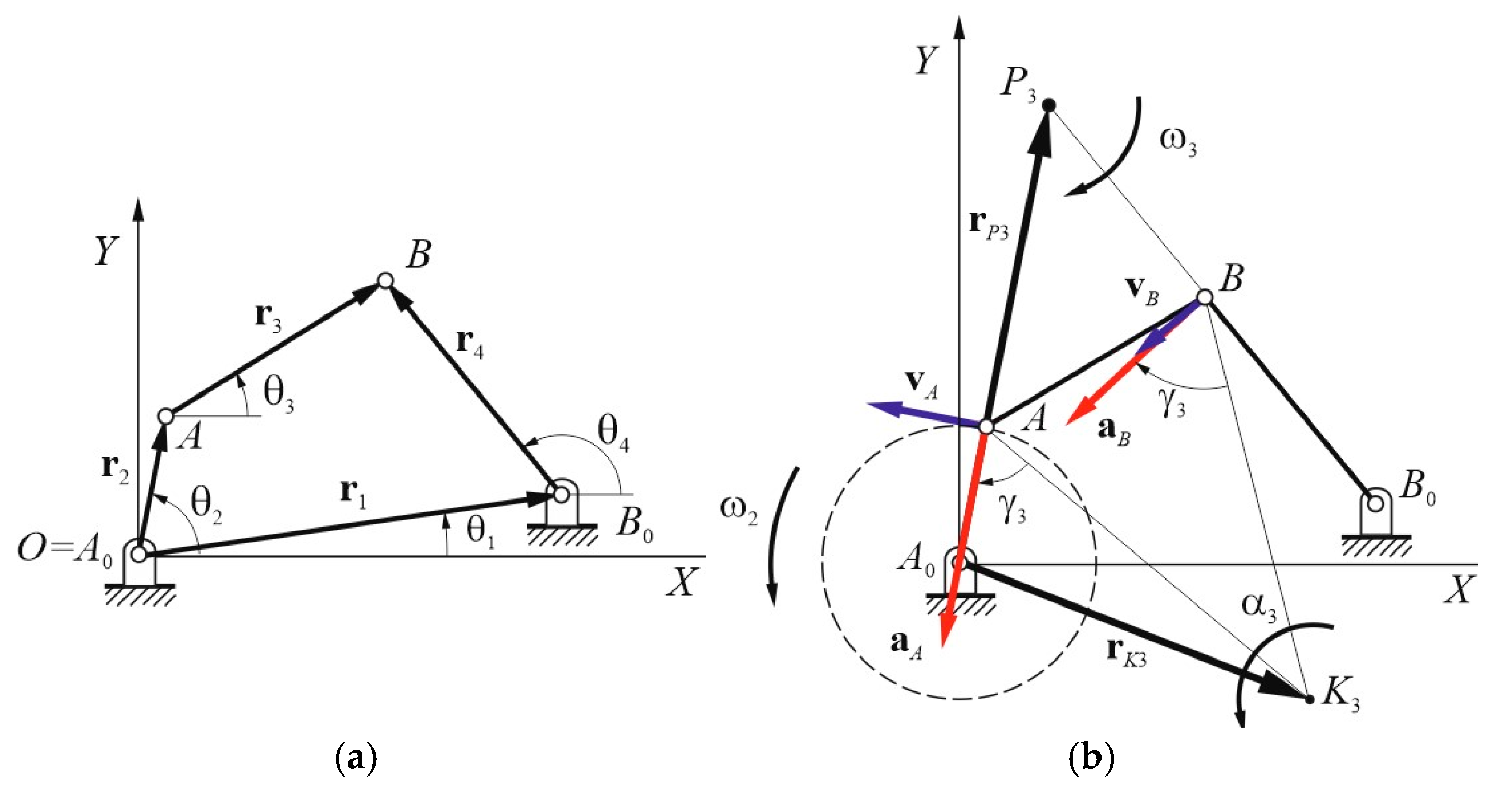
2. Kinematic Analysis: Velocity and Acceleration Poles

This section deals with the kinematic analysis of four-bar mechanisms, focusing on Grashof’s law, different inversions, and position analysis.

Grashof’s law determines the rotational behavior of linkages in a planar four-bar mechanism. It states that, for a continuous relative rotation between two elements, the sum of the lengths of the shortest link s and the longest link l must be less than or equal to the sum of the lengths of the other two links, p and q. This is expressed as

$$s+l\le p+q$$

(1)

A four-bar chain that satisfies the Grashof inequality is referred to as a Grashof chain. In such a mechanism, the shortest link s is always capable of continuous rotation relative to the other three links. The type of motion produced by a Grashof chain depends on which link is fixed. If the link adjacent to the shortest link is fixed, the mechanism functions as a crank-rocker, where the s acts as the crank and rotates continuously, while its opposite link oscillates and serves as the rocker. When the s itself is fixed, the mechanism becomes a double-crank linkage, allowing both adjacent links to fully rotate, with the shorter of the two typically designated as the input crank. Alternatively, if the link opposite to the shortest one is fixed, the mechanism becomes a double-rocker, in which neither of the adjacent links can complete a full rotation, and both merely oscillate. If the Grashof inequality is not satisfied, the mechanism is classified as a non-Grashof chain. In this case, no single link is capable of a complete revolution regardless of which link is fixed. The only possible inversion in a non-Grashof configuration is the triple-rocker mechanism, where all three moving links are restricted to oscillatory motion.

Referring to the kinematic sketch of Figure 1, the position analysis of a generic four-bar mechanism can be determined through the following loop-closure equation:

$${\mathbf{r}}_2+{\mathbf{r}}_3={\mathbf{r}}_1+{\mathbf{r}}_4$$

(2)

where r_i represents the position vector for link i (for i = 1, …, 4). These position vectors can be expressed in vector form with respect to the fixed frame OXY, as follows:

$${\mathbf{r}}_i=r_i\left(\mathrm{c}\mathrm{o}\mathrm{s}{\theta }_i\mathbf{i}+\mathrm{s}\mathrm{i}\mathrm{n}{\theta }_i\mathbf{j}\right)$$

(3)

where r_i denotes the magnitude and θ_i represents the counterclockwise-oriented angle of position vector r_i. Specifically, θ₂ represents the driving angle of the input link 2. For the fixed link 1, r₁ and θ₁ are constant values representing the magnitude and orientation from point A₀ to B₀, respectively. The position vectors for specific points, such as r_A and r_B of points A and B, can also be expressed as

$$\begin{gathered} {\mathbf{r}}_A={\mathbf{r}}_2 \\ {\mathbf{r}}_B={\mathbf{r}}_1+{\mathbf{r}}_4 \end{gathered}$$

(4)

Referring to the scheme of Figure 1a, the angular position θ₃ of coupler link AB can be evaluated by developing Equation (2), as follows:

$${\theta }_3={\tan }^{-1}\left({\displaystyle \frac{r_1\sin {\theta }_1-r_2\sin {\theta }_2+r_4\sin {\theta }_4}{r_1\cos {\theta }_1-r_2\cos {\theta }_2+r_4\cos {\theta }_4}}\right)$$

(5)

The angular position θ₄ of link B₀B can be expressed as

$${\theta }_4=2\mathrm{t}\mathrm{a}{\mathrm{n}}^{-1}{\displaystyle \frac{-ℬ+\sigma \sqrt{{ℬ}^2-C^2+{𝒜}^2}}{C-𝒜}}$$

(6)

where σ is equal to ±1 according to a suitable assembly mode and the parameters:

$$\begin{gathered} 𝒜=2r_1{r}_4\cos {\theta }_1-2r_2{r}_4\cos {\theta }_2 \\ ℬ=2r_1{r}_4\mathrm{s}\mathrm{i}\mathrm{n}{\theta }_1-2r_2{r}_4\sin {\theta }_2 \\ C=r_1^2+r_2^2+r_4^2-r_3^2-2r_1{r}_2\cos \left({\theta }_1-{\theta }_2\right) \end{gathered}$$

(7)

By the first-time derivatives of Equation (2), one has the angular velocity vectors ω₃ and ω₄

$${\mathbf{\omega }}_3={\dot{\theta }}_3 \mathbf{k}=\left[{\omega }_2{\displaystyle \frac{r_2}{r_3}}{\displaystyle \frac{\sin \left({\theta }_2-{\theta }_4\right)}{\sin \left({\theta }_4-{\theta }_3\right)}}\right]\mathbf{k}$$

(8)

$${\mathbf{\omega }}_4={\dot{\theta }}_4 \mathbf{k}=\left[{\displaystyle \frac{r_2{\omega }_2}{r_4}}{\displaystyle \frac{\sin \left({\theta }_2-{\theta }_3\right)}{\sin \left({\theta }_4-{\theta }_3\right)}}\right]\mathbf{k}$$

(9)

where ω₂ represents the angular velocity magnitude of the input link 2.

The second-time derivatives of Equation (2) yield the angular acceleration α₃ and α₄ as

$${\mathbf{\alpha }}_3={\ddot{\theta }}_3 \mathbf{k}=\left[{\displaystyle \frac{r_2{\alpha }_2 \mathrm{s}\mathrm{i}\mathrm{n}\left({\theta }_2-{\theta }_4\right)+r_2{\omega }_2^2\mathrm{c}\mathrm{o}\mathrm{s}\left({\theta }_2-{\theta }_4\right)+r_3{\omega }_3^2\mathrm{c}\mathrm{o}\mathrm{s}\left({\theta }_3-{\theta }_4\right)-r_4{\omega }_4^2}{r_3 \mathrm{s}\mathrm{i}\mathrm{n}\left({\theta }_4-{\theta }_3\right)}}\right]\mathbf{k}$$

(10)

$${\mathbf{\alpha }}_4={\ddot{\theta }}_4 \mathbf{k}=\left[{\displaystyle \frac{r_2{\alpha }_2 \mathrm{s}\mathrm{i}\mathrm{n}\left({\theta }_2-{\theta }_3\right)+r_2{\omega }_2^2\mathrm{c}\mathrm{o}\mathrm{s}\left({\theta }_2-{\theta }_3\right)+r_3{\omega }_3^2-r_4{\omega }_4^2\mathrm{c}\mathrm{o}\mathrm{s}\left({\theta }_4-{\theta }_3\right)}{r_4 \mathrm{s}\mathrm{i}\mathrm{n}\left({\theta }_4-{\theta }_3\right)}}\right]\mathbf{k}$$

(11)

where α₂ represents the angular acceleration of input link 2.

Referring to the scheme of Figure 1b, the velocity vectors v_A, v_B, and v_P3 of points A, B, and P₃ can be expressed as

$${\mathbf{v}}_A={\dot{\mathbf{r}}}_2=-\left({\omega }_2{r}_2\sin {\theta }_2\right)\mathbf{i}+\left({\omega }_2{r}_2\cos {\theta }_2\right)\mathbf{j}$$

(12)

$${\mathbf{v}}_B={\dot{\mathbf{r}}}_4={\dot{\mathbf{r}}}_2+{\mathbf{\omega }}_3\times \left({\mathbf{r}}_4-{\mathbf{r}}_2\right)$$

(13)

$${\mathbf{v}}_{P3}={\dot{\mathbf{r}}}_{P3}={\dot{\mathbf{r}}}_2+{\mathbf{\omega }}_3\times \left({\mathbf{r}}_{P3}-{\mathbf{r}}_2\right)$$

(14)

where r_P3 is the position vector of the velocity pole P₃ that can be obtained by Equation (14) by imposing v_P3 = 0, and thus, one has

$${\mathbf{r}}_{P3}=\left(-{\displaystyle \frac{{\dot{r}}_{2y}}{{\omega }_3}}+r_{2x}\right)\mathbf{i}+\left({\displaystyle \frac{{\dot{r}}_{2x}}{{\omega }_3}}+r_{2y}\right)\mathbf{j}$$

(15)

Similarly, the acceleration vectors a_A, a_B, and a_K3 of points A, B, and K₃, respectively, in agreement with the Rivals theorem, take the following expressions:

$${\mathbf{a}}_A={\ddot{\mathbf{r}}}_2=\left(-{\omega }_2^2{r}_2\cos {\theta }_2-{\alpha }_2{r}_2\sin {\theta }_2\right)\mathbf{i}+\left(-{\omega }_2^2{r}_2\sin {\theta }_2+{\alpha }_2{r}_2\cos {\theta }_2\right)\mathbf{j}$$

(16)

$${\mathbf{a}}_B={\ddot{\mathbf{r}}}_4={\ddot{\mathbf{r}}}_2+{\mathbf{\alpha }}_3\times \left({\mathbf{r}}_4-{\mathbf{r}}_2\right)+{\mathbf{\omega }}_3\times \left[{\mathbf{\omega }}_3\times \left({\mathbf{r}}_4-{\mathbf{r}}_2\right)\right]$$

(17)

$${\mathbf{a}}_{K3}={\ddot{\mathbf{r}}}_{K3}={\ddot{\mathbf{r}}}_2+{\mathbf{\alpha }}_3\times \left({\mathbf{r}}_{K3}-{\mathbf{r}}_2\right)+{\mathbf{\omega }}_3\times \left[{\mathbf{\omega }}_3\times \left({\mathbf{r}}_{K3}-{\mathbf{r}}_2\right)\right]$$

(18)

where r_K3 is the position vector of the acceleration pole K₃ that can be derived by Equation (18) for a_K3 = 0, and thus, one has

$${\mathbf{r}}_{K3}=\left({\displaystyle \frac{{\omega }_3^2{\ddot{r}}_{2x}-{\alpha }_3{\ddot{r}}_{2y}}{{\omega }_3^4+{\alpha }_3^2}}+r_{2x}\right)\mathbf{i}+\left({\displaystyle \frac{{\alpha }_3{\ddot{r}}_{2x}+{\omega }_3^2{\ddot{r}}_{2y}}{{\omega }_3^4+{\alpha }_3^2}}+r_{2y}\right)\mathbf{j}$$

(19)

Therefore, the position vectors r_P3 and r_K3 of the velocity P₃ and acceleration K₃ poles are given by Equations (15) and (19), respectively, while the corresponding angular velocity ω₃ and acceleration α₃ vectors are given by Equations (8) and (10).

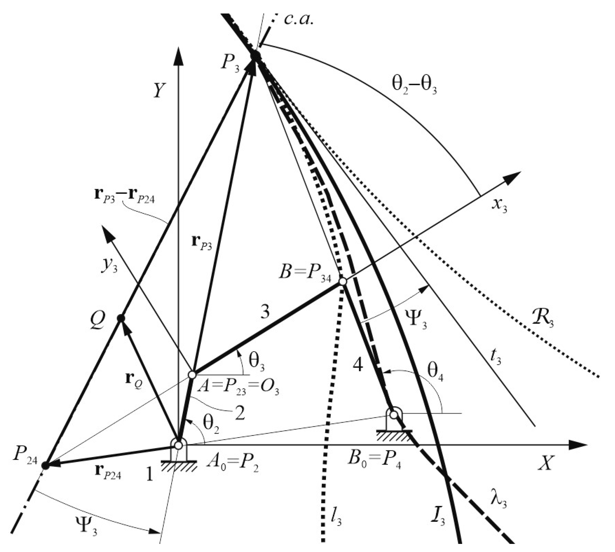
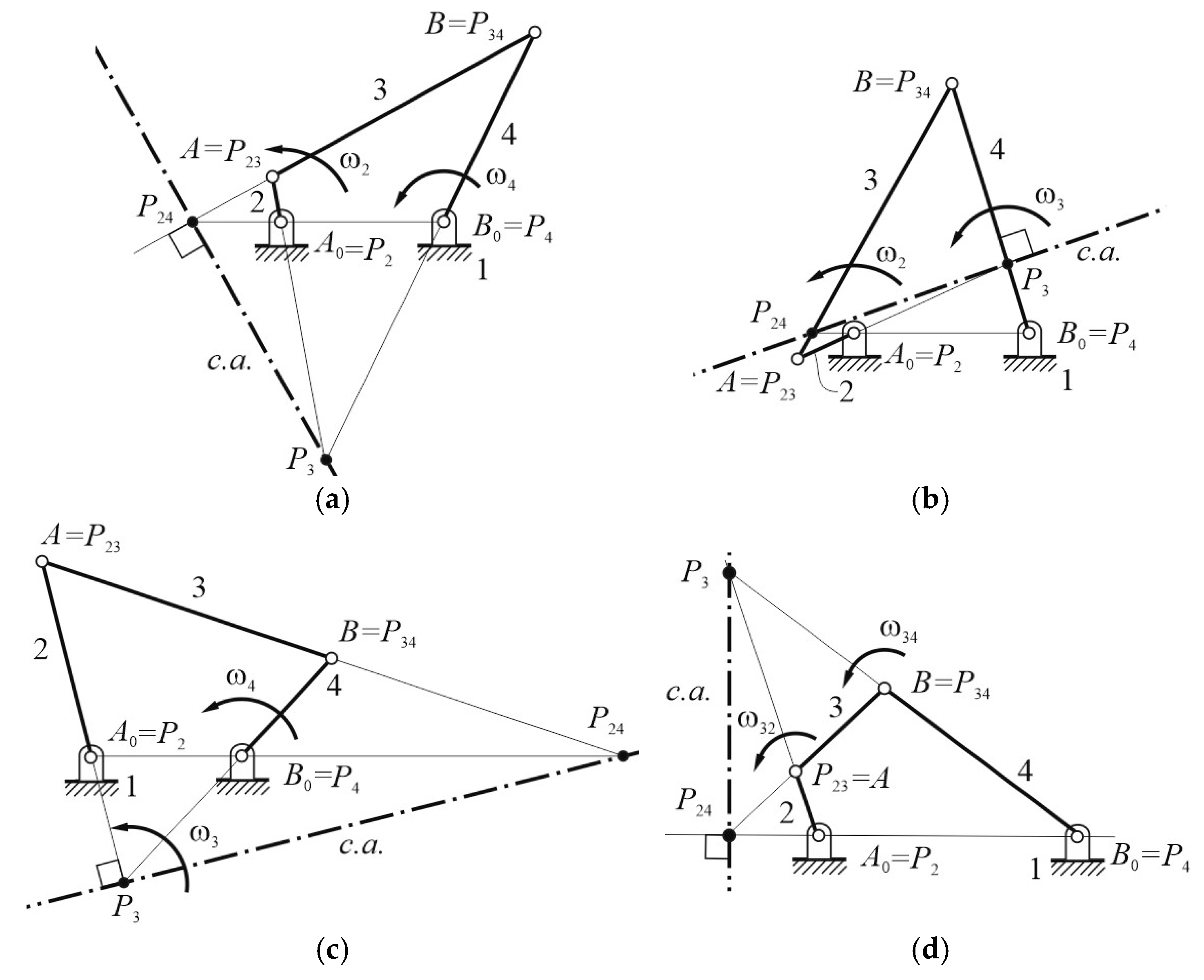
3. Collineation Axis

Referring to Figure 2, Bobillier’s theorem for the four-bar linkage A₀ABB₀ states what follows: the counterclockwise angle ψ₃, which is made by the collineation axis c.a. joining the instant centers (ICs) P₃ and P₂₄ with the rotating link A₀A, is equal to the same oriented angle that is made by rotating link B₀B with the pole tangent t₃.

This theorem is strictly connected to the Aronhold–Kennedy theorem, which allows the determination of all ICs of a mechanism, along with, in particular, the obtaining of P₂ = A₀, P₂₃ = A, P₄ = B₀, and P₃₄ = B by the kinematic properties of the revolute joints. Consequently, P₂₄ and P₃ are, respectively, given by the intersections between of the two straight lines passing through the ICs P₂–P₄ and P₂₃–P₃₄, and likewise through P₂–P₂₃ and P₄–P₃₄.

Thus, the corresponding equations of these straight lines with respect to the fixed frame OXY can be obtained as follows:

$$y-r_{2y}=m_1\left(x-r_{2x}\right)\hspace{1em}\hspace{1em}y-y_{A0}=m_2\left(x-x_{A0}\right)$$

(20)

$$m_1={\displaystyle \frac{r_{2y}-r_{4y}}{r_{2x}-r_{4x}}}\hspace{1em}\hspace{1em}\hspace{1em}\hspace{1em}{m}_2={\displaystyle \frac{y_{A0}-y_{B0}}{x_{A0}-x_{B0}}}$$

(21)

where ($x_{A0}$, $y_{A0}$), ($x_{B0}$, $y_{B0}$), ($r_{2x}$, $r_{2y}$), and ($r_{4x}$, $r_{4y}$) are the Cartesian coordinates of points A₀, B₀, A, and B, respectively. Therefore, by developing Equations (20) and (21), the position vector $r_{P24}$ of P₂₄ in Cartesian form with respect to OXY is given by

$${\mathbf{r}}_{P24}={\displaystyle \frac{1}{m_2-m_1}} \left\{\left(y_{A0}-r_{2y}-m_2{x}_{A0}+m_1{r}_{2x}\right)\mathbf{i}+\left[m_1{y}_{A0}-m_2{r}_{2y}+m_1{m}_2\left(r_{2x}-x_{A0}\right)\right]\mathbf{j}\right\}$$

(22)

Consequently, the collineation axis c.a. can be expressed as follows:

$$\left({\mathbf{r}}_{P3}-{\mathbf{r}}_{P24}\right)\times \left({\mathbf{r}}_Q-{\mathbf{r}}_{P24}\right)=\mathbf{0}$$

(23)

where $r_Q$ is the position vector of point Q, which is a generic point of the c.a.

By developing Equation (23) and simplifying it in Cartesian form, one has

$$y={\displaystyle \frac{r_{P24y}-r_{P3y}}{r_{P24x}-r_{P3x}}}\left(x-r_{P24x}\right)+r_{P24y}$$

(24)

where ($r_{P3x}$, $r_{P3y}$) and ($r_{P24x}$, $r_{P24y}$) are the Cartesian components of $r_{P3}$ and $r_{P24}$.

In a four-bar linkage, Freudenstein’s Theorem 1 states that when the input–output velocity ratio is stationary, the c.a. is perpendicular to the coupler link AB (or r₃). This configuration is shown in Figure 3a, where links 2 and 4 serve as the input and output, respectively. The angular velocity ratio τ₂₄ can be expressed in the form

$${\tau }_{24}={\displaystyle \frac{{\omega }_4}{{\omega }_2}}$$

(25)

where ω₄ is expressed by Equation (9) and ω₂ is the input angular velocity of the mechanism. Two significant scenarios arise from Equation (25).

In particular, when τ₂₄ equals zero, this implies that ω₄ is also zero. In this case, IC P₃ coincides with point B, and point A₀ with P₂₄. Consequently, the c.a. aligns with the coupler link AB.

When τ₂₄ equals 1, this implies that ω₄ is equal to ω₂. Thus, point P₂₄ tends towards infinity because ω₂₄ becomes zero. As a result, the c.a. becomes parallel to both the coupler link AB and the fixed link A₀B₀ (or r₁).

Freudenstein’s Theorem 2 states that at a stationary value of the angular velocity ratio between the coupler and one of the frame-adjacent links, the c.a. is perpendicular to the opposite frame-adjacent link. Figure 3b illustrates a configuration where links 2 and 3 are the input and output links, respectively. The angular velocity ratio τ₂₃ is given by

$${\tau }_{23}={\displaystyle \frac{{\omega }_3}{{\omega }_2}}$$

(26)

where ω₃ is expressed by Equation (8). Figure 3c shows another configuration with links 4 and 3 as the input and output links, respectively. One has the angular velocity ratio τ₄₃

$${\tau }_{43}={\displaystyle \frac{{\omega }_3}{{\omega }_4}}$$

(27)

By considering Equations (26) and (27), significant conditions can be obtained. In particular, when both τ₂₃ and τ₄₃ equal zero, this implies that ω₃ is also zero. In this specific kinematic configuration, point P₃ tends to infinity, and the c.a. becomes parallel to both the input link A₀A and the output link B₀B. When τ₂₃ equals 1, it means that ω₃ is equal to ω₂. In this situation, point P₂₄ coincides with point B, and point A₀ with P₃. Consequently, the c.a. aligns with the fixed link A₀B₀. When τ₄₃ equals 1, it implies that ω₃ is equal to ω₄. In this case, point P₂₄ coincides with point A, and point B₀ with P₃. Similarly to the previous scenario, the c.a. also aligns with the fixed link A₀B₀.

Freudenstein’s Theorem 3 states that at a stationary value of the relative angular velocities between the coupler link and each of the frame-adjacent links, specifically ω₃₂ and ω₃₄, the c.a. is perpendicular to the line of centers A₀B₀. Figure 3d shows such a configuration of a four-bar linkage. The relative angular velocity ratio τ_R can be expressed as follows:

$${\tau }_R={\displaystyle \frac{{\omega }_3-{\omega }_2}{{\omega }_3-{\omega }_4}}={\displaystyle \frac{{\omega }_{32}}{{\omega }_{34}}}$$

(28)

Two significant conditions can be deduced from Equation (28). In particular, when τ_R equals zero, this implies that ω₃ is equal to ω₂. This condition is equivalent to the case of τ₂₃ equals 1, as described in Freudenstein’s Theorem 2, where the c.a. aligns with the fixed link A₀B₀. When τ_R equals 1, this implies that ω₄ is equal to ω₂. This corresponds to the condition of τ₂₄ equals 1 in Freudenstein’s Theorem 1, where the c.a. becomes parallel to both the coupler link AB and the fixed link A₀B₀.

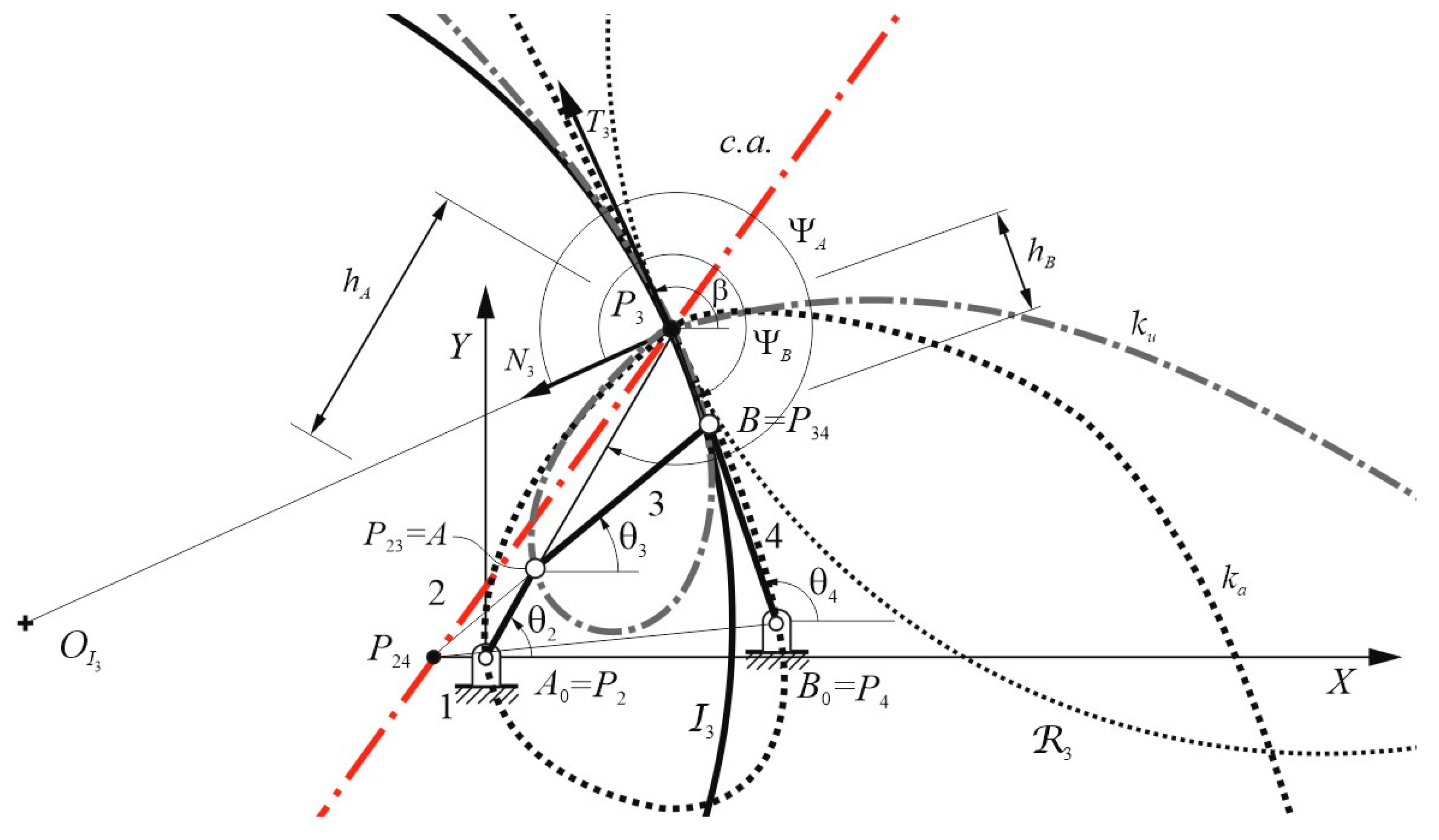
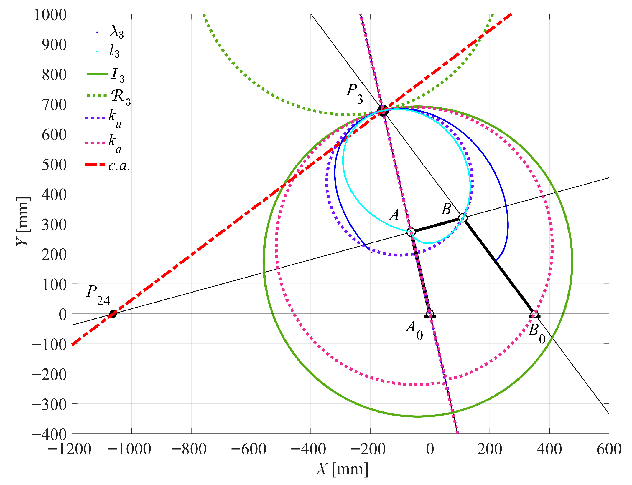
4. Kinematic Analysis: Geometric Loci

Inflection circle I₃ is the geometric locus of the coupler points, which shows an inflection point in their paths and is always tangent to both centrodes at the instantaneous center of rotation P₃. By considering a generic point M of coupler link AB, the equation of inflection circle I₃ can be conveniently obtained by imposing a zero-cross product, as follows:

$${\mathbf{v}}_M\times {\mathbf{a}}_M=\mathbf{0}$$

(29)

where M is a generic coupler point of link 3. In particular, vectors ${\mathbf{v}}_M$ and $a_M$ are obtained by Equations (13) and (17) for B = M and referring to the velocity and acceleration vectors of point A. Thus, substituting ${\mathsf{\omega }}_3$ and ${\mathsf{\alpha }}_3$ of Equations (8) and (10) into Equations (13) and (17), one has ${\mathbf{v}}_M$ and ${\mathbf{a}}_M$ in matrix form:

$${\mathbf{v}}_M=\left[\begin{array}{c}{r}_{2y}\left({\omega }_3-{\omega }_2\right)-{\omega }_{3}y\\ r_{2x}\left({\omega }_2-{\omega }_3\right)+{\omega }_{3}x\\ 0\end{array}\right]$$

(30)

$${\mathbf{a}}_M=\left[\begin{array}{c}{r}_{2x}\left({\omega }_3^2-{\omega }_2^2\right)+r_{2y}\left({\alpha }_3-{\alpha }_2\right)-{\omega }_3^{2}x-{\alpha }_{3}y\\ r_{2x}\left({\alpha }_2-{\alpha }_3\right)+r_{2y}\left({\omega }_3^2-{\omega }_2^2\right)+{\alpha }_{3}x-{\omega }_3^{2}y\\ 0\end{array}\right]$$

(31)

where $r_{2x}$ and $r_{2y}$, along with x and y, are the Cartesian components of ${\mathbf{r}}_A$ and ${\mathbf{r}}_M$, respectively. Therefore, substituting Equations (30) and (31) into Equation (29), and developing it, one has the following algebraic equation of the inflection circle I₃

$$\begin{array}{l}\left[r_{2y}\left({\omega }_3-{\omega }_2\right)-{\omega }_{3}y\right]\cdot \left[r_{2x}\left({\alpha }_2-{\alpha }_3\right)+r_{2y}\left({\omega }_3^2-{\omega }_2^2\right)+{\alpha }_{3}x-{\omega }_3^{2}y\right]-\\ \left[r_{2x}\left({\omega }_2-{\omega }_3\right)+{\omega }_{3}x\right]\cdot \left[r_{2x}\left({\omega }_3^2-{\omega }_2^2\right)+r_{2y}\left({\alpha }_3-{\alpha }_2\right)-{\omega }_3^{2}x-{\alpha }_{3}y\right]=0.\end{array}$$

(32)

Simplifying Equation (32), one can obtain the following expression:

$$x^2+y^2+{𝒜}_{I3}x+{ℬ}_{I3}y+C_{I3}=0$$

(33)

where

$$\begin{gathered} {𝒜}_{I3}={\displaystyle \frac{r_{2x}\left({\omega }_3^2{\omega }_2-2{\omega }_3^3+{\omega }_2^2{\omega }_3\right)+r_{2y}\left({\omega }_3{\alpha }_2-{\omega }_2{\alpha }_3\right)}{{\omega }_3^3}} \\ {ℬ}_{I3}={\displaystyle \frac{r_{2x}\left(-{\omega }_3{\alpha }_2+{\omega }_2{\alpha }_3\right)+r_{2y}\left({\omega }_3^2{\omega }_2-2{\omega }_3^3+{\omega }_2^2{\omega }_3\right)}{{\omega }_3^3}} \\ {C}_{I3}={\displaystyle \frac{\left({\omega }_2-{\omega }_3\right)\left\{r_{2x}\left[r_{2x}\left({\omega }_2^2-{\omega }_3^2\right)+r_{2y}\left({\alpha }_2-{\alpha }_3\right)\right]-r_{2y}\left[r_{2x}\left({\alpha }_2-{\alpha }_3\right)-r_{2y}\left({\omega }_2^2-{\omega }_3^2\right)\right]\right\}}{{\omega }_3^3}} \end{gathered}$$

(34)

The return circle $ℛ$₃ can be obtained by mirroring the inflection circle I₃ with respect to the tangent line t₃ at point P₃, as seen in Figure 2.

As is well known, the coupler motion can be replaced by the pure-rolling of the moving centrode on the fixed one, which are traced by the corresponding IC. In particular, referring to the coupler link AB of the four-bar linkage A₀ABB₀ of Figure 2, the IC P₃ traces the fixed centrode λ₃ on the fixed plane OXY, and likewise the moving centrode l₃ on O₃x₃y₃. Thus, λ₃ is given by Equation (15), while l₃ in O₃x₃y₃, takes the form:

$${\mathbf{r}}_{P3}^{*}=r_3{\displaystyle \frac{\sin \left({\theta }_4-{\theta }_3\right)}{\sin \left({\theta }_4-{\theta }_2\right)}}{\left[\begin{array}{cc}\cos \left({\theta }_2-{\theta }_3\right),& \sin \left({\theta }_2-{\theta }_3\right), 0\end{array}\right]}^{ T}$$

(35)

where symbol T indicates the transpose matrix.

In order to express the moving centrodes l₃ of the coupler link 3 with respect to the fixed frame OXY, the vector function of Equation (35) takes the form:

$$\mathbf{r}=\mathbf{T}{\mathbf{r}}_{P3}^{*}$$

(36)

where T is the following homogeneous transformation matrix by O₃x₃y₃ to OXY as follows:

$$\mathbf{T}=\left[\begin{array}{ccc}\cos {\theta }_3& -\sin {\theta }_3& x_{O3}\\ \sin {\theta }_3& \cos {\theta }_3& y_{O3}\\ 0& 0& 1\end{array}\right]$$

(37)

Particular points on the moving plane have a stationary curvature, i.e., the rate of change in their curvature radius with respect to reference position is zero.

Referring to Figure 4 and to study the trajectories of the coupler points, the canonical reference frame having its origin in P₃, the x-axis along the pole being tangent T₃ to both centrodes l₃ and λ₃, and the y-axis coinciding with the corresponding normal N₃ in P₃ that is oriented toward the center OI₃ of the inflection circle I₃, are conveniently introduced.

The circling-point curve k_u, also known as cubic of stationary curvature, is the locus of all coupler points whose paths have at least four contact points with their osculating circles, thus having a stationary curvature. This geometric locus is represented by a third-order algebraic curve that is named strophoid and denoted as α-curve.

In particular, points A and B of the generic four-bar linkage A₀ABB₀ of Figure 4 have a stationary curvature, since their paths are circles of centers A₀ and B₀, respectively.

The equation of the k_u curve can be expressed in polar form as follows:

$${\displaystyle \frac{1}{h}}={\displaystyle \frac{1}{M \mathrm{s}\mathrm{i}\mathrm{n}\mathsf{\Psi }}}+{\displaystyle \frac{1}{N \mathrm{c}\mathrm{o}\mathrm{s}\mathsf{\Psi }}}$$

(38)

where the coefficients M and N are the instantaneous geometric invariants, h is the oriented segment defining the position of a generic coupler point P, and Ψ is the corresponding clockwise oriented angle with respect to N₃-axis of the P₃T₃N₃ canonical frame.

The coefficients M and N can be determined by substituting the polar coordinates $\left(h_A,{\mathsf{\Psi }}_A\right)$ and $\left(h_B,{\mathsf{\Psi }}_B\right)$ of points A and B of ku in Equation (35), thus obtaining

$${\displaystyle \frac{1}{h_A}}={\displaystyle \frac{1}{M \mathrm{s}\mathrm{i}\mathrm{n}{\mathsf{\Psi }}_A}}+{\displaystyle \frac{1}{N \mathrm{c}\mathrm{o}\mathrm{s}{\mathsf{\Psi }}_A}}$$

(39)

$${\displaystyle \frac{1}{h_B}}={\displaystyle \frac{1}{M \mathrm{s}\mathrm{i}\mathrm{n}{\mathsf{\Psi }}_B}}+{\displaystyle \frac{1}{N \mathrm{c}\mathrm{o}\mathrm{s}{\mathsf{\Psi }}_B}}$$

(40)

which can be solved to achieve M and N in the following form:

$$M={\displaystyle \frac{h_A{h}_B\mathrm{s}\mathrm{i}\mathrm{n}\left({\mathsf{\Psi }}_A-{\mathsf{\Psi }}_B\right)}{\mathrm{s}\mathrm{i}\mathrm{n}{\mathsf{\Psi }}_A\sin {\mathsf{\Psi }}_B\left(h_A\mathrm{c}\mathrm{o}\mathrm{s}{\mathsf{\Psi }}_B-h_B\mathrm{c}\mathrm{o}\mathrm{s}{\mathsf{\Psi }}_A\right)}}$$

(41)

$$N=-{\displaystyle \frac{h_A{h}_B\mathrm{s}\mathrm{i}\mathrm{n}\left({\mathsf{\Psi }}_A-{\mathsf{\Psi }}_B\right)}{\mathrm{c}\mathrm{o}\mathrm{s}{\mathsf{\Psi }}_A\cos {\mathsf{\Psi }}_B\left(h_A\mathrm{s}\mathrm{i}\mathrm{n}{\mathsf{\Psi }}_B-h_B\mathrm{s}\mathrm{i}\mathrm{n}{\mathsf{\Psi }}_A\right)}}$$

(42)

The equation of the k_u curve can also be expressed in Cartesian form as follows:

$$\left({\nu }^2+{\mu }^2\right)\left({\displaystyle \frac{\nu }{M}}+{\displaystyle \frac{\mu }{N}}\right)-\nu \mu =0$$

(43)

where ν and μ are given by

$$\nu ={\displaystyle \frac{y-r_{P3y}+\left(x-r_{P3x}\right)\tan \beta }{\tan \beta \sin \beta +\cos \beta }}$$

(44)

$$\mu ={\displaystyle \frac{x-r_{P3x}+\nu \sin \beta }{\cos \beta }}$$

(45)

where β is the counterclockwise-oriented angle made by the abscissa T3-axis of the canonical frame, with respect to the x-axis of OXY, as shown in Figure 4.

The locus of the centers of curvature of all points lying on k_u is still a circular cubic, also known as centering-point curve k_a, which can be expressed by

$$\left({\mathsf{\Gamma }}^2+{\mathsf{\Pi }}^2\right)\left({\displaystyle \frac{\mathsf{\Gamma }}{\overline{M}}}+{\displaystyle \frac{\mathsf{\Pi }}{\overline{N}}}\right)-\mathsf{\Gamma } \mathsf{\Pi }=0$$

(46)

where

$$\mathsf{\Gamma }={\displaystyle \frac{y-r_{P3y}+\left(x-r_{P3x}\right)\tan \beta }{-\left(\tan \beta \sin \beta +\cos \beta \right)}}$$

(47)

$$\mathsf{\Pi }={\displaystyle \frac{x-r_{P3x}-\mathsf{\Gamma }\sin \beta }{-\cos \beta }}$$

(48)

$${\displaystyle \frac{1}{\overline{N}}}={\displaystyle \frac{1}{\delta }}+{\displaystyle \frac{1}{N}}\hspace{1em}\hspace{1em}\hspace{1em}\hspace{1em}\overline{N}={\displaystyle \frac{\delta N}{\delta -N}}$$

(49)

$${\displaystyle \frac{1}{\overline{M}}}=-{\displaystyle \frac{1}{M}}\hspace{1em}\hspace{1em}\hspace{1em}\hspace{1em}\overline{M}=-M$$

(50)

where δ is the diameter of the inflection circle I₃.

In general, both the k_u and k_a curves are strophoids (or α-curves), as observed in Figure 4. The intersection of the k_u curve and the infection circle I₃ defines Ball’s point, which is a point in the moving plane that describes a straight line with a third-order approximation or more. All points on the k_u curve have a stationary curvature and those lying on the inflection circle show an inflection point of their paths. Thus, Ball’s point is the intersecting point of the cubic of stationary curvature k_u and the inflection circle I₃.

The IC P₃ gives information about the velocities of all coupler points, and the inflection circle I₃ provides information about those with zero acceleration (or infinite radius of curvature). Instead, the k_u curve refers to the third-order properties of motion, particularly when the radius of curvature of a point’s path is momentarily constant. It is often used in mechanism synthesis, particularly for path generation, where a coupler point is required to follow a specific path, with certain curvature properties.

The degeneration of the k_u curve and its corresponding k_a curve is a specialized concept in kinematics that describes when this higher-order curve, which determines points of stationary curvature, simplifies into more basic geometric forms, like a circle and a line. This simplification is not random; it is a consequence of specific kinematic configurations of the mechanism and often corresponds to points with particularly desirable or unique path properties, making it relevant for mechanism synthesis and analysis.

In general, the k_u and k_a curves can degenerate into the following: a circle and a straight line or into a ϕ-curve; multiple lines; in some cases, it might even degenerate into three lines, which might include the line at infinity; and an equilateral hyperbola together with the straight line at infinity. This paper highlights how the angular velocity ratios (τ₂₄, τ₂₃, τ₄₃, and τ_R) are central parameters for understanding the kinematic behavior of a mechanism. By carefully observing these ratios and their derivatives, one can discover specific configurations, including singular or maximum/minimum positions, that lead to the simplification of complex k_u and k_a curves, which are extremely useful for mechanism design and analysis. In a four-bar linkage, specific configurations lead to extreme velocity ratios and characteristic behaviors of the inflection circle’s diameter and the c.a.

When a mechanism reaches configurations with extreme velocity ratios (τ₂₄, τ₂₃, τ₄₃ and τ_R), the inflection circle’s diameter remains stationary. This occurs when each of the links (r₃, r₄, r₂, and r₁) forms a 90° angle with the c.a., as detailed in Section 3.

The angular velocity ratios, τ₂₄, τ₂₃, τ₄₃, and τ_R, can be plotted against the corresponding input angle θ₂ for the four-bar linkage, as shown in Figure 5. This plot helps to identify four values for each ratio: their maximum and minimum values, and when they equal 0 and 1. When τ₂₄ is at its minimum or maximum values, as seen in Figure 6a, the c.a. becomes orthogonal to the coupler link AB. In this state, the k_u curve degenerates into a ϕ-curve, which is a circle passing through the points A, B, and P₃. It also forms a straight line that coincides with the tangent t₃ to the inflection circle I₃ at the IC P₃. In the case where τ₂₃ is at its minimum or maximum values, as seen in Figure 6b, the c.a. becomes orthogonal to the output link B₀B. In this configuration, both the k_u and k_a curves degenerate into ϕ-curves. This results in the following: a circle passing through points A and P₃; another circle passing through points B₀ and P₃; a straight line that passes through points A₀ and A, coinciding with the tangent t₃ to the inflection circle I₃ at point P₃. A special case can be obtained when τ₂₄ is at its minimum or maximum values, as seen in Figure 6c: The c.a. becomes parallel to both the input link A₀A and the output link B₀B, and it also becomes perpendicular to the coupler link AB. In this specific configuration, point P₃ tends to infinity. This causes the k_a curve to degenerate into an equilateral hyperbola that passes through the points A₀, A, and P₃ (at infinity), including the line at infinity. Simultaneously, the k_u curve degenerates into two straight lines: one passing through points A and B, and the other parallel to P₃, along with a line at infinity.

5. Numerical Examples

To validate the general algorithm for the synthesis of four-bar mechanisms, it was implemented in Matlab (2018b) and tested through several significant examples. As shown in Figure 7, a flowchart of the proposed algorithm is provided to enhance clarity and reproducibility, illustrating the sequence of calculations and referencing the relevant equations.

Table 1. Numerical examples.

Case of Study	r1 (A0B0) [mm]	r2 (A0A) [mm]	r3 (AB) [mm]	r4 (B0B) [mm]	Figures
Case 1: Crank-rocker	250	80	200	190	Figure 8, Figure 9, Figure 10, Figure 11 and Figure 12
Case 2: Crank-rocker	400	100	400	300	Figure 13
Case 3: Crank-rocker	400	100	400	400	Figure 14
Case 4: Double-crank	100	220	185	180	Figure 15, Figure 16, Figure 17 and Figure 18
Case 5: Double-rocker	350	280	180	400	Figure 19, Figure 20, Figure 21 and Figure 22
Case 6: Triple-rocker	100	110	200	150	Figure 23, Figure 24, Figure 25 and Figure 26

details the dimensions of these mechanisms, all with an angular velocity ω₂ of 1 r/s. The examples include Cases 1–3 as crank-rocker mechanisms, Case 4 as a double-crank, Case 5 as a double-rocker, and Case 6 as a triple-rocker.

Case 1: A crank-rocker mechanism is analyzed in detail, with its results shown in Figure 8, Figure 9, Figure 10, Figure 11 and Figure 12 and

Table 2. Case 1 (Crank-rocker): Special cases of k_u and k_a according to Freudenstein’s Theorem.

	Values	θ2 [°]	ku	ka	Conditions		Figure
τ24MIN	−0.5236	343.7667	ϕ-curve	α-curve	c.a. ⊥ AB		Figure 9b
τ24MAX	0.4258	119.8000	ϕ-curve	α-curve	c.a. ⊥ AB		Figure 9a
τ24	0	41.5333	α-curve	ϕ-curve	c.a. in-line AB	P3 ≡ B, P24 ≡ A0	Figure 9c
τ24	0	227.1667	α-curve	ϕ-curve	c.a. in-line AB	P3 ≡ B, P24 ≡ A0	Figure 9d
τ23MIN	−0.5022	12.7333	ϕ-curve	ϕ-curve	c.a. ⊥ B0B		Figure 10a
τ23MAX	0.4059	237.4333	ϕ-curve	ϕ-curve	c.a. ⊥ B0B		Figure 10b
τ23	0	128.9667	) ( - curve	) ( - curve	c.a. || A0A || B0B	P3→∞	Figure 10c
τ23	0	314.9667	) ( - curve	) ( - curve	c.a. || A0A || B0B	P3→∞	Figure 10d
τ43	1	0	ϕ-curve	α-curve	c.a. in-line A0B0	P3 ≡ B0, P24 ≡ A	Figure 11a
τ43	1	180.0000	ϕ-curve	α-curve	c.a. in-line A0B0	P3 ≡ B0, P24 ≡ A	Figure 11b
τRMINREL	2.5150	102.3667	α-curve	ϕ-curve	c.a. ⊥ A0B0		Figure 12a
τRMAXREL	−1.2017	257.1000	α-curve	ϕ-curve	c.a. ⊥ A0B0		Figure 12b

. Referring to Figure 8, the diagrams of the velocity ratios τ₂₄, τ₂₃, τ₄₃, and τ_R are analyzed as functions of the input angle θ₂ and thus, they are represented in Figure 8a, b, c, and d, respectively. Particular attention is given to the maximum and minimum values of these ratios, as well as where they equal 0 or 1. A key aspect of the study is the correlation between these velocity ratios, the c.a., and the degeneration of k_u and k_a curves into special curves. This detailed examination of Case 1 offers valuable insights into the kinematic behavior of crank-rocker mechanisms, specifically regarding the transmission angle, other velocity ratios, and the geometric properties of their associated curves at critical configurations. In addition, each figure illustrating a case study includes a legend that clearly distinguishes the following geometric loci: the fixed centrode λ₃ (blue, dot line), the moving centrode l₃ (cyan, dot line), the inflection circle I₃ (green, solid line), the return circle $ℛ$₃ (green, dotted line), the k_u curve (magenta dark, dotted line), the k_a curve (magenta light, dotted line), and the collineation axis c.a. shown in red with a dash-dotted line. For velocity ratio τ₂₄, the specific results of Case 1 are as follows:

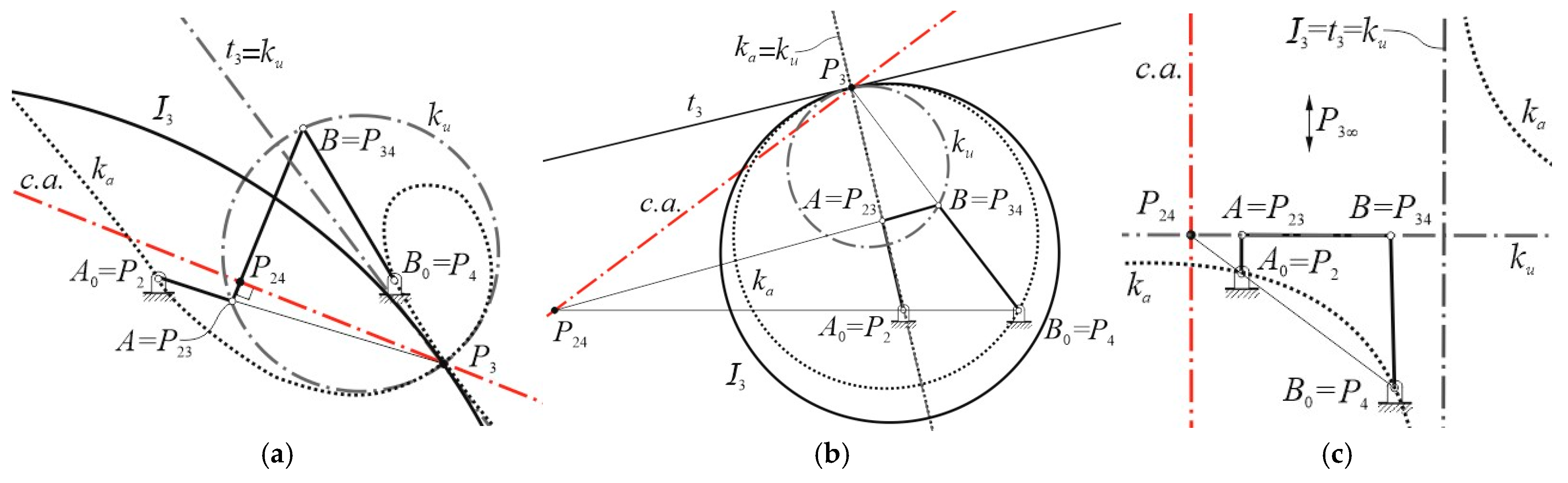
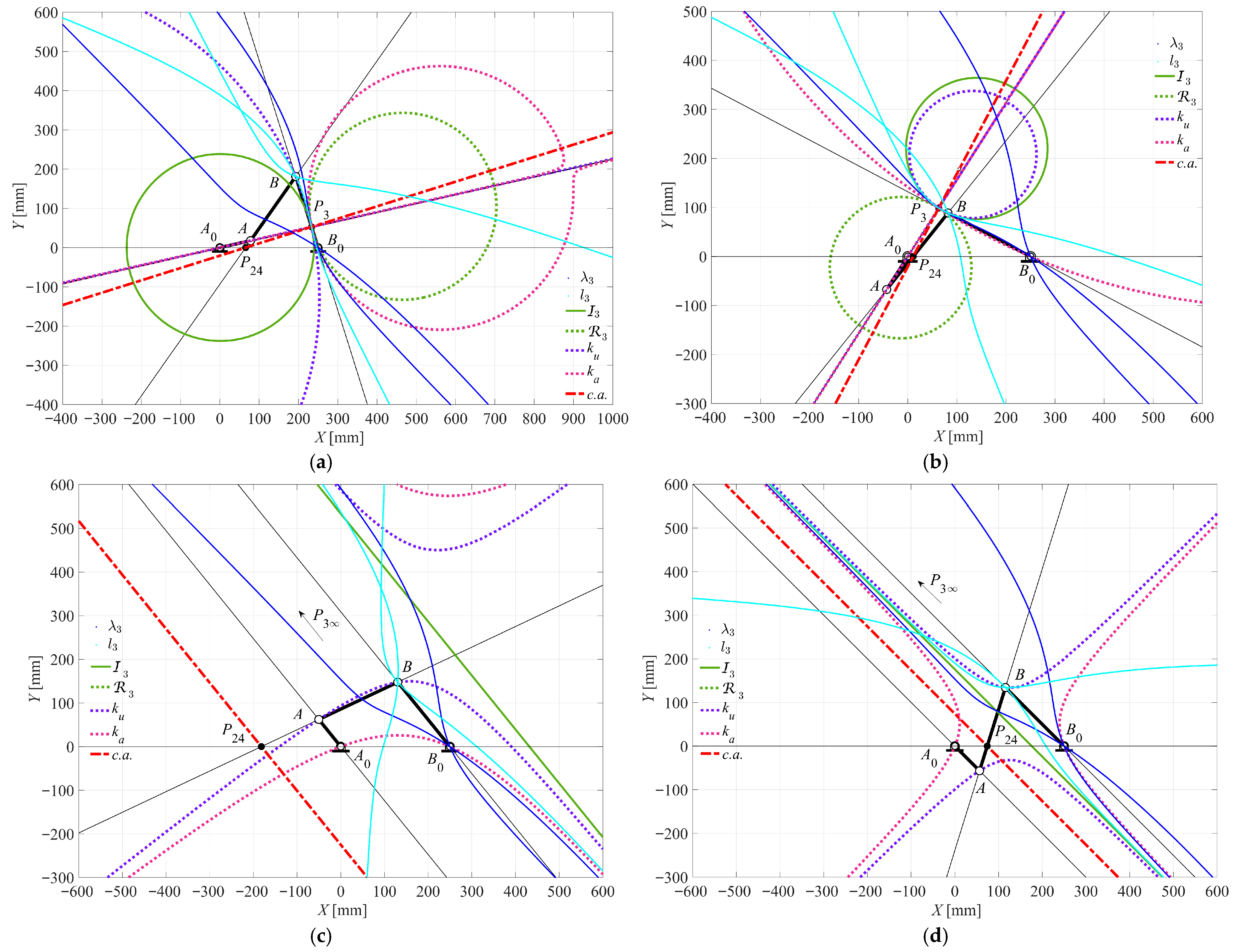
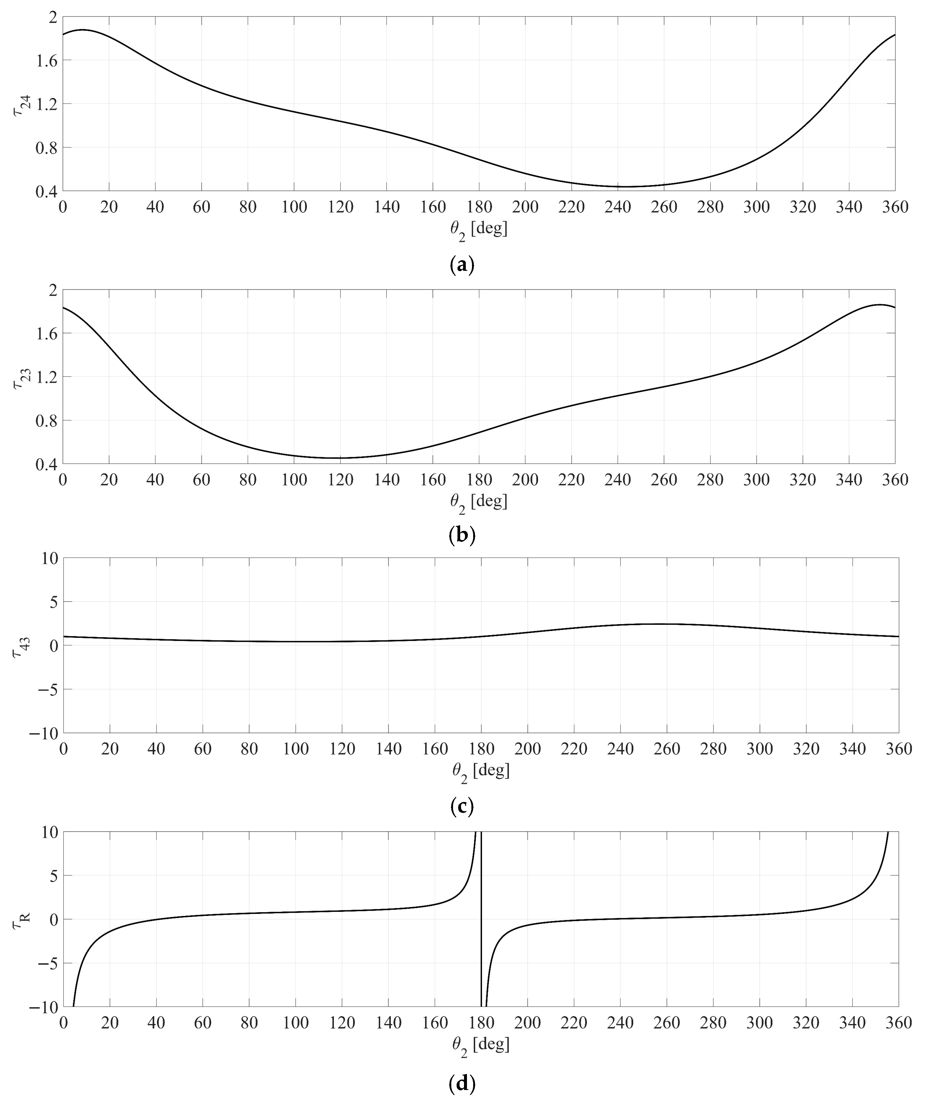
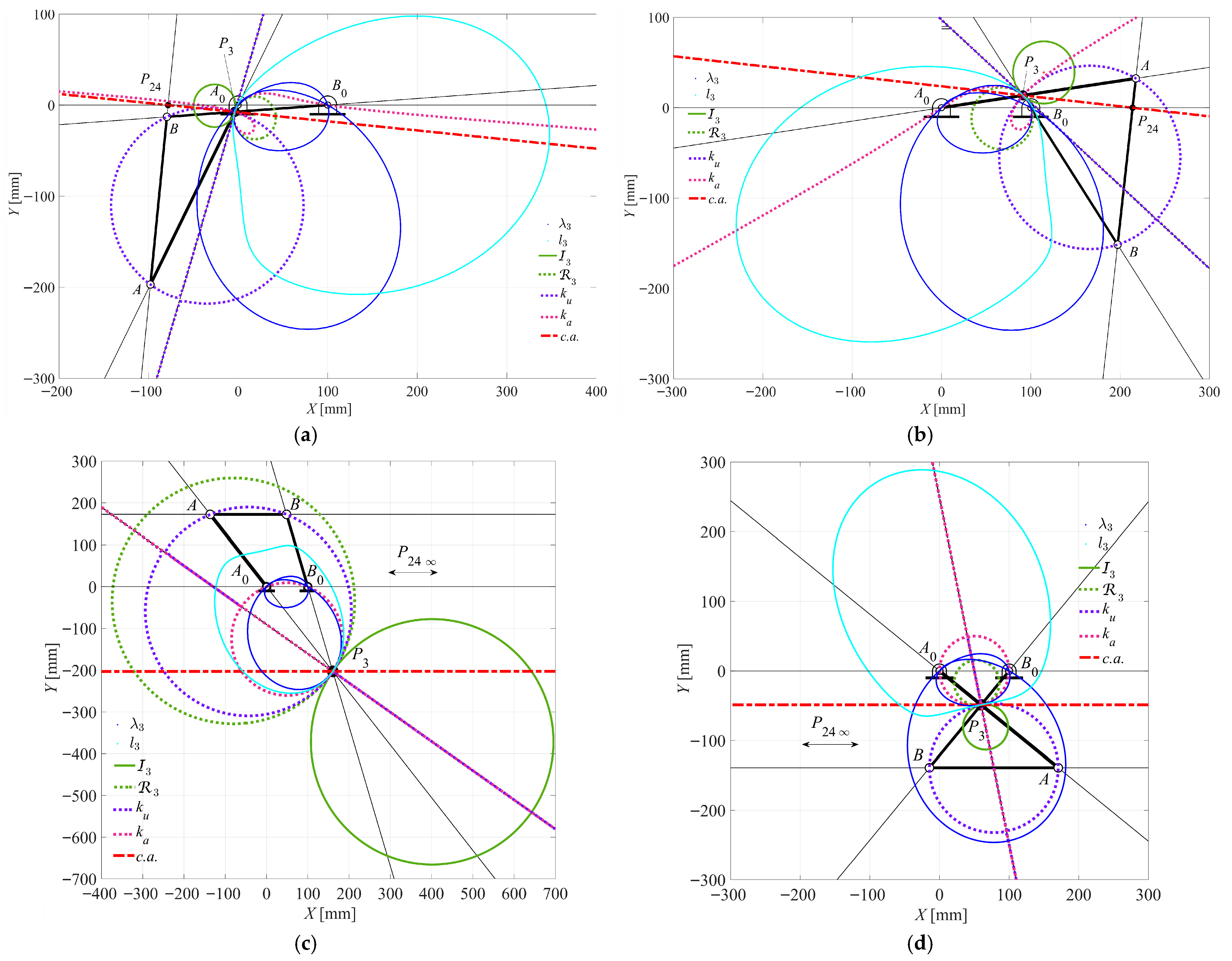
• The minimum τ_24MIN = −0.5236 occurs at θ₂ = 343.7667°. At this point, the c.a. is orthogonal to the coupler link AB. The k_u curve degenerates into a ϕ-curve: a circle through points A, B, and P₃, and a line coinciding with the tangent t₃ to the I₃ at P₃, as seen in Figure 9a.
• The maximum τ_24MAX = 0.4258 occurs at θ₂ = 119.8000°. Similarly to the minimum, the c.a. is orthogonal to the coupler link AB, and the k_u curve degenerates into a ϕ-curve, as reported in Figure 9b.
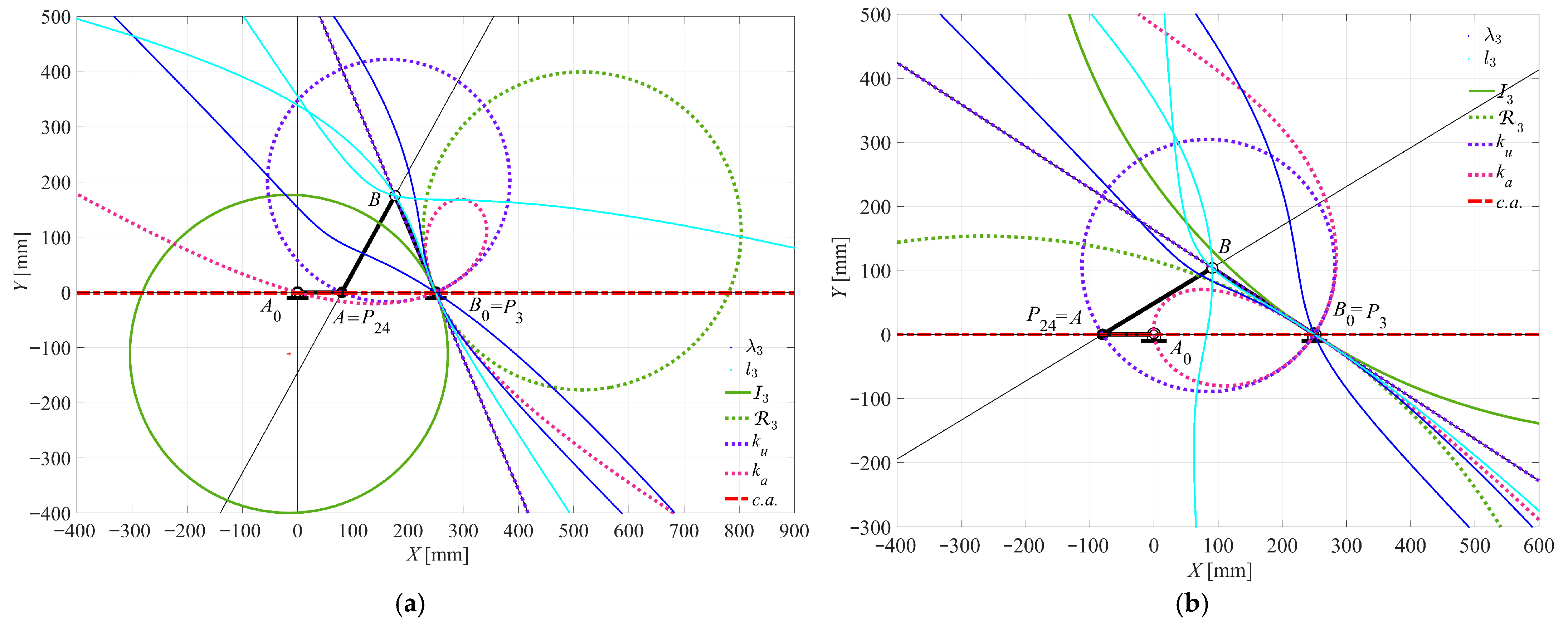
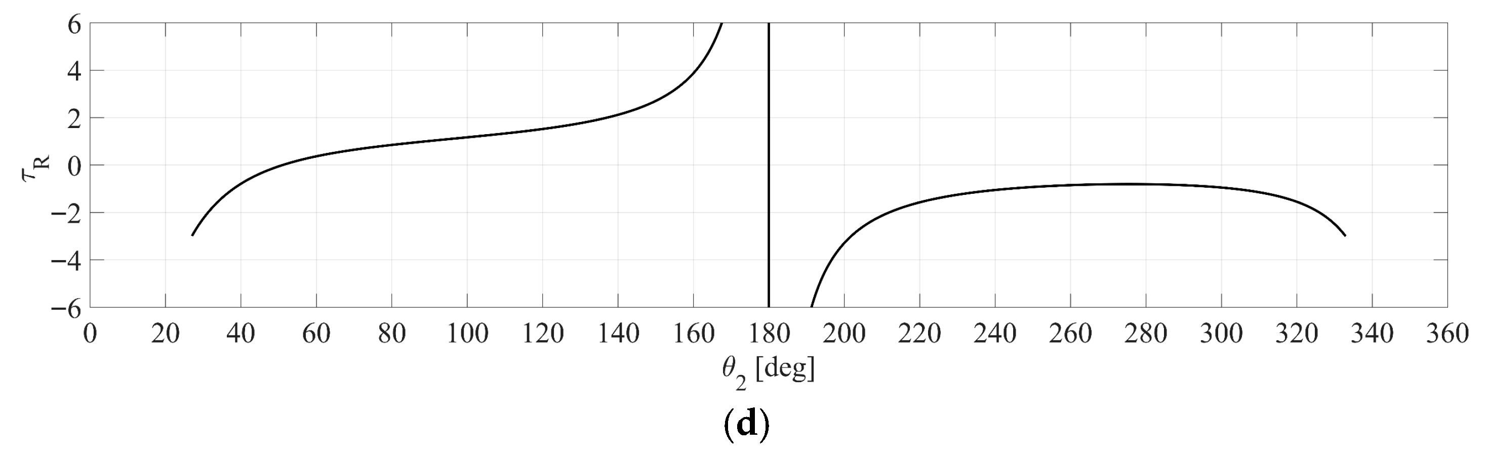
• The τ₂₄ becomes zero at input angles θ₂ = 41.5333° and θ₂ = 227.1667°. In these cases, where the mechanism is in a dead-point configuration, the c.a. is aligned with the coupler link AB. The k_a curve degenerates into a ϕ-curve: a circle passing through P₃ (coinciding with B) and A₀ (coinciding with P₂₄), along with a straight line coincident with the tangent t₃ to the I₃ at P₃, as shown in Figure 9c,d.

For velocity ratio τ₂₃, the specific results of Case 1 are as follows:

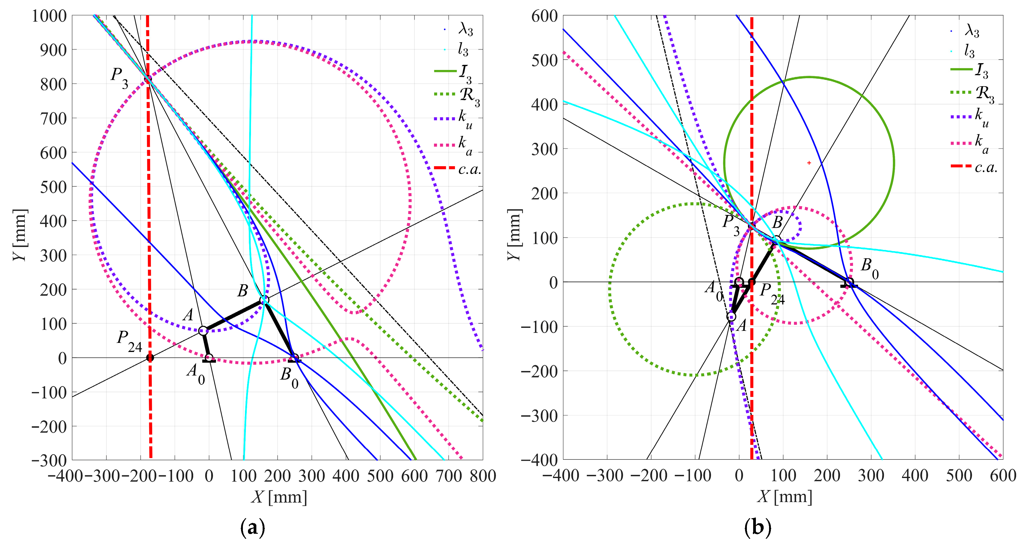
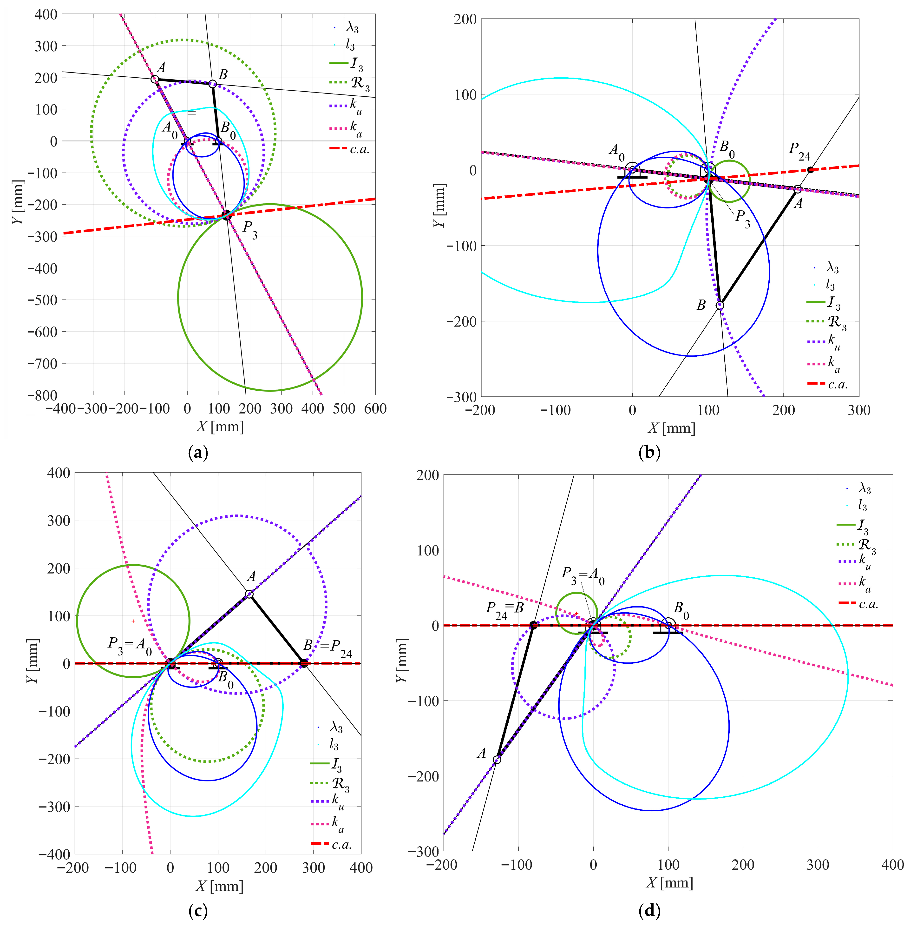
• The minimum τ_23MIN = −0.5022 and the maximum τ_23MAX = 0.4059 occur at θ₂ = 12.7333° and θ₂ = 237.4333°, respectively. The c.a. becomes orthogonal to the coupler link B₀B. Specifically, these ϕ-curves are composed of the following: a circle passing through points P₃ and B₀; another circle passing through points B and P₃; a straight line, which is orthogonal to the tangent t₃ to the I₃ at P₃, passing through points A₀ and A, respectively, as shown in Figure 10a,b.
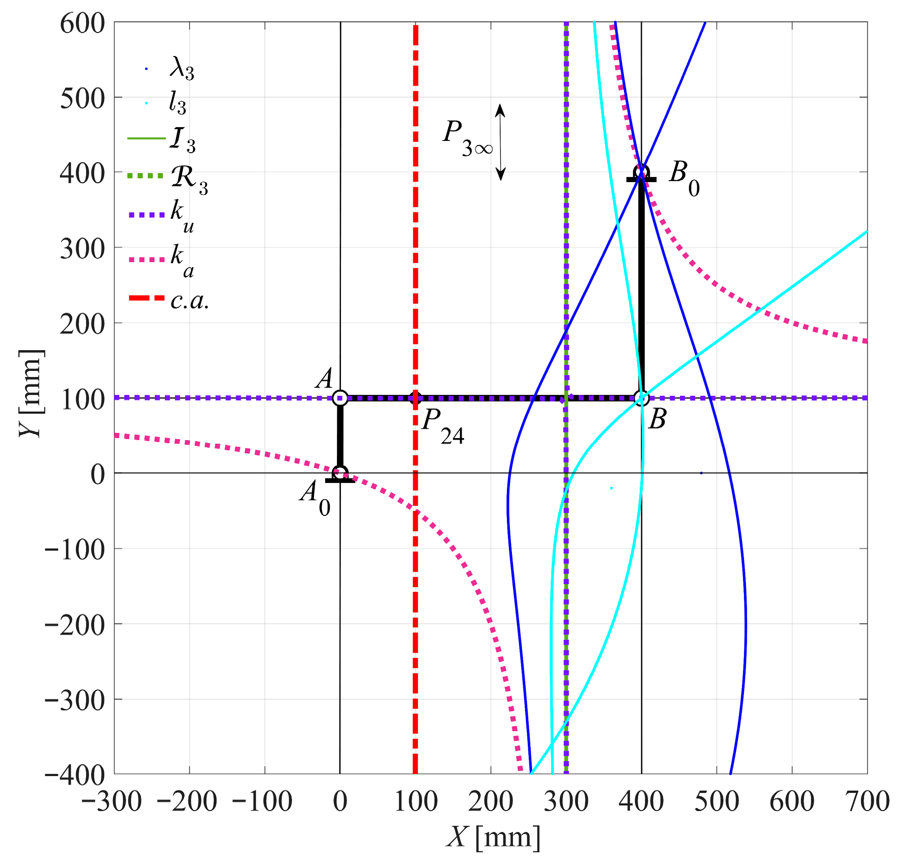
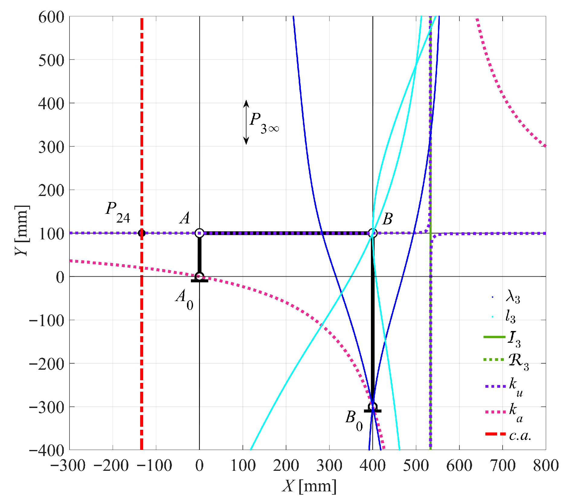
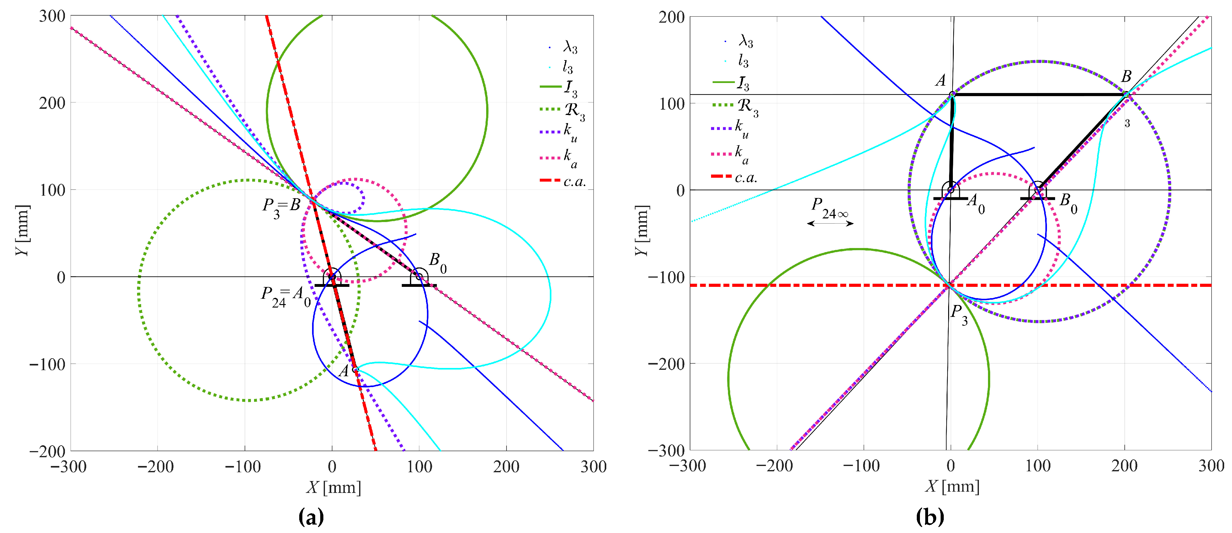
• The τ₂₃ equals 0 occurs at θ₂ = 128.9667° and θ₂ = 314.9667°. The c.a. becomes parallel to both the input link A₀A and the output link B₀B, with P₃ tending to infinity. Under this condition, both the k_a and k_u curves degenerate into equilateral hyperbola (or ) ( - curves). In particular, the k_a curve passes through points A₀, B₀, and P₃ (at infinity), while the k_u curve passes through points A, B, and P₃. Additionally, each branch of these curves is tangent to the I₃, as shown in Figure 10c,d.

For velocity ratio τ₄₃, the specific results of Case 1 are as follows:

• The τ₄₃ equals 1 at θ₂ = 0° and θ₂ = 180°. The c.a. aligns with the fixed link A₀B₀. P₂₄ coincides with point A, and P₃ coincides with point B₀. The k_u curve degenerates into a ϕ-curve (a circle through P₃ and A₀, and a line coincident to t₃ to the I₃ at point P₃, while also passing through A), as shown in Figure 11a,b.

For velocity ratio τ_R, the specific results of Case 1 are as follows:

• The minimum τ_RMINREL = 2.5150 and maximum τ_RMAXREL = −1.2017 relative values occur at θ₂ = 102.3667° and θ₂ = 257.1000°, respectively. The c.a. becomes orthogonal to the fixed link A₀B₀. The k_a curve degenerates into a ϕ-curve (a circle passing through points P₃, A₀, and B₀, as well as a straight line (coincident to the tangent t₃ to I₃ at point P₃), as shown in Figure 12a,b.

Cases 2 and 3, which represent the asymptotic configurations of a crank-rocker mechanism in which links 2, 3, and 4 are mutually orthogonal, are presented in Figure 13 and Figure 14.

When τ₂₄ reaches its minimum τ_24MIN and maximum τ_24MAX values at θ₂ = 90.0000°, the c.a. becomes parallel to both the input link A₀A and the output link B₀B. Simultaneously, it becomes perpendicular to the coupler link AB. In this specific configuration, point P₃ tends to infinity, causing both the k_u and k_a curves to degenerate. Specifically, k_a degenerates into an equilateral hyperbola that passes through points A₀, B₀, and P₃ (at infinity), as well as a line at infinity. Meanwhile, k_u degenerates into two straight lines: the first passes through points A and B, the second is parallel to P₃, and the third is a line at infinity.

Case 4: A double-crank mechanism is analyzed in detail, with its results presented in Figure 15, Figure 16, Figure 17 and Figure 18 and

Table 3. Case 4 (Double-crank): Special cases of k_u and k_a according to Freudenstein’s Theorem.

	Values	θ2 [°]	ku	ka	Conditions		Figure
τ24MIN	0.4390	243.5667	ϕ-curve	α-curve	c.a. ⊥ AB		Figure 16a
τ24MAX	1.8771	8.4667	ϕ-curve	α-curve	c.a. ⊥ AB		Figure 16b
τ24	1	128.3667	ϕ-curve	ϕ-curve	c.a. || A0B0 || AB	P24→∞	Figure 16c
τ24	1	320.8333	ϕ-curve	ϕ-curve	c.a. || A0B0 || AB	P24→∞	Figure 16d
τ23MIN	0.4528	118.1667	ϕ-curve	ϕ-curve	c.a. ⊥ B0B		Figure 17a
τ23MAX	1.8600	353.3333	ϕ-curve	ϕ-curve	c.a. ⊥ B0B		Figure 17b
τ23	1	41.2667	ϕ-curve	α-curve	c.a. in-line A0B0	P3 ≡ A0, P24 ≡ B	Figure 17c
τ23	1	234.2333	ϕ-curve	α-curve	c.a. in-line A0B0	P3 ≡ A0, P24 ≡ B	Figure 17d
τ43MIN	0.4207	104.1000	ϕ-curve	ϕ-curve	c.a. ⊥ A0A		Figure 18a
τ43MAX	2.4292	256.7333	ϕ-curve	ϕ-curve	c.a. ⊥ A0A		Figure 18b
τ43	1	0	ϕ-curve	α-curve	c.a. in-line A0B0	P3 ≡ B0, P24 ≡ A	Figure 18c
τ43	1	180.0000	ϕ-curve	α-curve	c.a. in-line A0B0	P3 ≡ B0, P24 ≡ A	Figure 18d

. The analysis focuses on the behavior of various velocity ratios (τ₂₄, τ₂₃, τ₄₃, and τ_R) as functions of the input angle θ₂, as shown in Figure 15. Specific attention is given to the maximum and minimum values of these ratios, as well as where they equal 0 or 1, as seen in Figure 15. For velocity ratio τ₂₄, the specific results of Case 4 are as follows:

• The minimum τ_24MIN = 0.4390 and the maximum τ_24MAX = 1.8771 at θ₂ = 243.5667° and θ₂ = 8.4667°, respectively. At these points, the c.a. is orthogonal to the coupler link AB. These configurations shown in Figure 16a,b, yielding the same results as those presented in Figure 9a,b.
• The τ₂₄ becomes 1 at input angles θ₂ = 128.3667° and θ₂ = 320.8333°. The c.a. becomes parallel to both the coupler link AB and fixed link A₀B₀. Under this condition, both the k_a and k_u curves degenerate into ϕ-curves, which are composed of the following: a circle passing through points P₃, A₀, and B₀; another circle passing through points A, B, and P₃; a straight line that is orthogonal to the tangent t₃ to the I₃ at point P₃, as illustrated in Figure 16c,d.

For velocity ratio τ₂₃, the specific results of Case 4 are as follows:

• The minimum τ_23MIN = 0.4528 and the maximum τ_23MAX = 1.8600 at θ₂ = 118.1667° and θ₂ = 353.3333°, respectively. At these points, the c.a. is orthogonal to the output link B₀B. These configurations shown in Figure 17a,b, yielding the same results as those presented in Figure 10a,b.
• The τ₂₃ equals 1 occurs at θ₂ = 41.2667° and θ₂ = 234.2333°. In these cases, where the mechanism is in a dead-point configuration, the c.a. is in-line with the coupler link AB. The k_u curve degenerates into a ϕ-curve, which is a circle passing through points P₃ (coinciding with A₀) and B (coinciding with P₂₄). Additionally, there is a straight line that is coincident to the tangent t₃ to the I₃ at point P₃, as shown in Figure 17c,d.

For the velocity ratio τ₄₃, the specific results of Case 4 are as follows:

• The minimum τ_43MIN = 0.4207 and the maximum τ_43MAX = 2.4292 at θ₂ = 104.1000° and θ₂ = 256.7333°, respectively. At these points, where the mechanism is in a dead-point configuration, the c.a. becomes orthogonal to the fixed link A₀A. Both the k_a and k_u curves degenerates into a ϕ-curve, which is specifically defined by the following: a circle that passes through points P₃ and A₀; another circle that passes through points P₃ and A; a straight line that passes through points P₃ and B; a straight line that passes through points and P₃ and B₀. The latter two lines are also coincident to the tangent t₃ to the circle I₃ at point P₃, as shown in Figure 18a,b.
• The τ₄₃ equals 1 at θ₂ = 0° and θ₂ = 180°. The c.a. aligns with the fixed link A₀B₀, and these configurations shown in Figure 18c,d yield the same results as those shown in Figure 11a,b.

Case 5: A double-rocker mechanism is analyzed in detail, with its results presented in Figure 19, Figure 20, Figure 21 and Figure 22 and

Table 4. Case 5 (Double-rocker): Special cases of k_u and k_a according to Freudenstein’s Theorem.

	Values	θ2 [°]	ku	ka	Conditions		Figure
τ24	0	57.2667	α-curve	ϕ-curve	c.a. in-line AB	P3 ≡ B, P24 ≡ A0	Figure 20a
τ24	1	123.6000	ϕ-curve	ϕ-curve	c.a. || A0B0 || AB	P24→∞	Figure 20b
τ23MAX	−0.6733	103.1000	ϕ-curve	ϕ-curve	c.a. ⊥ B0B		Figure 21
τ43MAXREL	−0.8487	112.4333	ϕ-curve	ϕ-curve	c.a. ⊥ A0A		Figure 22

. The analysis focuses on the behavior of various velocity ratios (τ₂₄, τ₂₃, τ₄₃, and τ_R) as functions of the input angle θ₂. Figure 19 highlights the minimum and maximum angular velocity ratios for each velocity ratio, their corresponding θ₂ values, and the specific positions of the c.a. relative to the mechanism’s links.

As shown in Figure 20a, when τ₂₄ equals 0 at θ₂ = 57.2667°, the mechanism is in a dead-point configuration. In this case, the c.a. is aligned with the coupler link AB, consistent with the results presented in Figure 9c. Conversely, τ₂₄ equals 1 at θ₂ = 123.6000°, the c.a. is parallel to both coupler link AB and fixed link A₀B₀, as depicted in Figure 20b. This configuration matches the results shown in Figure 16c,d. Similarly, as illustrated in Figure 21, when τ_23MAX = −0.6733 at θ₂ = 103.1000°, the c.a. is perpendicular to the output link B₀B. This configuration aligns with the results shown in Figure 10b and Figure 17b.

Referring to Figure 22, when τ_43MAXREL = −0.8487 at θ₂ = 112.4333°, the c.a. is perpendicular the input link A₀A. This configuration is consistent with the result shown in Figure 18b.

Case 6: A triple-rocker mechanism is analyzed in detail, with its results presented in Figure 23, Figure 24, Figure 25 and Figure 26 and

Table 5. Case 6 (Triple-rocker): Special cases of k_u and k_a according to Freudenstein’s Theorem.

	Values	θ2 [°]	ku	ka	Conditions		Figure
τ24	0	284.1333	α-curve	ϕ-curve	c.a. in-line A0A	P3 ≡ B, P24 ≡ A0,	Figure 24a
τ24	1	88.9667	ϕ-curve	ϕ-curve	c.a. || A0B0 || AB	P24→∞	Figure 24b
τ23	0	316.3000	) ( - curve	) ( - curve	c.a. || A0A || B0B	P3→∞	Figure 25a
τ23	1	51.0000	ϕ-curve	α-curve	c.a. in-line A0B0	P3 ≡ A0, P24 ≡ B	Figure 25b
τ43	1	180.0000	ϕ-curve	α-curve	c.a. in-line A0B0	P3 ≡ B0, P24 ≡ A	Figure 26

. The analysis focuses on the behavior of various velocity ratios (τ₂₄, τ₂₃, τ₄₃, and τ_R) as functions of the input angle θ₂, as seen in Figure 23. Similar patterns are observed in Figure 24a when τ₂₄ equals 0 at θ₂ = 284.1333°. This dead-point configuration aligns with the results previously presented in Figure 9b,d and Figure 20a.

When τ₂₄ equals 1 at θ₂ = 88.9667°, the asymptotic configuration, shown in Figure 24b, where links 2 and 3 are mutually orthogonal, aligns with the results shown in Figure 16c,d and Figure 20b. Furthermore, as illustrated in Figure 25a, when τ₂₃ equals 0 at θ₂ = 316.3000°, this configuration aligns with the results presented in Figure 10c,d. When τ₂₃ equals 1 at θ₂ = 51.0000°, as shown in Figure 25b, this dead-point configuration aligns with the results presented in Figure 17c,d. Lastly, as shown in Figure 26, when τ₄₃ equals 1 at θ₂ = 180.0000°, this dead-point configuration is consistent with the results shown in Figure 11a,b and Figure 18c,d.

6. Conclusions

A general algorithm to determine the coupler link geometric loci, such as centrodes, inflection and return circles, as well as circling-point and centering-point curves, has been formulated as based on Grashof’s law and Freudenstein’s theorems. The main novelty consists of four diagrams of the angular–velocity ratios versus the mechanism driving angle, since these diagrams allows the identification of all mechanism configurations, with different geometric loci degenerate forms such as straight lines, including the line at infinity, ϕ-curves, and/or equilateral hyperbolas. The proposed algorithm has been implemented in Matlab and validated by means of several significant examples. Asymptotic and dead-point configurations are some of these particular cases, which could be useful for synthesis purposes, as well as for designing six-bar dwell mechanisms or straight-line path generators

References

- Freudenstein, F. On the Maximum and Minimum Velocities and the Accelerations in Four-Link Mechanisms. Trans. Am. Soc. Mech. Eng. 1956, 78, 779–785. [Google Scholar] [CrossRef]
- Wu, L.-I.; Wu, S.-H. A note on Freudenstein’s theorem. Mech. Mach. Theory 1998, 33, 139–149. [Google Scholar] [CrossRef]
- Goessner, S. Vectorial Proof of the Freudenstein Theorem. 2019. Available online: https://www.researchgate.net/publication/336262310_Vectorial_Proof_of_the_Freudenstein_Theorem (accessed on 9 July 2025).
- Hayes, M.J.D.; Rotzoll, M.; Iraei, A.E.; Nichol, A.; Bucciol, Q. Algebraic Differential Kinematics of Planar 4R Linkages. In Proceedings of the 2021 20th International Conference on Advanced Robotics (ICAR), Ljubljana, Slovenia, 6–10 December 2021; pp. 1060–1065. [Google Scholar]
- Dijksman, E.A.; Smals, A.T.J.S. Symmetrical coupler curves approximating a straight-line (degenerate case). In Proceedings of the First International Applied Mechanical Systems Design Conference (IAMSDC-1), Nashville, TN, USA, 11–14 June 1989; pp. P33.17–P33.31. [Google Scholar]
- Chiang, C.H. Simplified graphical acceleration analysis of four-bar linkages. J. Mech. 1970, 5, 549–562. [Google Scholar] [CrossRef]
- Dijksman, E.A. Jerk-free Geneva wheel driving. J. Mech. 1966, 1, 235–283. [Google Scholar] [CrossRef]
- Claussen, U.; Dizioǧlu, B. The special cases of the circling-point curve and centering-point curve for the general four-bar linkage. J. Mech. 1966, 1, 145–154. [Google Scholar] [CrossRef]
- Wu, L.; Cai, J.; Dai, J.S. Analyzing Higher-Order Curvature of Four-Bar Linkages with Derivatives of Screws. Machines 2024, 12, 576. [Google Scholar] [CrossRef]
- Eddie Baker, J. Screw system algebra applied to special linkage configurations. Mech. Mach. Theory 1980, 15, 255–265. [Google Scholar] [CrossRef]
- Gosselin, C.; Angeles, J. Singularity analysis of closed-loop kinematic chains. IEEE Trans. Robot. Autom. 1990, 6, 281–290. [Google Scholar] [CrossRef]
- Kimbrell, J.E.; Hunt, K.H. Coupler point-paths and line-envelopes of 4-bar linkages in asymptotic configurations. Mech. Mach. Theory 1981, 16, 311–320. [Google Scholar] [CrossRef]
- Chase, T.R.; Mirth, J.A. Circuits and Branches of Single-Degree-of-Freedom Planar Linkages. J. Mech. Des. 1993, 115, 223–230. [Google Scholar] [CrossRef]
- Chung, W.-Y. Double configurations of five-link Assur kinematic chain and stationary configurations of Stephenson six-bar. Mech. Mach. Theory 2007, 42, 1653–1662. [Google Scholar] [CrossRef]
- Pennock, G.R.; Kamthe, G.M. Study of Dead-Centre Positions of Single-Degree-of-Freedom Planar Linkages Using Assur Kinematic Chains. Proc. Inst. Mech. Eng. Part C J. Mech. Eng. Sci. 2006, 220, 1057–1074. [Google Scholar] [CrossRef]
- Tsai, C.-C.; Wang, L.T. On the dead-centre position analysis of Stephenson six-link linkages. Proc. Inst. Mech. Eng. Part C J. Mech. Eng. Sci. 2006, 220, 1393–1404. [Google Scholar] [CrossRef]
- Yan, H.-S.; Wu, L.-I. The stationary configurations of planar six-bar kinematic chains. Mech. Mach. Theory 1988, 23, 287–293. [Google Scholar] [CrossRef]
- Yan, H.-S.; Wu, L.-L. On the Dead-Center Positions of Planar Linkage Mechanisms. J. Mech. Transm. Autom. Des. 1989, 111, 40–46. [Google Scholar] [CrossRef]
- Veldkamp, G.R. The instantaneous motion of a line in a t-position. Mech. Mach. Theory 1983, 18, 439–444. [Google Scholar] [CrossRef]
- Figliolini, G.; Lanni, C.; Tomassi, L. Synthesis and Analysis of Stephenson III Six-Bar Motion Generators With an Instantaneous Stop Link. J. Mech. Robot. 2024, 17, 044510. [Google Scholar] [CrossRef]
- Figliolini, G.; Lanni, C.; Tomassi, L. First- and Second-Order Centrodes of Both Coupler Links of Stephenson III Six-Bar Mechanisms. Machines 2025, 13, 93. [Google Scholar] [CrossRef]
- Figliolini, G.; Pennestrì, E. Synthesis of Quasi-Constant Transmission Ratio Planar Linkages. J. Mech. Des. 2015, 137, 102301. [Google Scholar] [CrossRef]
- Figliolini, G.; Lanni, C.; Tomassi, L.; Ortiz, J. Eight-Bar Elbow Joint Exoskeleton Mechanism. Robotics 2024, 13, 125. [Google Scholar] [CrossRef]
- Lanni, C.; Figliolini, G.; Tomassi, L. Higher-Order Centrodes and Bresse’s Circles of Slider-Crank Mechanisms. In Proceedings of the ASME 2023 International Design Engineering Technical Conferences and Computers and Information in Engineering Conference, Boston, MA, USA, 20–23 August 2023. [Google Scholar]
- Stachel, H. Strophoids, a family of cubic curves with remarkable properties. J. Ind. Des. Eng. Graph. 2015, 10, 65–72. [Google Scholar]
- Dijksman, E.A. Motion Geometry of Mechanisms; Cambridge University Press: Cambridge, UK, 1976. [Google Scholar]
- Hunt, K.H. Kinematic Geometry of Mechanisms; Clarendon Press: Oxford, UK, 1978. [Google Scholar]
- Cera, M.; Pennestri, E. Engineering Kinematics: Curvature Theory of Plane Motion; Amazon Digital Services LLC—Kdp: Seattle, WA, USA, 2023. [Google Scholar]
- Lakshminarayana, K. On the Carter-Hall circle and its application. J. Mech. 1971, 6, 517–532. [Google Scholar] [CrossRef]
- Dijksman, E.A. Coordination of Coupler-Point Positions and Crank Rotations in Connection with Roberts’ Configuration. J. Eng. Ind. 1969, 91, 55–65. [Google Scholar] [CrossRef]
- Chiang, C.H. Kinematics and Design of Planar Mechanisms; Krieger Publishing Company: Malabar, FL, USA, 2000. [Google Scholar]
- Hartenberg, R.S.; Denavit, J. Kinematic Synthesis of Linkages; McGraw-Hill: New York, NY, USA, 1964. [Google Scholar]
- Hirschhorn, J. Kinematics and Dynamics of Plane Mechanisms; McGraw-Hill: New York, NY, USA, 1962. [Google Scholar]
- Hain, K. Applied Kinematics; McGraw-Hill: New York, NY, USA, 1967. [Google Scholar]
- Li, J.; Hu, Y.; Yang, S.X. A Novel Knowledge-Based Genetic Algorithm for Robot Path Planning in Complex Environments. IEEE Trans. Evol. Comput. 2025, 29, 375–389. [Google Scholar] [CrossRef]
- Sheta, A.N.; Sedhom, B.E.; Pal, A.; Moursi, M.S.E.; Eladl, A.A. Machine-Learning-Based Adaptive Settings of Directional Overcurrent Relays With Double-Inverse Characteristics for Stable Operation of Microgrids. IEEE Trans. Ind. Inform. 2025, 21, 584–593. [Google Scholar] [CrossRef]