Article

Three-Dimensional Path Planning for AUVs Based on Interval Multi-Objective Secretary Bird Optimization Algorithm

1
College of Automation, Jiangsu University of Science and Technology, Zhenjiang 212100, China
2
China Ship Scientific Research Centre, Wuxi 214000, China
*
Author to whom correspondence should be addressed.
Symmetry 2025, 17(7), 993; https://doi.org/10.3390/sym17070993
Submission received: 10 May 2025 / Revised: 17 June 2025 / Accepted: 19 June 2025 / Published: 24 June 2025
(This article belongs to the Special Issue Symmetry/Asymmetry in Multi-Objective Optimization)

Abstract

Path planning is crucial for autonomous underwater vehicles (AUVs) and plays a vital role in ocean engineering. To improve the search efficiency and accuracy, this study proposed a three-dimensional path-planning method for AUVs based on the interval multi-objective secretary bird optimization algorithm (IMOSBOA). This method addressed path-planning challenges under imprecise current predictions and uncertain hazard source locations. First, the marine environment was modeled in three dimensions using the interval theory. Second, the danger levels and navigation times were set as the optimization objectives to construct a three-dimensional path-planning mathematical model. Finally, IMOSBOA was proposed and applied to solve the optimization problem. To verify the optimization performance of the new algorithm, its planning results were compared with those of the other algorithms. The simulation results demonstrated that the robustness and search capability of the proposed algorithm surpass those of comparative algorithms.

1. Introduction

1.1. Backgrounds

With advancements in science and technology, autonomous underwater vehicles (AUVs) are playing an increasingly vital role in ocean exploration. As a new type of underwater vehicle, AUVs are characterized by their high autonomy, excellent concealment, environmental adaptability, and ease of deployment. Therefore, AUVs have been utilized for certain tasks such as underwater detection [1], data collection of coastal ecosystems [2], and target striking [3]. During autonomous navigation and operations, the primary challenge is to employ suitable path-planning methods to ensure that AUVs find a safe and reliable route from the starting point to the end point. Achieving effective path planning for AUVs in marine environments is crucial for enhancing their autonomy [4].

1.2. Related Works

Numerous scholars have proposed various types of path-planning algorithms, such as graph search-based, swarm intelligence, and deep learning-based algorithms. The algorithms based on graph search include the A* algorithm [5] and Dijkstra’s algorithm [6]. However, different from the traditional path planning typically considered in two-dimensional environments [7], AUVs require three-dimensional path planning because they need to dive and ascend. However, as the map size and state-space dimensionality increase, the memory requirements and planning time for grid-based algorithms grow exponentially in the three-dimensional space, significantly complicating the planning process. In addition, AUV positioning accuracy and navigation systems in 3D underwater environments also face challenges. Deep learning-based algorithms [8,9] require long training times, cannot effectively adapt to new environments without sufficient training samples, and have weak generalization abilities. The heuristic-based swarm intelligence algorithms are currently an effective class of global path-planning methods that optimize the quantified planning objective function. Commonly used algorithms include ant colony algorithms [10], particle swarm algorithms [11], artificial bee colony algorithms [12], and hybrid algorithms [13,14]. Huang et al. proposed an improved multi-objective manta ray foraging optimization algorithm (IMMRFO) for the three-dimensional path planning of AUVs. Through innovative methods such as chaotic mapping initialization, adaptive tumbling factors, and Cauchy opposition-based learning, the algorithm significantly enhanced the accuracy and efficiency of path planning [15]. Zhan et al. proposed an improved standard particle swarm optimization 2011 algorithm (SPSO-2011) that incorporates a threshold-based mutation operator and nonlinear adaptive parameter strategy to optimize 3D path planning for AUVs [16]. Li et al. introduced a compression factor into the particle swarm optimization algorithm for the three-dimensional path planning of AUV in the ocean current environment. Compared with traditional methods, it shows superior performance in terms of path quality and computational efficiency [17]. Recently, many new types of intelligent swarm algorithms, such as the bobcat optimization algorithm (BOA) [18] and the secretary bird optimization algorithm (SBOA) [19], have provided new solutions for path planning in complex marine environments. SBOA, as an innovative intelligent swarm algorithm, excels in solution quality, convergence speed, and stability, and its complexity will not increase significantly due to the three-dimensional underwater environment. By incorporating both exploration and exploitation strategies, it effectively avoids local optima and enhances the global search capability. Abdel-Basset et al. designed a path-planning method combining an improved spider wasp optimization algorithm (SISWO) based on spherical coordinates with the secretary bird optimization algorithm (SSBOA), which can find the optimal path while avoiding obstacles [20].
Recently, AUV path-planning research has focused on leveraging the kinetic energy of ocean currents while avoiding the submerged hazards to plan paths with the minimal energy consumption and the shortest travel time. The swarm intelligence algorithms can effectively integrate complex factors such as ocean current dynamics and obstacle distribution into the objective function, thereby aiding in solving these challenges. However, many ocean factors such as the uncertainty of currents—which refers to the ocean flows caused by natural factors such as wind speed, temperature differences, and tides and is characterized by uncertainty and dynamism—and the location and size of hazardous sources, such as potential underwater rocks, floating debris, or large marine animals cannot be precisely determined. These uncertainties significantly affect AUV navigation. Unlike surface measurements, the lack of navigation and positioning accuracy of AUVs in underwater environments also increases the uncertainty of ocean current and hazard measurements. Many algorithms do not consider these factors, which can result in poorly planned paths in actual operations. Therefore, planning safe, fast, energy-efficient, and feasible paths under uncertain currents and hazard sources can be a critical problem requiring urgent resolution. Yan et al. proposed a global path-planning method that combines the A* algorithm with imprecise navigation information, addressing the impacts of uncertainties in navigation information and sea currents [21]. Li et al. proposed an interval optimization algorithm considering the obstacle uncertainty to address the challenges posed by uncertain obstacles [22]. Yao et al. introduced the application of the interval theory to represent the current direction and the imprecise range of current size for imprecise current information [23]. Although current research on AUV path planning has made progress in ocean current energy utilization and hazard avoidance, there are still significant limitations in the collaborative optimization of multi-source uncertainties, and there is a lack of a coupled framework for the simultaneous modeling of ocean current dynamics and spatial uncertainties of hazard sources. The existing approaches predominantly rely on two-dimensional plane assumptions, which inadequately address uncertainty propagation and path smoothing constraints in the vertical dimension. Additionally, many current methods simplistically model uncertain factors as Gaussian-distributed noise, an oversimplification that often deviates from real-world conditions. To address these limitations and efficiently obtain global optimal solutions for AUV path planning under multiple simultaneous uncertainties, this paper proposes an interval multi-objective secretary bird optimization algorithm (IMOSBOA), building upon prior research foundations.

1.3. Contributions

The primary objectives of this study are twofold: first, to address the uncertainty issues in AUV path planning caused by uncertain ocean currents and hazardous sources in complex marine environments; and second, to search for stable, safe, and efficient three-dimensional paths. To quickly find a solution that is near-optimal to the AUV path-planning problem, considering the influence of uncertain currents and hazard sources, this study proposed an interval multi-objective secretary bird optimization algorithm. First, a three-dimensional submarine current and hazard source environment model was established by applying the interval theory. Based on this model, a mathematical model for AUV path planning was developed to consider uncertain currents and hazard sources. The proposed method was subsequently compared with several algorithms to verify its superiority. The simulation results demonstrated that the algorithm effectively accomplished the path-planning task under multiple uncertainty constraints.
This approach is novel in several ways:
  • The interval possibility model in interval theory is applied to the modeling of three-dimensional submarine currents and hazardous environments, capturing the uncertainty of these factors. A multi-objective optimization mathematical model for the path planning of underwater vehicles considering uncertain currents and dangerous sources is established.
  • An interval multi-objective optimization framework is designed, which integrates interval non-dominated sorting, an individual update mechanism of secretary bird optimization algorithm, and an individual variation mechanism, aiming to improve the optimization performance and find a balance between the safety, speed, energy efficiency, and feasibility of the path.
The remainder of this paper is organized as follows. Section 2 presents a three-dimensional underwater hazard source and the current environment model. In Section 3, the mathematical model and objective function for the AUV path planning are introduced. Section 4 describes the multi-objective secretary bird algorithm used in this study. The simulations and analyses are provided in Section 5. Finally, Section 6 summarizes the findings of this study.

2. Environmental Modeling

This study aimed to plan the optimal path for an AUV from the start to the end point, ensuring safety in an environment with uncertain currents and multiple potential hazards. First, a marine environment model is established in Section 2.1 and Section 2.2. In Section 2.3 and Section 2.4, the motion characteristics of AUV are analyzed, and the AUV motion model and path representation model are established, which lays a foundation for the following optimization problems.
In this process, it was essential to consider the effects of topography and ocean currents within the area of interest. Several hypotheses were introduced to describe the AUV path-planning problem.
  • The AUV obtained topographic and current information about the mission area.
  • The AUV was operated at a constant speed.
  • The AUV was modeled as a prime model [24], focusing only on the position information in a three-dimensional space during path planning.

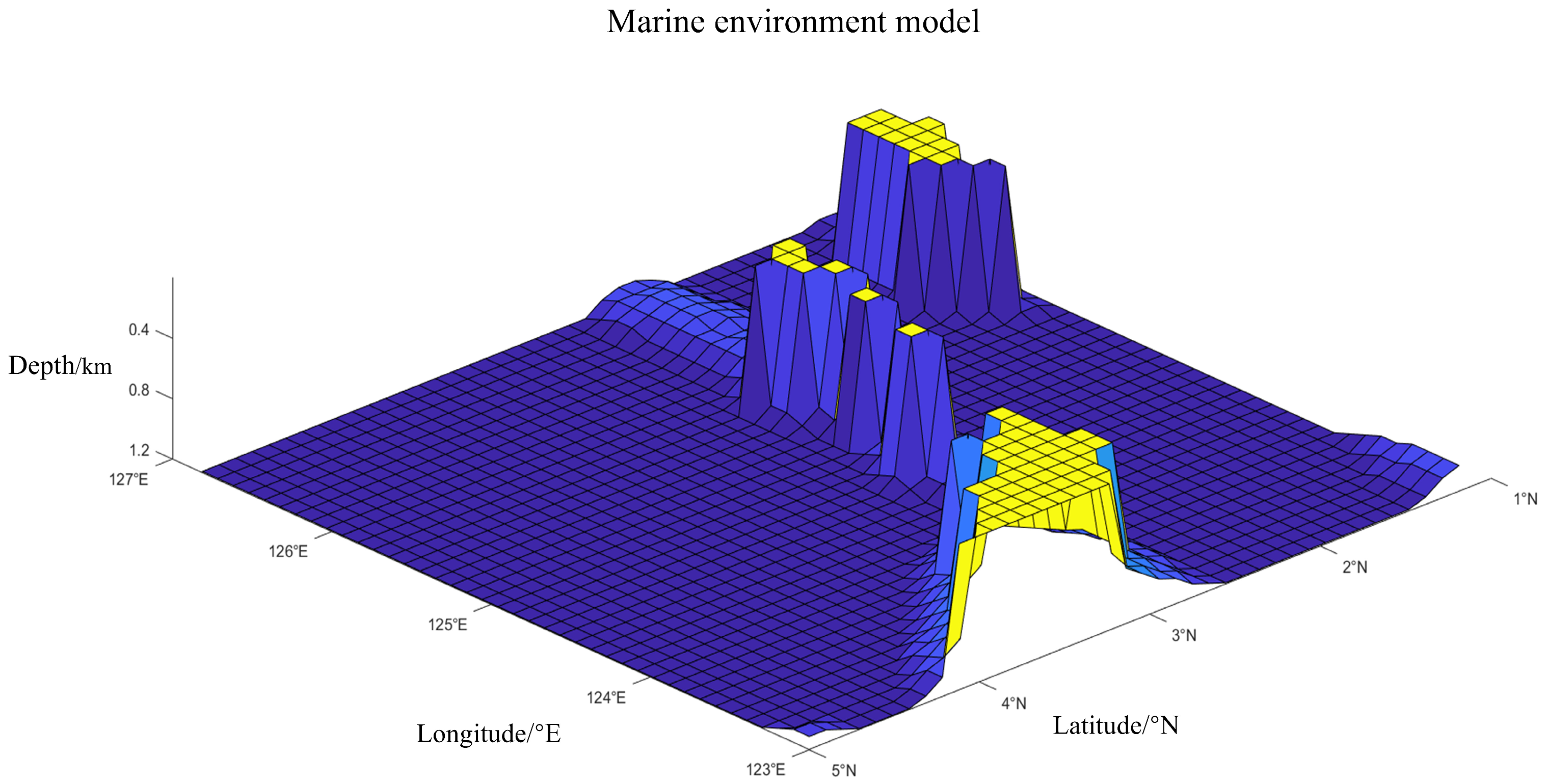
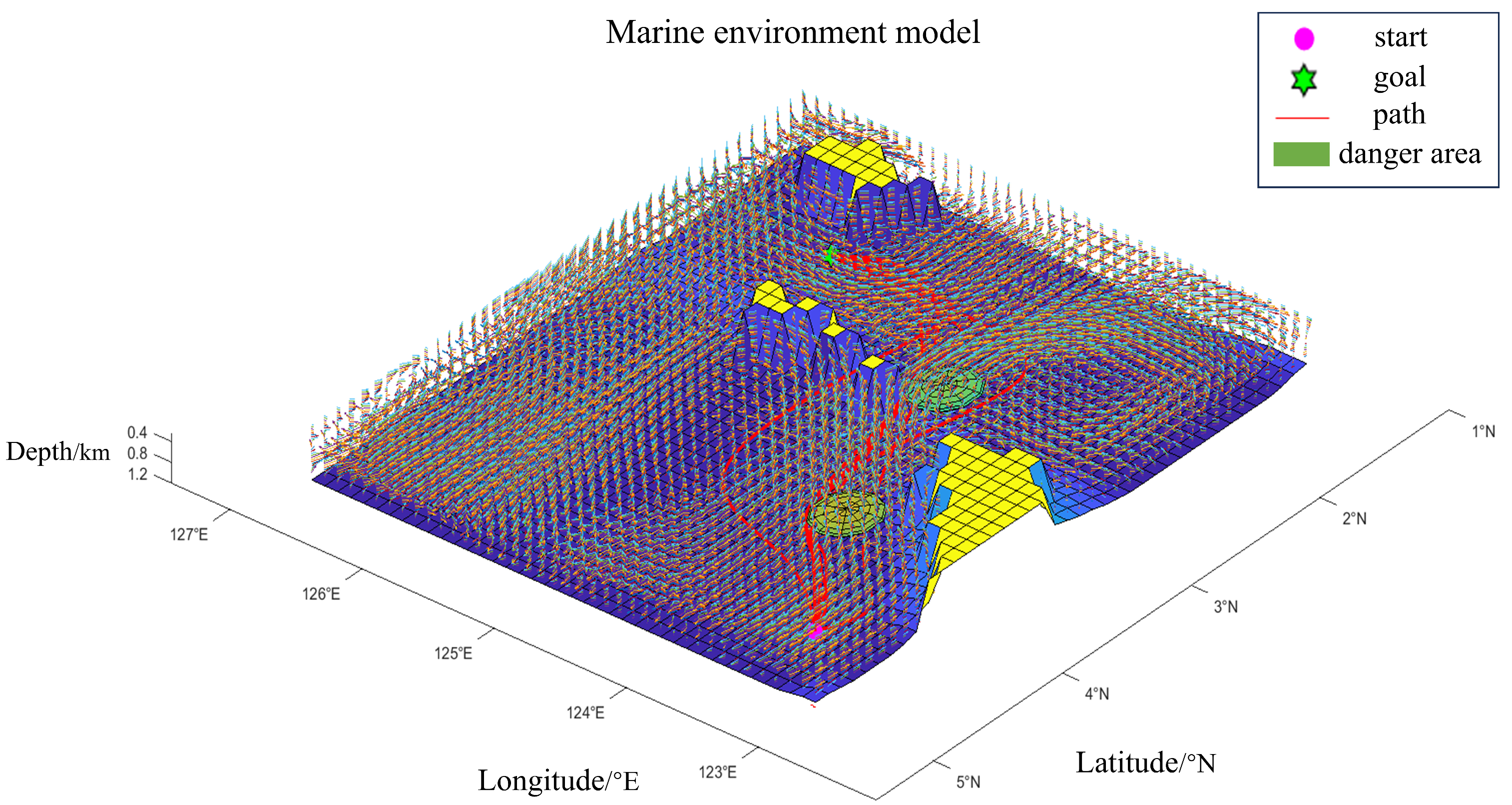
2.1. Three-Dimensional Marine Environment Model

Environmental modeling is essential for path planning. This study employed the raster method to construct an environment model, creating the raster maps from terrain and obstacle data in the planning area. The planning space was divided uniformly into the feasible and infeasible raster units, representing the terrain and obstacle coordinates in the three-dimensional space. The path planning focuses on optimizing the connections between the edge points of feasible raster units [25]. Figure 1 illustrates the three-dimensional raster map model.

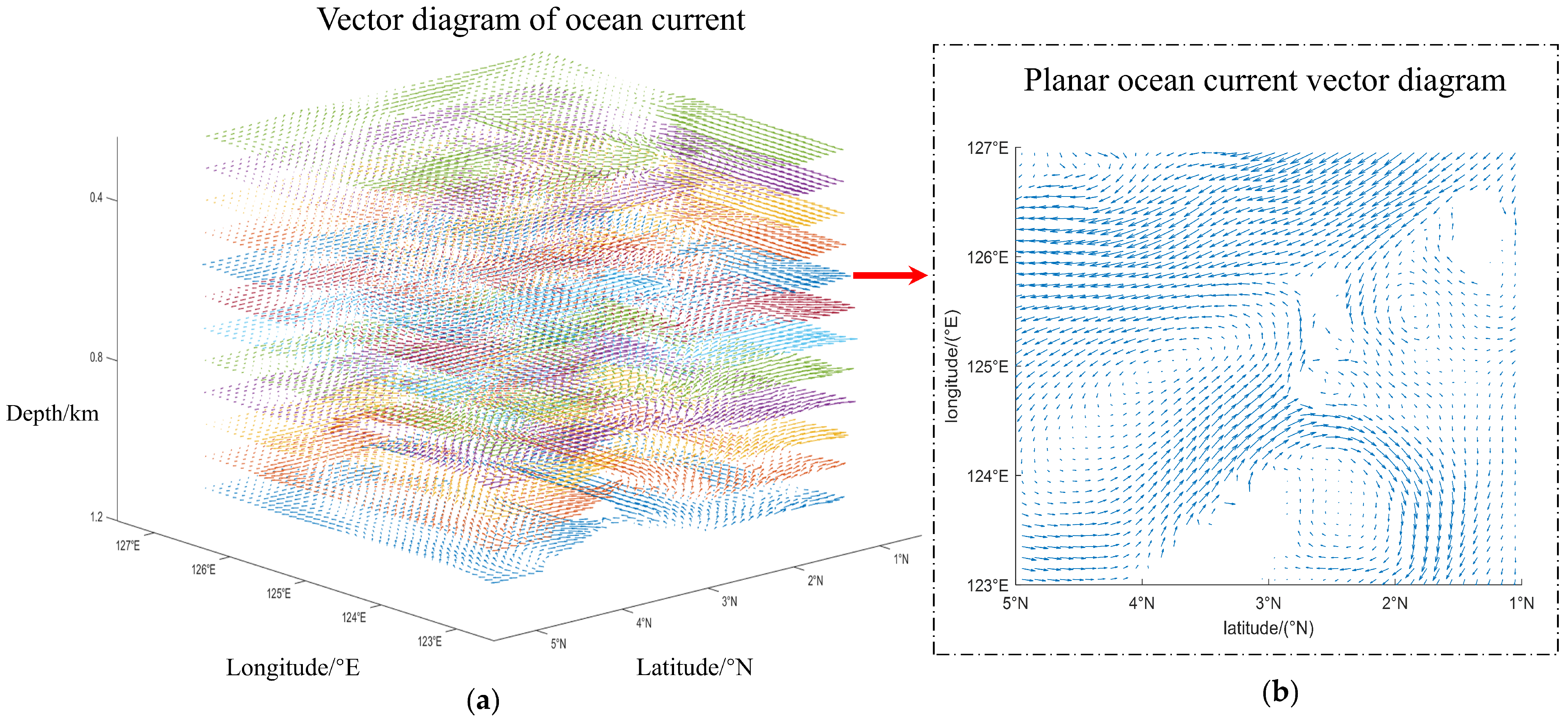
2.2. Representation of Three-Dimensional Ocean Current

These currents are widespread seawater flows in the ocean. To realistically represent the actual ocean environment, this study utilized the South China Sea ocean reanalysis product dataset [26] from the National Earth System Science Data Center, which included the real islands and conventional ocean physical variables over a specified period. Each layer of the current data consisted of two matrices: one storing the x-direction component and the other storing the y-direction component. The current environment, analyzed using MATLAB, is shown in Figure 2. The diagram on the left illustrates multi-level currents, whereas the right diagram shows one specific layer.
However, owing to equipment limitations and the complexity of the ocean environment, the accuracy of the current data observations was limited. Consequently, only one vector could approximate the current conditions within a specific range. Therefore, when assessing the influence of currents on AUVs, it could be essential to calculate the current velocity and direction as intervals. The vertical currents exerting the minimal influence were ignored. Let the current vector be c, the velocity magnitude in the horizontal direction be c v , the direction angle be c d , and ϕ and θ be the uncertainty levels of the current magnitude and direction angle. Subsequently, the upper- and lower-bound expressions of the current intervals are as follows:
c ν L = c ν ϕ c ν R = c ν + ϕ c d L = c d θ c d R = c d + θ
The intervals of velocity magnitude and direction of the currents are [ c ν L , c ν R ] and [ c d L , c d R ] , respectively.

2.3. Kinematic Modeling of the AUV

The kinematic model of an AUV included the translation and rotations [27]. We adopted both the equations of motion, and the equation can be represented as
η = ( x , y , z , σ , θ , φ )
τ = ( u , v , w , p , q , r )
where x , y , z are the positions of the AUV relative to north, east, down, or up, respectively; σ , θ , φ are the roll, pitch, and yaw, respectively; u , v , w are the reference velocity component in the direction of water fluctuation, sway, and heave, respectively; and p , q , r are the roll fetch, pitch fetch, and traverse rate, respectively. The linear velocity of the AUV significantly affected the sailing time, whereas the changes in the angular velocity indicated the energy consumed during steering, providing guidance for subsequent planning.
The velocity of the AUV relative to the geodetic coordinate system was the vector sum of the AUV’s propulsive velocity and ocean current velocity, expressed by the following equation [17]:
v g , i = v A U V + c
where v g , i , v A U V , c are the velocity of AUV to the ground, AUV propulsion velocity, and ocean current velocity, respectively.
The schematic of velocity synthesis is shown in Figure 3.

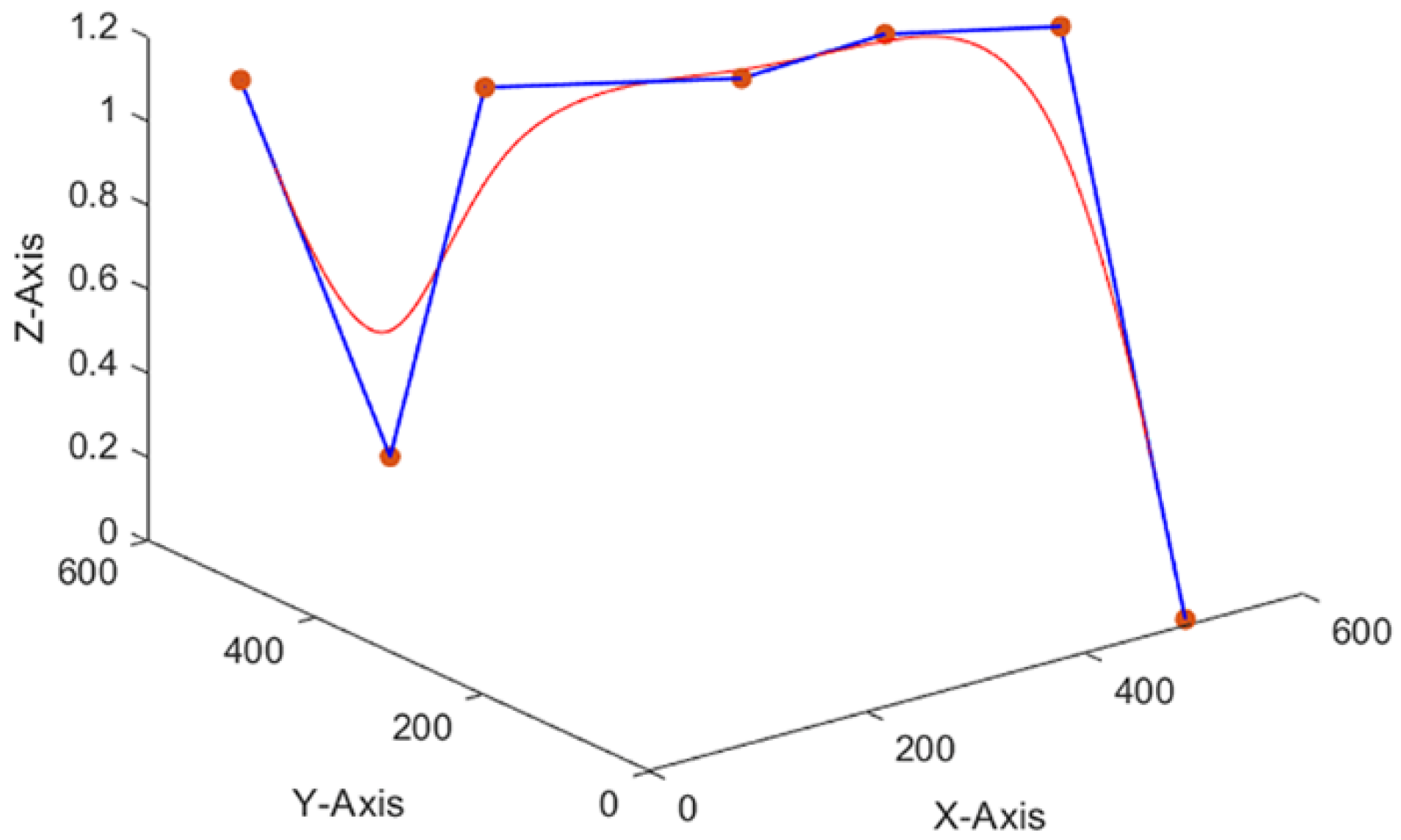
2.4. Path-Smoothing Processing

In the raster maps, constructing the underwater three-dimensional paths involved the application of B-spline curves. These curves required few control points to locally define the complex curvatures. The changes in the individual nodes did not significantly affect the overall curve, effectively fulfilling the path-planning requirements. The complete expression of B-spline curves was highly smooth within finite orders. However, it was inherently segmented, thereby overcoming the oscillation issue of Bezier curves. The expression for the B-spline curve is as follows [17]:
P ( u ) = i = 0 n   P i B i , k ( u ) , u [ u k 1 , u n + 1 ]
where P i is the individual control vertex, and B i , k ( u ) is called the kth order B-Spline basis function.
For path-smoothing in this research, we utilize cubic splines of order four. The control points comprise four intermediate points uniformly spaced between the start and end points, supplemented by the start and end points. Triple repetition of both the initial and terminal points guarantees exact interpolation at these locations, yielding a total of 10 control points.
Various types of B-spline curves existed depending on the node distribution. Due to the numerous benefits of the quasi-uniform B-spline curves and to expedite the computation, those curves were utilized for constructing three-dimensional paths [28], as depicted in Figure 4 Paths were defined by a sequence of control points on the B-spline curves, including the starting and ending points. Following the generation rules of the B-spline curves, the actual path points x 1 , x 2 , , x n can be computed using the equation, where x 1 and x n denote the starting and ending points of the path, respectively. The path Γ could be obtained by connecting them with a straight line. The expression is as follows:
Γ = { x 1 x 2 ¯ , x 2 x 3 ¯ , , x n 1 x n ¯ }

3. AUV Path-Planning Objective Function

In submarine environments, AUV navigation involves numerous constraints to ensure the feasibility of the planned path. This study considered the following constraints:
  • Seafloor terrain limitations: When navigating through current environments, underwater vehicles should maintain a height above the seafloor terrain to prevent collisions and avoid hazards.
  • The voyage minimizes time and energy consumption, and safe arrival at the destination is ensured.
According to the constraint analysis, underwater vehicle path planning presents a typical multi-objective constrained nonlinear optimization problem. The navigable path considered the navigation time cost of the underwater vehicle, uncertain obstacle constraints, ocean-current constraints, and path smoothness. The ocean currents primarily affected the velocity of the AUV relative to the geodetic coordinate system, combined with the propulsive velocity of the AUV. When incorporating the ocean-current constraints, they were converted into the navigation time-constraint costs. According to the kinematic model, the smoothness of the AUV path was related to its pitch and yaw angles. The smoother paths required less energy to adjust these angles.
Therefore, in this study, we employ the interval analysis method, taking the navigation time interval, danger degree interval, and path smoothness as the objective functions. The safety and timeliness were prioritized as the primary objectives in path planning, with path smoothness as a secondary objective. The optimization initially focused on these primary objectives, followed by the secondary screening of candidate paths. Section 3.1, Section 3.2 and Section 3.3 constructs three objective functions, namely, the voyage time interval, danger degree interval, and path smoothness.

3.1. Navigation Time Cost Interval

The time taken by the AUV to navigate along the route is the sum of the time taken at each path x i x i + 1 ¯ .
T = i = 1 n | x i x i + 1 ¯ | | v g , i |
where x i x i + 1 ¯ is the i-th segment of the path, and ν g , i is the velocity of the AUV with respect to the geodetic coordinate system.
Since the current vector was represented as an interval and the time taken by an AUV navigating within this interval current was uncertain, this study employed the mathematical analytical method to compute the interval of AUV navigation time within the interval current as T L , T R .

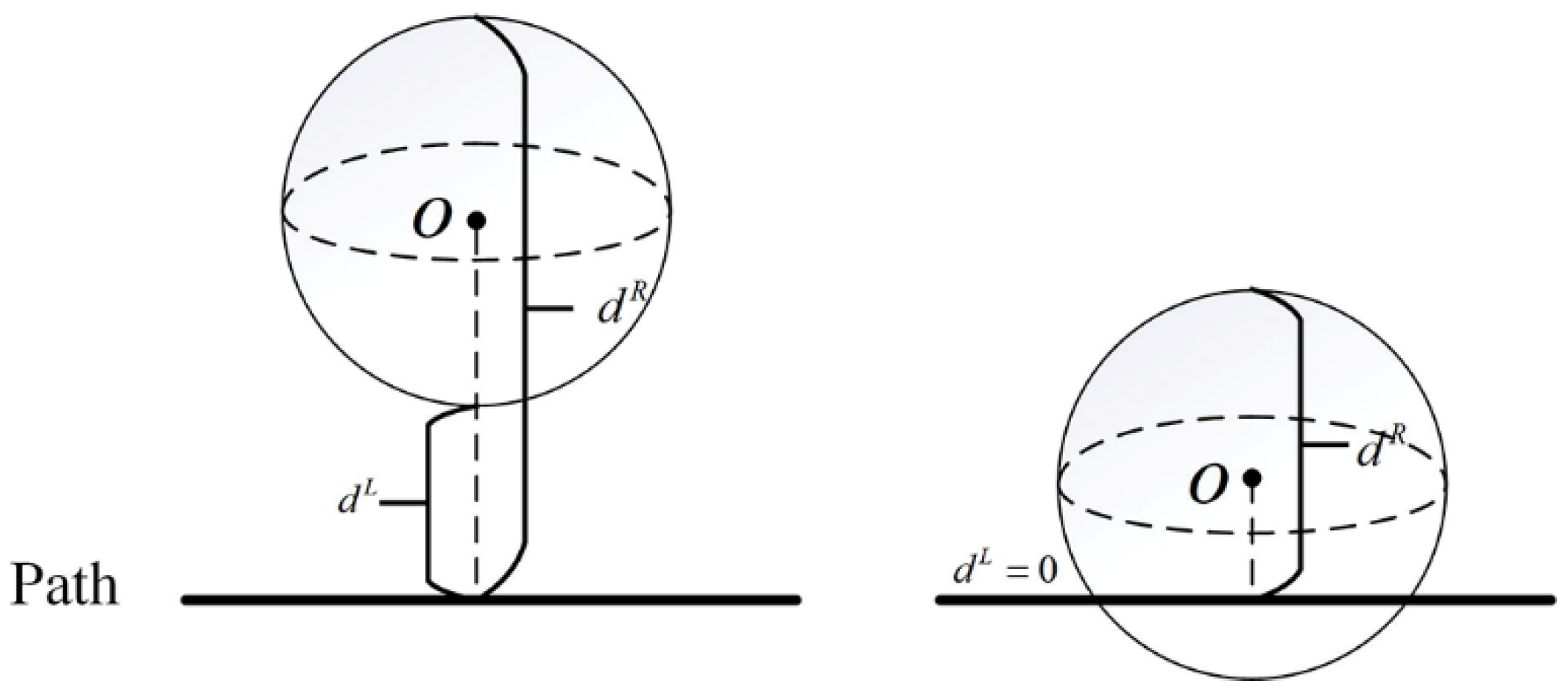
3.2. Uncertain Obstacle Constraint Cost Interval

When addressing the uncertain hazard sources, path planning should consider the distances between the path and these hazards. Interval numbers were applied to denote the uncertainty ranges of the sources. Figure 5 illustrates the maximum and minimum distances between the path and hazard sources in scenarios where the path intersected or did not intersect the uncertain range. The left side of the figure depicts the uncertainty range where the path avoided direct contact with hazard sources, and the right side presents the active area where the path intersected with hazard sources.
Let the activity range of the uncertain hazard source D i be inside the ball Ω i . If the center of the ball is Oi and the radius is ri, then the shortest distance from point pi on the path to the possible location of the source is
d L = d ( p i , O i ) r i , p i Ω i 0 , p i Ω i
The longest possible distance in both cases is
d R = d ( p i , O i ) + r i
The distance of the path from the hazard source can be obtained as an interval number [ d L , d R ].
When hazard avoidance was considered, a greater distance from the source was preferable. However, circumventing hazards may involve longer routes or navigation against the current. Therefore, in the calculations, the source was assigned an absolute danger distance lmin and a safety distance lmax. A path was considered hazardous if its distance from the hazard source was less than the absolute danger distance. If the distance exceeded lmax, the hazard source posed no threat to the path. Within these thresholds, the danger level decreased as the distance increased. The danger level of point p on a path relative to the i-th source Di could be calculated as follows [29]:
H i = 0 d ( p , D i ) > l max l max d ( p , D i ) l max l min l max > d ( p , D i ) > l min 1 d ( p , D i ) < l min
where d p , D i is the distance between the path point and the hazard source. From the above equation, the distance between the path point and the hazard source is an interval number [ d L , d R ], and the danger level H of a candidate path is the danger level of the point with the largest danger level on the path. Therefore, the danger level of the final calculated path is also an interval number [ H L , H R ].

3.3. Path Smoothness

The greater the smoothness of the AUV, the fewer the path corners, which could enhance the maneuverability and reduce the energy consumption during steering. The horizontal and vertical smoothness functions, P1 and P2, are defined as follows [30]:
P 1 = i = 1 d   a t a n 2 y i + 1 y i x i + 1 x i a t a n 2 y i y i 1 x i x i 1
P 2 = i = 1 d   a t a n 2 y i + 1 y i z i + 1 z i a t a n 2 y i y i 1 z i z i 1
a t a n 2 y x = a r c t a n y x x > 0 a r c t a n y x + π y 0 , x < 0 a r c t a n y x π y < 0 , x < 0 + π 2 y > 0 , x = 0 π 2 y < 0 , x = 0 undefined y = 0 , x = 0
where d is the total number of path points. x i , y i , and z i are the three-dimensional coordinate values of the i-th path point; x i + 1 , y i + 1 , and z i + 1 are the three-dimensional coordinate values of the (i + 1)-th path point; and x i 1 , y i 1 , and z i 1 are the three-dimensional coordinate values of the (i − 1)-th path point, respectively. a t a n 2 is the magnitude tangent function. Since P1 and P2 are independent of each other, the total smoothness can be weighted by P1 and P2.

4. AUV Path-Planning Based on IMOSBOA

The path-planning problem with multiple constraints is fundamentally a multi-objective optimization problem. Some scholars have linearly weighed these constraints to convert them into a single-objective optimization problem, where the selection of weights directly affects the planning results. This study employed non-dominated dominance ordering to depict the relationships between each objective function.

4.1. Dominance Relationship Based on the Interval Possibility Degree Model

Predominance occurred when an individual’s fitness surpassed that of another across all the objectives. Let Γ 1 and Γ 2 represent the time intervals affected by uncertain currents, with durations T 1 I = [ T 1 L , T 1 R ] and T 2 I = [ T 2 L , T 2 R ] , respectively, and radii of T 1 W and T 2 W , respectively. Equation (14) can be derived from the interval possibility degree model described in Reference [31]. P ( T 1 I T 2 I ) denotes the possibility degree that interval T 1 I exceeds the interval T 2 I ; specific comparisons of sailing time intervals proceed accordingly:
P ( T 1 I T 2 I ) = T 2 R T 1 L 2 T 1 W + 2 T 2 W
Similarly, the hazard levels for routes Γ 1 and Γ 2 are H 1 I = [ H 1 L , H 1 R ] and H 2 I = [ H 2 L , H 2 R ] , respectively. According to the interval possibility formula, the likelihood that the interval H 2 I is superior to the interval H 1 I is P ( H 1 I H 2 I ) . If there is [31]
P ( T 1 I T 2 I ) < P ( T 2 I T 1 I ) P ( H 1 I H 2 I ) < P ( H 2 I H 1 I )
then the route Γ 2 is better than the route Γ 1 in both adaptation intervals of sailing time and danger level, and Γ 2 is said to dominate Γ 1 .

4.2. Secretary Bird Optimization Algorithm

The secretary bird optimization algorithm is based on the behavior of secretary birds and employs two main strategies. The first strategy focuses on hunting and involves three phases: searching for, consuming, and attacking prey. The second strategy is dedicated to escaping predators and consists of the camouflage and evasion phases [19].

4.2.1. Secretary Bird Exploration Strategies

The entire predation process was divided into three equal time intervals, t < 1 3 T , 1 3 T t < 2 3 T , and 2 3 T t T , where t is the current iteration number and T is the total iteration number. During the first stage, a differential evolution strategy utilized the differences between individuals to generate new solutions, thereby enhancing the algorithmic diversity and global search capabilities. In the second stage, the concepts of historical best positions and Brownian motion were introduced, enabling individuals to conduct localized searches around previously identified optimal positions to explore the solution space more effectively. The third stage incorporated the Levy flight strategy to further boost the optimizer’s global search capabilities, mitigate the risk of falling into local solutions, and enhance the convergence accuracy.
x i , j n e w = x i , j + x r a n d o m 1 x r a n d o m 2 × R 1 , t < 1 3 T x b e s t + exp ( t / T ) 4 × ( R B 0.5 ) × x b e s t x i , j , 1 3 T t < 2 3 T x b e s t + 1 t T 2 × t T × x i , j × R L , 2 3 T t T
where t denotes the number of current iterations; T denotes the maximum number of iterations; x r a n d o m 1 and x r a n d o m 2 are random candidate solutions for the first stage iteration; R 1 denotes a randomly generated array of dimension 1 × Dim in the interval [0, 1]; Dim is the dimension of the solution space; x i , j n e w denotes the value of its j-th dimension; R B denotes a randomly generated array of dimension 1 × Dim from a standard normal distribution (mean 0, standard deviation 1); x b e s t is the current optimum; and R L is the Levy flight function multiplied by 0.5.

4.2.2. Secretary Bird Exploitation Strategies

When secretary birds detected the presence of a predator, they initially search for a suitable camouflaged environment. If no safe camouflage is available nearby, they either fly or run swiftly to escape. To deal with this situation, a dynamic perturbation factor is introduced, expressed as ( 1 t T ) 2 . This parameter can improve the global search ability in the early stage and the local approximation ability in the later stage. In summary, the two evasion strategies employed by secretary birds can be modeled as follows:
x i , j n e w = x b e s t + ( 2 × R B 1 ) × 1 t T 2 × x i , j , i f r a n d < r x i , j + R 2 × x r a n d o m K × x i , j , e l s e
where r = 0.5, R 2 denotes a randomly generated array of dimension 1 × Dim from a normal distribution, x r a n d o m denotes a random candidate solution for the current iteration, and K denotes a random choice of integer 1 or 2.

4.2.3. Improvement Approach

Like all other group optimization algorithms, SBOA is prone to fall into local optima after a certain number of iterations. As the number of iterations increases, the inferior individual will move closer to the gradually superior individual. In order to increase the diversity of solutions, this paper introduces a single point variation method [32] to increase the randomness of individual motion, so that the inferior individual has a certain probability to search in other directions. The specific method is to randomly select a control point with an infeasible path, and carry out a certain range of random changes to the coordinates of the control point. If we set the control point of the randomly selected path curve as b i = ( x i , y i , z i ) , then the mutation operation method is as follows:
x i = min x i + n o r m r n d μ , σ 2 , x m a x y i = min y i + n o r m r n d μ , σ 2 , y m a x z i = m i n ( z i + n o r m r n d ( μ , σ 2 ) , z m a x )
Since the random variation in the uniform distribution is likely to cause the path to become worse, this paper adopts the normal distribution method to generate random numbers, in which n o r m r n d is a random function, and the parameters in the random number function are the mean and variance of the normal distribution, respectively, and the position of the path points after variation does not exceed the boundary of the planning area.

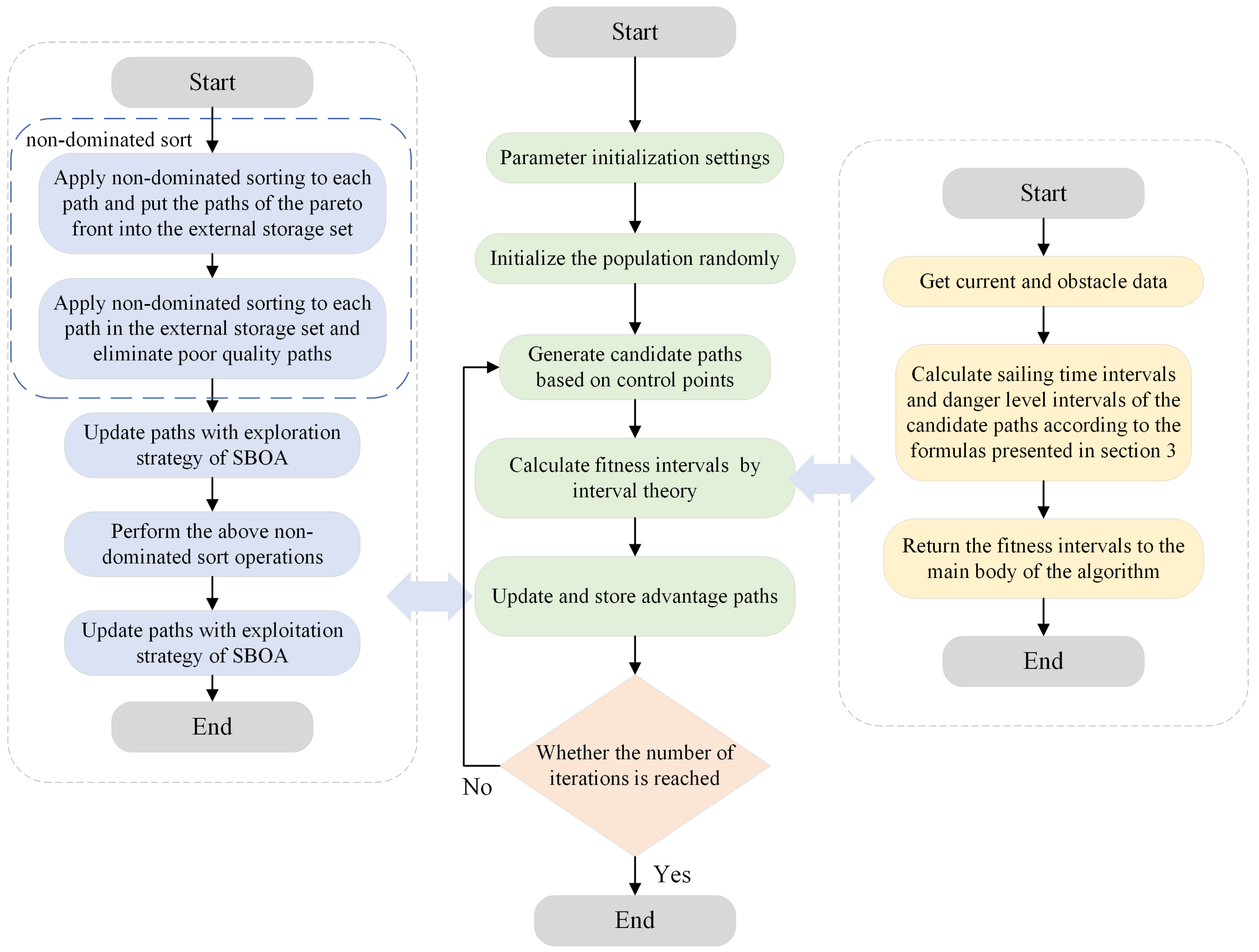
4.3. Interval Multi-Objective Path-Planning Algorithm

The problem of path planning in uncertain environments can be reformulated as an interval multi-objective optimization challenge. This study combined the enhanced interval predominance sorting algorithm with the secretary bird optimization algorithm to address multi-objective path planning under uncertain constraints. AUVs could face multiple navigational constraints, necessitating the application of a multi-objective optimization approach to achieve objectives such as minimizing navigation time and reducing danger. The interval-based Pareto dominance ranking method discussed earlier was integrated into the secretary bird optimization algorithm. An external storage set retained the individuals exhibiting the high dominance levels in each iteration, yielding a set of optimal paths. Finally, a smoothness criterion was applied to select the path with the highest smoothness from the optimal set as the optimal path.
The algorithm aimed to minimize the navigation cost of an underwater vehicle and identify the optimal path. This path was represented by a curve defined by a B-spline curve comprising a starting point, an end point, and four randomly positioned control points in space, treated collectively as an individual. The accessible area was defined as the feasible domain for each individual.
The pseudocode of the algorithm is shown in Algorithm 1, and a flowchart of the algorithm is shown in Figure 6.
Algorithm 1: IMOSBOA
1: Create 3D environmental model, including obstacles and currents.
2: Initialize problem setting, including the number of control points and individuals, maximum iteration (T), current iteration (t), and number of paths.
3: Initialize the population randomly and calculate the fitness intervals of each object.
4: For t = 1:T do
    Update each secretary bird’s best position.
    For each particle do
        Use exploration strategy to update secretary bird position according to Equation (16).
      Update each secretary bird’s best position.
      Do undominated sort for all individuals and put which ranks 1 into external storage set.
      Use exploitation strategy to update secretary bird position according to Equation (17).
      Update each secretary bird’s best position.
      Do undominated sort for all individuals and put which ranks 1 into external storage set.
    end
    Do undominated sort for all individuals in the external storage set.
    If the number of individuals in the external storage set exceeds the set value then
        Compare the Pareto levels and crowding distances of individuals and delete a certain number of individuals.
    end
    Use mutation operations to update disadvantaged individuals according to Equation (18).
  end
5: Calculate the smoothness of individuals in the external storage set and select the individual with the highest smoothness the optimal solution.
6: Output the optimal value (the optimal path).

5. Simulation Analysis

To validate the feasibility and effectiveness of the proposed algorithm in real marine environments, we first implemented an experimental simulation model of the algorithm in a marine environment. Subsequently, we conducted a series of simulation experiments using an Intel i7 7820HQ processor with a main frequency of 2.9 GHz, 16 GB of RAM, and the MATLAB R2023b environment.
This study utilized the South China Sea Ocean reanalysis dataset from the National Earth System Science Data Center, which contained the standard oceanic variables, such as the islands and currents. The marine environment data is in the format of a Net CDF file, which contains ocean current and terrain information within a certain range at a certain time point in the form of a four-dimensional vector. The four dimensions are the ocean current component of the x, y, and z axes and the time point, respectively, and the ocean floor topography where the ocean current component is NA. In this study, the ncread function in MATLAB is used to read the ocean current data of each coordinate and time, and the data is saved in a four-dimensional array. In environmental modeling, the selected area is set as a 40 × 40 × 24 3D raster map. The propulsion speed was set at 0.9 m/s. The current direction uncertainty σ d i r e c t was 10°, and the current magnitude uncertainty σ m a n g i was 0.05 m/s. The uncertain hazard source had a radius of 5 km, safety distance lmax of 20 km, and an absolute danger distance lmin of 2 km. The search area was defined as a square region from 1° N to 5° N and 123° E to 127° E. The voyage started at (1.25° N, 123.25° E) and ended at (3.91° N, 126.11° E). Based on a large number of simulation experiments, the optimal number of particles was determined to be 30, as this quantity provided the best balance between diversity and convergence speed. The results indicated that path adjustments tended to stabilize after 600 iterations. Therefore, 600 iterations were selected. When setting the convergence criterion, if the improvement in the optimal solution is less than 0.01% over 50 consecutive generations, the algorithm will be considered to have converged. This criterion aims to enhance the search efficiency of the algorithm. By evaluating whether there is no significant improvement in the optimal solution after several iterations, it indicates that the algorithm has converged to a local or global optimum. At this stage, further iterations yield diminishing returns, and the search results can effectively reflect the convergence behavior of the algorithm. In the first 1–200 iterations, the algorithm performs a rapid search, covering a wide solution space, but with a lower precision. Its focus is on identifying potential high-quality solution regions. In iterations 201–400, the focus shifts towards local optimization, with individuals conducting localized searches around the historical best positions using Brownian motion, thereby refining the solution quality. In iterations 401–600, the algorithm incorporates the Levy flight strategy, which allows it to explore previously unexplored areas of the solution space, helping to avoid local optima and enhancing convergence accuracy.

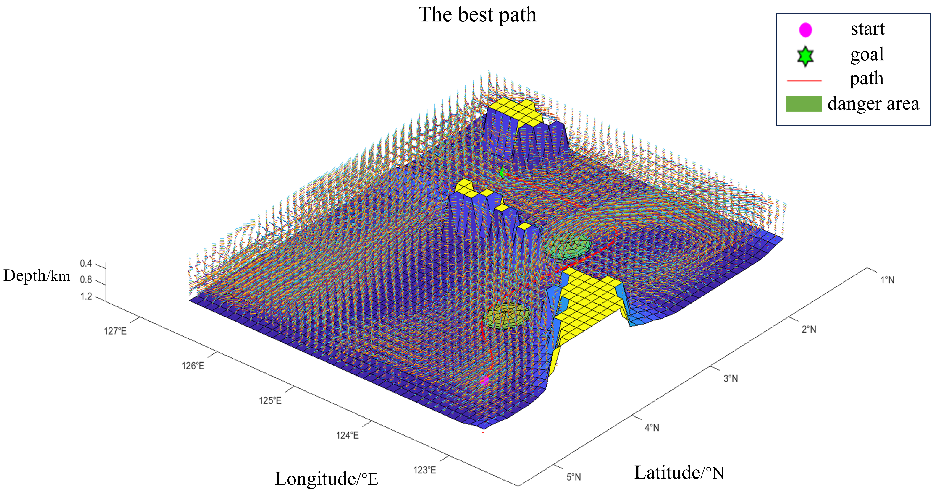
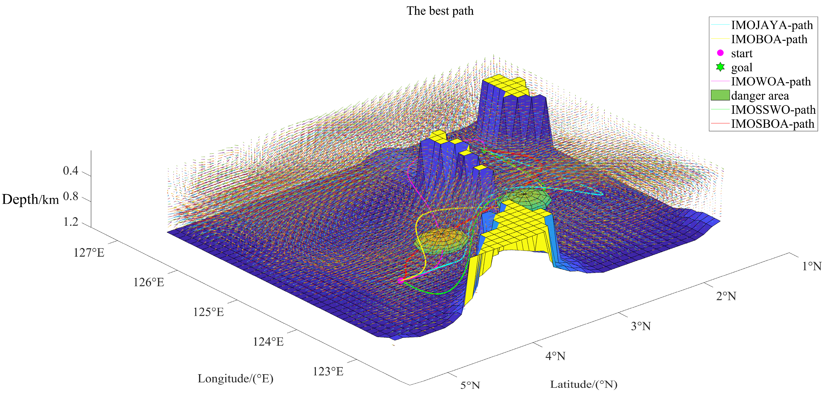
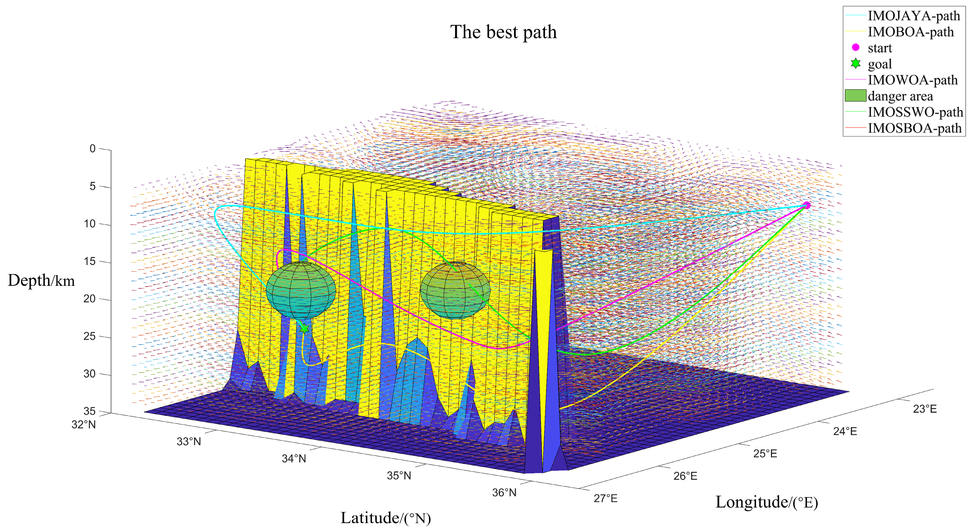
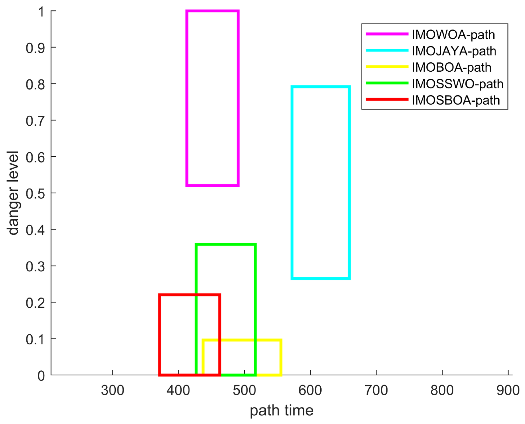
5.1. Comparison of Planning Results

Figure 7, Figure 8 and Figure 9 depict the planning results and Pareto fronts, respectively. The red curve represents the planned path, which generally aligns with the surface current flowing from the starting point to the target, albeit with a minor reverse current at the lower corner. At the starting point, the bottom current flowed in the opposite direction. Most paths followed the current direction, with the planned paths circumventing the first danger area located near a reverse current region on the map. The uncertain hazard source near the end point lay within the downward current area, leading most paths to traverse this region. The paths were evenly distributed, with the longest path circumventing all the hazard sources, while others were concentrated in areas with hazardous conditions and stronger currents, optimizing the time taken to reach the goal.
The specific fitness values for each path are depicted in Figure 9, with the danger level on the vertical axis and the navigation time on the horizontal axis. The Pareto front demonstrated a well-distributed range, with longer navigation times generally associated with lower hazards by avoiding uncertain hazard sources. The bottom path with no danger also had the longest minimum navigation time limit. Conversely, the path with the highest danger level exhibited the shortest navigation time, disregarding hazard sources, and none of the paths dominated the others. The danger levels across paths ranged from a minimum of 0 to a maximum of 0.7889, indicating that no path posed absolute hazards. When selecting the optimal path, the consideration of path smoothness was recommended.
To further illustrate the effects of planning, the navigation times and danger levels for all paths in the external reserve pool are shown in Table 1. The path length is the sum of the distances between each path point. The navigation time interval and danger level interval are obtained from the calculation formulas in Section 3.1 and Section 3.2, respectively, where the interval width is defined as the difference between the upper and lower bounds of the interval. The smoothness of the path is calculated using the formula presented in Section 3.3.
Table 1 shows that Path 3 spanned 477.1668 km in length, while its navigation time was shorter than that of Path 4, which covered only 464.5595 km. This discrepancy arose because the navigation time depended not only on the path length, but also on the utilization of ocean currents. The width of the navigation time interval was related to these currents, with the routes passing through heavily influenced areas experiencing increased uncertainty. Path 3, with the smallest lower limit of navigation time at 93.4112 × 10³ s, benefited from the sailing with the current, although it also faced the highest danger level owing to direct exposure to hazard sources. Path 1 that avoided all the hazard sources and benefited from the favorable currents was hazard-free, yet featured the longest navigation time at 531.9796 × 10³ s. Path 2, exhibiting a very low danger level, also had a longer maximum navigation time. Other paths represented a compromise between the danger level and the navigation time. Path 2, noted for its greatest smoothness, was selected as the optimal path for decision-making, which can save more energy for steering.
In order to further verify the performance of the optimization algorithm proposed in this study, we integrate individual update strategies of four single-objective optimization algorithms, namely the whale optimization algorithm (WOA) [33], JAYA algorithm [34], BOA, and SSWO, into the interval multi-objective optimization framework of this paper, and compare them with the IMOSBOA algorithm proposed in this paper in two different maps. Map 1 employs a three-dimensional cartographic representation of a specific sea area in the South China Sea, as previously described. Map 2 utilizes a topographical depiction of the surrounding waters in Mediterranean, focusing on the strait of Antikythera, which was defined as a square region from 32° N to 36° N and 23° E to 27° E. The voyage started at (35.7° N, 23.25° E) and ended at (32.92° N, 25.85° E). Each algorithm used 30 populations and ran 600 iterations. The non-inferior solutions from all five algorithms were assessed against the optimal solution identified using the smoothness function. Figure 10 and Figure 11 present the partial planning results obtained using these algorithms. Figure 12 and Figure 13 and Table 2 and Table 3 shows the Pareto fronts of these five different algorithms.
In Map 1, the data in Table 2 highlighted that the IMOWOA planned a path of 498.3725 km with the maximum navigation time of 490.4883 × 10³ s, demonstrating time efficiency compared to several other algorithms. However, it achieved this at the cost of safety, with the danger levels ranging from 0.5201 to 1. As can be seen from Figure 10, this path passes through the hazard source, greatly increasing the probability of collision between the AUV and the danger sources. This may be because IMOWOA prioritizes path length and time efficiency during the optimization process, resulting in insufficient avoidance of hazard sources and consequently increasing the risk levels. In contrast, IMOJAYA planned a longer path of 598.5563 km with the longer navigation time and no significant safety advantage. As depicted in Figure 10, the path is more curved at the end, which is due to the influence of currents. IMOJAYA may lack adaptability to ocean currents, leading to path irregularities, which in turn increases the total path length and time cost. Both IMOBOA and IMOSSWO made a compromise between the danger levels and navigation times. IMOSBOA demonstrated remarkable improvements in navigation time, path danger level, and path length. Specifically, the average navigation time interval of IMOSBOA is reduced by 11.2% compared to IMOSSWO, highlighting its superior path-planning efficiency. Regarding the path danger level, while IMOSBOA’s value is slightly higher than that of IMOBOA, it remains significantly lower than those of both IMOWOA and IMOJAYA, showcasing its balanced advantage in safety. For path length, IMOSBOA generates a path of 468.0104 km, which is approximately 2.44% shorter than IMOSSWO (479.7072 km) and about 21.8% shorter than IMOJAYA (598.5563 km), further affirming its outstanding performance in path optimization.
In Map 2, the experimental results of the five algorithms reveal distinct performance characteristics. As summarized in Table 3, IMOJAYA prioritizes safety with a consistently maintained danger level of [0, 0], effectively avoiding hazardous areas. However, this safety advantage comes at a significant cost to efficiency, as evidenced by the longest path length of 762.6046 km among the five algorithms and a navigation time interval of [803.1691, 873.0247]. As illustrated in Figure 11, the path deviates substantially from the target direction to circumvent all hazardous areas, resulting in a considerable increase in both navigation time and path length. IMOWOA generates a path with a length of 642.1754 km and a navigation time interval of [623.9901, 681.0871], reflecting moderate time efficiency. However, the danger level interval of [0, 0.6395] suggests that the planned path traverses certain hazardous areas. From the visualization, it is evident that this path passes directly through some high-risk zones, thereby compromising safety to a certain extent. IMOBOA achieves a relatively short path length of 604.2674 km, demonstrating high spatial efficiency, but its danger level interval of [0.4824, 1] indicates substantial exposure to risk. Similarly, IMOSSWO, with a path length of 629.9831 km, exhibits a danger level interval spanning [0, 1], reflecting variable risk levels along the planned trajectory. IMOSBOA achieves the shortest path length of 614.4075 km with a navigation time interval of [587.0511, 622.3068], demonstrating remarkable time efficiency. Additionally, it maintains a low danger level interval of [0.1724, 0.6904], reflecting a well-balanced performance across navigation time, path length, and safety. Compared to IMOSSWO, IMOWOA, and IMOJAYA, IMOSBOA’s navigation time interval is reduced by approximately 6.43%, 7.99%, and 26.7%, respectively, highlighting its outstanding efficiency in path planning. In terms of the path danger level, although IMOSBOA’s interval is slightly higher than that of IMOJAYA, it is significantly lower than those of IMOWOA, IMOBOA, and IMOSSWO, further showcasing its balanced advantage in safety.
Overall, IMOSBOA outperforms the other algorithms in terms of navigation time, safety, and path length. As illustrated in the figure, this algorithm effectively leverages favorable environmental conditions, such as water currents, to facilitate efficient progress while avoiding obstacles. These results highlight the robust performance of IMOSBOA in addressing the multi-objective path-planning problem. The superior performance of IMOSBOA largely stems from the symmetrical search strategy: The exploration phase and exploitation phase form a symmetric balance in spatial search. In early iterations, extensive exploration avoids local optima. Later, localized exploitation refines paths (e.g., Phase 3: Levy flight enables large jumps to escape stagnation). The symmetric search strategy of IMOSBOA enables it to adapt to complex three-dimensional uncertain environments. The experimental results intuitively prove that this algorithm can efficiently coordinate ocean current utilization and danger avoidance.
The comparative results in Table 2 and Table 3 demonstrate that while IMOSBOA achieves a superior planning performance, this comes at the cost of increased computational time relative to simpler iterative approaches such as IMOJAYA. This computational overhead stems fundamentally from the algorithm’s sophisticated search strategy, which leads to a slight increase in the computing time of the algorithm.

5.2. Robustness Analysis

To further validate the effectiveness of the interval algorithm, it was compared with the conventional multi-objective optimization algorithm that did not account for the uncertainty. Initially, the precise sea-current measurements were performed without the uncertainty, and the hazard source radius was set to 0. The path planning was conducted using the multi-objective secretary bird algorithm (MOSBOA), and the results are presented in Table 4 and Figure 14, Figure 15 and Figure 16. The minimum navigation time achieved under deterministic sea current and hazard source conditions was 345.9630 × 10³ s, which exceeded the minimum navigation time in Table 1. However, the maximum navigation time of 367.1387 × 10³ s was significantly lower than that observed under uncertain conditions (531.9796 × 10³ s). Furthermore, the maximum danger level (0.2304) was lower than that listed in Table 1. These outcomes resulted from the increased uncertainty during planning under uncertain conditions.
The planning results of the interval multi-objective optimization algorithm proposed in this study were compared with the paths planned without considering uncertainty. We randomly generated the 1000 planning scenarios within the current and hazard source uncertainty intervals using a normal distribution. The mean values represented the measured values, and variance followed the 3σ principle, which was set to 1/3 of the uncertainty range for the currents and hazard sources. On this basis, we use the formulas in Section 3.1 and Section 3.2 to set the uncertainty as 0 to calculate the navigation times and danger levels of paths and select the maximum and minimum values. The variance is the variance of the value of the navigation times and the danger levels for 1000 tests of the path. The results of the navigation times and danger levels for paths planned by the proposed algorithm and a conventional multi-objective algorithm in stochastic environments are presented in Table 5 and Table 6, respectively. At the same time, we investigate the impact of uncertainty on the feasibility of the planned path. Specifically, we consider directional uncertainties of 5°, 10°, and 20°, as well as amplitude uncertainties of 0.05 m/s, 0.1 m/s, and 0.15 m/s. Simulations are conducted to evaluate the performance of two algorithms in these marine environments. From the Pareto fronts generated by the two algorithms, we select the paths with the best smoothness for a detailed comparison. The simulation results are shown in Table 7.
Below, we compare the sum of the maximum navigation times and the sum of the minimum navigation times for the seven paths listed in the above table, as well as the sum of the maximum and minimum danger levels. Firstly, in terms of navigation time, although traditional multi-objective optimization algorithms reduced the minimum navigation time by an average of 12.7% compared to the proposed IMOSBOA algorithm, IMOSBOA exhibited a smaller difference between its maximum and minimum navigation times in random environments, with the maximum navigation time being significantly lower than that of MOSBOA. This indicates a degree of stability, suggesting that IMOSBOA can more effectively address the uncertainties in ocean currents and reduce the risk of extreme delays in challenging environments. In contrast, MOSBOA, which does not consider environmental uncertainties, resulted in some paths with infinite navigation times, meaning that these paths may become impassable due to uncertain currents and hazard sources, severely compromising their practical feasibility.
Secondly, the comparison of danger levels further highlights the robustness advantage of IMOSBOA. The danger levels of IMOSBOA paths showed less fluctuation in random environments and remained within a lower range, with only two alternative paths having a maximum danger level exceeding 0.5. This performance is attributed to IMOSBOA’s comprehensive modeling and optimization of the uncertainties in the activity ranges of the hazard sources. On the other hand, MOSBOA, which neglects the uncertainty of hazard sources and lacks proactive planning, produced paths with higher danger levels in multiple tests. Some paths even reached a danger level of 1, rendering them infeasible. The average increases in the maximum and minimum danger levels for MOSBOA-planned paths were 137.7% and 31.9%, respectively, reflecting its inadequacy in addressing variations in hazard source locations and ranges.
Thirdly, in terms of path feasibility, IMOSBOA achieved full possibility in all random tests, demonstrating excellent reliability, while MOSBOA showed infeasible paths in 3% of the tests. As we can see in Table 7, the data reveals significant differences in the infeasibility frequency of path planning between the IMOSBOA and MOSBOA algorithms under various uncertainty conditions. With small directional uncertainty (5°), both IMOSBOA and MOSBOA are able to avoid infeasible paths entirely, regardless of the amplitude uncertainty (0.05 m/s, 0.1 m/s, or 0.15 m/s), demonstrating strong adaptability. However, when the directional uncertainty increases to 10°, the infeasibility frequency of MOSBOA rises sharply from 0 to 54 as the amplitude uncertainty increases from 0.05 m/s to 0.15 m/s, whereas IMOSBOA’s infeasibility frequency only increases from 0 to 3, showing a clear advantage of IMOSBOA under moderate uncertainty. In high directional uncertainty (20°), MOSBOA’s infeasibility frequency increases dramatically with increasing amplitude uncertainty, from 87 to 275, while IMOSBOA’s infeasibility frequency remains relatively low, increasing from 5 to 20, demonstrating superior robustness in high-uncertainty environments. Overall, IMOSBOA consistently shows a significantly lower infeasibility frequency than MOSBOA, especially under high directional and amplitude uncertainties, reflecting its excellent stability and reliability. In contrast, MOSBOA is more sensitive to uncertainty, with its performance degrading exponentially as uncertainty increases. Therefore, IMOSBOA is better suited for complex marine environments with high uncertainty, while MOSBOA is more suitable for scenarios with low uncertainty. By converting uncertain parameters into interval bounds, the interval dominance relationship directly incorporates worst-case scenarios. This transforms environmental uncertainty into quantifiable optimization constraints, explaining IMOSBOA’s 0% infeasibility rate and thereby ensuring its robustness.
In summary, by fully considering the randomness and uncertainty of ocean currents and hazard sources during the planning phase, IMOSBOA achieves robust path planning. This capability not only reduces fluctuations in navigation time and danger levels but also significantly enhances the practical feasibility of the paths, demonstrating a high degree of robustness.

6. Conclusions

This study proposed IMOSBOA for the three-dimensional path planning of AUVs, designed to address multiple uncertain constraints in the AUV navigational environments. The algorithm enhanced the traditional intelligent optimization methods by introducing fitness-interval calculations and comparisons. It integrated the iterative strategy of the secretary bird optimization algorithm with a non-dominated dominance ranking algorithm to effectively handle uncertain planning environments. Using the interval possibility model, the algorithm managed the uncertainty constraints, enabling the multi-objective path planning in unpredictable environments. By optimizing fitness interval computations and leveraging non-dominated dominance sorting, the algorithm generated a well-distributed set of feasible paths, from which the optimal path was selected based on the smoothness criteria. The simulation experiments validated the effectiveness of the algorithm in environments with uncertain currents and hazard sources, demonstrating its ability to plan multiple viable paths with the improved distribution. Compared with conventional multi-objective optimization algorithms ignoring the uncertainty, this algorithm exhibited higher reliability in uncertain marine environments with multiple constraints. IMOSBOA has improved feasibility over MOSBOA by approximately 74.12% under several uncertainty conditions.
In conclusion, the proposed algorithm successfully achieves the two main research objectives. First, by integrating interval theory, it effectively addresses the uncertainty in AUV path planning caused by fluctuating ocean currents and unpredictable hazardous sources, ensuring the robustness of the path in complex marine environments. Second, experimental results using real-world maps demonstrate that the algorithm consistently generates stable, safe, and efficient three-dimensional paths, outperforming traditional methods in terms of stability, safety, and efficiency. These results validate its practical applicability in uncertain ocean conditions. Overall, the algorithm effectively handles uncertainty constraints and delivers efficient path-planning solutions.
However, the global path-planning algorithm proposed in this paper cannot be directly applied in practice due to the challenge of obtaining real-time marine environment data over a large area. This limitation is further compounded by the simplifying assumptions made during simulations, such as constant AUV speed and idealized current models, which may not fully capture the dynamic complexities of real-world marine environments. In our future research, we will address the issue of path planning in the absence of accurate real-time marine environmental data. It is a feasible scheme to combine global path planning and local path replanning with a two-layer planning structure. Firstly, the algorithm proposed in this paper is used for global path planning based on marine environmental data in a specific time range, and then combined with local path planning in actual operation. Specifically, real-time environmental data is sampled from the AUV’s sensors and reprogrammed using a sampling-based algorithm. Common local path replanning methods include the Dynamic Window Method (DWA) and Model Predictive Control (MPC). This method greatly improves the feasibility of the application of the algorithm in the actual marine environment.

Author Contributions

Conceptualization, L.Q. and T.N.; methodology, C.L., J.S. and R.T.; software, D.Z. and Y.L.; validation, J.G. (Jiajun Gong) and J.G. (Jia Guo); formal analysis, J.S., H.L. and Y.L.; data curation, J.G. (Jia Guo) and S.Y.; writing—original draft preparation, S.Y. and R.T.; writing—review and editing, R.T. and J.G. (Jiajun Gong); visualization, T.N., D.Z. and C.L.; supervision, H.L. and L.Q.; project administration, Y.L. and H.L. All authors have read and agreed to the published version of the manuscript.

Funding

This work was supported by the National Natural Science Foundation of China (Grant No. 62441308).

Data Availability Statement

The original contributions presented in this study are included in the article, and further inquiries can be directed to the corresponding author.

Acknowledgments

The authors would like to thank all the reviewers who participated in the review.

Conflicts of Interest

The authors Tian Ni, Jia Guo, Huan Liu, and Yushan Li are employed by the company China Ship Scientific Research Center. The remaining authors declare that the research was conducted in the absence of any commercial or financial relationships that could be construed as a potential conflict of interest.

References

  1. Wang, L.; Zhu, D.; Pang, W.; Zhang, Y. A survey of underwater search for multi-target using Multi-AUV: Task allocation, path planning, and formation control. Ocean Eng. 2023, 278, 114393. [Google Scholar] [CrossRef]
  2. Yan, Z.; Li, Y. Data collection optimization of ocean observation network based on AUV path planning and communication. Ocean Eng. 2023, 282, 114912. [Google Scholar] [CrossRef]
  3. Wu, Y. Coordinated path planning for an unmanned aerial-aquatic vehicle (UAAV) and an autonomous underwater vehicle (AUV) in an underwater target strike mission. Ocean Eng. 2019, 182, 162–173. [Google Scholar] [CrossRef]
  4. Zeng, Z.; Lian, L.; Sammut, K.; He, F.; Tang, Y.; Lammas, A. A survey on path planning for persistent autonomy of autonomous underwater vehicles. Ocean Eng. 2015, 110, 303–313. [Google Scholar] [CrossRef]
  5. Auh, E.; Kim, J.; Joo, Y.; Park, J.; Lee, G.; Oh, I.; Pico, N.; Moon, H. Unloading sequence planning for autonomous robotic container-unloading system using A-star search algorithm. Eng. Sci. Technol. Int. J. 2024, 50, 101610. [Google Scholar] [CrossRef]
  6. Sedeño-Noda, A.; Colebrook, M. A biobjective Dijkstra algorithm. Eur. J. Oper. Res. 2019, 276, 106–118. [Google Scholar] [CrossRef]
  7. Kulkarni, C.S. Three-Dimensional Time-Optimal Path Planning in Dynamic and Realistic Environments. Master’s Thesis, Massachusetts Institute of Technology, Cambridge, MA, USA, 2017. Available online: http://hdl.handle.net/1721.1/111730 (accessed on 15 January 2024).
  8. Hadi, B.; Khosravi, A.; Sarhadi, P. Deep reinforcement learning for adaptive path planning and control of an autonomous underwater vehicle. Appl. Ocean Res. 2022, 129, 103326. [Google Scholar] [CrossRef]
  9. Tang, Z.; Cao, X.; Zhou, Z.; Zhang, Z.; Xu, C.; Dou, J. Path planning of autonomous underwater vehicle in unknown environment based on improved deep reinforcement learning. Ocean Eng. 2024, 301, 117547. [Google Scholar] [CrossRef]
  10. Yao, X.; Wang, F.; Wang, J.; Wang, X. Optimal time path planning for underwater robots in uncertain current environments. Control Theory Appl. 2020, 37, 1302–1310. Available online: https://jcta.ijournals.cn/cta_cn/ch/reader/create_pdf.aspx?file_no=CCTA190273&flag=1&journal_id=cta_cn&year_id=2020 (accessed on 15 January 2024).
  11. Zhao, J.; Deng, C.; Yu, H.; Fei, H.; Li, D. Path planning of unmanned vehicles based on adaptive particle swarm optimization algorithm. Comput. Commun. 2024, 216, 112–129. [Google Scholar] [CrossRef]
  12. Cui, Y.; Hu, W.; Rahmani, A. Multi-robot path planning using learning-based artificial bee colony algorithm. Eng. Appl. Artif. Intell. 2024, 129, 107579. [Google Scholar] [CrossRef]
  13. Li, G.; Liu, C.; Wu, L.; Xiao, W. A mixing algorithm of ACO and ABC for solving path planning of mobile robot. Appl. Soft Comput. 2023, 148, 110868. [Google Scholar] [CrossRef]
  14. Zhang, W.; Wang, N.; Wu, W. A hybrid path planning algorithm considering AUV dynamic constraints based on improved A* algorithm and APF algorithm. Ocean Eng. 2023, 285, 115333. [Google Scholar] [CrossRef]
  15. Huang, H.; Wen, X.; Niu, M.; Miah, M.S.; Wang, H.; Gao, T. Multi-Objective Path Planning of Autonomous Underwater Vehicles Driven by Manta Ray Foraging. J. Mar. Sci. Eng. 2024, 12, 88. [Google Scholar] [CrossRef]
  16. Zhan, B.; An, S.; He, Y.; Wang, L. Three-Dimensional Path Planning for AUVs Based on Standard Particle Swarm Optimization Algorithm. J. Mar. Sci. Eng. 2022, 10, 1253. [Google Scholar] [CrossRef]
  17. Li, X.; Yu, S. Three-dimensional path planning for AUVs in ocean currents environment based on an improved compression factor particle swarm optimization algorithm. Ocean Eng. 2023, 280, 114610. [Google Scholar] [CrossRef]
  18. Benmamoun, Z.; Khlie, K.; Bektemyssova, G.; Dehghani, M.; Gherabi, Y. Bobcat Optimization Algorithm: An Effective Bio-Inspired Metaheuristic Algorithm for Solving Supply Chain Optimization Problems. Sci. Rep. 2024, 14, 20099. [Google Scholar] [CrossRef]
  19. Fu, Y.; Liu, D.; Chen, J.; He, L. Secretary bird optimization algorithm: A new metaheuristic for solving global optimization problems. Artif. Intell. Rev. 2024, 57, 1–102. [Google Scholar] [CrossRef]
  20. Abdel-Basset, M.; Mohamed, R.; Sallam, K.M.; Elsayed, S. Efficient algorithms for optimal path planning of unmanned aerial vehicles in complex three-dimensional environments. Knowledge-Based Syst. 2025, 316, 113344. [Google Scholar] [CrossRef]
  21. Yan, Z.; Zhao, Y.; Chen, T.; Chi, D. UUV path planning under imprecise navigation information. J. Harbin Eng. Univ. 2016, 34, 715–720. Available online: https://kns.cnki.net/kcms2/article/abstract?v=C4JADW50D8s1hinXkUZ97bX3anrmFYfaH23Ol6exB1K9ryYMxrbYSuPB_wb_QdPyy9XTipAK9myKiPDdftpYPEIJBQgXSz6cienHrEqvfGvBNaBfVE--nwldTCckIS_Fj4qtZBkWkEu6BVDTjzgJozIXxPQOgUT7i7Go7-oUEkz3aY3KA49CBg==&uniplatform=NZKPT&language=CHS (accessed on 15 January 2024).
  22. Li, B.; Chiong, R.; Lin, M. A two-layer optimization framework for UAV path planning with interval uncertainties. In Proceedings of the 2014 IEEE Symposium on Computational Intelligence in Production and Logistics Systems (CIPLS), Orlando, FL, USA, 9–12 December 2014; IEEE: New York, NY, USA, 2014; pp. 120–127. [Google Scholar]
  23. Yao, X.; Wang, F.; Yuan, C.; Wang, J.; Wang, X. Path planning for autonomous underwater vehicles based on interval optimization in uncertain flow fields. Ocean Eng. 2021, 234, 108675. [Google Scholar] [CrossRef]
  24. Shen, C.; Shi, Y.; Buckham, B. Integrated path planning and tracking control of an AUV: A unified receding horizon optimization approach. IEEE/ASME Trans. Mechatron. 2016, 22, 1163–1173. [Google Scholar] [CrossRef]
  25. Garrido, S.; Moreno, L.; Lima, P.U. Robot formation motion planning using fast marching. Robot. Auton. Syst. 2011, 59, 675–683. [Google Scholar] [CrossRef]
  26. National Earth System Science Data Sharing Platform. Scientific Data Center for the South China Sea and Adjacent Sea Areas. 2024. Available online: https://mds.nmdis.org.cn/pages/home.html (accessed on 15 June 2024).
  27. Li, D.; Luo, K.; Dang, J.; Wang, Y.; Zhang, Y. Kinematics and dynamics modeling of super-vacuum underwater vehicles. Syst. Eng. Theory Pract. 2013, 22, 2437–2442. Available online: https://sysengi.cjoe.ac.cn/CN/10.12011/1000-6788(2013)9-2437 (accessed on 15 January 2024).
  28. Zeng, Z.; Sammut, K.; He, F.; Lammas, A. Efficient path evaluation for AUVs using adaptive B-spline approximation. In Proceedings of the 2012 Oceans, Hampton Roads, VA, USA, 14–19 October 2012; IEEE: New York, NY, USA, 2012; pp. 1–8. [Google Scholar]
  29. Zhang, Y. Particle Swarm Optimization Theory and Application to Interval Multi-Objective Optimization Problems. Ph.D. Thesis, China University of Mining and Technology, Jiangsu, China, 2009. Available online: https://kns.cnki.net/kcms2/article/abstract?v=WYPw_9jmhsJ08KKY_p1h5c8hH_dt7sQMK2Qgp8TnkzsXD5wSnfOF7zq1-fxix8vpINggLDot1JN6kDysz7_4J-hhj8NigUMGkHwdRaq7Lwdeo3cm0XXfFC6QB5PawIY49erFT9_M2juP8HTj2hwvJmCFQuknIxxh&uniplatform=NZKPT&language=CHS (accessed on 15 January 2024).
  30. Guo, X.; Ji, M.; Zhang, W.; Zhang, J.; Lingrui, K. Improved QPSO algorithm for dynamic path planning of autonomous underwater vehicles in variable ocean current environment. Syst. Eng. Theory Pract. 2021, 41, 2112–2124. [Google Scholar] [CrossRef]
  31. Jiang, C.; Han, X.; Xie, H. Theory and Methods of Optimal Design with Interval Uncertainty; Science Press of China: Beijing, China, 2017. [Google Scholar]
  32. Kim, S.; Noh, Y. Optimizing and Visualizing Drone Station Sites for Cultural Heritage Protection and Research Using Genetic Algorithms. Systems 2025, 13, 435. [Google Scholar] [CrossRef]
  33. Mirjalili, S.; Lewis, A. The whale optimization algorithm. Adv. Eng. Softw. 2016, 95, 51–67. [Google Scholar] [CrossRef]
  34. Rao, R. Jaya: A simple and new optimization algorithm for solving constrained and unconstrained optimization problems. Int. J. Ind. Eng. Comput. 2016, 7, 19–34. [Google Scholar] [CrossRef]
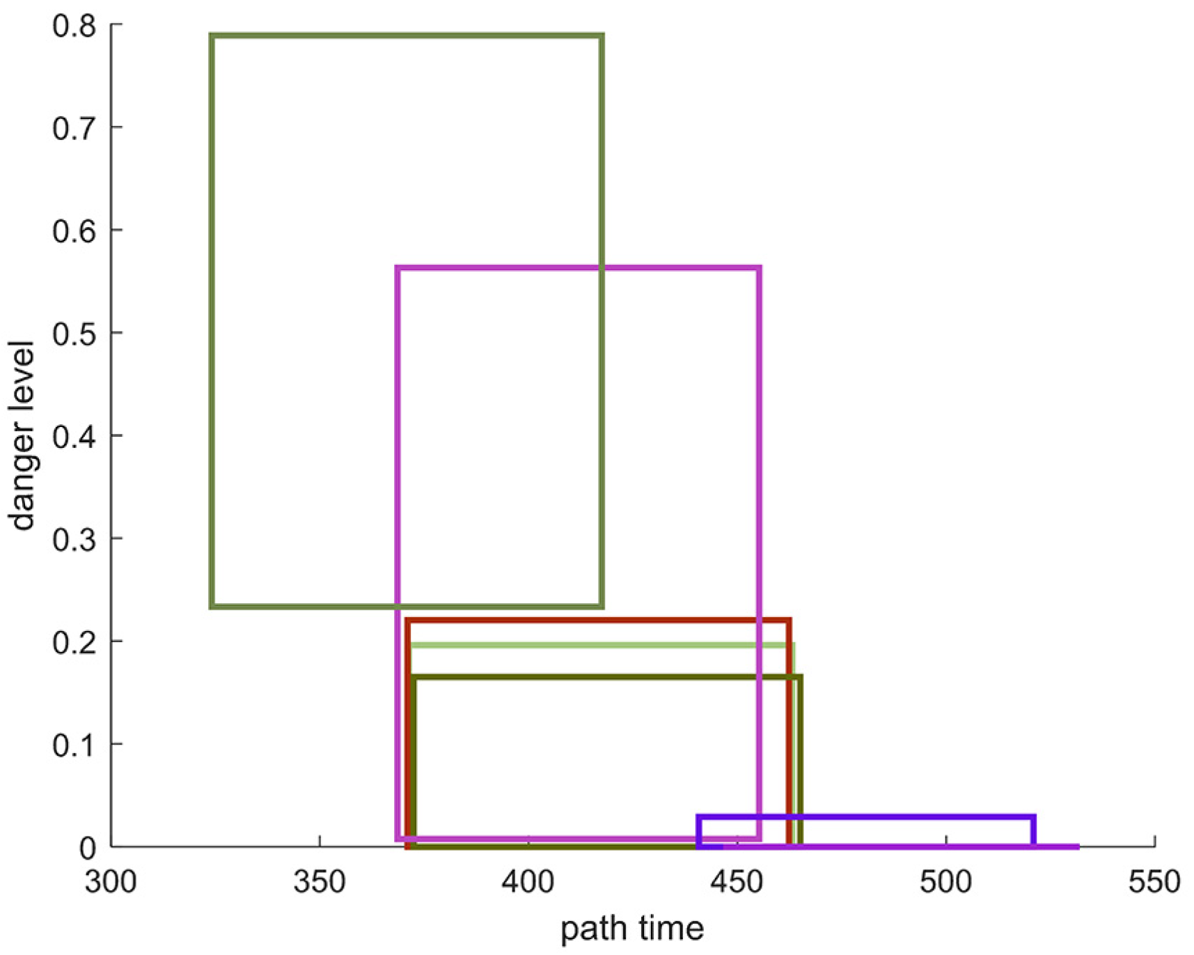
Figure 1. Three-dimensional raster map model.
Symmetry 17 00993 g001
Figure 2. Visualization of ocean current data, showing (a) multi-level current patterns and (b) a specific layer’s current vectors.
Symmetry 17 00993 g002
Figure 3. Schematic diagram of AUV velocity synthesis.
Symmetry 17 00993 g003
Figure 4. Quasi-uniform cubic B-spline curve.
Symmetry 17 00993 g004
Figure 5. Relationship between paths and uncertain hazard sources.
Symmetry 17 00993 g005
Figure 6. Algorithm flowchart.
Symmetry 17 00993 g006
Figure 7. Map of planning results of IMOSBOA.
Symmetry 17 00993 g007
Figure 8. The best path of IMOSBOA.
Symmetry 17 00993 g008
Figure 9. Pareto front of IMOSBOA.
Symmetry 17 00993 g009
Figure 10. Planning results of five different methods in Map 1.
Symmetry 17 00993 g010
Figure 11. Planning results of five different methods in Map 2.
Symmetry 17 00993 g011
Figure 12. Pareto fronts of five different algorithms in Map 1.
Symmetry 17 00993 g012
Figure 13. Pareto fronts of five different algorithms in Map 2.
Symmetry 17 00993 g013
Figure 14. Map of planning results of MOSBOA.
Symmetry 17 00993 g014
Figure 15. The best path of MOSBOA.
Symmetry 17 00993 g015
Figure 16. Pareto front of MOSBOA.
Symmetry 17 00993 g016
Table 1. The algorithm in this paper plans the resulting data.
PathPath Length/kmNavigation Time Interval/103sDanger Level IntervalSmoothness
1500.9485[446.6056, 531.9796][0, 0]10.9812
2492.8639[440.7722, 520.9105][0, 0.0291]11.5765
3477.1668[324.0923, 417.5034][0.2333, 0.7889]2.4798
4464.5595[368.5957, 455.2428][0.0075, 0.5631]10.2770
5467.4834[372.4773, 465.0564][0, 0.1651]10.4107
6468.0104[371.0080, 462.3871][0, 0.2204]11.0351
7468.3167[371.2707, 463.1554][0, 0.1961]10.4973
Table 2. Planning results of the five algorithms in Map 1.
AlgorithmNavigation Time Interval/103 sDanger Level IntervalPath Length/kmComputing Time/s
IMOWOA[412.5829, 490.4883][0.5201, 1]498.372561.23
IMOJAYA[572.0301, 658.7970][0.2651, 0.7914]598.556339.41
IMOBOA[437.1723, 555.1822][0, 0.0962]547.708156.15
IMOSSWO[426.7163, 516.3460][0, 0.3589]479.707257.54
IMOSBOA[371.0080, 462.3871][0, 0.2204]468.010453.31
Table 3. Planning results of the five algorithms in Map 2.
AlgorithmNavigation Time Interval/103 sDanger Level IntervalPath Length/kmComputing Time/s
IMOWOA[623.9901, 681.0871][0, 0.6395]642.175466.12
IMOJAYA[803.1691, 873.0247][0, 0]762.604642.43
IMOBOA[592.7619, 646.0583][0.4824, 1]604.267459.21
IMOSSWO[619.6304, 672.3713][0, 1]629.983164.12
IMOSBOA[587.0511, 622.3068][0.1724, 0.6904]614.407557.41
Table 4. Algorithm in this study used for planning resulting data.
PathPath Length/kmNavigation Time/103 sDanger Level Smoothness
1458.0690355.02830.015110.5530
2483.1942345.96300.230410.5788
3471.0274366.13260.013910.3139
4490.9841367.138706.8358
5457.0748349.16570.033910.5089
6457.0778349.14840.033410.5088
7456.0678348.13280.033910.4975
Table 5. Random test results of the paths obtained by IMOSBOA.
PathNavigation Time/103 sDanger LevelInfeasible Frequency
MinMax.VarianceMinMax.Variance
1454.4884461.70780.98080000
2394.8548400.48090.768000.16240.00270
3385.0747389.55810.611800.16690.00300
4380.2231384.72940.535900.35150.00950
5369.2018374.43850.685000.37590.00780
6362.6054366.59720.40890.06310.53990.00680
7365.2121369.34680.42180.06390.50440.01010
Table 6. Random test results of the paths obtained by MOSBOA.
PathNavigation Time/103 sDanger LevelInfeasible Frequency
MinMax.VarianceMinMax.Variance
1353.1453-00.19960.00419
2339.7723-0.02480.43210.00625
3337.6752341.78150.431000.29110.00460
4359.9571-010.008023
5324.5049328.35860.31180.11780.62120.01070
6325.7989330.01940.36750.02800.41720.00510
7325.8614329.21050.31650.13130.53340.00530
Table 7. Random test results with different uncertainties.
UncertaintyInfeasible Frequency
sdirect (◦)smangi (m/s)IMOSBOAMOSBOA
50.0500
50.100
50.1500
100.0500
100.1021
100.15354
200.05587
200.19132
200.1520275
Disclaimer/Publisher’s Note: The statements, opinions and data contained in all publications are solely those of the individual author(s) and contributor(s) and not of MDPI and/or the editor(s). MDPI and/or the editor(s) disclaim responsibility for any injury to people or property resulting from any ideas, methods, instructions or products referred to in the content.

