Well-Posedness of Cauchy-Type Problems for Nonlinear Implicit Hilfer Fractional Differential Equations with General Order in Weighted Spaces

Abstract

This paper establishes the well-posedness of Cauchy-type problems with non-symmetric initial conditions for nonlinear implicit Hilfer fractional differential equations of general fractional orders in weighted function spaces. Using fixed-point techniques, we first prove the existence of solutions via Schaefer’s fixed-point theorem. The uniqueness and Ulam–Hyers stability are then derived using Banach’s contraction principle. By introducing a novel singular-kernel Gronwall inequality, we extend the analysis to Ulam–Hyers–Rassias stability and continuous dependence on initial data. The theoretical framework is unified for general fractional orders and validated through examples, demonstrating its applicability to implicit systems with memory effects. Key contributions include weighted-space analysis and stability criteria for this class of equations.

1. Introduction

Fractional differential equations (FDEs) generalize classical differential equations by allowing derivatives of non-integer order, offering a robust framework for describing complex systems with memory and hereditary characteristics. The foundations of fractional calculus date back to the 17th century, notably through correspondence between Gottfried Wilhelm Leibniz and Guillaume de L’Hôpital, where the idea of non-integer-order derivatives was first discussed. Since then, the theory has been systematically advanced by prominent mathematicians including Joseph Liouville, Bernhard Riemann, Hermann Weyl, and Marcel Riesz.

In contemporary research, fractional calculus has emerged as a powerful tool in diverse fields of science and engineering. Its ability to model nonlocal and history-dependent behaviors makes FDEs especially effective in capturing the dynamics of systems characterized by anomalous diffusion and long-range temporal dependencies. As a result, they have been successfully applied to problems in physics, biology, control theory, economics, and engineering; see [1,2,3,4,5].

Research on FDEs parallels the theory of classical ordinary differential equations (ODEs), focusing on three fundamental problems: the existence of solutions, the uniqueness of solutions, and stability analysis. These questions constitute the core of the well-posedness problem, ensuring mathematical rigor in modeling.

The existence of solutions to FDEs is a foundational aspect that guarantees the mathematical viability of these models. Researchers have employed various techniques—such as fixed point theory—to establish both the existence and uniqueness of solutions under specific conditions. For instance, recent studies have shown that classical mathematical methods can effectively address the challenges posed by fractional derivatives, thereby enhancing our understanding of these equations; see the monographs [6,7].

In addition to existence results, the stability of solutions is another crucial area of investigation. Various stability concepts have been developed, each suited to different types of perturbations and modeling scenarios. In the context of FDEs, notions such as Lyapunov stability, asymptotic stability, Mittag–Leffler stability, and Ulam stability are commonly used, as they play a vital role in assessing how small perturbations in the initial conditions or parameters of FDEs affect the behavior of solutions over time.

Recently, researchers have shown great interest in Ulam-type stability concepts such as Ulam–Hyers stability, Ulam–Hyers–Rassias stability, and their generalizations; see [8,9,10,11,12] and the references cited therein. These stability frameworks not only provide insight into the robustness of solutions but also facilitate the development of numerical methods for solving fractional differential equations.

Overall, the exploration of existence and stability in fractional differential equations represents a rich field of research that bridges theoretical mathematics with practical applications. As researchers continue to uncover new results and methodologies, the implications for modeling real-world systems become increasingly profound, underscoring the importance of this area within the broader context of fractional calculus.

Various types of fractional derivatives have been introduced, among which the Riemann–Liouville fractional derivative and the Caputo fractional derivative are the most widely used. The Hilfer fractional derivative was introduced by Rudolf Hilfer in 1996. This derivative is notable for its two-parameter family, which generalizes both the Caputo and Riemann–Liouville fractional derivatives. The Hilfer derivative allows for interpolation between these two well-known definitions of fractional derivatives, providing greater flexibility in applications. It has spurred extensive research on Hilfer-type FDEs, as exemplified below:

Furati et al. [13] investigated the existence of solutions for Hilfer fractional differential equations with fractional integral initial conditions, given by

$$\left\{\begin{array}{cc}{\displaystyle D_{a^{+}}^{\alpha ,\beta }x\left(t\right)}\hfill & =f(t,x(t\left)\right),t\in (a,b],\hfill \\ I_{a^{+}}^{1-\gamma }x\left(a\right)\hfill & =x_a,\gamma =\alpha +\beta (1-\alpha ),\hfill \end{array}\right.$$

where $D_{a^{+}}^{\alpha ,\beta }$ is the Hilfer fractional derivative of order $\alpha \in (0,1)$, type $\beta \in [0,1]$, $I_{a^{+}}^{1-\gamma }$ is the Riemann–Liouville fractional integral of order $1-\gamma$, and $f:(a,b]\times \mathbb{R}\to \mathbb{R}$ is a given function. They proved the existence and uniqueness of global solutions in the space of weighted continuous functions. The stability of the solution for a weighted Cauchy-type problem is also analyzed.

Dhaigude et al. [14] studied the existence and uniqueness of solutions for Hilfer fractional differential equations involving Hilfer fractional derivatives with fractional integral initial conditions, given by

$$\left\{\begin{array}{cc}{\displaystyle D_{a^{+}}^{\alpha ,\beta }x\left(t\right)}\hfill & =f(t,x(t\left)\right),t\in (a,b],\hfill \\ I_{a^{+}}^{k-\gamma }x\left(a\right)\hfill & =b_k,k\in \{1,2,\dots ,n\},\hfill \end{array}\right.$$

where $D_{a^{+}}^{\alpha ,\beta }$ is the Hilfer fractional derivative of order $\alpha \in (n-1,n)$ and type $\beta \in [0,1]$; $I_{a^{+}}^{k-\gamma }$ is the Riemann–Liouville fractional integral of order $k-\gamma$, with $\gamma =\alpha +\beta (n-\alpha )$; and $f:(a,b]\times \mathbb{R}\to \mathbb{R}$ is a given function.

In 2018, Vivek et al. [15] studied the existence, uniqueness, and stability of solutions for an implicit differential equation with a nonlocal condition involving the Hilfer fractional derivative, given by

$$\left\{\begin{array}{c}{D}_{0^{+}}^{\alpha ,\beta }x\left(t\right)=f(t,x\left(t\right),D_{0^{+}}^{\alpha ,\beta }x\left(t\right)),t\in J=[0,T],\hfill \\ I_{0^{+}}^{1-\gamma }x\left(0\right)=\sum _{i=1}^m{c}_{i}x\left({\tau }_i\right),\alpha \le \gamma =\alpha +\beta (1-\alpha )<1,{\tau }_i\in [0,T],\hfill \end{array}\right.$$

where $D_{0^{+}}^{\alpha ,\beta }$ is the Hilfer fractional derivative with $\alpha \in (0,1)$ and $\beta \in [0,1]$ and $f:J\times \mathbb{R}\times \mathbb{R}\to \mathbb{R}$ is a given continuous function. The operator $I_{0^{+}}^{1-\gamma }$ denotes the left-sided Riemann–Liouville fractional integral of order $1-\gamma$. The coefficients $c_i$ are real constants, and the points ${\tau }_i$ for $i=1,2,\dots ,m$ are fixed such that $0<{\tau }_1\le {\tau }_2\le \dots \le {\tau }_m<T$.

Motivated by the ongoing research on Hilfer fractional differential problems, this paper establishes the existence, uniqueness, and stability of solutions in weighted function spaces for a class of nonlinear implicit Hilfer FDEs:

$$\begin{array}{c}\hfill D_{a^{+}}^{\alpha ,\beta }x\left(t\right)=f(t,x\left(t\right),D_{a^{+}}^{\alpha ,\beta }x\left(t\right)),t\in (a,b],a\ge 0,\end{array}$$

(1)

subject to the initial conditions

$$\begin{array}{c}\hfill x_{n-\gamma }^{(n-k)}\left(a\right)=c_k,c_k\in \mathbb{R},k\in \{1,2,\dots ,n\},\end{array}$$

(2)

where $D_{a^{+}}^{\alpha ,\beta }$ denotes the Hilfer fractional derivative of order $\alpha \in (n-1,n)$ and type $\beta \in [0,1]$. The operator ${(·)}_{n-\gamma }^{(n-k)}:=D^{n-k}{I}_{a^{+}}^{n-\gamma }(·)$, where $D^{n-k}$ is the standard derivative of integer order $n-k$ and $I_{a^{+}}^{n-\gamma }$ denotes the Riemann–Liouville fractional integral of order $n-\gamma$, with $\gamma =\alpha +\beta (n-\alpha )$. Here, $f:(a,b]\times \mathbb{R}\times \mathbb{R}\to \mathbb{R}$ is a given function.

We employ fixed-point theorems to establish the existence and uniqueness of solutions while developing a generalized Gronwall inequality with singular kernels to investigate both continuous dependence on initial data and stability properties—particularly Ulam–Hyers stability and its variants. Concrete examples are presented to demonstrate the applicability of these theoretical results.

The class of nonlinear implicit Hilfer FDEs with general fractional order, considered in this paper, has broad applicability in modeling complex dynamical systems with memory and hereditary properties. Such equations naturally arise in physical and engineering systems where the current state depends not only on the present input but also on a nonlinear relationship involving the fractional derivative of the unknown function. A representative application can be found in viscoelastic materials, where the stress–strain relationship incorporates both time-fractional behavior and implicit constitutive laws. The implicit nature of the general fractional-order Equation (1) enables the modeling of feedback mechanisms or damping forces that depend on both the state and its rate of change, expressed through the Hilfer derivative.

Additionally, such implicit Hilfer FDEs are relevant in systems biology, anomalous transport processes in porous media, and fractional electrical circuits with memory-dependent components. In each of these cases, ensuring the existence, uniqueness, and stability of solutions is essential for the mathematical soundness and predictive power of the model. The results established in this paper—framed in weighted function spaces—provide a theoretical foundation for the analysis and simulation of such real-world systems.

The importance of weighted function spaces lies in their ability to capture the singular behavior often exhibited by solutions of fractional differential equations, particularly near boundary points. These spaces enable finer control over regularity and integrability properties, which is essential when working with fractional operators that involve singular kernels or nonlocal effects. As such, they are indispensable tools in establishing well-posedness and stability results in the fractional calculus framework.

The remainder of this paper is organized as follows. Section 2 introduces fundamental definitions, notations, and preliminary results, including the generalized Hilfer fractional derivative and the relevant solution spaces. Section 3 presents our main theoretical contributions, featuring a novel integral inequality with singular kernels. Section 4 establishes existence and uniqueness results for solutions. In Section 5, we investigate Ulam–Hyers-type stability concepts, encompassing classical, generalized, Rassias, and generalized Rassias stability. Section 6 examines continuous dependence on initial data, while Section 7 provides illustrative examples demonstrating the applicability of our theoretical framework. Section 8 discusses the broader implications of our results, and Section 9 concludes the paper with final remarks.

2. Preliminaries

2.1. Definitions and Lemmas

In this section, we present fundamental definitions and lemmas. Let $-\infty <a<b<\infty$, and let $L^1[a,b]$ denote the space of Lebesgue integrable functions, and $C[a,b]$ the space of continuous functions on $[a,b]$. For $n\in \mathbb{N}$ and $0\le \gamma <1$, we define the following weighted spaces of continuous functions:

$$C_{\gamma }[a,b]=\left\{{h:(a,b]\to \mathbb{R}|(t-a)}^{\gamma }h\left(t\right)\in C[a,b]\right\},$$

which means $h\left(t\right)$ may have a singularity at $t=a$, controlled by ${(t-a)}^{-\gamma }$ and

$$C_{\gamma }^n[a,b]=\left\{h\in C^{n-1}[a,b]|D^{n}h\in C_{\gamma }[a,b]\right\},$$

where $D^n:={\left({\displaystyle \frac{d}{dt}}\right)}^n$, with norms

$${\parallel h\parallel }_{C_{\gamma }[a,b]}={\parallel {(t-a)}^{\gamma }h\parallel }_{C[a,b]},$$

and

$${\parallel h\parallel }_{C_{\gamma }^n[a,b]}=\sum _{k=0}^{n-1}\parallel D^k{h\parallel }_{C[a,b]}+{\parallel D^{n}h\parallel }_{C_{\gamma }[a,b]}.$$

These spaces satisfy the following properties:

• $C_0[a,b]=C[a,b]$, $C_{\gamma }^0[a,b]=C_{\gamma }[a,b]$, and $C_0^n[a,b]=C^n[a,b],$
• $C[a,b]\subseteq C_{{\gamma }_1}[a,b]\subset C_{{\gamma }_2}[a,b]$ and $C^n[a,b]\subset C_{{\gamma }_1}^n[a,b]\subset C_{{\gamma }_2}^n[a,b]$ for $0\le {\gamma }_1<{\gamma }_2<1,$
• $C_{\gamma }^n[a,b]\subseteq C_{\gamma }[a,b]\subset L^1[a,b].$

Fractional calculus extends traditional integration and differentiation to non-integer orders, with foundational work by Riemann and Liouville in the 19th century.

Definition 1 

(Riemann–Liouville fractional integral [2]). For a function $h\in L^1[a,b]$, the left-sided Riemann–Liouville fractional integral of order $\alpha >0$ is defined as

$$I_{a^{+}}^{\alpha }h\left(t\right):={\displaystyle \frac{1}{\mathrm{\Gamma }\left(\alpha \right)}}{\int }_a^t{(t-\tau )}^{\alpha -1}h\left(\tau \right)d\tau ,t>a$$

where Γ is the Gamma function defined by

$$\mathrm{\Gamma }\left(z\right)={\int }_0^{\infty }{t}^{z-1}{e}^{-t}dz,z>0.$$

When $\alpha =n\in \mathbb{N}$, this integral coincides with the n-fold iterated integral. The following lemmas describe mapping properties of $I_{a^{+}}^{\alpha }$.

Lemma 1 

([2]). For $\alpha >0$, $I_{a^{+}}^{\alpha }$ maps $C[a,b]$ into $C[a,b]$.

Lemma 2 

([2]). For $\alpha >0$ and $0\le \gamma <1$, if $\gamma >\alpha$, then $I_{a^{+}}^{\alpha }$ is bounded from $C_{\gamma }[a,b]$ into $C_{\gamma -\alpha }[a,b]$.

Lemma 3 

([2]). For $\alpha >0$ and $0\le \gamma <1$, if $\gamma \le \alpha$, then $I_{a^{+}}^{\alpha }$ is bounded from $C_{\gamma }[a,b]$ into $C[a,b]$.

Remark 1. 

From Lemmas 2 and 3, if $\alpha >0$ and $0\le \gamma <1$, then $I_{a^{+}}^{\alpha }$ is bounded from $C_{\gamma }[a,b]$ into $C_{\gamma }[a,b]$.

The semigroup property of the fractional integration is given by

Lemma 4 

([2]). Let $\alpha ,\beta >0$, $0\le \gamma <1$ and $h\in C_{\gamma }[a,b]$. Then

$$I_{a^{+}}^{\alpha }{I}_{a^{+}}^{\beta }h\left(t\right)=I_{a^{+}}^{\alpha +\beta }h\left(t\right),$$

for all $t\in (a,b]$.

Lemma 5 

([13]). Let $0\le \gamma <1$ and $h\in C_{\gamma }[a,b]$. Then

$$I_{a^{+}}^{\alpha }h\left(a\right):=\underset{t\to a^{+}}{lim}{I}_{a^{+}}^{\alpha }h\left(t\right)=0,0\le \gamma <\alpha .$$

Below, we formalize the Riemann–Liouville derivative for functions in a Lebesgue space.

Definition 2 

(Riemann–Liouville fractional derivative [2]). For a function $h\in L^1[a,b]$, the left-sided Riemann–Liouville fractional derivative of order $\alpha >0$ is defined as

$$D_{a^{+}}^{\alpha }h\left(t\right):=\left\{\begin{array}{cc}{\displaystyle D^n{I}_{a^{+}}^{n-\alpha }h\left(t\right)=\frac{1}{\mathrm{\Gamma }(n-\alpha )}{\left(\frac{d}{dt}\right)}^n{\int }_a^t{(t-\tau )}^{n-\alpha -1}h\left(\tau \right)d\tau ,}\hfill & \alpha \in (n-1,n),n\in \mathbb{N},t>a,\hfill \\ D^{n}h\left(t\right),\hfill & \alpha =n\in {\mathbb{N}}_0.\hfill \end{array}\right.$$

The following lemma provides a sufficient condition for the existence of the Riemann–Liouville fractional derivative.

Lemma 6 

([2]). Let $n-1<\alpha <n,n\in \mathbb{N}$ and $0\le \gamma <1$. If $h\in C_{\gamma }^n[a,b]$, then the Riemann–Liouville fractional derivative $D_{a^{+}}^{\alpha }h$ exists on $(a,b]$.

For power functions, we have the following properties:

Lemma 7 

([2]). For $\alpha \ge 0$, $\beta >0$, and $t>a$:

(i) 

${\displaystyle I_{a^{+}}^{\alpha }{(t-a)}^{\beta -1}=\frac{\mathrm{\Gamma }\left(\beta \right)}{\mathrm{\Gamma }(\beta +\alpha )}{(t-a)}^{\beta +\alpha -1},(\alpha >0),}$

(ii) 

${\displaystyle D_{a^{+}}^{\alpha }{(t-a)}^{\beta -1}=\frac{\mathrm{\Gamma }\left(\beta \right)}{\mathrm{\Gamma }(\beta -\alpha )}{(t-a)}^{\beta -\alpha -1},(\alpha \ge 0),}$

(iii) 

$D_{a^{+}}^{\alpha }{(t-a)}^{\alpha -k}=0,\alpha \in (n-1,n),k=1,2,\dots ,n.$

The following lemma shows that fractional differentiation is the left-inverse operation to fractional integration:

Lemma 8 

([2]). Let $\alpha >0$, $0\le \gamma <1$, and $h\in C_{\gamma }[a,b]$. Then

$$D_{a^{+}}^{\alpha }{I}_{a^{+}}^{\alpha }h\left(t\right)=h\left(t\right),$$

for any $t\in (a,b]$.

We derive composition relations between fractional differentiation and integration operators:

Lemma 9 

([2]). Let $\alpha >\beta >0$, $0\le \gamma <1$, and $h\in C_{\gamma }[a,b]$. Then

$$D_{a^{+}}^{\beta }{I}_{a^{+}}^{\alpha }h\left(t\right)=I_{a^{+}}^{\alpha -\beta }h\left(t\right),$$

for any $t\in (a,b]$.

The composition of fractional integration with fractional differentiation is given by

Lemma 10 

([2]). If $n-1<\alpha <n$, $n\in \mathbb{N}$, $0\le \gamma <1$, $h\in C_{\gamma }[a,b]$, and $I_{a^{+}}^{n-\alpha }h\in C_{\gamma }^n[a,b]$, then

$$I_{a^{+}}^{\alpha }{D}_{a^{+}}^{\alpha }h\left(t\right)=h\left(t\right)-\sum _{k=1}^n{\displaystyle \frac{D^{n-k}{I}_{a^{+}}^{n-\alpha }h\left(a\right)}{\mathrm{\Gamma }(\alpha -k+1)}}{(t-a)}^{\alpha -k},$$

for any $t\in (a,b]$.

The Caputo derivative, introduced by Michele Caputo in 1967, modifies the Riemann–Liouville definition for more practical applications:

Definition 3 

(Caputo fractional derivative [2]). For a function $h\in L^1[a,b]$, the left-sided Caputo fractional derivative of order $\alpha \ge 0$ is defined as

$${}^{c}D_{a^{+}}^{\alpha }h\left(t\right):=\left\{\begin{array}{cc}{\displaystyle I_{a^{+}}^{n-\alpha }{D}^{n}h\left(t\right)=\frac{1}{\mathrm{\Gamma }(n-\alpha )}{\int }_a^t{(t-\tau )}^{n-\alpha -1}{\left(\frac{d}{d\tau }\right)}^{n}h\left(\tau \right)d\tau ,}\hfill & \alpha \in (n-1,n),n\in \mathbb{N},t>a\hfill \\ D^{n}h\left(t\right),\hfill & \alpha =n\in {\mathbb{N}}_0.\hfill \end{array}\right.$$

2.2. Generalized Cauchy Problem

In this section, we formulate the Cauchy-type problem (1) and (2), introduce the concept of a generalized derivative, and define the corresponding solution spaces.

A generalization of both Riemann–Liouville and Caputo derivatives was introduced by R. Hilfer:

Definition 4 

(Hilfer fractional derivative [16]). Let $\alpha >0$ and $0\le \beta \le 1$. For a function $h\left(t\right)\in L^1[a,b]$, the left-sided Hilfer fractional derivative of order α and type β is defined as

$$D_{a^{+}}^{\alpha ,\beta }h\left(t\right):=I_{a^{+}}^{\beta (n-\alpha )}{D}^n{I}_{a^{+}}^{(n-\alpha )(1-\beta )}h\left(t\right),t>a,$$

where $n-1<\alpha <n$, $n\in \mathbb{N}$.

Remark 2. 

The following follows from Definition 4.

1.

The Hilfer fractional derivative can be written as

$$D_{a^{+}}^{\alpha ,\beta }h\left(t\right)=I_{a^{+}}^{\beta (n-\alpha )}{D}_{a^{+}}^{\gamma }h\left(t\right),\gamma =\alpha +\beta (n-\alpha ),t>a.$$

2.

The Hilfer derivative interpolates between Riemann–Liouville and Caputo derivatives:

$$D_{a^{+}}^{\alpha ,\beta }:=\left\{\begin{array}{cc}{D}_{a^{+}}^{\alpha },\hfill & \beta =0,\hfill \\ {}^{c}D_{a^{+}}^{\alpha },\hfill & \beta =1.\hfill \end{array}\right.$$

3.

For $n\in \mathbb{N}$, the parameters $\alpha \in (n-1,n),\beta \in [0,1]$ and $\gamma =\alpha +\beta (n-\alpha )$ satisfy the following properties:

3.1 

γ is a convex combination: $\gamma =(1-\beta )\alpha +\beta n;$

3.2 

$\gamma \in (\alpha ,n)$ strictly when $\beta \in (0,1);$

3.3 

$1-\beta (n-\alpha )\in (0,1);$

3.4 

$n-\gamma =(1-\beta )(n-\alpha )\in [0,1).$

We introduce the weighted function subspace:

$$C_{n-\gamma }^{\sigma }[a,b]=\left\{h\in C_{n-\gamma }[a,b]|D_{a^{+}}^{\sigma }h\in C_{n-\gamma }[a,b]\right\},$$

of

$$C_{n-\gamma }[a,b]=\left\{{h:(a,b]\to \mathbb{R}|(t-a)}^{n-\gamma }h\in C[a,b]\right\},$$

where $D_{a^{+}}^{\sigma }$ is Riemann–Liouville fractional derivatives of order $\sigma >0$ with norms

$${\parallel h\parallel }_{C_{n-\gamma }^{\sigma }[a,b]}={\parallel h\parallel }_{C_{n-\gamma }[a,b]}={\parallel {(t-a)}^{n-\gamma }h\parallel }_{C[a,b]}.$$

When the order $\sigma =\gamma$, the following lemma provides a sufficient condition for the existence of the Hilfer fractional derivative.

Lemma 11. 

Let $n-1<\alpha <n$, $n\in \mathbb{N}$, $0\le \beta \le 1$, and $\gamma =\alpha +\beta (n-\alpha )$. If $h\in C_{n-\gamma }^{\gamma }[a,b]$, then the Hilfer fractional derivative $D_{a^{+}}^{\alpha ,\beta }h$ exists and belongs to the weighted space $C_{n-\gamma }[a,b]$.

Proof. 

Let $h\in C_{n-\gamma }^{\gamma }[a,b]$. Then $D_{a^{+}}^{\gamma }h\in C_{n-\gamma }[a,b]$. By Remark 1, we obtain that

$$D_{a^{+}}^{\alpha ,\beta }h\left(t\right)=I_{a^{+}}^{\beta (n-\alpha )}{D}_{a^{+}}^{\gamma }h\left(t\right)\in C_{n-\gamma }[a,b].$$

This completes the proof. □

The following lemmas are a direct consequence of the semigroup property in Lemma 4.

Lemma 12. 

Let $n-1<\alpha <n,n\in \mathbb{N}$, $0\le \beta \le 1$, and $\gamma =\alpha +\beta (n-\alpha )$. If $h\in C_{n-\gamma }^{\gamma }[a,b]$, then

$$I_{a^{+}}^{\gamma }{D}_{a^{+}}^{\gamma }h\left(t\right)=I_{a^{+}}^{\alpha }{D}_{a^{+}}^{\alpha ,\beta }h\left(t\right),$$

and

$$D_{a^{+}}^{\gamma }{I}_{a^{+}}^{\alpha }h\left(t\right)=D_{a^{+}}^{\beta (n-\alpha )}h\left(t\right).$$

Proof. 

From Lemma 4 and Definition 4, we have

$$I_{a^{+}}^{\gamma }{D}_{a^{+}}^{\gamma }h\left(t\right)=I_{a^{+}}^{\alpha +\beta (n-\alpha )}{D}_{a^{+}}^{\gamma }h\left(t\right)=I_{a^{+}}^{\alpha }{I}_{a^{+}}^{\beta (n-\alpha )}{D}_{a^{+}}^{\gamma }h\left(t\right)=I_{a^{+}}^{\alpha }{D}_{a^{+}}^{\alpha ,\beta }h\left(t\right).$$

Similarly, by Definition 2 and Lemma 4, we obtain

$$D_{a^{+}}^{\gamma }{I}_{a^{+}}^{\alpha }h\left(t\right)=D^n{I}_{a^{+}}^{n-\gamma }{I}_{a^{+}}^{\alpha }h\left(t\right)=D^n{I}_{a^{+}}^{n-\gamma +\alpha }h\left(t\right)=D^n{I}_{a^{+}}^{n-\beta (n-\alpha )}h\left(t\right)=D_{a^{+}}^{\beta (n-\alpha )}h\left(t\right).$$

Hence, the proof is complete. □

Lemma 13. 

Let $n-1<\alpha <n$, $n\in \mathbb{N}$, $0\le \beta \le 1$, and $\gamma =\alpha +\beta (n-\alpha )$. If $h\in C_{n-\gamma }[a,b]$ and $I_{a^{+}}^{1-\beta (n-\alpha )}h\in C_{n-\gamma }^1[a,b]$, then $D_{a^{+}}^{\alpha ,\beta }{I}_{a^{+}}^{\alpha }h$ exists in $(a,b]$ and

$$D_{a^{+}}^{\alpha ,\beta }{I}_{a^{+}}^{\alpha }h\left(t\right)=h\left(t\right),t\in (a,b].$$

Proof. 

Since $I_{a^{+}}^{1-\beta (n-\alpha )}h\in C_{n-\gamma }^1[a,b]$, we have $D_{a^{+}}^{\beta (n-\alpha )}h=D{I}_{a^{+}}^{1-\beta (n-\alpha )}h\in C_{n-\gamma }[a,b].$ Given that $n-1<\alpha <n$ and $0\le \beta \le 1$, it follows from Remark 2, 3.3 and 3.4 that $0<\beta (n-\alpha )<1$ and $0\le n-\gamma =(1-\beta )(n-\alpha )<1,$ respectively. Applying Definition 4, Lemma 4, Definition 2, and Lemma 10, we obtain

$$\begin{array}{cc}\hfill D_{a^{+}}^{\alpha ,\beta }{I}_{a^{+}}^{\alpha }h\left(t\right)& =I_{a^{+}}^{\beta (n-\alpha )}{D}^n{I}^{(n-\alpha )(1-\beta )}{I}_{a^{+}}^{\alpha }h\left(t\right)=I_{a^{+}}^{\beta (n-\alpha )}{D}^n{I}_{a^{+}}^{n-\beta (n-\alpha )}h\left(t\right)=I_{a^{+}}^{\beta (n-\alpha )}{D}_{a^{+}}^{\beta (n-\alpha )}h\left(t\right)\hfill \\ \hfill & =h\left(t\right)-{\displaystyle \frac{I_{a^{+}}^{1-\beta (n-\alpha )}h\left(a\right)}{\mathrm{\Gamma }\left(\beta \right(n-\alpha \left)\right)}}{(t-a)}^{\beta (n-\alpha )-1}.\hfill \end{array}$$

Since $0\le n-\gamma <1-\beta (n-\alpha )$, Lemma 5 implies $I_{a^{+}}^{1-\beta (n-\alpha )}h\left(a\right)=0$, which completes the proof. □

2.3. Fixed-Point Theorems and Ulam Stability Definitions

We will employ the following classical fixed-point theorems in Banach spaces to establish the existence and uniqueness of solutions for our nonlinear implicit Hilfer fractional differential problem.

Theorem 1 

(Schaefer’s fixed-point theorem [17]). Let X be a Banach space and $\mathcal{F}:X\to X$ be completely continuous (i.e., $\mathcal{F}$ is continuous and maps bounded sets to relatively compact sets). Consider the set

$$\mathcal{E}\left(\mathcal{F}\right)=\{x\in X:x=\lambda \mathcal{F}x,\exists \lambda \in [0,1\left]\right\}.$$

Then either $\mathcal{E}\left(\mathcal{F}\right)$ is unbounded, or $\mathcal{F}$ has at least one fixed point.

Theorem 2 

(Banach’s fixed-point theorem [18]). Let X be a Banach space, $D\subset X$ a nonempty closed subset, and $\mathcal{F}:D\to D$ a contraction mapping (i.e., there exists $k\in [0,1)$ such that $\parallel \mathcal{F}x-\mathcal{F}y\parallel \le k\parallel x-y\parallel$ for all $x,y\in D$). Then $\mathcal{F}$ has a unique fixed point in D.

In this paper, we also investigate the stability of solutions to the Cauchy-type problem (1) and (2), with particular emphasis on the continuity of solutions under small perturbations to the differential equation, while maintaining the initial conditions. In other words, we examine the stability of the fractional differential Equation (1) in the sense of Ulam. Specifically, we consider and analyze four distinct notions of Ulam-type stability: Ulam–Hyers stability, generalized Ulam–Hyers stability, Ulam–Hyers–Rassias stability, and generalized Ulam–Hyers–Rassias stability.

Let $\epsilon ,\alpha >0$, parameter $\beta \in [0,1]$, with $f:(a,b]\times \mathbb{R}\times \mathbb{R}\to \mathbb{R}$ and $\sigma \in C_{n-\gamma }[a,b]$. We consider the Hilfer fractional differential equation (1) along with the following inequalities:

$$\left|D_{a^{+}}^{\alpha ,\beta }y\left(t\right)-f(t,y\left(t\right),D_{a^{+}}^{\alpha ,\beta }y\left(t\right))\right|\le \epsilon ,t\in (a,b],$$

(3)

$$\left|D_{a^{+}}^{\alpha ,\beta }y\left(t\right)-f(t,y\left(t\right),D_{a^{+}}^{\alpha ,\beta }y\left(t\right))\right|\le \epsilon \sigma \left(t\right),t\in (a,b],$$

(4)

$$\left|D_{a^{+}}^{\alpha ,\beta }y\left(t\right)-f(t,y\left(t\right),D_{a^{+}}^{\alpha ,\beta }y\left(t\right))\right|\le \sigma \left(t\right),t\in (a,b].$$

(5)

The four types of Ulam stability for the fractional differential Equation (1) are given by the following definition.

Definition 5 

(Ulam–Hyers-stable [8]). Equation (1) is Ulam–Hyers-stable (UH-stable) if there exists a constant $c_f>0$ such that for each $\epsilon >0$ and for each solution $y\in C_{n-\gamma }^{\gamma }[a,b]$ of inequality (3), there exists a solution $x\in C_{n-\gamma }^{\gamma }[a,b]$ of Equation (1) satisfying

$$|y\left(t\right)-x\left(t\right)|\le c_f\epsilon ,t\in (a,b].$$

(6)

Definition 6 

(Generalized Ulam–Hyers-stable [8]). Equation (1) is generalized Ulam–Hyers-stable (GUH-stable) if there exists a continuous function ${\psi }_f:{\mathbb{R}}_{+}\to {\mathbb{R}}_{+}$ with ${\psi }_f\left(0\right)=0$ such that for each solution $y\in C_{n-\gamma }^{\gamma }[a,b]$ of inequality (3), there exists a solution $x\in C_{n-\gamma }^{\gamma }[a,b]$ of Equation (1) satisfying

$$|y\left(t\right)-x\left(t\right)|\le {\psi }_f\left(\epsilon \right),t\in (a,b].$$

(7)

Definition 7 

(Ulam–Hyers–Rassias-stable [8]). Equation (1) is Ulam–Hyers–Rassias-stable (UHR-stable) with respect to $\sigma \in C_{n-\gamma }[a,b]$ if there exists a constant $c_f>0$ such that for each $\epsilon >0$ and for each solution $y\in C_{n-\gamma }^{\gamma }[a,b]$ of inequality (4), there exists a solution $x\in C_{n-\gamma }^{\gamma }[a,b]$ of Equation (1) satisfying

$$|y\left(t\right)-x\left(t\right)|\le c_{f,\sigma }\epsilon \sigma \left(t\right),t\in (a,b].$$

(8)

Definition 8 

(Generalized Ulam–Hyers–Rassias-stable [8]). Equation (1) is generalized Ulam–Hyers–Rassias-stable (GUHR-stable) with respect to $\sigma \in C_{n-\gamma }[a,b]$ if there exists a constant $c_{f,\sigma }>0$ such that for each solution $y\in C_{n-\gamma }^{\gamma }[a,b]$ of inequality (5), there exists a solution $x\in C_{n-\gamma }^{\gamma }[a,b]$ of Equation (1) with

$$|y\left(t\right)-x\left(t\right)|\le c_{f,\sigma }\sigma \left(t\right),t\in (a,b].$$

(9)

Remark 3. 

The following implications hold: (i) Definition 5 ⇒ Definition 6; (ii) Definition 7⇒ Definition 8; (iii) Definition 7⇒ Definition 5.

Remark 4. 

A function $x\in C_{n-\gamma }^{\gamma }[a,b]$ is a solution of inequality (3) if and only if there exists a function $w\in C_{n-\gamma }^1[a,b]$ such that $\left|w\right(t\left)\right|\le \epsilon ,\forall t\in (a,b]$ and

$$D_{a^{+}}^{\alpha ,\beta }y\left(t\right)=f(t,y\left(t\right),D_{a^{+}}^{\alpha ,\beta }y\left(t\right))+w\left(t\right),t\in (a,b].$$

Similar observations apply to inequalities (4) and (5).

The key differences among these stability concepts lie in the nature of perturbations considered and the level of generality in their associated conditions. Ulam–Hyers (UH) stability focuses on basic robustness to small perturbations around exact solutions. Ulam–Hyers–Rassias (UHR) stability extends this framework by allowing more flexible perturbations through the inclusion of additional parameters. Generalized Ulam–Hyers (GUH) stability broadens UH stability to accommodate a wider class of fractional differential equations and more complex perturbations. Generalized Ulam–Hyers–Rassias (GUHR) stability further combines this generalization with parameterized perturbations, offering a comprehensive analytical framework that integrates the strengths of both GUH and UHR stability.

Each stability concept provides distinct insights into the behavior of solutions under varying conditions. The appropriate notion depends on the specific features of the problem at hand, particularly the type of perturbation and the nature of the differential equation. These stability frameworks are especially significant in the context of fractional differential equations, where they play a crucial role in assessing the reliability of mathematical models.

3. Generalization of Gronwall’s Inequality

In this section, our primary objective is to establish an integral inequality involving singular kernels. Ye et al. [19] discussed a generalized Gronwall-type inequality with singular behavior and applied it to study the continuous dependence of solutions on initial conditions. We aim to extend this line of analysis by developing a related inequality tailored to our specific framework, which also features singular kernels. In general, this inequality will play a crucial role in establishing stability and uniqueness results for various classes of fractional differential equations.

Before proceeding, we present several useful definitions and lemmas that will be instrumental in our analysis.

Definition 9 

([20]). Let $b>a>0$ and $\rho >0$.

$$F_{\rho ,a,b}\left(z\right):=\sum _{k=0}^{\infty }{c}_k{z}^k,z\in \mathbb{R},$$

where $c_0=1$ and $c_k={\prod }_{i=1}^{k-1}\mathrm{\Gamma }(i\rho +a)/\mathrm{\Gamma }(i\rho +b)$ for $k\in \mathbb{N}$.

Lemma 14 

([20]). Let $z>0$ and $a,b\in \mathbb{R}$. Then

$${\displaystyle \frac{\mathrm{\Gamma }(z+a)}{\mathrm{\Gamma }(z+b)}}=\mathcal{O}\left(z^{a-b}\right),z\to +\infty .$$

Remark 5. 

By virtue of the above lemma, we remark that the function $F_{\rho ,a,b}$ defined by Definition (9) is well-defined because $c_{k+1}/c_k=\mathrm{\Gamma }(k\rho +a)/\mathrm{\Gamma }(k\rho +b)=\mathcal{O}\left({\left(k\rho \right)}^{a-b}\right)$ as $k\to +\infty$, and for $b>a>0$, $c_{k+1}/c_k\to 0$ as $k\to +\infty$. Moreover, the ratio test tells us that the radius of convergence $c_k/c_{k+1}=\mathrm{\Gamma }(k\rho +b)/\mathrm{\Gamma }(k\rho +a)=\mathcal{O}\left({\left(k\rho \right)}^{b-a}\right)\to \infty$ as $k\to +\infty$. This means the power series ${\sum }_{k=0}^{\infty }{c}_k{z}^k$ converges for all $z\in \mathbb{R}$. A power series with an infinite radius of convergence converges absolutely and uniformly on every compact subset of $\mathbb{R}$. Furthermore, it is infinitely differentiable (and hence continuous) on the entire real line.

Lemma 15 

([20]). Let $z,w>0,t,s\in \mathbb{R}$ and $t\ne s$. Then

$${\int }_s^t{(t-\tau )}^{z-1}{(\tau -s)}^{w-1}d\tau ={(t-s)}^{z+w-1}{\displaystyle \frac{\mathrm{\Gamma }\left(z\right)\mathrm{\Gamma }\left(w\right)}{\mathrm{\Gamma }(z+w)}}.$$

To this end, we present a generalized version of Gronwall’s inequality involving a singular kernel, which serves as a fundamental tool for establishing the main results of this section.

Theorem 3 

(Generalized Gronwall inequality). Assume that $\alpha ,\beta ,\gamma >0$, $\delta =\alpha +\gamma -1>0,\vartheta =\beta +\gamma -1>0$, $a\left(t\right)$ and $b\left(t\right)$ are nonnegative, nondecreasing continuous function on $[t_0,T)$, $b\left(t\right)\le M$, where $t_0\ge 0,T\le +\infty$ and M is a positive constant. Further suppose that $u\left(t\right)$ is nonnegative and ${(t-t_0)}^{\gamma -1}u\left(t\right)$ is a locally integrable function defined on $[t_0,T)$. If u satisfies the inequality

$$u\left(t\right)\le a\left(t\right){(t-t_0)}^{\alpha -1}+b\left(t\right){\int }_{t_0}^t{(t-s)}^{\beta -1}{(s-t_0)}^{\gamma -1}u\left(s\right)ds,t\in [t_0,T),$$

(10)

then the following estimate holds:

$$\begin{array}{cc}\hfill u\left(t\right)& \le a\left(t\right){(t-t_0)}^{\alpha -1}{F}_{\vartheta ,\delta ,\delta +\beta }\left(\mathrm{\Gamma }\left(\beta \right)b\left(t\right){(t-t_0)}^{\vartheta }\right)\hfill \\ \hfill & =a\left(t\right){(t-t_0)}^{\alpha -1}\sum _{k=0}^{\infty }\prod _{i=1}^{k-1}{\displaystyle \frac{\mathrm{\Gamma }(i\vartheta +\delta )}{\mathrm{\Gamma }(i\vartheta +\delta +\beta )}}{\left(\mathrm{\Gamma }\left(\beta \right)b\left(t\right){(t-t_0)}^{\vartheta }\right)}^k,t\in [t_0,T).\hfill \end{array}$$

Proof. 

We prove the result using the method of successive approximations. Define the linear operator $\mathcal{J}$ by

$$\mathcal{J}\varphi \left(t\right):=b\left(t\right){\int }_{t_0}^t{(t-s)}^{\beta -1}{(s-t_0)}^{\gamma -1}\varphi \left(s\right)ds.$$

The given inequality (10) can then be written as

$$u\left(t\right)\le a\left(t\right){(t-t_0)}^{\alpha -1}+\mathcal{J}u\left(t\right).$$

Since $b\left(t\right)$ and $u\left(t\right)$ are nonnegative, formally solving the inequality through iteration yields

$$u\left(t\right)\le \sum _{k=0}^n{\mathcal{J}}^{k}a\left(t\right){(t-t_0)}^{\alpha -1}+{\mathcal{J}}^{n+1}u\left(t\right),n\in \mathbb{N},$$

(11)

where ${\mathcal{J}}^{(·)}$ denotes the $(·)$-fold composition of $\mathcal{J}$ with itself. We claim that for each $n\ge 1$, the iterated satisfies

$${\mathcal{J}}^{n}u\left(t\right)\le \left\{\begin{array}{c}\begin{array}{cc}{\displaystyle b\left(t\right){\left(\mathrm{\Gamma }\left(\beta \right)b\left(t\right)\right)}^{n-1}\prod _{i=1}^{n-1}\frac{\mathrm{\Gamma }\left(i\vartheta \right)}{\mathrm{\Gamma }(i\vartheta +\beta )}{\int }_{t_0}^t{(t-s)}^{n\vartheta -\gamma }{(s-t_0)}^{\gamma -1}u\left(s\right)ds,}\hfill & 0<\gamma <1,\hfill \\ {\displaystyle \frac{{\left(\mathrm{\Gamma }\left(\beta \right)b\left(t\right)\right)}^n{(t-t_0)}^{(n-1)(\gamma -1)}}{\mathrm{\Gamma }\left(n\beta \right)}{\int }_{t_0}^t{(t-s)}^{n\beta -1}{(s-t_0)}^{\gamma -1}u\left(s\right)ds,}\hfill & \gamma \ge 1,\hfill \end{array}\hfill \end{array}\right.$$

(12)

where ${\prod }_{i=1}^{0}1=1$, and ${\mathcal{J}}^{n}u\left(t\right)\to 0$ as $n\to +\infty$ for each $t\in [t_0,T)$.

First, consider the case $0<\gamma <1$. We prove this by induction. The base case $n=1$ is immediate. Assume the estimate holds for $n=k$. Then for $n=k+1$,

$$\begin{array}{cc}\hfill {\mathcal{J}}^{k+1}u\left(t\right)& =\mathcal{J}\left({\mathcal{J}}^{k}u\left(t\right)\right)=b\left(t\right){\int }_{t_0}^t{(t-s)}^{\beta -1}{(s-t_0)}^{\gamma -1}\left[{\mathcal{J}}^{k}u\left(s\right)\right]ds\hfill \\ \hfill =& b\left(t\right){\int }_{t_0}^t{(t-s)}^{\beta -1}{(s-t_0)}^{\gamma -1}\left[b\left(s\right){\left(\mathrm{\Gamma }\left(\beta \right)b\left(s\right)\right)}^{k-1}\prod _{i=1}^{k-1}{\displaystyle \frac{\mathrm{\Gamma }\left(i\vartheta \right)}{\mathrm{\Gamma }(i\vartheta +\beta )}}{\int }_{t_0}^s{(s-\tau )}^{k\vartheta -\gamma }{(\tau -t_0)}^{\gamma -1}u\left(\tau \right)d\tau \right]ds\hfill \\ \hfill \le & {\left(b\left(t\right)\right)}^2{\left(\mathrm{\Gamma }\left(\beta \right)b\left(t\right)\right)}^{k-1}\prod _{i=1}^{k-1}{\displaystyle \frac{\mathrm{\Gamma }\left(i\vartheta \right)}{\mathrm{\Gamma }(i\vartheta +\beta )}}{\int }_{t_0}^t{(t-s)}^{\beta -1}{(s-t_0)}^{\gamma -1}{\int }_{t_0}^s{(s-\tau )}^{k\vartheta -\gamma }{(\tau -t_0)}^{\gamma -1}u\left(\tau \right)d\tau ds.\hfill \end{array}$$

Interchanging the order of integration (justified by Tonelli’s theorem) gives

$$\begin{array}{cc}\hfill {\mathcal{J}}^{k+1}u\left(t\right)\le & {\left(b\left(t\right)\right)}^2{\left(\mathrm{\Gamma }\left(\beta \right)b\left(t\right)\right)}^{k-1}\prod _{i=1}^{k-1}{\displaystyle \frac{\mathrm{\Gamma }\left(i\vartheta \right)}{\mathrm{\Gamma }(i\vartheta +\beta )}}{\int }_{t_0}^t{(\tau -t_0)}^{\gamma -1}u\left(\tau \right){\int }_{\tau }^t{(t-s)}^{\beta -1}{(s-t_0)}^{\gamma -1}{(s-\tau )}^{k\vartheta -\gamma }dsd\tau .\hfill \end{array}$$

Because ${(s-t_0)}^{\gamma -1}\le {(s-\tau )}^{\gamma -1}$ for $t_0\le \tau <s,0<\gamma <1$,

$$\begin{array}{cc}\hfill & {\mathcal{J}}^{k+1}u\left(t\right)\le {\left(b\left(t\right)\right)}^2{\left(\mathrm{\Gamma }\left(\beta \right)b\left(t\right)\right)}^{k-1}\prod _{i=1}^{k-1}{\displaystyle \frac{\mathrm{\Gamma }\left(i\vartheta \right)}{\mathrm{\Gamma }(i\vartheta +\beta )}}{\int }_{t_0}^t{(\tau -t_0)}^{\gamma -1}u\left(\tau \right){\int }_{\tau }^t{(t-s)}^{\beta -1}{(s-\tau )}^{k\vartheta -1}dsd\tau .\hfill \end{array}$$

The inner integral can be estimated by Lemma 15:

$$\begin{array}{cc}\hfill & {\mathcal{J}}^{k+1}u\left(t\right)\le {\left(b\left(t\right)\right)}^2{\left(\mathrm{\Gamma }\left(\beta \right)b\left(t\right)\right)}^{k-1}\prod _{i=1}^{k-1}{\displaystyle \frac{\mathrm{\Gamma }\left(i\vartheta \right)}{\mathrm{\Gamma }(i\vartheta +\beta )}}{\int }_{t_0}^t{(\tau -t_0)}^{\gamma -1}u\left(\tau \right){(t-\tau )}^{k\vartheta +\beta -1}{\displaystyle \frac{\mathrm{\Gamma }\left(\beta \right)\mathrm{\Gamma }\left(k\vartheta \right)}{\mathrm{\Gamma }(k\vartheta +\beta )}}d\tau \hfill \\ \hfill & =b\left(t\right){\left(\mathrm{\Gamma }\left(\beta \right)b\left(t\right)\right)}^k\prod _{i=1}^k{\displaystyle \frac{\mathrm{\Gamma }\left(i\vartheta \right)}{\mathrm{\Gamma }(i\vartheta +\beta )}}{\int }_{t_0}^t{(t-\tau )}^{(k+1)\vartheta -\gamma }{(\tau -t_0)}^{\gamma -1}u\left(\tau \right)d\tau .\hfill \end{array}$$

This proves inequality (12) for $0<\gamma <1$ and any $n\in \mathbb{N}$.

Similarly, for $\gamma \ge 1$, we proceed by induction. The base case $n=1$ is immediate. Assume the estimate holds for $n=k$. Then for $n=k+1$,

$$\begin{array}{cc}\hfill {\mathcal{J}}^{k+1}u\left(t\right)& =\mathcal{J}\left({\mathcal{J}}^{k}u\left(t\right)\right)=b\left(t\right){\int }_{t_0}^t{(t-s)}^{\beta -1}{(s-t_0)}^{\gamma -1}\left({\mathcal{J}}^{k}u\right)\left(s\right)ds\hfill \\ \hfill & \le b\left(t\right){\int }_{t_0}^t{(t-s)}^{\beta -1}{(s-t_0)}^{\gamma -1}\left[{\displaystyle \frac{{\left(\mathrm{\Gamma }\left(\beta \right)b\left(s\right)\right)}^k{(s-t_0)}^{(k-1)(\gamma -1)}}{\mathrm{\Gamma }\left(k\beta \right)}}{\int }_{t_0}^s{(s-\tau )}^{k\beta -1}{(\tau -t_0)}^{\gamma -1}u\left(\tau \right)d\tau \right]ds\hfill \\ \hfill & =b\left(t\right){\displaystyle \frac{{\left(\mathrm{\Gamma }\left(\beta \right)b\left(t\right)\right)}^k}{\mathrm{\Gamma }\left(k\beta \right)}}{\int }_{t_0}^t{(\tau -t_0)}^{\gamma -1}u\left(\tau \right){\int }_{\tau }^t{(t-s)}^{\beta -1}{(s-t_0)}^{n(\gamma -1)}{(s-\tau )}^{k\beta -1}dsd\tau \hfill \\ \hfill & \le b\left(t\right){\displaystyle \frac{{\left(\mathrm{\Gamma }\left(\beta \right)b\left(t\right)\right)}^k{(t-t_0)}^{k(\gamma -1)}}{\mathrm{\Gamma }\left(k\beta \right)}}{\int }_{t_0}^t{(\tau -t_0)}^{\gamma -1}u\left(\tau \right){\int }_{\tau }^t{(t-s)}^{\beta -1}{(s-\tau )}^{k\beta -1}dsd\tau \hfill \\ \hfill & =b\left(t\right){\displaystyle \frac{{\left(\mathrm{\Gamma }\left(\beta \right)b\left(t\right)\right)}^k{(t-t_0)}^{k(\gamma -1)}}{\mathrm{\Gamma }\left(k\beta \right)}}{\int }_{t_0}^t{(\tau -t_0)}^{\gamma -1}u\left(\tau \right){(t-\tau )}^{k\beta +\beta -1}{\displaystyle \frac{\mathrm{\Gamma }\left(\beta \right)\mathrm{\Gamma }\left(k\beta \right)}{\mathrm{\Gamma }(k\beta +\beta )}}d\tau \hfill \\ \hfill & ={\displaystyle \frac{{\left(\mathrm{\Gamma }\left(\beta \right)b\left(t\right)\right)}^{k+1}{(t-t_0)}^{k(\gamma -1)}}{\mathrm{\Gamma }\left(\right(k+1\left)\beta \right)}}{\int }_{t_0}^t{(\tau -t_0)}^{\gamma -1}u\left(\tau \right){(t-\tau )}^{(k+1)\beta -1}d\tau ,\hfill \end{array}$$

which is calculated with the help of ${(s-t_0)}^{k(\gamma -1)}\le {(t-t_0)}^{k(\gamma -1)},t_0\le s\le t,\gamma \ge 1,k\in \mathbb{N}$.

Next, to show that ${\mathcal{J}}^{n}u\left(t\right)\to 0$ as $n\to +\infty$ for each $t\in [t_0,T)$, form the inequality (12) for $0<\gamma <1$; we denote the kernel sequence

$$K_1(t,s):=b\left(t\right){(t-s)}^{n\vartheta -\gamma },K_n(t,s):=b\left(t\right){\left(\mathrm{\Gamma }\left(\beta \right)b\left(t\right)\right)}^{n-1}\prod _{i=1}^{n-1}{\displaystyle \frac{\mathrm{\Gamma }\left(i\vartheta \right)}{\mathrm{\Gamma }(i\vartheta +\beta )}}{(t-s)}^{n\vartheta -\gamma },n\ge 2.$$

According to Lemma 14, for any $t,s$ with $t_0\le s<t<T$, the kernel sequence satisfies

$${\displaystyle \frac{K_{n+1}(t,s)}{K_n(t,s)}}=\mathrm{\Gamma }\left(\beta \right)b\left(t\right){(t-s)}^{\vartheta }{\displaystyle \frac{\mathrm{\Gamma }\left(n\vartheta \right)}{\mathrm{\Gamma }(n\vartheta +\beta )}}\le \mathrm{\Gamma }\left(\beta \right)M{(T-t_0)}^{\vartheta }\mathcal{O}\left({\left(n\vartheta \right)}^{-\beta }\right)\to 0,$$

as $n\to +\infty$. This implies that $K_n(t,s)\to 0$ as $n\to +\infty$. Similarly, for $\gamma \ge 1$, we denote the kernel sequence

$$K_1(t,s):={\displaystyle \frac{\mathrm{\Gamma }\left(\beta \right)b\left(t\right)}{\mathrm{\Gamma }\left(\beta \right)}}{(t-s)}^{\beta -1},K_n(t,s):={\displaystyle \frac{{\left(\mathrm{\Gamma }\left(\beta \right)b\left(t\right)\right)}^n{(t-t_0)}^{(n-1)(\gamma -1)}}{\mathrm{\Gamma }\left(n\beta \right)}}{(t-s)}^{\beta -1},n\ge 2.$$

According to Lemma 14, for any $t,s$ with $t_0\le s<t<T$, we see that

$${\displaystyle \frac{K_{n+1}(t,s)}{K_n(t,s)}}=\mathrm{\Gamma }\left(\beta \right)b\left(t\right){(t-s)}^{\beta }{(t-t_0)}^{\gamma -1}{\displaystyle \frac{\mathrm{\Gamma }\left(n\beta \right)}{\mathrm{\Gamma }(n\beta +\beta )}}\le \mathrm{\Gamma }\left(\beta \right)M{(T-t_0)}^{\beta +\gamma -1}\mathcal{O}\left({\left(n\beta \right)}^{-\beta }\right)\to 0,$$

as $n\to +\infty$. This implies that $K_n(t,s)\to 0$ as $n\to +\infty$. Thus, for $\gamma >0$, ${\mathcal{J}}^n$ defined as (12) satisfies the property that ${\mathcal{J}}^{n}u\left(t\right)\to 0$ as $n\to +\infty$ for each $t\in [t_0,T)$.

This, together with inequality (11), leads to

$$u\left(t\right)\le \sum _{k=0}^{\infty }{\mathcal{J}}^{k}a\left(t\right){(t-t_0)}^{(\alpha -1)}.$$

Finally, we show that, for any $k\in \mathbb{N}$,

$${\mathcal{J}}^{k}a\left(t\right){(t-t_0)}^{(\alpha -1)}\le a\left(t\right){\left(\mathrm{\Gamma }\left(\beta \right)b\left(t\right)\right)}^k{c}_k{(t-t_0)}^{(\alpha -1)}{(t-t_0)}^{k\vartheta },$$

(13)

where $c_0=1,c_k={\prod }_{i=0}^{k-1}(\mathrm{\Gamma }(i\vartheta +\delta )/\mathrm{\Gamma }(i\vartheta +\delta +\beta )),k\in \mathbb{N}$. Obviously, inequality (13) holds for $k=0$. Assume that the inequality is satisfied for any fixed $k\in \mathbb{N}$. By Lemma 15 and when $a\left(t\right)$ is nondecreasing, we have

$$\begin{array}{cc}\hfill {\mathcal{J}}^{k+1}a\left(t\right){(t-t_0)}^{\alpha -1}& =\mathcal{J}\left({\mathcal{J}}^{k}a\left(t\right){(t-t_0)}^{\alpha -1}\right)\hfill \\ \hfill & \le b\left(t\right){\int }_{t_0}^t{(t-s)}^{\beta -1}{(s-t_0)}^{\gamma -1}\left[a\left(s\right){\left(\mathrm{\Gamma }\left(\beta \right)b\left(s\right)\right)}^k{c}_k{(s-t_0)}^{(\alpha -1)}{(s-t_0)}^{k\vartheta }\right]ds\hfill \\ \hfill & \le a\left(t\right){\left(\mathrm{\Gamma }\left(\beta \right)b\left(t\right)\right)}^k{c}_{k}b\left(t\right){\int }_{t_0}^t{(t-s)}^{\beta -1}{(s-t_0)}^{k\vartheta +\delta -1}ds\hfill \\ \hfill & =a\left(t\right){\left(\mathrm{\Gamma }\left(\beta \right)b\left(t\right)\right)}^k{c}_{k}b\left(t\right){(t-t_0)}^{k\vartheta +\delta +\beta -1}{\displaystyle \frac{\mathrm{\Gamma }\left(\beta \right)\mathrm{\Gamma }(k\vartheta +\delta )}{\mathrm{\Gamma }(k\vartheta +\delta +\beta )}}\hfill \\ \hfill & =a\left(t\right){\left(\mathrm{\Gamma }\left(\beta \right)b\left(t\right)\right)}^{k+1}{c}_{k+1}{(t-t_0)}^{\alpha -1}{(t-t_0)}^{(k+1)\vartheta }.\hfill \end{array}$$

This proves that inequality (13) is satisfied for any $k\in \mathbb{N}$. Thus,

$$u\left(t\right)\le \sum _{k=0}^{\infty }{\mathcal{J}}^{k}a\left(t\right){(t-t_0)}^{\alpha -1}\le a\left(t\right){(t-t_0)}^{\alpha -1}\sum _{k=0}^{\infty }{c}_k{\left(\mathrm{\Gamma }\left(\beta \right)b\left(t\right){(t-t_0)}^{\vartheta }\right)}^k,$$

where $c_0=1,c_k={\prod }_{i=0}^{k-1}\mathrm{\Gamma }(i\vartheta +\delta )/\mathrm{\Gamma }(i\vartheta +\delta +\beta ),k\in \mathbb{N}$. Moreover, since $\delta +\beta >\delta >0$, it follows from Remark 5 that the power series converges absolutely on $[t_0,T)$, where $t_0>0$ and $T\le +\infty$. This concludes the proof. □

Corollary 1. 

Assume that $\beta >0,-1<\gamma <1$, $\beta -\gamma >0$, $a\left(t\right)$ and $b\left(t\right)$ are nonnegative, nondecreasing continuous functions on $[t_0,T)$, $b\left(t\right)\le M$, where $t_0\ge 0,T\le +\infty$ and M is a positive constant. Further suppose that $u\left(t\right)$ is nonnegative and ${(t-t_0)}^{-\gamma }u\left(t\right)$ is locally integrable function defined on $[t_0,T)$. If u satisfies the inequality

$$u\left(t\right)\le a\left(t\right){(t-t_0)}^{\gamma }+b\left(t\right){\int }_{t_0}^t{(t-s)}^{\beta -1}{(s-t_0)}^{-\gamma }u\left(s\right)ds,t\in [t_0,T),$$

then the following estimate holds:

$$\begin{array}{cc}\hfill u\left(t\right)& \le a\left(t\right){(t-t_0)}^{\gamma }{F}_{\beta -\gamma ,1,\beta +1}\left(\mathrm{\Gamma }\left(\beta \right)b\left(t\right){(t-t_0)}^{(\beta -\gamma )}\right)\hfill \\ \hfill & =a\left(t\right){(t-t_0)}^{\gamma }\sum _{k=0}^{\infty }\prod _{i=1}^{k-1}{\displaystyle \frac{\mathrm{\Gamma }\left(i\right(\beta -\gamma )+1}{\mathrm{\Gamma }\left(i\right(\beta -\gamma )+\beta +1)}}{\left(\mathrm{\Gamma }\left(\beta \right)b\left(t\right){(t-t_0)}^{(\beta -\gamma )}\right)}^k,t\in [t_0,T).\hfill \end{array}$$

Remark 6. 

We establish an integral inequality exhibiting a singularity, thereby complementing existing results.

• From Theorem 3, if $a\left(t\right)=a$ is a positive constant and $t_0=0$, then by [20], the following estimate holds:

  $$u\left(t\right)\le a{t}^{\alpha -1}{F}_{\vartheta ,\delta ,\delta +\beta }\left(\mathrm{\Gamma }\left(\beta \right)b\left(t\right)t^{\vartheta }\right),t\in [0,T).$$
• From Corollary 1, when $\gamma =0$ and $t_0=0$, we recover the standard fractional Gronwall inequality:

  $$u\left(t\right)\le a\left(t\right)E_{\beta }\left(\mathrm{\Gamma }\left(\beta \right)b\left(t\right)t^{\beta }\right),t\in [0,T),$$
  where $E_{\beta }$ is the one-parameter Mittag–Leffler function defined by

  $$E_{\beta }\left(z\right):=\sum _{k=0}^{\infty }{\displaystyle \frac{z^k}{\mathrm{\Gamma }(\beta k+1)}},z\in \mathbb{R},\beta >0.$$

4. Existence and Uniqueness Results

The following lemma is needed for the proofs in this section.

Lemma 16. 

If $\alpha >0$, $n-1\le \gamma \le n$, $n\in \mathbb{N}$ and $h\in C_{n-\gamma }[a,b]$, then

$${\int }_a^t{(t-s)}^{\alpha -1}\left|h\left(s\right)\right|ds\le {(t-a)}^{\alpha +\gamma -n}B(\alpha ,\gamma -n+1){\parallel h\parallel }_{C_{n-\gamma }[a,b]},$$

(14)

where $B(\alpha ,\gamma -n+1)$ is the beta function defined as

$$B(\alpha ,\gamma -n+1)={\int }_0^1{x}^{\gamma -1}{(1-x)}^{\alpha -1}dx={\displaystyle \frac{\mathrm{\Gamma }\left(\alpha \right)\mathrm{\Gamma }(\gamma -n+1)}{\mathrm{\Gamma }(\alpha +\gamma -n+1)}}.$$

Proof. 

By making the substitution $s=a+(t-a)x$, we obtain

$$\begin{array}{cc}\hfill {\int }_a^t{(t-s)}^{\alpha -1}\left|h\left(s\right)\right|ds& \le \left({\int }_a^t{(t-s)}^{\alpha -1}{(s-a)}^{\gamma -n}ds\right){\parallel h\parallel }_{C_{n-\gamma }[a,b]}\hfill \\ \hfill & ={(t-a)}^{\alpha +\gamma -n}\left({\int }_0^1{x}^{\gamma -n}{(1-x)}^{\alpha -1}dx\right){\parallel h\parallel }_{C_{n-\gamma }[a,b]}\hfill \\ \hfill & ={(t-a)}^{\alpha +\gamma -n}B(\alpha ,\gamma -n+1){\parallel h\parallel }_{C_{n-\gamma }[a,b]}.\hfill \end{array}$$

This completes the proof. □

4.1. Equivalent Volterra Integral Equation

We begin by proving a fundamental lemma concerning a linear variant of the Cauchy problem (1) and (2), which will be used to transform the fractional Cauchy problem into an equivalent integral equation.

Lemma 17. 

Let $\alpha \in (n-1,n)$ for some $n\in \mathbb{N}$, $\beta \in [0,1]$, $\gamma =\alpha +\beta (n-\alpha )$, and let $f:(a,b]\times \mathbb{R}\times \mathbb{R}\to \mathbb{R}$ be a function such that $f(·,x(·),D_{a^{+}}^{\alpha ,\beta }x(·))\in C_{n-\gamma }^1[a,b]$ for any $x\in C_{n-\gamma }[a,b]$. A function $x\in C_{n-\gamma }^{\gamma }[a,b]$ is a solution of the fractional Cauchy problem (1) and (2):

$$\left\{\begin{array}{cc}{D}_{a^{+}}^{\alpha ,\beta }x\left(t\right)=f(t,x\left(t\right),D_{a^{+}}^{\alpha ,\beta }x\left(t\right)),\hfill & t\in (a,b],a\ge 0\hfill \\ x_{n-\gamma }^{(n-k)}\left(a\right)=c_k,\hfill & c_k\in \mathbb{R},k\in \{1,2,\dots ,n\},\hfill \end{array}\right.$$

if and only if x satisfies the following Volterra integral equation:

$$x\left(t\right)=\sum _{k=1}^n{\displaystyle \frac{c_k}{\mathrm{\Gamma }(\gamma -k+1)}}{(t-a)}^{\gamma -k}+I_{a^{+}}^{\alpha }{G}_x\left(t\right),$$

(15)

where $G_x\in C_{n-\gamma }^{\beta (n-\alpha )}[a,b]\cap C_{n-\gamma }^1[a,b]$ satisfies the functional equation:

$$G_x\left(t\right)=f(t,x\left(t\right),G_x\left(t\right)),t\in (a,b].$$

(16)

Proof. 

Let $\alpha \in (n-1,n)$, for some $n\in \mathbb{N}$, $\beta \in [0,1]$, and $\gamma =\alpha +\beta (n-\alpha )$. Then $\gamma \in (n-1,n)$. To prove the necessary condition, assume $x\in C_{n-\gamma }^{\gamma }[a,b]$ is a solution of the Cauchy problem (1) and (2). That is, $x\in C_{n-\gamma }[a,b]$ and $D_{a^{+}}^{\gamma }x\in C_{n-\gamma }[a,b]$. From Lemma 3 and Definition 2, we have

$$I_{a^{+}}^{n-\gamma }x\in C[a,b]\mathrm{and}{D}^n\left(I_{a^{+}}^{n-\gamma }x\right)=D_{a^{+}}^{\gamma }x\in C_{n-\gamma }[a,b],$$

respectively. Thus $I_{a^{+}}^{n-\gamma }x\in C_{n-\gamma }^n[a,b]$. Therefore, x and $I_{a^{+}}^{n-\gamma }x$ satisfy the conditions of Lemma 10. We will prove that x is also a solution of Equation (15) where $G_x\in C_{n-\gamma }^{\beta (n-\alpha )}[a,b]\cap C_{n-\gamma }^1[a,b]$ satisfies the functional Equation (16).

Define the function

$$G_x\left(t\right):=D_{a^{+}}^{\alpha ,\beta }x\left(t\right)=I_{a^{+}}^{\beta (n-\alpha )}{D}_{a^{+}}^{\gamma }x\left(t\right),$$

(17)

which belongs to $C_{n-\gamma }[a,b]$ by Remark 1, since $D_{a^{+}}^{\gamma }x\in C_{n-\gamma }[a,b]$. Then, by Lemma 8, we have

$$D_{a^{+}}^{\beta (n-\alpha )}{G}_x\left(t\right)=D_{a^{+}}^{\beta (n-\alpha )}{I}_{a^{+}}^{\beta (n-\alpha )}{D}_{a^{+}}^{\gamma }x\left(t\right)=D_{a^{+}}^{\gamma }x\left(t\right)\in C_{n-\gamma }[a,b].$$

That is, $G_x\in C_{n-\gamma }^{\beta (n-\alpha )}[a,b]$. Moreover, Equation (1) can be written in the form of Equation (16):

$$G_x\left(t\right)=f(t,x\left(t\right),G_x\left(t\right)),t\in (a,b].$$

From this, it follows that

$$G_x(·)=f(·,x(·),G_x(·))=f(·,x(·),D_{a^{+}}^{\alpha ,\beta }x(·))\in C_{n-\gamma }^1[a,b].$$

Therefore, we conclude that $G_x\in C_{n-\gamma }^{\beta (n-\alpha )}[a,b]\cap C_{n-\gamma }^1[a,b]$.

Applying $I_{a^{+}}^{\alpha }$ to both sides of Equation (17) and using Lemma 12, we obtain

$$I_{a^{+}}^{\alpha }{G}_x\left(t\right)=I_{a^{+}}^{\alpha }{D}_{a^{+}}^{\alpha ,\beta }x\left(t\right)=I_{a^{+}}^{\gamma }{D}_{a^{+}}^{\gamma }x\left(t\right).$$

By Lemma 10, for any $t\in (a,b]$, this equation can be written as

$$\begin{array}{cc}\hfill I_{a^{+}}^{\alpha }{G}_x\left(t\right)& =I_{a^{+}}^{\gamma }{D}_{a^{+}}^{\gamma }x\left(t\right)\hfill \\ \hfill & =x\left(t\right)-\sum _{k=1}^n{\displaystyle \frac{D^{n-k}{I}_{a^{+}}^{n-\gamma }x\left(a\right)}{\mathrm{\Gamma }(\gamma -k+1)}}{(t-a)}^{\gamma -k}\hfill \\ \hfill & =x\left(t\right)-\sum _{k=1}^n{\displaystyle \frac{x_{n-\gamma }^{(n-k)}\left(a\right)}{\mathrm{\Gamma }(\gamma -k+1)}}{(t-a)}^{\gamma -k}.\hfill \end{array}$$

Therefore, using the initial condition (2), we obtain Equation (15):

$$x\left(t\right)=\sum _{k=1}^n{\displaystyle \frac{c_k}{\mathrm{\Gamma }(\gamma -k+1)}}{(t-a)}^{\gamma -k}+I_{a^{+}}^{\alpha }{G}_x\left(t\right),t\in (a,b].$$

Now to prove sufficiency, let $x\in C_{n-\gamma }^{\gamma }[a,b]$ satisfy the Volterra integral Equation (15), where $G_x\in C_{n-\gamma }^{\beta (n-\alpha )}[a,b]\cap C_{n-\gamma }^1[a,b]\subset C_{n-\gamma }[a,b]$ satisfies the functional Equation (16). Since $0<\beta (n-\alpha )<1$, $0\le n-\gamma <1$, and $G_x\in C_{n-\gamma }^1[a,b]$, it follows by Lemma 6 that the Riemann–Liouville fractional derivative $D_{a^{+}}^{\beta (n-\alpha )}{G}_x$ exists on $(a,b]$. Moreover, since $G_x\in C_{n-\gamma }^{\beta (n-\alpha )}[a,b]$, we have ${(t-a)}^{n-\gamma }{D}_{a^{+}}^{\beta (n-\alpha )}{G}_x\in C[a,b]$. Using the definition of the Riemann–Liouville fractional derivative, we obtain

$${(t-a)}^{n-\gamma }D{I}_{a^{+}}^{1-\beta (n-\alpha )}{G}_x={(t-a)}^{n-\gamma }{D}_{a^{+}}^{\beta (n-\alpha )}{G}_x\in C[a,b].$$

That is, $I_{a^{+}}^{1-\beta (n-\alpha )}{G}_x\in C_{n-\gamma }^1[a,b]$. Therefore, $G_x$ and $I_{a^{+}}^{1-\beta (n-\alpha )}{G}_x$ satisfy the conditions of Lemma 13. We will prove that x is also a solution of the fractional Cauchy problem (1) and (2).

Applying $D_{a^{+}}^{\alpha ,\beta }$ to both sides of Equation (15), we get

$$D_{a^{+}}^{\alpha ,\beta }x\left(t\right)=\sum _{k=1}^n{\displaystyle \frac{c_k}{\mathrm{\Gamma }(\gamma -k+1)}}{D}_{a^{+}}^{\alpha ,\beta }{(t-a)}^{\gamma -k}+D_{a^{+}}^{\alpha ,\beta }{I}_{a^{+}}^{\alpha }{G}_x\left(t\right).$$

From Definition 4 and Lemma 7 (iii), this equation becomes

$$D_{a^{+}}^{\alpha ,\beta }x\left(t\right)=\sum _{k=1}^n{\displaystyle \frac{c_k}{\mathrm{\Gamma }(\gamma -k+1)}}{I}_{a^{+}}^{\beta (n-\alpha )}{D}_{a^{+}}^{\gamma }{(t-a)}^{\gamma -k}+D_{a^{+}}^{\alpha ,\beta }{I}_{a^{+}}^{\alpha }{G}_x\left(t\right)=D_{a^{+}}^{\alpha ,\beta }{I}_{a^{+}}^{\alpha }{G}_x\left(t\right).$$

Then, by virtue of Lemma 13, we obtain

$$D_{a^{+}}^{\alpha ,\beta }x\left(t\right)=D_{a^{+}}^{\alpha ,\beta }{I}_{a^{+}}^{\alpha }{G}_x\left(t\right)=G_x\left(t\right).$$

From Equation (16), we obtain Equation (1).

Applying $I_{a^{+}}^{n-\gamma }$ to both sides of Equation (15) and using Lemma 7 (i) and 4, we have

$$\begin{array}{cc}\hfill I_{a^{+}}^{n-\gamma }x\left(t\right)& =\sum _{k=1}^n{\displaystyle \frac{c_k}{\mathrm{\Gamma }(\gamma -k+1)}}{I}_{a^{+}}^{n-\gamma }{(t-a)}^{\gamma -k}+I_{a^{+}}^{n-\gamma }{I}_{a^{+}}^{\alpha }{G}_x\left(t\right)\hfill \\ \hfill & =\sum _{k=1}^n{\displaystyle \frac{c_k}{\mathrm{\Gamma }(n-k+1)}}{(t-a)}^{n-k}+I_{a^{+}}^{n-\gamma +\alpha }{G}_x\left(t\right).\hfill \end{array}$$

Taking the derivative $D^{n-i}$ for $i\in \{1,2,\dots ,n\}$ of the equation above and noting that $\beta (n-\alpha )<1\le i$, we have $n-\gamma +\alpha =n-\beta (n-\alpha )>n-i$ for all $i\in \{1,2,\dots ,n\}$. By Lemma 7 (ii), (iii), and Lemma 9, we obtain

$$\begin{array}{cc}\hfill D^{n-i}{I}_{a^{+}}^{n-\gamma }x\left(t\right)& =\sum _{k=1}^n{\displaystyle \frac{c_k}{\mathrm{\Gamma }(n-k+1)}}{D}^{n-i}{(t-a)}^{n-k}+D^{n-i}{I}_{a^{+}}^{n-\gamma +\alpha }{G}_x\left(t\right)\hfill \\ \hfill & =\sum _{k=1}^i{\displaystyle \frac{c_k}{\mathrm{\Gamma }(i-k+1)}}{(t-a)}^{i-k}+I_{a^{+}}^{i-\gamma +\alpha }{G}_x\left(t\right)\hfill \\ \hfill & ={\displaystyle \frac{c_1}{\mathrm{\Gamma }\left(i\right)}}{(t-a)}^{i-1}+{\displaystyle \frac{c_2}{\mathrm{\Gamma }(i-1)}}{(t-a)}^{i-2}+\dots +{\displaystyle \frac{c_{i-1}}{\mathrm{\Gamma }\left(2\right)}}(t-a)+c_i+I_{a^{+}}^{i-\beta (n-\alpha )}{G}_x\left(t\right).\hfill \end{array}$$

(18)

Since $0\le n-\gamma <1$ and $0\le n-\gamma <i-\beta (n-\alpha )$ for any $i\in \{1,2,\dots ,n\}$, by applying Lemma 5, the Riemann–Liouville integral of order $i-\beta (n-\alpha )$ of $G_x$ at the left endpoint satisfies:

$$I_{a^{+}}^{i-\beta (n-\alpha )}{G}_x\left(a\right):=\underset{t\to a^{+}}{lim}{I}_{a^{+}}^{i-\beta (n-\alpha )}{G}_x\left(t\right)=0,$$

(19)

for any $i\in \{1,2,\dots ,n\}$. Therefore, by Equations (18) and (19), we obtain the initial condition (2):

$$x_{n-\gamma }^{(n-i)}\left(a\right)=\underset{t\to a^{+}}{lim}{D}^{n-i}{I}_{a^{+}}^{n-\gamma }x\left(t\right)=c_i,i\in \{1,2,\dots ,n\}.$$

This completes the proof. □

Let $C_{n-\gamma }^{\gamma }[a,b]$ denote the Banach space of all continuous weighted functions from $(a,b]$ to $\mathbb{R}$ endowed with the norm

$${\parallel x\parallel }_{C_{n-\gamma }^{\gamma }[a,b]}:=\underset{t\in [a,b]}{max}\left|{(t-a)}^{n-\gamma }x\left(t\right)\right|.$$

We transform the Cauchy-type problem (1) and (2) into a fixed-point problem. In view of Lemma 17, we define an operator $\mathcal{F}:C_{n-\gamma }^{\gamma }[a,b]\to C_{n-\gamma }^{\gamma }[a,b]$ by

$$\left(\mathcal{F}x\right)\left(t\right)=\sum _{k=1}^n{\displaystyle \frac{c_k}{\mathrm{\Gamma }(\gamma -k+1)}}{(t-a)}^{\gamma -k}+I_{a^{+}}^{\alpha }{G}_x\left(t\right),$$

(20)

where $G_x$ satisfies the properties stated in Lemma 17.

We require the following hypotheses:

(H₁)

There exist nonnegative continuous functions $m,q:[a,b]\to {\mathbb{R}}_{+}$ with ${\parallel q\parallel }_{C[a,b]}<1$ and a function $l\in C_{n-\gamma }[a,b]$ such that

$$\left|f\right(t,u,v\left)\right|\le l\left(t\right)+m\left(t\right)\left|u\right|+q\left(t\right)\left|v\right|,$$

for any $(t,u,v)\in (a,b]\times \mathbb{R}\times \mathbb{R}$.

(H₂)

There exist nonnegative constants $K,M$ with $M<1$ such that

$$|f(t,u_1,v_1)-f(t,u_2,v_2)|\le K|u_1-u_2|+M|v_1-v_2|,$$

for any $u_1,v_1,u_2,v_2\in \mathbb{R}$ and $t\in (a,b]$.

(H₃)

There exists an increasing function $\sigma \in C_{n-\gamma }[a,b]$ and a constant ${\lambda }_{\sigma }>0$ such that for each $t\in (a,b]$,

$$I_{a^{+}}^{\alpha }\sigma \left(t\right)\le {\lambda }_{\sigma }\sigma \left(t\right).$$

4.2. Existence and Uniqueness Result via Schaefer’s Fixed-Point Theorem

We now prove the existence of solutions to the Cauchy-type problem (1) and (2) in $C_{n-\gamma }^{\gamma }[a,b]$ using Schaefer’s fixed-point theorem.

Theorem 4. 

Assume that $f:(a,b]\times \mathbb{R}\times \mathbb{R}\to \mathbb{R}$ is a continuous function satisfying $\left(H_1\right).$ Then the Cauchy problem (1) and (2) has at least one solution in $C_{n-\gamma }^{\gamma }[a,b]$.

Proof. 

We will use Schaefer’s fixed-point theorem to prove that $\mathcal{F}$, defined by Equation (20), has a fixed point.

• Step I: We show that $\mathcal{F}:C_{n-\gamma }^{\gamma }[a,b]\to C_{n-\gamma }^{\gamma }[a,b]$ is completely continuous.
• Step I.1: First, we show that $\mathcal{F}$ is continuous on $C_{n-\gamma }^{\gamma }[a,b]$. Let $\left\{x_n\right\}$ be a sequence such that $x_n\to x$ in $C_{n-\gamma }^{\gamma }[a,b]$. Using Lemma 16, for each $t\in [a,b]$, we have

$$\begin{array}{cc}\hfill {|(t-a)}^{n-\gamma }(\left(\mathcal{F}{x}_n\right)\left(t\right)-\left(\mathcal{F}x\right)\left(t\right))|& =\left|{(t-a)}^{n-\gamma }\left(I_{a^{+}}^{\alpha }{G}_{x_n}\left(t\right)-I_{a^{+}}^{\alpha }{G}_x\left(t\right)\right)\right|\hfill \\ \hfill & \le {\displaystyle \frac{{(t-a)}^{n-\gamma }}{\mathrm{\Gamma }\left(\alpha \right)}}{\int }_a^t{(t-s)}^{\alpha -1}|G_{x_n}\left(s\right)-G_x\left(s\right)|ds\hfill \\ \hfill & \le {(t-a)}^{\alpha }{\displaystyle \frac{B(\alpha ,\gamma -n+1)}{\mathrm{\Gamma }\left(\alpha \right)}}{\parallel G_{x_n}-G_x\parallel }_{C_{n-\gamma }^{\gamma }[a,b]}.\hfill \end{array}$$

Since $G_x$ is continuous (as f is continuous), we have

$$\parallel \mathcal{F}{x}_n{-\mathcal{F}x\parallel }_{C_{n-\gamma }^{\gamma }[a,b]}\to 0\mathrm{as}n\to \infty .$$

Thus, $\mathcal{F}$ is continuous on $C_{n-\gamma }^{\gamma }[a,b]$.

• Step I.2: Now we show that $\mathcal{F}$ is compact on $C_{n-\gamma }^{\gamma }[a,b]$. Let $B_R=\{x\in C_{n-\gamma }^{\gamma }{[a,b]:\parallel x\parallel }_{C_{n-\gamma }^{\gamma }[a,b]}\le R\}$ be a ball in $C_{n-\gamma }^{\gamma }[a,b]$.

First, we show that $\mathcal{F}$ is uniformly bounded on $B_R$. For $x\in B_R$ and $t\in [a,b]$, using Lemma 16, we have

$$\begin{array}{cc}\hfill {|(t-a)}^{n-\gamma }\left(\mathcal{F}x\right)\left(t\right)|& =\left|\sum _{k=1}^n{\displaystyle \frac{c_k}{\mathrm{\Gamma }(\gamma -k+1)}}{(t-a)}^{n-k}+{(t-a)}^{n-\gamma }{I}_{a^{+}}^{\alpha }{G}_x\left(t\right)\right|\hfill \\ \hfill & \le \sum _{k=1}^n{\displaystyle \frac{|c_k|}{\mathrm{\Gamma }(\gamma -k+1)}}{(t-a)}^{n-k}+{(t-a)}^{n-\gamma }{I}_{a^{+}}^{\alpha }\left|G_x\left(t\right)\right|\hfill \\ \hfill & =\sum _{k=1}^n{\displaystyle \frac{|c_k|}{\mathrm{\Gamma }(\gamma -k+1)}}{(t-a)}^{n-k}+{\displaystyle \frac{{(t-a)}^{n-\gamma }}{\mathrm{\Gamma }\left(\alpha \right)}}{\int }_a^t{(t-s)}^{\alpha -1}\left|G_x\left(s\right)\right|ds\hfill \\ \hfill & \le \sum _{k=1}^n{\displaystyle \frac{|c_k|}{\mathrm{\Gamma }(\gamma -k+1)}}{(t-a)}^{n-k}+{(t-a)}^{\alpha }{\displaystyle \frac{B(\alpha ,\gamma -n+1)}{\mathrm{\Gamma }\left(\alpha \right)}}{\parallel G_x\parallel }_{C_{n-\gamma }^{\gamma }[a,b]}.\hfill \end{array}$$

(21)

By $\left(H_1\right)$, for $t\in [a,b]$, we have

$$\begin{array}{cc}\hfill {(t-a)}^{n-\gamma }\left|G_x\left(t\right)\right|& ={(t-a)}^{n-\gamma }\left|f(t,x\left(t\right),G_x\left(t\right))\right|\hfill \\ \hfill & \le {(t-a)}^{n-\gamma }\left(l\left(t\right)+m\left(t\right)\left|x\left(t\right)\right|+q\left(t\right)|G_x\left(t\right)|\right)\hfill \\ \hfill & \le {(t-a)}^{n-\gamma }\left(l\left(t\right)+m^{*}\left|x\left(t\right)\right|+q^{*}\left|G_x\left(t\right)\right|\right),\hfill \end{array}$$

which implies

$$\begin{array}{cc}\hfill {(t-a)}^{n-\gamma }\left|G_x\left(t\right)\right|& \le {\displaystyle \frac{1}{1-q^{*}}}\left({(t-a)}^{n-\gamma }l\left(t\right)+{(t-a)}^{n-\gamma }{m}^{*}\left|x\left(t\right)\right|\right)\hfill \\ \hfill & \le {\displaystyle \frac{1}{1-q^{*}}}(L+m^{*}{\parallel x\parallel }_{C_{n-\gamma }^{\gamma }[a,b]}),\hfill \end{array}$$

where $L:={\parallel l\parallel }_{C_{n-\gamma }^{\gamma }[a,b]}$, and $m^{*}$, $q^{*}$ are the maximum values of the continuous functions $m\left(t\right)$ and $q\left(t\right)$ on $[a,b]$, respectively. Since $x\in B_R$, taking the maximum over $t\in [a,b]$ yields

$$\parallel G_x{\parallel }_{C_{n-\gamma }^{\gamma }[a,b]}\le {\displaystyle \frac{L+m^{*}R}{1-q^{*}}}.$$

(22)

From inequalities (21) and (22), for any $t\in [a,b]$, we have

$$\begin{array}{c}\hfill {|(t-a)}^{n-\gamma }\left(\mathcal{F}x\right)\left(t\right)|\le \sum _{k=1}^n{\displaystyle \frac{|c_k|}{\mathrm{\Gamma }(\gamma -k+1)}}{(t-a)}^{n-k}+{(t-a)}^{\alpha }{\displaystyle \frac{B(\alpha ,\gamma -n+1)}{\mathrm{\Gamma }\left(\alpha \right)}}\left[{\displaystyle \frac{L+m^{*}R}{1-q^{*}}}\right].\end{array}$$

(23)

Thus, there exists a constant

$$c:=\sum _{k=1}^n{\displaystyle \frac{|c_k|}{\mathrm{\Gamma }(\gamma -k+1)}}{(b-a)}^{n-k}+{(b-a)}^{\alpha }{\displaystyle \frac{B(\alpha ,\gamma -n+1)}{\mathrm{\Gamma }\left(\alpha \right)}}\left[{\displaystyle \frac{L+m^{*}R}{1-q^{*}}}\right],$$

such that ${\parallel \mathcal{F}x\parallel }_{C_{n-\gamma }^{\gamma }[a,b]}\le c$ for any $x\in B_R$. Therefore, $\mathcal{F}$ is uniformly bounded on $B_R$.

Next, we show that $\mathcal{F}$ is equicontinuous on $B_R$. Let $t_1,t_2\in [a,b]$ with $t_1<t_2$ and $x\in B_R$. Then

$$\begin{array}{cc}\hfill & \left|{(t_1-a)}^{n-\gamma }\left(\mathcal{F}x\right)\left(t_1\right)-{(t_2-a)}^{n-\gamma }\left(\mathcal{F}x\right)\left(t_2\right)\right|\hfill \\ \hfill & \le \left|{(t_1-a)}^{n-\gamma }{I}_{a^{+}}^{\alpha }{G}_x\left(t_1\right)-{(t_2-a)}^{n-\gamma }{I}_{a^{+}}^{\alpha }{G}_x\left(t_2\right)\right|+\sum _{k=1}^n{\displaystyle \frac{|c_k|}{\mathrm{\Gamma }(\gamma -k+1)}}\left|{(t_1-a)}^{n-k}-{(t_2-a)}^{n-k}\right|\hfill \\ \hfill & ={\displaystyle \frac{1}{\mathrm{\Gamma }\left(\alpha \right)}}\left|{(t_1-a)}^{n-\gamma }{\int }_a^{t_1}{(t_1-s)}^{\alpha -1}{G}_x\left(s\right)ds-{(t_2-a)}^{n-\gamma }{\int }_a^{t_2}{(t_2-s)}^{\alpha -1}{G}_x\left(s\right)ds\right|\hfill \\ \hfill & +\sum _{k=1}^n{\displaystyle \frac{|c_k|}{\mathrm{\Gamma }(\gamma -k+1)}}\left|{(t_1-a)}^{n-k}-{(t_2-a)}^{n-k}\right|\hfill \\ \hfill & \le {\displaystyle \frac{1}{\mathrm{\Gamma }\left(\alpha \right)}}\left|{\int }_a^{t_1}\left[{(t_1-a)}^{n-\gamma }{(t_1-s)}^{\alpha -1}-{(t_2-a)}^{n-\gamma }{(t_2-s)}^{\alpha -1}\right]G_x\left(s\right)ds\right|\hfill \\ \hfill & +\left|{\displaystyle \frac{{(t_2-a)}^{n-\gamma }}{\mathrm{\Gamma }\left(\alpha \right)}}{\int }_{t_1}^{t_2}{(t_2-s)}^{\alpha -1}{G}_x\left(s\right)ds\right|+\sum _{k=1}^n{\displaystyle \frac{|c_k|}{\mathrm{\Gamma }(\gamma -k+1)}}\left|{(t_1-a)}^{n-k}-{(t_2-a)}^{n-k}\right|.\hfill \end{array}$$

As $t_1\to t_2$, the right-hand side tends to zero. Thus, $\mathcal{F}$ is equicontinuous on $B_R$. By the Arzelà-Ascoli theorem, $\mathcal{F}\left(B_R\right)$ is a compact set, so $\mathcal{F}$ is compact on $B_R$.

From Steps I.1 and I.2, we conclude that $\mathcal{F}$ is completely continuous on $C_{n-\gamma }^{\gamma }[a,b]$.

Step II: We show that the set

$$\mathcal{E}\left(\mathcal{F}\right)=\{x\in C_{n-\gamma }^{\gamma }[a,b]:x=\lambda \left(\mathcal{F}x\right),\exists \lambda \in [0,1]\}$$

is bounded. Let $x\in \mathcal{E}\left(\mathcal{F}\right)$, so $x=\lambda \left(\mathcal{F}x\right)$ for some $\lambda \in [0,1]$. From Step I.2, for each $t\in [a,b]$, we have

$${|(t-a)}^{n-\gamma }{x\left(t\right)|=\lambda |(t-a)}^{n-\gamma }{\left(\mathcal{F}x\right)\left(t\right)|\le |(t-a)}^{n-\gamma }\left(\mathcal{F}x\right)\left(t\right)|\le c.$$

Thus ${\parallel x\parallel }_{C_{n-\gamma }^{\gamma }[a,b]}\le c$ for any $x\in \mathcal{E}\left(\mathcal{F}\right)$, showing that $\mathcal{E}\left(\mathcal{F}\right)$ is bounded.

By Schaefer’s fixed-point theorem, $\mathcal{F}$ has a fixed point, which is a solution to the problem (1) and (2). The assertion is proven. □

4.3. Existence and Uniqueness Result via Banach’s Fixed-Point Theorem

We now prove an existence and uniqueness result based on Banach’s fixed-point theorem.

Theorem 5. 

Assume that $f:(a,b]\times \mathbb{R}\times \mathbb{R}\to \mathbb{R}$ is a continuous function satisfying $\left(H_2\right).$ If

$$\mathrm{\Lambda }:={(b-a)}^{\alpha }{\displaystyle \frac{B(\alpha ,\gamma -n+1)}{\mathrm{\Gamma }\left(\alpha \right)}}{\displaystyle \frac{K}{1-M}}<1,$$

(24)

then the Cauchy problem (1)-(2) has a unique solution in $C_{n-\gamma }^{\gamma }[a,b]$.

Proof. 

We will use Banach’s fixed-point theorem to prove that $\mathcal{F}$, defined by (20), has a unique fixed point. Let ${max}_{t\in [a,b]}{(t-a)}^{n-\gamma }\left|f(t,0,0)\right|=N<\infty$. Choose a suitable ball $B_R=\{x\in C_{n-\gamma }^{\gamma }{[a,b]:\parallel x\parallel }_{C_{n-\gamma }^{\gamma }[a,b]}\le R\}$, where

$$R\ge {\displaystyle \frac{1}{1-\mathrm{\Lambda }}}\left(\sum _{k=1}^n{\displaystyle \frac{|c_k|}{\mathrm{\Gamma }(\gamma -k+1)}}{(b-a)}^{n-k}+{(b-a)}^{\alpha }{\displaystyle \frac{B(\alpha ,\gamma -n+1)}{\mathrm{\Gamma }\left(\alpha \right)}}{\displaystyle \frac{N}{1-M}}\right).$$

(25)

Step I: First, we show that $\mathcal{F}\left(B_R\right)\subset B_R$. Let $x\in B_R$. Using Lemma 16, for $t\in [a,b]$, we have

$$\begin{array}{cc}\hfill & {|(t-a)}^{n-\gamma }\mathcal{F}x\left(t\right)|=\left|{(t-a)}^{n-\gamma }\left[\sum _{k=1}^n{\displaystyle \frac{c_k}{\mathrm{\Gamma }(\gamma -k+1)}}{(t-a)}^{\gamma -k}+I_{a^{+}}^{\alpha }{G}_x\left(t\right)\right]\right|\hfill \\ \hfill & \le \sum _{k=1}^n{\displaystyle \frac{|c_k|}{\mathrm{\Gamma }(\gamma -k+1)}}{(t-a)}^{n-k}+{(t-a)}^{n-\gamma }{I}_{a^{+}}^{\alpha }\left|G_x\left(t\right)\right|\hfill \\ \hfill & =\sum _{k=1}^n{\displaystyle \frac{|c_k|}{\mathrm{\Gamma }(\gamma -k+1)}}{(t-a)}^{n-k}+{\displaystyle \frac{{(t-a)}^{n-\gamma }}{\mathrm{\Gamma }\left(\alpha \right)}}{\int }_a^t{(t-s)}^{\alpha -1}\left|G_x\left(s\right)\right|ds\hfill \\ \hfill & =\sum _{k=1}^n{\displaystyle \frac{|c_k|}{\mathrm{\Gamma }(\gamma -k+1)}}{(t-a)}^{n-k}+{\displaystyle \frac{{(t-a)}^{n-\gamma }}{\mathrm{\Gamma }\left(\alpha \right)}}B(\alpha ,\gamma -n+1){(t-a)}^{\gamma +\alpha -n}{\parallel G_x\parallel }_{C_{n-\gamma }^{\gamma }[a,b]}\hfill \\ \hfill & \le \sum _{k=1}^n{\displaystyle \frac{|c_k|}{\mathrm{\Gamma }(\gamma -k+1)}}{(b-a)}^{n-k}+{\displaystyle \frac{{(b-a)}^{\alpha }}{\mathrm{\Gamma }\left(\alpha \right)}}B(\alpha ,\gamma -n+1){\parallel G_x\parallel }_{C_{n-\gamma }^{\gamma }[a,b]}.\hfill \end{array}$$

(26)

By $\left(H_2\right)$, for any $t\in (a,b]$, we have

$$|G_x\left(t\right)|\le |f(t,x\left(t\right),G_x\left(t\right))-f(t,0,0)|+|f(t,0,0)|\le K\left|x\left(t\right)\right|+M|G_x\left(t\right)|+|f(t,0,0)|.$$

Multiplying throughout the above inequality by ${(t-a)}^{n-\gamma }$ and taking the maximum for $t\in [a,b]$, we obtain

$$\parallel G_x{\parallel }_{C_{n-\gamma }^{\gamma }[a,b]}\le {\displaystyle \frac{1}{1-M}}{(K\parallel x\parallel }_{C_{n-\gamma }^{\gamma }[a,b]}+N)\le {\displaystyle \frac{KR+N}{1-M}}.$$

(27)

Substituting inequality (27) into inequality (26) and using (25), we get

$${|(t-a)}^{n-\gamma }\mathcal{F}x\left(t\right)|\le \sum _{k=1}^n{\displaystyle \frac{|c_k|}{\mathrm{\Gamma }(\gamma -k+1)}}{(b-a)}^{n-k}+{(b-a)}^{\alpha }{\displaystyle \frac{B(\alpha ,\gamma -n+1)}{\mathrm{\Gamma }\left(\alpha \right)}}\left({\displaystyle \frac{KR+N}{1-M}}\right)\le R.$$

by (24). Thus ${\parallel \mathcal{F}x\parallel }_{C_{n-\gamma }^{\gamma }[a,b]}\le R$; that is, $\mathcal{F}x\in B_R$ for any $x\in B_R$. Hence $\mathcal{F}\left(B_R\right)\subset B_R,$ Step II: We show that $\mathcal{F}$ is a contraction on $B_R\subset C_{n-\gamma }^{\gamma }[a,b]$. Let x and $y\in B_R$. Using Lemma 16, for each $t\in [a,b]$, we have

$$\begin{array}{cc}\hfill {|(t-a)}^{n-\gamma }(\mathcal{F}x\left(t\right)-\mathcal{F}y\left(t\right))|& =\left|{(t-a)}^{n-\gamma }\left(I_{a^{+}}^{\alpha }{G}_x\left(t\right)-I_{a^{+}}^{\alpha }{G}_y\left(t\right)\right)\right|\hfill \\ \hfill & \le {(t-a)}^{n-\gamma }{I}_{a^{+}}^{\alpha }|G_x\left(t\right)-G_y\left(t\right)|\hfill \\ \hfill & ={\displaystyle \frac{{(t-a)}^{n-\gamma }}{\mathrm{\Gamma }\left(\alpha \right)}}{\int }_a^t{(t-s)}^{\alpha -1}|G_x\left(s\right)-G_y\left(s\right)|ds\hfill \\ \hfill & ={\displaystyle \frac{{(t-a)}^{n-\gamma }}{\mathrm{\Gamma }\left(\alpha \right)}}B(\alpha ,\gamma -n+1){(t-a)}^{\gamma +\alpha -n}{\parallel G_x-G_y\parallel }_{C_{n-\gamma }^{\gamma }[a,b]}\hfill \\ \hfill & \le {\displaystyle \frac{{(t-a)}^{\alpha }}{\mathrm{\Gamma }\left(\alpha \right)}}B(\alpha ,\gamma -n+1){\parallel G_x-G_y\parallel }_{C_{n-\gamma }^{\gamma }[a,b]}.\hfill \end{array}$$

(28)

By $\left(H_2\right)$, for each $t\in (a,b]$, we have

$$|G_x\left(t\right)-G_y\left(t\right)|=|f(t,x\left(t\right),G_x\left(t\right))-f(t,y\left(t\right),G_y\left(t\right))|\le K|x\left(t\right)-y\left(t\right)|+M|G_x\left(t\right)-G_y\left(t\right)|,$$

or equivalently,

$$|G_x\left(t\right)-G_y\left(t\right)|\le {\displaystyle \frac{K}{1-M}}|x\left(t\right)-y\left(t\right)|.$$

(29)

Multiplying throughout the above inequality by ${(t-a)}^{n-\gamma }$ and taking the maximum for $t\in [a,b]$, we obtain

$$\parallel G_x-G_y{\parallel }_{C_{n-\gamma }^{\gamma }[a,b]}\le {\displaystyle \frac{K}{1-M}}{\parallel x-y\parallel }_{C_{n-\gamma }^{\gamma }[a,b]}.$$

(30)

Substituting inequality (30) into inequality (28), we get

$${|(t-a)}^{n-\gamma }(\mathcal{F}x\left(t\right)-\mathcal{F}y\left(t\right))|\le {\displaystyle \frac{{(t-a)}^{\alpha }}{\mathrm{\Gamma }\left(\alpha \right)}}B(\alpha ,\gamma -n+1){\displaystyle \frac{K}{1-M}}{\parallel x-y\parallel }_{C_{n-\gamma }^{\gamma }[a,b]}.$$

From (24), we have

$${\parallel \mathcal{F}x-\mathcal{F}y\parallel }_{C_{n-\gamma }^{\gamma }[a,b]}=\underset{t\in [a,b]}{max}\left|{(t-a)}^{1-\gamma }(\mathcal{F}x\left(t\right)-\mathcal{F}y\left(t\right))\right|\le \mathrm{\Lambda }{\parallel x-y\parallel }_{C_{n-\gamma }^{\gamma }[a,b]}.$$

Since $\mathrm{\Lambda }<1$, $\mathcal{F}$ is a contraction on $B_R$. By Banach’s fixed-point theorem, $\mathcal{F}$ has a unique fixed point in $B_R\subset C_{n-\gamma }^{\gamma }[a,b]$. Therefore, the Cauchy problem (1)-(2) has a unique solution in $C_{n-\gamma }^{\gamma }[a,b]$. The statement is now proven. □

5. Ulam Stability Results

Finally, we examine four distinct types of Ulam stability for the nonlinear implicit Hilfer fractional differential Equation (1).

Theorem 6. 

Assume that $\left(H_2\right)$ holds. If $\mathrm{\Lambda }<1$, where Λ is defined in (24), then Equation (1) is UH-stable, and hence GUH-stable.

Proof. 

Let $\epsilon >0$ and $y\in C_{n-\gamma }^{\gamma }[a,b]$ be a function that satisfies the inequality (3):

$$|D_{a^{+}}^{\alpha ,\beta }y\left(t\right)-f\left(t,y\left(t\right),D_{a^{+}}^{\alpha ,\beta }y\left(t\right)\right)|\le \epsilon ,t\in (a,b].$$

By Remark 4, there is $w\in C_{n-\gamma }^1[a,b]$ such that $\left|w\right(t\left)\right|\le \epsilon$ and

$$D_{a^{+}}^{\alpha ,\beta }y\left(t\right)=G_y\left(t\right)+w\left(t\right),$$

(31)

where

$$G_y\left(t\right)=f\left(t,y\left(t\right),D_{a^{+}}^{\alpha ,\beta }y\left(t\right)\right),t\in (a,b].$$

Taking the Riemann–Liouville fractional integral of order α in Equation (31), we obtain, for $t\in (a,b]$,

$$y\left(t\right)=\sum _{k=1}^n{\displaystyle \frac{c_k}{\mathrm{\Gamma }(\gamma -k+1)}}{(t-a)}^{\gamma -k}+I_{a^{+}}^{\alpha }{G}_y\left(t\right)+I_{a^{+}}^{\alpha }w\left(t\right),$$

for some $c_1,c_2,\dots ,c_n\in \mathbb{R}$. Taking into account that $y\in C_{n-\gamma }^{\gamma }[a,b]$, we multiply both sides of the above equation by ${(t-a)}^{n-\gamma }$. From this it follows that

$$\begin{array}{cc}\hfill |{(t-a)}^{n-\gamma }y\left(t\right)-\sum _{k=1}^n{\displaystyle \frac{c_k}{\mathrm{\Gamma }(\gamma -k+1)}}{(t-a)}^{n-k}& -{(t-a)}^{n-\gamma }{I}_{a^{+}}^{\alpha }{G}_y\left(t\right)|\hfill \\ \hfill & \le {(t-a)}^{n-\gamma }{I}_{a^{+}}^{\alpha }\left|w\left(t\right)\right|\hfill \\ \hfill & \le {(t-a)}^{n-\gamma }{I}_{a^{+}}^{\alpha }\epsilon \le {(t-a)}^{n-\gamma }{\displaystyle \frac{\epsilon {(b-a)}^{\alpha }}{\mathrm{\Gamma }(\alpha +1)}},\hfill \end{array}$$

(32)

for any $t\in [a,b]$. We consider a solution $x\in C_{n-\gamma }^{\gamma }[a,b]$ to the Cauchy problem:

$$\left\{\begin{array}{c}{D}_{a^{+}}^{\alpha ,\beta }x\left(t\right)=f\left(t,x\left(t\right),D_{a^{+}}^{\alpha ,\beta }x\left(t\right)\right),\hfill \\ x_{n-\gamma }^{(n-k)}\left(a\right)=y_{n-\gamma }^{(n-k)}\left(a\right)=c_k,c_k\in \mathbb{R},k\in \{1,2,\dots ,n\}.\hfill \end{array}\right.$$

(33)

By Lemma 17, we have Equation (15):

$$x\left(t\right)=\sum _{k=1}^n{\displaystyle \frac{c_k}{\mathrm{\Gamma }(\gamma -k+1)}}{(t-a)}^{\gamma -k}+I_{a^{+}}^{\alpha }{G}_x\left(t\right),$$

where

$$G_x\left(t\right)=f\left(t,x\left(t\right),D_{a^{+}}^{\alpha ,\beta }x\left(t\right)\right),t\in (a,b].$$

Using $\left(H_2\right)$ and Equation (32), for $t\in [a,b]$, we have

$$\begin{array}{cc}\hfill {(t-a)}^{n-\gamma }& |y\left(t\right)-x\left(t\right)|=|{(t-a)}^{n-\gamma }y\left(t\right)-\sum _{k=1}^n{\displaystyle \frac{c_k}{\mathrm{\Gamma }(\gamma -k+1)}}{(t-a)}^{n-k}-{(t-a)}^{n-\gamma }{I}_{a^{+}}^{\alpha }{G}_x\left(t\right)|\hfill \\ \hfill & =|{(t-a)}^{n-\gamma }y\left(t\right)-\sum _{k=1}^n{\displaystyle \frac{c_k}{\mathrm{\Gamma }(\gamma -k+1)}}{(t-a)}^{n-k}-{(t-a)}^{n-\gamma }{I}_{a^{+}}^{\alpha }{G}_y\left(t\right)+{(t-a)}^{n-\gamma }{I}_{a^{+}}^{\alpha }\left(G_y\left(t\right)-G_x\left(t\right)\right)|\hfill \\ \hfill & \le |{(t-a)}^{n-\gamma }y\left(t\right)-\sum _{k=1}^n{\displaystyle \frac{c_k}{\mathrm{\Gamma }(\gamma -k+1)}}{(t-a)}^{n-k}-{(t-a)}^{n-\gamma }{I}_{a^{+}}^{\alpha }{G}_y\left(t\right)|;+{(t-a)}^{n-\gamma }\left|I_{a^{+}}^{\alpha }\left(G_y\left(t\right)-G_x\left(t\right)\right)\right|\hfill \\ \hfill & \le {(t-a)}^{n-\gamma }{\displaystyle \frac{\epsilon {(b-a)}^{\alpha }}{\mathrm{\Gamma }(\alpha +1)}}+{\displaystyle \frac{{(t-a)}^{n-\gamma }}{\mathrm{\Gamma }\left(\alpha \right)}}{\int }_a^t{(t-s)}^{\alpha -1}|G_y\left(s\right)-G_x\left(s\right)|ds.\hfill \end{array}$$

(34)

To apply Corollary 1, we require the assumption $\alpha >0,0<n-\gamma <1$ and $\alpha +\gamma -n>0$. From Remark 2, 3.2, given that $n-1<\alpha <\gamma <n$, $n\in \mathbb{N}$, this assumption always holds for $n\ge 2$ but not necessarily for $n=1$. For this reason, we will divide our analysis into two cases.

Case I: $n\ge 2$ or $n=1$ with $\alpha +\gamma -n=\alpha +\gamma -1>0$.

By $\left(H_2\right)$, we have inequality (29):

$$|G_y\left(t\right)-G_x\left(t\right)|\le {\displaystyle \frac{K}{1-M}}|y\left(t\right)-x\left(t\right)|,t\in (a,b].$$

Then the inequality (34) implies

$$\begin{array}{cc}\hfill (t& {-a)}^{n-\gamma }|y\left(t\right)-x\left(t\right)|\hfill \\ \hfill & \le {(t-a)}^{n-\gamma }{\displaystyle \frac{\epsilon {(b-a)}^{\alpha }}{\mathrm{\Gamma }(\alpha +1)}}+{\displaystyle \frac{K}{1-M}}{\displaystyle \frac{{(t-a)}^{n-\gamma }}{\mathrm{\Gamma }\left(\alpha \right)}}{\int }_a^t{(t-s)}^{\alpha -1}|y\left(s\right)-x\left(s\right)|ds,t\in [a,b].\hfill \end{array}$$

Let $u\left(t\right)={(t-a)}^{n-\gamma }|y\left(t\right)-x\left(t\right)|$. The above inequality becomes

$$u\left(t\right)\le {(t-a)}^{n-\gamma }{\displaystyle \frac{\epsilon {(b-a)}^{\alpha }}{\mathrm{\Gamma }(\alpha +1)}}+{\displaystyle \frac{K}{1-M}}{\displaystyle \frac{{(t-a)}^{n-\gamma }}{\mathrm{\Gamma }\left(\alpha \right)}}{\int }_a^t{(t-s)}^{\alpha -1}{(s-a)}^{-(n-\gamma )}u\left(s\right)ds,t\in [a,b].$$

Because $\alpha >n-\gamma >0$, by virtue of Corollary 1, it implies that

$$u\left(t\right)\le {(t-a)}^{n-\gamma }{\displaystyle \frac{\epsilon {(b-a)}^{\alpha }}{\mathrm{\Gamma }(\alpha +1)}}{F}_{\alpha +\gamma -n,1,\alpha +1}\left({\displaystyle \frac{K}{1-M}}{(t-a)}^{\alpha }\right),t\in [a,b].$$

Denote

$$F_1\left(t\right):=F_{\alpha +\gamma -n,1,\alpha +1}\left({\displaystyle \frac{K}{1-M}}{(t-a)}^{\alpha }\right),t\in [a,b].$$

(35)

Because the function $F_1$ is continuous on any positive interval $[a,b]$, there exists a constant

$$c_f:={\displaystyle \frac{{(b-a)}^{\alpha }}{\mathrm{\Gamma }(\alpha +1)}}\underset{t\in [a,b]}{max}{F}_1\left(t\right),$$

such that $|y\left(t\right)-x\left(t\right)|\le c_f\epsilon$, for any $t\in (a,b]$. Hence, the fractional differential Equation (1) is Ulam–Hyers-stable.

• Case II: $n=1$ with $\alpha +\gamma -n=\alpha +\gamma -1\le 0$.
• Case II.1: $b<a+1$.

By $\left(H_2\right)$, there exist nonnegative constants $K,M$ with $M<1$ such that

$$|G_y\left(t\right)-G_x\left(t\right)|\le K|y\left(t\right)-x\left(t\right)|+M|G_y\left(t\right)-G_x\left(t\right)|,$$

for any $t\in (a,b]$. Then we can always choose three positive constants $q^{*},K^{*},M^{*}$ with $M^{*}<1$ such that

$$0\le -(\alpha +\gamma -1)<q^{*}<{log}_{t-a}{\displaystyle \frac{K}{K^{*}}}\mathrm{and}0\le -(\alpha +\gamma -1)<q^{*}<{log}_{t-a}{\displaystyle \frac{M}{M^{*}}},$$

for any $t\in (a,a+1)$. From this we have

$$K<K^{*}{(t-a)}^{q^{*}}\mathrm{and}M<M^{*}{(t-a)}^{q^{*}},\forall t\in (a,a+1).$$

Thus for any $t\in (a,a+1)$, we have

$$\begin{array}{cc}\hfill |G_y\left(t\right)-G_x\left(t\right)|& \le K^{*}{(t-a)}^{q^{*}}|y\left(t\right)-x\left(t\right)|+M^{*}{(t-a)}^{q^{*}}|G_y\left(t\right)-G_x\left(t\right)|\hfill \\ \hfill & <K^{*}{(t-a)}^{q^{*}}|y\left(t\right)-x\left(t\right)|+M^{*}|G_y\left(t\right)-G_x\left(t\right)|,\hfill \end{array}$$

or equivalently,

$$|G_y\left(t\right)-G_x\left(t\right)|\le {\displaystyle \frac{K^{*}{(t-a)}^{q^{*}}}{1-M^{*}}}|y\left(t\right)-x\left(t\right)|.$$

Then the inequality (34) for $n=1$ implies

$$\begin{array}{cc}\hfill (t& {-a)}^{1-\gamma }|y\left(t\right)-x\left(t\right)|\hfill \\ \hfill & \le {(t-a)}^{1-\gamma }{\displaystyle \frac{\epsilon {(b-a)}^{\alpha }}{\mathrm{\Gamma }(\alpha +1)}}+{\displaystyle \frac{K^{*}}{1-M^{*}}}{\displaystyle \frac{{(t-a)}^{1-\gamma }}{\mathrm{\Gamma }\left(\alpha \right)}}{\int }_a^t{(t-s)}^{\alpha -1}{(s-a)}^{q^{*}}|y\left(s\right)-x\left(s\right)|ds,\hfill \end{array}$$

for $t\in [a,a+1)$. Let $u\left(t\right)={(t-a)}^{1-\gamma }|y\left(t\right)-x\left(t\right)|$. The above inequality becomes

$$\begin{array}{cc}\hfill u\left(t\right)& \le {(t-a)}^{1-\gamma }{\displaystyle \frac{\epsilon {(b-a)}^{\alpha }}{\mathrm{\Gamma }(\alpha +1)}}+{\displaystyle \frac{K^{*}}{1-M^{*}}}{\displaystyle \frac{{(t-a)}^{1-\gamma }}{\mathrm{\Gamma }\left(\alpha \right)}}{\int }_a^t{(t-s)}^{\alpha -1}{(s-a)}^{q^{*}}{(s-a)}^{-(1-\gamma )}u\left(s\right)ds\hfill \\ \hfill & ={(t-a)}^{1-\gamma }{\displaystyle \frac{\epsilon {(b-a)}^{\alpha }}{\mathrm{\Gamma }(\alpha +1)}}+{\displaystyle \frac{K^{*}}{1-M^{*}}}{\displaystyle \frac{{(t-a)}^{1-\gamma }}{\mathrm{\Gamma }\left(\alpha \right)}}{\int }_a^t{(t-s)}^{\alpha -1}{(s-a)}^{q^{*}+\gamma -1}u\left(s\right)ds,t\in [a,a+1).\hfill \end{array}$$

Because $2-\gamma ,\alpha ,q^{*}+\gamma ,q^{*}+1,\alpha +q^{*}+\gamma -1>0$, by virtue of Theorem 3, it implies that

$$u\left(t\right)\le {(t-a)}^{1-\gamma }{\displaystyle \frac{\epsilon {(b-a)}^{\alpha }}{\mathrm{\Gamma }(\alpha +1)}}{F}_{q^{*}+\alpha +\gamma -1,q^{*}+1,q^{*}+1+\alpha }\left({\displaystyle \frac{K^{*}}{1-M^{*}}}{(t-a)}^{(q^{*}+\alpha )}\right),t\in [a,a+1).$$

Denote

$$F_2\left(t\right):=F_{q^{*}+\alpha +\gamma -1,q^{*}+1,q^{*}+1+\alpha }\left({\displaystyle \frac{K^{*}}{1-M^{*}}}{(t-a)}^{(q^{*}+\alpha )}\right),t\in [a,b].$$

(36)

Because the function $F_2$ is continuous on any positive interval $[a,b]$, there exists a constant

$$c_f:={\displaystyle \frac{{(b-a)}^{\alpha }}{\mathrm{\Gamma }(\alpha +1)}}\underset{t\in [a,b]}{max}{F}_2\left(t\right),$$

such that $|y\left(t\right)-x\left(t\right)|\le c_f\epsilon$, for any $t\in (a,b]$. Hence, the fractional differential Equation (1) is Ulam–Hyers-stable.

• Case II.2: $b\ge a+1$.
• For this case, when $t\in [a+1,b]$, we can always choose three positive constants $q^{\prime },K^{\prime },M^{\prime }$ with $M^{\prime }{(b-a)}^{q^{\prime }}<1$ such that

$$q^{\prime }>max\left\{1-(\alpha +\gamma ),{log}_{t-a}{\displaystyle \frac{K}{K^{\prime }}},{log}_{t-a}{\displaystyle \frac{M}{M^{\prime }}}\right\},\forall t\in [a+1,b].$$

From this we have

$$K<K^{\prime }{(t-a)}^{q^{\prime }}\mathrm{and}M<M^{\prime }{(t-a)}^{q^{\prime }},\forall t\in [a+1,b].$$

Thus for any $t\in [a+1,b]$, we have

$$\begin{array}{cc}\hfill |G_y\left(t\right)-G_x\left(t\right)|& \le K^{\prime }{(t-a)}^{q^{\prime }}|y\left(t\right)-x\left(t\right)|+M^{\prime }{(t-a)}^{q^{\prime }}|G_y\left(t\right)-G_x\left(t\right)|\hfill \\ \hfill & \le K^{\prime }{(t-a)}^{q^{\prime }}|y\left(t\right)-x\left(t\right)|+M^{\prime }{(b-a)}^{q^{\prime }}|G_y\left(t\right)-G_x\left(t\right)|,\hfill \end{array}$$

or equivalently,

$$|G_y\left(t\right)-G_x\left(t\right)|\le {\displaystyle \frac{K^{\prime }{(t-a)}^{q^{\prime }}}{1-M^{\prime }{(b-a)}^{q^{\prime }}}}|y\left(t\right)-x\left(t\right)|.$$

Then the inequality (34) for $n=1$ implies

$$\begin{array}{cc}\hfill (t& {-a)}^{1-\gamma }|y\left(t\right)-x\left(t\right)|\hfill \\ \hfill & \le {(t-a)}^{1-\gamma }{\displaystyle \frac{\epsilon {(b-a)}^{\alpha }}{\mathrm{\Gamma }(\alpha +1)}}+{\displaystyle \frac{K^{\prime }}{1-M^{\prime }{(b-a)}^{q^{\prime }}}}{\displaystyle \frac{{(t-a)}^{1-\gamma }}{\mathrm{\Gamma }\left(\alpha \right)}}{\int }_a^t{(t-s)}^{\alpha -1}{(s-a)}^{q^{\prime }}|y\left(s\right)-x\left(s\right)|ds.\hfill \end{array}$$

Let $u\left(t\right)={(t-a)}^{1-\gamma }|y\left(t\right)-x\left(t\right)|$. The above inequality becomes

$$u\left(t\right)\le {(t-a)}^{1-\gamma }{\displaystyle \frac{\epsilon {(b-a)}^{\alpha }}{\mathrm{\Gamma }(\alpha +1)}}+{\displaystyle \frac{K^{\prime }}{1-M^{\prime }{(b-a)}^{q^{\prime }}}}{\displaystyle \frac{{(t-a)}^{1-\gamma }}{\mathrm{\Gamma }\left(\alpha \right)}}{\int }_a^t{(t-s)}^{\alpha -1}{(s-a)}^{q^{\prime }+\gamma -1}u\left(s\right)ds,$$

for $t\in [a+1,b]$. Because $2-\gamma ,\alpha ,q^{\prime }+\gamma ,q^{\prime }+1,\alpha +q^{\prime }+\gamma -1>0$, by virtue of Theorem 3, it implies that

$$u\left(t\right)\le {(t-a)}^{1-\gamma }{\displaystyle \frac{\epsilon {(b-a)}^{\alpha }}{\mathrm{\Gamma }(\alpha +1)}}{F}_{q^{\prime }+\alpha +\gamma -1,q^{\prime }+1,q^{\prime }+1+\alpha }\left({\displaystyle \frac{K^{\prime }}{1-M^{\prime }{(b-a)}^{q^{\prime }}}}{(t-a)}^{(q^{\prime }+\alpha )}\right),t\in [a+1,b].$$

Now, we define

$$F_3\left(t\right):=\left\{\begin{array}{c}\begin{array}{cc}{\displaystyle F_{q^{*}+\alpha +\gamma -1,q^{*}+1,q^{*}+1+\alpha }\left(\frac{K^{*}}{1-M^{*}}{(t-a)}^{(q^{*}+\alpha )}\right),}\hfill & t\in [a,a+1),\hfill \\ {\displaystyle F_{q^{\prime }+\alpha +\gamma -1,q^{\prime }+1,q^{\prime }+1+\alpha }\left(\frac{K^{\prime }}{1-M^{\prime }{(b-a)}^{q^{\prime }}}{(t-a)}^{(q^{\prime }+\alpha )}\right),}\hfill & t\in [a+1,b],\hfill \end{array}\hfill \end{array}\right.$$

(37)

where $q^{*},q^{\prime },K^{*},K^{\prime },M^{*},M^{\prime }$ are positive constants such that $M^{*}<1$, $M^{\prime }{(b-a)}^{q^{\prime }}<1$ and

$$0\le -(\alpha +\gamma -1)<q^{*}<{log}_{t-a}{\displaystyle \frac{K}{K^{*}}},0\le -(\alpha +\gamma -1)<q^{*}<{log}_{t-a}{\displaystyle \frac{M}{M^{*}}},\forall t\in (a+1,a),$$

$$q^{\prime }>max\left\{1-(\alpha +\gamma ),{log}_{t-a}{\displaystyle \frac{K}{K^{\prime }}},{log}_{t-a}{\displaystyle \frac{M}{M^{\prime }}}\right\},\forall t\in [a+1,b].$$

Therefore, for this case, $F_3\left(t\right)$ is piecewise continuous on $[a,b]$, and there is a constant

$$c_f:={\displaystyle \frac{{(b-a)}^{\alpha }}{\mathrm{\Gamma }(\alpha +1)}}\underset{t\in [a,b]}{max}{F}_3\left(t\right),$$

such that $|y\left(t\right)-x\left(t\right)|\le c_f\epsilon$, for any $t\in (a,b]$. Hence, the fractional differential Equation (1) is Ulam–Hyers-stable.

Moreover, for Case I and Case II, it is generalized Ulam–Hyers-stable, as $|y\left(t\right)-x\left(t\right)|\le {\psi }_f\left(\epsilon \right)$, for any $t\in (a,b]$ with ${\psi }_f\left(\epsilon \right)=c_f\epsilon$, ${\psi }_f\left(0\right)=0$. This completes the proof. □

Theorem 7. 

Assume that $\left(H_2\right)$ and $\left(H_3\right)$ hold. If $\mathrm{\Lambda }<1,$ where Λ is defined in (24), then Equation (1) is UHR-stable, and hence GUHR-stable with respect to σ.

Proof. 

Let $\epsilon >0$ and $y\in C_{n-\gamma }^{\gamma }[a,b]$ be a function that satisfies the inequality (4):

$$|D_{a^{+}}^{\alpha ,\beta }y\left(t\right)-f\left(t,y\left(t\right),D_{a^{+}}^{\alpha ,\beta }y\left(t\right)\right)|\le \epsilon \sigma \left(t\right),t\in (a,b].$$

By Remark 4, there is $w\in C_{n-\gamma }^1[a,b]$ such that $\left|w\right(t\left)\right|\le \epsilon \sigma \left(t\right)$ and satisfies (31). Following a similar approach to the proof of Theorem 6, we obtain, for $t\in (a,b]$,

$$y\left(t\right)=\sum _{k=1}^n{\displaystyle \frac{c_k}{\mathrm{\Gamma }(\gamma -k+1)}}{(t-a)}^{\gamma -k}+I_{a^{+}}^{\alpha }{G}_y\left(t\right)+I_{a^{+}}^{\alpha }w\left(t\right),$$

for some $c_1,c_2,\dots ,c_n\in \mathbb{R}$. Using $\left(H_3\right)$, it follows that

$$\begin{array}{cc}\hfill |{(t-a)}^{n-\gamma }y\left(t\right)-\sum _{k=1}^n{\displaystyle \frac{c_k}{\mathrm{\Gamma }(\gamma -k+1)}}{(t-a)}^{n-k}& -{(t-a)}^{n-\gamma }{I}_{a^{+}}^{\alpha }{G}_y\left(t\right)|\hfill \\ \hfill & \le {(t-a)}^{n-\gamma }{I}_{a^{+}}^{\alpha }\left|w\left(t\right)\right|\hfill \\ \hfill & \le {(t-a)}^{n-\gamma }\epsilon I_{a^{+}}^{\alpha }\sigma \left(t\right)\le {(t-a)}^{n-\gamma }\epsilon {\lambda }_{\sigma }\sigma \left(t\right),\hfill \end{array}$$

(38)

for any $t\in [a,b]$. Let us denote by $x\in C_{n-\gamma }^{\gamma }[a,b]$ a solution of the Cauchy problem (33). By Lemma 17, we have Equation (15). Using $\left(H_2\right)$ and Equation (38), for $t\in [a,b]$, we have

$$\begin{array}{cc}\hfill {(t-a)}^{n-\gamma }& |y\left(t\right)-x\left(t\right)|=|{(t-a)}^{n-\gamma }y\left(t\right)-\sum _{k=1}^n{\displaystyle \frac{c_k}{\mathrm{\Gamma }(\gamma -k+1)}}{(t-a)}^{n-k}-{(t-a)}^{n-\gamma }{I}_{a^{+}}^{\alpha }{G}_x\left(t\right)|\hfill \\ \hfill & =|{(t-a)}^{n-\gamma }y\left(t\right)-\sum _{k=1}^n{\displaystyle \frac{c_k}{\mathrm{\Gamma }(\gamma -k+1)}}{(t-a)}^{n-k}-{(t-a)}^{n-\gamma }{I}_{a^{+}}^{\alpha }{G}_y\left(t\right)+{(t-a)}^{n-\gamma }{I}_{a^{+}}^{\alpha }\left(G_y\left(t\right)-G_x\left(t\right)\right)|\hfill \\ \hfill & \le |{(t-a)}^{n-\gamma }y\left(t\right)-\sum _{k=1}^n{\displaystyle \frac{c_k}{\mathrm{\Gamma }(\gamma -k+1)}}{(t-a)}^{n-k}-{(t-a)}^{n-\gamma }{I}_{a^{+}}^{\alpha }{G}_y\left(t\right)|+{(t-a)}^{n-\gamma }\left|I_{a^{+}}^{\alpha }\left(G_y\left(t\right)-G_x\left(t\right)\right)\right|\hfill \\ \hfill & \le {(t-a)}^{n-\gamma }\epsilon {\lambda }_{\sigma }\sigma \left(t\right)+{\displaystyle \frac{{(t-a)}^{n-\gamma }}{\mathrm{\Gamma }\left(\alpha \right)}}{\int }_a^t{(t-s)}^{\alpha -1}|G_y\left(s\right)-G_x\left(s\right)|ds.\hfill \end{array}$$

Similarly, to prove the result in Theorem 6, we apply Corollary 1, which requires the assumption $\alpha >0,0<n-\gamma <1$ and $\alpha +\gamma -n>0$. Given that $n-1<\alpha <\gamma <n$ for $n\in \mathbb{N}$, this assumption always holds for $n\ge 2$ but not necessarily for $n=1$. For this reason, we divide our analysis into two cases, as in the proof of Theorem 6.

We then define the functions $F_1\left(t\right)$, $F_2\left(t\right)$, and $F_3\left(t\right)$ as in (35), (36), and (37), respectively. Therefore, in each case, there exists a constant

$$c_{f,\sigma }:={\lambda }_{\sigma }\underset{t\in [a,b]}{max}{F}_i\left(t\right),i\in \{1,2,3\},$$

such that $|y\left(t\right)-x\left(t\right)|\le c_{f,\sigma }\epsilon \sigma \left(t\right)$ for any $t\in (a,b]$. Hence, the fractional differential Equation (1) is Ulam–Hyers–Rassias-stable with respect to σ. Moreover, it is generalized Ulam–Hyers–Rassias-stable with respect to σ; if we take $\epsilon =1$, then $|y\left(t\right)-x\left(t\right)|\le c_{f,\sigma }\sigma \left(t\right)$, for any $t\in (a,b]$. The assertion is proven. □

Remark 7. 

From the proof of Theorems 6 and 7, the constants $c_f$, $c_{f,\sigma }$, and the function ${\psi }_f\left(\epsilon \right)$ in Ulam stability definitions 5–8 are defined as follows:

$$c_f:={\displaystyle \frac{{(b-a)}^{\alpha }}{\mathrm{\Gamma }(\alpha +1)}}\underset{t\in [a,b]}{max}F\left(t\right),c_{f,\sigma }:={\lambda }_{\sigma }\underset{t\in [a,b]}{max}F\left(t\right),{\psi }_f\left(\epsilon \right)=c_f\epsilon ,$$

(39)

where

$$F\left(t\right):=\left\{\begin{array}{cc}{F}_1\left(t\right),\hfill & n\ge 2\mathit{or}(n=1\mathit{with}\alpha +\gamma +1>0),\hfill \\ F_2\left(t\right),\hfill & n=1\mathit{with}\alpha +\gamma -1\le 0\mathit{and}b<a+1,\hfill \\ F_3\left(t\right),\hfill & n=1\mathit{with}\alpha +\gamma -1\le 0\mathit{and}b\ge a+1,\hfill \end{array}\right.$$

(40)

with the functions

$$F_1\left(t\right):=F_{\alpha +\gamma -n,1,\alpha +1}\left({\displaystyle \frac{K}{1-M}}{(t-a)}^{\alpha }\right),t\in [a,b],$$

$$F_2\left(t\right):=F_{q^{*}+\alpha +\gamma -1,q^{*}+1,q^{*}+1+\alpha }\left({\displaystyle \frac{K^{*}}{1-M^{*}}}{(t-a)}^{(q^{*}+\alpha )}\right),t\in [a,b],$$

$$F_3\left(t\right):=\left\{\begin{array}{cc}{F}_{q^{*}+\alpha +\gamma -1,q^{*}+1,q^{*}+1+\alpha }\left({\displaystyle \frac{K^{*}}{1-M^{*}}}{(t-a)}^{(q^{*}+\alpha )}\right),\hfill & t\in [a,a+1),\hfill \\ F_{q^{\prime }+\alpha +\gamma -1,q^{\prime }+1,q^{\prime }+1+\alpha }\left({\displaystyle \frac{K^{\prime }}{1-M^{\prime }{(b-a)}^{q^{\prime }}}}{(t-a)}^{(q^{\prime }+\alpha )}\right),\hfill & t\in [a+1,b],\hfill \end{array}\right.$$

where K and M are defined by hypothesis $\left(H_2\right)$, and $q^{*}$, $q^{\prime }$, $K^{*}$, $K^{\prime }$, $M^{*}$, $M^{\prime }$ are positive constants satisfying $M^{*}<1$, $M^{\prime }{(b-a)}^{q^{\prime }}<1$, and

$$0\le -(\alpha +\gamma -1)<q^{*}<{log}_{t-a}{\displaystyle \frac{K}{K^{*}}},0\le -(\alpha +\gamma -1)<q^{*}<{log}_{t-a}{\displaystyle \frac{M}{M^{*}}},\forall t\in (a,a+1),$$

$$q^{\prime }>max\left\{1-(\alpha +\gamma ),{log}_{t-a}{\displaystyle \frac{K}{K^{\prime }}},{log}_{t-a}{\displaystyle \frac{M}{M^{\prime }}}\right\},\forall t\in [a+1,b].$$

6. Continuous Dependence

In this section, we consider the nonlinear implicit Hilfer fractional differential Equation (1) with a small change in the initial conditions,

$$x_{n-\gamma }^{(n-k)}\left(a\right)=c_k+\epsilon ,c_k\in \mathbb{R},k\in \{1,2,\dots ,n\},$$

(41)

where $\epsilon$ is an arbitrary constant.

Theorem 8. 

Assume that condition $\left(H_2\right)$ holds and $\mathrm{\Lambda }<1$, where Λ is defined in (24). Let $x\left(t\right)$ and $\widehat{x}\left(t\right)$ be solutions of the Cauchy problems (1) and (2) and (1)–(41), respectively. Then, for all $t\in (a,b]$,

$$|x\left(t\right)-\widehat{x}\left(t\right)|\le |\epsilon |\sum _{k=1}^n{\displaystyle \frac{{(t-a)}^{\gamma -k}}{\mathrm{\Gamma }(\gamma -k+1)}}F\left(t\right),$$

(42)

where $F\left(t\right)$ is defined in (40).

Proof. 

In accordance with Lemma 17, we have

$$x\left(t\right)=\sum _{k=1}^n{\displaystyle \frac{c_k}{\mathrm{\Gamma }(\gamma -k+1)}}{(t-a)}^{\gamma -k}+I_{a^{+}}^{\alpha }{G}_x\left(t\right),$$

where $G_x\in C_{n-\gamma }^{\beta (n-\alpha )}[a,b]\cap C_{n-\gamma }^1[a,b]$ satisfies the functional equation:

$$G_x\left(t\right)=f(t,x\left(t\right),G_x\left(t\right)),t\in (a,b].$$

for $t\in (a,b]$. Clearly, we can write

$$\widehat{x}\left(t\right)=\sum _{k=1}^n{\displaystyle \frac{c_k+\epsilon }{\mathrm{\Gamma }(\gamma -k+1)}}{(t-a)}^{\gamma -k}+I_{a^{+}}^{\alpha }{G}_{\widehat{x}}\left(t\right),$$

where $G_{\widehat{x}}\in C_{n-\gamma }^{\beta (n-\alpha )}[a,b]\cap C_{n-\gamma }^1[a,b]$ satisfies the functional equation:

$$G_{\widehat{x}}\left(t\right)=f(t,\widehat{x}\left(t\right),G_{\widehat{x}}\left(t\right)),t\in (a,b].$$

In view of $\left(H_2\right),$ we obtain

$$\begin{array}{cc}\hfill {(t-a)}^{n-\gamma }& |x\left(t\right)-\widehat{x}{\left(t\right)|=|(t-a)}^{n-\gamma }\sum _{k=1}^n{\displaystyle \frac{\epsilon }{\mathrm{\Gamma }(\gamma -k+1)}}{(t-a)}^{\gamma -k}+{(t-a)}^{n-\gamma }{I}_{a^{+}}^{\alpha }\left(G_x\left(t\right)-G_{\widehat{x}}\left(t\right)\right)|\hfill \\ \hfill & \le \left|\epsilon \right|\sum _{k=1}^n{\displaystyle \frac{{(t-a)}^{\gamma -k}}{\mathrm{\Gamma }(\gamma -k+1)}}{(t-a)}^{n-\gamma }+{(t-a)}^{n-\gamma }{I}_{a^{+}}^{\alpha }\left|G_x\left(t\right)-G_{\widehat{x}}\left(t\right)\right|\hfill \\ \hfill & \le \left|\epsilon \right|\sum _{k=1}^n{\displaystyle \frac{{(t-a)}^{\gamma -k}}{\mathrm{\Gamma }(\gamma -k+1)}}{(t-a)}^{n-\gamma }+{\displaystyle \frac{{(t-a)}^{n-\gamma }}{\mathrm{\Gamma }\left(\alpha \right)}}{\int }_a^t{(t-s)}^{\alpha -1}|G_x\left(s\right)-G_{\widehat{x}}\left(s\right)|ds,\hfill \end{array}$$

for any $t\in [a,b].$ Similarly, to prove the result in Theorem 6, we apply Corollary 1, which requires the assumption $\alpha >0,0<n-\gamma <1$ and $\alpha +\gamma -n>0$. Given that $n-1<\alpha <\gamma <n$ for $n\in \mathbb{N}$, this assumption always holds for $n\ge 2$ but not necessarily for $n=1$. For this reason, we divide our analysis into two cases, as in the proof of Theorem 6.

We then define the functions $F_1\left(t\right)$, $F_2\left(t\right)$, and $F_3\left(t\right)$ as in (35), (36), and (37), corresponding to Case I, Case II.1, and Case II.2 in Theorem 6, respectively. Therefore, in each case, we have

$$|x\left(t\right)-\widehat{x}\left(t\right)|\le |\epsilon |\sum _{k=1}^n{\displaystyle \frac{{(t-a)}^{\gamma -k}}{\mathrm{\Gamma }(\gamma -k+1)}}{F}_i\left(t\right),i\in \{1,2,3\},$$

for any $t\in (a,b]$, which completes the proof. □

Remark 8. 

By Theorem 8, a small perturbation in the initial condition (2) leads to only a minor variation in the solution over the interval $[c,b]$ for any $c\in (a,b)$. However, the solution may exhibit substantial sensitivity to such perturbations on the interval $[a,c].$

7. Applications

To validate our results, we provide the following illustrative examples.

Example 1. 

Consider the following Cauchy problem:

$$\left\{\begin{array}{c}\begin{array}{cc}{\displaystyle D_{1^{+}}^{\frac{2}{3},\frac{3}{4}}x\left(t\right)=\frac{1}{{(t-1)}^{\frac{1}{12}}}+x\left(t\right)cost+\frac{\left|D_{1^{+}}^{\frac{2}{3},\frac{3}{4}}x\left(t\right)\right|}{2+\left|D_{1^{+}}^{\frac{2}{3},\frac{3}{4}}x\left(t\right)\right|},}\hfill & t\in (1,3],\hfill \\ x_{{\displaystyle \frac{1}{12}}}^{\left(0\right)}\left(1\right)=I_{1^{+}}^{{\displaystyle \frac{1}{12}}}x\left(1\right)=c,c\in \mathbb{R}.\hfill \end{array}\hfill \end{array}\right.$$

(43)

From the Cauchy problem (43), we observe that

$$\alpha ={\displaystyle \frac{2}{3}},\beta ={\displaystyle \frac{3}{4}},n=1,\gamma =\alpha +\beta (n-\alpha )={\displaystyle \frac{11}{12}},a=1,b=3.$$

The function

$$f(t,u,v)={\displaystyle \frac{1}{{(t-1)}^{\frac{1}{12}}}}+ucost+{\displaystyle \frac{\left|v\right|}{2+\left|v\right|}}$$

is continuous on $(1,3]\times \mathbb{R}\times \mathbb{R}$. For $t\in (1,3]$, we have

$$\begin{array}{c}\hfill \left|f(t,u,v)\right|=\left|{\displaystyle \frac{1}{{(t-1)}^{\frac{1}{12}}}}+ucost+{\displaystyle \frac{\left|v\right|}{2+\left|v\right|}}\right|\le {\displaystyle \frac{1}{{(t-1)}^{\frac{1}{12}}}}+\left|u\right||cost|+{\displaystyle \frac{\left|v\right|}{2}},\end{array}$$

where $l\left(t\right)={(t-1)}^{-{\displaystyle \frac{1}{12}}}\in C_{{\displaystyle \frac{1}{12}}}[1,3]$, $m\left(t\right)=1$, and $q\left(t\right)={\displaystyle \frac{1}{2}}$. Hence, condition $\left(H_1\right)$ holds. Since $c_1$ is an arbitrary constant in $\mathbb{R}$, Theorem 4 implies that any Cauchy problem in the class (43) has at least one solution in $C_{{\displaystyle \frac{1}{12}}}^{{\displaystyle \frac{11}{12}}}[1,3]$. Note that Theorem 5 cannot be applied to this problem because assumption (24) is not satisfied.

Example 2. 

Consider the following nonlinear implicit Hilfer fractional differential equation:

$$D_{0^{+}}^{{\displaystyle \frac{17}{6}},{\displaystyle \frac{2}{3}}}x\left(t\right)=t^{-{\displaystyle \frac{1}{18}}}{\left(1+t^{2}sin\left(x\left(t\right)\right)+{\displaystyle \frac{1}{6}}{e}^t\left|D_{0^{+}}^{{\displaystyle \frac{17}{16}},{\displaystyle \frac{2}{3}}}x\left(t\right)\right|\right)}^{-1},t\in (0,1].$$

(44)

with the initial conditions

$$x_{{\displaystyle \frac{1}{18}}}^{\left(0\right)}\left(0\right)=I_{0^{+}}^{{\displaystyle \frac{1}{18}}}x\left(0\right)=c_1,x_{{\displaystyle \frac{1}{18}}}^{\left(1\right)}\left(0\right)=D{I}_{0^{+}}^{{\displaystyle \frac{1}{18}}}x\left(0\right)=c_2,x_{{\displaystyle \frac{1}{18}}}^{\left(2\right)}\left(0\right)=D^2{I}_{0^{+}}^{{\displaystyle \frac{1}{18}}}x\left(0\right)=c_3,$$

(45)

where $c_1,c_2,c_3\in \mathbb{R}$. From the Cauchy problem (44) and (45), we obtain the parameters:

$$\alpha ={\displaystyle \frac{17}{6}},\beta ={\displaystyle \frac{2}{3}},n=3,\gamma =\alpha +\beta (n-\alpha )={\displaystyle \frac{53}{18}},a=0,b=1.$$

The function

$$f(t,u,v)={\displaystyle \frac{1}{t^{\frac{1}{18}}\left(1+t^{2}sin\left(u\right)+\frac{1}{6}{e}^t\left|v\right|\right)}},$$

is continuous on $(0,1]\times \mathbb{R}\times \mathbb{R}$ and satisfies condition $\left(H_2\right)$. For $t\in (0,1]$, we have

$$\begin{array}{cc}\hfill |f(t,u_1,v_1)-f(t,u_2,v_2)|& ={\displaystyle \frac{1}{t^{\frac{1}{18}}}}\left|{\displaystyle \frac{1}{1+t^{2}sin\left(u_1\right)+\frac{1}{6}{e}^t\left|v_1\right|}}-{\displaystyle \frac{1}{1+t^{2}sin\left(u_2\right)+\frac{1}{6}{e}^t\left|v_2\right|}}\right|\hfill \\ \hfill & \le t^2|sin{u}_1-sin{u}_2|+{\displaystyle \frac{e^t}{6}}\left|\right|v_1|-|v_2\left|\right|\hfill \\ \hfill & \le |sin{u}_1-sin{u}_2|+{\displaystyle \frac{e}{6}}|v_1-v_2|\hfill \\ \hfill & \le |u_1-u_2|+{\displaystyle \frac{e}{6}}|v_1-v_2|,\hfill \end{array}$$

for any $u_1,v_1,u_2,v_2\in \mathbb{R}$. Hence, $\left(H_2\right)$ holds with $K=1$ and $M=e/6<1$. Through direct calculation, we obtain

$$\mathrm{\Lambda }:={(b-a)}^{\alpha }{\displaystyle \frac{B(\alpha ,\gamma -n+1)}{\mathrm{\Gamma }\left(\alpha \right)}}{\displaystyle \frac{K}{1-M}}\approx 0.3027<1.$$

By Theorem 5, the Cauchy problem in the class (44) and (45) has a unique solution in $C_{{\displaystyle \frac{1}{18}}}^{{\displaystyle \frac{53}{18}}}[0,1]$. Moreover, Theorem 6 implies that Equation (44) is Ulam–Hyers-stable and generalized Ulam–Hyers-stable. To examine Ulam–Hyers–Rassias stability with respect to $\sigma \left(t\right)=t$, we verify condition $\left(H_3\right)$. Since σ is increasing in $C_{{\displaystyle \frac{1}{18}}}^{{\displaystyle \frac{53}{18}}}[0,1]$, we have

$$\begin{array}{cc}\hfill I_{0^{+}}^{\alpha }\sigma \left(t\right)& =I_{0^{+}}^{{\displaystyle \frac{17}{6}}}t={\displaystyle \frac{1}{\mathrm{\Gamma }\left(\frac{17}{6}\right)}}{\int }_0^t{(t-s)}^{{\displaystyle \frac{11}{6}}}sds\le {\displaystyle \frac{t}{\mathrm{\Gamma }\left(\frac{17}{6}\right)}}{\int }_0^t{(t-s)}^{{\displaystyle \frac{11}{6}}}ds\le {\displaystyle \frac{6}{17\mathrm{\Gamma }\left(\frac{17}{6}\right)}}{t}^{{\displaystyle \frac{23}{6}}}\hfill \\ \hfill & \le {\displaystyle \frac{6}{17\mathrm{\Gamma }\left(\frac{17}{6}\right)}}t={\displaystyle \frac{6}{17\mathrm{\Gamma }\left(\frac{17}{6}\right)}}\sigma \left(t\right),\hfill \end{array}$$

for $t\in (0,1]$. Thus, there exists ${\lambda }_{\sigma }:={\displaystyle \frac{6}{17\mathrm{\Gamma }\left(\frac{17}{6}\right)}}>0$ such that $I_{0^{+}}^{\alpha }\sigma \left(t\right)\le {\lambda }_{\sigma }\sigma \left(t\right)$ for all $t\in (0,1]$, proving that $\left(H_3\right)$ holds. Consequently, by Theorem 7, Equation (44) is both Ulam–Hyers–Rassias-stable and generalized Ulam–Hyers–Rassias-stable with respect to $\sigma \left(t\right)=t$.

In addition, by applying Theorem 8, the Cauchy-type problem is continuously dependent on the initial condition (45) on the interval $(0,1]$.

Example 3. 

A well-known example of a nonlinear ODE is theStommel modelfor ocean circulation, which describes wind-driven ocean currents. Arising in geophysical fluid dynamics, the equation in non-dimensional form is given by

$${\psi }^{\prime }\left(t\right)=F-sin\left(\psi \left(t\right)\right)-\delta \psi \left(t\right){\psi }^{\prime }\left(t\right),$$

(46)

where:

• $\psi \left(t\right)$ is the stream function, describing the ocean’s flow patterns (its contours correspond to flow streamlines);
• F represents the wind stress forcing, encoding the trade winds’ effect on the ocean surface;
• $sin\left(\psi \right(t\left)\right)$ models the Coriolis force (due to Earth’s rotation), which varies with latitude;
• $\delta \psi \left(t\right){\psi }^{\prime }\left(t\right)$ is a nonlinear friction term (e.g., bottom drag or viscosity), where the small parameter δ controls the strength of friction.

This equation is a simplified version of the Stommel–Arons model, used to study nonlinear effects on ocean gyres. As it lacks a general closed-form solution, perturbation methods or numerical analysis are required for its study.

Let us modify the Stommel model with the Riemann–Liouville fractional derivative (Hilfer fractional derivative for $\beta =0$):

$$D_{0^{+}}^{\alpha }\psi \left(t\right)=F-sin\left(\psi \left(t\right)\right)-\delta \psi \left(t\right)D_{0^{+}}^{\alpha }\psi \left(t\right),$$

(47)

The fractional derivative $D_{0+}^{\alpha }\psi \left(t\right)$ accounts for long-term dependencies in ocean circulation (e.g., persistent currents influenced by past wind stress). The nonlinear term $\delta \psi \left(t\right)D_{0+}^{\alpha }\psi \left(t\right)$ introduces nonlinear feedback between the flow and its history. We denote the initial condition for the fractional Stommel equation by

$$I_{0^{+}}^{n-\alpha }\psi \left(0\right)=0,$$

(48)

which represents a physically meaningful state where the system has no prior fractional "memory" at $t=0$.

The function

$$f(t,u,v)=F-sinu-\delta uv$$

is continuous on $[0,b]\times \mathbb{R}\times \mathbb{R}$ and satisfies the condition $\left(H_2\right)$. For $t\in [0,b]$, we have

$$\begin{array}{cc}\hfill |f(t,u_1,v_1)-f(t,u_2,v_2)|& =|(sin{u}_2-sin{u}_1)+\delta (u_2{v}_2-u_1{v}_1)|\hfill \\ \hfill & \le |u_2-u_1|+\delta |v_2(u_2-u_1)-u_1(v_2-v_1)|\hfill \\ \hfill & \le |u_2-u_1|+\delta (L|u_2-u_1|+P|v_2-v_1\left|\right)\hfill \\ \hfill & =(1+\delta L)|u_1-u_2|+\delta P|v_1-v_2|,\hfill \end{array}$$

where we assume $\left|u\right|\le P$ and $\left|v\right|\le L$ for some $P,L\in \mathbb{R}$. Hence, $\left(H_2\right)$ holds with $K=1+\delta L$and $M=\delta P$. Through direct calculation for $a=0$, $b=0.8$, $\alpha =0.9$, $\beta =0$, $\gamma =\alpha$, $n=1$, $\delta =0.001$, $P=2$, and $L=3$, we obtain

$$\mathrm{\Lambda }:={(b-a)}^{\alpha }{\displaystyle \frac{B(\alpha ,\gamma -n+1)}{\mathrm{\Gamma }\left(\alpha \right)}}{\displaystyle \frac{K}{1-M}}\approx 0.9416<1.$$

Note that in practice, we can choose large values for the bounds P and L on ψ and its fractional derivative $D_{0^{+}}^{\alpha }\psi \left(t\right)$, respectively, and then adjust the small parameter δ such that it does not significantly affect the value of $\mathrm{\Lambda }$, since ${\displaystyle \frac{K}{1-M}}={\displaystyle \frac{1+\delta L}{1-\delta P}}\approx 1$. From this point, we can select a suitable interval $[0,b]$. For convenience in this example, we choose $b=0.8$, though b can actually be extended up to $0.869$.

By Theorem 5, the Cauchy problem in the class (47) and (48) has a unique solution in the space $C_{0.1}^{0.9}[0,0.8]$. Using the Adams–Bashforth–Moulton scheme to solve both the classical and fractional Stommel models for the case $F=1$, where the wind stress forcing is exactly balanced by the maximum restoring effect of the Coriolis force, we obtain the numerical solutions shown in Figure 1. This case is often studied to understand transitions in ocean circulation patterns, such as the onset of gyres or the shutdown of flow under varying wind stress.

Moreover, Theorem 6 implies that Equation (47) exhibits both Ulam–Hyers stability and generalized Ulam–Hyers stability on the interval $(0,0.8]$. For the Ulam–Hyers stability case, let ${\psi }_1\left(t\right)$ denote the unique solution of problem (47) and (48), and let ${\psi }_2\left(t\right)$ represent the solution of the perturbed equation

$$D_{0^{+}}^{\alpha }{\psi }_2\left(t\right)=F-sin\left({\psi }_2\left(t\right)\right)-\delta {\psi }_2\left(t\right)D_{0^{+}}^{\alpha }{\psi }_2\left(t\right)+g\left(t\right),$$

(49)

where the perturbation $g\left(t\right)$ satisfies $\left|g\right(t\left)\right|\le \epsilon :=1$ under the initial condition (48).

Applying the Adams–Bashforth–Moulton scheme to both fractional differential equations with parameters $F=1$, $\delta =0.001$, and $g\left(t\right)=1/2$, we obtain the approximate solutions depicted in Figure 2. The solution difference satisfies (6)

$$|{\psi }_1\left(t\right)-{\psi }_2\left(t\right)|\le c_f\epsilon =c_f,t\in (0,0.8],$$

where the constant $c_f$ is defined in (39) as

$$c_f:={\displaystyle \frac{{\left(0.8\right)}^{0.9}}{\mathrm{\Gamma }\left(1.9\right)}}\underset{t\in [0,0.8]}{max}{F}_1\left(t\right)={\displaystyle \frac{{\left(0.8\right)}^{0.9}}{\mathrm{\Gamma }\left(1.9\right)}}\underset{t\in [0,0.8]}{max}{F}_{0.8,1,1.9}\left(1.005t^{0.9}\right).$$

Consequently,

$$|{\psi }_1\left(t\right)-{\psi }_2\left(t\right)|\le 2.0643,t\in (0,0.8],$$

as demonstrated in Figure 3.

Similarly, Theorem 7 establishes that Equation (47) possesses both Ulam–Hyers–Rassias stability and generalized Ulam–Hyers–Rassias stability with respect to $\sigma \left(t\right)$ on $(0,0.8]$. For the generalized Ulam–Hyers–Rassias stability analysis, consider ${\psi }_1\left(t\right)$ as the solution of problems (47) and (48) and ${\psi }_2\left(t\right)$ as the solution of the perturbed Equation (49), where the perturbation satisfies $\left|g\right(t\left)\right|\le \sigma \left(t\right)$ with $\sigma \left(t\right)=e^t$, under the same initial condition (48).

Using identical numerical methods with parameters $F=1$, $\delta =0.001$, and $g\left(t\right)=e^t/2$, we obtain the approximate solutions shown in Figure 4.

The solution difference is bounded by (9):

$$|{\psi }_1\left(t\right)-{\psi }_2\left(t\right)|\le c_{f,\sigma }\sigma \left(t\right)=c_{f,\sigma }{e}^t,t\in (0,0.8],$$

where $c_{f,\sigma }$ is defined in (39) as

$$c_{f,\sigma }:={\lambda }_{\sigma }\underset{t\in [0,0.8]}{max}{F}_1\left(t\right)={\lambda }_{\sigma }\underset{t\in [0,0.8]}{max}{F}_{0.8,1,1.9}\left(1.005t^{0.9}\right).$$

From condition $\left(H_3\right)$ we derive

$$I_{0^{+}}^{\alpha }\sigma \left(t\right)=I_{0^{+}}^{0.9}{e}^t={\displaystyle \frac{1}{\mathrm{\Gamma }\left(0.9\right)}}{\int }_0^t{(t-s)}^{-0.1}{e}^{s}ds\le {\displaystyle \frac{e^t}{\mathrm{\Gamma }\left(0.9\right)}}{\int }_0^t{(t-s)}^{-0.1}ds\le 0.8505e^t,$$

yielding ${\lambda }_{\sigma }=0.8505$. Therefore,

$$|{\psi }_1\left(t\right)-{\psi }_2\left(t\right)|\le 2.0625e^t,t\in (0,0.8],$$

as illustrated in Figure 5.

In addition, by applying Theorem 8, the solution of the Cauchy-type problem depends continuously on the initial condition (48) on the interval $(0,0.8]$. For example, let ${\psi }_1$ be the solution of (47) and (48), and ${\psi }_2$ the solution of Equation (47) with the initial condition

$$I_{0^{+}}^{0.1}\psi \left(0\right)=\epsilon .$$

(50)

Then (42) yields

$$|{\psi }_1\left(t\right)-{\psi }_2\left(t\right)|\le |\epsilon |{\displaystyle \frac{t^{-0.1}}{\mathrm{\Gamma }\left(0.9\right)}}{F}_1\left(t\right)=\left|\epsilon \right|{\displaystyle \frac{t^{-0.1}}{\mathrm{\Gamma }\left(0.9\right)}}{F}_{0.8,1,1.9}\left(1.005t^{0.9}\right).t\in (0,0.8],$$

(51)

We observe that ${\psi }_2\left(t\right)\to {\psi }_1\left(t\right)$ as $\epsilon \to 0$ on $(0,0.8]$. This demonstrates that the solution ψ of the problems (47) and (48) is continuous with respect to the initial data.

As an example, for the initial value $\epsilon =1$, the approximate solutions of both fractional differential problems with $F=1$ and $\delta =0.001$ are shown in Figure 6, while the inequality (51) is illustrated in Figure 7.

Although this particular example employs the Riemann–Liouville fractional derivative, the model can be generalized in practice by appropriately adjusting both the parameter $\beta \in [0,1]$ and the fractional order α.

Nevertheless, this example demonstrates that the fractional Stommel model problem is a well-posed problem—meaning it has a unique solution that is stable. That is, even if the fractional equation or initial data is perturbed—whether due to intentional modeling assumptions, errors in parameter or condition assignments, or numerical scheme inaccuracies—the theoretical results from this research confirm that such disturbances will not significantly affect the solution within the given time domain.

8. Discussion

Although this research investigates well-posedness for Cauchy-type problems involving nonlinear implicit Hilfer fractional differential equations with general order in weighted spaces—thereby extending previous work to a broader framework—certain limitations remain. Specifically, while our current analysis employs Schaefer’s and Banach’s fixed-point theorems for their robust guarantees, these approaches restrict the class of admissible FDE problems (requiring f to satisfy conditions $\left(H_1\right)$ and $\left(H_2\right)$). Nevertheless, the scope of fractional differential equation analysis can be further extended to more general classes by examining solution existence and uniqueness through alternative fixed-point frameworks. Below we present several powerful alternatives with their respective advantages:

• Krasnoselskii fixed-point theorem;
• Darbo fixed-point theorem;
• Leray–Schauder fixed-point theorem;
• Sadovskii fixed-point theorem;
• Boyd–Wong fixed-point theorem.

Regarding initial/boundary conditions, this research focuses exclusively on initial value problems. However, the results can be extended to accommodate more general boundary conditions, including non-local or dynamic conditions.

While our current manuscript focuses on theoretical results, numerical implementations would significantly enhance the understanding of our findings. Several effective numerical methods exist for solving implicit fractional differential equations, each suited to different problem types:

• Reformulation as Fractional Differential-Algebraic Equations (F-DAEs);
• Predictor-Corrector Methods for Fractional Differential Equations (FDEs);
• Implicit Fractional Linear Multistep Methods (FLMMs);
• Spectral and Collocation Methods;
• Adomian Decomposition Method (for analytical approximations);
• Adams–Bashforth–Moulton (ABM) Method for implicit FDEs;
• Spectral methods (particularly suitable for specific problem classes).

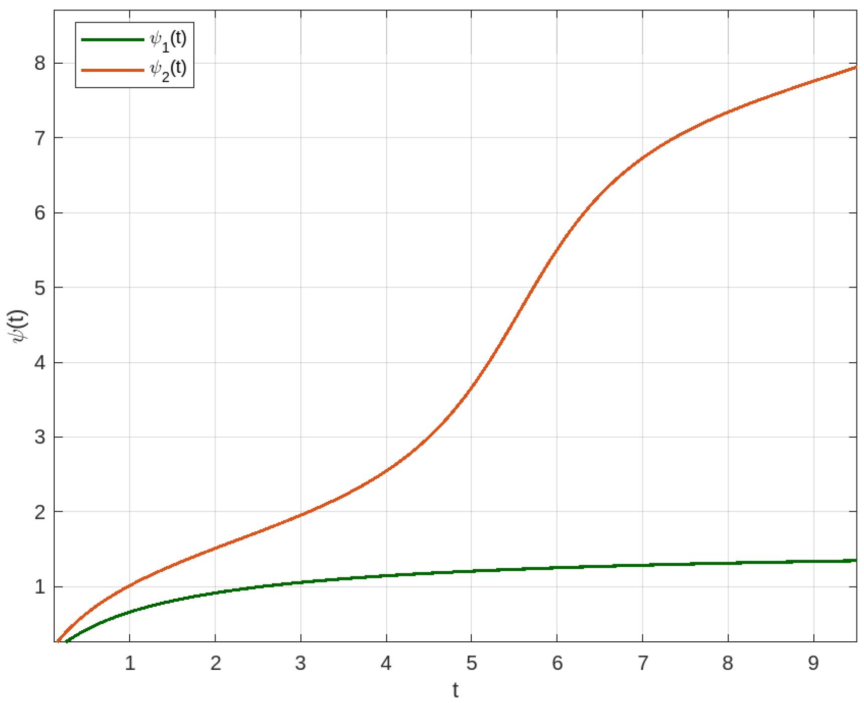
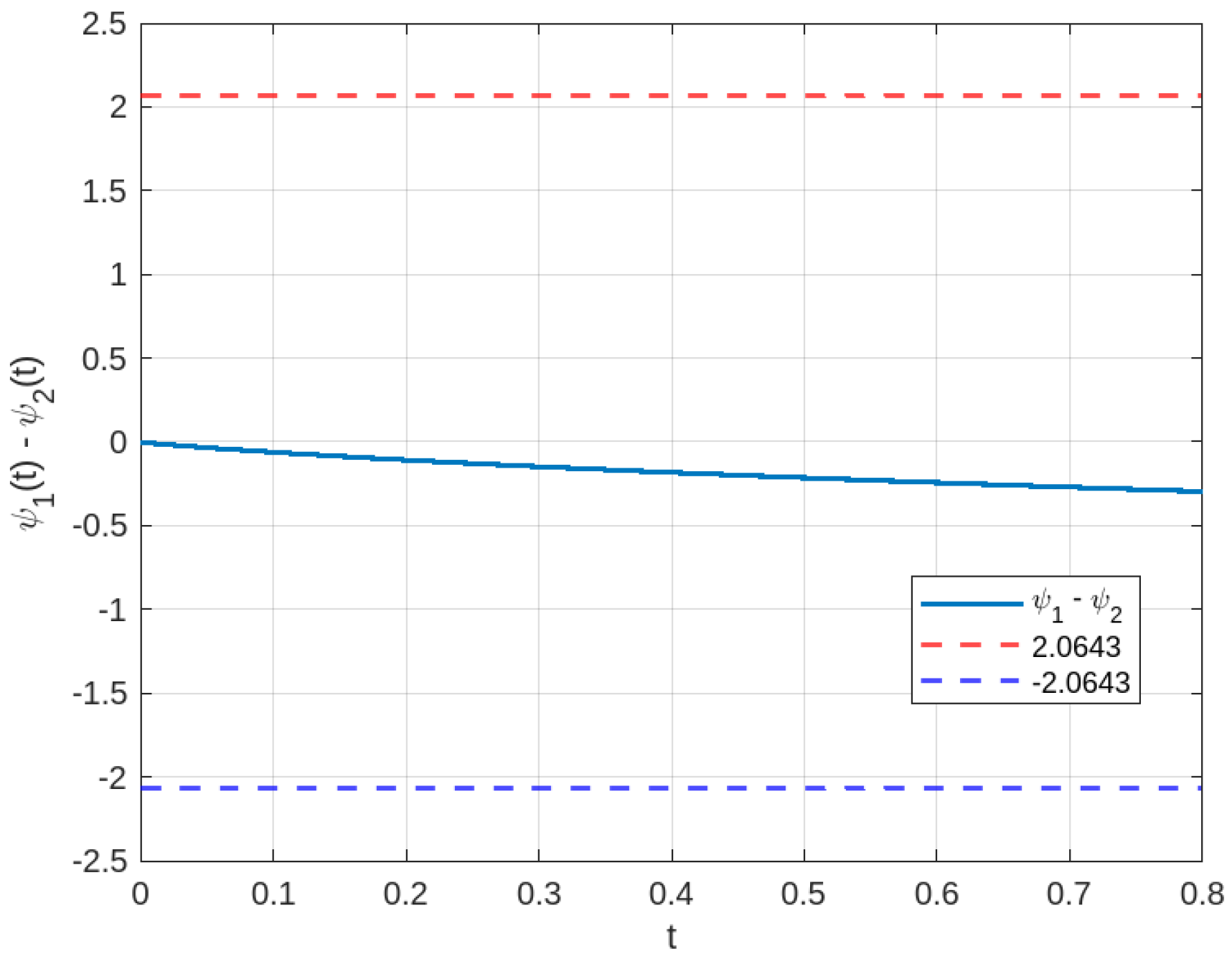
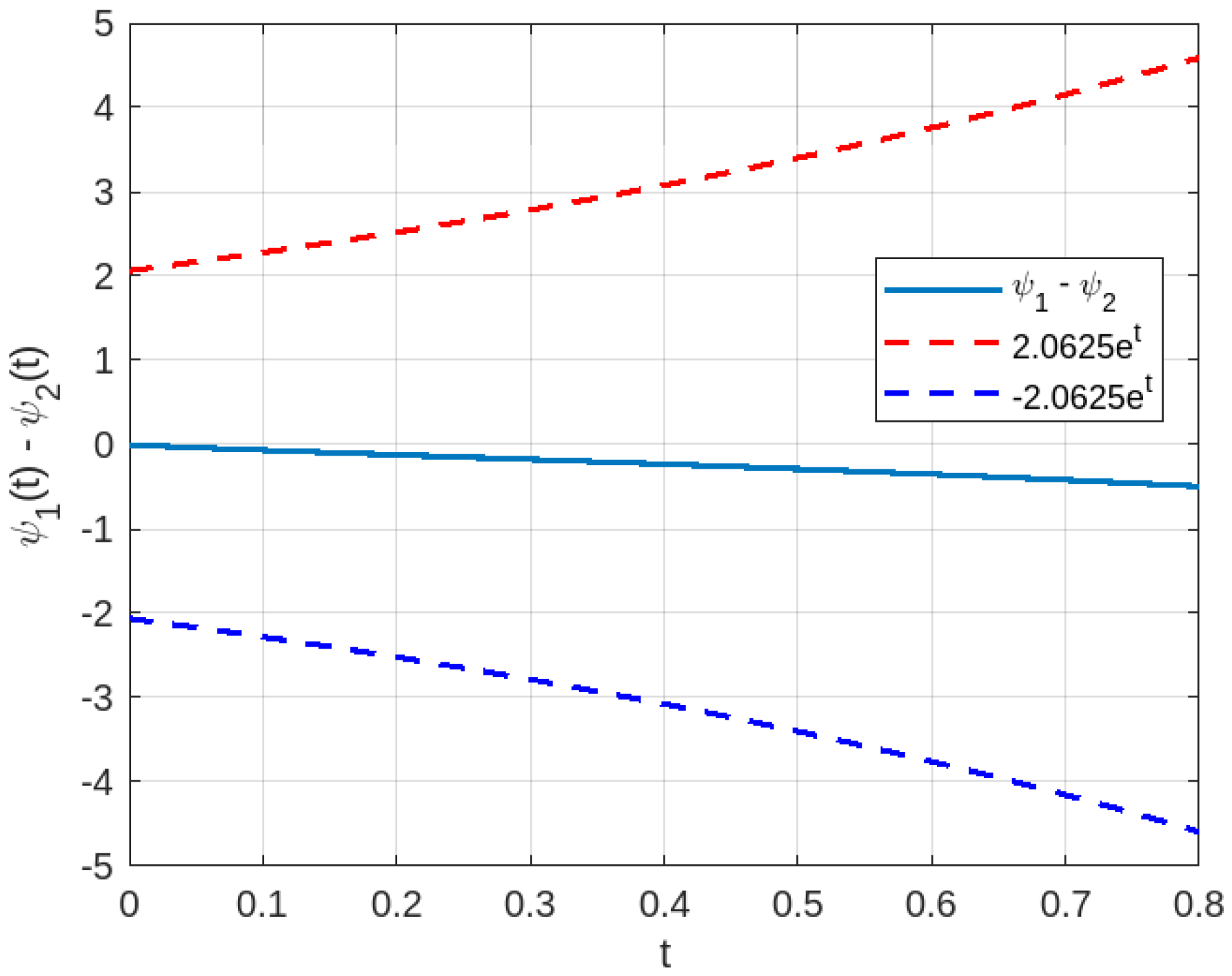
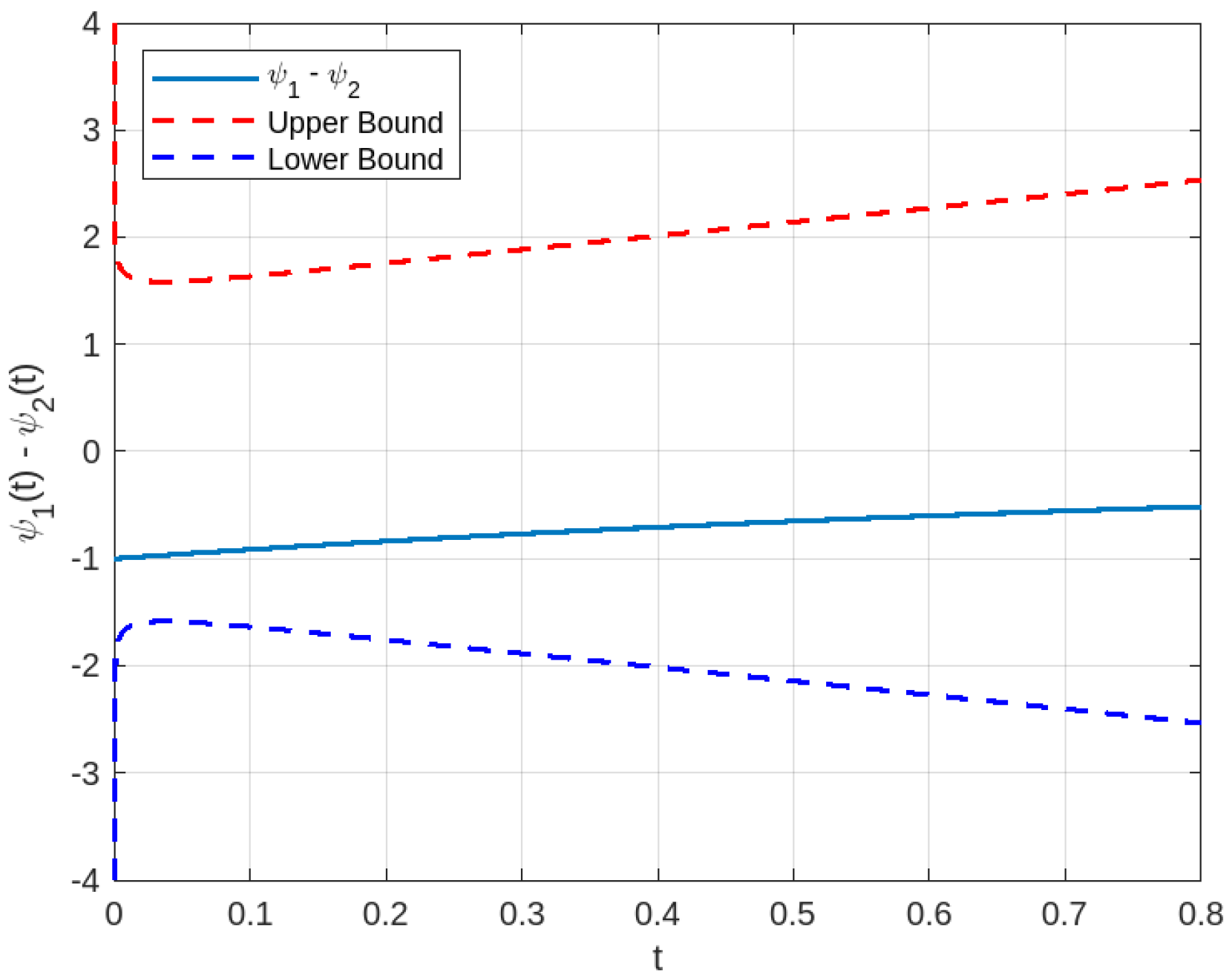
For the numerical simulations in Example 3, we employed the Adams–Bashforth–Moulton method in MATLAB R2025a to generate solution graphs and validate our theoretical results. This method was chosen for its optimal balance between computational efficiency and accuracy in solving implicit fractional differential equations.

In this study, we generalize Gronwall’s inequality as a key tool for analyzing stability and continuous dependence in constant-order fractional differential equations. Furthermore, we demonstrate the potential to extend this work to variable-order fractional problems by developing a generalized Gronwall-type inequality for variable-order fractional derivatives.

9. Conclusions

This work advances the analysis of nonlinear implicit Hilfer fractional differential equations of general order in weighted spaces by establishing a unified framework for existence, uniqueness, and stability results. Through the combined application of Schaefer’s fixed-point theorem and Banach’s contraction principle, we have demonstrated the solvability of Cauchy-type problems under explicit hypotheses. The development of a generalized Gronwall inequality with singular kernels has further enabled rigorous investigation of Ulam-type stability, including Ulam–Hyers, Ulam–Hyers–Rassias, and their generalized variants, while also establishing continuous dependence on initial data.

Our results significantly expand the theoretical foundation for fractional differential equations with implicit structure, particularly in the weighted function spaces where such systems naturally occur. The developed methodology and stability criteria offer potential applications in modeling anomalous transport phenomena and memory-dependent processes. Future research directions may include extensions to variable-order systems and the incorporation of stochastic perturbations.