Analysis of Stability of Delayed Quaternion-Valued Switching Neural Networks via Symmetric Matrices

Abstract

The stability of a class of quaternion-valued switching neural networks (QVSNNs) with time-varying delays is investigated in this paper. Limited prior research exists on the stability analysis of quaternion-valued neural networks (QVNNs). This paper addresses the stability analysis of quaternion-valued neural networks (QVNNs). With the help of some symmetric matrices with excellent properties, the stability analysis method in this paper is undecomposed. The QVSNN discussed herein evolves with average dwell time. Based on the Lyapunov theoretical framework and Wirtinger-based inequality, QVSNNs under any switching law have global asymptotic stability (GAS) and global exponential stability (GES). The state decay estimation of the system is also given and proved. Finally, the effective and practical applicability of the proposed method is demonstrated by two comprehensive numerical calculations.

1. Introduction

Quaternions are the expanded form of real and complex numbers, comprising a real component paired with three orthogonal imaginary components. With the advancement of deep learning, researchers have begun to explore the possibility of incorporating quaternions into neural networks (NNs). Early studies primarily focused on the mathematical properties of quaternions. In recent years, QVNNs have demonstrated promising applications in areas such as satellite attitude control (UAV attitude control and multi-degree-of-freedom vehicle control) [1,2,3] and robotic motion control (robotic arm end-effector trajectory tracking, humanoid robot gait planning, and vibration suppression in flexible robotic arms) [4,5]. Researchers have proposed quaternion-valued convolutional NNs for processing color images and video data [6,7,8]. Quaternion-valued recurrent NNs have been utilized for processing time series data and natural language processing tasks [9,10]. These applications are closely related to the dynamic characteristics of QVNNs. Therefore, analyzing the stability of QVNNs is both necessary and meaningful. Essentially, it utilizes its high-dimensional algebraic structure, parameter efficiency, and physical interpretability to achieve more robust learning dynamics in complex tasks. This brings unique advantages in terms of higher-dimensional feature representation and stability, parameter efficiency and generalization ability, and robustness to complex perturbations and facilitates the long-term stability of dynamic systems. Recently, Wang [11], Humphries [12], Yang [13], and Shu [14] used the method of decomposing quaternions to analyze the stability of QVNNs. However, using decomposition to handle quaternions increases the computational complexity of the model, which means that a quaternion has to be decomposed into four real numbers to be computed. It also increases the conservatism of the activation function, which is demonstrated by the fact that the real and imaginary parts of the activation function can be separated, whereas in practice, it is possible that a quaternion -valued function does not fulfill this condition. If the undecomposed method is used, then the multiplication of quaternions (conjugate, dot product, etc.) can be accomplished by 16 real multiplications and additions, reducing the number of computational steps, and the overall operation is consistent with properties such as multiplicative combinativity. Therefore, for this study, the direct quaternion approach was used to reduce the computational cost and ensure a wider range of applicability for the system proposed in this paper.

In the modeling and design of NNs, time-varying delays are frequently encountered due to delays in information processing, which is also a source of oscillations in neural systems. Therefore, it is both necessary and meaningful to consider time-varying delays in the process of stability analysis for NNs. In recent years, Chen [15] discussed leakage delays and discrete delays. Song [16] addressed neutral-type delays. You [17] explored mixed time-varying delays. Wu [18], Shen [19], and Liu [20] discussed state delays. Tu [21] discussed discrete and distributed delays. Although many researchers have considered time-varying delays during stability analysis, fewer have considered both state time-varying delays and neutral-type time-varying delays. Therefore, in this paper, both state time-varying delays and neutral-type time-varying delays are taken into account simultaneously, helping to expand the applicability of the model and more accurately characterize the dynamic behavior of NNs.

A switching system is composed of multiple dynamic modes and a switching rule. Given a switching rule, a mode will be activated at a specific time and evolve over time intervals. System switching approaches are generally categorized into two types: time-dependent switching [22] and mode-dependent switching [23]. Time-dependent switching is based on switching at fixed time intervals, and state-dependent switching is based on switching when the system state reaches a specified switching threshold. This means that state-dependent switching is more complex than time-dependent switching, so time-dependent switching is used to reduce the complexity in this paper. Switching neural networks(SNNs) are a specialized form of NNs that incorporate the concept of switching. Such systems are capable of switching among multiple NNs subsystems in accordance with shifting external conditions and operational needs, thereby achieving more flexible and efficient information processing and control. Applications of such systems encompass associative memory and knowledge representation [24], control systems and automation [25], pattern recognition and image processing [26,27], and other related research areas. These wide-ranging applications are inextricably linked to the stability of SNNs. Bao [28] discussed the resilient fixed-time stability of SNNs affected by impulsive deception attacks; a novel theorem for the fixed-time stability of impulsive systems was established by virtue of the comparison principle. Guo [29] discussed the multistability of SNNs under state-dependent switching; the switching threshold was found to play an important role in stabilizing the equilibrium in the unsaturated region of the activation function. Jiao [30] discussed the stability of stochastic impulsive and SNNs; a result concerned with the existence and uniqueness of solutions to random impulsive and switching neural networks was developed under some general conditions. Yang [31] discussed the robust stability of stochastic SNNs, and Wu [32] discussed the GES of NNs with switching parameters, combining the mean residence time method with the segmented Lyapunov function technique. The above studies discussed a certain stability of the SNNs, while fewer studies discuss different stabilities at the same time. Therefore, we discuss both GAS (the state eventually converges to the equilibrium point, but the convergence speed is not explicitly specified) and GES (the state converges to the equilibrium point at an exponential rate, and the convergence rate is clear and fast) of SNNs and give more comprehensive stability results in this paper.

From the above discussion, we know that most of the current studies on quaternion-valued neural networks [11,12,13,14] do not consider switching, and the studies on switching neural networks [28,30,31,32] do not consider quaternions. Therefore, we try to combine quaternion and switching neural networks and use the method of undecomposition to deal with the quaternion while considering state time-varying time delay and neutral-type time-varying time delay. The research method is relatively novel and has some research significance. Meanwhile, the QVSNN model is not only limited to the theoretical establishment but is also necessary in practice. It has a wide range of practical applications in 3D/4D motion analysis, weather forecasting, electromagnetic signal processing, image matching, EEG/EMI signal analysis, medical image fusion, and UAV swarm collaboration.

Based on existing discussions, this paper endeavors to establish sufficient conditions for the GAS and GES of a class of QVSNNs with state time-varying delays and neutral-type time-varying delays. Our key contributions are summarized below:

(1)

The combination of quaternions and switching neural networks has been rarely studied, so in this paper, we try to explore the stability of QVSNNs by analysing the properties of some symmetric matrices in an undecomposed approach.

(2)

The QVSNN discussed in this paper has a global asymptotic stability under arbitrary switching laws and a global exponential stability under a given switching sequence and switching condition;

(3)

The Wirtinger-based inequality is generalized to the domain of quaternions and used in the analysis of stability, where the method of proof differs from the existing literature.

The remainder of this paper is structured as follows: Section 2 introduces the studied system and formulates the underlying assumptions, formal definitions, and core lemmas. In Section 3, two key theorems are given, and their accuracy is proved by means of rigorous theoretical derivations. Section 4 verifies the theoretical analysis through numerical simulations. Finally, Section 5 gives conclusions.

2. Preliminaries

Notations: Let $\mathfrak{R}$ (reals), $\mathfrak{C}$ (complexes), and $\mathfrak{Q}$ (quaternions) denote the respective number systems. The matrix spaces ${\mathfrak{R}}^{n\times n}$, ${\mathfrak{C}}^{n\times n}$, and ${\mathfrak{Q}}^{n\times n}$ consist of all $n\times n$ matrices over $\mathfrak{R}$, $\mathfrak{C}$, and $\mathfrak{Q}$, correspondingly. We write ${\mathfrak{R}}^n$ (resp. ${\mathfrak{C}}^n$, ${\mathfrak{Q}}^n$) for the space of n-dimensional real (resp. complex, quaternion) vectors. Let ${\mathcal{A}}^T$ be the transpose, $\overline{\mathcal{A}}$ the conjugate, and ${\mathcal{A}}^{*}$ = ${\overline{\mathcal{A}}}^T$ the conjugate transpose of matrix $\mathcal{A}$. For any ${\mathcal{A}\in \mathfrak{Q}}^{n\times n}$, the module of $\mathcal{A}$ is denoted by $\left|\mathcal{A}\right|$, while $\Vert \mathcal{A}\Vert$ indicates its norm, and ${\lambda }_{min}\left(\mathcal{A}\right)$ and ${\lambda }_{max}\left(\mathcal{A}\right)$ correspond to the minimum and maximum eigenvalues, respectively.

2.1. Quaternion Algebra

Quaternions are an associative algebra defined over the real field $\mathfrak{R}$. The real form of a quaternion can be expressed as follows:

$$\mathcal{U}={\mathcal{U}}_0+{\mathcal{U}}_1{\xi }_1+{\mathcal{U}}_2{\xi }_2+{\mathcal{U}}_3{\xi }_3\in \mathfrak{Q}.$$

with a real component $\mathfrak{R}\left(\mathcal{U}\right)={\mathcal{U}}_0$ and a vector component $\mathfrak{I}\left(\mathcal{U}\right)={\mathcal{U}}_1{\xi }_1+{\mathcal{U}}_2{\xi }_2+{\mathcal{U}}_3{\xi }_3$, where ${\mathcal{U}}_0,{\mathcal{U}}_1,{\mathcal{U}}_2,{\mathcal{U}}_3$ are real coefficients. The basis elements ${\xi }_1,{\xi }_2,{\xi }_3$ satisfy the following relations:

$${\xi }_1^2={\xi }_2^2={\xi }_3^2=-1,{\xi }_1{\xi }_2=-{\xi }_2{\xi }_1={\xi }_3,{\xi }_2{\xi }_3=-{\xi }_3{\xi }_2={\xi }_1,{\xi }_3{\xi }_1=-{\xi }_1{\xi }_3={\xi }_2.$$

This defines a non-commutative multiplication operation in the quaternion algebra.

For any two quaternions $\mathcal{V}={\mathcal{V}}_0+{\mathcal{V}}_1{\xi }_1+{\mathcal{V}}_2{\xi }_2+{\mathcal{V}}_3{\xi }_3$ and $\mathcal{U}={\mathcal{U}}_0+{\mathcal{U}}_1{\xi }_1+{\mathcal{U}}_2{\xi }_2+{\mathcal{U}}_3{\xi }_3$, give the operation between them.

(i)

Additive operation:

$$\begin{array}{c}\hfill \mathcal{V}+\mathcal{U}=\left({\mathcal{V}}_0+{\mathcal{U}}_0\right)+\left({\mathcal{V}}_1+{\mathcal{U}}_1\right){\xi }_1+\left({\mathcal{V}}_2+{\mathcal{U}}_2\right){\xi }_2+\left({\mathcal{V}}_3+{\mathcal{U}}_3\right){\xi }_3;\end{array}$$

(ii)

Multiplication operation:

$$\begin{array}{cc}\hfill \mathcal{V}\mathcal{U}& =\left({\mathcal{V}}_0{\mathcal{U}}_0-{\mathcal{V}}_1{\mathcal{U}}_1-{\mathcal{V}}_2{\mathcal{U}}_2-{\mathcal{V}}_3{\mathcal{U}}_3\right)\hfill \\ \hfill & +\left({\mathcal{V}}_0{\mathcal{U}}_1+{\mathcal{V}}_1{\mathcal{U}}_0+{\mathcal{V}}_2{\mathcal{U}}_3-{\mathcal{V}}_3{\mathcal{U}}_2\right){\xi }_1\hfill \\ \hfill & +\left({\mathcal{V}}_0{\mathcal{U}}_2+{\mathcal{V}}_2{\mathcal{U}}_0-{\mathcal{V}}_1{\mathcal{U}}_3+{\mathcal{V}}_3{\mathcal{U}}_1\right){\xi }_2\hfill \\ & +\left({\mathcal{V}}_0{\mathcal{U}}_3+{\mathcal{V}}_3{\mathcal{U}}_0+{\mathcal{V}}_1{\mathcal{U}}_2-{\mathcal{U}}_2{\mathcal{V}}_1\right){\xi }_3.\hfill \end{array}$$

For a given quaternion $\mathcal{U}={\mathcal{U}}_0+{\mathcal{U}}_1{\xi }_1+{\mathcal{U}}_2{\xi }_2+{\mathcal{U}}_3\xi$, we denote the conjugate of $\mathcal{U}$ by $\overline{\mathcal{U}}$.

$$\overline{\mathcal{U}}={\mathcal{U}}_0-{\mathcal{U}}_1{\xi }_1-{\mathcal{U}}_2{\xi }_2-{\mathcal{U}}_3{\xi }_3.$$

The definitions of the modulus of $\mathcal{U}$ are given below:

$$\begin{array}{c}\hfill \left|\mathcal{U}\right|=\sqrt{\mathcal{U}{\mathcal{U}}^{*}}=\sqrt{{\mathcal{U}}_0^2+{\mathcal{U}}_1^2+{\mathcal{U}}_2^2+{\mathcal{U}}_3^2.}\end{array}$$

For a given vector $\mathcal{U}=({\mathcal{U}}_1,\dots ,{\mathcal{U}}_n)\in {\mathfrak{Q}}^n$, the definitions of the norm of $\mathcal{U}$ are given below:

$$\Vert \mathcal{U}\Vert =\sqrt{\sum _{i=1}^n{\left|{\mathcal{U}}_i\right|}^2}.$$

2.2. Model Description

In general, we represent a switching system that switches according to time(s) by the following differential equation:

$$\dot{\mathcal{Ƶ}}\left(s\right)=g_{△\left(s\right)}\left(s,\mathcal{Ƶ}\left(s\right)\right),$$

(1)

where $△\left(s\right)$ is the switching signal, and it is a right-continuous segmented constant-valued function $△\left(s\right):\left[0\right.,\left.\infty \right)\to \mathbb{Z}=\left\{1,2,\dots ,n\right\}$, where $\mathbb{Z}$ is the subsystem index set. $△\left(s\right)=\mathcal{B},\mathcal{B}\in \mathbb{Z}$ denotes that the $\mathcal{B}$th subsystem is activated.

This study examines the dynamical behaviour of QVSNNs with time-varying delays under the action of switching signals, whose models are described as follows:

$$\begin{array}{ccc}\hfill g_{△\left(s\right)}\left(s,\mathcal{Ƶ}\left(s\right)\right)& =& -A_{△\left(S\right)}\mathcal{Ƶ}\left(s\right)+B_{△\left(s\right)}f\left(\mathcal{Ƶ}\left(s\right)\right)+C_{△\left(s\right)}f\left(\mathcal{Ƶ}\left(s-\delta \left(s\right)\right)\right)\hfill \\ & & +D_{△\left(t\right)}\dot{\mathcal{Ƶ}}\left(s-\varrho \left(s\right)\right)+\Xi ,\hfill \end{array}$$

(2)

where $\mathcal{Ƶ}\left(s\right)={\left({\mathcal{Ƶ}}_1\left(s\right),{\mathcal{Ƶ}}_2\left(s\right),\dots ,{\mathcal{Ƶ}}_n\left(s\right)\right)}^T\in {\mathfrak{Q}}^n$ is the state vector of the neuron, $f\left(·\right)=\left(f_1\left(·\right),f_2\left(·\right),\dots ,\right.{\left.f_n\left(·\right)\right)}^T\in {\mathfrak{Q}}^n$ is the activation function of the neuron, $A_{△\left(s\right)}\in {\mathfrak{R}}^{n\times n}$ is a positive definite diagonal matrix, $B_{△\left(s\right)}={\left(b_{ij}\right)}_{n\times n}$, $C_{△\left(s\right)}={\left(c_{ij}\right)}_{n\times n}$, and $D_{△\left(s\right)}={\left(d_{ij}\right)}_{n\times n}\in {\mathfrak{Q}}^{n\times n}$ are the matrix of connection rights. $\Xi ={\left({\Xi }_1,{\Xi }_2,\dots {\Xi }_n\right)}^T\in {\mathfrak{Q}}^n$ is an external input to a neural network, $\delta \left(s\right)$ is state time delays, and $\varrho \left(s\right)$ is neutral-type time delays.

To make it easier to analyze, we transform (2) into the following model (3) for the equilibrium point at the origin, and subsequent studies are based on this model, described as follows:

$$\left\{\begin{array}{c}\dot{\mathcal{Ƶ}}\left(s\right)=-A_{△\left(s\right)}\mathcal{Ƶ}\left(s\right)+B_{△\left(s\right)}f\left(\mathcal{Ƶ}\left(s\right)\right)+C_{△\left(s\right)}f\left(\mathcal{Ƶ}\left(s-\delta \left(s\right)\right)\right)+D_{△\left(s\right)}\dot{\mathcal{Ƶ}}\left(s-\varrho \left(s\right)\right),\hfill \\ \mathcal{Ƶ}\left(s\right)=ð\left(s\right),ð\left(s\right)\in \left[-{\delta }_M,0\right],\hfill \end{array}\right.$$

(3)

the parameters in model (3) are consistent with those in model (2), and $ð\left(t\right)$ is the initial value of the neuron state.

A schematic of the quaternion -valued switching neural network model (3) is given below in Figure 1.

The structural framework of QVSNN can be clearly seen from the above diagram, where switching between n subsystems is performed, and the switching signals only need to satisfy the given switching sequences and average dwell time.

Some assumptions needed for this paper are given below.

Assumption 1.

The activation function $f\left(s\right)$ is a bounded function and satisfies $f\left(0\right)=0$.

Assumption 2.

Diagonal matrices such as $\mathcal{L}=diag\left({\mathcal{L}}_1,{\mathcal{L}}_2,\dots ,{\mathcal{L}}_n\right)>0\in {\mathfrak{R}}^n$ exist, meaning that

$$\left|f_i\left({\mathfrak{U}}_1\right)-f_i\left({\mathfrak{U}}_2\right)\right|\le {\mathcal{L}}_i\left|{\mathfrak{U}}_1-{\mathfrak{U}}_2\right|,\forall {\mathfrak{U}}_1,{\mathfrak{U}}_2\in \mathfrak{Q},{\mathcal{L}}_i\in \mathfrak{R},i=1,2,\dots ,n.$$

Assumption 3.

For $\delta \left(s\right)$ and $\varrho \left(s\right)$, $\forall s\ge 0$ and constant ${\delta }_m\ge 0,{\delta }_M\ge 0,{\varrho }_m\ge 0,{\varrho }_M\ge 0,$$\delta >0,\varrho >0$ satisfies

$$\begin{array}{cc}\hfill & 0\le {\delta }_m\le \delta \left(s\right)\le {\delta }_M,\dot{\delta }\left(s\right)\le \delta <1,\hfill \\ & 0\le {\varrho }_m\le \varrho \left(s\right)\le {\varrho }_M,\dot{\varrho }\left(s\right)\le \varrho <1.\hfill \end{array}$$

We give the above assumptions due to the fact that bounded activation functions are advantageous in scenarios that require stable outputs (e.g., control tasks, financial forecasting). In control systems where inference or training of neural networks must be completed in a fixed time (e.g., robot control), delay bounds ensure that the system response time satisfies the stability condition. Overall, assumptions such as bounded activation functions and delay bounds are not purely mathematical abstractions, but rather a bridge between theoretical stability and engineering practice. Although practical systems may not fully satisfy these ideal conditions, they provide a framework for designing robust, interpretable neural networks and have spawned numerous practical techniques (e.g., gradient tailoring, delay compensation).

Assumption 4.

For $△\left(s\right)$, the following switching sequence is designed:

$$△\left(s\right)=\left\{\left({\mathcal{B}}_0,s_0\right),\left({\mathcal{B}}_1,s_1\right),\dots ,\left({\mathcal{B}}_m,s_m\right),\dots |{\mathcal{B}}_m\in \mathbb{Z},m=0,1,\dots ,n\right\},$$

where $0=s_0<s_1<s_2<\dots <s_m<\dots$, and the ${\mathcal{B}}_m$th subsystem is activated when $s\in \left[s_m,\right.\left.s_{m+1}\right)$.

The definitions and lemmas needed for this paper are given below.

Definition 1.

If there is constant $\eta >0$ and $\gamma >0$ such that

$$∥\mathcal{Ƶ}\left(s\right)∥\le \eta ∥\mathcal{Ƶ}\left(s_0\right)∥e^{-\gamma \left(s-s_0\right)},\forall s\ge s_0,$$

then system (3) is GES.

Definition 2.

If there exists ${\mathbb{Z}}_0\ge 0,\mathbb{Z}=\left\{1,2,\dots ,n\right\},\forall S_1\le S_2$ such that

$$\begin{array}{c}\hfill {\mathbb{Z}}_{\sigma }\left(S_1,S_2\right)\le {\mathbb{Z}}_0+{\displaystyle \frac{S_2-S_1}{S_a}},\end{array}$$

where ${\mathbb{Z}}_{\sigma }\left(S_1,S_2\right)$ count the switchings of $△\left(s\right)$ on $\left(S_1,S_2\right)$, $S_a$ represents the average dwell time, and ${\mathbb{Z}}_0$ is the chatter bound; for computational simplicity, we set ${\mathbb{Z}}_0=0$.

Lemma 1.

[15] Given a positive definite matrix $K\in {\mathfrak{Q}}^{n\times n}$ (Hermitian) and a function $\vartheta \left(\kappa \right):\left[a,b\right]\to {\mathfrak{Q}}^n$ ($a<b$), the following inequality holds:

$${\left({\int }_a^b\vartheta \left(\kappa \right)d\kappa \right)}^{*}K\left({\int }_a^b\vartheta \left(\kappa \right)d\kappa \right)\le \left(b-a\right){\int }_a^b{\vartheta }^{*}\left(\kappa \right)K\vartheta \left(\kappa \right)d\kappa .$$

Lemma 2.

[33] Given a matrix $\mathsf{\Gamma }=\mathsf{\Gamma }{\xi }_0+\mathsf{\Gamma }{\xi }_1+\mathsf{\Gamma }{\xi }_2+\mathsf{\Gamma }{\xi }_3\in {\mathfrak{Q}}^{n\times n}$ (Hermitian), then $\mathsf{\Gamma }<0$ is equivalent to

$$\begin{array}{c}\hfill \left[\begin{array}{cc}\begin{array}{cc}\mathsf{\Gamma }{\xi }_0& -\mathsf{\Gamma }{\xi }_2\\ \mathsf{\Gamma }{\xi }_2& \mathsf{\Gamma }{\xi }_0\end{array}& \begin{array}{cc}-\mathsf{\Gamma }{\xi }_1& \mathsf{\Gamma }{\xi }_3\\ \mathsf{\Gamma }{\xi }_3& \mathsf{\Gamma }{\xi }_1\end{array}\\ \begin{array}{cc}\mathsf{\Gamma }{\xi }_1& -\mathsf{\Gamma }{\xi }_3\\ -\mathsf{\Gamma }{\xi }_3& -\mathsf{\Gamma }{\xi }_1\end{array}& \begin{array}{cc}\mathsf{\Gamma }{\xi }_0& -\mathsf{\Gamma }{\xi }_2\\ \mathsf{\Gamma }{\xi }_2& \mathsf{\Gamma }{\xi }_0\end{array}\end{array}\right]<0.\end{array}$$

Lemma 3.

(Wirtinger-based inequality) For any positive definite matrix $\mathcal{H}\in {\mathfrak{Q}}^{n\times n}$ (Hermitian), the function $\zeta \left(\kappa \right):\left[c,d\right]\to {\mathfrak{Q}}^n$ is continuously differentiable, and the following inequality holds:

$$\begin{array}{c}\hfill {\int }_c^d{\dot{\zeta }}^{*}\left(\kappa \right)\mathcal{H}\dot{\zeta }\left(\kappa \right)d\kappa \ge {\displaystyle \frac{1}{d-c}}{\left(\zeta \left(d\right)-\zeta \left(c\right)\right)}^{*}\mathcal{H}\left(\zeta \left(d\right)-\zeta \left(c\right)\right)+{\displaystyle \frac{3}{d-c}}{\aleph }^{*}\mathcal{H}\aleph ,\end{array}$$

where

$$\aleph =\zeta \left(d\right)+\zeta \left(c\right)-{\displaystyle \frac{2}{d-c}}{\int }_c^d\zeta \left(\kappa \right)d\kappa .$$

Proof. 

By Lemma 2, we can find that $\mathcal{H}>0$ is equivalent to

$$\begin{array}{c}\hfill \left[\begin{array}{cc}\begin{array}{cc}\mathcal{H}{\xi }_0& -\mathcal{H}{\xi }_2\\ \mathcal{H}{\xi }_2& \mathcal{H}{\xi }_0\end{array}& \begin{array}{cc}-\mathcal{H}{\xi }_1& \mathcal{H}{\xi }_3\\ \mathcal{H}{\xi }_3& \mathcal{H}{\xi }_2\end{array}\\ \begin{array}{cc}\mathcal{H}{\xi }_1& -\mathcal{H}{\xi }_3\\ -\mathcal{H}{\xi }_3& -\mathcal{H}{\xi }_1\end{array}& \begin{array}{cc}\mathcal{H}{\xi }_0& -\mathcal{H}{\xi }_2\\ \mathcal{H}{\xi }_2& \mathcal{H}{\xi }_0\end{array}\end{array}\right]>0.\end{array}$$

Because of $\zeta \left(\kappa \right):\left[c,d\right]\to {\mathfrak{Q}}^n$, it is found that $\dot{\zeta }\left(\kappa \right)={\dot{\zeta }}_1\left(\kappa \right)+{\dot{\zeta }}_2\left(\kappa \right){\xi }_1+{\dot{\zeta }}_3\left(\kappa \right){{\xi }_2+\dot{\zeta }}_4\left(\kappa \right){\xi }_3$, and then the following equation holds:

$$\begin{array}{cc}\hfill & {\int }_c^d{\dot{\zeta }}^{*}\left(\kappa \right)\mathcal{H}\dot{\zeta }\left(\kappa \right)d\kappa \hfill \\ & ={\int }_c^d{\left(\begin{array}{c}\begin{array}{c}{\dot{\zeta }}_1\left(\kappa \right)\\ {\dot{\zeta }}_2\left(\kappa \right)\end{array}\\ \begin{array}{c}{\dot{\zeta }}_3\left(\kappa \right)\\ {\dot{\zeta }}_4\left(\kappa \right)\end{array}\end{array}\right)}^T\left[\begin{array}{cc}\begin{array}{cc}\mathcal{H}{\xi }_0& -\mathcal{H}{\xi }_2\\ \mathcal{H}{\xi }_2& \mathcal{H}{\xi }_0\end{array}& \begin{array}{cc}-\mathcal{H}{\xi }_1& \mathcal{H}{\xi }_3\\ \mathcal{H}{\xi }_3& \mathcal{H}{\xi }_2\end{array}\\ \begin{array}{cc}\mathcal{H}{\xi }_1& -\mathcal{H}{\xi }_3\\ -\mathcal{H}{\xi }_3& -\mathcal{H}{\xi }_1\end{array}& \begin{array}{cc}\mathcal{H}{\xi }_0& -\mathcal{H}{\xi }_2\\ \mathcal{H}{\xi }_2& \mathcal{H}{\xi }_0\end{array}\end{array}\right]\left(\begin{array}{c}\begin{array}{c}{\dot{\zeta }}_1\left(\kappa \right)\\ {\dot{\zeta }}_2\left(\kappa \right)\end{array}\\ \begin{array}{c}{\dot{\zeta }}_3\left(\kappa \right)\\ {\dot{\zeta }}_4\left(\kappa \right)\end{array}\end{array}\right)d\kappa \hfill \\ & \ge {\displaystyle \frac{1}{d-c}}{\left(\begin{array}{c}\begin{array}{c}{\zeta }_1\left(d\right)-{\zeta }_1\left(c\right)\\ {\zeta }_2\left(d\right)-{\zeta }_2\left(c\right)\end{array}\\ \begin{array}{c}{\zeta }_3\left(d\right)-{\zeta }_3\left(c\right)\\ {\zeta }_4\left(d\right)-{\zeta }_4\left(c\right)\end{array}\end{array}\right)}^T\left[\begin{array}{cc}\begin{array}{cc}\mathcal{H}{\xi }_0& -\mathcal{H}{\xi }_2\\ \mathcal{H}{\xi }_2& \mathcal{H}{\xi }_0\end{array}& \begin{array}{cc}-\mathcal{H}{\xi }_1& \mathcal{H}{\xi }_3\\ \mathcal{H}{\xi }_3& \mathcal{H}{\xi }_2\end{array}\\ \begin{array}{cc}\mathcal{H}{\xi }_1& -\mathcal{H}{\xi }_3\\ -\mathcal{H}{\xi }_3& -\mathcal{H}{\xi }_1\end{array}& \begin{array}{cc}\mathcal{H}{\xi }_0& -\mathcal{H}{\xi }_2\\ \mathcal{H}{\xi }_2& \mathcal{H}{\xi }_0\end{array}\end{array}\right]\left(\begin{array}{c}\begin{array}{c}{\zeta }_1\left(d\right)-{\zeta }_1\left(c\right)\\ {\zeta }_2\left(d\right)-{\zeta }_2\left(c\right)\end{array}\\ \begin{array}{c}{\zeta }_3\left(d\right)-{\zeta }_3\left(c\right)\\ {\zeta }_4\left(d\right)-{\zeta }_4\left(c\right)\end{array}\end{array}\right)\hfill \\ & +{\displaystyle \frac{3}{d-c}}{\left(\left(\begin{array}{c}\begin{array}{c}{\zeta }_1\left(d\right)+{\zeta }_1\left(c\right)\\ {\zeta }_2\left(d\right)+{\zeta }_2\left(c\right)\end{array}\\ \begin{array}{c}{\zeta }_3\left(d\right)-{\zeta }_3\left(c\right)\\ {\zeta }_4\left(d\right)-{\zeta }_4\left(c\right)\end{array}\end{array}\right)-{\displaystyle \frac{2}{d-c}}{\int }_c^d\left(\begin{array}{c}\begin{array}{c}{\zeta }_1\left(\kappa \right)\\ {\zeta }_2\left(\kappa \right)\end{array}\\ \begin{array}{c}{\zeta }_3\left(\kappa \right)\\ {\zeta }_4\left(\kappa \right)\end{array}\end{array}\right)d\kappa \right)}^T\hfill \\ & \times \left[\begin{array}{cc}\begin{array}{cc}\mathcal{H}{\xi }_0& -\mathcal{H}{\xi }_2\\ \mathcal{H}{\xi }_2& \mathcal{H}{\xi }_0\end{array}& \begin{array}{cc}-\mathcal{H}{\xi }_1& \mathcal{H}{\xi }_3\\ \mathcal{H}{\xi }_3& \mathcal{H}{\xi }_2\end{array}\\ \begin{array}{cc}\mathcal{H}{\xi }_1& -\mathcal{H}{\xi }_3\\ -\mathcal{H}{\xi }_3& -\mathcal{H}{\xi }_1\end{array}& \begin{array}{cc}\mathcal{H}{\xi }_0& -\mathcal{H}{\xi }_2\\ \mathcal{H}{\xi }_2& \mathcal{H}{\xi }_0\end{array}\end{array}\right]\left(\left(\begin{array}{c}\begin{array}{c}{\zeta }_1\left(d\right)+{\zeta }_1\left(c\right)\\ {\zeta }_2\left(d\right)+{\zeta }_2\left(c\right)\end{array}\\ \begin{array}{c}{\zeta }_3\left(d\right)+{\zeta }_3\left(c\right)\\ {\zeta }_4\left(d\right)+{\zeta }_4\left(c\right)\end{array}\end{array}\right)-{\displaystyle \frac{2}{d-c}}{\int }_c^d\left(\begin{array}{c}\begin{array}{c}{\zeta }_1\left(\kappa \right)\\ {\zeta }_2\left(\kappa \right)\end{array}\\ \begin{array}{c}{\zeta }_3\left(\kappa \right)\\ {\zeta }_4\left(\kappa \right)\end{array}\end{array}\right)d\kappa \right)\hfill \\ & ={\displaystyle \frac{1}{d-c}}{\left(\zeta \left(d\right)-\zeta \left(c\right)\right)}^{*}\mathcal{H}\left(\zeta \left(d\right)-\zeta \left(c\right)\right)+{\displaystyle \frac{3}{d-c}}{\aleph }^{*}\mathcal{H}\aleph .\hfill \end{array}$$

□

By decomposing quaternions into their four real components, this work extends the Wirtinger-based inequality to the quaternion domain, thereby completing the proof.

In the above proof of the generalization of Lemma 3, we use the decomposition method, this is because we want to generalize Lemma 3 to quaternionic domains, but there are existing results that use the undecomposed method, so we try to use the decomposition method to generalize it and verify that this method is also feasible. This does not contradict our subsequent derivation, and the treatment of the main model in this paper still uses the undecomposed method.

The above inequality can also be transformed into the following linear matrix inequality:

$$\begin{array}{c}\hfill {\int }_c^d{\dot{\zeta }}^{*}\left(\kappa \right)\mathcal{H}\dot{\zeta }\left(\kappa \right)d\kappa \ge {\displaystyle \frac{1}{d-c}}{\tilde{\aleph }}^{*}\widetilde{œ}\tilde{\aleph },\end{array}$$

where

$$\widetilde{œ}=\left[\begin{array}{ccc}4\mathcal{H}& 2\mathcal{H}& -6\mathcal{H}\\ 2{\mathcal{H}}^{*}& 4\mathcal{H}& -6\mathcal{H}\\ -6{\mathcal{H}}^{*}& -6{\mathcal{H}}^{*}& 12\mathcal{H}\end{array}\right],$$

$$\tilde{\aleph }={\left[\begin{array}{ccc}{\zeta }^{*}\left(d\right)& {\zeta }^{*}\left(c\right)& {\displaystyle \frac{1}{d-c}}\end{array}{\int }_c^d{\zeta }^{*}\left(\kappa \right)d\kappa \right]}^{*}.$$

Remark 1.

The inequalities used during the stability analysis of neural networks have a significant impact on the conditions for determining stability. This paper employs Wirtinger-based inequalities to handle the quadratic term integrals; compared to other inequalities used in the literature [34,35], the Wirtinger-based inequality can provide tighter lower bounds. Moreover, these Wirtinger-based inequalities are transformed into linear matrix inequalities, making them more tractable.

3. Main Results

In this section, based on the Lyapunov theoretical framework, we will give three detailed proof procedures—for the GAS of system (3) under arbitrary switching laws, for the GES of system (3) under a given switching sequence, and for the GES of system (3) under the average dwell time condition—and estimations of the state decay by means of the Wirtinger-based inequality and the LMI techniques.

3.1. Global Asymptotic Stability

The proof procedure for the GAS of system (3) under an arbitrary switching law is given below.

Theorem 1.

Under Assumptions 1–3, if there exist symmetric matrices $P>0,Q_1>0,Q_2>0,$$Q_3>0,Q_4>0$, and $R_1>0\in {\mathfrak{R}}^{n\times n}$, then we have any matrix $M_1,M_2$, and $M_3\in {\mathfrak{R}}^{n\times n}$, guaranteeing the feasibility of the following LMIs:

$$\begin{array}{c}\hfill \Omega =\left[\begin{array}{ccccccc}{\Omega }_{11}& {\Omega }_{12}& 0& {\Omega }_{14}& {\Omega }_{15}& {\Omega }_{16}& 0\\ *& {\Omega }_{22}& 0& {\Omega }_{24}& M_2{B}_{\mathcal{B}}& M_2{C}_{\mathcal{B}}& 0\\ *& *& {\Omega }_{33}& 0& 0& 0& 0\\ *& *& *& {\Omega }_{44}& M_3{B}_{\mathcal{B}}& M_3{C}_{\mathcal{B}}& 0\\ *& *& *& *& {\Omega }_{55}& 0& 0\\ *& *& *& *& *& {\Omega }_{66}& 0\\ *& *& *& *& *& *& {\Omega }_{77}\end{array}\right]<0,\end{array}$$

(4)

with

$$\begin{array}{cc}\hfill & {\Omega }_{11}=-{A_{\mathcal{B}}}^{*}P-P^{*}{A}_{\mathcal{B}}+Q_1+{{\mathcal{L}}_1}^{*}{R}_1{\mathcal{L}}_1-M_1{A}_{\mathcal{B}}-{A_{\mathcal{B}}}^{*}{M_1}^{*},\hfill \\ & {\Omega }_{12}=-M_1-{A_{\mathcal{B}}}^{*}{M_2}^{*},\hfill \\ & {\Omega }_{14}=P^{*}{D}_{\mathcal{B}}+M_1{D}_{\mathcal{B}}-{A_{\mathcal{B}}}^{*}{M_3}^{*},\hfill \\ & {\Omega }_{15}=P^{*}{B}_{\mathcal{B}}+M_1{B}_{\mathcal{B}},\hfill \\ & {\Omega }_{16}=P^{*}{C}_{\mathcal{B}}+M_1{C}_{\mathcal{B}},\hfill \\ & {\Omega }_{22}=Q_3-M_2-{M_2}^{*}+{\delta }_M{Q}_4,\hfill \\ & {\Omega }_{24}=M_2{D}_{\mathcal{B}}-{M_3}^{*},\hfill \\ & {\Omega }_{33}=-\left(1-\delta \right)Q_1,\hfill \\ & {\Omega }_{44}=-\left(1-\varrho \right)Q_3+M_3{D}_{\mathcal{B}}+{D_{\mathcal{B}}}^{*}{M_3}^{*},\hfill \\ & {\Omega }_{55}=Q_2-R_1,\hfill \\ & {\Omega }_{66}=-\left(1-\delta \right)Q_2,\hfill \\ & {\Omega }_{77}=-{\displaystyle \frac{1}{{\delta }_M}}{Q}_4,\hfill \end{array}$$

Then, system (3) is GAS under any switching law.

Proof. 

Our analysis is based on the construction of a Lyapunov–Krasovskii functional with the following form:

$$V_{△\left(s\right)}\left(\mathcal{Ƶ}\left(s\right)\right)=\sum _{i=1}^5{V}_{i△\left(s\right)}\left(\mathcal{Ƶ}\left(t\right)\right),$$

(5)

with

$$\begin{array}{cc}\hfill & V_{1△\left(s\right)}\left(\mathcal{Ƶ}\left(s\right)\right)={\mathcal{Ƶ}}^{*}\left(s\right)P\mathcal{Ƶ}\left(s\right),\hfill \\ & V_{2△\left(s\right)}\left(\mathcal{Ƶ}\left(s\right)\right)={\int }_{s-\delta \left(s\right)}^s{\mathcal{Ƶ}}^{*}\left(\kappa \right)Q_1\mathcal{Ƶ}\left(\kappa \right)d\kappa ,\hfill \\ & V_{3△\left(s\right)}\left(\mathcal{Ƶ}\left(s\right)\right)={\int }_{s-\delta \left(s\right)}^s{f}^{*}\left(\mathcal{Ƶ}\left(\kappa \right)\right)Q_{2}f\left(\mathcal{Ƶ}\left(\kappa \right)\right)d\kappa ,\hfill \\ & V_{4△\left(s\right)}\left(\mathcal{Ƶ}\left(s\right)\right)={\int }_{s-\varrho \left(s\right)}^s{\dot{\mathcal{Ƶ}}}^{*}\left(\kappa \right)Q_3\dot{\mathcal{Ƶ}}\left(\kappa \right)d\kappa ,\hfill \\ & V_{5△\left(s\right)}\left(\mathcal{Ƶ}\left(s\right)\right)={\int }_{-{\delta }_M}^0{\int }_{s+\theta }^s{\dot{\mathcal{Ƶ}}}^{*}\left(\kappa \right)Q_4\dot{\mathcal{Ƶ}}\left(\kappa \right)d\kappa d\theta .\hfill \end{array}$$

Based on Assumption 3 and Lemma 1, combined with the dynamical behavior of the $\mathcal{B}$th subsystem described in (3), a derivative operation on $V\left(\mathcal{Ƶ}\left(s\right)\right)$ leads to

$$\begin{array}{cc}\hfill {\dot{V}}_{1\mathcal{B}}\left(\mathcal{Ƶ}\left(s\right)\right)& ={\stackrel{Ż}{\mathcal{Ƶ}}}^{*}\left(s\right)P\mathcal{Ƶ}\left(s\right)+{\mathcal{Ƶ}}^{*}\left(s\right)P^{*}\dot{\mathcal{Ƶ}}\left(s\right)\hfill \\ \hfill & ={\left(-A_{\mathcal{B}}\mathcal{Ƶ}\left(s\right)+B_{\mathcal{B}}f\left(\mathcal{Ƶ}\left(s\right)\right)+C_{\mathcal{B}}f\left(\mathcal{Ƶ}\left(s-\delta \left(s\right)\right)\right)+D_{\mathcal{B}}\dot{\mathcal{Ƶ}}\left(s-\varrho \left(s\right)\right)\right)}^{*}P\mathcal{Ƶ}\left(s\right)\hfill \\ \hfill & +{\mathcal{Ƶ}}^{*}\left(s\right)P^{*}\left(-A_{\mathcal{B}}\mathcal{Ƶ}\left(s\right)+B_{\mathcal{B}}f\left(\mathcal{Ƶ}\left(s\right)\right)+C_{\mathcal{B}}f\left(\mathcal{Ƶ}\left(s-\delta \left(s\right)\right)\right)+D_{\mathcal{B}}\dot{\mathcal{Ƶ}}\left(s-\varrho \left(s\right)\right)\right)\hfill \\ \hfill & ={\mathcal{Ƶ}}^{*}\left(s\right)\left(-A_{\mathcal{B}}^{*}P\right)\mathcal{Ƶ}\left(s\right)+f^{*}\left(\mathcal{Ƶ}\left(s\right)\right)\left(B_{\mathcal{B}}^{*}P\right)\mathcal{Ƶ}\left(s\right)\hfill \\ \hfill & +f^{*}\left(\mathcal{Ƶ}\left(s-\delta \left(s\right)\right)\right)\left(C_{\mathcal{B}}^{*}P\right)\mathcal{Ƶ}\left(s\right)+{\dot{\mathcal{Ƶ}}}^{*}\left(s-\varrho \left(s\right)\right)\left(D_{\mathcal{B}}^{*}P\right)\mathcal{Ƶ}\left(s\right)\hfill \\ \hfill & +{\mathcal{Ƶ}}^{*}\left(s\right)\left(-P^{*}{A}_{\mathcal{B}}\right)\mathcal{Ƶ}\left(s\right)+{\mathcal{Ƶ}}^{*}\left(s\right)\left(P^{*}{B}_{\mathcal{B}}\right)f\left(\mathcal{Ƶ}\left(s\right)\right)\hfill \\ \hfill & +{\mathcal{Ƶ}}^{*}\left(s\right)\left(P^{*}{C}_{\mathcal{B}}\right)f\left(\mathcal{Ƶ}\left(s-\delta \left(s\right)\right)\right)+{\mathcal{Ƶ}}^{*}\left(s\right)\left(P^{*}{D}_{\mathcal{B}}\right)\dot{\mathcal{Ƶ}}\left(s-\varrho \left(s\right)\right),\hfill \end{array}$$

(6)

$$\begin{array}{cc}\hfill {\dot{V}}_{2\mathcal{B}}\left(\mathcal{Ƶ}\left(s\right)\right)& ={\mathcal{Ƶ}}^{*}\left(s\right)Q_1\mathcal{Ƶ}\left(s\right)-\left(1-\dot{\delta }\left(s\right)\right){\mathcal{Ƶ}}^{*}\left(s-\delta \left(s\right)\right)Q_1\mathcal{Ƶ}\left(s-\delta \left(s\right)\right)\hfill \\ \hfill & \le {\mathcal{Ƶ}}^{*}\left(s\right)Q_1\mathcal{Ƶ}\left(s\right)-\left(1-\delta \right){\mathcal{Ƶ}}^{*}\left(s-\delta \left(s\right)\right)Q_1\mathcal{Ƶ}\left(s-\delta \left(s\right)\right),\hfill \end{array}$$

(7)

$$\begin{array}{cc}\hfill {\dot{V}}_{3\mathcal{B}}\left(\mathcal{Ƶ}\left(s\right)\right)& =f^{*}\left(\mathcal{Ƶ}\left(s\right)\right)Q_{2}f\left(\mathcal{Ƶ}\left(s\right)\right)-\left(1-\dot{\delta }\left(s\right)\right)f^{*}\left(\mathcal{Ƶ}\left(s-\delta \left(s\right)\right)\right)Q_{2}f\left(\mathcal{Ƶ}\left(s-\delta \left(s\right)\right)\right)\hfill \\ \hfill & \le f^{*}\left(\mathcal{Ƶ}\left(s\right)\right)Q_{2}f\left(\mathcal{Ƶ}\left(s\right)\right)-\left(1-\delta \right)f^{*}\left(\mathcal{Ƶ}\left(s-\delta \left(s\right)\right)\right)Q_{2}f\left(\mathcal{Ƶ}\left(s-\delta \left(s\right)\right)\right),\hfill \end{array}$$

(8)

$$\begin{array}{cc}\hfill {\dot{V}}_{4\mathcal{B}}\left(\mathcal{Ƶ}\left(s\right)\right)& ={\dot{\mathcal{Ƶ}}}^{*}\left(s\right)Q_3\dot{\mathcal{Ƶ}}\left(s\right)-\left(1-\varrho \left(s\right)\right){\dot{\mathcal{Ƶ}}}^{*}\left(s-\varrho \left(s\right)\right)Q_3\dot{\mathcal{Ƶ}}\left(s-\varrho \left(s\right)\right)\hfill \\ \hfill & \le {\dot{\mathcal{Ƶ}}}^{*}\left(s\right)Q_3\dot{\mathcal{Ƶ}}\left(s\right)-\left(1-\varrho \right){\dot{\mathcal{Ƶ}}}^{*}\left(s-\varrho \left(s\right)\right)Q_3\dot{\mathcal{Ƶ}}\left(s-\varrho \left(s\right)\right),\hfill \end{array}$$

(9)

$$\begin{array}{cc}\hfill {\dot{V}}_{5\mathcal{B}}\left(\mathcal{Ƶ}\left(s\right)\right)& ={\int }_{-{\delta }_M}^0{\dot{\mathcal{Ƶ}}}^{*}\left(s\right)Q_4\dot{\mathcal{Ƶ}}\left(s\right)-{\dot{\mathcal{Ƶ}}}^{*}\left(s-\theta \right)Q_4\dot{\mathcal{Ƶ}}\left(s-\theta \right)d\theta \hfill \\ \hfill & ={\delta }_M{\dot{\mathcal{Ƶ}}}^{*}\left(s\right)Q_4\dot{\mathcal{Ƶ}}\left(s\right)-{\int }_{-{\delta }_M}^0{\dot{\mathcal{Ƶ}}}^{*}\left(s-\theta \right)Q_4\dot{\mathcal{Ƶ}}\left(s-\theta \right)d\theta \hfill \\ \hfill & ={\delta }_M{\dot{\mathcal{Ƶ}}}^{*}\left(s\right)Q_4\dot{\mathcal{Ƶ}}\left(s\right)-{\int }_{s-{\delta }_M}^s{\dot{q}}^{*}\left(\kappa \right)Q_4\dot{\mathcal{Ƶ}}\left(\kappa \right)d\kappa \hfill \\ \hfill & \le {\delta }_M{\dot{\mathcal{Ƶ}}}^{*}\left(s\right)Q_4\dot{\mathcal{Ƶ}}\left(s\right)-{\displaystyle \frac{1}{{\delta }_M}}{\left({\int }_{s-{\delta }_M}^s\dot{\mathcal{Ƶ}}\left(\kappa \right)d\kappa \right)}^{*}{Q}_4\left({\int }_{s-{\delta }_M}^s\dot{\mathcal{Ƶ}}\left(\kappa \right)d\kappa \right).\hfill \end{array}$$

(10)

Due to the non-commutative nature of quaternion multiplication, it does not satisfy ${\dot{V}}_{1\mathcal{B}}\left(\mathcal{Ƶ}\left(s\right)\right)=2{\dot{\mathcal{Ƶ}}}^{*}\left(s\right)P\mathcal{Ƶ}\left(s\right)$ in the derivation of ${\dot{V}}_{1\mathcal{B}}\left(\mathcal{Ƶ}\left(s\right)\right)$, and we need to pay attention to the way quaternions are treated here.

For any matrix $M_1,M_2,M_3$, the following equation holds:

$$\begin{array}{cc}\hfill 0& =\left[\begin{array}{ccc}{\mathcal{Ƶ}}^{*}\left(s\right)& {\dot{\mathcal{Ƶ}}}^{*}\left(s\right)& {\dot{\mathcal{Ƶ}}}^{*}\left(s-\varrho \left(s\right)\right)\end{array}\right]\left[\begin{array}{c}{M}_1\\ M_2\\ M_3\end{array}\right]\hfill \\ & \times \left(-\dot{\mathcal{Ƶ}}\left(s\right)-A_{\mathcal{B}}\mathcal{Ƶ}\left(s\right)+B_{\mathcal{B}}f\left(\mathcal{Ƶ}\left(s\right)\right)+C_{\mathcal{B}}f\left(\mathcal{Ƶ}\left(s-\delta \left(s\right)\right)\right)+D_{\mathcal{B}}\dot{\mathcal{Ƶ}}\left(s-\varrho \left(s\right)\right)\right)\hfill \\ & +{\left(-\dot{\mathcal{Ƶ}}\left(s\right)-A_{\mathcal{B}}\mathcal{Ƶ}\left(s\right)+B_{\mathcal{B}}f\left(\mathcal{Ƶ}\left(s\right)\right)+C_{\mathcal{B}}f\left(\mathcal{Ƶ}\left(s-\delta \left(s\right)\right)\right)+D_{\mathcal{B}}\dot{\mathcal{Ƶ}}\left(s-\varrho \left(s\right)\right)\right)}^{*}\hfill \\ & \times \left[\begin{array}{ccc}{M_1}^{*}& {M_2}^{*}& {M_3}^{*}\end{array}\right]\left[\begin{array}{c}\mathcal{Ƶ}\left(s\right)\\ \dot{\mathcal{Ƶ}}\left(s\right)\\ \dot{\mathcal{Ƶ}}\left(s-\varrho \left(s\right)\right)\end{array}\right].\hfill \end{array}$$

(11)

Under Assumption 2, there exists ${\mathcal{L}}_1>0$, which leads to the following inequality:

$$\begin{array}{c}\hfill {\mathcal{Ƶ}}^{*}\left(s\right)\left({{{\mathcal{L}}_1}^{*}R}_1{\mathcal{L}}_1\right)\mathcal{Ƶ}\left(s\right)-f^{*}\left(\mathcal{Ƶ}\left(s\right)\right)R_{1}f\left(\mathcal{Ƶ}\left(s\right)\right)\ge 0.\end{array}$$

(12)

By (5)–(12), one can get

$$\begin{array}{cc}\hfill {\dot{V}}_{\mathcal{B}}\left(\mathcal{Ƶ}\left(s\right)\right)& ={\dot{V}}_{1\mathcal{B}}\left(\mathcal{Ƶ}\left(s\right)\right)+{\dot{V}}_{2\mathcal{B}}\left(\mathcal{Ƶ}\left(s\right)\right)+{\dot{V}}_{3\mathcal{B}}\left(\mathcal{Ƶ}\left(s\right)\right)+{\dot{V}}_{4\mathcal{B}}\left(\mathcal{Ƶ}\left(s\right)\right)+{\dot{V}}_{5\mathcal{B}}\left(\mathcal{Ƶ}\left(s\right)\right)\hfill \\ \hfill & \le {\mathcal{Ƶ}}^{*}\left(s\right)\left(-A_{\mathcal{B}}^{*}P\right)\mathcal{Ƶ}\left(s\right)+f^{*}\left(\mathcal{Ƶ}\left(s\right)\right)\left(B_{\mathcal{B}}^{*}P\right)\mathcal{Ƶ}\left(s\right)+f^{*}\left(\mathcal{Ƶ}\left(s-\delta \left(s\right)\right)\right)\left(C_{\mathcal{B}}^{*}P\right)\mathcal{Ƶ}\left(s\right)\hfill \\ \hfill & +{\dot{\mathcal{Ƶ}}}^{*}\left(s-\varrho \left(s\right)\right)\left(D_{\mathcal{B}}^{*}P\right)\mathcal{Ƶ}\left(s\right)+{\mathcal{Ƶ}}^{*}\left(s\right)\left(-P^{*}{A}_{\mathcal{B}}\right)\mathcal{Ƶ}\left(s\right)+{\mathcal{Ƶ}}^{*}\left(s\right)\left(P^{*}{B}_{\mathcal{B}}\right)f\left(\mathcal{Ƶ}\left(s\right)\right)\hfill \\ \hfill & +{\mathcal{Ƶ}}^{*}\left(s\right)\left(P^{*}{C}_{\mathcal{B}}\right)f\left(\mathcal{Ƶ}\left(s-\delta \left(s\right)\right)\right)+{\mathcal{Ƶ}}^{*}\left(s\right)\left(P^{*}{D}_{\mathcal{B}}\right)\dot{\mathcal{Ƶ}}\left(s-\varrho \left(s\right)\right)+{\mathcal{Ƶ}}^{*}\left(s\right)Q_1\mathcal{Ƶ}\left(s\right)\hfill \\ \hfill & -\left(1-\delta \right){\mathcal{Ƶ}}^{*}\left(s-\delta \left(s\right)\right)Q_1\mathcal{Ƶ}\left(s-\delta \left(s\right)\right)+f^{*}\left(\mathcal{Ƶ}\left(s\right)\right)Q_{2}f\left(\mathcal{Ƶ}\left(s\right)\right)\hfill \\ \hfill & -\left(1-\delta \right)f^{*}\left(\mathcal{Ƶ}\left(s-\delta \left(s\right)\right)\right)Q_{2}f\left(\mathcal{Ƶ}\left(s-\delta \left(s\right)\right)\right)+{\dot{\mathcal{Ƶ}}}^{*}\left(s\right)Q_3\dot{\mathcal{Ƶ}}\left(s\right)\hfill \\ \hfill & -\left(1-\varrho \right){\dot{\mathcal{Ƶ}}}^{*}\left(s-\varrho \left(s\right)\right)Q_3\dot{\mathcal{Ƶ}}\left(s-\varrho \left(s\right)\right)+{\delta }_M{\dot{\mathcal{Ƶ}}}^{*}\left(s\right)Q_4\dot{\mathcal{Ƶ}}\left(s\right)\hfill \\ \hfill & -{\displaystyle \frac{1}{{\delta }_M}}{\left({\int }_{s-{\delta }_M}^s\dot{\mathcal{Ƶ}}\left(\kappa \right)d\kappa \right)}^{*}{Q}_4\left({\int }_{s-{\delta }_M}^s\dot{\mathcal{Ƶ}}\left(\kappa \right)d\kappa \right)\hfill \\ \hfill & +{\mathcal{Ƶ}}^{*}\left(s\right)\left({{{\mathcal{L}}_1}^{*}R}_1{\mathcal{L}}_1\right)\mathcal{Ƶ}\left(s\right)-f^{*}\left(\mathcal{Ƶ}\left(s\right)\right)R_{1}f\left(\mathcal{Ƶ}\left(s\right)\right)\hfill \\ \hfill & +\left[\begin{array}{ccc}{\mathcal{Ƶ}}^{*}\left(s\right)& {\dot{\mathcal{Ƶ}}}^{*}\left(s\right)& {\dot{\mathcal{Ƶ}}}^{*}\left(s-\varrho \left(s\right)\right)\end{array}\right]\left[\begin{array}{c}{M}_1\\ M_2\\ M_3\end{array}\right]\hfill \\ \hfill & \times \left(-\dot{\mathcal{Ƶ}}\left(s\right)-A_{\mathcal{B}}\mathcal{Ƶ}\left(s\right)+B_{\mathcal{B}}f\left(\mathcal{Ƶ}\left(s\right)\right)+C_{\mathcal{B}}f\left(\mathcal{Ƶ}\left(s-\delta \left(s\right)\right)\right)+D_{\mathcal{B}}\dot{\mathcal{Ƶ}}\left(s-\varrho \left(s\right)\right)\right)\hfill \\ \hfill & +{\left(-\dot{\mathcal{Ƶ}}\left(s\right)-A_{\mathcal{B}}\mathcal{Ƶ}\left(s\right)+B_{\mathcal{B}}f\left(\mathcal{Ƶ}\left(s\right)\right)+C_{\mathcal{B}}f\left(\mathcal{Ƶ}\left(s-\delta \left(s\right)\right)\right)+D_{\mathcal{B}}\dot{\mathcal{Ƶ}}\left(s-\varrho \left(s\right)\right)\right)}^{*}\hfill \\ \hfill & \times \left[\begin{array}{ccc}{M_1}^{*}& {M_2}^{*}& {M_3}^{*}\end{array}\right]\left[\begin{array}{c}\mathcal{Ƶ}\left(s\right)\\ \dot{\mathcal{Ƶ}}\left(s\right)\\ \dot{\mathcal{Ƶ}}\left(s-\varrho \left(s\right)\right)\end{array}\right]\hfill \\ \hfill & ={\omega }^{*}\left(s\right)\Omega \omega \left(s\right),\hfill \end{array}$$

(13)

where

$$\begin{array}{cc}\hfill \omega \left(s\right)=& \left[{\mathcal{Ƶ}}^{*}\left(s\right),{\dot{\mathcal{Ƶ}}}^{*}\left(s\right),{\mathcal{Ƶ}}^{*}\left(s-\delta \left(s\right)\right),{\dot{\mathcal{Ƶ}}}^{*}\left(s-\varrho \left(s\right)\right),\right.\hfill \\ & {\left.f^{*}\left(\mathcal{Ƶ}\left(s\right)\right),f^{*}\left(\mathcal{Ƶ}\left(s-\delta \left(s\right)\right)\right),{\left({\int }_{s-{\delta }_M}^s\dot{\mathcal{Ƶ}}\left(\kappa \right)d\kappa \right)}^{*}\right]}^{*}.\hfill \end{array}$$

(14)

From (4), it follows that

$$\begin{array}{c}\hfill {\dot{V}}_{\mathcal{B}}\left(\mathcal{Ƶ}\left(s\right)\right)\le 0,\end{array}$$

(15)

${\dot{V}}_{\mathcal{B}}\left(\mathcal{Ƶ}\left(s\right)\right)=0$ if and only if $\mathcal{Ƶ}\left(s\right)=f\left(\mathcal{Ƶ}\left(s\right)\right)=0$; thus, we can conclude that system (3) is GAS under arbitrary switching laws, and the proof is complete. □

Remark 2.

There are fewer studies that consider the GAS of QVSNNs; basically, such studies directly analyze the GAS of QVNNs [36], real-valued NNs [37], or complex-valued NNs [38] without considering SNNs, so Theorem 1 considers the GAS of the QVSNNs, and it is required that each subsystem of system (3) be stable to ensure that even if one subsystem encounters an issue, the remaining stable subsystems can continue to operate. This outcome can be achieved under any switching law, which helps to reduce conservatism.

3.2. Global Exponential Stability

Since GAS under an arbitrary switching law only guarantees that the system state eventually converges to an equilibrium point, the rate of convergence cannot be described. However, GES explicitly requires that the states converge at an exponential rate, providing quantitative bounds on the rate of convergence. Therefore, in order to analyze the stability results of the system more comprehensively, in the following, we give the proof procedure of the GES of system (3) under the switching sequence.

Theorem 2.

Under Assumptions 1–4, for constants $\rho >0$ and $\epsilon >1$, if there exist symmetric matrices $P_{1\mathcal{B}}>0,Q_{5\mathcal{B}}>0,Q_{6\mathcal{B}}>0,Q_{7\mathcal{B}}>0,Q_{8\mathcal{B}}>0$, $R_{2\mathcal{B}}>0and{R}_{3\mathcal{B}}>0\in {\mathfrak{R}}^{n\times n}$, we have any matrix $M_{4\mathcal{B}},M_{5\mathcal{B}}$, and $M_{6\mathcal{B}}\in {\mathfrak{R}}^{n\times n}$, guaranteeing the feasibility of the following LMIs:

$$\begin{array}{c}\hfill P_{1\mathcal{B}}\le \epsilon P_{1\mathfrak{A}},Q_{5\mathcal{B}}\le \epsilon Q_{5\mathfrak{A}},Q_{6\mathcal{B}}\le \epsilon Q_{6\mathfrak{A}},Q_{7\mathcal{B}}\le \epsilon Q_{7\mathfrak{A}},Q_{8\mathcal{B}}\le \epsilon Q_{8\mathfrak{A}},\forall \mathcal{B}\ne \mathfrak{A}\in \mathbb{Z},\end{array}$$

(16)

$$\begin{array}{c}\hfill {\Psi }_{\mathcal{B}}=\left[\begin{array}{ccccccccc}{\Psi }_{11\mathcal{B}}& {\Psi }_{12\mathcal{B}}& 0& 0& 0& {\Psi }_{16\mathcal{B}}& {\Psi }_{17\mathcal{B}}& {\Psi }_{18\mathcal{B}}& 0\\ *& {\Psi }_{22\mathcal{B}}& 0& 0& 0& {\Psi }_{26\mathcal{B}}& M_{5\mathcal{B}}{B}_{\mathcal{B}}& M_{5\mathcal{B}}{C}_{\mathcal{B}}& 0\\ *& *& {\Psi }_{33\mathcal{B}}& 0& 0& 0& 0& 0& 0\\ *& *& *& {\Psi }_{44\mathcal{B}}& {\Psi }_{45\mathcal{B}}& 0& 0& 0& {\Psi }_{49\mathcal{B}}\\ *& *& *& *& {\Psi }_{55\mathcal{B}}& 0& 0& 0& {\Psi }_{59\mathcal{B}}\\ *& *& *& *& *& {\Psi }_{66\mathcal{B}}& M_{6\mathcal{B}}{B}_{\mathcal{B}}& M_{6\mathcal{B}}{C}_{\mathcal{B}}& 0\\ *& *& *& *& *& *& {\Psi }_{77\mathcal{B}}& 0& 0\\ *& *& *& *& *& *& *& {\Psi }_{88\mathcal{B}}& 0\\ *& *& *& *& *& *& *& *& {\Psi }_{99\mathcal{B}}\end{array}\right]<0,\end{array}$$

(17)

with

$$\begin{array}{ccc}& & {\Psi }_{11\mathcal{B}}=\rho P_{1\mathcal{B}}-{A_{\mathcal{B}}}^{*}{P}_{1\mathcal{B}}-P_{1\mathcal{B}}^{*}{A}_{\mathcal{B}}+Q_{5\mathcal{B}}+{{\mathcal{L}}_{2\mathcal{B}}}^{*}{R}_{2\mathcal{B}}{\mathcal{L}}_{2\mathcal{B}}-M_{4\mathcal{B}}{A}_{\mathcal{B}}-{A_{\mathcal{B}}}^{*}{M_{4\mathcal{B}}}^{*},\hfill \\ & & {\Psi }_{12\mathcal{B}}=-M_{4\mathcal{B}}-{A_{\mathcal{B}}}^{*}{M_{5\mathcal{B}}}^{*},\hfill \\ & & {\Psi }_{16\mathcal{B}}={P_{1\mathcal{B}}}^{*}{D}_{\mathcal{B}}+M_{4\mathcal{B}}{D}_{\mathcal{B}}-{A_{\mathcal{B}}}^{*}{M_{6\mathcal{B}}}^{*},\hfill \\ & & {\Psi }_{17\mathcal{B}}={P_{1\mathcal{B}}}^{*}{B}_{\mathcal{B}}+M_{4\mathcal{B}}{B}_{\mathcal{B}},\hfill \\ & & {\Psi }_{18\mathcal{B}}={P_{1\mathcal{B}}}^{*}{C}_{\mathcal{B}}+M_{4\mathcal{B}}{C}_{\mathcal{B}},\hfill \\ & & {\Psi }_{22\mathcal{B}}=Q_{7\mathcal{B}}+\left({\delta }_M-{\delta }_m\right)Q_{8\mathcal{B}}-M_{5\mathcal{B}}-{M_{5\mathcal{B}}}^{*},\hfill \\ & & {\Psi }_{26\mathcal{B}}=M_{5\mathcal{B}}{D}_{\mathcal{B}}-{M_{6\mathcal{B}}}^{*},\hfill \\ & & {\Psi }_{33\mathcal{B}}=-\left(1-\delta \right)e^{-\rho {\delta }_M}{Q}_{5\mathcal{B}}+{{\mathcal{L}}_{3\mathcal{B}}}^{*}{R}_{3\mathcal{B}}{\mathcal{L}}_{3\mathcal{B}},\hfill \\ & & {\Psi }_{44\mathcal{B}}=-{\displaystyle \frac{4e^{-\rho {\delta }_M}}{{\delta }_M-{\delta }_m}}{Q}_{8\mathcal{B}},\hfill \\ & & {\Psi }_{45\mathcal{B}}=-{\displaystyle \frac{2e^{-\rho {\delta }_M}}{{\delta }_M-{\delta }_m}}{Q}_{8\mathcal{B}},\hfill \\ & & {\Psi }_{49\mathcal{B}}={\displaystyle \frac{6e^{-\rho {\delta }_M}}{{\delta }_M-{\delta }_m}}{Q}_{8\mathcal{B}},\hfill \\ & & {\Psi }_{55\mathcal{B}}=-{\displaystyle \frac{4e^{-\rho {\delta }_M}}{{\delta }_M-{\delta }_m}}{Q}_{8\mathcal{B}},\hfill \\ & & {\Psi }_{59\mathcal{B}}={\displaystyle \frac{6e^{-\rho {\delta }_M}}{{\delta }_M-{\delta }_m}}{Q}_{8\mathcal{B}},\hfill \\ & & {\Psi }_{66\mathcal{B}}=-\left(1-\varrho \right){e^{-\rho {\varrho }_M}Q}_{7\mathcal{B}}+M_{6\mathcal{B}}{D}_{\mathcal{B}}+{D_{\mathcal{B}}}^{*}{M_{6\mathcal{B}}}^{*},\hfill \\ & & {\Psi }_{77\mathcal{B}}=Q_{6\mathcal{B}}-R_{2\mathcal{B}},\hfill \\ & & {\Psi }_{88\mathcal{B}}=-\left(1-\delta \right){e^{-\rho {\delta }_M}Q}_{6\mathcal{B}}-R_{3\mathcal{B}},\hfill \\ & & {\Psi }_{99\mathcal{B}}=-{\displaystyle \frac{12e^{-\rho {\delta }_M}}{{\delta }_M-{\delta }_m}}{Q}_{8\mathcal{B}},\hfill \end{array}$$

Then, system (3) is GES when the switching signals $△\left(s\right)$ satisfy the switching sequence.

Proof. 

Our analysis is based on the construction of a Lyapunov–Krasovskii functional with the following form:

$$V_{△\left(s\right)}\left(\mathcal{Ƶ}\left(s\right)\right)=\sum _{i=1}^5{V}_{i△\left(s\right)}\left(\mathcal{Ƶ}\left(s\right)\right),$$

(18)

with

$$\begin{array}{cc}\hfill & V_{1\mathcal{B}}\left(\mathcal{Ƶ}\left(s\right)\right)={\mathcal{Ƶ}}^{*}\left(s\right)P_{1\mathcal{B}}\mathcal{Ƶ}\left(s\right),\hfill \\ & V_{2\mathcal{B}}\left(\mathcal{Ƶ}\left(s\right)\right)={\int }_{s-\delta \left(s\right)}^s{\mathcal{Ƶ}}^{*}\left(\kappa \right)e^{-\rho \left(s-\kappa \right)}{Q}_{5\mathcal{B}}\mathcal{Ƶ}\left(\kappa \right)d\kappa ,\hfill \\ & V_{3\mathcal{B}}\left(\mathcal{Ƶ}\left(s\right)\right)={\int }_{s-\delta \left(s\right)}^s{f}^{*}\left(\mathcal{Ƶ}\left(\kappa \right)\right)e^{-\rho \left(s-\kappa \right)}{Q}_{6\mathcal{B}}f\left(\mathcal{Ƶ}\left(\kappa \right)\right)d\kappa ,\hfill \\ & V_{4\mathcal{B}}\left(\mathcal{Ƶ}\left(s\right)\right)={\int }_{s-\varrho \left(s\right)}^s{\dot{\mathcal{Ƶ}}}^{*}\left(\kappa \right)e^{-\rho \left(s-\kappa \right)}{Q}_{7\mathcal{B}}\dot{\mathcal{Ƶ}}\left(\kappa \right)d\kappa ,\hfill \\ & V_{5\mathcal{B}}\left(\mathcal{Ƶ}\left(s\right)\right)={\int }_{-{\delta }_M}^{-{\delta }_m}{\int }_{s+\theta }^s{\dot{\mathcal{Ƶ}}}^{*}\left(\kappa \right)e^{-\rho \left(s-\kappa \right)}{Q}_{8\mathcal{B}}\dot{\mathcal{Ƶ}}\left(\kappa \right)d\kappa d\theta .\hfill \end{array}$$

Based on Assumption 3 and Lemma 3, combined with the dynamical behavior of the $\mathcal{B}$th subsystem described in (3), a derivative operation on $V\left(\mathcal{Ƶ}\left(s\right)\right)$ leads to

$$\begin{array}{cc}\hfill {\dot{V}}_{1\mathcal{B}}\left(\mathcal{Ƶ}\left(s\right)\right)& ={\dot{\mathcal{Ƶ}}}^{*}\left(s\right)P_{1\mathcal{B}}\mathcal{Ƶ}\left(s\right)+{\mathcal{Ƶ}}^{*}\left(s\right)P_{1\mathcal{B}}^{*}\dot{\mathcal{Ƶ}}\left(s\right)\hfill \\ \hfill & ={\left(-A_{\mathcal{B}}\mathcal{Ƶ}\left(s\right)+B_{\mathcal{B}}f\left(\mathcal{Ƶ}\left(s\right)\right)+C_{\mathcal{B}}f\left(\mathcal{Ƶ}\left(s-\delta \left(s\right)\right)\right)+D_{\mathcal{B}}\dot{\mathcal{Ƶ}}\left(s-\varrho \left(s\right)\right)\right)}^{*}{P}_{1\mathcal{B}}\mathcal{Ƶ}\left(s\right)\hfill \\ \hfill & +{\mathcal{Ƶ}}^{*}\left(s\right)P_{1\mathcal{B}}^{*}\left(-A_{\mathcal{B}}\mathcal{Ƶ}\left(s\right)+B_{\mathcal{B}}f\left(\mathcal{Ƶ}\left(s\right)\right)+C_{\mathcal{B}}f\left(\mathcal{Ƶ}\left(s-\delta \left(s\right)\right)\right)+D_{\mathcal{B}}\dot{\mathcal{Ƶ}}\left(s-\varrho \left(s\right)\right)\right)\hfill \\ \hfill & ={\mathcal{Ƶ}}^{*}\left(s\right)\left(-A_{\mathcal{B}}^{*}{P}_{1\mathcal{B}}\right)\mathcal{Ƶ}\left(s\right)+f^{*}\left(\mathcal{Ƶ}\left(s\right)\right)\left(B_{\mathcal{B}}^{*}{P}_{1\mathcal{B}}\right)\mathcal{Ƶ}\left(s\right)\hfill \\ \hfill & +f^{*}\left(\mathcal{Ƶ}\left(s-\delta \left(s\right)\right)\right)\left(C_{\mathcal{B}}^{*}{P}_{1\mathcal{B}}\right)\mathcal{Ƶ}\left(s\right)+{\dot{\mathcal{Ƶ}}}^{*}\left(s-\varrho \left(s\right)\right)\left(D_{\mathcal{B}}^{*}{P}_{1\mathcal{B}}\right)\mathcal{Ƶ}\left(s\right)\hfill \\ \hfill & +{\mathcal{Ƶ}}^{*}\left(s\right)\left(-P_{1\mathcal{B}}^{*}{A}_{\mathcal{B}}\right)\mathcal{Ƶ}\left(s\right)+{\mathcal{Ƶ}}^{*}\left(s\right)\left(P_{1\mathcal{B}}^{*}{B}_{\mathcal{B}}\right)f\left(\mathcal{Ƶ}\left(s\right)\right)\hfill \\ \hfill & +{\mathcal{Ƶ}}^{*}\left(s\right)\left(P_{1\mathcal{B}}^{*}{C}_{\mathcal{B}}\right)f\left(\mathcal{Ƶ}\left(s-\delta \left(s\right)\right)\right)+{\mathcal{Ƶ}}^{*}\left(s\right)\left(P_{1\mathcal{B}}^{*}{D}_{\mathcal{B}}\right)\dot{\mathcal{Ƶ}}\left(s-\varrho \left(s\right)\right),\hfill \end{array}$$

(19)

$$\begin{array}{cc}\hfill {\dot{V}}_{2\mathcal{B}}\left(\mathcal{Ƶ}\left(s\right)\right)& =-\rho {\int }_{s-\delta \left(s\right)}^s{\mathcal{Ƶ}}^{*}\left(\kappa \right)e^{-\rho \left(s-\kappa \right)}{Q}_{5\mathcal{B}}\mathcal{Ƶ}\left(\kappa \right)d\kappa +{\mathcal{Ƶ}}^{*}\left(s\right)Q_{5\mathcal{B}}\mathcal{Ƶ}\left(s\right)\hfill \\ \hfill & -\left(1-\dot{\delta }\left(s\right)\right){\mathcal{Ƶ}}^{*}\left(s-\delta \left(s\right)\right)e^{-\rho \delta \left(s\right)}{Q}_{5\mathcal{B}}\mathcal{Ƶ}\left(s-\delta \left(s\right)\right)\hfill \\ \hfill & \le -\rho {\int }_{s-\delta \left(s\right)}^s{\mathcal{Ƶ}}^{*}\left(\kappa \right)e^{-\rho \left(s-\kappa \right)}{Q}_{5\mathcal{B}}\mathcal{Ƶ}\left(\kappa \right)d\kappa +{\mathcal{Ƶ}}^{*}\left(s\right)Q_{5\mathcal{B}}\mathcal{Ƶ}\left(s\right)\hfill \\ \hfill & -\left(1-\delta \right){e^{-\rho {\delta }_M}\mathcal{Ƶ}}^{*}\left(s-\delta \left(s\right)\right)Q_{5\mathcal{B}}\mathcal{Ƶ}\left(s-\delta \left(s\right)\right),\hfill \end{array}$$

(20)

$$\begin{array}{cc}\hfill {\dot{V}}_{3\mathcal{B}}\left(\mathcal{Ƶ}\left(s\right)\right)& =-\rho {\int }_{s-\delta \left(s\right)}^s{f}^{*}\left(\mathcal{Ƶ}\left(\kappa \right)\right)e^{-\rho \left(s-\kappa \right)}{Q}_{6\mathcal{B}}f\left(\mathcal{Ƶ}\left(\kappa \right)\right)d\kappa +f^{*}\left(\mathcal{Ƶ}\left(s\right)\right)Q_{6\mathcal{B}}f\left(\mathcal{Ƶ}\left(s\right)\right)\hfill \\ \hfill & -\left(1-\dot{\delta }\left(s\right)\right)f^{*}\left(\mathcal{Ƶ}\left(s-\delta \left(s\right)\right)\right)e^{-\rho \delta \left(s\right)}{Q}_{6\mathcal{B}}f\left(\mathcal{Ƶ}\left(s-\delta \left(s\right)\right)\right)\hfill \\ \hfill & \le -\rho {\int }_{s-\delta \left(s\right)}^s{f}^{*}\left(\mathcal{Ƶ}\left(\kappa \right)\right)e^{-\rho \left(s-\kappa \right)}{Q}_{6\mathcal{B}}f\left(\mathcal{Ƶ}\left(\kappa \right)\right)d\kappa +f^{*}\left(\mathcal{Ƶ}\left(s\right)\right)Q_{6\mathcal{B}}f\left(\mathcal{Ƶ}\left(s\right)\right)\hfill \\ \hfill & -\left(1-\delta \right)e^{-\rho {\delta }_M}{f}^{*}\left(\mathcal{Ƶ}\left(s-\delta \left(s\right)\right)\right)Q_{6\mathcal{B}}f\left(\mathcal{Ƶ}\left(s-\delta \left(s\right)\right)\right),\hfill \end{array}$$

(21)

$$\begin{array}{cc}\hfill {\dot{V}}_{4\mathcal{B}}\left(\mathcal{Ƶ}\left(s\right)\right)& =-\rho {\int }_{s-\varrho \left(s\right)}^s{\dot{\mathcal{Ƶ}}}^{*}\left(\kappa \right)e^{-\rho \left(s-\kappa \right)}{Q}_{7\mathcal{B}}\dot{\mathcal{Ƶ}}\left(\kappa \right)d\kappa +{\dot{\mathcal{Ƶ}}}^{*}\left(s\right)Q_{7\mathcal{B}}\dot{\mathcal{Ƶ}}\left(s\right)\hfill \\ \hfill & -\left(1-\dot{\varrho }\left(s\right)\right){\dot{\mathcal{Ƶ}}}^{*}\left(s-\varrho \left(s\right)\right)e^{-\rho \varrho \left(s\right)}{Q}_{7\mathcal{B}}\dot{\mathcal{Ƶ}}\left(s-\varrho \left(s\right)\right)\hfill \\ \hfill & \le -\rho {\int }_{s-\varrho \left(s\right)}^s{\dot{\mathcal{Ƶ}}}^{*}\left(\kappa \right)e^{-\rho \left(s-\kappa \right)}{Q}_{7\mathcal{B}}\dot{\mathcal{Ƶ}}\left(\kappa \right)d\kappa +{\dot{\mathcal{Ƶ}}}^{*}\left(s\right)Q_{7\mathcal{B}}\dot{\mathcal{Ƶ}}\left(s\right)\hfill \\ \hfill & -\left(1-\varrho \right){e^{-\rho {\varrho }_M}\dot{\mathcal{Ƶ}}}^{*}\left(s-\varrho \left(s\right)\right)Q_{7\mathcal{B}}\dot{\mathcal{Ƶ}}\left(s-\varrho \left(s\right)\right),\hfill \end{array}$$

(22)

$$\begin{array}{cc}\hfill {\dot{V}}_{5\mathcal{B}}\left(\mathcal{Ƶ}\left(s\right)\right)& =-\rho {\int }_{-{\delta }_M}^{-{\delta }_m}{\int }_{s+\theta }^s{\dot{\mathcal{Ƶ}}}^{*}\left(\kappa \right)e^{-\rho \left(s-\kappa \right)}{Q}_{8\mathcal{B}}\dot{\mathcal{Ƶ}}\left(\kappa \right)d\kappa d\theta \hfill \\ \hfill & +{\int }_{-{\delta }_M}^{-{\delta }_m}{\dot{\mathcal{Ƶ}}}^{*}\left(s\right)Q_{8\mathcal{B}}\dot{\mathcal{Ƶ}}\left(s\right)-{\dot{\mathcal{Ƶ}}}^{*}\left(s+\theta \right)e^{\rho \theta }{Q}_{8\mathcal{B}}\dot{\mathcal{Ƶ}}\left(s+\theta \right)d\theta \hfill \\ \hfill & =-\rho {\int }_{-{\delta }_M}^{-{\delta }_m}{\int }_{s+\theta }^s{\dot{\mathcal{Ƶ}}}^{*}\left(\kappa \right)e^{-\rho \left(s-\kappa \right)}{Q}_{8\mathcal{B}}\dot{\mathcal{Ƶ}}\left(\kappa \right)d\kappa d\theta +\left({\delta }_M-{\delta }_m\right){\dot{\mathcal{Ƶ}}}^{*}\left(s\right)Q_{8\mathcal{B}}\dot{\mathcal{Ƶ}}\left(s\right)\hfill \\ \hfill & -{\int }_{-{\delta }_M}^{-{\delta }_m}{\dot{\mathcal{Ƶ}}}^{*}\left(s+\theta \right)e^{\rho \theta }{Q}_{8\mathcal{B}}\dot{\mathcal{Ƶ}}\left(s+\theta \right)d\theta \hfill \\ \hfill & \le -\rho {\int }_{-{\delta }_M}^{-{\delta }_m}{\int }_{s+\theta }^s{\dot{\mathcal{Ƶ}}}^{*}\left(\kappa \right)e^{-\rho \left(s-\kappa \right)}{Q}_{8\mathcal{B}}\dot{\mathcal{Ƶ}}\left(\kappa \right)d\kappa d\theta +\left({\delta }_M-{\delta }_m\right){\dot{\mathcal{Ƶ}}}^{*}\left(s\right)Q_{8\mathcal{B}}\dot{\mathcal{Ƶ}}\left(s\right)\hfill \\ \hfill & -e^{-\rho {\delta }_M}{\int }_{s-{\delta }_M}^{s-{\delta }_m}{\dot{\mathcal{Ƶ}}}^{*}\left(\kappa \right)Q_{8\mathcal{B}}\dot{\mathcal{Ƶ}}\left(\kappa \right)d\kappa \hfill \\ \hfill & \le -\rho {\int }_{-{\delta }_M}^{-{\delta }_m}{\int }_{s+\theta }^s{\dot{\mathcal{Ƶ}}}^{*}\left(\kappa \right)e^{-\rho \left(s-\kappa \right)}{Q}_{8\mathcal{B}}\dot{\mathcal{Ƶ}}\left(\kappa \right)d\kappa d\theta +\left({\delta }_M-{\delta }_m\right){\dot{\mathcal{Ƶ}}}^{*}\left(s\right)Q_{8\mathcal{B}}\dot{\mathcal{Ƶ}}\left(s\right)\hfill \\ \hfill & +e^{-\rho {\delta }_M}{\displaystyle \frac{1}{{\delta }_M-{\delta }_m}}\left[\begin{array}{ccc}{\mathcal{Ƶ}}^{*}\left(s-{\delta }_m\right)& {\mathcal{Ƶ}}^{*}\left(s-{\delta }_M\right)& {\displaystyle \frac{1}{{\delta }_M-{\delta }_m}}{\int }_{s-{\delta }_M}^{s-{\delta }_m}{q}^{*}\left(\kappa \right)\end{array}d\kappa \right]\hfill \\ \hfill & \times \left[\begin{array}{ccc}-4Q_{8\mathcal{B}}& -2Q_{8\mathcal{B}}& 6Q_{8\mathcal{B}}\\ -2{Q_{8\mathcal{B}}}^{*}& -4Q_{8\mathcal{B}}& 6Q_{8\mathcal{B}}\\ 6{Q_{8\mathcal{B}}}^{*}& 6{Q_{8\mathcal{B}}}^{*}& -12Q_{8\mathcal{B}}\end{array}\right]\left[\begin{array}{c}\mathcal{Ƶ}\left(t-{\delta }_m\right)\\ \mathcal{Ƶ}\left(s-{\delta }_M\right)\\ {\displaystyle \frac{1}{{\delta }_M-{\delta }_m}}{\int }_{s-{\delta }_M}^{s-{\delta }_m}{\mathcal{Ƶ}}^{*}\left(\kappa \right)d\kappa \end{array}\right].\hfill \end{array}$$

(23)

For any matrix $M_{4\mathcal{B}},M_{5\mathcal{B}}and{M}_{6\mathcal{B}}$, the following equation holds:

$$\begin{array}{cc}\hfill 0& =\left[\begin{array}{ccc}{\mathcal{Ƶ}}^{*}\left(s\right)& {\dot{\mathcal{Ƶ}}}^{*}\left(s\right)& {\dot{\mathcal{Ƶ}}}^{*}\left(s-\varrho \left(s\right)\right)\end{array}\right]\left[\begin{array}{c}{M}_{4\mathcal{B}}\\ M_{5\mathcal{B}}\\ M_{6\mathcal{B}}\end{array}\right]\hfill \\ \hfill & \times \left(-\dot{\mathcal{Ƶ}}\left(s\right)-A_{\mathcal{B}}\mathcal{Ƶ}\left(s\right)+B_{\mathcal{B}}f\left(\mathcal{Ƶ}\left(s\right)\right)+C_{\mathcal{B}}f\left(\mathcal{Ƶ}\left(s-\delta \left(s\right)\right)\right)+D_{\mathcal{B}}\dot{\mathcal{Ƶ}}\left(s-\varrho \left(s\right)\right)\right)\hfill \\ \hfill & +{\left(-\dot{\mathcal{Ƶ}}\left(s\right)-A_{\mathcal{B}}\mathcal{Ƶ}\left(s\right)+B_{\mathcal{B}}f\left(\mathcal{Ƶ}\left(s\right)\right)+C_{\mathcal{B}}f\left(\mathcal{Ƶ}\left(s-\delta \left(s\right)\right)\right)+D_{\mathcal{B}}\dot{\mathcal{Ƶ}}\left(s-\varrho \left(s\right)\right)\right)}^{*}\hfill \\ & \times \left[\begin{array}{ccc}{M_{4\mathcal{B}}}^{*}& {M_{5\mathcal{B}}}^{*}& {M_{6\mathcal{B}}}^{*}\end{array}\right]\left[\begin{array}{c}\mathcal{Ƶ}\left(s\right)\\ \dot{\mathcal{Ƶ}}\left(s\right)\\ \dot{\mathcal{Ƶ}}\left(s-\varrho \left(s\right)\right)\end{array}\right].\hfill \end{array}$$

(24)

Under Assumption 2, there exist ${\mathcal{L}}_{2\mathcal{B}}>0$ and ${\mathcal{L}}_{3\mathcal{B}}>0$, which leads to the following inequalities

$$\begin{array}{cc}\hfill & {\mathcal{Ƶ}}^{*}\left(s\right)\left({{{\mathcal{L}}_{2\mathcal{B}}}^{*}R}_{2\mathcal{B}}{\mathcal{L}}_{2\mathcal{B}}\right)\mathcal{Ƶ}\left(s\right)-f^{*}\left(\mathcal{Ƶ}\left(s\right)\right)R_{2\mathcal{B}}f\left(\mathcal{Ƶ}\left(s\right)\right)\ge 0,\hfill \end{array}$$

(25)

$$\begin{array}{c}\hfill {\mathcal{Ƶ}}^{*}\left(s-\delta \left(s\right)\right)\left({{{\mathcal{L}}_{3\mathcal{B}}}^{*}R}_{3\mathcal{B}}{\mathcal{L}}_{3\mathcal{B}}\right)\mathcal{Ƶ}\left(s-\delta \left(s\right)\right)-f^{*}\left(\mathcal{Ƶ}\left(s-\delta \left(s\right)\right)\right)R_{3\mathcal{B}}f\left(\mathcal{Ƶ}\left(s-\delta \left(s\right)\right)\right)\ge 0.\end{array}$$

(26)

By (18)–(26), one can get

$$\begin{array}{cc}\hfill & {\dot{V}}_{\mathcal{B}}\left(\mathcal{Ƶ}\left(s\right)\right)+\rho V_{\mathcal{B}}\left(\mathcal{Ƶ}\left(s\right)\right)\hfill \\ \hfill & ={\dot{V}}_{1\mathcal{B}}\left(\mathcal{Ƶ}\left(s\right)\right)+{\dot{V}}_{2\mathcal{B}}\left(\mathcal{Ƶ}\left(s\right)\right)+{\dot{V}}_{3\mathcal{B}}\left(\mathcal{Ƶ}\left(s\right)\right)+{\dot{V}}_{4\mathcal{B}}\left(\mathcal{Ƶ}\left(s\right)\right)+{\dot{V}}_{5\mathcal{B}}\left(\mathcal{Ƶ}\left(s\right)\right)+\rho V_{\mathcal{B}}\left(\mathcal{Ƶ}\left(s\right)\right)\hfill \\ \hfill & \le \rho {\mathcal{Ƶ}}^{*}\left(s\right)P_{1\mathcal{B}}\mathcal{Ƶ}\left(s\right)+{\mathcal{Ƶ}}^{*}\left(s\right)\left(-A_{\mathcal{B}}^{*}{P}_{1\mathcal{B}}\right)\mathcal{Ƶ}\left(s\right)+f^{*}\left(\mathcal{Ƶ}\left(s\right)\right)\left(B_{\mathcal{B}}^{*}{P}_{1\mathcal{B}}\right)\mathcal{Ƶ}\left(s\right)\hfill \\ \hfill & +f^{*}\left(\mathcal{Ƶ}\left(s-\delta \left(s\right)\right)\right)\left(C_{\mathcal{B}}^{*}{P}_{1\mathcal{B}}\right)\mathcal{Ƶ}\left(s\right)+{\dot{\mathcal{Ƶ}}}^{*}\left(s-\varrho \left(s\right)\right)\left(D_{\mathcal{B}}^{*}{P}_{1\mathcal{B}}\right)\mathcal{Ƶ}\left(s\right)\hfill \\ \hfill & +{\mathcal{Ƶ}}^{*}\left(s\right)\left(-P_{1\mathcal{B}}^{*}{A}_{\mathcal{B}}\right)\mathcal{Ƶ}\left(s\right)+{\mathcal{Ƶ}}^{*}\left(s\right)\left(P_{1\mathcal{B}}^{*}{B}_{\mathcal{B}}\right)f\left(\mathcal{Ƶ}\left(s\right)\right)+{\mathcal{Ƶ}}^{*}\left(s\right)\left(P_{1\mathcal{B}}^{*}{C}_{\mathcal{B}}\right)f\left(\mathcal{Ƶ}\left(s-\delta \left(s\right)\right)\right)\hfill \\ \hfill & +{\mathcal{Ƶ}}^{*}\left(s\right)\left(P_{1\mathcal{B}}^{*}{D}_{\mathcal{B}}\right)\dot{\mathcal{Ƶ}}\left(s-\varrho \left(s\right)\right)+{\mathcal{Ƶ}}^{*}\left(s\right)Q_{5\mathcal{B}}\mathcal{Ƶ}\left(s\right)-\left(1-\delta \right){e^{-\rho {\delta }_M}\mathcal{Ƶ}}^{*}\left(s-\varrho \left(s\right)\right)Q_{5\mathcal{B}}\mathcal{Ƶ}\left(s-\delta \left(s\right)\right)\hfill \\ \hfill & +f^{*}\left(\mathcal{Ƶ}\left(s\right)\right)Q_{6\mathcal{B}}f\left(\mathcal{Ƶ}\left(s\right)\right)-\left(1-\delta \right)e^{-\rho {\delta }_M}{f}^{*}\left(\mathcal{Ƶ}\left(s-\delta \left(s\right)\right)\right)Q_{6\mathcal{B}}f\left(\mathcal{Ƶ}\left(s-\delta \left(s\right)\right)\right)\hfill \\ \hfill & +{\dot{\mathcal{Ƶ}}}^{*}\left(s\right)Q_{7\mathcal{B}}\dot{\mathcal{Ƶ}}\left(s\right)-\left(1-\varrho \right){e^{-\rho {\varrho }_M}\dot{\mathcal{Ƶ}}}^{*}\left(s-\varrho \left(s\right)\right)Q_{7\mathcal{B}}\dot{\mathcal{Ƶ}}\left(s-\varrho \left(s\right)\right)+\left({\delta }_M-{\delta }_m\right){\dot{\mathcal{Ƶ}}}^{*}\left(s\right)Q_{8\mathcal{B}}\dot{\mathcal{Ƶ}}\left(s\right)\hfill \\ \hfill & +e^{-\rho {\delta }_M}{\displaystyle \frac{1}{{\delta }_M-{\delta }_m}}\left[\begin{array}{ccc}{\mathcal{Ƶ}}^{*}\left(s-{\delta }_m\right)& {\mathcal{Ƶ}}^{*}\left(s-{\delta }_M\right)& {\displaystyle \frac{1}{{\delta }_M-{\delta }_m}}{\int }_{s-{\delta }_M}^{s-{\delta }_m}{\mathcal{Ƶ}}^{*}\left(\kappa \right)\end{array}d\kappa \right]\hfill \\ \hfill & \times \left[\begin{array}{ccc}-4Q_{8\mathcal{B}}& -2Q_{8\mathcal{B}}& 6Q_{8\mathcal{B}}\\ -2{Q_{8\mathcal{B}}}^{*}& -4Q_{8\mathcal{B}}& 6Q_{8\mathcal{B}}\\ 6{Q_{8\mathcal{B}}}^{*}& 6{Q_{8\mathcal{B}}}^{*}& -12Q_{8\mathcal{B}}\end{array}\right]\left[\begin{array}{c}\mathcal{Ƶ}\left(s-{\delta }_m\right)\\ \mathcal{Ƶ}\left(s-{\delta }_M\right)\\ {\displaystyle \frac{1}{{\delta }_M-{\delta }_m}}{\int }_{s-{\delta }_M}^{s-{\delta }_m}{\mathcal{Ƶ}}^{*}\left(\kappa \right)d\kappa \end{array}\right]\hfill \\ \hfill & +\left[\begin{array}{ccc}{\mathcal{Ƶ}}^{*}\left(s\right)& {\dot{\mathcal{Ƶ}}}^{*}\left(s\right)& {\dot{\mathcal{Ƶ}}}^{*}\left(s-\varrho \left(s\right)\right)\end{array}\right]\left[\begin{array}{c}{M}_{4\mathcal{B}}\\ M_{5\mathcal{B}}\\ M_{6\mathcal{B}}\end{array}\right]\hfill \\ \hfill & \times \left(-\dot{\mathcal{Ƶ}}\left(s\right)-A_{\mathcal{B}}\mathcal{Ƶ}\left(s\right)+B_{\mathcal{B}}f\left(\mathcal{Ƶ}\left(s\right)\right)+C_{\mathcal{B}}f\left(\mathcal{Ƶ}\left(s-\delta \left(s\right)\right)\right)+D_{\mathcal{B}}\dot{\mathcal{Ƶ}}\left(s-\varrho \left(s\right)\right)\right)\hfill \\ \hfill & +{\left(-\dot{\mathcal{Ƶ}}\left(s\right)-A_{\mathcal{B}}\mathcal{Ƶ}\left(s\right)+B_{\mathcal{B}}f\left(\mathcal{Ƶ}\left(s\right)\right)+C_{\mathcal{B}}f\left(\mathcal{Ƶ}\left(s-\delta \left(s\right)\right)\right)+D_{\mathcal{B}}\dot{\mathcal{Ƶ}}\left(s-\varrho \left(s\right)\right)\right)}^{*}\hfill \\ \hfill & \times \left[\begin{array}{ccc}{M_{4\mathcal{B}}}^{*}& {M_{5\mathcal{B}}}^{*}& {M_{6\mathcal{B}}}^{*}\end{array}\right]\left[\begin{array}{c}\mathcal{Ƶ}\left(s\right)\\ \dot{\mathcal{Ƶ}}\left(s\right)\\ \dot{\mathcal{Ƶ}}\left(s-\varrho \left(s\right)\right)\end{array}\right]\hfill \\ \hfill & +{\mathcal{Ƶ}}^{*}\left(s\right)\left({{{\mathcal{L}}_{2\mathcal{B}}}^{*}R}_{2\mathcal{B}}{\mathcal{L}}_{2\mathcal{B}}\right)\mathcal{Ƶ}\left(s\right)-f^{*}\left(\mathcal{Ƶ}\left(s\right)\right)R_{2\mathcal{B}}f\left(\mathcal{Ƶ}\left(s\right)\right)\hfill \\ \hfill & +{\mathcal{Ƶ}}^{*}\left(s-\delta \left(s\right)\right)\left({{{\mathcal{L}}_{3\mathcal{B}}}^{*}R}_{3\mathcal{B}}{\mathcal{L}}_{3\mathcal{B}}\right)\mathcal{Ƶ}\left(s-\delta \left(s\right)\right)-f^{*}\left(\mathcal{Ƶ}\left(s-\delta \left(s\right)\right)\right)R_{3\mathcal{B}}f\left(\mathcal{Ƶ}\left(s-\delta \left(s\right)\right)\right)\hfill \\ \hfill & ={\varpi }^{*}\left(s\right){\Psi }_{\mathcal{B}}\varpi \left(s\right),\hfill \end{array}$$

(27)

where

$$\begin{array}{cc}\hfill \varpi \left(s\right)=& \left[{\mathcal{Ƶ}}^{*}\left(s\right),{\dot{\mathcal{Ƶ}}}^{*}\left(s\right),{\mathcal{Ƶ}}^{*}\left(s-\delta \left(s\right)\right),{\mathcal{Ƶ}}^{*}\left(s-{\delta }_m\right),{\mathcal{Ƶ}}^{*}\left(s-{\delta }_M\right),\right.\hfill \\ & {\left.{\dot{\mathcal{Ƶ}}}^{*}\left(s-\varrho \left(s\right)\right),f^{*}\left(\mathcal{Ƶ}\left(s\right)\right),f^{*}\left(\mathcal{Ƶ}\left(s-\delta \left(s\right)\right)\right),{\displaystyle \frac{1}{{\delta }_M-{\delta }_m}}{\int }_{s-{\delta }_M}^{s-{\delta }_m}{\mathcal{Ƶ}}^{*}\left(\kappa \right)d\kappa \right]}^{*}.\hfill \end{array}$$

From (17), it follows that

$$\begin{array}{c}\hfill {\dot{V}}_{△\left(s\right)}\left(\mathcal{Ƶ}\left(s\right)\right)+\rho V_{△\left(s\right)}\left(\mathcal{Ƶ}\left(s\right)\right)\le 0,\end{array}$$

(28)

the GES of system (3) is obtained, and the proof is complete. □

Remark 3.

There are few studies in the literature considering the GES of QVSNNs, with most discussing the GES of QVNNs [39,40] or SNNs [41,42], so Theorem 2 gives the GES of QVNNs. We use the Wirtinger-based inequality methodology to handle the quadratic terms in Theorem 2, which gives even tighter lower bounds. Also, in dealing with time-varying delays, we require that the lower bounds ${\delta }_m$ and ${\varrho }_m$ for $\delta \left(s\right)$ and $\varrho \left(s\right)$ are strictly greater than zero, which makes our proof more accurate.

3.3. State Decay Estimate

To combine the quaternion and the SNNs further, the switching condition for the average dwell time is added here. The state decay estimation can verify the feasibility of the above theoretical conditions by giving specific convergence rates based on the fact that the system is GES. Therefore, the proof procedure for the state decay estimation of system (3) under the condition that the average dwell time is satisfied is given below.

Switching Condition

For given constant $\rho >0,\epsilon \ge 1$, let the average dwell time satisfy the following conditions:

$$S_a>S_a^{\divideontimes }={\displaystyle \frac{ln\epsilon }{\rho }}.$$

(29)

Theorem 3.

The state decay estimate for system (3) is given below:

$$\begin{array}{c}\hfill ∥\mathcal{Ƶ}\left(s\right)∥\le \sqrt{{\displaystyle \frac{\alpha }{\beta }}}{e}^{-\mu \left(s-s_0\right)}∥\mathcal{Ƶ}\left(s_0\right)∥,\end{array}$$

(30)

where

$$\begin{array}{cc}\hfill & \mu ={\displaystyle \frac{1}{2}}\left(\rho -{\displaystyle \frac{ln\epsilon }{S_a}}\right),\hfill \end{array}$$

(31)

$$\begin{array}{cc}\hfill & \beta =mi{n}_{\mathcal{B}\in \mathbb{Z}}{\lambda }_{min}\left(P_{1\mathcal{B}}\right),\hfill \end{array}$$

(32)

$$\begin{array}{cc}\hfill \alpha & =ma{x}_{\mathcal{B}\in \mathbb{Z}}{\lambda }_{max}\left(P_{1\mathcal{B}}\right)\hfill \\ \hfill & +{\delta }_{M}ma{x}_{\mathcal{B}\in \mathbb{Z}}{\lambda }_{max}\left(Q_{5\mathcal{B}}\right)+{\delta }_{M}ma{x}_{\mathcal{B}\in \mathbb{Z}}{\lambda }_{max}\left(Q_{6\mathcal{B}}\right)\hfill \\ \hfill & +{\varrho }_{M}ma{x}_{\mathcal{B}\in \mathbb{Z}}{\lambda }_{max}\left(Q_{7\mathcal{B}}\right)+{\displaystyle \frac{{\delta }_M^2}{2}}ma{x}_{\mathcal{B}\in \mathbb{Z}}{\lambda }_{max}\left(Q_{8\mathcal{B}}\right).\hfill \end{array}$$

(33)

Proof. 

For $\forall s\in \left[s_m,\right.\left.s_{m+1}\right)$, application of (28) leads to the following inequality:

$$\begin{array}{c}\hfill V_{△\left(s\right)}\left(\mathcal{Ƶ}\left(s\right)\right)\le e^{-\rho \left(s-s_m\right)}{V}_{△\left(s_m\right)}\left(\mathcal{Ƶ}\left(s_m\right)\right).\end{array}$$

(34)

From (16) and (18), when $s=s_m$, the system switches from the $\mathcal{B}$th subsystem to the $\mathfrak{A}$th subsystem without a jump in state, and the following inequality holds

$$\begin{array}{c}\hfill V_{△\left(s_m\right)}\left(\mathcal{Ƶ}\left(s_m\right)\right)\le \epsilon V_{△\left(s_m^{-}\right)}\left(\mathcal{Ƶ}\left(s_m^{-}\right)\right).\end{array}$$

(35)

From (34) and (35), one can get

$$\begin{array}{cc}\hfill V_{△\left(s\right)}\left(\mathcal{Ƶ}\left(s\right)\right)& \le e^{-\rho \left(s-s_m\right)}\epsilon V_{△\left({s_m}^{-}\right)}\left(\mathcal{Ƶ}\left({s_m}^{-}\right)\right)\hfill \\ \hfill & \le e^{-\rho \left(s-s_m\right)}\epsilon e^{-\rho \left(s_m-s_{m-1}\right)}{V}_{△\left(s_{m-1}\right)}\left(\mathcal{Ƶ}\left(s_{m-1}\right)\right)\hfill \\ \hfill & =e^{-\rho \left(s-s_{m-1}\right)}\epsilon V_{△\left(s_{m-1}\right)}\left(\mathcal{Ƶ}\left(s_{m-1}\right)\right)\hfill \\ \hfill & \le e^{-\rho \left(s-s_{m-1}\right)}{\epsilon }^2{V}_{△\left({s_{m-1}}^{-}\right)}\left(\mathcal{Ƶ}\left(s_{m-1}^{-}\right)\right)\hfill \\ \hfill & \le e^{-\rho \left(s-s_{m-2}\right)}{\epsilon }^2{V}_{△\left(s_{m-2}\right)}\left(s\left(s_{m-2}\right)\right)\hfill \\ & \le \dots \le e^{-\rho \left(s-s_0\right)}{\epsilon }^m{V}_{△\left(s_0\right)}\left(\mathcal{Ƶ}\left(s_0\right)\right),\hfill \end{array}$$

(36)

Combining the switching conditions, we can know that $m\le {\displaystyle \frac{s-s_0}{S_a}}$; therefore, the following inequality holds:

$$\begin{array}{cc}\hfill V_{△\left(s\right)}\left(\mathcal{Ƶ}\left(s\right)\right)& \le e^{-\rho \left(s-s_0\right)}{e}^{mln\epsilon }{V}_{△\left(s_0\right)}\left(\mathcal{Ƶ}\left(s_0\right)\right)\hfill \\ & \le e^{-\left(\rho -{\displaystyle \frac{ln\epsilon }{S_a}}\right)\left(s-s_0\right)}{V}_{△\left(s_0\right)}\left(\mathcal{Ƶ}\left(s_0\right)\right).\hfill \end{array}$$

(37)

Combining (30)–(33) and (18) yields the following inequality:

$$\begin{array}{cc}\hfill & \beta {∥\mathcal{Ƶ}\left(s\right)∥}^2\le V_{△\left(s\right)}\left(\mathcal{Ƶ}\left(s\right)\right),\hfill \\ & V_{△\left(s_0\right)}\left(\mathcal{Ƶ}\left(s_0\right)\right)\le \alpha {∥\mathcal{Ƶ}\left(s_0\right)∥}^2.\hfill \end{array}$$

(38)

Combining (37) and (38), the following inequality holds:

$$\begin{array}{c}\hfill {∥\mathcal{Ƶ}\left(s\right)∥}^2\le {\displaystyle \frac{1}{\beta }}{V}_{△\left(s\right)}\left(\mathcal{Ƶ}\left(s\right)\right)\le {\displaystyle \frac{\alpha }{\beta }}{e}^{-\left(\rho -{\displaystyle \frac{ln\epsilon }{S_a}}\right)\left(s-s_0\right)}{∥\mathcal{Ƶ}\left(s_0\right)∥}^2.\end{array}$$

(39)

Then, system (3) is GES when the switching signals $△\left(t\right)$ satisfy the switching condition. The state decay estimation proof of system (3) is complete. □

Corollary 1.

Under Assumptions 1–4, for constants $\rho >0$, $\epsilon =1$, if there exist symmetric matrices $P_1>0,Q_5>0,Q_6>0,Q_7>0,Q_8>0$, $R_{2\mathcal{B}}>0and{R}_{3\mathcal{B}}>0\in {\mathfrak{R}}^{n\times n}$, we have any matrix $M_{4\mathcal{B}},M_{5\mathcal{B}}$ and $M_{6\mathcal{B}}\in {\mathfrak{R}}^{n\times n}$, guaranteeing the feasibility of the following LMIs:

$$\begin{array}{c}\hfill P_{1\mathcal{B}}=\epsilon P_{1\mathfrak{A}},Q_{5\mathcal{B}}=\epsilon Q_{5\mathfrak{A}},Q_{6\mathcal{B}}=\epsilon Q_{6\mathfrak{A}},Q_{7\mathcal{B}}=\epsilon Q_{7\mathfrak{A}},Q_{8\mathcal{B}}=\epsilon Q_{8\mathfrak{A}},\forall \mathcal{B}=\mathfrak{A}\in \mathbb{Z},\end{array}$$

(40)

$$\begin{array}{c}\hfill {\mathsf{\Xi }}_{\mathcal{B}}=\left[\begin{array}{ccccccccc}{\mathsf{\Xi }}_{11\mathcal{B}}& {\mathsf{\Xi }}_{12\mathcal{B}}& 0& 0& 0& {\mathsf{\Xi }}_{16\mathcal{B}}& {\mathsf{\Xi }}_{17\mathcal{B}}& {\mathsf{\Xi }}_{18\mathcal{B}}& 0\\ *& {\mathsf{\Xi }}_{22\mathcal{B}}& 0& 0& 0& {\mathsf{\Xi }}_{26\mathcal{B}}& M_{5\mathcal{B}}{B}_{\mathcal{B}}& M_{5\mathcal{B}}{C}_{\mathcal{B}}& 0\\ *& *& {\mathsf{\Xi }}_{33\mathcal{B}}& 0& 0& 0& 0& 0& 0\\ *& *& *& {\mathsf{\Xi }}_{44\mathcal{B}}& {\mathsf{\Xi }}_{45\mathcal{B}}& 0& 0& 0& {\mathsf{\Xi }}_{49\mathcal{B}}\\ *& *& *& *& {\mathsf{\Xi }}_{55\mathcal{B}}& 0& 0& 0& {\mathsf{\Xi }}_{59\mathcal{B}}\\ *& *& *& *& *& {\mathsf{\Xi }}_{66\mathcal{B}}& M_{6\mathcal{B}}{B}_{\mathcal{B}}& M_{6\mathcal{B}}{B}_{\mathcal{B}}& 0\\ *& *& *& *& *& *& {\mathsf{\Xi }}_{77\mathcal{B}}& 0& 0\\ *& *& *& *& *& *& *& {\mathsf{\Xi }}_{88\mathcal{B}}& 0\\ *& *& *& *& *& *& *& *& {\mathsf{\Xi }}_{99\mathcal{B}}\end{array}\right]<0,\end{array}$$

(41)

with

$$\begin{array}{ccc}& & {\mathsf{\Xi }}_{11\mathcal{B}}=\rho P_1-{A_{\mathcal{B}}}^{*}{P}_1-P_1^{*}{A}_{\mathcal{B}}+Q_5+{{\mathcal{L}}_{2\mathcal{B}}}^{*}{R}_{2\mathcal{B}}{\mathcal{L}}_{2\mathcal{B}}-M_{4\mathcal{B}}{A}_{\mathcal{B}}-{A_{\mathcal{B}}}^{*}{M_{4\mathcal{B}}}^{*},\hfill \\ & & {\mathsf{\Xi }}_{12\mathcal{B}}=-M_{4\mathcal{B}}-{A_{\mathcal{B}}}^{*}{M_{5\mathcal{B}}}^{*},\hfill \\ & & {\mathsf{\Xi }}_{16\mathcal{B}}={P_1}^{*}{D}_{\mathcal{B}}+M_{4\mathcal{B}}{D}_{\mathcal{B}}-{A_{\mathcal{B}}}^{*}{M_{6\mathcal{B}}}^{*},\hfill \\ & & {\mathsf{\Xi }}_{17\mathcal{B}}={P_1}^{*}{B}_{\mathcal{B}}+M_{4\mathcal{B}}{B}_{\mathcal{B}},\hfill \\ & & {\mathsf{\Xi }}_{18\mathcal{B}}={P_1}^{*}{C}_{\mathcal{B}}+M_{4\mathcal{B}}{C}_{\mathcal{B}},\hfill \\ & & {\mathsf{\Xi }}_{22\mathcal{B}}=Q_7+\left({\delta }_M-{\delta }_m\right)Q_8-M_{5\mathcal{B}}-{M_{5\mathcal{B}}}^{*},\hfill \\ & & {\mathsf{\Xi }}_{26\mathcal{B}}=M_{5\mathcal{B}}{D}_{\mathcal{B}}-{M_{6\mathcal{B}}}^{*},\hfill \\ & & {\mathsf{\Xi }}_{33\mathcal{B}}=-\left(1-\delta \right)e^{-\rho {\delta }_M}{Q}_5+{{\mathcal{L}}_{3\mathcal{B}}}^{*}{R}_{3\mathcal{B}}{\mathcal{L}}_{3\mathcal{B}},\hfill \\ & & {\mathsf{\Xi }}_{44\mathcal{B}}=-{\displaystyle \frac{4e^{-\rho {\delta }_M}}{{\delta }_M-{\delta }_m}}{Q}_8,\hfill \\ & & {\mathsf{\Xi }}_{45\mathcal{B}}=-{\displaystyle \frac{2e^{-\rho {\delta }_M}}{{\delta }_M-{\delta }_m}}{Q}_8,\hfill \\ & & {\mathsf{\Xi }}_{49\mathcal{B}}={\displaystyle \frac{6e^{-\rho {\delta }_M}}{{\delta }_M-{\delta }_m}}{Q}_8,\hfill \\ & & {\mathsf{\Xi }}_{55\mathcal{B}}=-{\displaystyle \frac{4e^{-\rho {\delta }_M}}{{\delta }_M-{\delta }_m}}{Q}_8,\hfill \\ & & {\mathsf{\Xi }}_{59\mathcal{B}}={\displaystyle \frac{6e^{-\rho {\delta }_M}}{{\delta }_M-{\delta }_m}}{Q}_8,\hfill \\ & & {\mathsf{\Xi }}_{66\mathcal{B}}=-\left(1-\varrho \right){e^{-\rho {\varrho }_M}Q}_{7\mathcal{B}}+M_{6\mathcal{B}}{D}_{\mathcal{B}}+{D_{\mathcal{B}}}^{*}{M_{6\mathcal{B}}}^{*},\hfill \\ & & {\mathsf{\Xi }}_{77\mathcal{B}}=Q_6-R_{2\mathcal{B}},\hfill \\ & & {\mathsf{\Xi }}_{88\mathcal{B}}=-\left(1-\delta \right){e^{-\rho {\delta }_M}Q}_6-R_{3\mathcal{B}},\hfill \\ & & {\mathsf{\Xi }}_{99\mathcal{B}}=-{\displaystyle \frac{12e^{-\rho {\delta }_M}}{{\delta }_M-{\delta }_m}}{Q}_8.\hfill \end{array}$$

Then, system (3) is GES at the origin. The state decay estimate for the system is given below

$$\begin{array}{c}\hfill ∥\mathcal{Ƶ}\left(s\right)∥\le \sqrt{{\displaystyle \frac{\tilde{\alpha }}{\tilde{\beta }}}}{e}^{-\mu \left(s-s_0\right)}∥\mathcal{Ƶ}\left(s_0\right)∥,\end{array}$$

(42)

with

$$\begin{array}{cc}\hfill & \tilde{\beta }={\lambda }_{min}\left(P\right),\hfill \end{array}$$

(43)

$$\begin{array}{c}\hfill \tilde{\alpha }={\lambda }_{max}\left(P\right)+{\delta }_M{\lambda }_{max}\left(Q_5\right)+{\delta }_M{\lambda }_{max}\left(Q_6\right)+{\varrho }_M{\lambda }_{max}\left(Q_7\right)+{\displaystyle \frac{{\delta }_M^2}{2}}{\lambda }_{max}\left(Q_8\right).\end{array}$$

(44)

The proof of Corollary 1 proceeds similarly to Theorem 2, and the proof will not be repeated here.

Remark 4.

Corollary 1 is a particular example when the parameter ε takes a particular value (i.e., ε = 1). When ε = 1, the system shows a unique stability characteristic: it maintains GES for any form of switching signal. This greatly reduces the conservatism of the system compared to other studies in the literature [43], where systems are stabilized only under multiple conditions.

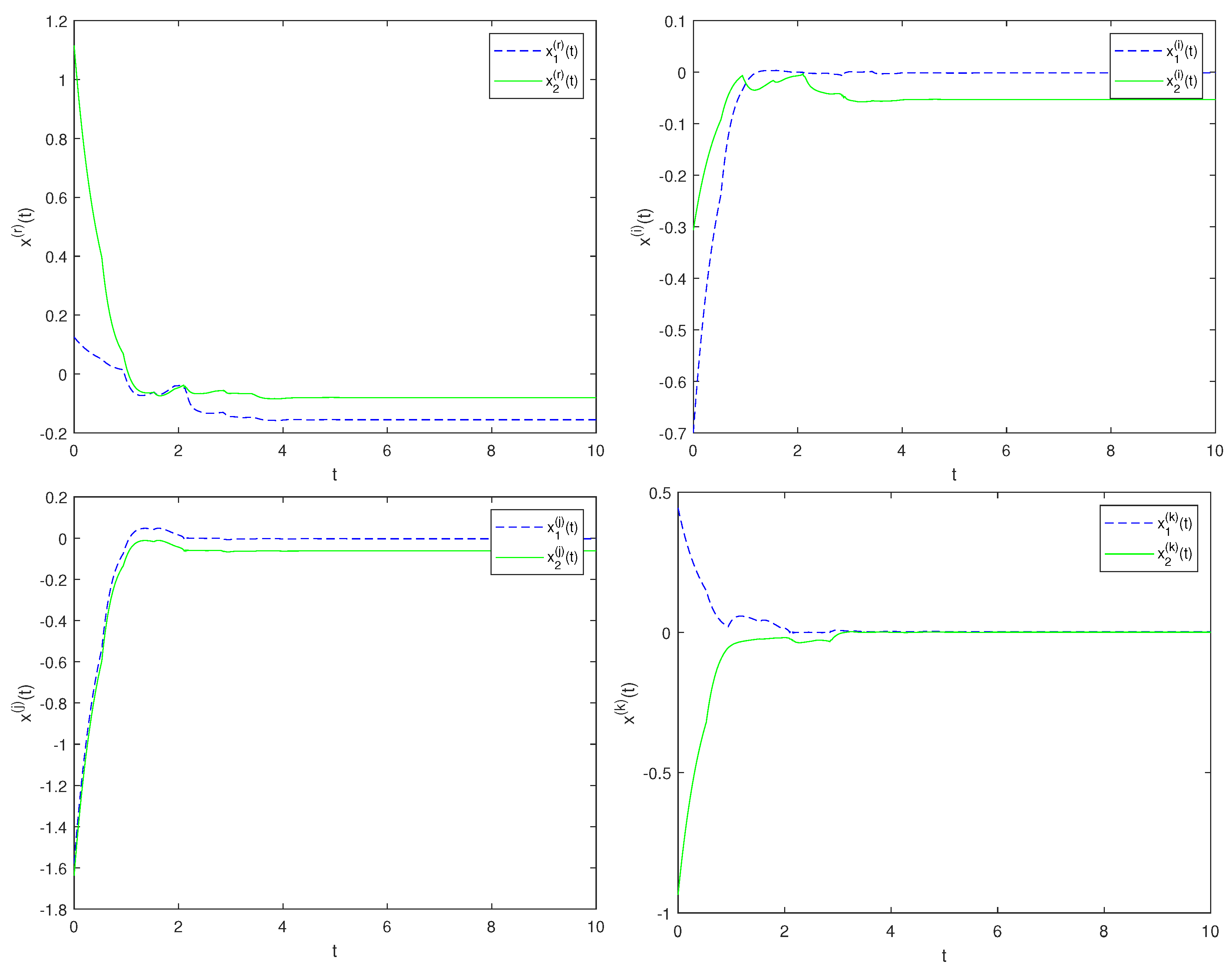
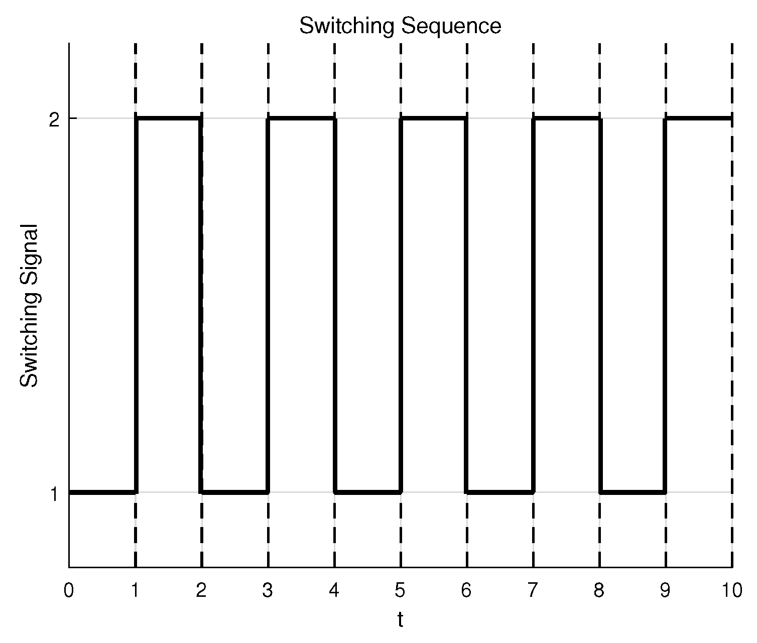
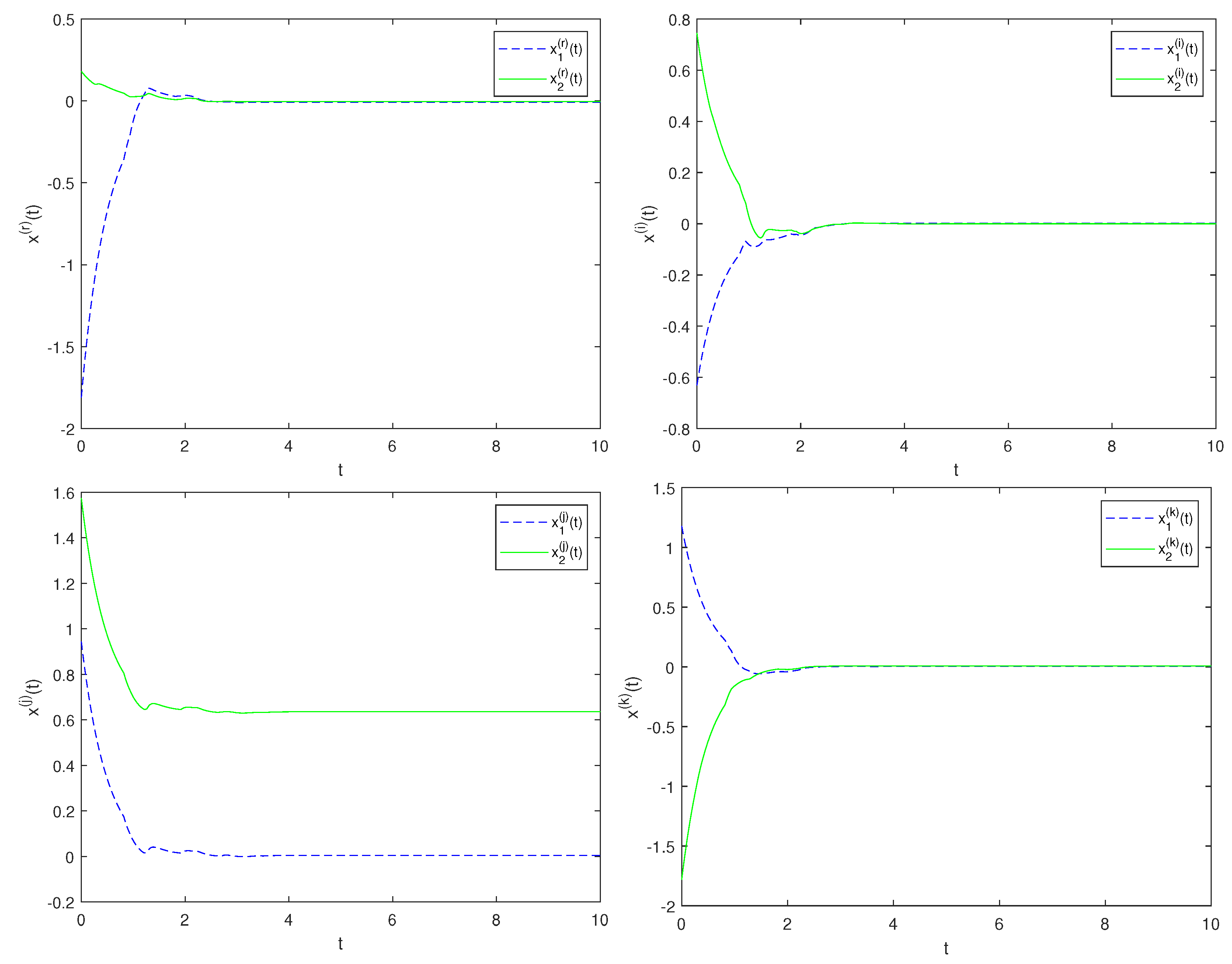
4. Numerical Example

The effective and practical applicability of the proposed method is demonstrated by two comprehensive numerical calculations.

Example 1.

Consider the following GAS of system (3) with two subsystems.

The parameter matrix for subsystem 1 is given below:

$$\begin{array}{cc}\hfill & A_1=\left[\begin{array}{cc}5& 0\\ 0& 5\end{array}\right];\hfill \\ & B_1=\left[\begin{array}{cc}0.3-0.2{\xi }_1-0.2{\xi }_2+0.2{\xi }_3& 0.2+0.2{\xi }_1-0.2{\xi }_2-0.2{\xi }_3\\ 0.2-0.2{\xi }_1+0.2{\xi }_2-0.2{\xi }_3& 0.3+0.2{\xi }_1-0.2{\xi }_2+0.2{\xi }_3\end{array}\right];\hfill \\ & C_1=\left[\begin{array}{cc}0.2-0.3{\xi }_1+0.2{\xi }_{2}j+0.3{\xi }_3& 0.3+0.2{\xi }_1+0.3{\xi }_2-0.1{\xi }_3\\ 0.2+0.4{\xi }_1-0.3{\xi }_2-0.3{\xi }_3& 0.2+0.3{\xi }_1+0.4{\xi }_2+0.3{\xi }_3\end{array}\right];\hfill \\ & D_1=\left[\begin{array}{cc}0.1+0.1{\xi }_1+0.1{\xi }_2-0.1{\xi }_3& 0.1+0.1{\xi }_1-0.1{\xi }_2-0.1{\xi }_3\\ 0.1-0.1{\xi }_1+0.1{\xi }_2-0.1{\xi }_3& 0.1+0.1{\xi }_1-0.1{\xi }_2+0.1{\xi }_3\end{array}\right].\hfill \end{array}$$

The parameter matrix for subsystem 2 is given below:

$$\begin{array}{cc}\hfill & A_2=\left[\begin{array}{cc}4& 0\\ 0& 4\end{array}\right];\hfill \\ & B_2=\left[\begin{array}{cc}0.4-0.3{\xi }_1-0.5{{\rm Y}}_2+0.2{\xi }_3& 0.2+0.4{\xi }_1-0.3{\xi }_2-0.3{\xi }_3\\ 0.4-0.5{\xi }_1+0.2{\xi }_2-0.2{\xi }_3& 0.3+0.2{\xi }_1-0.1{\xi }_2+0.4{\xi }_3\end{array}\right];\hfill \\ & C_2=\left[\begin{array}{cc}0.3-0.2{\xi }_1+0.1{\xi }_2+0.1{\xi }_3& 0.2+0.3{\xi }_1+0.1{\xi }_2-0.2{\xi }_3\\ 0.4+0.2{\xi }_1-0.1{\xi }_2-0.2{\xi }_3& 0.2+0.3{\xi }_1+0.1{\xi }_2+0.3{\xi }_3\end{array}\right];\hfill \\ & D_2=\left[\begin{array}{cc}0.12+0.12{\xi }_1+0.12v_2-0.12{\xi }_3& 0.12+0.12{\xi }_1-0.12{\xi }_2-0.12{\xi }_3\\ 0.12-0.12{\xi }_1+0.12{\xi }_2-0.12{\xi }_3& 0.12+0.12{\xi }_1-0.12{\xi }_2+0.12{\xi }_3\end{array}\right].\hfill \end{array}$$

The remaining parameters of the system are given below:

$$\begin{array}{cc}\hfill & f\left(\mathcal{Ƶ}\left(s\right)\right)=0.18tanh\left(\mathcal{Ƶ}\left(s\right)\right);\delta \left(s\right)=0.45+0.35sin\left(s\right);\varrho \left(s\right)=0.55+0.15sin\left(s\right);\hfill \\ & \delta =0.6;\varrho =0.7;{\delta }_m=0.1;{\delta }_M=0.8;{\varrho }_m=0.4,{\varrho }_M=0.7;{\mathcal{L}}_1=\left[\begin{array}{cc}0.9& 0\\ 0& 0.9\end{array}\right].\hfill \end{array}$$

Applying Theorem 1 and the Matlab toolbox to inequality (4) yields the following feasible solutions.

Feasible solutions for subsystem 1:

$$\begin{array}{cc}\hfill & P_1=\left[\begin{array}{cc}67.6113& 0\\ 0& 67.6113\end{array}\right];Q_{11}=\left[\begin{array}{cc}36.1458& 0\\ 0& 36.1458\end{array}\right];Q_{21}=\left[\begin{array}{cc}70.6581& 0\\ 0& 70.6581\end{array}\right];\hfill \\ & Q_{31}=\left[\begin{array}{cc}9.2745& 0\\ 0& 9.2745\end{array}\right];Q_{41}=\left[\begin{array}{cc}3.9145& 0\\ 0& 3.9145\end{array}\right];R_{11}=\left[\begin{array}{cc}105.1029& 0\\ 0& 105.1029\end{array}\right];\hfill \\ & M_{11}=\left[\begin{array}{cc}-52.2140& 0.1648\\ 0.1648& -52.1176\end{array}\right];M_{21}=\left[\begin{array}{cc}12.5034& 0.2328\\ 0.2328& 12.6901\end{array}\right];M_{31}=\left[\begin{array}{cc}0.1261& 0.3657\\ 0.3657& 0.3097\end{array}\right];\hfill \end{array}$$

Feasible solutions for subsystem 2:

$$\begin{array}{cc}\hfill & P_2=\left[\begin{array}{cc}44.0816& 0\\ 0& 44.0816\end{array}\right];Q_{12}=\left[\begin{array}{cc}22.7387& 0\\ 0& 22.7387\end{array}\right];Q_{22}=\left[\begin{array}{cc}71.0550& 0\\ 0& 71.0550\end{array}\right];\hfill \\ & Q_{32}=\left[\begin{array}{cc}9.0316& 0\\ 0& 9.0316\end{array}\right];Q_{42}=\left[\begin{array}{cc}1.5457& 0\\ 0& 1.5457\end{array}\right];R_{12}=\left[\begin{array}{cc}128.5438& 0\\ 0& 128.5438\end{array}\right];\hfill \\ & M_{12}=\left[\begin{array}{cc}-20.8403& 0.7058\\ 0.7058& -21.9136\end{array}\right];M_{22}=\left[\begin{array}{cc}9.9510& 0.3282\\ 0.3282& 9.5897\end{array}\right];M_{32}=\left[\begin{array}{cc}0.2783& 0.5985\\ 0.5985& 0.6493\end{array}\right];\hfill \end{array}$$

The trend plot of the state variables over time for system (3) with the above parameters is given below:

Remark 5.

In Figure 2, $\mathcal{Ƶ}{\xi }_0\left(s\right),\mathcal{Ƶ}{\xi }_1,\left(s\right),\mathcal{Ƶ}{\xi }_2\left(s\right),\mathcal{Ƶ}{\xi }_3\left(s\right)$ are denoted by $x^{\left(r\right)}\left(t\right),x^{\left(i\right)}\left(t\right),x^{\left(j\right)}\left(t\right),x^{\left(k\right)}\left(t\right)$, respectively. From the above image, it can be seen that the system is divided into four parts, and under any switching law, the trajectories of the state variables gradually converge to a fixed point over time, verifying the effectiveness of the results obtained.

Example 2.

Consider the GES of the following system (3) with two subsystems.

The parameter matrix for subsystem 1 is given below:

$$\begin{array}{cc}\hfill & A_1=\left[\begin{array}{cc}3.5& 0\\ 0& 3.5\end{array}\right];\hfill \\ & B_1=\left[\begin{array}{cc}0.35-0.25{\xi }_1-0.25{\xi }_2+0.25{\xi }_3& 0.25+0.25{\xi }_1-0.25{\xi }_2-0.25{\xi }_3\\ 0.25-0.25{\xi }_1+0.25{\xi }_2-0.25{\xi }_3& 0.35+0.25{\xi }_1-0.25{\xi }_2+0.25{\xi }_3\end{array}\right];\hfill \\ & C_1=\left[\begin{array}{cc}0.25-0.35{\xi }_1+0.25{\xi }_2+0.35{\xi }_3& 0.35+0.25{\xi }_1+0.35{\xi }_2-0.15{\xi }_3\\ 0.25+0.45{\xi }_1-0.35{\xi }_2-0.35{\xi }_3& 0.25+0.35{\xi }_1+0.45{\xi }_2+0.35{\xi }_3\end{array}\right];\hfill \\ & D_1=\left[\begin{array}{cc}0.15+0.15{\xi }_1+0.15{\xi }_2-0.15{\xi }_3& 0.1+0.15{\xi }_1-0.15{\xi }_2-0.15{\xi }_3\\ 0.15-0.15{\xi }_1+0.15{\xi }_2-0.15{\xi }_3& 0.15+0.15{\xi }_1-0.15\xi 2+0.15{\xi }_3\end{array}\right].\hfill \end{array}$$

The parameter matrix for subsystem 2 is given below:

$$\begin{array}{cc}\hfill & A_2=\left[\begin{array}{cc}4.5& 0\\ 0& 4.5\end{array}\right];\hfill \\ & B_2=\left[\begin{array}{cc}0.45-0.35{\xi }_1-0.55{\xi }_2+0.25{\xi }_3& 0.25+0.45{\xi }_1-0.35{\xi }_2-0.35{\xi }_3\\ 0.45-0.55{\xi }_1+0.25{\xi }_2-0.25{\xi }_3& 0.35+0.25{\xi }_1-0.15{\xi }_2+0.45{\xi }_3\end{array}\right];\hfill \\ & C_2=\left[\begin{array}{cc}0.35-0.25{\xi }_1+0.15{\xi }_2+0.15{\xi }_3& 0.25+0.35{\xi }_1+0.15{\xi }_2-0.25{\xi }_3\\ 0.45+0.25{\xi }_1-0.15{\xi }_2-0.25{\xi }_3& 0.25+0.35{\xi }_1+0.15{\xi }_2+0.35{\xi }_3\end{array}\right];\hfill \\ & D_2=\left[\begin{array}{cc}0.1+0.1{\xi }_1+0.1{\xi }_2-0.1{\xi }_3& 0.1+0.1{\xi }_1-0.1{\xi }_2-0.1{\xi }_3\\ 0.1-0.1{\xi }_1+0.1{\xi }_2-0.1{\xi }_3& 0.1+0.1v_1-0.1{\xi }_2+0.1{\xi }_3\end{array}\right].\hfill \end{array}$$

The remaining parameters of the system are given below:

$$\begin{array}{cc}\hfill & f\left(\mathcal{Ƶ}\left(s\right)\right)=0.18tanh\left(\mathcal{Ƶ}\left(s\right)\right);\delta \left(s\right)=1.25+0.75sin\left(s\right);\varrho \left(s\right)=0.75+0.35sin\left(s\right);\hfill \\ & {\mathcal{L}}_2=\left[\begin{array}{cc}0.3& 0\\ 0& 0.3\end{array}\right];{\mathcal{L}}_3=\left[\begin{array}{cc}0.5& 0\\ 0& 0.5\end{array}\right];\hfill \\ & \epsilon =1.1;\rho =0.8;\delta =0.8;\varrho =0.5;{\delta }_M=2;{\delta }_m=0.5;{\varrho }_M=1.1;{\varrho }_m=0.4.\hfill \end{array}$$

Applying Theorem 2 and the Matlab toolbox to inequality (16) yields the following feasible solutions.

Feasible solutions for subsystem 1:

$$\begin{array}{cc}\hfill & P_1=\left[\begin{array}{cc}1.1007& 0\\ 0& 1.1007\end{array}\right];Q_{51}=\left[\begin{array}{cc}1.2674& 0\\ 0& 1.2674\end{array}\right];\hfill \\ & Q_{61}=\left[\begin{array}{cc}2.0343& 0\\ 0& 2.0343\end{array}\right];Q_{71}=\left[\begin{array}{cc}2.9556& 0\\ 0& 2.9556\end{array}\right];\hfill \\ & Q_{81}=\left[\begin{array}{cc}2.2358& 0\\ 0& 2.2358\end{array}\right];R_{21}=\left[\begin{array}{cc}2.9633& 0\\ 0& 2.9633\end{array}\right];\hfill \end{array}$$

$$\begin{array}{cc}\hfill & R_{31}=\left[\begin{array}{cc}8.0982& 0\\ 0& 8.0982\end{array}\right];M_{41}=\left[\begin{array}{cc}1.5591& -1.8255\\ -1.8255& 5.1721\end{array}\right];\hfill \\ & M_{51}=\left[\begin{array}{cc}3.5254& -5.0599\\ -5.0599& 3.2349\end{array}\right];M_{61}=\left[\begin{array}{cc}4.7688& 1.7046\\ 1.7046& 1.8366\end{array}\right];\hfill \end{array}$$

Feasible solutions for subsystem 2:

$$\begin{array}{cc}\hfill & P_2=\left[\begin{array}{cc}5.2007& 0\\ 0& 5.2007\end{array}\right];Q_{52}=\left[\begin{array}{cc}1.0076& 0\\ 0& 1.0076\end{array}\right];\hfill \\ & Q_{62}=\left[\begin{array}{cc}5.4335& 0\\ 0& 5.4335\end{array}\right];Q_{72}=\left[\begin{array}{cc}1.1161& 0\\ 0& 1.1161\end{array}\right];\hfill \\ & Q_{82}=\left[\begin{array}{cc}3.2796& 0\\ 0& 3.2796\end{array}\right];R_{22}=\left[\begin{array}{cc}7.9832& 0\\ 0& 7.9832\end{array}\right];\hfill \\ & R_{32}=\left[\begin{array}{cc}1.2764& 0\\ 0& 1.2764\end{array}\right];M_{42}=\left[\begin{array}{cc}-3.4542& -3.2056\\ -3.2056& -3.5822\end{array}\right];\hfill \\ & M_{52}=\left[\begin{array}{cc}1.1603& -7.1776\\ -7.1776& 1.1593\end{array}\right];M_{62}=\left[\begin{array}{cc}2.1826& 1.5615\\ 1.5615& 1.0790\end{array}\right];\hfill \end{array}$$

By Theorem 2, system (3) with all the above parameters is GES. From switching condition, we know that $S_a>{S_a}^{\divideontimes }={\displaystyle \frac{ln\epsilon }{\rho }}=0.1191$; thus, there is the option of $S_a=0.3>{S_a}^{\divideontimes }$. By means of (31)–(33), one obtains $\mu =0.2809,\beta =1.1007,\alpha =28.4129$, and then, we can obtain the state decay estimate for system (3) with the above parameters as follows:

$$\begin{array}{c}\hfill ∥\mathcal{Ƶ}\left(s\right)∥\le 5.0810e^{-0.2809\left(s-s_0\right)}∥\mathcal{Ƶ}\left(s_0\right)∥.\end{array}$$

The switching sequence diagram is as follows:

In this paper, we consider time-dependent switching. Thus, given a time sequence, switching takes palce at a specified point in time.

A trend plot of the state variables over time for system (3) with the above parameters is given below:

Remark 6.

Figure 4 has the same parameter representation as Figure 2. Combining Figure 3 and Figure 4, it can be seen that even though the switching node is given to allow the system to switch, it does not affect the result that the system eventually stabilizes. It can also be observed from Figure 4 that the system is divided into four parts, all of which eventually converge to stability, verifying the effectiveness of the results obtained.

Remark 7.

Most of the current studies on quaternion-valued neural networks [11,12,13,14] do not consider switching, and studies on switching neural networks [28,30,31,32] do not consider quaternions. Therefore, we try to combine quaternion and switching neural networks by using an undecomposed approach to deal with quaternions while considering both state time-varying time delay and neutral-type time-varying time delay. The activation function we use here is tanh, which is difficult to decompose.

5. Conclusions

This paper investigated the issues of GAS and GES for QVSNNs that simultaneously possess state time-varying delays and neutral-type time-varying delays. An appropriate Lyapunov–Krasovskii functional was proposed, guided by the fundamentals of Lyapunov theorem. The integral quaternion method and the average dwell time method are employed, and by utilizing Wirtinger-based inequality and LMI, combining the theoretical derivation process, it was shown that the considered system is GAS and GES. Additionally, the state decay estimation of the system and a specific case have been provided. Finally, the effective and practical applicability of the proposed method was demonstrated by two comprehensive numerical calculations. Considering that the activation weights of each subsystem vary, the switching probabilities are of paramount importance. Future research efforts will focus on switching probabilities, aiming to overcome this challenging issue.

References

1. Zou, A.M.; Kumar, K.D.; Hou, Z.G. Quaternion-based adaptive output feedback attitude control of spacecraft using Chebyshev neural networks. IEEE Trans. Neural Netw. 2010, 21, 1457–1471. [Google Scholar] [PubMed]
2. Rochefort, D.; De Lafontaine, J.; Brunet, C.A. A new satellite attitude state estimation algorithm using quaternion neural networks. In Proceedings of the AIAA Guidance, Navigation, and Control Conference and Exhibit, San Francisco, CA, USA, 15–18 August 2005; p. 6447. [Google Scholar]
3. Song, Q.; Wu, Q.; Liu, Y. Stabilization of chaotic quaternion-valued neutral-type neural networks via sampled-data control with two-sided looped functional approach. Nonlinear Anal. Model. Control 2024, 29, 1150–1166. [Google Scholar] [CrossRef]
4. Peng, T.; Wu, Y.; Tu, Z.; Alofi, A.; Lu, J. Fixed-time and prescribed-time synchronization of quaternion-valued neural networks: A control strategy involving Lyapunov functions. Neural Netw. 2023, 160, 108–121. [Google Scholar] [CrossRef]
5. Takahashi, K. Remarks on quaternion neural networks with application to trajectory control of a robot manipulator. In Proceedings of the 2019 Australian & New Zealand Control Conference (ANZCC), Auckland, New Zealand, 27–29 November 2019; pp. 116–121. [Google Scholar]
6. Altamirano-Gomez, G.; Gershenson, C. Quaternion Convolutional Neural Networks: Current Advances and Future Directions. Adv. Appl. Clifford Algebr. 2024, 34, 42. [Google Scholar] [CrossRef]
7. Miao, J.; Kou, K.I.; Yang, Y.; Yang, L.; Han, J. Quaternion matrix completion using untrained quaternion convolutional neural network for color image inpainting. Signal Process. 2024, 221, 109504. [Google Scholar] [CrossRef]
8. Zhou, H.; Zhang, X.; Zhang, C.; Ma, Q. Quaternion convolutional neural networks for hyperspectral image classification. Eng. Appl. Artif. Intell. 2023, 123, 106234. [Google Scholar] [CrossRef]
9. Kumar, S.; Rastogi, U. A comprehensive review on the advancement of high-dimensional neural networks in quaternionic domain with relevant applications. Arch. Comput. Methods Eng. 2023, 30, 3941–3968. [Google Scholar] [CrossRef]
10. Hirose, A.; Shang, F.; Otsuka, Y.; Natsuaki, R.; Matsumoto, Y.; Usami, N.; Song, Y.; Chen, H. Quaternion Neural Networks: A physics-incorporated intelligence framework [Hypercomplex Signal and Image Processing]. IEEE Signal Process. Mag. 2024, 41, 88–100. [Google Scholar] [CrossRef]
11. Wang, H.; Tan, J.; Wen, S. Exponential stability analysis of mixed delayed quaternion-valued neural networks via decomposed approach. IEEE Access 2020, 8, 91501–91509. [Google Scholar] [CrossRef]
12. Humphries, U.; Rajchakit, G.; Kaewmesri, P.; Chanthorn, P.; Sriraman, R.; Samidurai, R.; Lim, C.P. Stochastic memristive quaternion-valued neural networks with time delays: An analysis on mean square exponential input-to-state stability. Mathematics 2020, 8, 815. [Google Scholar] [CrossRef]
13. Yang, X.; Li, C.; Song, Q.; Li, H.; Huang, J. Effects of state-dependent impulses on robust exponential stability of quaternion-valued neural networks under parametric uncertainty. IEEE Trans. Neural Netw. Learn. Syst. 2018, 30, 2197–2211. [Google Scholar] [CrossRef] [PubMed]
14. Shu, J.; Wu, B.; Xiong, L. Stochastic stability criteria and event-triggered control of delayed Markovian jump quaternion-valued neural networks. Appl. Math. Comput. 2022, 420, 126904. [Google Scholar] [CrossRef]
15. Chen, X.; Li, Z.; Song, Q.; Hu, J.; Tan, Y. Robust stability analysis of quaternion-valued neural networks with time delays and parameter uncertainties. Neural Netw. 2017, 91, 55–65. [Google Scholar] [CrossRef]
16. Song, Q.; Chen, Y.; Zhao, Z.; Liu, Y.; Alsaadi, F.E. Robust stability of fractional-order quaternion-valued neural networks with neutral delays and parameter uncertainties. Neurocomputing 2021, 420, 70–81. [Google Scholar] [CrossRef]
17. You, X.; Song, Q.; Liang, J.; Liu, Y.; Alsaadi, F.E. Global μ-stability of quaternion-valued neural networks with mixed time-varying delays. Neurocomputing 2018, 290, 12–25. [Google Scholar] [CrossRef]
18. Wu, L.; Feng, Z.; Lam, J. Stability and synchronization of discrete-time neural networks with switching parameters and time-varying delays. IEEE Trans. Neural Netw. Learn. Syst. 2013, 24, 1957–1972. [Google Scholar] [CrossRef]
19. Shen, W.; Zeng, Z.; Wang, L. Stability analysis for uncertain switched neural networks with time-varying delay. Neural Netw. 2016, 83, 32–41. [Google Scholar] [CrossRef]
20. Liu, C.; Yang, Z.; Sun, D.; Liu, X.; Liu, W. Stability of switched neural networks with time-varying delays. Neural Comput. Appl. 2018, 30, 2229–2244. [Google Scholar] [CrossRef]
21. Tu, Z.; Zhao, Y.; Ding, N.; Feng, Y.; Zhang, W. Stability analysis of quaternion-valued neural networks with both discrete and distributed delays. Appl. Math. Comput. 2019, 343, 342–353. [Google Scholar] [CrossRef]
22. Wang, Y.; Niu, B.; Wang, H.; Alotaibi, N.; Abozinadah, E. Neural network-based adaptive tracking control for switched nonlinear systems with prescribed performance: An average dwell time switching approach. Neurocomputing 2021, 435, 295–306. [Google Scholar] [CrossRef]
23. Yang, X.; Liu, Y.; Cao, J.; Rutkowski, L. Synchronization of coupled time-delay neural networks with mode-dependent average dwell time switching. IEEE Trans. Neural Netw. Learn. Syst. 2020, 31, 5483–5496. [Google Scholar] [CrossRef] [PubMed]
24. Sun, J.; Han, J.; Liu, P.; Wang, Y. Memristor-based neural network circuit of pavlov associative memory with dual mode switching. AEU-Int. J. Electron. Commun. 2021, 129, 153552. [Google Scholar] [CrossRef]
25. Chen, Z.; Niu, B.; Zhang, L.; Zhao, J.; Ahmad, A.M.; Alassafi, M.O. Command filtering-based adaptive neural network control for uncertain switched nonlinear systems using event-triggered communication. Int. J. Robust Nonlinear Control 2022, 32, 6507–6522. [Google Scholar] [CrossRef]
26. Dong, Z.; Wang, X.; Zhang, X.; Hu, M.; Dinh, T.N. Global exponential synchronization of discrete-time high-order switched neural networks and its application to multi-channel audio encryption. Nonlinear Anal. Hybrid Syst. 2023, 47, 101291. [Google Scholar] [CrossRef]
27. Wang, H.; Yang, X.; Xiang, Z.; Tang, R.; Ning, Q. Synchronization of switched neural networks via attacked mode-dependent event-triggered control and its application in image encryption. IEEE Trans. Cybern. 2022, 53, 5994–6003. [Google Scholar] [CrossRef]
28. Bao, Y.; Zhang, Y.; Zhang, B. Resilient fixed-time stabilization of switched neural networks subjected to impulsive deception attacks. Neural Netw. 2023, 163, 312–326. [Google Scholar] [CrossRef] [PubMed]
29. Guo, Z.; Liu, L.; Wang, J. Multistability of switched neural networks with piecewise linear activation functions under state-dependent switching. IEEE Trans. Neural Netw. Learn. Syst. 2018, 30, 2052–2066. [Google Scholar] [CrossRef]
30. Jiao, T.; Park, J.H.; Zong, G.; Zhao, Y.; Du, Q. On stability analysis of random impulsive and switching neural networks. Neurocomputing 2019, 350, 146–154. [Google Scholar] [CrossRef]
31. Yang, D.; Li, X. Robust stability analysis of stochastic switched neural networks with parameter uncertainties via state-dependent switching law. Neurocomputing 2021, 452, 813–819. [Google Scholar] [CrossRef]
32. Wu, L.; Feng, Z.; Zheng, W.X. Exponential stability analysis for delayed neural networks with switching parameters: Average dwell time approach. IEEE Trans. Neural Netw. 2010, 21, 1396–1407. [Google Scholar]
33. Tu, Z.; Yang, X.; Wang, L.; Ding, N. Stability and stabilization of quaternion-valued neural networks with uncertain time-delayed impulses: Direct quaternion method. Phys. A Stat. Mech. Its Appl. 2019, 535, 122358. [Google Scholar] [CrossRef]
34. Zeng, H.B.; He, Y.; Wu, M.; Xiao, S.P. Stability analysis of generalized neural networks with time-varying delays via a new integral inequality. Neurocomputing 2015, 161, 148–154. [Google Scholar] [CrossRef]
35. Chen, Z.W.; Yang, J.; Zhong, S.M. Delay-partitioning approach to stability analysis of generalized neural networks with time-varying delay via new integral inequality. Neurocomputing 2016, 191, 380–387. [Google Scholar] [CrossRef]
36. Peng, T.; Qiu, J.; Lu, J.; Tu, Z.; Cao, J. Finite-time and fixed-time synchronization of quaternion-valued neural networks with/without mixed delays: An improved one-norm method. IEEE Trans. Neural Netw. Learn. Syst. 2021, 33, 7475–7487. [Google Scholar] [CrossRef]
37. Syed Ali, M.; Hymavathi, M.; Saroha, S.; Krishna Moorthy, R. Global asymptotic stability of neutral type fractional-order memristor-based neural networks with leakage term, discrete and distributed delays. Math. Methods Appl. Sci. 2021, 44, 5953–5973. [Google Scholar] [CrossRef]
38. Subramanian, K.; Muthukumar, P. Global asymptotic stability of complex-valued neural networks with additive time-varying delays. Cogn. Neurodynamics 2017, 11, 293–306. [Google Scholar] [CrossRef]
39. Liu, Y.; Zhang, D.; Lu, J. Global exponential stability for quaternion-valued recurrent neural networks with time-varying delays. Nonlinear Dyn. 2017, 87, 553–565. [Google Scholar] [CrossRef]
40. Xia, Y.; Chen, X.; Lin, D.; Li, B.; Yang, X. Global exponential stability analysis of commutative quaternion-valued neural networks with time delays on time scales. Neural Process. Lett. 2023, 55, 6339–6360. [Google Scholar] [CrossRef]
41. Li, X.; Pal, N.R.; Li, H.; Huang, T. Intermittent event-triggered exponential stabilization for state-dependent switched fuzzy neural networks with mixed delays. IEEE Trans. Fuzzy Syst. 2021, 30, 3312–3321. [Google Scholar] [CrossRef]
42. Zhan, T.; Ma, S.; Li, W.; Pedrycz, W. Exponential stability of fractional-order switched systems with mode-dependent impulses and its application. IEEE Trans. Cybern. 2021, 52, 11516–11525. [Google Scholar] [CrossRef]
43. Xiao, H.; Zhu, Q.; Karimi, H.R. Stability of stochastic delay switched neural networks with all unstable subsystems: A multiple discretized Lyapunov-Krasovskii functionals method. Inf. Sci. 2022, 582, 302–315. [Google Scholar] [CrossRef]
Figure 1. Diagram of model (3).
Symmetry 17 00979 g001
Figure 2. Response curves over time for x r t , x i t , x j t , and x k t of system (3).
Symmetry 17 00979 g002
Figure 3. Switching sequence diagrams.
Symmetry 17 00979 g003
Figure 4. Response curves over time for x r t , x i t , x j t , and x k t of system (3).
Symmetry 17 00979 g004
Disclaimer/Publisher’s Note: The statements, opinions and data contained in all publications are solely those of the individual author(s) and contributor(s) and not of MDPI and/or the editor(s). MDPI and/or the editor(s) disclaim responsibility for any injury to people or property resulting from any ideas, methods, instructions or products referred to in the content.