Matching Concepts of m-Polar Fuzzy Incidence Graphs

Abstract

The m-Polar Fuzzy Incidence Graph (m-PFIG) is an extension of the m-Polar Fuzzy Graph (m-PFG), which provides information on how vertices affect edges. This study explores the concept of matching within both bipartite and general m-polar fuzzy incidence graphs (m-PFIGs). It extends various results and theorems from fuzzy graph theory to the framework of m-PFIGs. This research investigates various operations within m-PFIGs, including augmenting paths, matching principal numbers, and the relationships among them. It focuses on identifying the most suitable employees for specific roles and achieving optimal outcomes, particularly in situations involving internal conflicts within an organization. To address fuzzy maximization problems involving vertex–incidence pairs, this study outlines key properties of maximum matching principal numbers in m-PFIGs. Ultimately, the matching concept is applied to attain these maximum principal values, demonstrating its effectiveness, particularly in bipartite m-PFIG scenarios.

1. Introduction

1.1. Context and Prior Research

Fuzzy Graph (FG) theory has become a vital tool in the advancement of modern technologies. It is widely utilized in the creation of expert systems, especially those based on rule-driven methodologies within engineering domains. More broadly, graph theory proves to be highly valuable across numerous fields, including mathematics, geometry, topology, computer science, numerical methods, optimization, and operations research, where it is particularly useful for analyzing and representing connectivity.

The idea of incorporating fuzziness to represent uncertainty in real-world scenarios was first introduced by Zadeh in 1965 through fuzzy set theory, which significantly influenced developments in science and technology [1]. Building on this, Zhang [2] expanded the concept by proposing bipolar fuzzy sets (BFS) and exploring their applications in environmental studies [3]. The foundational work on fuzzy graphs began with Kaufman [4], and Rosenfeld [5] further developed the theory by defining fundamental elements such as paths, cycles, and connectedness within fuzzy graphs. Numerous contributions have been made to this area over time [6], particularly through the introduction of new definitions and practical applications [7]. Further advances came from Mordeson and Mathew [8], who played a vital role in generalizing fuzzy graph theory, while Cheng and Nair [9] introduced the idea of fuzzy cliques. Mathew et al. [10] were the first to discuss the notion of saturation in fuzzy graphs. The concept of m-polar fuzzy graphs (m-PFGs) was initially presented by Chen et al. [11], and later, Ghorai and Pal [12] enhanced this area by exploring properties such as density and fuzzy planarity [13]. They also investigated structural aspects such as faces and duality in m-PFGs [14]. Akram et al. [15,16] investigated the edge characteristics of m-polar fuzzy graphs (m-PFGs). A generalized model of m-polar fuzzy graphs (Gm-PFGs), developed to overcome the limitations of the minimum-only relationship framework and to enable the incorporation of maximum, average, and other relationships, has been proposed in [17]. It explores the properties of Gm-PFGs, including their planarity and duality, and presents an application in social network analysis. In [18], the concepts of $\alpha$-saturation and $\beta$-saturation in m-polar fuzzy graphs (m-PFGs), along with their properties, bounds, and structural implications, are discussed. A real-world allocation problem is also modeled using saturated m-PFGs to demonstrate their practical applicability. Isometry in m-polar fuzzy graphs (m-PFGs), including antipodal m-PFGs and the analysis of their metric properties, edge regularity, and structural behavior, is discussed in [19]. A real-life application in road network systems using the $\mu$-distance concept is also demonstrated. The work in [20] defines the interval-valued m-polar fuzzy competition graph (IVm-PFCG) and its variants, explores their structural properties based on interval-valued membership, presents neighborhood-based generalizations, and applies the model to a real-world competitive sector. Moreover, Subrahmanyam [21] proposed various product operations on m-PFGs.

In both fuzzy graph (FG) theory and conventional graph theory, matching is essential. Shen and Tsai [22] were the first to suggest the use of optimal graph matching to solve task assignment problems. The idea of matching within fuzzy graphs was further advanced by Ramakrishnan and Vaidyanathan [23]. Mohan and Gupta then developed a graph matching method specifically for assigning tasks [24]. Khalili et al. [25] contributed to the theoretical foundations by investigating the matching numbers in fuzzy graphs. The concept of bipolar fuzzy incidence graphs (BFIGs) expands upon traditional bipolar fuzzy graphs by integrating vertex–edge relationships. In this context, matching concepts applicable to both bipartite and general BFIGs are introduced, along with extensions of classical fuzzy graph theorems, as discussed in [26]. Key operations, including augmenting paths and matching principal numbers, are examined to support optimal selection scenarios, such as candidate–job pairing and enhancing organizational efficiency. Furthermore, the study illustrates the practical application of maximum matching in addressing fuzzy maximization problems that involve vertex–incidence pairs. The concept of antipodal bipolar fuzzy graphs and their characterizations in the context of complete and strong bipolar fuzzy graphs have been discussed in [27]. The study also examines isomorphic properties and introduces the notion of self-median bipolar fuzzy graphs.

Inspired by [26], we developed our current study. The main objective of this research is to identify the maximum matching principal numbers in mPFIGs. Additionally, we analyze various properties and bounds related to matching in mPFIGs. This work presents a thorough exploration of matchings in mPFIGs, supported by relevant examples.

1.2. Symbols and Notations

Within this section, we introduce and define key notations essential for the development of the theories presented throughout the paper. Table 1 outlines these notations and their respective meanings for clarity and reference.

Table 1. Certain terms are abbreviated in the form of acronyms.

Full Name	Aberration Form
Fuzzy graph	FG
Incidence strength	IS
Incidence strength of connectedness	ISC
Underlying crisp graph	UCG
Membership value	MV
m-Polar fuzzy	m-PF
m-polar fuzzy incidence	m-PFI
m-polar fuzzy set	m-PFS
m-polar fuzzy graph	m-PFG
m-polar fuzzy incidence graph	m-PFIG
m-polar fuzzy incidence subgraph	m-PFIS
Matching principal number	MPN
Matching m-polar fuzzy incidence principal numbers	MmPFIPNs
Maximum matching principal number	MMPN
Neighborly total irregular FG	NTIFG
Highly irregular FG	HIFG
m-polar fuzzy incidence number	mPFIN
Maximum matching m-polar fuzzy incidence number	MMm-PFIN
Maximum matching edge m-polar fuzzy incidence number	MMEm-PFIN
Maximum matching vertex m-polar fuzzy incidence number	MMVm-PFIN
Maximum matching crisp number	MMCN
Bipartite m-polar fuzzy incidence graph	BmPFIG
Augmenting track	AT
Symmetric difference	SD
Neighborhood degree	ND

Section 2 introduces essential preliminary definitions that serve as a foundation for the subsequent sections. Section 3 presents several definitions, examples, results, and theorems related to m-PFIGs. Section 4 continues this exploration with additional relevant definitions, illustrative examples, and theoretical results concerning the matching concept in m-PFIGs. In Section 5, mathematical models are developed to determine MMVm-PFIN in m-PFIGs. Section 6 summarizes the conclusions and outlines potential directions for future research.

2. Preliminaries

This section includes foundational definitions. In this paper, the set ${[0,1]}^m$ represents a partially ordered set (poset) under the pointwise order relation ≤, where m is a natural number. Specifically, for any $a,b\in {[0,1]}^m$, the relation $a\le b$ holds if and only if $p_i\left(a\right)\le p_i\left(b\right)\mathrm{for}\mathrm{all}i=1,2,\dots ,m,$ where $p_i:{[0,1]}^m\to [0,1]$ denotes the i-th projection mapping.

Definition 1 

([5]). An FG $G=(W,\tau ,\nu )$ of the UCG $G^{\ast }=(W,F)$ is defined by $\tau :W\to [0,1]$ and $\nu :W\times W\to [0,1]\mathit{such}\mathit{that}\forall a,b\in W,\nu \left(ab\right)\le \tau \left(a\right)\wedge \tau \left(b\right)$, where $\tau \left(a\right)$ and $\nu (a,b)$ represent the membership values of the vertex a and the edge $(a,b)$ in G, respectively, and ′∧′ denotes the minimum value.

Definition 2 

([12]). An m-polar fuzzy set (or a ${[0,1]}^m$-set) on a set W is a mapping $\tau :W\to {[0,1]}^m$. The collection of all m-polar fuzzy sets on W is denoted by $\mathfrak{m}\left(W\right)$. An m-polar fuzzy relation on τ is an m-polar fuzzy set ν on $W\times W$ such that $\nu (a,b)\le min\left\{\tau \right(a),\tau (b\left)\right\}\mathit{for}\mathit{all}a,b\in W;$ that is, for each $i=1,2,\dots ,m$ and for all $a,b\in W$, $p_i\circ \nu (a,b)\le min\{p_i\circ \tau \left(a\right),p_i\circ \tau \left(b\right)\},$ where $p_i:{[0,1]}^m\to [0,1]$ denotes the i-th projection mapping.

Definition 3 

([20]). An m-polar fuzzy graph (m-PFG) of a graph $G^{\ast }=(W,F)$ is a triplet $G=(W,\tau ,\nu )$, where $\tau :W\to {[0,1]}^m$ is an m-polar fuzzy set on W and $\nu :W\times W\to {[0,1]}^m$ is an m-polar fuzzy set on $W\times W$ such that $\nu (a,b)\le \tau \left(a\right)\wedge \tau \left(b\right)\mathit{for}\mathit{all}a,b\in W, \mathit{and}\nu (a,b)=0$$\mathit{for}\mathit{all}(a,b)\in (W\times W)\setminus F.$

Definition 4 

([12]). The structure $H=(W,\tau ,\nu )$ is defined as a complete m-dimensional PFG if, for all $x_1,w_1\in W$ and for each $i=1,2,\dots ,m$, the following condition holds:

$$p_i\circ \nu (x_1,w_1)=p_i\circ \tau \left(x_1\right)\wedge p_i\circ \tau \left(w_1\right).$$

Definition 5 

([12]). The m-PF strong graph $H=(W,\tau ,\nu )$ is identified when $p_i\circ \nu (x_1,w_1)=p_i\circ \tau \left(x_1\right)\wedge p_i\circ \tau \left(w_1\right)$ holds for each $(x_1,w_1)\in F_1$ and $i=1,2,\dots ,m$.

Definition 6 

([12]). Let $G_1=(W_1^{\prime },{\tau }_1,{\nu }_1)$ and $G_2=(W_2^{\prime },{\tau }_2,{\nu }_2)$ represent two m-dimensional PFGs (Polar Fuzzy Graphs) corresponding to the UCGs $G_1^{\ast }=(W_1,F_1)$ and $G_2^{\ast }=(W_2,F_2)$, respectively. A homomorphism from $G_1$ to $G_2$ is defined as a mapping $\varphi :W_1\to W_2$ that satisfies the following conditions for all $a_1\in W_1$, $(a_1,b_1)\in F_1$, and $i=1,2,\dots ,m$: $p_i\circ {\tau }_1\left(a_1\right)\le p_i\circ {\tau }_2\left(\varphi \left(a_1\right)\right)$ and $p_i\circ {\nu }_1(a_1,b_1)\le p_i\circ {\nu }_2(\varphi \left(a_1\right),\varphi \left(b_1\right)).$ This definition ensures that the structural and functional properties of $G_1$ are maintained through the mapping ϕ.

Definition 7 

([14]). Let $G_1=(W_1,{\tau }_1,{\nu }_1)$ and $G_2=(W_2,{\tau }_2,{\nu }_2)$ be two m-polar fuzzy graphs (mPFGs). A homomorphism between $G_1$ and $G_2$ is a mapping $\varphi :W_1\to W_2$ satisfying the following conditions for each $i=1,2,\dots ,m:p_i\circ {\tau }_1\left(a_1\right)\le p_i\circ {\tau }_2\left(\varphi \left(a_1\right)\right)$ $\mathit{for}\mathit{all}{a}_1\in W_1,\mathit{and}$ $p_i\circ {\nu }_1\left(a_1{b}_1\right)\le p_i\circ {\nu }_2\left(\varphi \left(a_1\right)\varphi \left(b_1\right)\right)\mathit{for}\mathit{all}{a}_1,b_1\in W_1.$

Definition 8 

([13]). For two m-dimensional PFGs $G_1$ and $G_2$, a bijective homomorphism is defined as a mapping $g:W_1\to W_2$ that satisfies the condition $p_i\circ {\nu }_1(x_1,y_1)=p_i\circ {\nu }_2(g\left(x_1\right),g\left(y_1\right)),$ for all $(x_1,y_1)\in F_1$ and $i=1,2,\dots ,m$. This mapping is referred to as a coweak isomorphism or a (weak) line isomorphism. A mapping f is called an isomorphism between $G_1$ and $G_2$ if it serves as both a (weak) line-isomorphism and a (weak) vertex-isomorphism between them.

Definition 9 

([14]). For an m-PFG, if an edge $(u,v)$, where $u,v\in W$ is said to be independently strong if it satisfies the condition $p_i\circ \nu (u,v)\ge {\displaystyle \frac{1}{2}}\left\{p_i\circ \tau \left(u\right)\wedge p_i\circ \tau \left(v\right)\right\},i=1,2,\dots ,m$, holds for $G=(W,\tau ,\nu )$; otherwise, it is called an independently weak edge.

Definition 10 

([14]). The strength of the edge $(u,v)$ can be expressed as

$p_i\circ J(u,v)={\displaystyle \frac{p_i\circ \nu (u,v)}{p_i\circ \tau \left(u\right)\wedge p_i\circ \tau \left(v\right)}},$ for $i=1,2,\dots ,m$.

Definition 11 

([15]). Let $G=(W,\tau ,\nu )$ be an m-PFG with UCG $G^{\ast }=(W,F)$. Consider a subgraph $Q=(W_1,{\tau }_1,{\nu }_1)$ of G with UCG $Q^{\ast }=(W_1,F_1)$ that is a subgraph of G. If the pair $(supp\left(W_1\right),supp\left(F_1\right))$ forms a cycle, and there is no uniquely existing edge $(u,v)\in F_1$ such that $p_i\circ \nu (u,w)=inf\{p_i\circ \nu (b,d):(b,d)\in F_1\},$ for $i=1,2,\dots ,m$, then Q is called an m-PFG cycle.

Definition 12 

([20]). Let $H=(W,\tau ,\nu )$ be an m-PFG, and let $P:d_1,d_2,\dots ,d_k$ be a path in H. The strength of path P, denoted by $S\left(P\right)$, can be determined as follows:

$$S\left(P\right)=\left(\underset{1\le i<j\le k}{min}{p}_1\circ \nu (d_i,d_j),\underset{1\le i<j\le k}{min}{p}_2\circ \nu (d_i,d_j),\dots ,\underset{1\le i<j\le k}{min}{p}_m\circ \nu (d_i,d_j)\right),$$

which is also written as $S\left(P\right)=({\nu }_1^n(d_i,d_j),{\nu }_2^n(d_i,d_j),\dots ,{\nu }_m^n(d_i,d_j)).$ The strength connection (SC) between $d_1$ and $d_k$ is given by

$$CON{N}_G(d_1,d_k)=\left(p_1\circ \nu {(d_i,d_j)}^{\infty },p_2\circ \nu {(d_i,d_j)}^{\infty },\dots ,p_m\circ \nu {(d_i,d_j)}^{\infty }\right),$$

where $(p_s\circ \nu {(a,d)}^{\infty })={max}_{n\in \mathbb{N}}\left({\nu }_i^n(a,d)\right)$.

Definition 13 

([6]). If there is a spanning m-PF subgraph $H=(V,{\tau }^{\prime },{\nu }^{\prime })$ that is also an m-PF tree, and for each $s=1$ to m, then a graph $G=(V,\tau ,\nu )$ is called an m-PF tree. $p_s\circ {\nu }^{\prime }(a,d)=0$ implies that $p_s\circ {\nu }^{\prime }(a,d)>p_s\circ CON{N}_H(a,d)$.

Definition 14 

([6]). Let $H=(W,\tau ,\nu )$ be an n-PFG. An edge $(x,y)$ is referred to as an n-PF bridge if its removal results in an increase in the shortest communication path between some other pair of vertices in H.

Definition 15 

([15]). Let $G=(W,\tau ,\nu )$ be an n-dimensional PFG. The n-dimensional open neighborhood of a vertex y, denoted $\mathcal{N}\left(y\right)$, is given by $\mathcal{N}\left(y\right)=\{w\in W:(y,w)\in F\}.$ The closed neighborhood of a vertex y, represented as $\mathcal{N}\left[y\right]$, is defined as $\mathcal{N}\left[y\right]=\mathcal{N}\left(y\right)\cup \left\{y\right\}.$

3. $\mathbf{m}$-Polar Fuzzy Incidence Graph

In this part, we will present m-PFIG and explore its characteristics. Additionally, we will outline the resources of m-PFIS, supported by illustration.

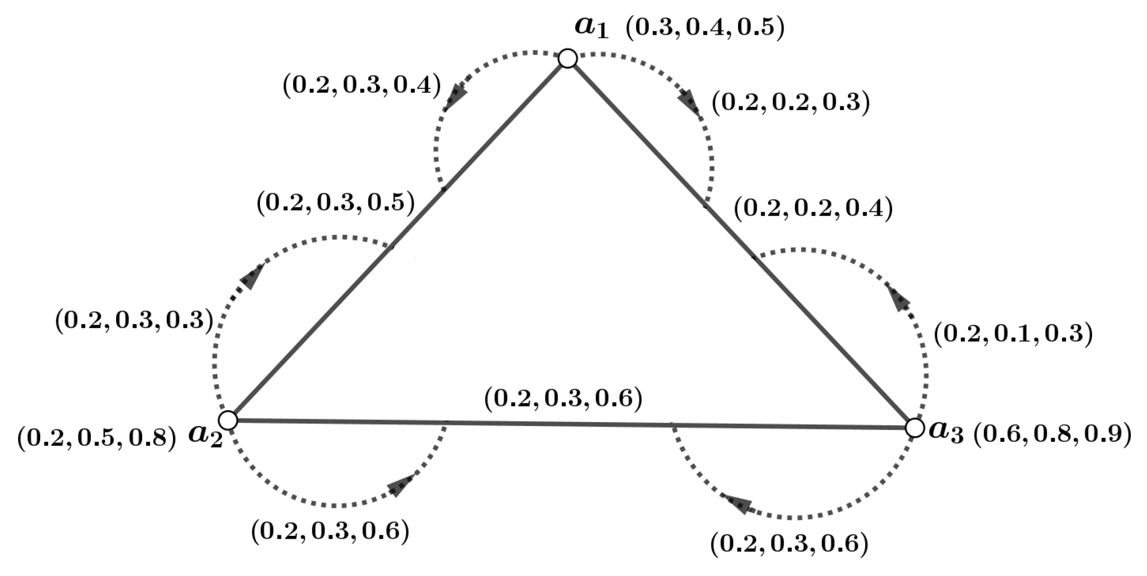
Definition 16. 

Let $G=(W,\tau ,\nu )$ be an m-dimensional PFG, where its associated crisp graph is denoted as $G^{\ast }=(W,F)$. Here, $\tau :W\to {[0,1]}^m$ represents an m-PFS on W, and $\nu :W\times W\to {[0,1]}^m$ defines an m-PFS on $W\times W$. A mapping $\psi :W\times F\to {[0,1]}^m$ is then defined as follows:

$$p_i\circ \psi (y,(y,z))\le min\{p_i\circ \tau \left(y\right),p_i\circ \nu (y,z)\}$$

for $i=1,2,\dots ,m$, $y\in W$, and $(y,z)\in F$. The terms $p_i\circ \tau \left(y\right)$ and $p_i\circ \nu (y,z)$ represent the $i\mathbf{th}$ membership degree for the vertex y and the edge $(y,z)$, respectively, in the m-PFG. The mapping ψ is referred to as the m-PFI of $\tilde{G}$, while the structure $\tilde{G}=(W,\tau ,\nu ,\psi )$ is recognized as the m-PFIG. Figure 1 shows an example.

Figure 1. An illustration of an m-Polar Fuzzy Incidence Graph (m-PFIG).

Definition 17. 

An m-dimensional PFIG $\tilde{H}=(W_1,{\tau }_1,{\nu }_1,{\psi }_1)$ is defined as a partial subgraph of another m-dimensional PFIG $\tilde{G}=(W,\tau ,\nu ,\psi )$ if the following conditions hold for every $y\in W$, $(y,z)\in F$, and $i=1,2,\dots ,m$: $p_i\circ {\tau }_1\left(y\right)\le p_i\circ \tau \left(y\right),p_i\circ {\nu }_1(y,z)\le p_i\circ \nu (y,z),\mathit{and}{p}_i\circ {\psi }_1(y,(y,z))\le p_i\circ \psi (y,(y,z)).$ Furthermore, $\tilde{H}$ is considered a subgraph of $\tilde{G}$ and is denoted as an m-PFIS if $W_1\subseteq W$, $F_1\subseteq F$, ${\psi }_1\subseteq \psi$, and for all $y\in W$ and $(y,z)\in F$, the equalities $p_i\circ {\tau }_1\left(y\right)=p_i\circ \tau \left(y\right),p_i\circ {\nu }_1(y,z)=p_i\circ \nu (y,z),\mathit{and}{p}_i\circ {\psi }_1(y,(y,z))=p_i\circ \psi (y,(y,z))$ are satisfied.

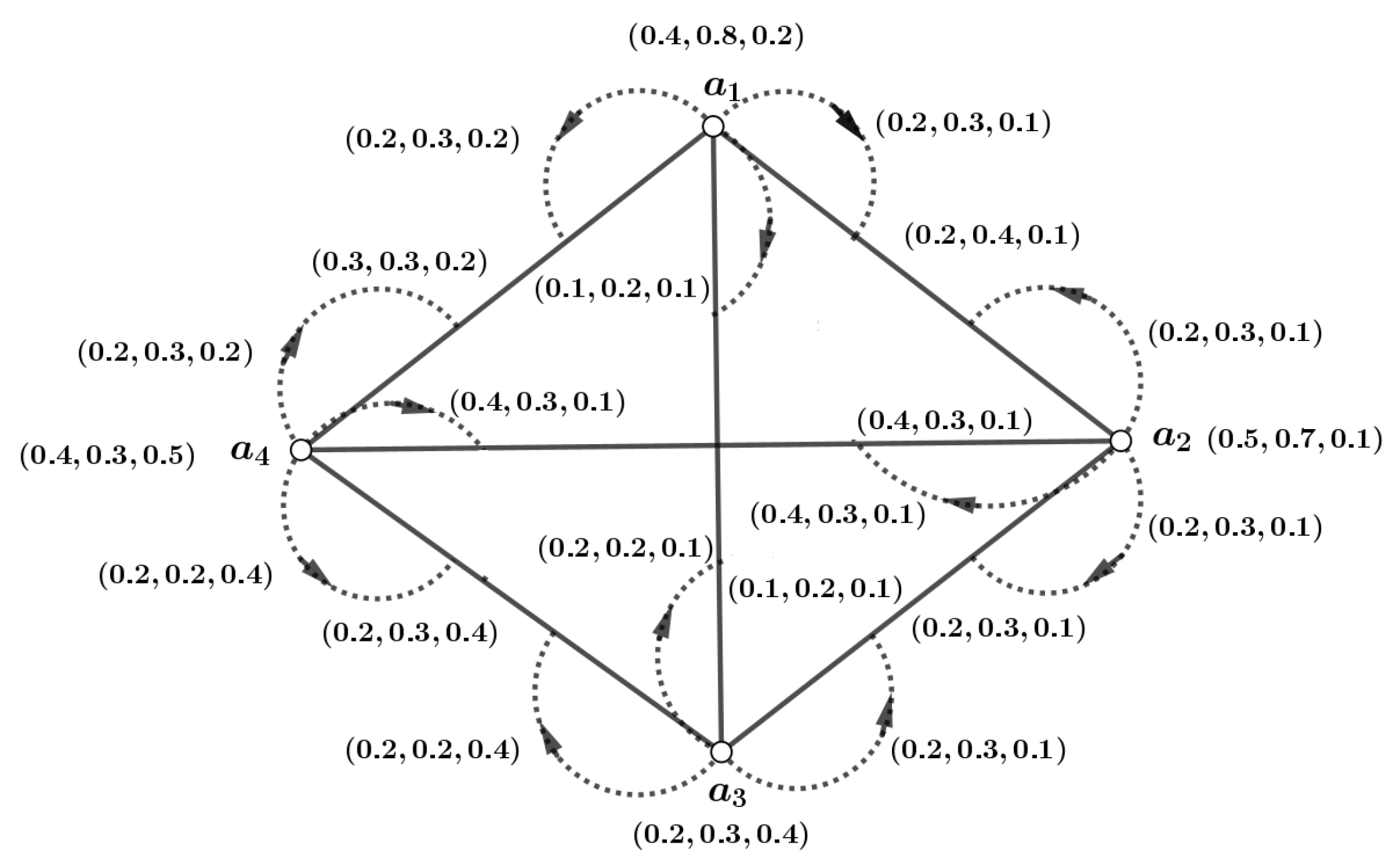
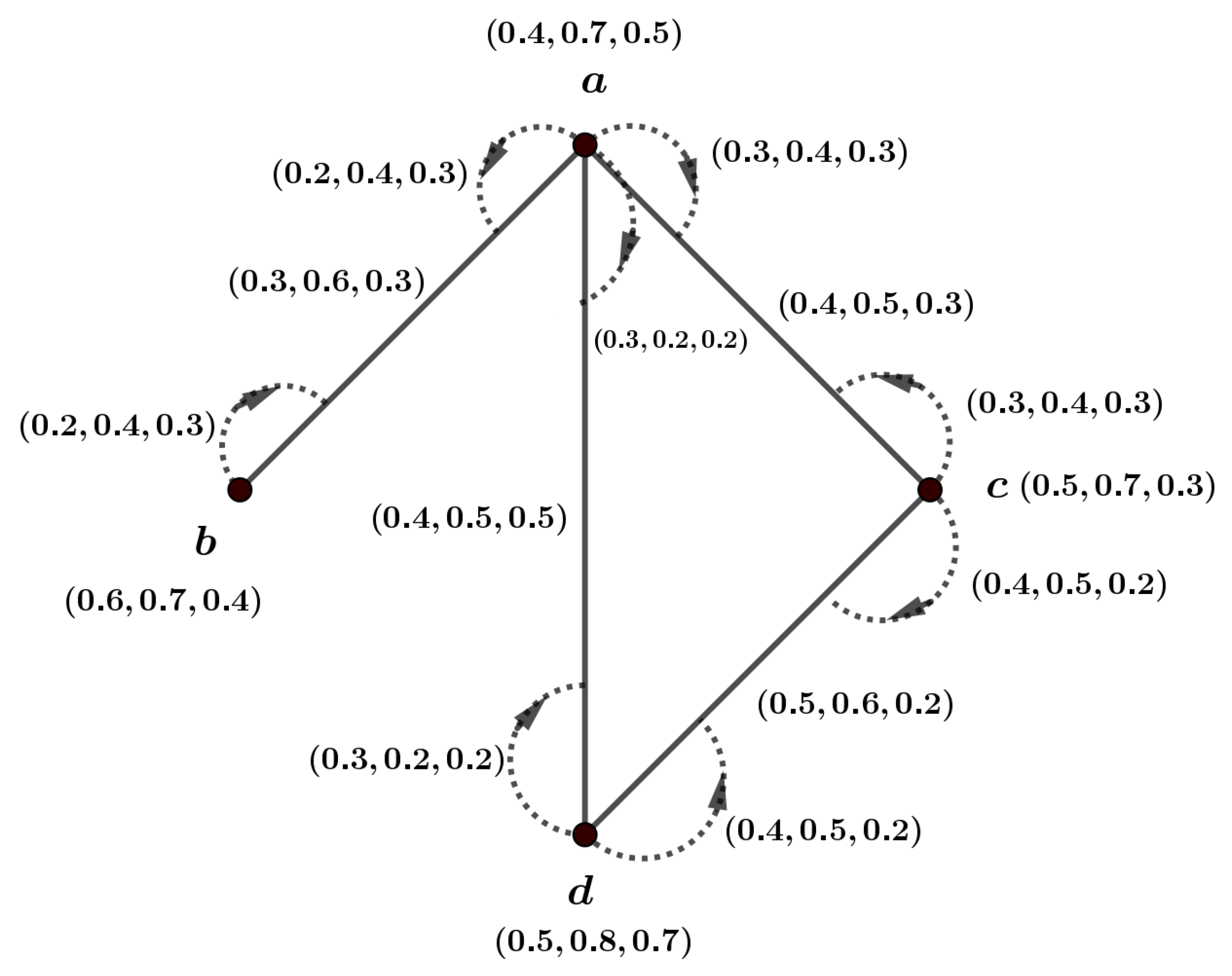
Definition 18. 

An m-dimensional PFIG $\tilde{G}=(W,\tau ,\nu ,\psi )$ is called a complete m-PFIG if for every vertex $b_1\in W$ and for every edge $(b_1,b_2)\in F$, the condition $p_i\circ \psi (b_1,(b_1,b_2))=min\{p_i\circ \tau \left(b_1\right),p_i\circ \nu (b_1,b_2)\}$ holds for each $i=1,2,\dots ,n$. An m-dimensional PFIG $\tilde{G}=(W,\tau ,\nu ,\psi )$ is considered strong if for every edge $(b_1,(b_1,b_2))\in \psi$, the condition $p_i\circ \psi (b_1,(b_1,b_2))=min\{p_i\circ \tau \left(b_1\right),p_i\circ \nu (b_1,b_2)\}$ is satisfied for all $i=1,2,\dots ,m$. If $\tilde{G}=(W,\tau ,\nu ,\psi )$ is a complete m-PFIG and the vertices $b_1$ and $b_2$ are adjacent at the edge $(b_1,b_2)$, then the following holds: $p_i\circ \psi (b_1,(b_1,b_2))=min\{p_i\circ \tau \left(b_1\right),p_i\circ \nu (b_1,b_2)\}=min\{p_i\circ \tau \left(b_2\right),p_i\circ \nu (b_1,b_2)\}=p_i\circ \psi (b_2,(b_1,b_2))$ for all $i=1,2,\dots ,m$. Figure 2 describes an example.

Figure 2. Example of a Strong and Complete m-PFIG $\tilde{G}$.

Theorem 1. 

A complete m-PFIG is also classified as a strong m-PFIG.

Proof. 

Let $\tilde{G}=(W,\tau ,\nu ,\psi )$ be a complete m-PFIG, and consider $(b_1,(b_1,b_2))$ as a pair in $\tilde{G}$. For all $b_1\in W$ and $(b_1,b_2)\in F$, it follows that $p_i\circ \psi (b_1,(b_1,b_2))=min\{p_i\circ \tau \left(b_1\right),p_i\circ \nu (b_1,b_2)\}$ for each $i=1,2,\dots ,m$. Consequently, this implies that $p_i\circ \psi (b_1,(b_1,b_2))=min\{p_i\circ \tau \left(b_1\right),p_i\circ \nu (b_1,b_2)\}$ holds for all pairs $(b_1,(b_1,b_2))$ in $\psi$ and for each $i=1,2,\dots ,m$. Therefore, $\tilde{G}$ qualifies as a strong m-PFIG. □

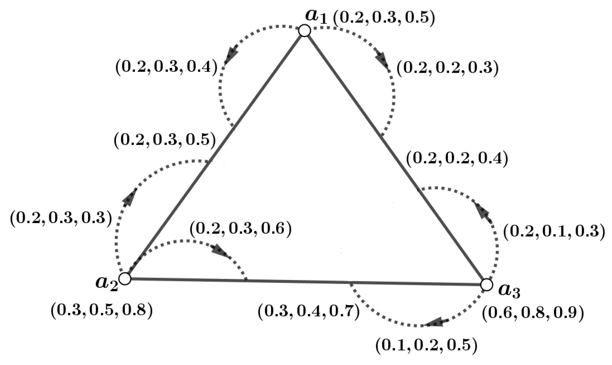
Definition 19. 

Let $x=x_1,x_2,\dots ,x_{n-1}=y$ and $x_n=z$ represent the n vertices in an m-dimensional PFIG $\tilde{G}$. An incidence path in $\tilde{G}$ can be described as follows: $x_1,(x_1,(x_1,x_2)),(x_1,x_2),(x_2,(x_1,x_2)),x_2,\dots ,y,(y,(y,z)),(y,z),\dots ,z,(z,(y,z)).$ The IS of this path is denoted as $p_i\circ {\psi }_{x,(y,z)}$ and is represented by the expression: $p_i\circ {\psi }_{x,(y,z)}=p_i\circ \psi (x_1,(x_1,x_2))\wedge p_i\circ \psi (x_2,(x_1,x_2))\wedge \cdots \wedge p_i\circ \psi (y,(y,z))\wedge p_i\circ \psi (z,(y,z)).$ The ISC between x and $(y,z)$ in $\tilde{G}$ is represented as $ICON{N}_{\tilde{G}}(x,(y,z))$, given by the following expression:

$$ICON{N}_{\tilde{G}}(x,(y,z))=\vee (\mathit{incidence}\mathit{strengths}\mathit{of}\mathit{all}\mathit{the}\mathit{paths}\mathit{connecting}x\mathit{and}(y,z)).$$

Example 1. 

Consider the connected m-PFIG illustrated in Figure 3. Here, $p_i\circ {\psi }_{a_1,(a_2,a_3)}$ $=p_i\circ {\psi }_{a_1,(a_1,a_2)}$ $\wedge p_i\circ {\psi }_{a_2,(a_1,a_2)}\wedge p_i\circ {\psi }_{a_2,(a_2,a_3)}\wedge p_i\circ {\psi }_{a_3,(a_2,a_3)}$. Now, we have, for $i=1,p_i\circ {\psi }_{a_1,(a_1,a_2)}\wedge p_i\circ {\psi }_{a_2,(a_1,a_2)}\wedge p_i\circ {\psi }_{a_2,(a_2,a_3)}=0.2$, $i=2,p_i\circ {\psi }_{a_1,(a_1,a_2)}\wedge p_i\circ {\psi }_{a_2,(a_1,a_2)}\wedge p_i\circ {\psi }_{a_2,(a_2,a_3)}=0.3$, $i=3,p_i\circ {\psi }_{a_1,(a_1,a_2)}\wedge p_i\circ {\psi }_{a_2,(a_1,a_2)}\wedge p_i\circ {\psi }_{a_2,(a_2,a_3)}=0.3$. In general, $p_i\circ {\psi }_{a_1,(a_1,a_2)}\wedge p_i\circ {\psi }_{a_2,(a_1,a_2)}\wedge p_i\circ {\psi }_{a_2,(a_2,a_3)}=(0.2,0.3,0.3)$, $p_i\circ {\psi }_{a_1,(a_1,a_3)}\wedge p_i\circ {\psi }_{a_3,(a_1,a_3)}\wedge p_i\circ {\psi }_{a_3,(a_2,a_3)}=(0.1,0.1,0.3).$ $ICON{N}_{\tilde{G}}(a_1,(a_2,a_3))=\vee \{(0.2,0.3,0.3),(0.1,0.1,0.3)\}=(0.2,0.3,0.3)$.

Figure 3. An illustrative example of an m-PFIG $\tilde{G}$, showing the connections among vertices, edges, and their corresponding incidence membership values.

Definition 20. 

Let $(y_1,y_2)$ denote an edge in an m-dimensional PFIG $\tilde{G}=(W,\tau ,\nu ,\psi )$. If $p_i\circ \psi (y_1,(y_1,y_2))>0$ and $p_i\circ \psi (y_2,(y_1,y_2))>0$, then the pairs $(y_1,(y_1,y_2))$ and $(y_2,(y_1,y_2))$ are considered pairs. The graph $\tilde{G}$ is said to be connected if there exists an incidence path that connects every pair of vertices.

Theorem 2. 

Let $\tilde{G}=(W,\tau ,\nu ,\psi )$ be an m-dimensional PFIG, and let $\widetilde{G_1}=(W_1,{\tau }_1,{\nu }_1,{\psi }_1)$ be an m-dimensional PFIS of $\tilde{G}$. For any pair $(r_1,(r_1,r_2))$ in $\tilde{G}$ and $\widetilde{G_1}$, it holds that

$$p_i\circ ICON{N}_{\tilde{G}}(r_1,(r_1,r_2))\ge p_i\circ ICON{N}_{{\tilde{G}}_1}(r_1,(r_1,r_2)).\forall i=1,2,\dots ,m.$$

Proof. 

Consider $\widetilde{G_1}$ as a subgraph of the m-dimensional PFIG $\tilde{G}$. According to the definition of an m-dimensional PFIS, we have $p_i\circ {\psi }_1(r_1,(r_1,r_2))=p_i\circ \psi (r_1,(r_1,r_2))$ for every pair $(r_1,(r_1,r_2))$ in ${\psi }_1,\forall i=1,2,\dots ,m$. The terms $ICON{N}_{\tilde{G}}(r_1,(r_1,r_2))$ and $ICON{N}_{{\tilde{G}}_1}(r_1,(r_1,r_2))$ may correspond to the same incidence pair in both $\widetilde{G_1}$ and $\tilde{G}$; otherwise, they may refer to different pairs in these graphs. This situation leads us to consider two distinct cases. □

Case 1. 

Assume that $ICON{N}_{\tilde{G}}(r_1,(r_1,r_2))$ and $ICON{N}_{{\tilde{G}}_1}(r_1,(r_1,r_2))$ are associated with the same pair $(s_1,(s_1,s_2))$ in both $\widetilde{G_1}$ and $\tilde{G}$. Based on the definition of an m-dimensional PFIS, we have $p_i\circ {\psi }_1(s_1,(s_1,s_2))=p_i\circ \psi (s_1,(s_1,s_2)),\forall i=1,2,\dots ,m$. Consequently, it follows that

$$p_i\circ ICON{N}_{\tilde{G}}(r_1,(r_1,r_2))=p_i\circ ICON{N}_{{\tilde{G}}_1}(r_1,(r_1,r_2)).$$

Case 2. 

Let us consider that $ICON{N}_{\tilde{G}}(r_1,(r_1,r_2))$ and $ICON{N}_{{\tilde{G}}_1}(r_1,(r_1,r_2))$ correspond to the pairs $(s_1^{\prime },(s_1^{\prime },s_2^{\prime }))$ in $\tilde{G}$ and $(s_3^{\prime },(s_3^{\prime },s_4^{\prime }))$ in $\widetilde{G_1}$. This indicates that both pairs $(s_1^{\prime },(s_1^{\prime },s_2^{\prime }))$ and $(s_3^{\prime },(s_3^{\prime },s_4^{\prime }))$ exist within $\tilde{G}$. If $p_i\circ \psi (s_1^{\prime },(s_1^{\prime },s_2^{\prime }))=p_i\circ \psi (s_3^{\prime },(s_3^{\prime },s_4^{\prime }))$, it follows that

$$p_i\circ ICON{N}_{\tilde{G}}(r_1,(r_1,r_2))=p_i\circ ICON{N}_{{\tilde{G}}_1}(r_1,(r_1,r_2)).$$

Again, if $p_i\circ \psi (s_1^{\prime },(s_1^{\prime },s_2^{\prime }))\ne p_i\circ \psi (s_3^{\prime },(s_3^{\prime },s_4^{\prime }))$, then it leads to $p_i\circ ICON{N}_{\tilde{G}}(r_1,(r_1,r_2))\ne p_i\circ ICON{N}_{{\tilde{G}}_1}(r_1,(r_1,r_2))$, meaning that either $p_i\circ ICON{N}_{\tilde{G}}(r_1,(r_1,r_2))>p_i\circ ICON{N}_{{\tilde{G}}_1}$$(r_1,(r_1,r_2))$ or $p_i\circ ICON{N}_G(r_1,(r_1,r_2))<p_i\circ ICON{N}_{G_1}(r_1,(r_1,r_2)).$ But, we cannot accept $p_i\circ ICON{N}_G(r_1,(r_1,r_2))<p_i\circ ICON{N}_{G_1}(r_1,(r_1,r_2))$ because it violates the fundamental property of fuzzy subgraph mappings. Therefore, in all situations, $p_i\circ ICON{N}_{\tilde{G}}(r_1,(r_1,r_2))\ge p_i\circ ICON{N}_{{\tilde{G}}_1}(r_1,(r_1,r_2)).$

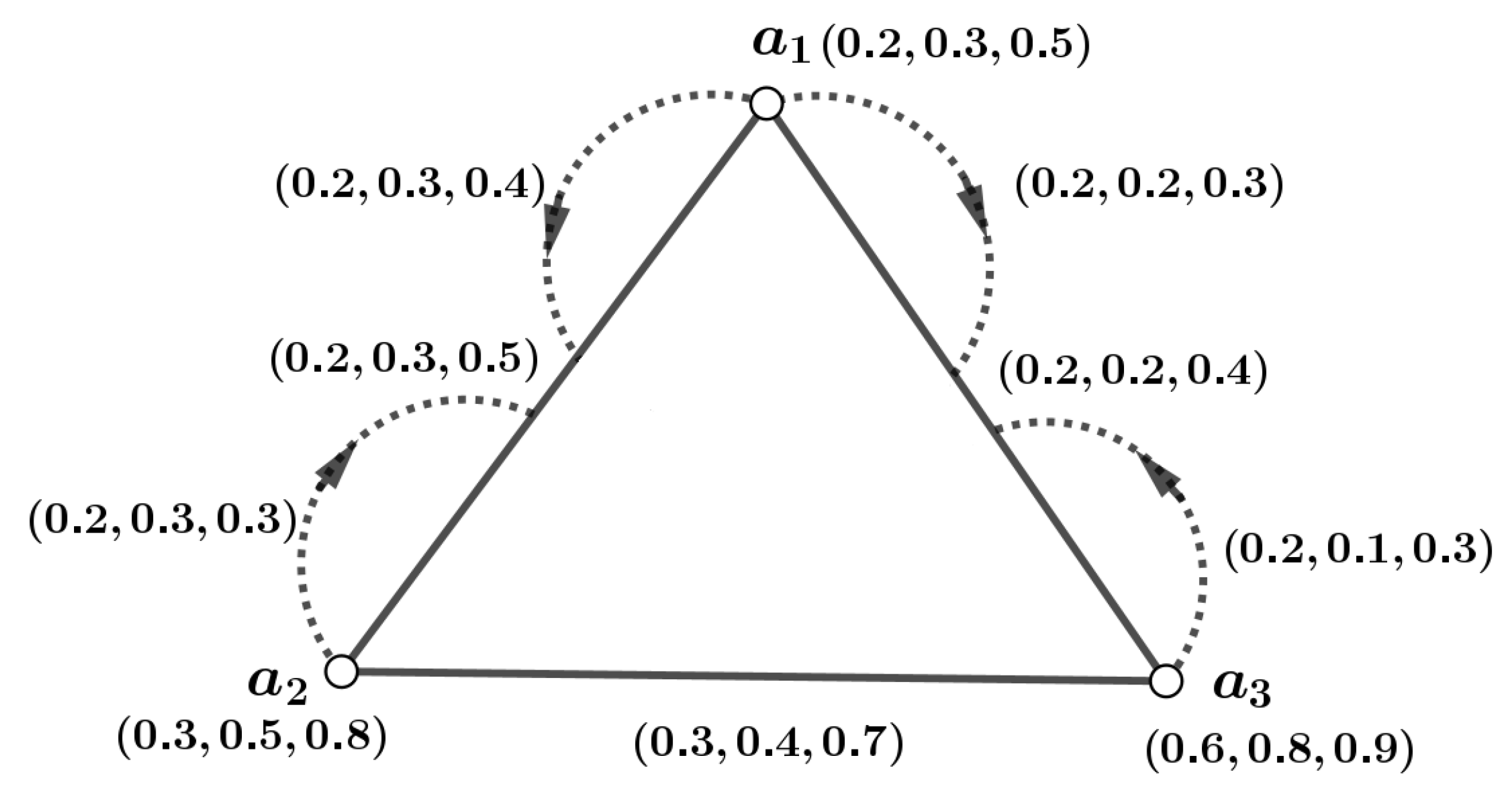
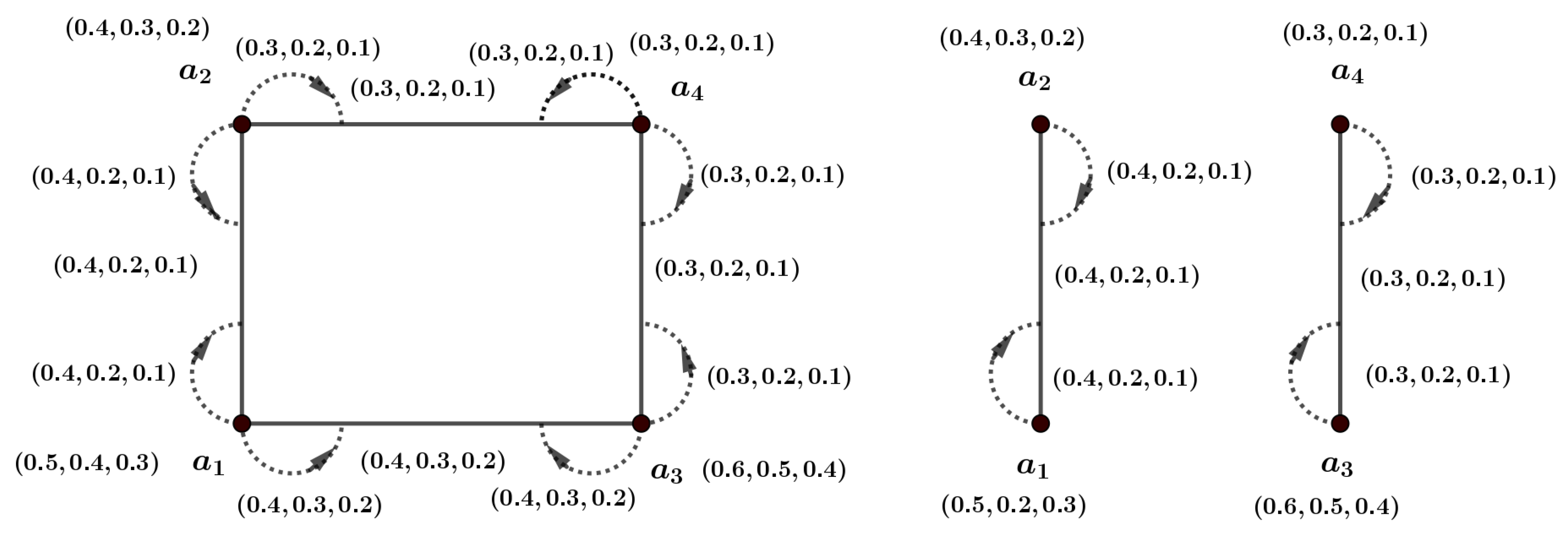
Example 2. 

In Figure 4 we consider $\tilde{H}$ as the m-PFIS of the graph $\tilde{G}$ of Figure 3. Now, $ICON{N}_{\tilde{G}}(a_1,(a_1,a_2))=(0.2,0.3,0.3)$ and $ICON{N}_{\tilde{H}}(a_1,(a_1,a_2))=(0.2,0.3,0.3)$. Therefore, $p_i\circ ICON{N}_{\tilde{G}}(a_1,(a_1,a_2))=p_i\circ ICON{N}_{\tilde{H}}(a_1,(a_1,a_2)),\forall i=1,2,3.$

Figure 4. An m-PFIS $\tilde{H}$ of the m-FIG $\tilde{G}$ of Figure 3.

Definition 21. 

A pair $(a_1,a_2)$ in $\tilde{G}=(W,\tau ,\nu ,\psi )$ is considered a strong pair if $p_i\circ \psi (a_1,(a_1,a_2))\ge p_i\circ ICON{N}_{\tilde{G}}(a_1,(a_1,a_2)),\forall i=1,2,3,\dots ,m.$.

Example 3. 

From the m-PFIG $\tilde{G}$ of Figure 5 we have, $p_i\circ \psi (a_1,(a_1,a_2))=(0.2,0.3,0.4)$, $p_i\circ \psi (a_2,(a_2,a_3))=(0.2,0.3,0.6)$, $p_i\circ ICON{N}_{\tilde{G}}(a_1,(a_1,a_2))$$=(0.2,0.3,0.3)$, $p_i\circ ICON{N}_{\tilde{G}}(a_2,(a_2,a_3))$$=(0.2,0.3,0.6)$, $p_i\circ ICON{N}_{\tilde{G}}(a_1,(a_1,a_2))>p_i\circ \psi (a_1,(a_1,a_2))$, $p_i\circ ICON{N}_{\tilde{G}}(a_2,(a_2,a_3))=p_i\circ \psi (a_2,(a_2,a_3))$, $\forall i=1,2,3.$ $\therefore (a_1,(a_1,a_2))$ is not strong pair but $(a_2,(a_2,a_3))$ is a strong pair.

Figure 5. An example of m-PFIG $\tilde{G}$.

Theorem 3. 

In a complete m-PFIG, every edge forms a strong pair.

Proof. 

Consider $\tilde{G}=(W,\tau ,\nu ,\psi )$ as an m-PFIG, and consider the pair $(a_1,(a_1,a_2))$ in $\psi$. We have $p_i\circ \psi (a_1,(a_1,a_2))=\wedge \{p_i\circ \tau \left(a_1\right),p_i\circ \nu (a_1,a_2)\}$. According to the previous theorem, this establishes that $(a_1,(a_1,a_2))$ is identified as a strong pair in $\tilde{G}$. Since $(a_1,(a_1,a_2))$ is chosen arbitrarily from the complete m-PFIG $\tilde{G}$, it can be inferred that every pair in $\tilde{G}$ qualifies as a strong pair. □

Definition 22. 

Let $\tilde{G}=(W,\tau ,\nu ,\psi )$ denote an m-PFIG, and let $\tilde{H}=(V_1,{\tau }_1,{\nu }_1,{\psi }_1)$ represent an m-PFIS of $\tilde{G}$. This subgraph $\tilde{H}$ is defined such that for every pair $(a_1,(a_1,a_2))$ in ψ, it holds that $\tilde{H}=\tilde{G}-\left\{(a_1,(a_1,a_2))\right\}$. If $p_i\circ ICON{N}_{\tilde{G}}(x_1,(x_1,x_2))>p_i\circ ICON{N}_{\tilde{H}}(x_1,(x_1,x_2))$ for a particular pair $(x_1,(x_1,x_2))$ in ψ, then the pair $(a_1,(a_1,a_2))$ is referred to as an incidence cut pair of $\tilde{G}$.

4. Matching Idea on $\mathbf{m}$-PFIG

Some fundamental definitions are covered in this chapter, such as support for m-PFIGs, the degree of incidence pairs, the degree of vertices, and the degree of edges in m-PFIGs, as well as the path, strength, connectedness strength, matching, MPN, MMPN, instances, and theorems.

$\tau$, $\nu =W\times W$, and $\psi =W\times F$ represent the sets of vertices, edges, and incidence pairs, respectively, in this section. Assume that the graph $G=(W,F)$ is a crisp graph. Two edges in a graph are said to be adjacent if they share a common vertex and non-adjacent if they do not share any common vertex. A collection $\tilde{M}$ of pairwise edges that are non-adjacent is referred to as matching.

If a matching $\tilde{M}$ covers every vertex in the crisp graph G, it is referred to as a perfect matching. If a matching $\tilde{M}$ covers the highest number of vertices, it is termed a maximum matching. A crisp graph G is considered to have a nearly perfect matching if just one vertex remains unmatched. The matching number, denoted as $\beta \left(\tilde{M}\right)$, refers to the total count of edges present in the maximum matching. Edges that alternate between $\tilde{M}$ and F are referred to as a track.

Definition 23. 

If $\tilde{G}=(W,\tau ,\nu ,\psi )$ is the m-PFIG, then $\breve{G}=(W^{\ast },{\tau }^{\ast },{\nu }^{\ast },{\psi }^{\ast })$ represents the support of m-PFIG and is defined as follows:

• ${\tau }^{\ast }=\{v_x\in W:p_i\circ \tau \left(v_x\right)>0\}$, $\forall i=1,2,3,\dots ,m.$
• ${\nu }^{\ast }=\{(v_x,v_y)\in W\times W:p_i\circ \nu (v_x,v_y)>0\}$, $\forall i=1,2,3,\dots ,m.$
• ${\psi }^{\ast }=\{(v_x,(v_x,v_y))\in W\times E:p_i\circ \psi (v_x,(v_x,v_y))>0\}$, $\forall i=1,2,3,\dots ,m.$

Definition 24. 

Let the m-PFIG be $\tilde{G}=(W,\tau ,\nu ,\psi )$. If there is a path from $v_x$ to $v_y$ such that $v_x,(v_x,(v_x,v_y),(v_x,v_y),(v_y,\left(v_x{v}_y\right)),v_y$, then two vertices $v_x$ and $v_y$ are said to be connected. An edge $(v_x,v_y)$ and a vertex $v_x$ are considered connected if there is a path connecting them that appears to be the following: $v_x,(v_x,(v_x,v_y)),(v_x,v_y).$

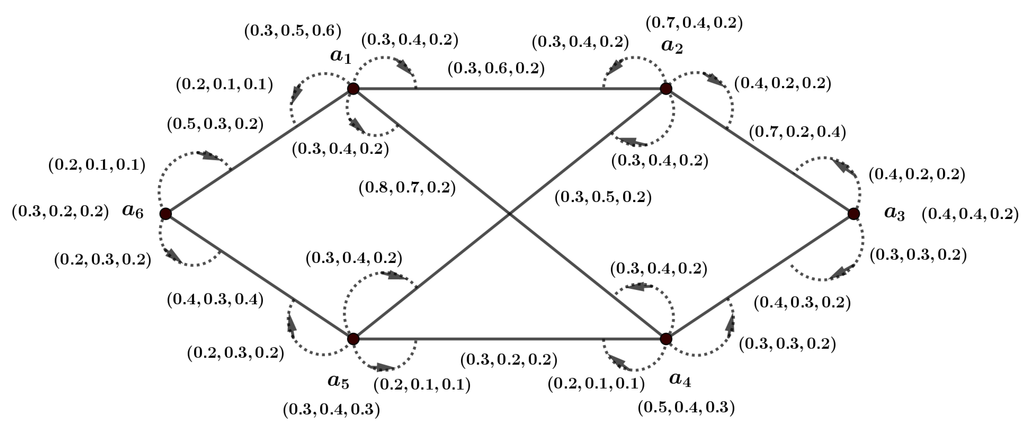
Definition 25. 

Assume that the m-PFIG is $\breve{G}=(W^{\ast },{\tau }^{\ast },{\nu }^{\ast },{\psi }^{\ast })$. Subsequently, $\forall i=1,2,3,\dots ,m$, any vertex $v_x\in {\tau }^{\ast }$ in $\breve{G}$ has the degree defined as follows:

$$p_i\circ deg\left(v_x\right)=\sum _{v_y\in {\tau }^{\ast },v_x\ne v_y}{p}_i\circ \psi (v_x,(v_x,v_y)).$$

In $\breve{G}$, the degree of an edge $\nu (v_x,v_y)\in {\nu }^{\ast }$, where $v_x\ne v_y$ and $i=1,2,3,\dots ,m$, is as follows:

$$p_i\circ deg(v_x,v_y)=\sum _{v_z\in {\tau }^{\ast },v_x\ne v_z}{p}_i\circ \nu (v_x,v_z)+\sum _{v_z\in {\tau }^{\ast },v_y\ne v_z}{p}_i\circ \nu (v_y,v_z)-2(p_i\circ \nu (v_x,v_y)).$$

In $\tilde{G}$, the degree of any incidence pair $\psi (v_x,(v_x,v_y))\in {\psi }^{\ast }$ where $v_x\ne v_y$ and $i=1,2,3,\dots ,m$ is defined as follows:

$$p_i\circ deg(v_x,(v_x,v_y))=\sum _{v_z\in {\tau }^{\ast },v_x\ne v_z}{p}_i\circ \psi (v_x,(v_x,v_z))+\sum _{v_z\in {\tau }^{\ast },v_y\ne v_z}{p}_i\circ \psi (v_y,(v_y,v_z))-2(p_i\circ \psi (v_x,(v_x,v_y))).$$

Example 4. 

The m-PFIG depicted in Figure 6 is examined. The degree of incidence pairs, edges, and vertices will also be calculated. The following is the degree of distinct vertices: $p_i\circ deg\left(a\right)=(0.8,1.0,0.8)$, $p_i\circ deg\left(b\right)=(0.2,0.4,0.3)$, $p_i\circ deg\left(c\right)=(0.7,0.9,0.5)$, $p_i\circ deg\left(d\right)=(0.7,0.7,0.4)$. The degree of the edges is given as follows: $p_i\circ deg(a,b)=(0.8,0.1,0.8)$, $p_i\circ deg(a,d)=(1.2,1.7,0.8)$, $p_i\circ deg(a,c)=(1.2,1.7,1)$, $p_i\circ deg(c,d)=(0.8,1,0.8)$. Likewise, the degree of different pairs of incidence are provided as follows: $p_i\circ deg(a,(a,b))=(0.8,0.1,0.8),$ $p_i\circ deg(c,(c,d))=(1,1.1,0.7),$ $p_i\circ deg(d,(a,d))=(1.2,1.5,1)$ $p_i\circ deg(a,(a,c))=(0.9,1.3,0.8).$

Figure 6. An m-PFIG.

Definition 26. 

${\mathit{CONN}}_{\tilde{G}}\psi (v_x,(v_x,v_y)),$ represents the strength of connectedness between $v_x,v_y\in W\left(\tilde{G}\right)$ in the m-PFIG, where ${\mathit{CONN}}_{\tilde{G}}\psi (v_x,(v_x,v_y))$ is the highest strength of each path between $v_x$ and $v_y$, respectively.

In this study, $S\left(P\right)$ represents the strength of a path, and ${\psi }^{\infty }(v_x,(v_x,v_y))$ represents the strength of connectedness ${\mathit{CONN}}_{\tilde{G}}\psi (v_x,(v_x,v_y))$. It is equivalent to $\tilde{M}$ to have the set of vertices, edges, and incidence pair $\tau \left(\tilde{M}\right)$, $\nu \left(\tilde{M}\right)$, and $\psi \left(\tilde{M}\right)$, where $\tilde{M}$ is a matching of $\breve{G}=(W^{\ast },{\tau }^{\ast },{\nu }^{\ast },{\psi }^{\ast })$. The notation $\tilde{M}\left(\breve{G}\right)$ indicates the set that contains all matchings within $\breve{G}$. If W is equivalent to $W\left(\tilde{M}\right)$, then $\breve{G}$ is a covering matching.

Definition 27. 

Consider the m-PFIG represented as $\breve{G}=(W^{\ast },{\tau }^{\ast },{\nu }^{\ast },I^{\ast })$, with a subgraph denoted as $\breve{H}=(W_1^{\ast },{\tau }_1^{\ast },{\nu }_1^{\ast },I_1^{\ast })$. This subgraph is defined as a matching in $\breve{G}$ if, for every $u\in W^{\ast }$, there exists exactly one $v\in W_1^{\ast }$ such that $v\ne u$ and $p_i\circ {\nu }_{\tilde{M}}(u,v)\ge 0$.

Example 5. 

Observe an m-PFIG with a single possible matching, as shown in Figure 7. In this m-PFIG, we have: $\tau \left(\tilde{M}\right)=\{a_1,a_2,a_3,a_4\}$, $\nu \left(\tilde{M}\right)=\{(a_1,a_2),(a_3,a_4)\}$, and $\psi \left(\tilde{M}\right)=\{(a_1,(a_1,a_2)),(a_3,(a_3,a_4))\}$.

Figure 7. An m-PFIG $\tilde{G}$ with possible matching $\tilde{M}$.

Corollary 1. 

Let us consider the m-PFIG represented by $\breve{G}=(W^{\ast },{\tau }^{\ast },{\nu }^{\ast },{\psi }^{\ast })$. A matching in $\breve{G}$ induces any matching in $\tilde{G}$.

Proof. 

Since a set of triples like $⟨\dots ,v_x{e}_j{v}_z,\dots ⟩$ is considered a matching, we need to clearly indicate the vertices and incidence pair. Thus, as seen in Figure 7, a matching M can be expressed as $⟨(a_1,(a_1,a_2)),(a_3,(a_3,a_4))⟩$. □

Proposition 1. 

Let $\breve{G}=(W^{\ast },{\tau }^{\ast },{\nu }^{\ast },{\psi }^{\ast })$ be the m-PFIG. Assuming that $\tilde{M}$ corresponds to $\breve{G}$, then ${\psi }^{\infty }(v_x,(v_x,v_y))=p_i\circ \psi (v_x,(v_x,v_y))$, for all $v_x,v_y\in \tau \left(\tilde{M}\right)$.

Proof. 

Let $v_x,v_y\in \tau \left(\tilde{M}\right)$. A path that connects $v_x$ and $v_y$ is equivalent to a single incidence pair $(v_x,(v_x,v_y))$ and $S\left(P\right)=p_i\circ \psi (v_x,(v_x,v_y))$; otherwise, we have $S\left(P\right)=p_i\circ \psi (v_x,(v_x,v_y))=0$. Therefore, ${\psi }^{\infty }(v_x,(v_x,v_y))(p_i\circ \psi (v_x,(v_x,v_y)))=p_i\circ \psi (v_x,(v_x,v_y))$ for each case. □

Theorem 4. 

Let us consider the m-PFIG represented by $\breve{G}=(W^{\ast },{\tau }^{\ast },{\nu }^{\ast },{\psi }^{\ast })$ containing a matching $\tilde{M}$. Then, $p_i\circ \mathrm{deg}\left(v_x\right)=p_i\circ \mathrm{deg}\left(v_y\right)=p_i\circ (v_x,(v_x,v_y))$ and $p_i\circ \mathrm{deg}(v_x,(v_x,v_y))=0$ for every $(v_x,v_y)\in \tilde{M}$ and $\forall i=1,2,3,\dots ,m$.

Proof. 

As for every $v_x\in \tau \left(\tilde{M}\right)$, there is only one $v_y\in \tau \left(\tilde{M}\right)$ such that $p_i\circ \psi (v_x,(v_x,v_y))>0$ $\forall i=1,2,3,\dots ,m$; we get: $p_i\circ \mathrm{deg}\left(v_x\right)={\sum }_{v_z\in \tau \left(\tilde{M}\right),v_z\ne v_x}{p}_i\circ \psi (v_x,(v_x,v_z))={\sum }_{v_z=v_y}{p}_i\circ \psi (v_x,(v_x,v_y))=p_i\circ \psi (v_x,(v_x,v_y)),$ and $p_i\circ \mathrm{deg}(v_x,(v_x,v_y))={\sum }_{v_z\in \tau \left(\tilde{M}\right)}{p}_i\circ \psi (v_x,(v_x,v_z))$$+{\sum }_{v_z\in \tau \left(\tilde{M}\right)}{p}_i\circ \psi (v_y,(v_y,v_z))$$-2(p_i\circ \psi (v_x,(v_x,v_y)))$$p_i\circ \mathrm{deg}(v_x,(v_x,v_y))={\sum }_{v_z=v_y}{p}_i\circ$$\psi (v_x,(v_x,v_z))+{\sum }_{v_z=v_x}{p}_i\circ \psi (v_y,(v_y,v_z))$ − $2(p_i\circ \psi (v_x,(v_x,v_y)))$ $p_i\circ \mathrm{deg}\psi (v_x,(v_x,v_y))=p_i\circ \psi (v_x,(v_x,v_y))+p_i\circ \psi (v_y,(v_y,v_x))$ − $2(p_i\circ \psi (v_x,(v_x,v_y)))$ = 0. □

Definition 28. 

In m-PFIG $\breve{G}=(W^{\ast },{\tau }^{\ast },{\nu }^{\ast },I^{\ast })$, let $\tilde{M}$ be a matching. subsequently:

(i) 

The corresponding m-PFIN of $\tilde{M}$ can be explained as follows:

$$p_i\circ {\beta }_{\psi }\left(\tilde{M}\right)=\sum _{\psi \in \psi \left(\tilde{M}\right)}{p}_i\circ \psi (v_x,(v_x,v_y)),\forall i=1,2,3,\dots ,m.$$

(ii) 

The definition of the matching edge m-PFIN of $\tilde{M}$ is as follows:

$$p_i\circ {\beta }_{\nu }\left(\tilde{M}\right)=\sum _{e\in \nu \left(\tilde{M}\right)}{p}_i\circ \nu (v_x,v_y),\forall i=1,2,3,\dots ,m.$$

(iii) 

The corresponding vertex m-PFIN of $\tilde{M}$ can be explained as follows:

$$p_i\circ {\beta }_{\tau }\left(\tilde{M}\right)=\sum _{v_x\in \tau \left(\tilde{M}\right)}{p}_i\circ \tau \left(v_x\right),\forall i=1,2,3,\dots ,m.$$

(iv) 

The corresponding crisp number of $\tilde{M}$ can be explained as follows:

$$p_i\circ {\beta }_C\left(\tilde{M}\right)=\left|\tilde{M}\right|,\forall i=1,2,3,\dots ,m.$$

The crisp number in a matching for an m-PFIG is the cardinality (count) of the matching set, i.e., the number of distinct, non-overlapping edges selected in the matching, ignoring the m-polar membership values. Even though each edge has multiple fuzzy components, the crisp number only reflects how many matches exist.

The terms $p_i\circ {\beta }_{\psi }\left(\tilde{M}\right)$, $p_i\circ {\beta }_{\tau }\left(\tilde{M}\right)$, and $p_i\circ {\beta }_C\left(\tilde{M}\right)$ are regarded as the Matching m-Polar Fuzzy Incidence Principal Numbers (MmPFIPNs) associated with $\tilde{M}$.

Example 6. 

Figure 7 shows an m-PFIG with a possible matching. MBFIPNs can be obtained as $p_i\circ {\beta }_{\psi }\left(\tilde{M}\right)=(0.7,0.4,0.2)$, $p_i\circ {\beta }_{\tau }\left(\tilde{M}\right)=(1.8,1.2,1)$, and $p_i\circ {\beta }_C\left(\tilde{M}\right)=2$.

Definition 29. 

In an m-PFIG $\breve{G}=(W^{\ast },{\tau }^{\ast },{\nu }^{\ast },I^{\ast })$, let $\tilde{M}$ be a matching. Then:

(i) 

It is possible to describe the MMm-PFIN of $\breve{G}$ as follows:

$$p_i\circ {\beta }_{\psi }^{\max }\left(\tilde{M}\right)=max\{{\beta }_{\psi }\left(\tilde{M}\right):\tilde{M}\in \tilde{M}\left(\breve{G}\right\}.$$

(ii) 

The corresponding MMEm-PFIN of $\breve{G}$ can be obtained as follows:

$$p_i\circ {\beta }_{\nu }^{\max }\left(\tilde{M}\right)=max\{{\beta }_{\nu }\left(\tilde{M}\right):\tilde{M}\in \tilde{M}\left(\breve{G}\right\}.$$

(iii) 

The corresponding MMVm-PFIN of $\breve{G}$ can be defined as follows:

$$p_i\circ {\beta }_{\tau }^{\max }\left(\tilde{M}\right)=max\{{\beta }_{\tau }\left(\tilde{M}\right):\tilde{M}\in \tilde{M}\left(\breve{G}\right\}.$$

(iv) 

The following defines the MMCN of $\breve{G}$:

$$p_i\circ {\beta }_C^{\max }\left(\tilde{M}\right)=max\{{\beta }_C\left(\tilde{M}\right):\tilde{M}\in \tilde{M}\left(\breve{G}\right)\}.$$

$p_i\circ {\beta }_{\psi }^{\max }\left(\tilde{M}\right)$, $p_i\circ {\beta }_{\tau }^{\max }\left(\tilde{M}\right)$, and $p_i\circ {\beta }_C^{\max }\left(\tilde{M}\right)$ are regarded as MMm-PFIN, MMVm-PFIN, and MMCN, respectively. There are several matchings with the same MMCN in classical graph theory. We can differentiate them using fuzzy values in the fuzzy sense.

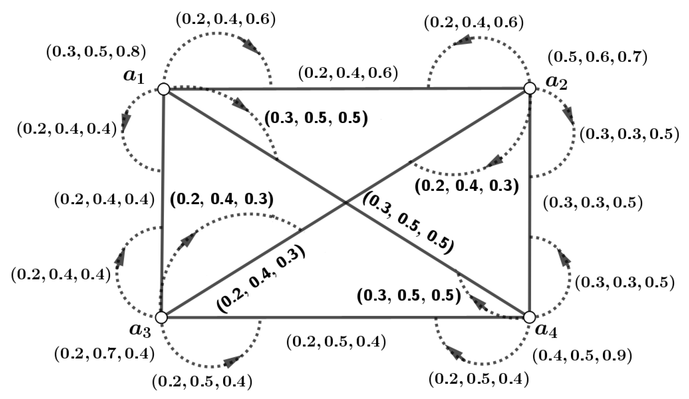
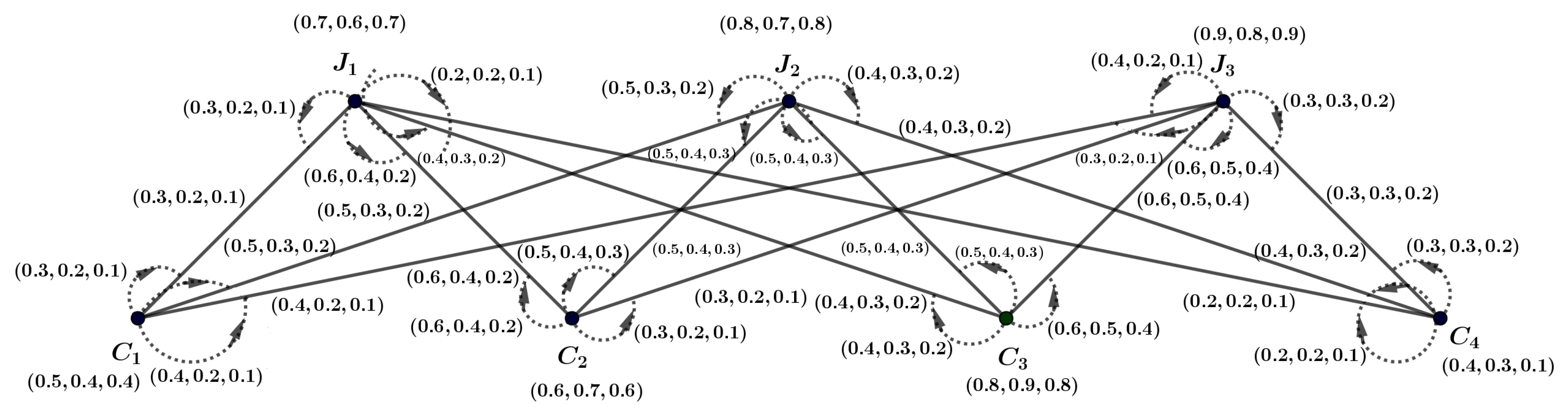
Example 7. 

Figure 8 shows an mPFIG $\breve{G}=(W^{\ast },{\tau }^{\ast },{\nu }^{\ast },{\psi }^{\ast })$. We will now determine all possible matchings—MmPFIPNs, MMmPFIN, MMVmPFIN, and MMCN—for Figure 8, as shown in Table 2.

Figure 8. An m-PFIG $\tilde{G}$.

Table 2. All possible matchings and MmPFIPNs of m-PFIG for Figure 8.

Matching Possibilities	${\mathit{\beta }}_{\mathit{\psi }}\left(\tilde{\mathit{M}}\right)$	${\mathit{\beta }}_{\mathit{\tau }}\left(\tilde{\mathit{M}}\right)$	${\mathit{\beta }}_{\mathit{C}}\left(\tilde{\mathit{M}}\right)$
$\{\psi (a_1,(a_1,a_2)),\psi (a_5,(a_5,a_4))\}$	$(0.5,0.5,0.3)$	$(1.8,1.7,1.4)$	2
$\{\psi (a_1,(a_1,a_6)),\psi (a_2,(a_2,a_3))\}$	$(0.6,0.3,0.3)$	$(1.7,1.5,1.2)$	2
$\{\psi (a_1,(a_1,a_4)),\psi (a_2,(a_2,a_5))\}$	$(0.6,0.8,0.4)$	$(1.8,1.7,1.4)$	2
$\{\psi (a_2,(a_2,a_3)),\psi (a_5,(a_5,a_6))\}$	$(0.6,0.5,0.4)$	$(1.7,1.4,0.7)$	2
$\{\psi (a_2,(a_2,a_5)),\psi (a_1,(a_1,a_6))\}$	$(0.5,0.5,0.3)$	$(1.6,1.5,1.3)$	2
$\{\psi (a_2,(a_2,a_5)),\psi (a_3,(a_3,a_4))\}$	$(0.6,0.7,0.4)$	$(1.9,1.6,1)$	2
$\{\psi (a_1,(a_1,a_6)),\psi (a_3,(a_3,a_4))\}$	$(0.5,0.4,0.3)$	$(1.5,1.5,1.3)$	2
$\{\psi (a_5,(a_5,a_6)),\psi (a_3,(a_3,a_4))\}$	$(0.5,0.6,0.4)$	$(1.5,1.3,1)$	2
$\{\psi (a_1,(a_1,a_2)),\psi (a_5,(a_5,a_6)),\psi (a_3,(a_3,a_4))\}$	$(0.8,0.4,0.4)$	$(2.5,2.3,1.8)$	3
$\{\psi (a_5,(a_5,a_4)),\psi (a_2,(a_2,a_3)),\psi (a_1,(a_1,a_6))\}$	$(0.8,1,0.6)$	$(2.5,2.2,1.8)$	3

As a result, calculating the following figures is straightforward: $p_i\circ {\beta }_{\psi }^{\max }\left(\tilde{M}\right)=(0.8,1,0.6)$, $p_i\circ {\beta }_{\tau }^{\max }\left(\tilde{M}\right)=(2.5,2.3,1.8)$, $p_i\circ {\beta }_C^{\max }\left(\tilde{M}\right)=3.$

Proposition 2. 

In m-PFIG $\breve{G}=(W^{\ast },{\tau }^{\ast },{\nu }^{\ast },{\psi }^{\ast })$, let $\tilde{M}$ be a matching. We therefore have the following for each $\tilde{M}\in \tilde{M}\left(\breve{G}\right)$ and $\forall i=1,2,3,\dots ,m$:

$$p_i\circ {\beta }_{\psi }\left(M\right)<p_i\circ {\beta }_{\nu }\left(M\right)<p_i\circ {\beta }_{\tau }\left(\tilde{M}\right).$$

Proof. 

Let $\tilde{M}\in \tilde{M}\left(\breve{G}\right)$. As $\tilde{M}\left(\breve{G}\right)$ is an m-PFIG, $p_i\circ \psi (v_x,(v_x,v_y))\le p_i\circ \tau \left(v_x\right)\wedge p_i\circ \nu (v_x,v_y)$ and $p_i\circ \nu (v_x,v_y)\le p_i\circ \tau \left(v_x\right)\wedge p_i\circ \tau \left(v_y\right)$ for all $\psi (v_x,(v_x,v_y))\in \tilde{M}$ and $\forall i=1,2,3,\dots ,m$. So, we have:

$$p_i\circ {\beta }_{\psi }\left(M\right)=\sum _{\psi (v_x,(v_x,v_y))\in \tilde{M}}{p}_i\circ \psi (v_x,(v_x,v_y))<\sum _{\nu (v_x,v_y)\in \nu \left(\tilde{M}\right)}{p}_i\circ \nu (v_x,v_y)<\sum _{v_x\in \tau \left(\tilde{M}\right)}{p}_i\circ \tau \left(v_x\right)=p_i\circ {\beta }_{\tau }\left(\tilde{M}\right).$$

□

Definition 30. 

With a matching $\tilde{M}$, let $\breve{G}=(W^{\ast },{\tau }^{\ast },{\nu }^{\ast },{\psi }^{\ast })$ be an m-PFIG. An $\tilde{M}$-alternating track with distinct nodes $a_1,a_2,a_3,\dots ,a_n,a_{n+1}$ is an m-polar fuzzy $\tilde{M}$-augmenting track (AT) in $\tilde{G}$. The following follows: $p_i\circ {\psi }^{\ast }(v_{i-1},(v_{i-1},v_x))>0$, where $i=1,2,3,\dots ,n,n+1$, $\{a_1,a_2,a_3,\dots ,a_n,a_{n+1}\}\subseteq p_i\circ {\tau }^{\ast }\left(\tilde{M}\right)$, Neither $a_1$ nor $a_{n+1}$ are in $p_i\circ {\tau }^{\ast }\left(\tilde{M}\right)$.

Corollary 2. 

Consider $\breve{G}=(W^{\ast },{\tau }^{\ast },{\nu }^{\ast },{\psi }^{\ast })$ as an m-PFIG that includes an $\tilde{M}$-AT P within its structure. The related crisp graph $G=(W,F)$ similarly uses P as a $\tilde{M}$-AT in this instance.

Proof. 

Let $\breve{G}=(W^{\ast },{\tau }^{\ast },{\nu }^{\ast },{\psi }^{\ast })$ be an m-polar fuzzy incidence graph (m-PFIG) associated with $\tilde{M}$. Suppose P is an m-polar fuzzy incidence $\tilde{M}$-alternating trail, and let $\Delta$ denote their symmetric difference (SD). The resulting set $P\Delta \tilde{M}$ forms a matching, as it consists of a group of incidence pairs that are mutually nonadjacent and ensures that $p_i\circ \psi (v_x,(v_x,v_y))>0$ holds for every $\psi \in P\cup \tilde{M}$. □

Theorem 5. 

Let $\breve{G}=(W^{\ast },{\tau }^{\ast },{\nu }^{\ast },{\psi }^{\ast })$ be an m-PFIG containing a matching $\tilde{M}$. If the m-PFI $\tilde{M}$-AT is P, then

$$p_i\circ {\beta }_{\tau }^{\ast }(P\Delta \tilde{M})>p_i\circ {\beta }_{\tau }^{\ast }\left(\tilde{M}\right).$$

Proof. 

An m-PF $\tilde{M}$-AT is represented by P. Definition 30 is used to obtain the following:

$$p_i\circ {\tau }^{\ast }(P\Delta \tilde{M})=p_i\circ {\tau }^{\ast }\left(\tilde{M}\right)\cup \{a_1,a_{n+1}\}.$$

We now have the following using Definition 28:

$$p_i\circ {\beta }_{\tau }^{\ast }(P\Delta \tilde{M})=\sum _{v_x\in {\tau }^{\ast }(P\Delta \tilde{M})}{p}_i\circ \tau \left(v_x\right)+p_i\circ \tau \left(v_1\right)+p_i\circ \tau \left(v_{n+1}\right).$$

$$p_i\circ {\beta }_{\tau }^{\ast }(P\Delta \tilde{M})=p_i\circ {\beta }_{\tau }^{\ast }\left(M\right)+p_i\circ {\tau }^{\ast }\left(v_1\right)+p_i\circ {\tau }^{\ast }\left(v_{n+1}\right),$$

Consequently, we obtain the following:

$$p_i\circ {\beta }_{\tau }^{\ast }(P\Delta \tilde{M})>p_i\circ {\beta }_{\tau }^{\ast }\left(\tilde{M}\right).$$

□

Theorem 6. 

The m-PFIG $\breve{G}=(W^{\ast },{\tau }^{\ast },{\nu }^{\ast },{\psi }^{\ast })$ has a corresponding matching $\tilde{M}$ with MMVmPFIN. Then, MMCN is present in $\tilde{M}$.

Proof. 

Let $\breve{G}=(W^{\ast },{\tau }^{\ast },{\nu }^{\ast },{\psi }^{\ast })$ be an m-PFIG that includes a matching $\tilde{M}$ with MMVmPFIN. To establish that $\tilde{M}$ contains the maximum number of incidence pairs, it is sufficient to demonstrate this property. Since $\tilde{M}$ is a matching in the corresponding graph $\breve{G}$, the presence of an $\tilde{M}$-AT P implies that, by applying the SD, $P\Delta \tilde{M}$ increases the MVmPFIN, as supported by Theorem 5. Thus, the requirement for the maximum number of incidence pairs is satisfied. Consequently, in a matching $\tilde{M}$ with MMVmPFIN, an MMCN is present. The Berge theorem states that $\tilde{M}$ contains the maximum possible number of edges, provided that no $\tilde{M}$-AT exists. □

Remark 1. 

Since an m-Polar Fuzzy Incidence Covering Matching (m-PFICM) encompasses all the vertices of an m-PFIG, it follows that every m-polar fuzzy covering matching satisfies MMVm-PFIN.

Corollary 3. 

Consider $\breve{G}=(W^{\ast },{\tau }^{\ast },{\nu }^{\ast },{\psi }^{\ast })$ as an m-PFIG that includes an m-polar fuzzy incidence covering matching ($\tilde{M}$). In this case, $\tilde{M}$ satisfies MMVm-PFIN.

Proof. 

Let $\breve{G}=(W^{\ast },{\tau }^{\ast },{\nu }^{\ast },{\psi }^{\ast })$ be an m-PFIG. If no $\tilde{M}$-AT exists, then at least one matching $\tilde{M}$ must be present. The Berge theorem states that, in the absence of an $\tilde{M}$-AT, $\tilde{M}$ contains the maximum possible number of edges. Consequently, it must satisfy MMVm-PFIN. □

Definition 31. 

Let $\breve{G}=(W^{\ast },{\tau }^{\ast },{\nu }^{\ast },{\psi }^{\ast })$ be an m-PFIG. Consider any two vertices $v_1,v_2\in {\tau }^{\ast }$. The vertex $v_1$ is said to be m-PFI prior to $v_2$ precisely when $p_i\circ \tau \left(v_1\right)\le p_i\circ \tau \left(v_2\right)$. This relationship is represented as $v_1\prec v_2$.

Let $G=(W^{\ast },{\tau }^{\ast },{\nu }^{\ast },{\psi }^{\ast })$ be an m-PFIG with two matchings, $\widetilde{M_1}$ and $\widetilde{M_2}$, such that $|p_i\circ {\tau }^{\ast }\left(\widetilde{M_1}\right)|=|p_i\circ {\tau }^{\ast }\left(\widetilde{M_2}\right)|$. The matching $\widetilde{M_1}$ is considered m-PFI prior to $\widetilde{M_2}$ if and only if ${\beta }_{\tau }^{\ast }\left(\widetilde{M_1}\right)<{\beta }_{\tau }^{\ast }\left(\widetilde{M_2}\right)$.

Let $\{\widetilde{M_i}\mid 1\le i\le n\}$ be the set containing all possible matchings in $\tilde{G}$ that have MMCN. A matching ${\tilde{M}}_{max}$ is defined as an m-PFI strong vertex matching if it satisfies $\widetilde{M_i}⪯{\tilde{M}}_{max}$ for all $i=1,\dots ,n$.

Proposition 3. 

Let $\breve{G}=(W^{\ast },{\tau }^{\ast },{\nu }^{\ast },{\psi }^{\ast })$ be the m-PFIG. If a m-PFI strong vertex subgraph in $\breve{G}=(W^{\ast },{\tau }^{\ast },{\nu }^{\ast },{\psi }^{\ast })$ is denoted as ${\tilde{M}}_{max}$, then

$${\beta }_{\tau }\left({\tilde{M}}_{max}\right)={\beta }_{\tau }^{max}.$$

Proof. 

From $\{\widetilde{M_i}\mid 1\le i\le n\}$, consider $\tilde{M}$. The MMCN is admitted by any $\widetilde{M_i}$ according to Theorem 6. Thus, applying the m-PFI strong vertex matching definition, we have ${\beta }_{\tau }\left(\widetilde{M_i}\right)\le {\beta }_{\tau }\left({\tilde{M}}_{max}\right).$ Hence,

$${\beta }_{\tau }\left({\tilde{M}}_{max}\right)={\beta }_{\tau }^{max}.$$

□

Definition 32. 

Assume that the m-PFIG is $\breve{G}=(W^{\ast },{\tau }^{\ast },{\nu }^{\ast },{\psi }^{\ast })$. A graph is considered a BmPFIG if it is possible to partition τ into two subsets, ${\tau }_1$ and ${\tau }_2$, that are distinct, where every edge exclusively links a vertex from ${\tau }_1$ to one in ${\tau }_2$ or vice versa.

Remark 2. 

The spanning graph of $\breve{G}$ is every perfect matching of $\breve{G}$. In order to find matchings using MmPFIPNs, we aim to establish pseudo-fuzzy limitations for the BmPFIG, which will be applied across different approaches.

Definition 33. 

Let the BmPFIG be represented by $\breve{G}$. Two subsets, ${\tau }_1$ and ${\tau }_2$, are generated from the vertex set τ by partitioning τ, such that $\tau ={\tau }_1\cup {\tau }_2$. We define the pseudo m-PFI restrictions for ${\breve{G}}_{{\tau }_1}$ as follows:

$$p_i\circ \psi \left({\breve{G}}_{{\tau }_1}\right)=p_i\circ \psi \left(\breve{G}\right),p_i\circ \nu \left({\breve{G}}_{{\tau }_1}\right)=p_i\circ \nu \left(\breve{G}\right),p_i\circ \tau \left({\breve{G}}_{{\tau }_1}\right)=p_i\circ \tau \left(\breve{G}\right),$$

and ${\mu }_{{\tau }_1}\left(v\right)=\tau \left(v\right),ifv\in {\tau }_1$, $ifv\in {\tau }_2$ The pseudo mPFI constraints for ${\breve{G}}_{{\tau }_2}$ are similarly regarded as follows:

$$p_i\circ \psi \left({\breve{G}}_{{\tau }_2}\right)=p_i\circ \psi \left(\breve{G}\right),p_i\circ \nu \left({\breve{G}}_{{\tau }_2}\right)=p_i\circ \nu \left(\breve{G}\right),p_i\circ \tau \left({\breve{G}}_{{\tau }_2}\right)=p_i\circ \tau \left(\breve{G}\right),$$

Theorem 7. 

Let the pseudo m-PFI restrictions ${\breve{G}}_{{\tau }_1}$ and ${\breve{G}}_{{\tau }_2}$ of the BmPFIG $\breve{G}$ have two matchings, ${\tilde{M}}_{{\tau }_1}$ and ${\tilde{M}}_{{\tau }_2}$, where $\tau ={\tau }_1\cup {\tau }_2$ represents the set of vertices. Then, a new matching $\tilde{M}\subseteq {\tilde{M}}_{{\tau }_1}\cup {\tilde{M}}_{{\tau }_2}$ exists, which matches all the vertices covered by ${\tilde{M}}_{{\tau }_1}$ and ${\tilde{M}}_{{\tau }_2}$.

Proof. 

Let a BmPFIG be denoted as $\breve{G}$. Also, assume that $A\subseteq {\tau }_1$ and $B\subseteq {\tau }_2$. There will be a matching that covers the entire set $A\cup B$ if there is a matching in $\breve{G}$ that fully contains A and another matching that fully encompasses B. Therefore, if in the pseudo-fuzzy limitations ${\breve{G}}_{{\tau }_1}$ and ${\breve{G}}_{{\tau }_2}$ of BmPFIG $\breve{G}$, with $\tau ={\tau }_1\cup {\tau }_2$ as the set of vertices, contain two matchings—${\tilde{M}}_{{\tau }_1}$ and ${\tilde{M}}_{{\tau }_2}$, respectively—then there will be a new matching $\tilde{M}\subseteq {\tilde{M}}_{{\tau }_1}\cup {\tilde{M}}_{{\tau }_2}$, which will match all the vertices covered by ${\tilde{M}}_{{\tau }_1}$ and ${\tilde{M}}_{{\tau }_2}$. □

5. Application

Maximum matching serves as a foundational concept in many real-world applications, particularly in areas that involve pairing or assigning elements in an optimal and conflict-free manner, such as job allocation, resource distribution, and network optimization. When integrated with the framework of mPFIGs, this concept becomes even more effective for decision-making in environments marked by uncertainty, vagueness, or competing criteria. The mPFIG model extends classical graph structures by associating each vertex and edge with a vector of membership values across m different polarities. These polarities can represent various dimensions such as reliability, availability, compatibility, or preference levels. As a result, mPFIG enables the modeling of complex systems where relationships are not merely binary or single-valued but instead characterized by nuanced, multi-faceted information. Consequently, the combination of maximum matching and m-PFIGs offers a robust and flexible tool for solving complex decision-making problems where multiple uncertain or imprecise factors must be considered simultaneously.

5.1. Model Construction

In practical workforce management, organizations often encounter the challenge of assigning tasks to employees while considering multiple criteria such as skill level, availability, and current workload. To effectively represent and analyze such complex assignment problems, the m-polar fuzzy incidence graph (m-PFIG) serves as a suitable modeling framework. In this graph-based representation, the vertices correspond to employees and tasks, whereas the edges signify potential assignments, each associated with an m-polar fuzzy value. These values capture various dimensions of uncertainty and suitability, such as efficiency, reliability, and preference. The primary objective is to identify a maximum matching, which ensures the optimal number of assignments between employees and tasks while simultaneously accounting for the qualitative attributes embedded in the fuzzy data.

5.2. Step-by-Step Procedure for Determining the Maximum Matching in Bipartite m-PFGs

In this section, we present a systematic approach for determining the Maximum Matching Vertex m-Polar Fuzzy Incidence Number (MMVm-PFIN) within the framework of a Bipartite m-Polar Fuzzy Incidence Graph (BmPFIG). This method is designed to identify the most effective set of vertex–edge associations based on multi-dimensional fuzzy information.

• Step 1 (Ordering Vertices):
  Arrange the vertices of the two disjoint sets, $W_1$ and $W_2$, in ascending order based on their aggregated m-polar membership values. This ordering helps in identifying optimal candidate pairs.
• Step 2 (Initial Matching):
  Select the vertex in $W_1$ with the highest membership value and pair it with the vertex in $W_2$ that has the highest membership value. This pairing constitutes the initial matching, denoted by $M_1$.
• Step 3 (Baseline Establishment):
  Treat $M_1$ as the initial baseline from which further improvements in the matching will be sought.
• Step 4 (Symmetric Difference and Augmenting Paths):
  Apply the symmetric difference operation to explore alternative matchings. This is used to identify augmenting path sequences of alternating matched and unmatched edges that can increase either the number or the quality of matched pairs.
• Step 5 (Iterative Refinement):
  Keep comparing new matchings with the current one. Update the matching only when a better configuration (in terms of total membership value) appears. Continue this process iteratively.
• Step 6 (Convergence Check):
  Stop the iterations when no new augmenting paths emerge when the matching configuration stabilizes (i.e., no further improvements are possible).
• Step 7 (Final Selection):
  Choose the matching configuration that yields the maximum cumulative strength, considering all relevant fuzzy membership dimensions, and this value is recorded as the MMVm-PFIN (Maximum Matching Value in the m-Polar Fuzzy Incidence Number), representing the optimal matching solution within the fuzzy incidence framework.

5.3. Decision Making

In Figure 9, we consider a bipartite scenario involving a set of tasks and a set of employees. Let $W_1=\{J_1,J_2,J_3\}$ represent the set of tasks to be assigned, and let $W_2=\{C_1,C_2,C_3,C_4\}$ denote the set of available candidates or employees. Each potential assignment between a candidate and a task is modeled using a 3-polar fuzzy incidence value of the form $({\nu }_1,{\nu }_2,{\nu }_3)$, where all components ${\nu }_i$ are strictly positive. These values quantify multiple factors such as skill level, availability, and suitability, expressed as degrees of membership across three dimensions.

Figure 9. An m-PFIG $\tilde{G}$.

Based on the aggregated membership values and incidence values (as shown in Table 3 and Table 4), we arrange the candidates in ascending order of strength: $C_4,C_1,C_2,C_3$, and similarly, the tasks in ascending order: $J_1,J_2,J_3$. Applying the step-by-step procedure for determining the maximum matching in bipartite m-polar fuzzy incidence graphs, we begin by constructing the initial matching $\widetilde{M_1}$, which results in the following assignment:

$$\widetilde{M_1}=\{(C_3,J_3),(C_2,J_1),(C_1,J_2)\}.$$

In this configuration, candidate $C_4$ remains unassigned, as all jobs are already matched.

Table 3. Vertices, their values, and corresponding edges with 3-polar fuzzy values.

Vertices	Vertex Values	Edges	Edge Values
$C_1$	(0.5, 0.4, 0.4)	$(C_1,J_1)$	(0.3, 0.2, 0.1)
$C_2$	(0.6, 0.7, 0.6)	$(C_1,J_2)$	(0.5, 0.3, 0.2)
$C_3$	(0.8, 0.9, 0.8)	$(C_1,J_3)$	(0.3, 0.2, 0.1)
$C_4$	(0.4, 0.3, 0.1)	$(C_2,J_1)$	(0.6, 0.4, 0.2)
$J_1$	(0.7, 0.6, 0.7)	$(C_2,J_2)$	(0.5, 0.4, 0.3)
$J_2$	(0.8, 0.7, 0.8)	$(C_2,J_3)$	(0.3, 0.2, 0.1)
$J_3$	(0.9, 0.8, 0.9)	$(C_3,J_1)$	(0.4, 0.3, 0.2)
		$(C_3,J_2)$	(0.5, 0.4, 0.3)
		$(C_3,J_3)$	(0.6, 0.5, 0.4)
		$(C_4,J_1)$	(0.2, 0.2, 0.1)
		$(C_4,J_2)$	(0.3, 0.3, 0.2)
		$(C_4,J_3)$	(0.3, 0.3, 0.2)

Table 4. Incidence pairs and their associated 3-polar fuzzy values.

Incidence Pairs	Incidence Values
$(C_1,J_1)$	(0.3, 0.2, 0.1)
$(C_1,J_2)$	(0.5, 0.3, 0.2)
$(C_1,J_3)$	(0.3, 0.2, 0.1)
$(C_2,J_1)$	(0.6, 0.4, 0.2)
$(C_2,J_2)$	(0.5, 0.4, 0.3)
$(C_2,J_3)$	(0.3, 0.2, 0.1)
$(C_3,J_1)$	(0.4, 0.3, 0.2)
$(C_3,J_2)$	(0.5, 0.4, 0.3)
$(C_3,J_3)$	(0.6, 0.5, 0.4)
$(C_4,J_1)$	(0.2, 0.2, 0.1)
$(C_4,J_2)$	(0.3, 0.3, 0.2)
$(C_4,J_3)$	(0.3, 0.3, 0.2)

Upon performing the standard iterative matching improvement procedure, such as checking for augmenting paths via symmetric difference, it becomes evident that all task nodes $J_1,J_2,J_3$ are already occupied, and no valid augmenting path is available. Consequently, the matching $\widetilde{M_1}$ is determined to be optimal.

The corresponding value of the Maximum Matching Vertex m-Polar Fuzzy Incidence Number (MMVm-PFIN) for this solution is computed as follows:

$$\mathrm{MMV}m\text{-}\mathrm{PFIN}=(4.7,4.1,4.2).$$

Therefore, based on the final matching, task $J_1$ is optimally assigned to candidate $C_2$, task $J_2$ to $C_1$, and task $J_3$ to $C_3$.

6. Conclusions

Graph theory serves as a powerful tool for modeling and analyzing real-life problems. In this study, we extended the theoretical framework of m-polar fuzzy incidence graphs (m-PFIGs) by integrating matching theory into their structure. This integration proves to be highly effective, particularly in decision-making contexts marked by uncertainty, such as task allocation and the management of potential conflicts or inefficiencies within an organization. After introducing the concept of matching in m-PFIGs, we presented relevant propositions, results, and theorems, supported by illustrative examples. The matching numbers derived from these models offer practical insights for enhancing organizational performance by enabling more efficient task distribution and reducing the likelihood of internal conflicts or operational losses. This study establishes a foundation for future advancements involving more complex structures, such as soft fuzzy incidence graphs and q-rung fuzzy incidence graphs, as well as the formulation of new theorems and the exploration of wider real-world applications.

References

- Zadeh, L.A. Fuzzy sets. Inf. Control 1965, 8, 338–353. [Google Scholar] [CrossRef]
- Zhang, R.W. Bipolar fuzzy sets and relations: A computational framework for cognitive modeling and multiagent decision analysis. In Proceedings of the First International Joint Conference of the North American Fuzzy Information Processing Society Biannual Conference & The Industrial Fuzzy Control and Intellige, San Antonio, TX, USA, 18–21 December 1994; pp. 305–309. [Google Scholar]
- Zhang, R.W. Bipolar fuzzy sets. In Proceedings of the IEEE World Congress on Computational Intelligence, Anchorage, AK, USA, 4–9 May 1998; pp. 835–840. [Google Scholar]
- Kauffman, A. Introduction à la théOrie des Sous-Ensembles Flous; Mansson et Cie: Paris, France, 1973; Volume 1. [Google Scholar]
- Rosenfeld, A. Fuzzy Graphs, Fuzzy Sets and Their Application; Academic Press: New York, NY, USA, 1975; pp. 77–95. [Google Scholar]
- Mathew, S.; Sunitha, M.S. Fuzzy Graphs: Basics, Concepts and Applications; LAP Lambert Academic Publishing: Riga, Latvia, 2012. [Google Scholar]
- Sunitha, M.S.; Mathew, S. Fuzzy graph theory: A survey. Ann. Pure Appl. Math. 2013, 4, 92–110. [Google Scholar]
- Mordeson, J.N.; Nair, P.S. Fuzzy Graph and Fuzzy Hypergraphs; Physica-Verlag: Heidelberg, Germany, 2000. [Google Scholar]
- Nair, P.S.; Cheng, S.C. Cliques and fuzzy cliques in fuzzy graphs. In Proceedings of the IFSA World Congress and 20th NAFIPS International Conference, Vancouver, BC, Canada, 25–28 July 2001; Volume 4, pp. 2277–2280. [Google Scholar]
- Mathew, S.; Yang, L.H.; Mathew, K.J. Saturation in Fuzzy Graphs. New Math. Nat. Comput. 2018, 14, 113–128. [Google Scholar] [CrossRef]
- Chen, J.; Li, S.; Ma, S.; Wang, X. m-polar fuzzy sets: An extension of bipolar fuzzy sets. Sci. World J. 2014, 2014, 416530. [Google Scholar] [CrossRef] [PubMed]
- Ghorai, G.; Pal, M. On some operations and density of m-polar fuzzy graphs. Pac. Sci. Rev. A Nat. Sci. Eng. 2015, 17, 14–22. [Google Scholar] [CrossRef]
- Ghorai, G.; Pal, M. A study on m-polar fuzzy planar graphs. Int. J. Comput. Sci. Math. 2016, 7, 283–292. [Google Scholar] [CrossRef]
- Ghorai, G.; Pal, M. Faces and dual of m-polar fuzzy planner graphs. J. Intell. Fuzzy Syst. 2016, 31, 2043–2049. [Google Scholar]
- Akram, M.; Adeel, A. m-polar fuzzy graphs and m-polar fuzzy line graphs. J. Discret. Math. Sci. Cryptogr. 2017, 20, 1597–1617. [Google Scholar] [CrossRef]
- Akram, M.; Wassem, N.; Dudek, W.A. Certain types of edge m-polar fuzzy graph. Iran. J. Fuzzy Syst. 2016, 14, 27–50. [Google Scholar]
- Mondal, U.; Mahapatra, T.; Xin, Q.; Pal, M. Generalized m-polar fuzzy planar graph and its application. IEEE Access 2023, 11, 138399–138413. [Google Scholar] [CrossRef]
- Alanazi, A.M.; Muhiuddin, G.; Alenazi, B.M.; Mahapatra, T.; Pal, M. Utilizing m-Polar Fuzzy Saturation Graphs for Optimized Allocation Problem Solutions. Mathematics 2023, 11, 4136. [Google Scholar] [CrossRef]
- Mondal, U.; Mahapatra, T.; Xin, Q.; Pal, M. Solution of road network problem with the help of m-polar fuzzy graph using isometric and antipodal concept. Sci. Rep. 2023, 13, 6452. [Google Scholar] [CrossRef] [PubMed]
- Mahapatra, T.; Ghorai, G.; Pal, M. Competition graphs under interval-valued m-polar fuzzy environment and its application. Comput. Appl. Math. 2022, 41, 285. [Google Scholar] [CrossRef]
- Subrahmanyam, B.A. Products of m-polar fuzzy graphs. Int. J. Res. Electron. Comput. Eng. 2018, 6, 1358–1362. [Google Scholar]
- Shen, C.C.; Tsai, W.H. A graph matching approach to optimal task assignment in distributed computing systems using a minimax criterion. IEEE Trans. Comput. 1958, 34, 197–203. [Google Scholar]
- Ramakrishnan, P.V.; Vaidyanathan, M. Matching in fuzzy graphs. In Proceedings of the National Conference on Discrete Mathematics and Its Applications, Madurai, India, 27–29 September 2007. [Google Scholar]
- Mohan, R.; Gupta, A. Graph matching algorithm for task assignment problem. Int. J. Comput. Sci. Eng. Appl. 2011, 1, 105–118. [Google Scholar] [CrossRef]
- Khalili, M.; Borzooei, R.A.; Deldar, M. Matching numbers in fuzzy graphs. J. Appl. Math. Comput. 2021, 67, 1–22. [Google Scholar] [CrossRef]
- Rehman, F.U.; Rashid, T.; Hussain, M.T. Applications of maximum matching by using bipolar fuzzy incidence graphs. PLoS ONE 2023, 18, e0285603. [Google Scholar] [CrossRef] [PubMed]
- Akram, M.; Li, S.G.; Shum, K.P. Antipodal bipolar fuzzy graphs. Ital. J. Pure Appl. Math. 2013, 31, 97–110. [Google Scholar]
Disclaimer/Publisher’s Note: The statements, opinions and data contained in all publications are solely those of the individual author(s) and contributor(s) and not of MDPI and/or the editor(s). MDPI and/or the editor(s) disclaim responsibility for any injury to people or property resulting from any ideas, methods, instructions or products referred to in the content. |
© 2025 by the authors. Licensee MDPI, Basel, Switzerland. This article is an open access article distributed under the terms and conditions of the Creative Commons Attribution (CC BY) license (https://creativecommons.org/licenses/by/4.0/).