Investigation of General Sombor Index for Optimal Values in Bicyclic Graphs, Trees, and Unicyclic Graphs Using Well-Known Transformations

Abstract

The field related to indices was developed by researchers for various purposes. Optimization is one of the purposes used by researchers in different situations. In this article, a generalized Sombor index is considered. This work is related to the idea of optimization in the families of bicyclic graphs, trees, and unicyclic graphs. We investigated optimal values in the stated families by means of well-known transformations. The transformations include the following: Transformation A, Transformation B, Transformation C, and Transformation D. Transformation A and Transformation B increase the value of the generalized Sombor index, while Transformation C and Transformation D are used for minimal values.

1. Introduction

Problems related to daily life can be diagrammatically represented on paper by means of circles or dots. The relationships between these dots can be drawn using curves or lines. Mathematically, the considered structures of dots and curves have provided the concept of graphs. A graph is a mathematical structure consisting of nodes (vertices) denoted by the set $V\left(G\right)$. The connection between dots is called an edge, and the edge set is denoted by $E\left(G\right)$. In symbols, we represent a graph by $G=\left(V\right(G),E(G\left)\right)$. Here, the order of the considered graph is the total number of vertices, and the number of edges is the size of the graph. Let $k,l$ be two vertices of an edge e, and we denote this edge by $kl$. An edge joining the same vertex is called a loop. The number of incident edges to a vertex k is called its degree and is denoted by $d\left(k\right)$. A simple graph can be defined as a graph without loops or with multiple edges between the same pair of vertices. Two or more edges are said to be parallel if these edges are between the same pair of vertices. Furthermore, we refer to [1,2,3]. In this article, simple and finite graphs are considered; i.e., both $E\left(G\right)$ and $V\left(G\right)$ are finite.

A number in graphical terms representing the structure of a chemical is called a topological descriptor. Using the structural invariant property, a topological descriptor does not affect graph labeling. A molecular property combined with a topological descriptor is called a topological index. Furthermore, we refer to [4]. In different situations, topological indices (TIs) measure the strength of connection in chemical compounds. The Wiener index was the first topological index to be introduced. The idea of TIs leads the researchers to theoretical chemistry. We also refer to [5]. Although TIs were used in the field of chemical graph theory, applications of TIs have also been observed in other fields. Gutman and Mohar used topological indices in networks outside of chemical structures in 1996, referring to [6]. Otte and Rousseau investigated a social network using TIs in [7]. In [8], the authors investigated indices in networks that are interconnected.

In TIs, minimization and maximization are the fields of the most interest for various researchers. The desired field of optimization is related to chemical compounds in particular. Raman and Maranas created an algorithm for optimization combined with TIs that included Randi$\acute{\mathrm{c}}$, Wiener and Kier indices [9]. In [2], the authors found optimal graphs for a general power–sum connectivity index in different classes. In [3], the authors investigated a second form of a general power–sum connectivity index in bicyclic graphs, trees, and unicyclic graphs. In [10], an interconnectivity index was optimized by the authors for polymers. In [11], simplex algorithms were used by the authors to optimize TIs for problems in chemical graph theory. In [12], Randi$\acute{\mathrm{c}}$ and Wiener indices were optimized for a terrain problem. In [13], upper and lower bounds for forgotten TIs were investigated. The authors provided new bounds for the $F\left(G\right)$ index. In [14], sharp optimal bounds of a symmetric VDB TI were investigated regarding $D_n$. In [15], lower and upper bounds for TIs in trees were investigated. In [16], the authors investigated inequalities for TIs in unicyclic graphs, and extremal unicyclic graphs were also characterized. The desired family contains the variable first Zagreb index and some others. In [17], symmetries of regular gons were considered regarding the optimal values and communication properties of dihedral groups. Topological optimization schemes for designing waveguides with symmetries in rotation and reflection were considered in [18]. Furthermore, we refer to [19,20,21] and the references therein.

In this work, the generalized Sombor index is considered in bicyclic graphs, trees, and unicyclic graphs. Optimal values in the families are investigated by means of well-known transformations. The generalized Sombor (GSO) index for graph G is considered as follows:

$$GSO\left(G\right)=\sum _{\phi \delta \in E\left(G\right)}{({\left(d_G\left(\phi \right)\right)}^2+\left(d_G{\left(\delta \right)}^2\right))}^{\beta },\beta isrealnumber\ge {\displaystyle \frac{1}{2}}.$$

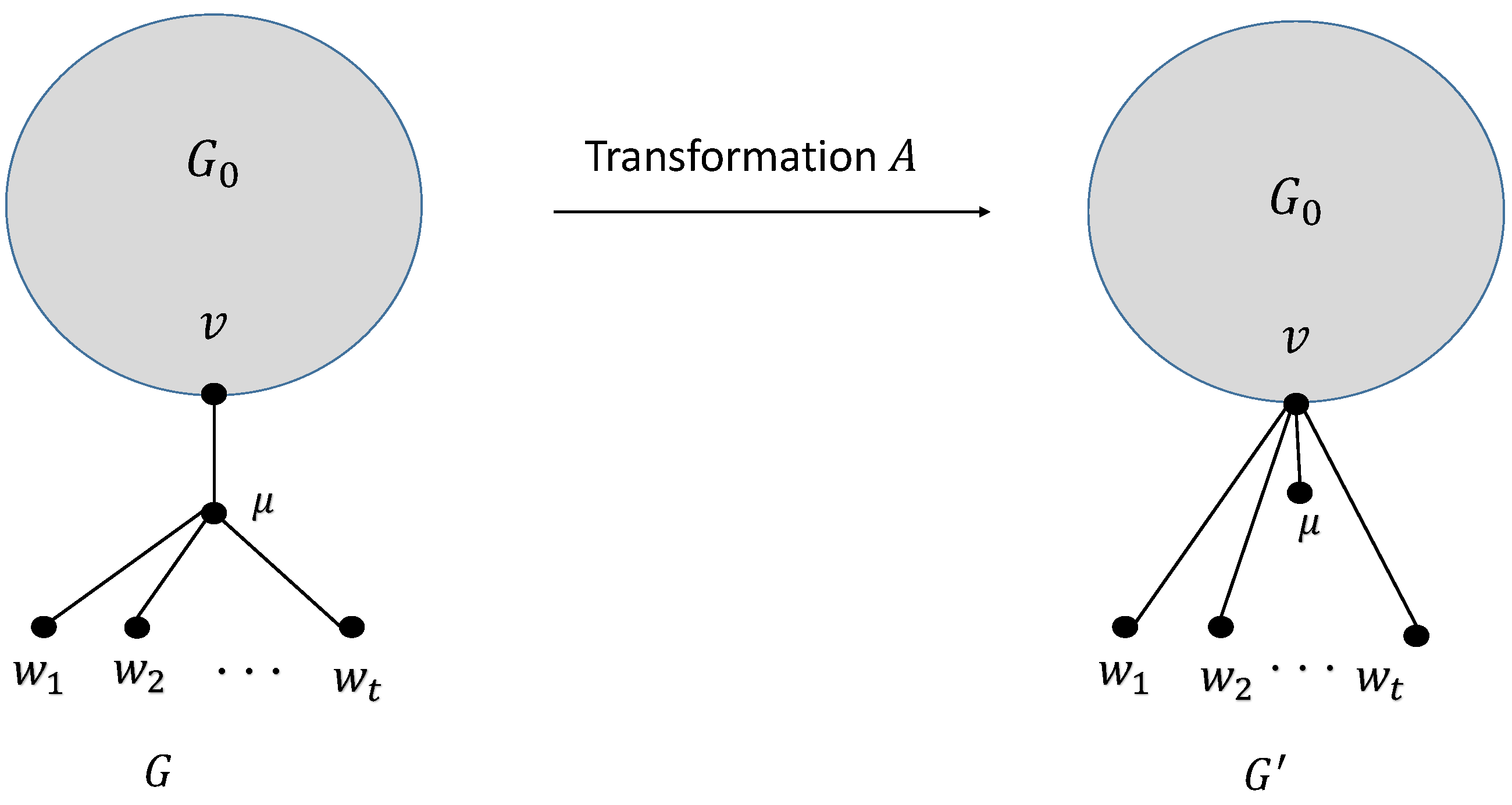
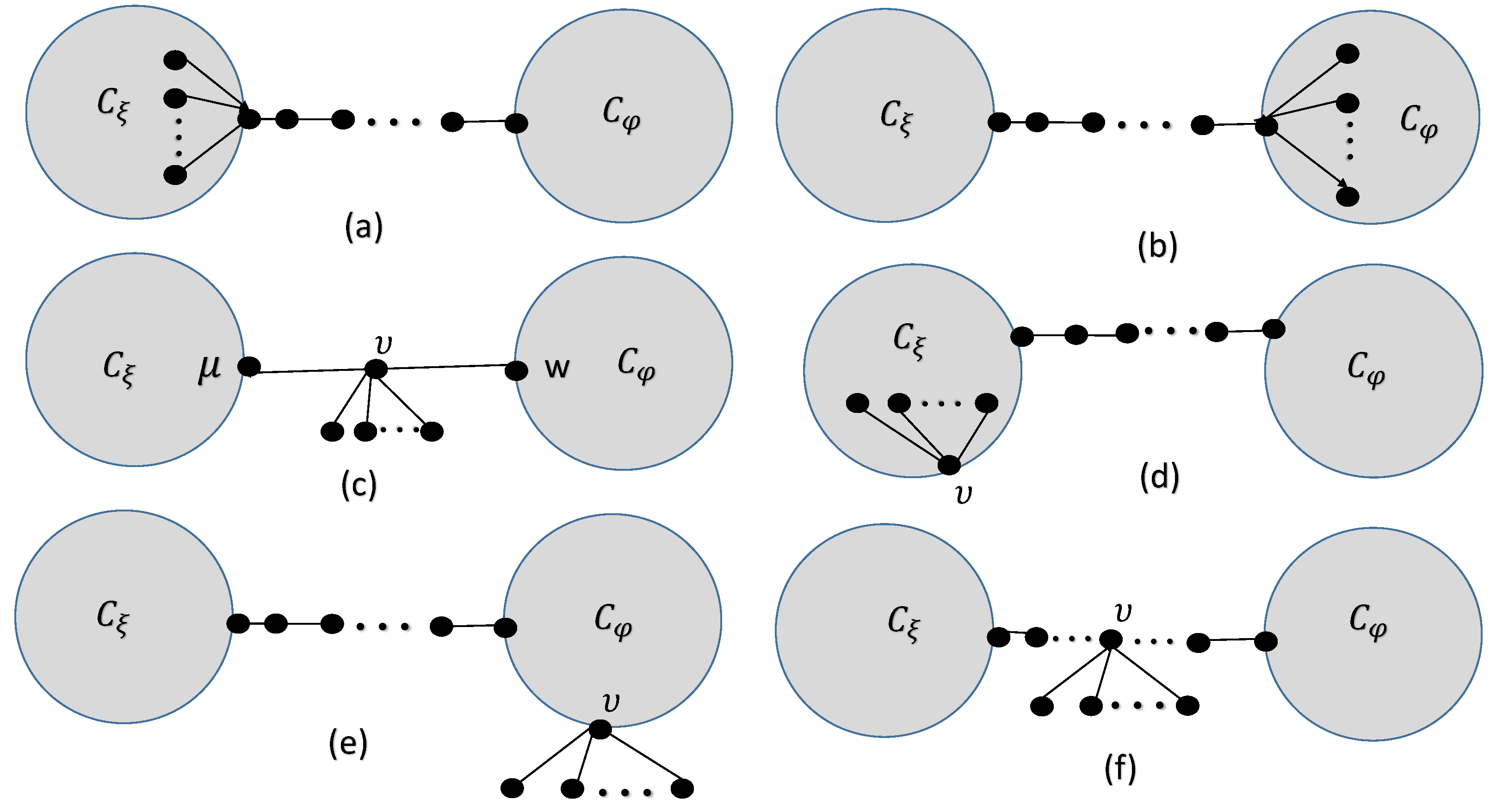
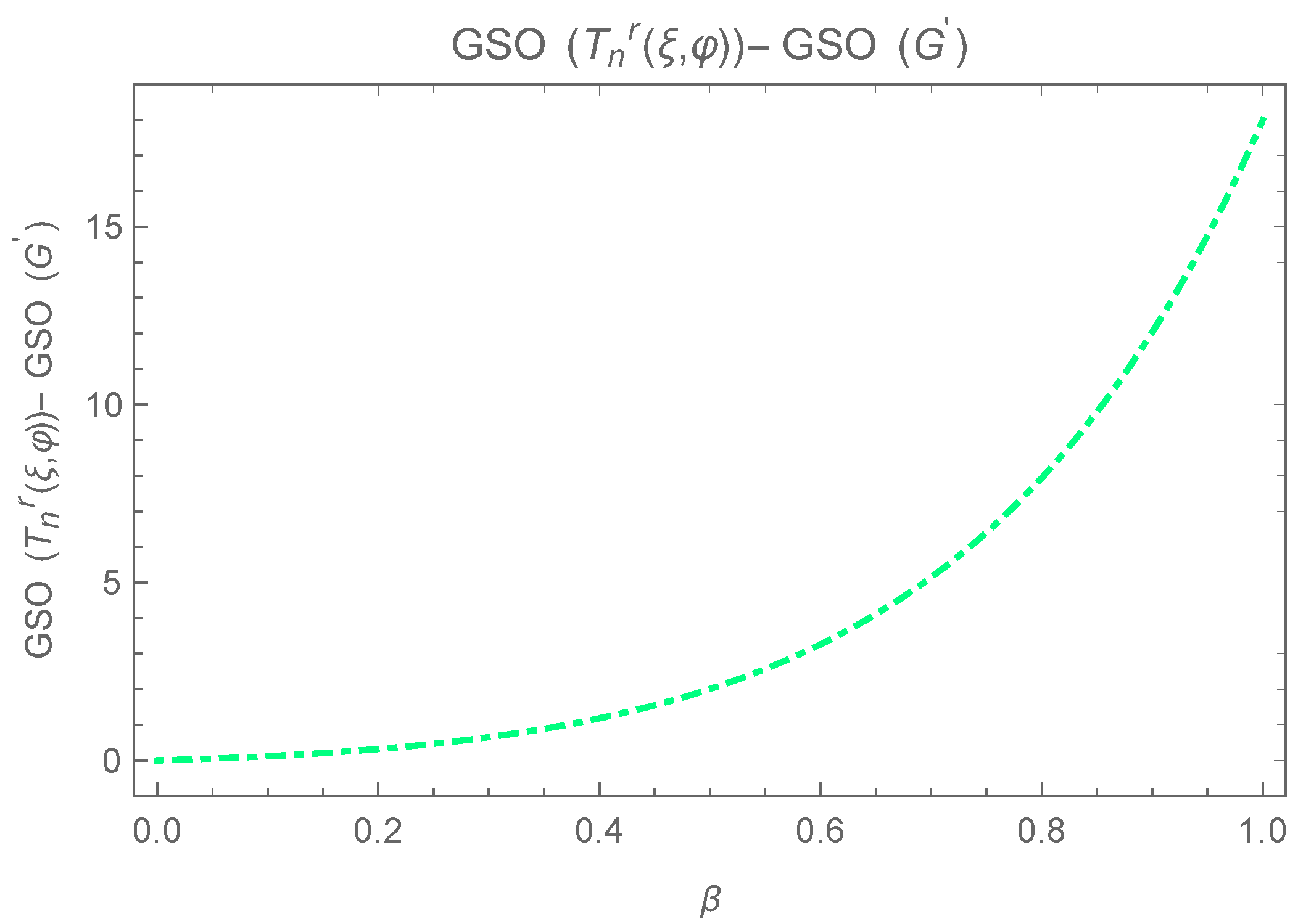
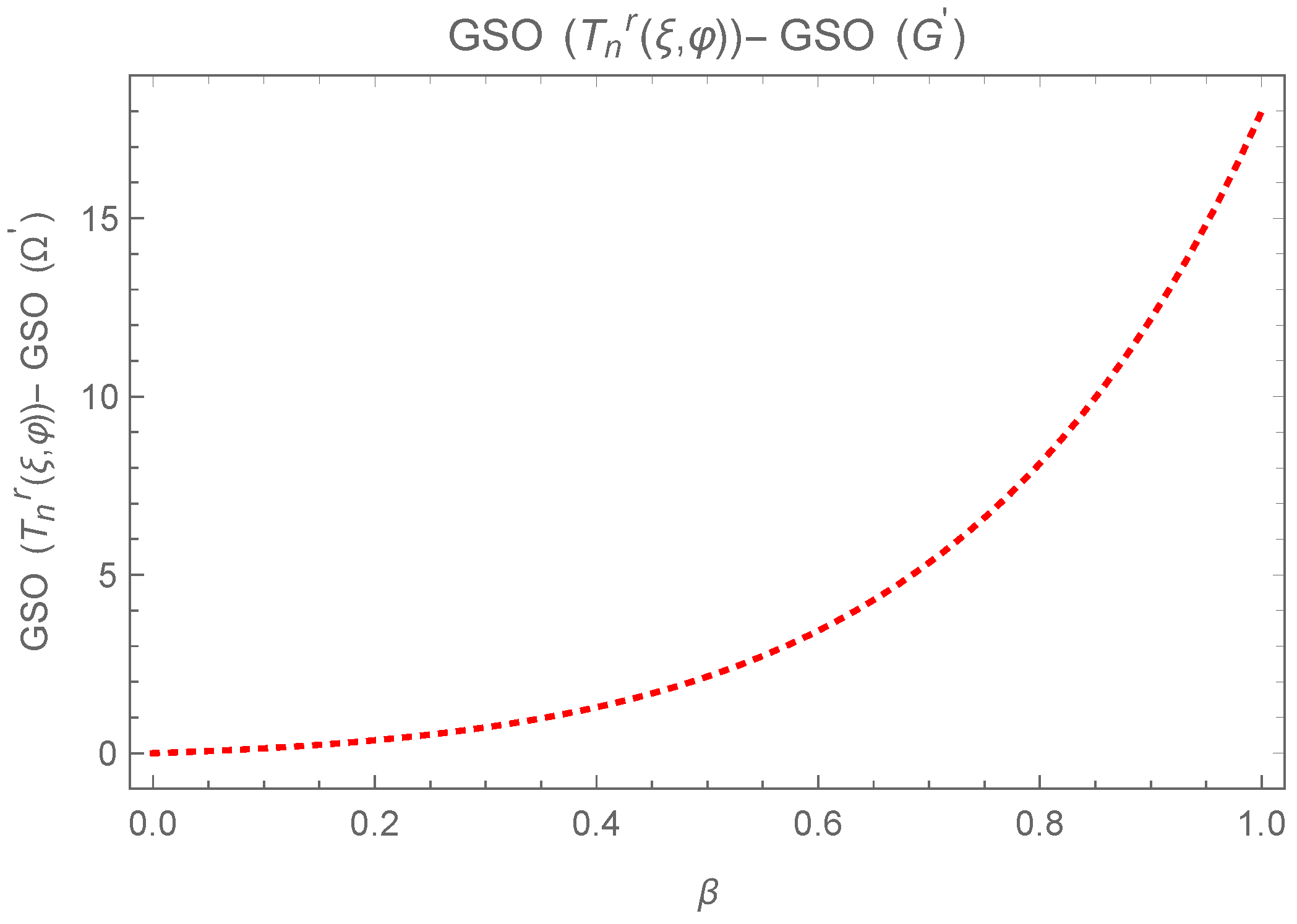
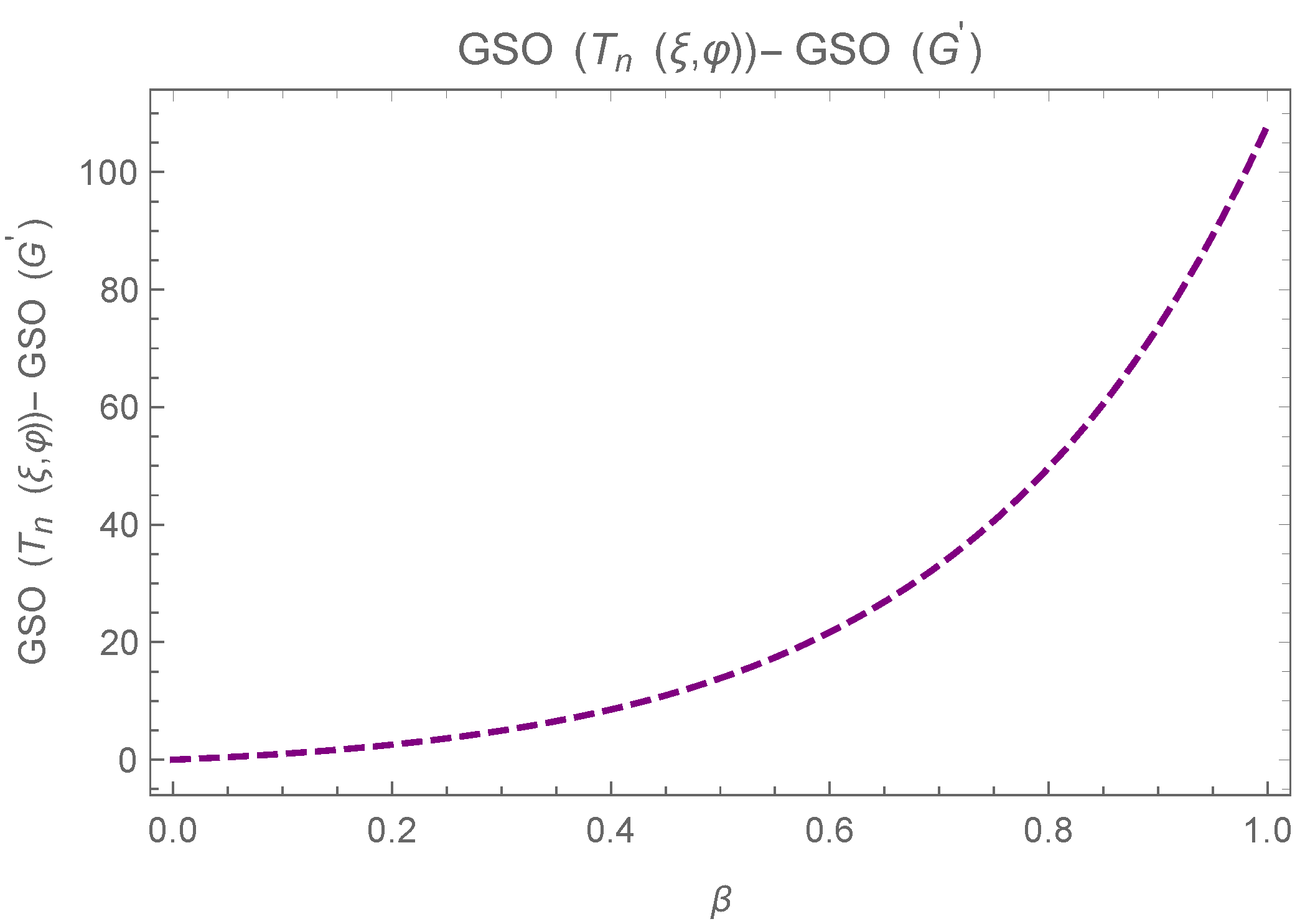
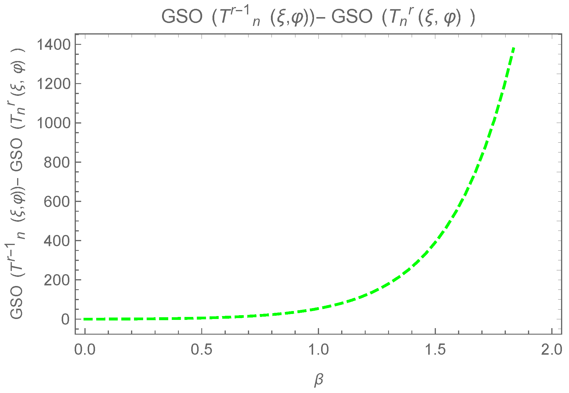
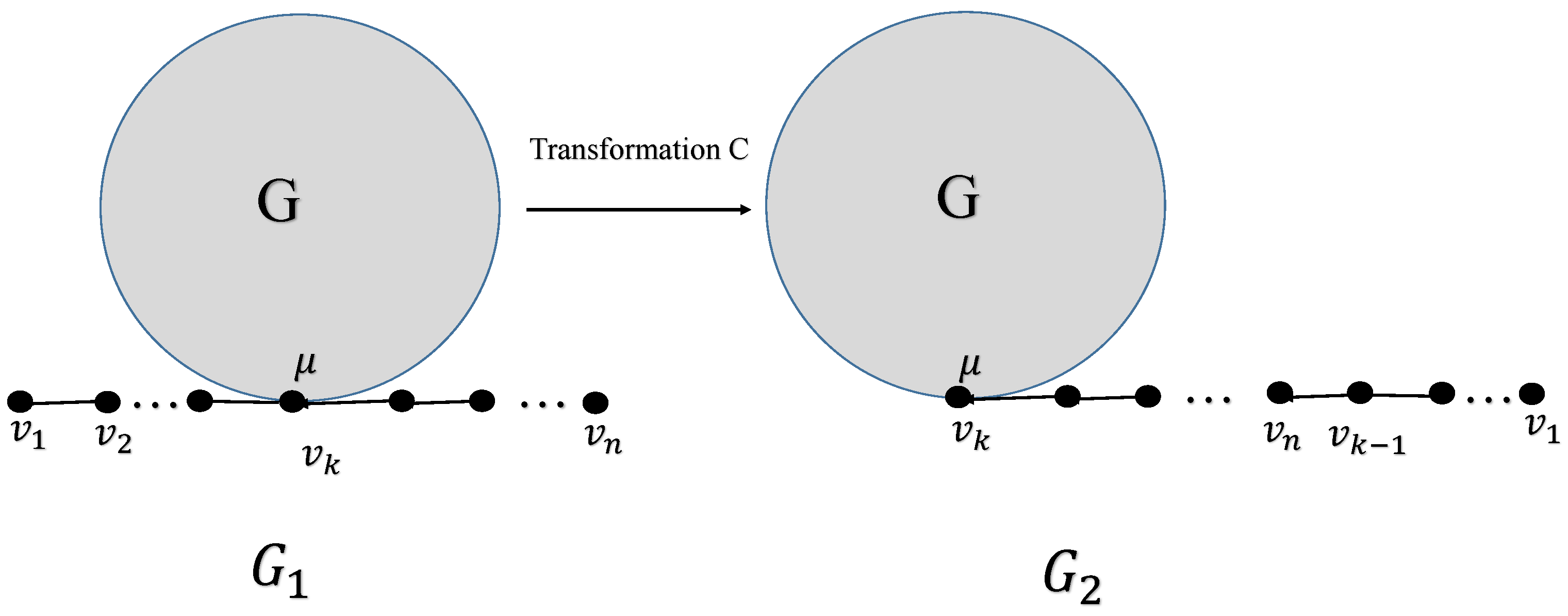
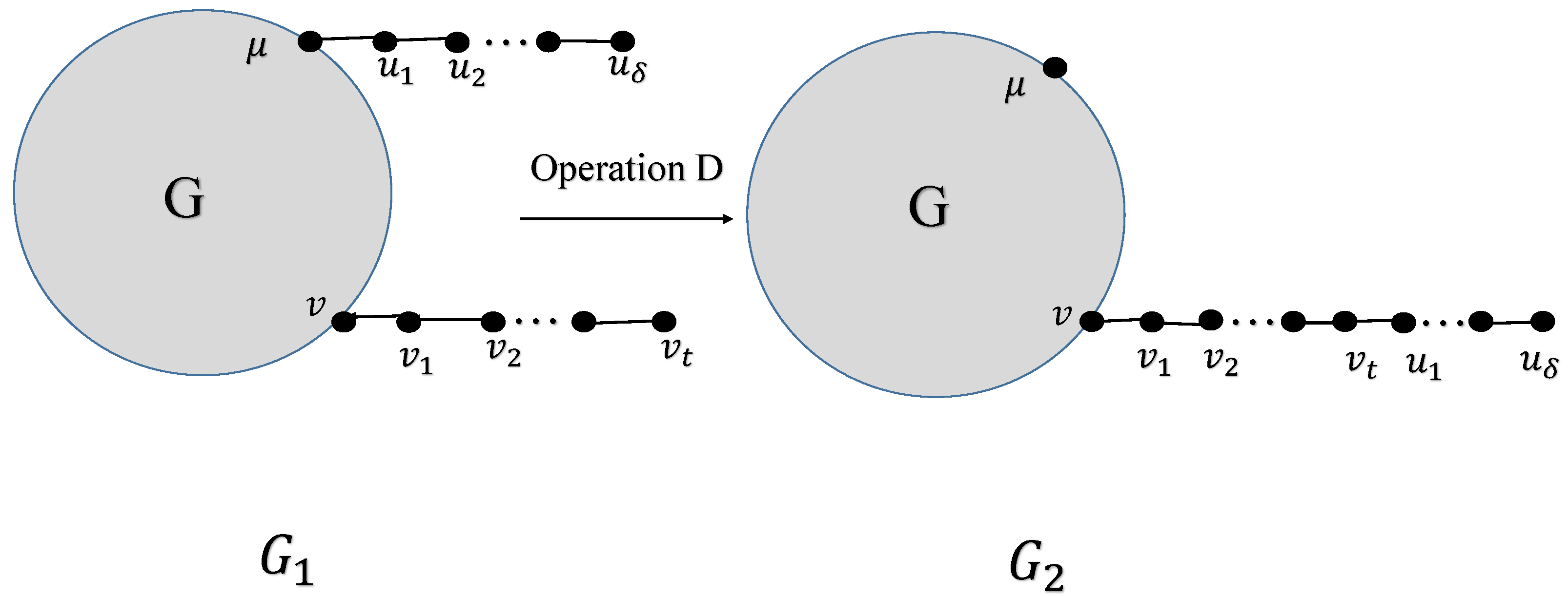
2. Transformation for Greatest Value of Generalized Sombor Index

Transformation A: Let $\mu v\in E\left(G\right)$ with $2\le d\left(v\right)$. Let $N\left(\mu \right)=\{v,w_1,w_2,w_3,\cdots ,w_t\}$. Let $G^{\prime }=G-\{\mu w_1,\mu w_2,\mu w_3,\cdots ,\mu w_t\}+\{v{w}_1,v{w}_2,v{w}_3,\cdots ,v{w}_t\}$ and $w_1,w_2,w_3,\cdots ,w_t$ be vertices of degree one, as in Figure 1.

Lemma 1. 

Let G be a graph, apply Transformation A on G, we obtain $G^{\prime }$ for which the following is true:

$$GSO\left(G^{\prime }\right)>GSO\left(G\right).$$

(1)

Proof. 

Using the definition of $GSO$ for $G^{\prime }$, we obtain

$$\begin{array}{cc}& GSO\left(G^{\prime }\right)=\sum _{\theta \in N_{G_0}\left(v\right)}{({\left(d_{G^{\prime }}\left(v\right)\right)}^2+{\left(d_{G^{\prime }}\left(\theta \right)\right)}^2)}^{\beta }+{({\left(d_{G^{\prime }}\left(v\right)\right)}^2+{\left(d_{G^{\prime }}\left(\mu \right)\right)}^2)}^{\beta }+{({\left(d_{G^{\prime }}\left(v\right)\right)}^2+{\left(d_{G^{\prime }}\left(w_1\right)\right)}^2)}^{\beta }\hfill \\ & +\cdots +{({\left(d_{G^{\prime }}\left(v\right)\right)}^2+{\left(d_{G^{\prime }}\left(w_t\right)\right)}^2)}^{\beta },\hfill \\ & =\sum _{\theta \in N_{G_0}\left(v\right)}{({\left(d_{G^{\prime }}\left(v\right)\right)}^2+{\left(d_{G^{\prime }}\left(\theta \right)\right)}^2)}^{\beta }+(t+1){({\left(d_{G^{\prime }}\left(v\right)\right)}^2+1)}^{\beta }.\hfill \end{array}$$

(2)

Apply $GSO$ on G, we obtain

$$\begin{array}{cc}& GSO\left(G\right)=\sum _{\theta \in N_{G_0}\left(v\right)}{({\left(d_G\left(v\right)\right)}^2+{\left(d_G\left(\theta \right)\right)}^2)}^{\beta }+{({\left(d_G\left(v\right)\right)}^2+{\left(d_G\left(\mu \right)\right)}^2)}^{\beta }+{({\left(d_G\left(\mu \right)\right)}^2+{\left(d_G\left(w_1\right)\right)}^2)}^{\beta }\hfill \\ & +{({\left(d_G\left(\mu \right)\right)}^2+{\left(d_G\left(w_2\right)\right)}^2)}^{\beta }+\cdots +{({\left(d_G\left(\mu \right)\right)}^2+{\left(d_G\left(w_t\right)\right)}^2)}^{\beta },\hfill \\ & =\sum _{\theta \in N_{G_0}\left(v\right)}{({\left(d_G\left(v\right)\right)}^2+{\left(d_G\left(\theta \right)\right)}^2)}^{\beta }+{({\left(d_G\left(v\right)\right)}^2+{\left(d_G\left(\mu \right)\right)}^2)}^{\beta }+t{({\left(d_G\left(\mu \right)\right)}^2+1)}^{\beta }.\hfill \end{array}$$

(3)

We considered the difference (2)–(3), in the following

$$\begin{array}{cc}& GSO\left(G^{\prime }\right)-GSO\left(G\right)=\sum _{\theta \in N_{G_0}\left(v\right)}{({\left(d_{G^{\prime }}\left(v\right)\right)}^2+{\left(d_{G^{\prime }}\left(\theta \right)\right)}^2)}^{\beta }+(t+1){({\left(d_{G^{\prime }}\left(v\right)\right)}^2+1)}^{\beta }\hfill \\ & -\sum _{\theta \in N_{G_0}\left(v\right)}{({\left(d_G\left(v\right)\right)}^2+{\left(d_G\left(\theta \right)\right)}^2)}^{\beta }-{({\left(d_G\left(v\right)\right)}^2+{\left(d_G\left(\mu \right)\right)}^2)}^{\beta }-t{({\left(d_G\left(\mu \right)\right)}^2+1)}^{\beta },\hfill \\ & =\sum _{\theta \in N_{G_0}\left(v\right)}{({\left(d_{G^{\prime }}\left(v\right)\right)}^2+{\left(d_{G^{\prime }}\left(\theta \right)\right)}^2)}^{\beta }+2{({\left(d_{G^{\prime }}\left(v\right)\right)}^2+1^2)}^{\beta }+(t-1){({\left(d_{G^{\prime }}\left(v\right)\right)}^2+1^2)}^{\beta }\hfill \\ & -\sum _{\theta \in N_{G_0}\left(v\right)}{({\left(d_G\left(v\right)\right)}^2+{\left(d_G\left(\theta \right)\right)}^2)}^{\beta }-{({\left(d_G\left(v\right)\right)}^2+{\left(d_G\left(\mu \right)\right)}^2)}^{\beta }-t{({\left(d_G\left(\mu \right)\right)}^2+1^2)}^{\beta },\hfill \\ & >0.\hfill \end{array}$$

(4)

For positive value in Equation (4), it follows that

$$\begin{array}{cc}& \sum _{\theta \in N_{G_0}\left(v\right)}{({\left(d_{G^{\prime }}\left(v\right)\right)}^2+{\left(d_{G^{\prime }}\left(\theta \right)\right)}^2)}^{\beta }>\sum _{\theta \in N_{G_0}\left(v\right)}{({\left(d_G\left(v\right)\right)}^2+{\left(d_G\left(\theta \right)\right)}^2)}^{\beta },\hfill \\ & (t-1){({\left(d_{G^{\prime }}\left(v\right)\right)}^2+1^2)}^{\beta }>t{({\left(d_G\left(\mu \right)\right)}^2+1)}^{\beta }.\hfill \end{array}$$

(5)

As we have the following

$$\begin{array}{cc}& {\left(d_{G^{\prime }}\left(v\right)\right)}^2>{\left(d_G\left(v\right)\right)}^2,{\left(d_{G^{\prime }}\left(v\right)\right)}^2>{\left(d_G\left(\mu \right)\right)}^2,\hfill \\ & \Rightarrow {\left(d_{G^{\prime }}\left(v\right)\right)}^2+1>{\left(d_G\left(v\right)\right)}^2,{\left(d_{G^{\prime }}\left(v\right)\right)}^2+1>{\left(d_G\left(\mu \right)\right)}^2,\hfill \\ & \Rightarrow 2{({\left(d_{G^{\prime }}\left(v\right)\right)}^2+1)}^{\beta }>{({\left(d_G\left(v\right)\right)}^2+{\left(d_G\left(\mu \right)\right)}^2)}^{\beta }.\hfill \end{array}$$

(6)

From Equations (5) and (6), we obtain

$$GSO\left(G^{\prime }\right)>GSO\left(G\right).$$

□

Remark 1. 

Using Transformation A repeatedly, we transform any tree to a star and bicyclic or unicyclic graphs to bicyclic or unicyclic graphs where all the non-cyclic edges are pendent, respectively.

Transformation B: Consider $\mu ,v\in V\left(G\right)$. Let adjacent leaves to $\mu$ be $u_{\delta },u_{\delta -1},\cdots ,u_2,u_1$. Let adjacent leaves to v be $v_t,v_{t-1},\cdots ,v_2,v_1$, $G^{\prime }$ and $G^{″}$ are obtained such that $G^{\prime }=G+\{v{u}_1,v{u}_2,\cdots ,v{u}_{\delta }\}-\{\mu u_1,\mu u_2,\cdots ,\mu u_{\delta }\}$ and $G^{″}=G-\{v{v}_1,v{v}_2,\cdots ,v{v}_t\}+\{\mu v_1,\mu v_2,$$\cdots ,\mu v_t\}$, as shown in the Figure 2.

Lemma 2. 

Consider graph G. Using Transformation B on G, we obtain $G^{\prime }$ and $G^{″}$, then either $GSO\left(G^{\prime }\right)>GSO\left(G\right)$ or $GSO\left(G^{″}\right)>GSO\left(G\right)$.

Proof. 

Consider $G_0=\{v_t,v_{t-1},\cdots ,v_2,v_1,u_{\delta },u_{\delta -1},\cdots ,u_2,u_1\}$. The following cases are considered for G, $G^{\prime }$ and $G^{″}$.

Let $d_{G_0}\left(\mu \right)=\xi$ and $d_{G_0}\left(v\right)=\phi$.

• Case 1. Consider G, if v and $\mu$ are not connected directly by an edge, then for $GSO$ we have

  $$\begin{array}{cc}& GSO\left(G\right)=\sum _{\theta y\in E(G-\{\mu ,v\left\}\right)}{({\left(d_{G_0}\left(\theta \right)\right)}^2+{\left(d_{G_0}\left(y\right)\right)}^2)}^{\beta }+\sum _{\theta \in N_{G_0}\left(\mu \right)}{({\left(d_G\left(\mu \right)\right)}^2+{\left(d_{G_0}\left(\theta \right)\right)}^2)}^{\beta }\hfill \\ & +\sum _{\theta \in N_{G_0}\left(v\right)}{({\left(d_G\left(v\right)\right)}^2+{\left(d_{G_0}\left(\theta \right)\right)}^2)}^{\beta }+{({\left(d_G\left(\mu \right)\right)}^2+1)}^{\beta }+{({\left(d_G\left(\mu \right)\right)}^2+1)}^{\beta }\hfill \\ & +\cdots +{({\left(d_G\left(\mu \right)\right)}^2+1)}^{\beta }+{({\left(d_G\left(v\right)\right)}^2+1)}^{\beta }+{({\left(d_G\left(v\right)\right)}^2+1)}^{\beta }+\cdots +{({\left(d_G\left(v\right)\right)}^2+1)}^{\beta },\hfill \\ & =\sum _{\theta y\in E(G-\{\mu ,v\left\}\right)}{({\left(d_{G_0}\left(\theta \right)\right)}^2+{\left(d_{G_0}\left(y\right)\right)}^2)}^{\beta }+\sum _{\theta \in N_{G_0}\left(\mu \right)}{({(\xi +\delta )}^2+{\left(d_{G_0}\left(\theta \right)\right)}^2)}^{\beta }\hfill \\ & +\sum _{\theta \in N_{G_0}\left(v\right)}{({(\phi +t)}^2+{\left(d_{G_0}\left(\theta \right)\right)}^2)}^{\beta }+\delta {({(\xi +\delta )}^2+1)}^{\beta }+t{({(\phi +t)}^2+1)}^{\beta }.\hfill \end{array}$$

  (7)

  Consider $G^{\prime }$, then $GSO$ is given by

  $$\begin{array}{cc}& GSO\left(G^{\prime }\right)=\sum _{\theta y\in E(G-\{\mu ,v\left\}\right)}{({\left(d_{G_0}\left(\theta \right)\right)}^2+{\left(d_{G_0}\left(y\right)\right)}^2)}^{\beta }+\sum _{\theta \in N_{G_0}\left(\mu \right)}{(d_{G_0}{\left(\mu \right)}^2+{\left(d_{G_0}\left(\theta \right)\right)}^2)}^{\beta }\hfill \\ & +\sum _{\theta \in N_{G_0}\left(v\right)}{({\left(d_{G^{\prime }}\left(v\right)\right)}^2+{\left(d_{G_0}\left(\theta \right)\right)}^2)}^{\beta }+{({\left(d_{G^{\prime }}\left(v\right)\right)}^2+1)}^{\beta }+\cdots +{({\left(d_{G^{\prime }}\left(v\right)\right)}^2+1)}^{\beta },\hfill \\ & =\sum _{\theta y\in E(G-\{\mu ,v\left\}\right)}{({\left(d_{G_0}\left(\theta \right)\right)}^2+{\left(d_{G_0}\left(y\right)\right)}^2)}^{\beta }+\sum _{\theta \in N_{G_0}\left(\mu \right)}{({\xi }^2+{\left(d_{G_0}\left(\theta \right)\right)}^2)}^{\beta }\hfill \\ & +\sum _{\theta \in N_{G_0}\left(v\right)}{({(\phi +\delta +t)}^2+{\left(d_{G_0}\left(\theta \right)\right)}^2)}^{\beta }+(\delta +t){({(\phi +\delta +t)}^2+1)}^{\beta }.\hfill \end{array}$$

  Taking $G^{″}$, then $GSO$ is in the following

  $$\begin{array}{cc}& GSO\left(G^{″}\right)=\sum _{\theta y\in E(G-\{\mu ,v\left\}\right)}{({\left(d_{G_0}\left(\theta \right)\right)}^2+{\left(d_{G_0}\left(y\right)\right)}^2)}^{\beta }+\sum _{\theta \in N_{G_0}\left(\mu \right)}{(d_{G^{″}}{\left(\mu \right)}^2+{\left(d_{G_0}\left(\theta \right)\right)}^2)}^{\beta }\hfill \\ & +\sum _{\theta \in N_{G_0}\left(v\right)}{(d_{G_0}{\left(v\right)}^2+{\left(d_{G_0}\left(\theta \right)\right)}^2)}^{\beta }+{(d_{G^{″}}{\left(\mu \right)}^2+1)}^{\beta }+\cdots +{(d_{G^{″}}{\left(\mu \right)}^2+1)}^{\beta },\hfill \\ & =\sum _{\theta y\in E(G-\{\mu ,v\left\}\right)}{({\left(d_{G_0}\left(\theta \right)\right)}^2+{\left(d_{G_0}\left(y\right)\right)}^2)}^{\beta }+\sum _{\theta \in N_{G_0}\left(\mu \right)}{({(\xi +\delta +t)}^2+{\left(d_{G_0}\left(\theta \right)\right)}^2)}^{\beta }\hfill \\ & +\sum _{\theta \in N_{G_0}\left(v\right)}{({\phi }^2+{\left(d_{G_0}\left(\theta \right)\right)}^2)}^{\beta }+(\delta +t){({(\xi +\delta +t)}^2+1)}^{\beta }.\hfill \end{array}$$

  Suppose ${\Omega }_1=GSO\left(G^{\prime }\right)-GSO\left(G\right)$ and ${\Omega }_2=GSO\left(G^{″}\right)-GSO\left(G\right)$, we consider the following

  $$\begin{array}{cc}& {\Omega }_1=\sum _{\theta y\in E(G-\{\mu ,v\left\}\right)}{({\left(d_{G_0}\left(\theta \right)\right)}^2+{\left(d_{G_0}\left(y\right)\right)}^2)}^{\beta }+\sum _{\theta \in N_{G_0}\left(\mu \right)}{({\xi }^2+{\left(d_{G_0}\left(\theta \right)\right)}^2)}^{\beta }\hfill \\ & +\sum _{\theta \in N_{G_0}\left(v\right)}{({(\phi +\delta +t)}^2+{\left(d_{G_0}\left(\theta \right)\right)}^2)}^{\beta }+(\delta +t){({(\phi +\delta +t)}^2+1)}^{\beta }\hfill \\ & -\sum _{\theta y\in E(G-\{\mu ,v\left\}\right)}{({\left(d_{G_0}\left(\theta \right)\right)}^2+{\left(d_{G_0}\left(y\right)\right)}^2)}^{\beta }-\sum _{\theta \in N_{G_0}\left(\mu \right)}{({(\xi +\delta )}^2+{\left(d_{G_0}\left(\theta \right)\right)}^2)}^{\beta }\hfill \\ & -\sum _{\theta \in N_{G_0}\left(v\right)}{({(\phi +t)}^2+{\left(d_{G_0}\left(\theta \right)\right)}^2)}^{\beta }-\delta {({(\xi +\delta )}^2+1)}^{\beta }-t{({(\phi +t)}^2+1)}^{\beta },\hfill \\ & =\sum _{\theta \in N_{G_0}\left(\mu \right)}{({\xi }^2+{\left(d_{G_0}\left(\theta \right)\right)}^2)}^{\beta }+{({(\phi +\delta +t)}^2+\sum _{\theta \in N_{G_0}\left(v\right)}{\left(d_{G_0}\left(\theta \right)\right)}^2)}^{\beta }\hfill \\ & +(\delta +t){({(\phi +\delta +t)}^2+1)}^{\beta }-\sum _{\theta \in N_{G_0}\left(\mu \right)}{({(\xi +\delta )}^2+{\left(d_{G_0}\left(\theta \right)\right)}^2)}^{\beta }\hfill \\ & -\sum _{\theta \in N_{G_0}\left(v\right)}{({(\phi +t)}^2+{\left(d_{G_0}\left(\theta \right)\right)}^2)}^{\beta }-\delta {({(\xi +\delta )}^2+1)}^{\beta }-t{({(\phi +t)}^2+1)}^{\beta }.\hfill \end{array}$$

  (8)

  Now ${\Omega }_1>0$, if the following holds

  $$\begin{array}{cc}& \sum _{\theta \in N_{G_0}\left(\mu \right)}{({\xi }^2+{\left(d_{G_0}\left(\theta \right)\right)}^2)}^{\beta }+\sum _{\theta \in N_{G_0}\left(v\right)}{({(\phi +\delta +t)}^2+{\left(d_{G_0}\left(\theta \right)\right)}^2)}^{\beta }\hfill \\ & +(\delta +t){({(\phi +\delta +t)}^2+1)}^{\beta }\hfill \\ & >[\sum _{\theta \in N_{G_0}\left(\mu \right)}{({(\xi +\delta )}^2+{\left(d_{G_0}\left(\theta \right)\right)}^2)}^{\beta }+\sum _{\theta \in N_{G_0}\left(v\right)}{({(\phi +t)}^2+{\left(d_{G_0}\left(\theta \right)\right)}^2)}^{\beta }\hfill \\ & \delta {({(\xi +\delta )}^2+1)}^{\beta }+t{({(\phi +t)}^2+1)}^{\beta }],\hfill \\ & \Rightarrow \sum _{\theta \in N_{G_0}\left(\mu \right)}{({(\xi +\delta +t)}^2+{\left(d_{G_0}\left(\theta \right)\right)}^2)}^{\beta }+\sum _{\theta \in N_{G_0}\left(v\right)}{({(\phi +\delta +t)}^2+{\left(d_{G_0}\left(\theta \right)\right)}^2)}^{\beta }\hfill \\ & +(\delta +t){({(\phi +\delta +t)}^2+1)}^{\beta }\hfill \\ & >[\sum _{\theta \in N_{G_0}\left(\mu \right)}{({(\xi +\delta )}^2+{\left(d_{G_0}\left(\theta \right)\right)}^2)}^{\beta }+\sum _{\theta \in N_{G_0}\left(v\right)}{({(\phi +t)}^2+{\left(d_{G_0}\left(\theta \right)\right)}^2)}^{\beta }\hfill \\ & \delta {({(\xi +\delta )}^2+1)}^{\beta }+t{({(\phi +t)}^2+1)}^{\beta }].\hfill \end{array}$$

  (9)

  If ${\Omega }_1>0$ then ${\Omega }_2<0$, we have the following for this

  $$\begin{array}{cc}& {\Omega }_2=\sum _{\theta y\in E(G-\{\mu ,v\left\}\right)}{({\left(d_{G_0}\left(\theta \right)\right)}^2+{\left(d_{G_0}\left(y\right)\right)}^2)}^{\beta }+\sum _{\theta \in N_{G_0}\left(\mu \right)}{({(\xi +\delta +t)}^2+{\left(d_{G_0}\left(\theta \right)\right)}^2)}^{\beta }\hfill \\ & +\sum _{\theta \in N_{G_0}\left(v\right)}{({\phi }^2+{\left(d_{G_0}\left(\theta \right)\right)}^2)}^{\beta }+(\delta +t){({(\xi +\delta +t)}^2+1)}^{\beta }\hfill \\ & -\sum _{\theta y\in E(G-\{\mu ,v\left\}\right)}{({\left(d_{G_0}\left(\theta \right)\right)}^2+{\left(d_{G_0}\left(y\right)\right)}^2)}^{\beta }+\sum _{\theta \in N_{G_0}\left(\mu \right)}{({(\xi +\delta )}^2+{\left(d_{G_0}\left(\theta \right)\right)}^2)}^{\beta }\hfill \\ & +\sum _{\theta \in N_{G_0}\left(v\right)}{({(\phi +t)}^2+{\left(d_{G_0}\left(\theta \right)\right)}^2)}^{\beta }\delta {({(\xi +\delta )}^2+1)}^{\beta }+t{({(\phi +t)}^2+1)}^{\beta },\hfill \\ & =\sum _{\theta \in N_{G_0}\left(v\right)}{({\phi }^2+{\left(d_{G_0}\left(\theta \right)\right)}^2)}^{\beta }-\sum _{\theta \in N_{G_0}\left(v\right)}{({(\phi +\delta +t)}^2+{\left(d_{G_0}\left(\theta \right)\right)}^2)}^{\beta }<0.\hfill \end{array}$$

  (10)
• Case 2. Consider graph G, if v and $\mu$ are connected directly by an edge, then we obtain

  $$\begin{array}{cc}& GSO\left(G\right)=\sum _{\theta y\in E(G-\{\mu ,v\left\}\right)}{({\left(d_{G_0}\left(\theta \right)\right)}^2+{\left(d_{G_0}\left(y\right)\right)}^2)}^{\beta }+\sum _{\theta \in N_{G_0}\left(\mu \right)}{({(\xi +\delta )}^2+{\left(d_{G_0}\left(\theta \right)\right)}^2)}^{\beta }\hfill \\ & +\sum _{\theta \in N_{G_0}\left(v\right)}{({(\phi +t)}^2+{\left(d_{G_0}\left(\theta \right)\right)}^2)}^{\beta }+{({(\xi +\delta )}^2+1)}^{\beta }+\cdots +{({(\xi +\delta )}^2+1)}^{\beta }\hfill \\ & +{({(\phi +t)}^2+1)}^{\beta }+\cdots +{({(\phi +t)}^2+1)}^{\beta }-{({(\xi +\delta )}^2+{(\phi +t)}^2)}^{\beta },\hfill \\ & =\sum _{\theta y\in E(G-\{\mu ,v\left\}\right)}{({\left(d_{G_0}\left(\theta \right)\right)}^2+{\left(d_{G_0}\left(y\right)\right)}^2)}^{\beta }+\sum _{\theta \in N_{G_0}\left(\mu \right)}{({(\xi +\delta )}^2+{\left(d_{G_0}\left(\theta \right)\right)}^2)}^{\beta }\hfill \\ & +\sum _{\theta \in N_{G_0}\left(v\right)}{({(\phi +t)}^2+{\left(d_{G_0}\left(\theta \right)\right)}^2)}^{\beta }\delta {({(\xi +\delta )}^2+1)}^{\beta }+t{({(\phi +t)}^2+1)}^{\beta }\hfill \\ & -{({(\xi +\delta )}^2+{(\phi +t)}^2)}^{\beta }.\hfill \end{array}$$

  (11)

  $GSO$ for $G^{\prime }$ is given in Equation (12)

  $$\begin{array}{cc}& GSO\left(G^{\prime }\right)=\sum _{\theta y\in E(G-\{\mu ,v\left\}\right)}{({\left(d_{G_0}\left(\theta \right)\right)}^2+{\left(d_{G_0}\left(y\right)\right)}^2)}^{\beta }+\sum _{\theta \in N_{G_0}\left(\mu \right)}{({\xi }^2+{\left(d_{G_0}\left(\theta \right)\right)}^2)}^{\beta }\hfill \\ & +\sum _{\theta \in N_{G_0}\left(v\right)}{({(\phi +\delta +t)}^2+{\left(d_{G_0}\left(\theta \right)\right)}^2)}^{\beta }+{({(\phi +\delta +t)}^2+1)}^{\beta }+\cdots \hfill \\ & +{({(\phi +\delta +t)}^2+1)}^{\beta }-{({\xi }^2+{(\phi +\delta +t)}^2)}^{\beta },\hfill \\ & =\sum _{\theta y\in E(G-\{\mu ,v\left\}\right)}{({\left(d_{G_0}\left(\theta \right)\right)}^2+{\left(d_{G_0}\left(y\right)\right)}^2)}^{\beta }+\sum _{\theta \in N_{G_0}\left(\mu \right)}{({\left(\xi \right)}^p+{\left(d_{G_0}\left(\theta \right)\right)}^2)}^{\beta }\hfill \\ & +\sum _{\theta \in N_{G_0}\left(v\right)}{({(\phi +\delta +t)}^2+{\left(d_{G_0}\left(\theta \right)\right)}^2)}^{\beta }+(\delta +t){({(\phi +\delta +t)}^2+1)}^{\beta }\hfill \\ & -{({\xi }^2+{(\phi +\delta +t)}^2)}^{\beta }.\hfill \end{array}$$

  (12)

  $GSO$ for $G^{″}$ is considered in Equation (13)

  $$\begin{array}{cc}& GSO\left(G^{″}\right)=\sum _{\theta y\in E(G-\{\mu ,v\left\}\right)}{({\left(d_{G_0}\left(\theta \right)\right)}^2+{\left(d_{G_0}\left(y\right)\right)}^2)}^{\beta }+\sum _{\theta \in N_{G_0}\left(\mu \right)}{({(\xi +\delta +t)}^2+{\left(d_{G_0}\left(\theta \right)\right)}^2)}^{\beta }\hfill \\ & +\sum _{\theta \in N_{G_0}\left(v\right)}{({\phi }^2+{\left(d_{G_0}\left(\theta \right)\right)}^2)}^{\beta }+{({(\xi +\delta +t)}^2+1)}^{\beta }+\cdots \hfill \\ & +{({(\delta +\xi +t)}^2+1)}^{\beta }-{({(\xi +\delta +t)}^2+q^2)}^{\beta },\hfill \\ & =\sum _{\theta y\in E(G-\{\mu ,v\left\}\right)}{({\left(d_{G_0}\left(\theta \right)\right)}^2+{\left(d_{G_0}\left(y\right)\right)}^2)}^{\beta }+\sum _{\theta \in N_{G_0}\left(\mu \right)}{({(\xi +\delta +t)}^2+{\left(d_{G_0}\left(\theta \right)\right)}^2)}^{\beta }\hfill \\ & +\sum _{\theta \in N_{G_0}\left(v\right)}{({\phi }^2+{\left(d_{G_0}\left(\theta \right)\right)}^2)}^{\beta }+(\delta +t){({(\delta +\xi +t)}^2+1)}^{\beta }-{({(\delta +\xi +t)}^2+q^2)}^{\beta }.\hfill \end{array}$$

  (13)

  Let ${\Omega }_1=GSO\left(G^{\prime }\right)-GSO\left(G\right)$ and ${\Omega }_2=GSO\left(G^{″}\right)-GSO\left(G\right)$, we consider the following

  $$\begin{array}{cc}& {\Omega }_1=\sum _{\theta y\in E(G-\{\mu ,v\left\}\right)}{({\left(d_{G_0}\left(\theta \right)\right)}^2+{\left(d_{G_0}\left(y\right)\right)}^2)}^{\beta }+\sum _{\theta \in N_{G_0}\left(\mu \right)}{({\left(\xi \right)}^2+{\left(d_{G_0}\left(\theta \right)\right)}^2)}^{\beta }\hfill \\ & +\sum _{\theta \in N_{G_0}\left(v\right)}{({(\phi +\delta +t)}^2+{\left(d_{G_0}\left(\theta \right)\right)}^2)}^{\beta }+(\delta +t){({(\phi +\delta +t)}^2+1)}^{\beta }\hfill \\ & -{({\xi }^2+{(\phi +\delta +t)}^2)}^{\beta }\hfill \\ & -\sum _{\theta y\in E(G-\{\mu ,v\left\}\right)}{({\left(d_{G_0}\left(\theta \right)\right)}^2+{\left(d_{G_0}\left(y\right)\right)}^2)}^{\beta }-\sum _{\theta \in N_{G_0}\left(\mu \right)}{({(\xi +\delta )}^2+{\left(d_{G_0}\left(\theta \right)\right)}^2)}^{\beta }\hfill \\ & -\sum _{\theta \in N_{G_0}\left(v\right)}{({(\phi +t)}^2+{\left(d_{G_0}\left(\theta \right)\right)}^2)}^{\beta }-\delta {({(\xi +\delta )}^2+1)}^{\beta }-t{({(\phi +t)}^2+1)}^{\beta }\hfill \\ & +{({(\xi +\delta )}^2+{(\phi +t)}^2)}^{\beta }.\hfill \end{array}$$

  $$\begin{array}{cc}& {\Omega }_1={({\xi }^2+\sum _{\theta \in N_{G_0}\left(\mu \right)}{\left(d_{G_0}\left(\theta \right)\right)}^2)}^{\beta }+\sum _{\theta \in N_{G_0}\left(v\right)}{({(\phi +\delta +t)}^2+{\left(d_{G_0}\left(\theta \right)\right)}^2)}^{\beta }\hfill \\ & +(\delta +t){({(\phi +\delta +t)}^2+1)}^{\beta }-{({\xi }^2+{(\phi +\delta +t)}^2)}^{\beta }\hfill \\ & -\sum _{\theta \in N_{G_0}\left(\mu \right)}{({(\xi +\delta )}^2+{\left(d_{G_0}\left(\theta \right)\right)}^2)}^{\beta }-\sum _{\theta \in N_{G_0}\left(v\right)}{({(\phi +t)}^2+{\left(d_{G_0}\left(\theta \right)\right)}^2)}^{\beta }\hfill \\ & -\delta {({(\xi +\delta )}^2+1)}^{\beta }-t{({(\phi +t)}^2+1)}^{\beta }+{({(\xi +\delta )}^2+{(\phi +t)}^2)}^{\beta },\hfill \\ & =\sum _{\theta \in N_{G_0}\left(\mu \right)}{({\xi }^2+{\left(d_{G_0}\left(\theta \right)\right)}^2)}^{\beta }+\sum _{\theta \in N_{G_0}\left(v\right)}{({(\phi +\delta +t)}^2+{\left(d_{G_0}\left(\theta \right)\right)}^2)}^{\beta }\hfill \\ & +(\delta +t){({(\phi +\delta +t)}^2+1)}^{\beta }+{({(\xi +\delta )}^2+{(\phi +t)}^2)}^{\beta }\hfill \\ & -{({\xi }^2+{(\phi +\delta +t)}^2)}^{\beta }-\sum _{\theta \in N_{G_0}\left(\mu \right)}{({(\xi +\delta )}^2+{\left(d_{G_0}\left(\theta \right)\right)}^2)}^{\beta }\hfill \\ & -\sum _{\theta \in N_{G_0}\left(v\right)}{({(\phi +t)}^2+{\left(d_{G_0}\left(\theta \right)\right)}^2)}^{\beta }-\delta {({(\xi +\delta )}^2+1)}^{\beta }-t{({(\phi +t)}^2+1)}^{\beta }.\hfill \end{array}$$

  (14)

  If ${\Omega }_1>0$, then it follows that

  $$\begin{array}{cc}& \sum _{\theta \in N_{G_0}\left(\mu \right)}{({\xi }^2+{\left(d_{G_0}\left(\theta \right)\right)}^2)}^{\beta }+\sum _{\theta \in N_{G_0}\left(v\right)}{({(\phi +\delta +t)}^2+{\left(d_{G_0}\left(\theta \right)\right)}^2)}^{\beta }\hfill \\ & +(\delta +t){({(\phi +\delta +t)}^2+1)}^{\beta }+{({(\xi +\delta )}^2+{(\phi +t)}^2)}^{\beta }\hfill \\ & >-{({\xi }^2+{(\phi +\delta +t)}^2)}^{\beta }-\sum _{\theta \in N_{G_0}\left(\mu \right)}{({(\xi +\delta )}^2+{\left(d_{G_0}\left(\theta \right)\right)}^2)}^{\beta }\hfill \\ & -\sum _{\theta \in N_{G_0}\left(v\right)}{({(\phi +t)}^2+{\left(d_{G_0}\left(\theta \right)\right)}^2)}^{\beta }-\delta {({(\xi +\delta )}^2+1)}^{\beta }-t{({(\phi +t)}^2+1)}^{\beta }.\hfill \end{array}$$

  $$\begin{array}{cc}& \Rightarrow \sum _{\theta \in N_{G_0}\left(\mu \right)}{({(\xi +\delta +t)}^2+{\left(d_{G_0}\left(\theta \right)\right)}^2)}^{\beta }+\sum _{\theta \in N_{G_0}\left(v\right)}{({(\phi +\delta +t)}^2+{\left(d_{G_0}\left(\theta \right)\right)}^2)}^{\beta }\hfill \\ & +(\delta +t){({(\phi +\delta +t)}^2+{(\delta +\xi +t)}^2)}^{\beta }+{({(\delta +\xi )}^2+(\phi +t\delta ))}^{\beta }\hfill \\ & >-{({\xi }^2+{(\phi +t+\delta )}^2)}^{\beta }-\sum _{\theta \in N_{G_0}\left(\mu \right)}{({(\delta +\xi )}^2+{\left(d_{G_0}\left(\theta \right)\right)}^2)}^{\beta }\hfill \\ & -\sum _{\theta \in N_{G_0}\left(v\right)}{({(\phi +t)}^2+{\left(d_{G_0}\left(\theta \right)\right)}^2)}^{\beta }-\delta {({(\xi +\delta )}^2+1)}^{\beta }-t{({(\phi +t)}^2+1)}^{\beta }.\hfill \end{array}$$

  (15)

  When (15) satisfies, then we get the following

  $$\begin{array}{cc}& {\Omega }_2=\sum _{\theta y\in E(G-\{\mu ,v\left\}\right)}{({\left(d_{G_0}\left(\theta \right)\right)}^2+{\left(d_{G_0}\left(y\right)\right)}^2)}^{\beta }+\sum _{\theta \in N_{G_0}\left(\mu \right)}{({(\xi +\delta +t)}^2+{\left(d_{G_0}\left(\theta \right)\right)}^2)}^{\beta }\hfill \\ & +\sum _{\theta \in N_{G_0}\left(v\right)}{({\phi }^2+{\left(d_{G_0}\left(\theta \right)\right)}^2)}^{\beta }+(\delta +t){({(\xi +\delta +t)}^2+1)}^{\beta }+\cdots \hfill \\ & -{({(\xi +\delta +t)}^2+q^2)}^{\beta }\hfill \\ & -\sum _{\theta y\in E(G-\{\mu ,v\left\}\right)}{({\left(d_{G_0}\left(\theta \right)\right)}^2+{\left(d_{G_0}\left(y\right)\right)}^2)}^{\beta }-\sum _{\theta \in N_{G_0}\left(\mu \right)}{({(\xi +\delta )}^2+{\left(d_{G_0}\left(\theta \right)\right)}^2)}^{\beta }\hfill \\ & -\sum _{\theta \in N_{G_0}\left(v\right)}{({(\phi +t)}^2+{\left(d_{G_0}\left(\theta \right)\right)}^2)}^{\beta }-\delta {({(\xi +\delta )}^2+1)}^{\beta }-t{({(\phi +t)}^2+1)}^{\beta }\hfill \\ & +{({(\xi +\delta )}^2+{(\phi +t)}^2)}^{\beta }.\hfill \end{array}$$

  $$\begin{array}{cc}& {\Omega }_2=\sum _{\theta \in N_{G_0}\left(\mu \right)}{({(\xi +\delta +t)}^2+{\left(d_{G_0}\left(\theta \right)\right)}^2)}^{\beta }+\sum _{\theta \in N_{G_0}\left(v\right)}{({\phi }^2+{\left(d_{G_0}\left(\theta \right)\right)}^2)}^{\beta }\hfill \\ & +(\delta +t){({(\delta +\xi +t)}^2+1)}^{\beta }+{({(\delta +\xi )}^2+{(\phi +t)}^2)}^{\beta }\hfill \\ & -{({(\xi +\delta +t)}^2+q^2)}^{\beta }-\sum _{\theta \in N_{G_0}\left(\mu \right)}{({(\xi +\delta )}^2+{\left(d_{G_0}\left(\theta \right)\right)}^2)}^{\beta }\hfill \\ & -\sum _{\theta \in N_{G_0}\left(v\right)}{({(\phi +t)}^2+{\left(d_{G_0}\left(\theta \right)\right)}^2)}^{\beta }-\delta {({(\xi +\delta )}^2+1)}^{\beta }-t{({(\phi +t)}^2+1)}^{\beta }.\hfill \end{array}$$

  $$\begin{array}{cc}& {\Omega }_2<\sum _{\theta \in N_{G_0}\left(\mu \right)}{({(\xi +\delta +t)}^2+{\left(d_{G_0}\left(\theta \right)\right)}^2)}^{\beta }+\sum _{\theta \in N_{G_0}\left(v\right)}{({\phi }^2+{\left(d_{G_0}\left(\theta \right)\right)}^2)}^{\beta }\hfill \\ & +(t+\delta ){({(\delta +\xi +t)}^2+1)}^{\beta }+{({(\delta +\xi )}^2+{(\phi +t)}^2)}^{\beta }\hfill \\ & -\sum _{\theta \in N_{G_0}\left(\mu \right)}{({(\xi +\delta +t)}^2+{\left(d_{G_0}\left(\theta \right)\right)}^2)}^{\beta }-\sum _{\theta \in N_{G_0}\left(v\right)}{({(\phi +\delta +t)}^2+{\left(d_{G_0}\left(\theta \right)\right)}^2)}^{\beta }\hfill \\ & -(\delta +t){({(\phi +\delta +t)}^2+{(\xi +\delta +t)}^2)}^{\beta }-{({(\xi +\delta )}^2+{(\phi +t+\delta )}^2)}^{\beta }<0.\hfill \end{array}$$

  We conclude if ${\Omega }_1>0$ then ${\Omega }_2<0$.

□

Remark 2. 

We transform any bicyclic graph or unicyclic graph to a bicyclic graph or unicyclic graph, respectively, in which all the vertices with degree one are connected directly to the same vertex.

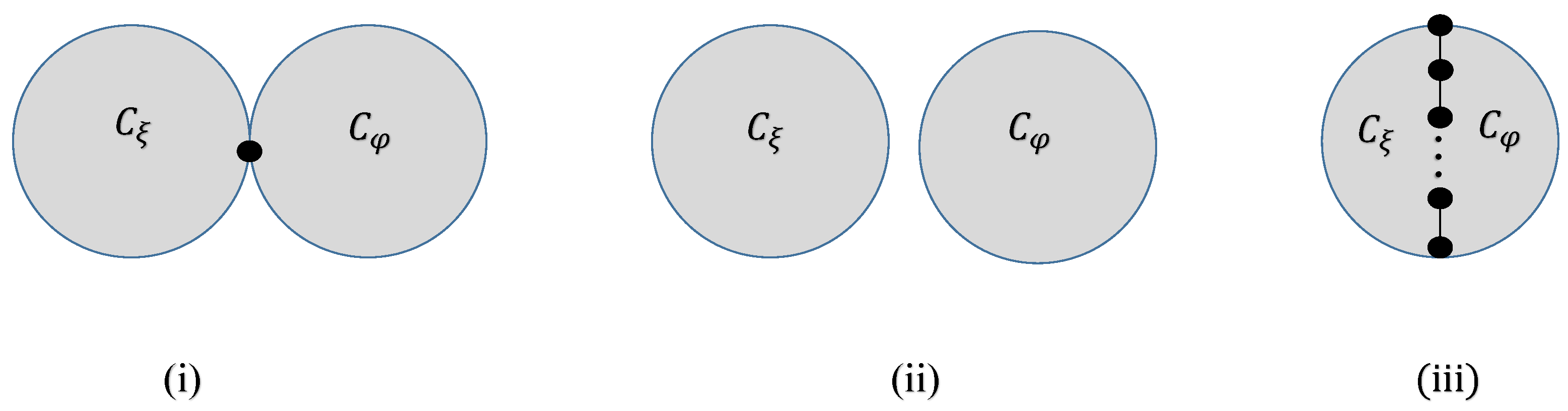
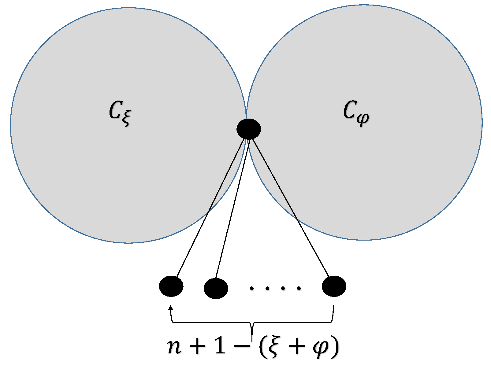
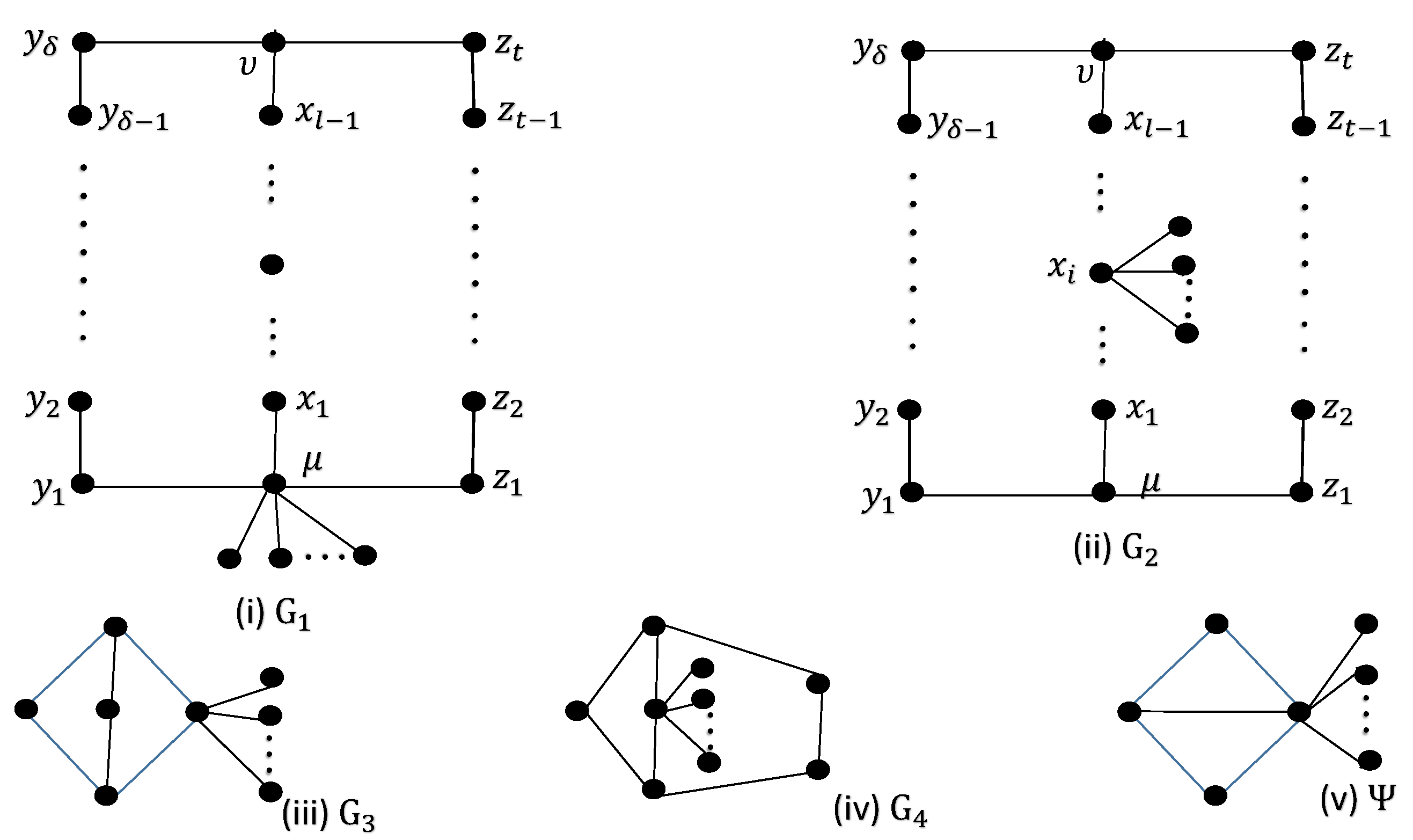
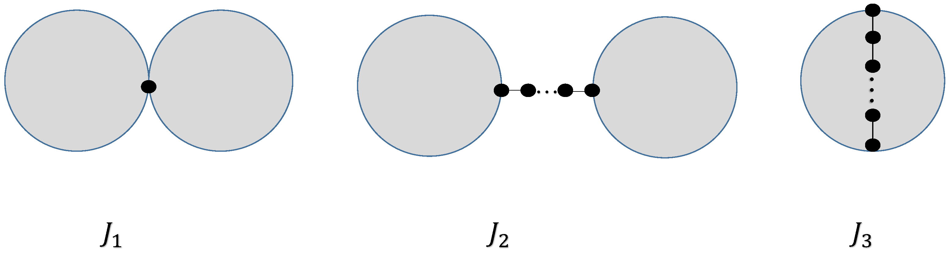
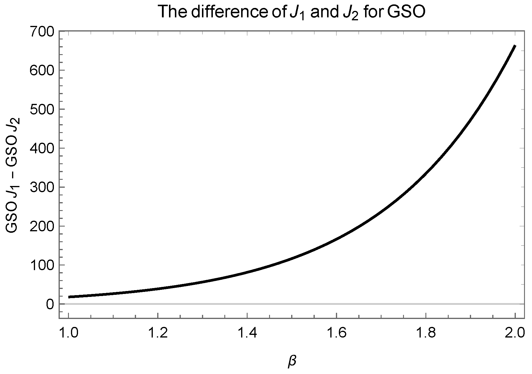
3. $\mathit{GSO}\mathbf{\left(}\mathit{G}\mathbf{\right)}$ for Greatest Values

Let $U_n^k$ be unicyclic graph obtained from $C_k$ in which $n-k$ pendent edges are attached to the same vertex on $C_k$, then using Lemmas 1 and 2, it follows that

Theorem 1. 

Consider G be an unicyclic graph with order n and girth k, if G is not $U_n^k$ then $GSO\left(G\right)<GSO\left({\mu }_n^k\right)$.

Consider bicyclic graph $G(n,n+1)$. Here the order is n, and the size is $n+1$. The considered bicyclic graph has been investigated for the Sombor index. We consider a connected and simple graph denoted by $\Theta (n,n+1)$. Furthermore, for $G\in \Theta (n,n+1)$, every graph consists of cycles $C_{\xi }$ and $C_{\phi }$ in G. The following cases have been observed;

(I)

$\mathbb{A}(\xi ,\phi )$ consists of $G\in \Theta (n,n+1)$, where $C_{\xi }$ and $C_{\phi }$ share one vertex in common.

(II)

$\mathbb{B}(\xi ,\phi )$ consists of $G\in \Theta (n,n+1)$, where $C_{\xi }$ and $C_{\phi }$ share no common vertex.

(III)

$\mathbb{C}(\xi ,\phi ,l)$ contains $G\in \Theta (n,n+1)$, where the cycles $C_{\xi }$ and $C_{\phi }$ are connected by a common path of length l.

In Figure 3i–iii, vertex induced subgraphs on the cycles for $G\in \mathbb{A}(\xi ,\phi )$ (or $\mathbb{B}(\xi ,\phi )$, $\mathbb{C}(\xi ,\phi ,l)$) are provided, respectively.

4. Greatest $\mathit{GSO}$ in the Family $\mathbb{A}(\mathit{\xi },\mathit{\phi })$

In this portion, we investigated $GSO$ in $\mathbb{A}(\xi ,\phi )$ for optimal values. Let $S_n(\xi ,\phi )$ be from $\mathbb{A}(\xi ,\phi )$ where $n-\xi +1-\phi$ pendent edges are attached directly to the common vertex of $C_{\xi }$ and $C_{\phi }$, for this we provide Figure 4.

Theorem 2. 

$S_n(\xi ,\phi )$ is the graph with greatest $GSO$ in $\mathbb{A}(\xi ,\phi )$.

Proof. 

Consider G and apply Transformation A and Transformation B. We obtain $G^{\prime }$ in which all the edges not on the cycle are connected directly to v. Using Lemmas 1 and 2, we obtain that $GSO\left(G^{\prime }\right)>GSO\left(G\right)$ with equality iff, all the non-cyclic edges are connected directly to the same vertex in G. If $G^{\prime }\ncong S_n(\xi ,\phi )$, then $\mu$ and v are different vertices and $\mu$ is vertex that is common between $C_{\phi }$ and $C_{\xi }$.

Consider that v is on the cycle $C_{\xi }$, we consider cases given below;

• Case 1. Consider that v and $\mu$ are not adjacent, the following is considered

  $$\begin{array}{cc}& GSO\left(S_n(\xi ,\phi )\right)={({(5-\xi -\phi +n)}^2+1)}^{\beta }+{({(5-\xi -\phi +n)}^2+1)}^{\beta }\hfill \\ & +\cdots +{({(5-\xi -\phi +n)}^2+1)}^{\beta }+4{({(5-\xi -\phi +n)}^2+4)}^{\beta }\hfill \\ & +(\xi -2){\left(8\right)}^{\beta }+(\phi -2){\left(8\right)}^{\beta },\hfill \\ & =(n-\xi +1-\phi ){({(5-\xi -\phi +n)}^2+1)}^{\beta }+4{({(5-\xi -\phi +n)}^2+4)}^{\beta }\hfill \\ & +(\xi -2)8^{\beta }+(\phi -2)8^{\beta }.\hfill \end{array}$$

  $GSO$ for $G^{\prime }$, is considered in the following

  $$\begin{array}{cc}& GSO\left(G^{\prime }\right)={({(3-\xi -\phi +n)}^2+1)}^{\beta }+{({(3-\xi -\phi +n)}^2+1)}^{\beta }\hfill \\ & +\cdots +{({(3-\xi -\phi +n)}^2+1)}^{\beta }+2{({(3-\xi -\phi +n)}^2+4)}^{\beta }\hfill \\ & +(\xi -4){\left(8\right)}^{\beta }+(\phi -2){\left(8\right)}^{\beta }+4{\left(20\right)}^{\beta },\hfill \\ & =(n-\xi +1-\phi ){({(3-\xi -\phi +n)}^2+1)}^{\beta }+2{({(3-\xi -\phi +n)}^2+4)}^{\beta }\hfill \\ & +(\xi -4)8^{\beta }+(\phi -2)8^{\beta }+4{\left(20\right)}^{\beta }.\hfill \end{array}$$

  Consider the following difference

  $$\begin{array}{cc}& GSO\left(S_n(\xi ,\phi )\right)-GSO\left(G^{\prime }\right)=(n-\xi +1-\phi ){({(5-\xi -\phi +n)}^2+1)}^{\beta }+4{({(5-\xi -\phi +n)}^2+4)}^{\beta }\hfill \\ & +(\xi -2)8^{\beta }-(n-\xi +1-\phi ){({(3-\xi -\phi +n)}^2+1)}^{\beta }-2{({(3-\xi -\phi +n)}^2+4)}^{\beta }\hfill \\ & -(\xi -4)8^{\beta }-4{\left(20\right)}^{\beta },\hfill \\ & =(n-\xi +1-\phi ){({(5-\xi -\phi +n)}^2+1)}^{\beta }+2{({(5-\xi -\phi +n)}^2+4)}^{\beta }\hfill \\ & +(\xi -2)8^{\beta }+2{({(5-\xi -\phi +n)}^2+4)}^{\beta }-(n-\xi +1-\phi ){({(3-\xi -\phi +n)}^2+1)}^{\beta }\hfill \\ & -2{({(3-\xi -\phi +n)}^2+4)}^{\beta }-(\xi -4)8^{\beta }-4{\left(20\right)}^{\beta }>0.\hfill \end{array}$$

  (16)

  Here, equality holds iff $G^{\prime }\cong S_n(\xi ,\phi )$.
• Case 2. Consider that v and $\mu$ are connected directly by an edge in $G^{\prime }$. Then,

  $$\begin{array}{cc}& GSO\left(G^{\prime }\right)={({(3-\xi -\phi +n)}^2+1^1)}^{\beta }+{({(3-\xi -\phi +n)}^2+1^1)}^{\beta }\hfill \\ & +\cdots +{({(3-\xi -\phi +3)}^2+1^1)}^{\beta }+{({(3-\xi -\phi +n)}^2+{\left(2\right)}^2)}^{\beta }\hfill \\ & +{({(n+3-\xi -\phi )}^2+4^2)}^{\beta }+3(4^2+{\left(2\right)}^2)+(\xi -3){({\left(2\right)}^2+{\left(2\right)}^2)}^{\beta }+(\phi -2){({\left(2\right)}^2+{\left(2\right)}^2)}^{\beta },\hfill \\ & =(n-\xi +1-\phi ){({(n+3-\xi -\phi )}^2+1)}^{\beta }+{({(n+3-\xi -\phi )}^2+4)}^{\beta }\hfill \\ & +{({(n+3-\xi -\phi )}^2+16)}^{\beta }+3{\left(20\right)}^{\beta }+(\xi -3)8^{\beta }+(\phi -2)8^{\beta }.\hfill \end{array}$$

  (17)

  The following difference is considered

  $$\begin{array}{cc}& GSO\left(S_n(\xi ,\phi )\right)-GSO\left(G^{\prime }\right)=(n-\xi +1-\phi ){({(5-\xi -\phi +n)}^2+1)}^{\beta }+4{({(5-\xi -\phi +n)}^2+4)}^{\beta }\hfill \\ & +(\xi -2)8^{\beta }+(\phi -2)8^{\beta }\hfill \\ & -(n-\xi +1-\phi ){({(3-\xi -\phi +n)}^2+1)}^{\beta }-{({(3-\xi -\phi +n)}^2+4)}^{\beta }\hfill \\ & -{({(n+3-\xi -\phi )}^2+16)}^{\beta }-3{\left(20\right)}^{\beta }-(\xi -3)8^{\beta }-(\phi -2)8^{\beta },\hfill \\ & =(n-\xi +1-\phi ){({(5-\xi -\phi +n)}^2+1)}^{\beta }+{({(5-\xi -\phi +n)}^2+4)}^{\beta }\hfill \\ & +2{({(5-\xi -\phi +n)}^2+4)}^{\beta }+(\xi -2)8^{\beta }+{({(5-\xi -\phi +n)}^2+4)}^{\beta }\hfill \\ & -(n-\xi +1-\phi ){({(3-\xi -\phi +n)}^2+1)}^{\beta }-{({(3-\xi -\phi +n)}^2+4)}^{\beta }\hfill \\ & -{({(3-\xi -\phi +n)}^2+16)}^{\beta }-(\xi -3)8^{\beta }-3{\left(20\right)}^{\beta }>0.\hfill \end{array}$$

  (18)

  While equality holds iff $G^{\prime }\cong S_n(\xi ,\phi )$.

□

For $3\le \xi$ and $3\le \phi$, applying above theorem, it follows that $S_n(\xi ,\phi )$ is the unique graph with largest value for $GSO$ in $\mathbb{A}(\xi ,\phi )$.

Lemma 3. 

(i) For $3<\xi$ we have $GSO\left(S_n(\xi -1,\phi )\right)>GSO\left(S_n(\xi ,\phi )\right)$; (ii) For $3<\phi$, we have $GSO\left(S_n(\xi ,\phi -1)\right)>GSO\left(S_n(\xi ,\phi )\right)$.

Proof. 

(i) As we have

$$\begin{array}{cc}& GSO\left(S_n(\xi ,\phi )\right)=(1-\xi -\phi +n){({(5-\xi -\phi +n)}^2+1)}^{\beta }+4{({(5-\xi -\phi +n)}^2+4)}^{\beta }\hfill \\ & +(\xi -2)8^{\beta }+(\phi -2)8^{\beta }.\hfill \end{array}$$

Plug $\xi$ by $\xi -1$, it follows that

$$\begin{array}{cc}& GSO\left(S_n(\xi -1,\phi )\right)=(2-\xi -\phi +n){({(5-\xi +1-\phi +n)}^2+1)}^{\beta }\hfill \\ & +4{({(5-\xi +1-\phi +n)}^2+4)}^{\beta }+(\xi -1-2)8^{\beta }+(\phi -2)8^{\beta },\hfill \\ & =(2-\xi -\phi +n){({(6-\xi -\phi +n)}^2+1)}^{\beta }\hfill \\ & +4{({(6-\xi -\phi +n)}^2+4)}^{\beta }+(\xi -3)8^{\beta }+(\phi -2)8^{\beta }.\hfill \end{array}$$

From the above calculations, the following difference is considered

$$\begin{array}{cc}& GSO\left(S_n(\xi -1,\phi )\right)-GSO\left(S_n(\xi ,\phi )\right)=(2-\xi -\phi +n){({(6-\xi -\phi +n)}^2+1)}^{\beta }\hfill \\ & +4{({(6-\xi -\phi +n)}^2+4)}^{\beta }+(\xi -3)8^{\beta }\hfill \\ & -(n-\xi +1-\phi ){({(5-\xi -\phi +n)}^2+1)}^{\beta }-4{({(5-\xi -\phi +n)}^2+4)}^{\beta }\hfill \\ & -(\xi -2)8^{\beta }>0.\hfill \end{array}$$

Hence, we have $GSO\left(S_n(\xi -1,\phi )\right)>GSO\left(S_n(\xi ,\phi )\right)$.

Consider (ii). We have the following:

$$\begin{array}{cc}& GSO\left(S_n(\xi ,\phi -1)\right)-GSO\left(S_n(\xi ,\phi )\right)=(2-\xi -\phi +n){({(6-\xi -\phi +n)}^2+1)}^{\beta }\hfill \\ & +4{({(6-\xi -\phi +n)}^2+4)}^{\beta }+(\phi -3)8^{\beta }\hfill \\ & -(n-\xi +1-\phi ){({(5-\xi -\phi +n)}^2+1)}^{\beta }-4{({(5-\xi -\phi +n)}^2+4)}^{\beta }-(\phi -2)8^{\beta }>0.\hfill \end{array}$$

Finally, we have $GSO\left(S_n(\xi ,\phi -1)\right)>GSO\left(S_n(\xi ,\phi )\right)$. □

From Theorem 2 and Lemma 3, we obtain the following:

Theorem 3. 

For every $\xi \ge 3$ and $\phi \ge 3$, the unique graph of order n with largest value of $GSO$ is $S_n(3,3)$ in $\mathbb{A}(\xi ,\phi )$.

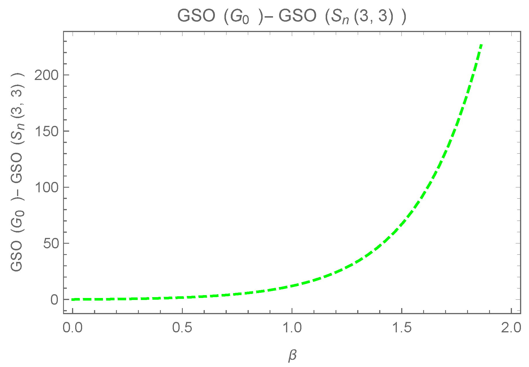
5. $\mathit{GSO}$ for Greatest Values in $\mathbb{B}\mathbf{(}\mathit{\xi }\mathbf{,}\mathit{\phi }\mathbf{)}$

In the considered portion, the largest values in bicyclic graphs of $GSO$ are considered in $\mathbb{B}(\xi ,\phi )$. Let $T_n^{\delta }(\xi ,\phi )$ be the graph on n vertices and $n+1$ edges. Two cycles $C_{\xi }$ and $C_{\phi }$ are connected by a path of length $\delta$. Here, $n-\delta -\xi +1-\phi$ pendent edges are connected directly to the common vertex of cycle $C_{\xi }$ and the path. We provide Figure 5a, and $T_n^r((\phi ,\xi )$ is given in Figure 5b. $T_n(\xi ,\phi )$ is the graph on $n+1$ edges and n vertices, obtained by connecting $C_{\xi }$ and $C_{\phi }$ by a path $\mu vw$, the remaining edges are connected directly to v; see Figure 5c.

Theorem 4. 

Let $G\in \mathbb{B}(\xi ,\phi )$. Consider a common path of length δ of $C_{\xi }$ and $C_{\phi }$, then

$$\begin{array}{cc}& GSO\left(T_n^{\delta }(\xi ,\phi )\right)\ge GSO\left(G\right)\mathit{with} \mathit{holds} \mathit{iff} \mathrm{G}\cong T_n^{\delta }(\xi ,\phi ),\hfill \\ & GSO\left(T_n^{\delta }(\phi ,\xi )\right)\ge GSO\left(G\right)\mathit{with} \mathit{equality} \mathit{iff} \mathrm{G}\cong T_n^{\delta }(\phi ,\xi ).\hfill \end{array}$$

(19)

Proof. 

Consider a path of shortest length denoted by $P=v_1{v}_2\cdots v_{\delta }{v}_{\delta +1}$, the considered path connects $C_{\xi }$ and $C_{\phi }$ in G. Let $v_1$ be the common vertex between P and $C_{\xi }$, $v_{\delta +1}$ be the common vertex of P and $C_{\phi }$. Using Transformation A and Transformation B on G continuously, we obtain $G^{\prime }$ as provided in Figure 5. In $G^{\prime }$, all the vertices of degree one not on the cycles are connected directly to vertex v. Applying Lemmas 1 and 2, we obtain $GSO\left(G^{\prime }\right)>GSO\left(G\right)$, with equality iff all the edges not on the cycles are pendent edges connected directly to the same vertex in G. We consider the cases given below.

• Case 1. If v is on $C_{\xi }$ with adjacent v and $v_1$, we provided Figure 5d. Here, the following values are considered

  $$\begin{array}{cc}& GSO\left(G^{\prime }\right)={({(n-\delta -\xi +3-\phi )}^2+1)}^{\beta }+\cdots +{({(n-\delta -\xi +3-\phi )}^2+1)}^{\beta }\hfill \\ & +2{({(n-\delta -\xi +3-\phi )}^2+2^2)}^{\beta }+{(9+d{\left(v_2\right)}^2)}^{\beta }+(\xi -4){\left(8\right)}^{\beta }\hfill \\ & +(\phi -2){\left(8\right)}^{\beta }+(\delta -2){\left(8\right)}^{\beta }+3{\left(11\right)}^{\beta }+2{\left(11\right)}^{\beta },\hfill \\ & =(n-\delta -\xi +1-\phi ){({(n-\delta -\xi +3-\phi )}^2+1)}^{\beta }+2{({(n-\delta -\xi +3-\phi )}^2+4)}^{\beta }\hfill \\ & +{(9+d{\left(v_2\right)}^2)}^{\beta }+8^{\beta }(\xi -4)+8^{\beta }(\phi -2)+8^{\beta }(\delta -2)+5{\left(13\right)}^{\beta }.\hfill \end{array}$$

  (20)

  $GSO\left(T_n^r(\xi ,\phi )\right)$ is given by

  $$\begin{array}{cc}& GSO\left(T_n^r(\xi ,\phi )\right)=(n-\delta -\xi +1-\phi ){({(n-\delta -\xi +4-\phi )}^2+1)}^{\beta }\hfill \\ & +2{({(n-\delta -\xi +4-\phi )}^2+4)}^{\beta }+{({(n-\delta -\xi +4-\phi )}^2+d{\left(v_2\right)}^2)}^{\beta }\hfill \\ & +(\delta -2){\left(8\right)}^{\beta }+(\xi -2){\left(8\right)}^{\beta }+(\phi -2){\left(8\right)}^{\beta }+3{\left(11\right)}^{\beta },\hfill \\ & =(n-\delta -\xi +1-\phi ){({(n-\delta -\xi +4-\phi )}^2+1)}^{\beta }\hfill \\ & +2{({(n-\delta -\xi +4-\phi )}^2+4)}^{\beta }+{({(n-\delta -\xi +4-\phi )}^2+d{\left(v_2\right)}^2)}^{\beta }\hfill \\ & +8^{\beta }(\delta -2)+8^{\beta }(\xi -2)+8^{\beta }(\phi -2)+3{\left(13\right)}^{\beta }.\hfill \end{array}$$

  (21)

  $GSO\left(T_n^r(\xi ,\phi )\right)-GSO\left(G^{\prime }\right)$, is considered in the following:

  $$\begin{array}{cc}& GSO\left(T_n^r(\xi ,\phi )\right)-GSO\left(G^{\prime }\right)=(n-\delta -\xi +1-\phi ){({(n-\delta -\xi +4-\phi )}^2+1)}^{\beta }+\hfill \\ & +2{({(n-\delta -\xi +4-\phi )}^2+4)}^{\beta }+{({(n-\delta -\xi +4-\phi )}^2+d{\left(v_2\right)}^2)}^{\beta }\hfill \\ & +8^{\beta }(\delta -2)+8^{\beta }(\xi -2)+8^{\beta }(\phi -2)+3{\left(13\right)}^{\beta }\hfill \\ & -(n-\delta -\xi +1-\phi ){({(n-\delta -\xi +3-\phi )}^2+1)}^{\beta }-2{({(n-\delta -\xi +3-\phi )}^2+4)}^{\beta }\hfill \\ & -{(9+d{\left(v_2\right)}^2)}^{\beta }-8^{\beta }(\xi -4)-8^{\beta }(\phi -2)-8^{\beta }(\delta -2)-5{\left(13\right)}^{\beta },\hfill \\ & =(n-\delta -\xi +1-\phi ){({(n-\delta -\xi +4-\phi )}^2+1)}^{\beta }\hfill \\ & +2{({(n-\delta -\xi +4-\phi )}^2+4)}^{\beta }+{({(n-\delta -\xi +4-\phi )}^2+d{\left(v_2\right)}^2)}^{\beta }\hfill \\ & -(n-\delta -\xi +1-\phi ){({(n-\delta -\xi +3-\phi )}^2+1)}^{\beta }-2{({(n-\delta -\xi +3-\phi )}^2+4)}^{\beta }\hfill \\ & -{(9+d{\left(v_2\right)}^2)}^{\beta }+8^{\beta }(\xi -2)+3{\left(13\right)}^{\beta }-8^{\beta }(\xi -4)-5{\left(13\right)}^{\beta }\ge 0.\hfill \end{array}$$

  (22)

  Hence, $GSO\left(T_n^{\delta }(\xi ,\phi )\right)-GSO\left(G^{\prime }\right)>0$, with equality iff $G^{\prime }\cong T_n^{\delta }(\xi ,\phi )$, Figure 6 is provided for equality.
• If the vertices $v_1$ and v are directly connected by an edge in $G^{\prime }$, we provide the values in the following

  $$\begin{array}{cc}& GSO\left(G^{\prime }\right)={({(n-\delta -\xi +3-\phi )}^2+1)}^{\beta }+\cdots +{({(n-\delta -\xi +3-\phi )}^2+1)}^{\beta }\hfill \\ & +{({(n-\delta -\xi +3-\phi )}^2+4)}^{\beta }+{({(n-\delta -\xi +3-\phi )}^2+9)}^{\beta }\hfill \\ & +{(9+d{\left(v_2\right)}^2)}^{\beta }+4{\left(11\right)}^{\beta }+(\xi -3){\left(8\right)}^{\beta }+(\phi -2){\left(8\right)}^{\beta }+(\delta -2){\left(8\right)}^{\beta },\hfill \\ & =(n-\delta -\xi +1-\phi ){({(n-\delta -\xi +3-\phi )}^2+1)}^{\beta }+{({(n-\delta -\xi +3-\phi )}^2+4)}^{\beta }\hfill \\ & +{({(n-\delta -\xi +3-\phi )}^2+27)}^{\beta }+{(9+d{\left(v_2\right)}^2)}^{\beta }+4{\left(31\right)}^{\beta }+(\xi -3)8^{\beta }\hfill \\ & +(\phi -2)8^{\beta }+(\delta -2)8^{\beta }.\hfill \end{array}$$

  (23)

  Next, we consider $GSO\left(T_n^{\delta }(\xi ,\phi )\right)-GSO\left(G^{\prime }\right)$ in the following

  $$\begin{array}{cc}& GSO\left(T_n^r(\xi ,\phi )\right)-GSO\left(G^{\prime }\right)=(n-\delta -\xi +1-\phi ){({(n-\delta -\xi +4-\phi )}^2+1)}^{\beta }\hfill \\ & +{({(n-\delta -\xi +4-\phi )}^2+4)}^{\beta }+{({(n-\delta -\xi +4-\phi )}^2+4)}^{\beta }\hfill \\ & +{({(n-\delta -\xi +4-\phi )}^2+d{\left(v_2\right)}^2)}^{\beta }+8^{\beta }(\delta -2)+8^{\beta }(\xi -2)+8^{\beta }(\phi -2)+3{\left(13\right)}^{\beta }\hfill \\ & -(n-\delta -\xi +1-\phi ){({(n-\delta -\xi +3-\phi )}^2+1)}^{\beta }-{({(n-\delta -\xi +3-\phi )}^2+4)}^{\beta }\hfill \\ & -{({(n-\delta -\xi +3-\phi )}^2+27)}^{\beta }-{(9+d{\left(v_2\right)}^2)}^{\beta }-(\xi -3)8^{\beta }-(\phi -2)8^{\beta }-(\delta -2)8^{\beta }-4{\left(13\right)}^{\beta },\hfill \\ & =(n-\delta -\xi +1-\phi ){({(n-\delta -\xi +4-\phi )}^2+1)}^{\beta }\hfill \\ & +{({(n-\delta -\xi +4-\phi )}^2+4)}^{\beta }+{({(n-\delta -\xi +4-\phi )}^2+4)}^{\beta }\hfill \\ & +{({(n-\delta -\xi +4-\phi )}^2+d{\left(v_2\right)}^2)}^{\beta }+8^{\beta }(\xi -2)+3{\left(13\right)}^{\beta }\hfill \\ & -(n-\delta -\xi +1-\phi ){({(n-\delta -\xi +3-\phi )}^2+1)}^{\beta }-{({(n-\delta -\xi +3-\phi )}^2+4)}^{\beta }\hfill \\ & -{({(n-\delta -\xi +3-\phi )}^2+9)}^{\beta }-{(9+d{\left(v_2\right)}^2)}^{\beta }-(\xi -3)8^{\beta }-4{\left(13\right)}^{\beta }.\hfill \end{array}$$

  (24)

  Hence, we have $GSO\left(T_n^{\delta }(\xi ,\phi )\right)-GSO\left(G^{\prime }\right)>0$, with equality iff $G^{\prime }\cong \left(T_n^{\delta }(\xi ,\phi )\right)$. Figure 7 is provided for this.
• Case 2. Consider v on $C_{\phi }$, this case is similar to Case 1. Figure 5e is provided for Case 2.
• Case 3. Consider v on P as in Figure 5f, when $G^{\prime }\ncong T_n(\xi ,\phi )$, then $\delta \ge 3$. The following is considered;
  When $\delta >t>2$, then $\delta >3$ and the following value is considered

  $$\begin{array}{cc}& GSO\left(T_n(\xi ,\phi )\right)={({(n-\xi +1-\phi +)}^2+1)}^{\beta }+\cdots +{({(n-\xi +1-\phi )}^2+1)}^{\beta }\hfill \\ & +2{({(n-\xi +1-\phi )}^2+9)}^{\beta }+4{\left(11\right)}^{\beta }+(\xi -2){\left(8\right)}^{\beta }+(\phi -2){\left(8\right)}^{\beta },\hfill \\ & =(n-\xi -1-\phi ){({(n-\xi +1-\phi )}^2+1)}^{\beta }+2{({(n-\xi +1-\phi )}^2+9)}^{\beta }\hfill \\ & +4{\left(13\right)}^{\beta }+(\xi -2)8^{\beta }+(\phi -2)8^{\beta }.\hfill \end{array}$$

  (25)

  $GSO$ for $G^{\prime }$ is considered in the following:

  $$\begin{array}{cc}& GSO\left(G^{\prime }\right)={({(n-\delta -\xi +1-\phi )}^2+1)}^{\beta }+\cdots +{({(n-\delta -\xi +1-\phi )}^2+1)}^{\beta }\hfill \\ & +2{({(n-\delta -\xi +1-\phi )}^2+4)}^{\beta }+(\xi -2){\left(8\right)}^{\beta }+(\phi -2){\left(8\right)}^{\beta }\hfill \\ & +(\delta -4){\left(8\right)}^{\beta }+6\left(11\right),\hfill \\ & =(n-\delta -\xi +1-\phi ){({(n-\delta -\xi +1-\phi )}^2+1)}^{\beta }+2{({(n-\delta -\xi +1-\phi )}^2+4)}^{\beta }\hfill \\ & +(\xi -2)8^{\beta }+(\phi -2)8^{\beta }+(\delta -4)8^{\beta }+6{\left(31\right)}^{\beta }.\hfill \end{array}$$

  (26)

  We consider the difference of $GSO\left(T_n(\xi ,\phi )\right)$ and $GSO\left(G^{\prime }\right)$ in the following

  $$\begin{array}{cc}& GSO\left(T_n(\xi ,\phi )\right)-GSO\left(G^{\prime }\right)=(n-\xi -1-\phi ){({(n-\xi +1-\phi )}^2+1)}^{\beta }\hfill \\ & +2{({(n-\xi +1-\phi )}^2+9)}^{\beta }+(\xi -2)8^{\beta }+(\phi -2)8^{\beta }+4{\left(13\right)}^{\beta }\hfill \\ & -(n-\delta -\xi +1-\phi ){({(n-\delta -\xi +1-\phi )}^2+1)}^{\beta }-2{({(n-\delta -\xi +1-\phi )}^2+4)}^{\beta }\hfill \\ & -(\xi -2)8^{\beta }-(\phi -2)8^{\beta }-(\delta -4)8^{\beta }-6{\left(13\right)}^{\beta },\hfill \\ & =(n-\xi -1-\phi ){({(n-\xi +1-\phi )}^2+1)}^{\beta }+2{({(n-\xi +1-\phi )}^2+9)}^{\beta }+4{\left(13\right)}^{\beta }\hfill \\ & -(n-\delta -\xi +1-\phi ){({(n-\delta -\xi +1-\phi )}^2+1)}^{\beta }-2{({(n-\delta -\xi +1-\phi )}^2+4)}^{\beta }\hfill \\ & -(\delta -4)8^{\beta }-6{\left(13\right)}^{\beta }.\hfill \end{array}$$

  (27)

  Figure 8 is provided for the difference in Equation (27).
  If $2=t$ or $t=\delta$, then for $G^{\prime }$ the value of $GSO$ is considered in the following

  $$\begin{array}{cc}& GSO\left(G^{\prime }\right)=5{\left(11\right)}^{\beta }+(\xi -2){\left(8\right)}^{\beta }+(\phi -2){\left(8\right)}^{\beta }\hfill \\ & +{(9+{(n-\delta -\xi +3-\phi )}^2)}^{\beta }+{(4+{(n-\delta -\xi +3-\phi )}^2)}^{\beta }+\hfill \\ & {({(n-\delta -\xi +3-\phi )}^2+1)}^{\beta }+\cdots +{({(n-\delta -\xi +3-\phi )}^2+1)}^{\beta }+(\delta -3){\left(8\right)}^{\beta },\hfill \\ & =(\xi -2){\left(8\right)}^{\beta }+(\phi -2){\left(8\right)}^{\beta }+{(9+{(n-\delta -\xi +3-\phi )}^2)}^{\beta }+(\delta -3){\left(8\right)}^{\beta }\hfill \\ & +{(4+{(n-\delta -\xi +3-\phi )}^2)}^{\beta }+(n-\delta -\xi +1-\phi ){({(n-\delta -\xi +3-\phi )}^2+1)}^{\beta }\hfill \\ & +5{\left(13\right)}^{\beta }>0.\hfill \end{array}$$

  (28)

  The difference of $GSO\left(T_n(\xi ,\phi )\right)$ and $GSO\left(G^{\prime }\right)$ is in the following

  $$\begin{array}{cc}& GSO\left(T_n(\xi ,\phi )\right)-GSO\left(G^{\prime }\right)=(n-\xi -1-\phi ){({(n-\xi +1-\phi )}^2+1)}^{\beta }\hfill \\ & +2{({(n-\xi +1-\phi )}^2+9)}^{\beta }+(\xi -2)8^{\beta }+(\phi -2)8^{\beta }+4{\left(13\right)}^{\beta }\hfill \\ & -{(9+{(n-\delta -\xi +3-\phi )}^2)}^{\beta }-{(4+{(n-\delta -\xi +3-\phi )}^2)}^{\beta }\hfill \\ & -(n-\delta -\xi +1-\phi ){({(n-\delta -\xi +3-\phi )}^2+1)}^{\beta }-(\xi -2)8^{\beta }-(\phi -2)8^{\beta }\hfill \\ & -(\delta -3)8^{\beta }-5{\left(13\right)}^{\beta },\hfill \\ & =(n-\xi -1-\phi ){({(n-\xi +1-\phi )}^2+1)}^{\beta }+2{({(n-\xi +1-\phi )}^2+9)}^{\beta }\hfill \\ & -{(9+{(n-\delta -\xi +3-\phi )}^2)}^{\beta }-{(4+{(n-\delta -\xi +3-\phi )}^2)}^{\beta }\hfill \\ & -(n-\delta -\xi +1-\phi ){({(n-\delta -\xi +3-\phi )}^2+1)}^{\beta }-(\delta -3)8^{\beta }-{\left(13\right)}^{\beta },\hfill \\ & >0.\hfill \end{array}$$

  (29)

  Figure 9 is provided for the difference in the Equation (29).

□

Lemma 4. 

$GSO\left(T_n(3,3)\right)\ge GSO\left(T_n(\xi ,\phi )\right)$, with equality iff $\xi =3=\phi$.

Proof. 

The previous theorem provided the following value:

$$\begin{array}{cc}& GSO\left(T_n(\xi ,\phi )\right)=(n-\xi -1-\phi ){({(n-\xi +1-\phi )}^2+1)}^{\beta }+2{({(n-\xi +1-\phi )}^2+9)}^{\beta }\hfill \\ & +4{\left(13\right)}^{\beta }+(\xi -2)8^{\beta }+(\phi -2)8^{\beta }.\hfill \end{array}$$

(30)

For $GSO\left(T_n(3,3)\right)$, the following is considered

$$\begin{array}{cc}& GSO\left(T_n(3,3)\right)=4{\left(11\right)}^{\beta }+2{\left(8\right)}^{\beta }+2{(9+{(n-5)}^2)}^{\beta }+(n-7){(1+{(n-5)}^2)}^{\beta },\hfill \\ & =4{\left(13\right)}^{\beta }+2{\left(8\right)}^{\beta }+2{(1+{(n-5)}^2)}^{\beta }+(n-7){(1+{(n-5)}^2)}^{\beta }.\hfill \end{array}$$

(31)

Furthermore, we have the following difference:

$$\begin{array}{cc}& GSO\left(T_n(3,3)\right)-GSO\left(T_n(\xi ,\phi )\right)=2{\left(8\right)}^{\beta }+2{(9+{(n-5)}^2)}^{\beta }+(n-7){(1+{(n-5)}^2)}^{\beta }\hfill \\ & -(n-\xi -1-\phi ){({(n-\xi +1-\phi )}^2+1)}^{\beta }+2{({(n-\xi +1-\phi )}^2+9)}^{\beta }\hfill \\ & +(\xi -2)8^{\beta }+(\phi -2)8^{\beta }\ge 0.\hfill \end{array}$$

(32)

Figure 10 is provided for the difference in Equation (32), with iff $\xi =3=\phi$. For equality, Figure 11 is provided. □

Lemma 5. 

For $2\le \delta$, $GSO\left(T_n^{\delta -1}(\xi ,\phi )\right)>GSO\left(T_n^{\delta }(\xi ,\phi )\right)$.

Proof. 

For the proof, we consider the following:

If $\delta >2$, then $GSO\left(T_n^{\delta }(\xi ,\phi )\right)$, is considered in the following

$$\begin{array}{cc}& GSO\left(T_n^{\delta }(\xi ,\phi )\right)=(n-\delta -\xi +1-\phi ){({(n-\delta -\xi +4-\phi )}^2+1)}^{\beta }\hfill \\ & +2{({(n-\delta -\xi +4-\phi )}^2+4)}^{\beta }+{({(n-\delta -\xi +4-\phi )}^2+d{\left(v_2\right)}^2)}^{\beta }\hfill \\ & +8^{\beta }(\delta -2)+8^{\beta }(\xi -2)+3{\left(13\right)}^{\beta }+8^{\beta }(\phi -2).\hfill \end{array}$$

Here, $d\left(v_2\right)=2$, it follows that

$$\begin{array}{cc}& GSO\left(T_n^{\delta }(\xi ,\phi )\right)=(n-\delta -\xi +1-\phi ){({(n-\delta -\xi +4-\phi )}^2+1)}^{\beta }\hfill \\ & +2{({(n-\delta -\xi +4-\phi )}^2+4)}^{\beta }+{({(n-\delta -\xi +4-\phi )}^2+4)}^{\beta }\hfill \\ & +8^{\beta }(\delta -2)+8^{\beta }(\xi -2)+8^{\beta }(\phi -2)+3{\left(13\right)}^{\beta }.\hfill \end{array}$$

(33)

Replacing $\delta$ by $\delta -1$ in (33), it follows that

$$\begin{array}{cc}& GSO\left(T_n^{\delta -1}(\xi ,\phi )\right)=(2-\xi -\phi -\delta +n){({(5-\xi -\phi +n-\delta )}^2+1)}^{\beta }\hfill \\ & +2{({(5-\xi -\phi -\delta +n)}^2+4)}^{\beta }+{({(5-\xi -\phi +n-\delta )}^2+4)}^{\beta }\hfill \\ & +8^{\beta }(\delta -3)+8^{\beta }(\xi -2)+8^{\beta }(\phi -2)+3{\left(13\right)}^{\beta }.\hfill \end{array}$$

The difference of $GSO\left(T_n^{\delta }(\xi ,\phi )\right)$ and $GSO\left(T_n^{\delta -1}(\xi ,\phi )\right)$ is considered in the following

$$\begin{array}{cc}& GSO\left(T_n^{\delta -1}(\xi ,\phi )\right)-GSO\left(T_n^r(\xi ,\phi )\right)=(n+2-\xi -\phi -\delta ){({(5-\xi -\phi +n-\delta )}^2+1)}^{\beta }\hfill \\ & +2{({(5-\xi -\phi +n-\delta )}^2+4)}^{\beta }+{({(5-\xi -\phi +n-\delta )}^2+4)}^{\beta }\hfill \\ & +8^{\beta }(\delta -3)+8^{\beta }(\xi -2)+8^{\beta }(\phi -2)+3{\left(13\right)}^{\beta }\hfill \\ & -(n-\delta -\xi +1-\phi ){({(n-\delta -\xi +4-\phi )}^2+1)}^{\beta }\hfill \\ & -2{({(n-\delta -\xi +4-\phi )}^2+4)}^{\beta }-{({(n-\delta -\xi +4-\phi )}^2+4)}^{\beta }\hfill \\ & -8^{\beta }(\delta -2)-8^{\beta }(\xi -2)-8^{\beta }(\phi -2)-3{\left(13\right)}^{\beta }.\hfill \end{array}$$

The difference $GSO\left(T_n^{\delta -1}(\xi ,\phi )\right)-GSO\left(T_n^{\delta }(\xi ,\phi )\right)>0$ is observed in Figure 12.

If $\delta =2$, then the following is considered

$$\begin{array}{cc}& GSO\left(T_n^{\delta }(\xi ,\phi )\right)=(n-\xi -1-\phi ){({(2-\xi -\phi +n)}^2+1)}^{\beta }\hfill \\ & +2{({(2-\xi -\phi +n)}^2+4)}^{\beta }+{({(2-\xi -\phi +n)}^2+4)}^{\beta }\hfill \\ & +8^{\beta }(2-2)+8^{\beta }(\xi -2)+8^{\beta }(\phi -2)+3{\left(13\right)}^{\beta }.\hfill \end{array}$$

For $GSO\left(T_n^{\delta -1}(\xi ,\phi )\right)$, it follows that

$$\begin{array}{cc}& GSO\left(T_n^{\delta -1}(\xi ,\phi )\right)=(n-\xi -\phi ){(1+{(3-\xi -\phi +n)}^2)}^{\beta }+2{(4+{(3-\xi -\phi +n)}^2)}^{\beta }\hfill \\ & +{(9+{(3-\xi -\phi +n)}^2)}^{\beta }+(\xi -2){\left(8\right)}^{\beta }+(\phi -2){\left(8\right)}^{\beta }+2{\left(11\right)}^{\beta },\hfill \\ & =(n-\xi -\phi ){({(n-\xi -\phi +3)}^2+1)}^{\beta }+2{({(3-\xi -\phi +n)}^2+4)}^{\beta }\hfill \\ & +{({(3-\xi -\phi +n)}^2+9)}^{\beta }+(\xi -2){\left(8\right)}^{\beta }+(\phi -2){\left(8\right)}^{\beta }+2{\left(13\right)}^{\beta }.\hfill \end{array}$$

Consider $GSO\left(T_n^{\delta -1}(\xi ,\phi )\right)-GSO\left(T_n^{\delta }(\xi ,\phi )\right)$ in the following

$$\begin{array}{cc}& GSO\left(T_n^{r-1}(\xi ,\phi )\right)-GSO\left(T_n^r(\xi ,\phi )\right)=(n-\xi -\phi ){(1+{(3-\xi -\phi +n)}^2)}^{\beta }\hfill \\ & +2{(4+{(3-\xi -\phi +n)}^2)}^{\beta }+{(9+{(3-\xi -\phi +n)}^2)}^{\beta }\hfill \\ & +(\xi -2){\left(8\right)}^{\beta }+(\phi -2){\left(8\right)}^{\beta }+2{\left(13\right)}^{\beta }-(n-\xi -1-\phi ){({(2-\xi -\phi +n)}^2+1)}^{\beta }\hfill \\ & -2{({(2-\xi -\phi +n)}^2+4)}^{\beta }-{({(n+2-\xi -\phi )}^2+4)}^{\beta }\hfill \\ & -8^{\beta }(2-2)-8^{\beta }(\xi -2)-8^{\beta }(\phi -2)-3{\left(13\right)}^{\beta }\hfill \\ & >0.\hfill \end{array}$$

(34)

Figure 13 is provided for the difference in Equation (34). □

Lemma 6. 

$GSO\left(T_n^1(3,3)\right)\ge GSO\left(T_n^1(\xi ,\phi )\right)$, with equality iff $\xi =\phi =3$.

Proof. 

We know that

$$\begin{array}{cc}& GSO\left(T_n^1(\xi ,\phi )\right)=(n-\xi -\phi ){(1+{(3-\xi -\phi +n)}^2)}^{\beta }+2{(4+{(3-\xi -\phi +n)}^2)}^{\beta }\hfill \\ & +{(9+{(3-\xi -\phi +n)}^2)}^{\beta }+(\xi -2){\left(8\right)}^{\beta }+2{\left(13\right)}^{\beta }+(\phi -2){\left(8\right)}^{\beta }.\hfill \end{array}$$

(35)

Put $\xi =3=\phi$ in (35), we obtain

$$\begin{array}{cc}& GSO\left(T_n^1(3,3)\right)=(n-6){(1+{(n-3)}^2)}^{\beta }+2{(4+{(n-3)}^2)}^{\beta }+{(9+{(n-3)}^2)}^{\beta }\hfill \\ & +(\xi -2){\left(8\right)}^{\beta }+(\phi -2){\left(8\right)}^{\beta }+2{\left(13\right)}^{\beta }.\hfill \end{array}$$

The following difference is considered:

$$\begin{array}{cc}& GSO\left(T_n^1(3,3)\right)-GSO\left(T_n^1(\xi ,\phi )\right)=(n-6){(1+{(n-3)}^2)}^{\beta }+2{(4+{(n-3)}^2)}^{\beta }+{(9+{(n-3)}^2)}^{\beta }\hfill \\ & -(n-\xi -\phi ){(1+{(n-\xi -\phi +3)}^2)}^{\beta }-2{(4+{(3-\xi -\phi +n)}^2)}^{\beta }-{(9+{(3-\xi -\phi +n)}^2)}^{\beta }\ge 0.\hfill \end{array}$$

(36)

Figure 14 and Figure 15 are provided for the difference in Equation (36), with equality iff $\xi =3=\phi$. □

The value of $GSO$ for $T_n^1(3,3)$ and $T_n(3,3)$ are easy to find, and we have $GSO\left(T_n^1(3,3)\right)>GSO\left(T_n(3,3)\right)$.

Theorem 5. 

In $\mathbb{B}(\xi ,\phi )$, $T_n^1(3,3)$ is the unique tree with greatest $GSO$ for all $\phi \ge 3$ and $\xi \ge 3$.

6. Greatest $\mathit{GSO}$ in $\mathbb{C}\mathbf{(}\mathit{\xi }\mathbf{,}\mathit{\phi }\mathbf{,}\mathit{l}\mathbf{)}$

Bicyclic graph on cycles $C_{\xi }$ and $C_{\phi }$ is denoted by $\mathbb{C}(\xi ,\phi ,l)$, where l is the length of the common path between $C_{\xi }$ and $C_{\phi }$. Let $L_n^l(\xi ,\phi )$ be the resultant of the Figure 3iii, obtained by connecting $1+l-\xi -\phi +n$ vertices to the vertex of degree 3, as given in Figure 16i.

Theorem 6. 

Consider a graph $G\in \mathbb{C}(\xi ,\phi ,l)$, then $GSO\left(G\right)\le GSO\left(G_0\right)$, with equality iff $G\cong G_0$.

Proof. 

Apply Transformation A and Transformation B continuously and repeatedly on G. $G^{\prime }$ is obtained where vertices not on the cycles with degree one are directly connected to vertex $v_0$, that is $G^{\prime }$ in Figure 16. Apply Lemma 1 and Lemma 2, $GSO\left(G^{\prime }\right)\ge GSO\left(G\right)$ with equality iff all the vertices not on the cycles with degree one are connected directly to the same vertex in G.

Let $R_1=v{x}_{t-1}{x}_{t-2}\cdots x_2{x}_1\mu$ be the path common between $C_{\xi }$ and $C_{\phi }$ in $G^{\prime }$; Figure 16 is provided for this. Let $Q_2=v{y}_{\delta }{y}_{\delta -1}\cdots y_2{y}_1\mu$ and $Q_3=v{z}_t{z}_{t-1}\cdots z_2{z}_1\mu$ be other paths joining $\mu$ and v on the cycles $C_{\xi }$ and $C_{\phi }$, respectively; $\delta =\xi -1-l$, $t=q-1-l$, $r\ge 0$, $t\ge 0$, $l\ge 1$ and $l+\delta +t\ge 3$.

Let $gh$ is in $G_1$ where $d\left(g\right)=d\left(h\right)=2$, $G_1^{\prime }$ is obtain where the edge $gh$ is contracted and attach a pendent edge $\mu u^{\prime }=e^{\prime }$ to $\mu$. Then, we find that $GSO\left(G_1^{\prime }\right)>GSO\left(G_1\right)$, since ${(d_{G_1}{\left(g\right)}^2+d_{G_1}{\left(h\right)}^2)}^{\beta }={\left(8\right)}^{\beta }$ and ${(d_{G_1}{\left(\mu \right)}^2+d_{G_1}{\left({\mu }^{\prime }\right)}^2)}^{\beta }>8^{\beta }$. Hence, $GSO\left(G_0\right)\ge GSO\left(G_1\right)$ with equality iff $G_1\cong G_0$.

Similarly, if two edges are in graph $G_2$ have end vertices of degree 2, then $G_2^{\prime }$ is obtained by deleting such edges and attaching two pendent edges to $x_i$. Then, $GSO\left(G_2^{\prime }\right)\ge GSO\left(G_2\right)$, therefore $GSO\left(G_1\right)\le GSO\left(G_1\right)$ and $GSO\left(G_2\right)\le GSO\left(G_4\right)$. One can easily obtain that $GSO\left(G_0\right)>GSO\left(G_3\right)$ and $GSO\left(G_0\right)>GSO\left(G_4\right)$. □

From the above discussion, we have

Theorem 7. 

In bicyclic graphs, $G_0$ is unique and has the largest $GSO$.

Proof. 

From Theorems 3, 5 and 6, in the following we compare general Sombor index of $S_n(3,3)$, $T_n^1(3,3)$ and $G_0$.

$$GSO\left(T_n^1(3,3)\right)<GSO\left(S_n(3,3)\right)<GSO\left(G_0\right).$$

The inequality is given in Figure 17 and Figure 18, where

$$\begin{array}{cc}& GSO\left(T_n^1(3,3)\right)=(n-6){(1+{(n-3)}^2)}^{\beta }+2{(4+{(n-3)}^2)}^{\beta }+{(9+{(n-3)}^2)}^{\beta }\hfill \\ & +(\xi -2){\left(8\right)}^{\beta }+(\phi -2){\left(8\right)}^{\beta }+2{\left(13\right)}^{\beta }.\hfill \end{array}$$

For $GSO\left(S_n(3,3)\right)$, it follows that

$$\begin{array}{cc}& GSO\left(S_n(3,3)\right)=2{\left(8\right)}^{\beta }+4{({(5-\xi -\phi +n)}^2+4)}^{\beta }+(1-\xi -\phi +n){(1+{(5-\xi -\phi +n)}^2)}^{\beta }.\hfill \end{array}$$

For $GSO\left(G_0\right)$, it follows that

$$\begin{array}{cc}& GSO\left(G_0\right)=2{\left(13\right)}^{\beta }+2{(4+{(2+3-\xi -\phi +n)}^2)}^{\beta }+{(9+{(n-\xi -\phi +2+3)}^2)}^{\beta }\hfill \\ & +(n-\xi -\phi +2){(1+{(2+3+n-\xi -\phi )}^2)}^{\beta }.\hfill \end{array}$$

□

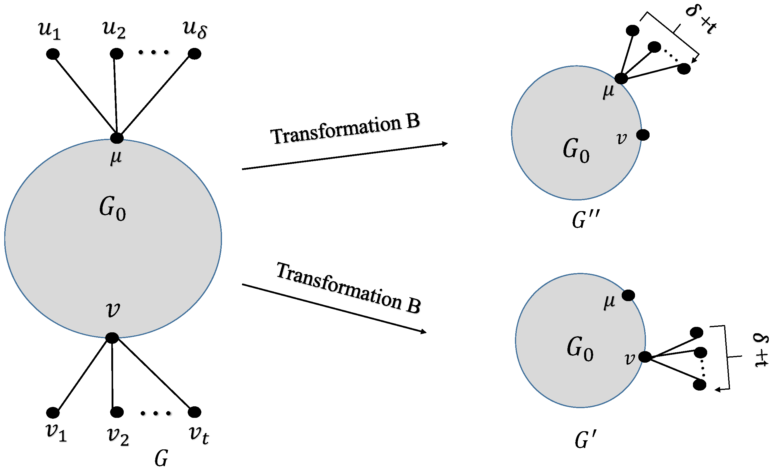
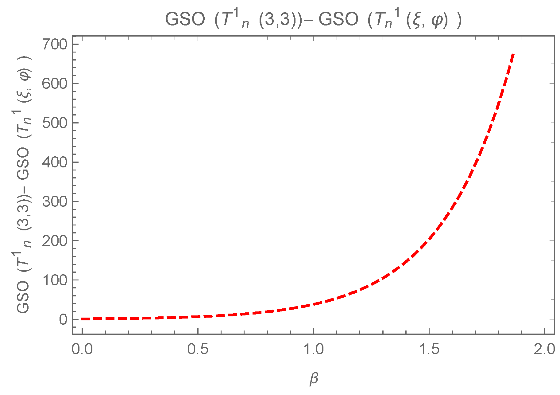
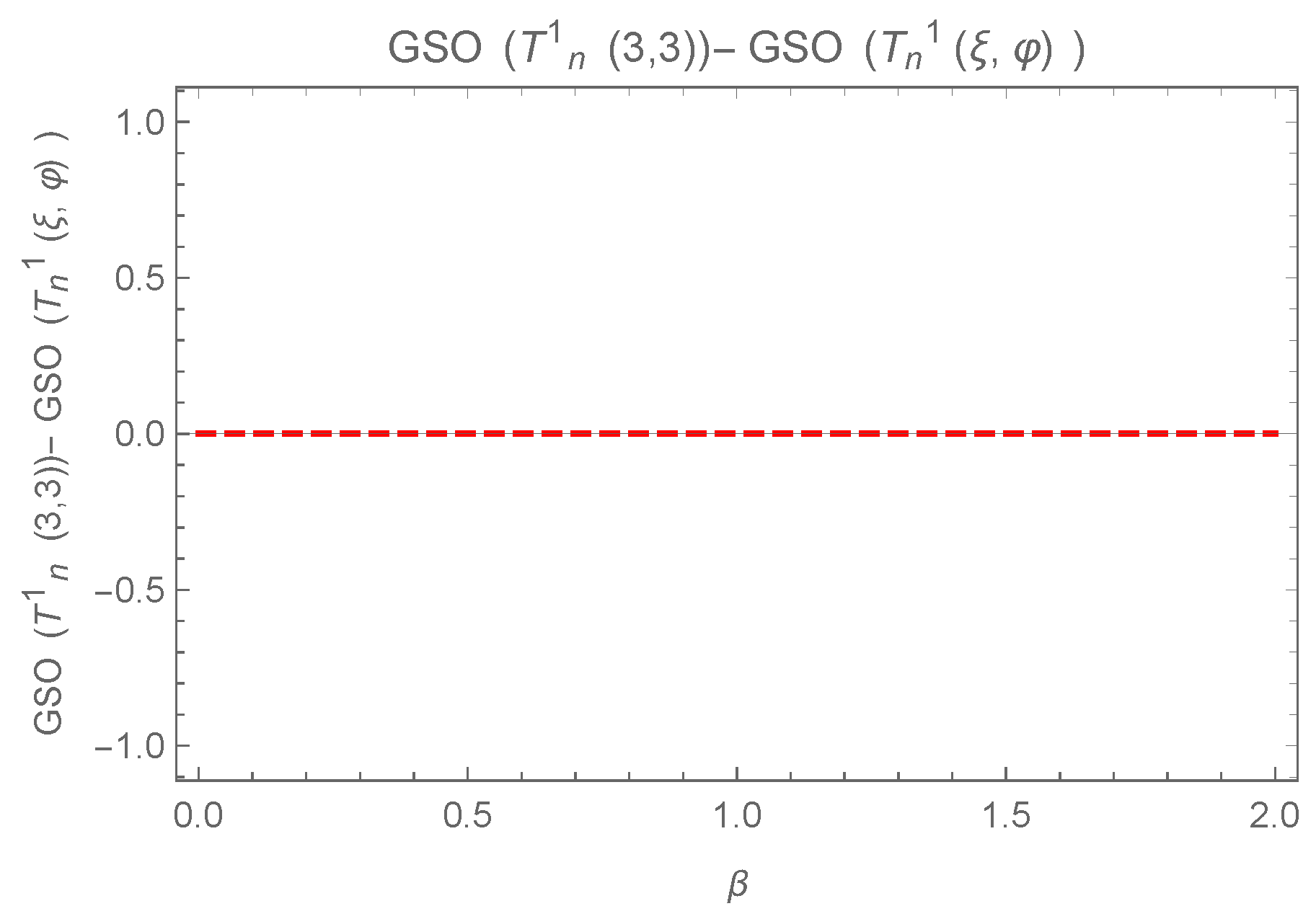
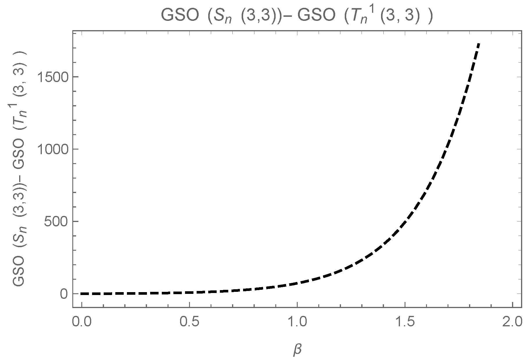
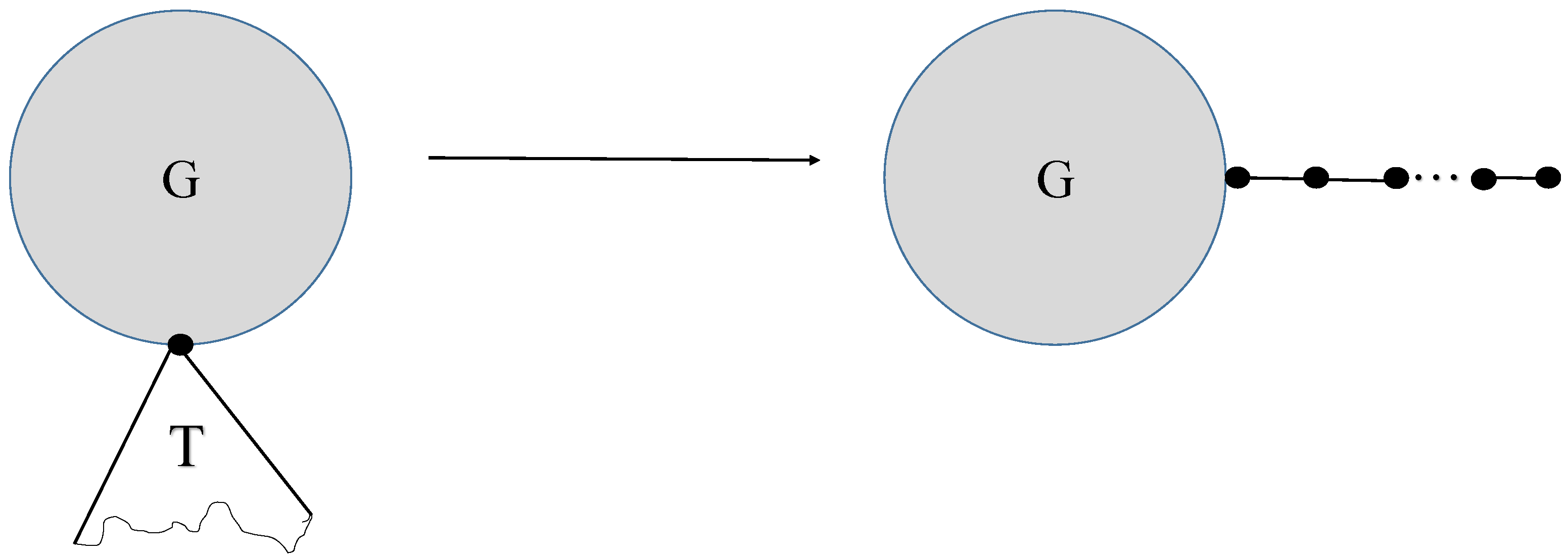
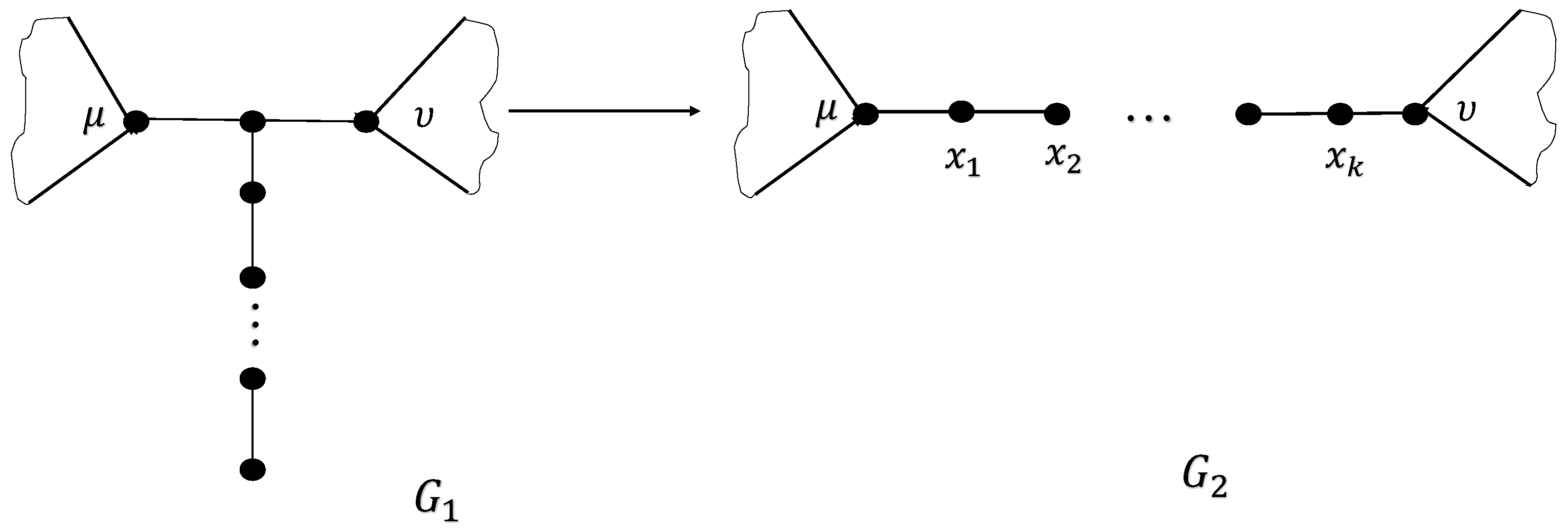
7. Transformation for Decreasing $\mathit{GSO}$

In this section, we investigated the transformation used for decreasing $GSO$.

Transformation C: Consider a simple connected graph G not $P_1$, choose $\mu$ form $V\left(G\right)$. Let $G_1$ is obtained from G by labeling $\mu$ with $v_k$ of the path $v_1{v}_2{v}_3\cdots v_n$, here $1<k<n$. Consider $G_1$, we obtain $G_2$ by deleting $v_{k-1}{v}_k$ and adding $v_n{v}_{k-1}$, we provide Figure 19.

Lemma 7. 

Consider Figure 19, then $GSO\left(G_1\right)>GSO\left(G_2\right)$.

Proof. 

Applying $GSO$, it follows that

$$\begin{array}{cc}& GSO\left(G_1\right)=\sum _{\theta \in N_G\left(\mu \right)}{({(d_G\left(\mu \right)+2)}^2+{\left(d_G\left(\theta \right)\right)}^2)}^{\beta }+{({(d_G\left(\mu \right)+2)}^2+{\left(d_{G_1}\left(v_{k-1}\right)\right)}^2)}^{\beta }\hfill \\ & +{({(2+d_G\left(\mu \right))}^2+{\left(d_{G_1}\left(v_{k+1}\right)\right)}^2)}^{\beta }+{({\left(d_{G_1}\left(v_{n-1}\right)\right)}^2+{\left(d_{G_1}\left(v_n\right)\right)}^2)}^{\beta }.\hfill \end{array}$$

$G_2$ follows that

$$\begin{array}{cc}& GSO\left(G_2\right)=\sum _{\theta \in N_G\left(\mu \right)}{({(1+d_G\left(\mu \right))}^2+{\left(d_G\left(\theta \right)\right)}^2)}^{\beta }+{({(1+d_G\left(\mu \right))}^2+{\left(d_{G_2}\left(v_{k+1}\right)\right)}^2)}^{\beta }\hfill \\ & +{({\left(d_{G_2}\left(v_{n-1}\right)\right)}^2+{\left(d_{G_2}\left(v_n\right)\right)}^2)}^{\beta }+{({\left(d_{G_2}\left(v_n\right)\right)}^2+{\left(d_{G_2}\left(v_{k-1}\right)\right)}^2)}^{\beta }.\hfill \end{array}$$

Here we considered the following:

• Case 1: If $k=2$ and $n=3$.
• In the considered case, the following value is considered:

  $$\begin{array}{cc}& GSO\left(G_1\right)=\sum _{\theta \in N_G\left(\mu \right)}{({(2+d_G\left(\mu \right))}^2+{\left(d_G\left(\theta \right)\right)}^2)}^{\beta }+{({(2+d_G\left(\mu \right))}^2+d_{G_1}{\left(v_1\right)}^2)}^{\beta }\hfill \\ & +{({(2+d_G\left(\mu \right))}^2+d_{G_1}{\left(v_3\right)}^2)}^{\beta },\hfill \\ & =\sum _{\theta \in N_G\left(\mu \right)}{({(2+d_G\left(\mu \right))}^2+{\left(d_G\left(\theta \right)\right)}^2)}^{\beta }+{({(2+d_G\left(\mu \right))}^2+1)}^{\beta }+{({(2+d_G\left(\mu \right))}^2+1)}^{\beta }.\hfill \end{array}$$

  $GSO$ for $G_2$ is given by

  $$\begin{array}{cc}& GSO\left(G_2\right)=\sum _{\theta \in N_G\left(\mu \right)}{({(1+d_G\left(\mu \right))}^2+{\left(d_G\left(\theta \right)\right)}^2)}^{\beta }+{({(1+d_G\left(\mu \right))}^2+d_{G_2}{\left(v_3\right)}^2)}^{\beta }\hfill \\ & +{({\left(d_{G_2}\left({\mu }_3\right)\right)}^2+d_{G_2}{\left(v_1\right)}^2)}^{\beta },\hfill \\ & =\sum _{\theta \in N_G\left(\mu \right)}{({(1+d_G\left(\mu \right))}^2+{\left(d_G\left(\theta \right)\right)}^2)}^{\beta }+{({(1+d_G\left(\mu \right))}^2+4)}^{\beta }+{\left(5\right)}^{\beta }.\hfill \end{array}$$

  $GSO\left(G_1\right)-GSO\left(G_2\right)$ is considered in the following:

  $$\begin{array}{cc}& GSO\left(G_1\right)-GSO\left(G_2\right)=\sum _{\theta \in N_G\left(\mu \right)}{({(2+d_G\left(\mu \right))}^2+{\left(d_G\left(\theta \right)\right)}^2)}^{\beta }+{({(2+d_G\left(\mu \right))}^2+1)}^{\beta }\hfill \\ & +{({(2+d_G\left(\mu \right))}^2+1)}^{\beta }-\sum _{\theta \in N_G\left(\mu \right)}{({(1+d_G\left(\mu \right))}^2+{\left(d_G\left(\theta \right)\right)}^2)}^{\beta }\hfill \\ & -{({(1+d_G\left(\mu \right))}^2+4)}^{\beta }-{\left(5\right)}^{\beta }>0.\hfill \end{array}$$

  Comparing terms of the above last inequality, we obtain $GSO\left(G_1\right)>GSO\left(G_2\right)$.
• Case 2: If $k=2$ and $3<n$.
  The following value is considered:

  $$\begin{array}{cc}& GSO\left(G_1\right)=\sum _{\theta \in N_G\left(\mu \right)}{({(2+d_G\left(\mu \right))}^2+{\left(d_G\left(\theta \right)\right)}^2)}^{\beta }+{({(2+d_G\left(\mu \right))}^2+d_{G_1}{\left(v_1\right)}^2)}^{\beta }\hfill \\ & +{({(2+d_G\left(\mu \right))}^2+d_{G_1}{\left(v_3\right)}^2)}^{\beta }+{({\left(d_{G_1}\left(v_{n-1}\right)\right)}^2+{\left(d_{G_1}\left(v_n\right)\right)}^2)}^{\beta },\hfill \\ & =\sum _{\theta \in N_G\left(\mu \right)}{({(2+d_G\left(\mu \right))}^2+{\left(d_G\left(\theta \right)\right)}^2)}^{\beta }+{({(2+d_G\left(\mu \right))}^2+4)}^{\beta }\hfill \\ & +{({(2+d_G\left(\mu \right))}^2+1)}^{\beta }+{\left(5\right)}^{\beta }.\hfill \end{array}$$

  $GSO$ for $\left(G_2\right)$ is given by

  $$\begin{array}{cc}& GSO\left(G_1\right)=\sum _{\theta \in N_G\left(\mu \right)}{({(1+d_G\left(\mu \right))}^2+{\left(d_G\left(\theta \right)\right)}^2)}^{\beta }+{({(1+d_G\left(\mu \right))}^2+d_{G_1}{\left(v_3\right)}^2)}^{\beta }\hfill \\ & +{({\left(d_{G_2}\left({\mu }_{n-1}\right)\right)}^2+d_{G_2}{\left(v_n\right)}^2)}^{\beta }+{({\left(d_{G_2}\left(v_n\right)\right)}^2+{\left(d_{G_2}\left(v_1\right)\right)}^2)}^{\beta },\hfill \\ & =\sum _{\theta \in N_G\left(\mu \right)}{({(1+d_G\left(\mu \right))}^2+{\left(d_G\left(\theta \right)\right)}^2)}^{\beta }+{({(1+d_G\left(\mu \right))}^2+4)}^{\beta }+{\left(8\right)}^{\beta }+{\left(5\right)}^{\beta }.\hfill \end{array}$$

  The difference of $GSO\left(G_1\right)$ and $GSO\left(G_2\right)$ is given in the following

  $$\begin{array}{cc}& GSO\left(G_1\right)-GSO\left(G_2\right)=\sum _{\theta \in N_G\left(\mu \right)}{({(2+d_G\left(\mu \right))}^2+{\left(d_G\left(\theta \right)\right)}^2)}^{\beta }+{({(2+d_G\left(\mu \right))}^2+4)}^{\beta }\hfill \\ & +{({(2+d_G\left(\mu \right))}^2+1)}^{\beta }+{\left(5\right)}^{\beta }-\sum _{\theta \in N_G\left(\mu \right)}{({(1+d_G\left(\mu \right))}^2+{\left(d_G\left(\theta \right)\right)}^2)}^{\beta }{({(1+d_G\left(\mu \right))}^2+4)}^{\beta }\hfill \\ & -{\left(8\right)}^{\beta }-{\left(5\right)}^{\beta }>0.\hfill \end{array}$$

  Comparing terms of the above last inequality we obtain that $GSO\left(G_1\right)>GSO\left(G_2\right)$.
• Case 3: Consider $2<k$ and $n=k+1$.
  The following value is considered:

  $$\begin{array}{cc}& GSO\left(G_1\right)=\sum _{\theta \in N_G\left(\mu \right)}{({(2+d_G\left(\mu \right))}^2+{\left(d_G\left(\theta \right)\right)}^2)}^{\beta }+{({(2+d_G\left(\mu \right))}^2+d_{G_1}{\left(v_{k+1}\right)}^2)}^{\beta }\hfill \\ & +{({(2+d_G\left(\mu \right))}^2+d_{G_1}{\left(v_{k-1}\right)}^2)}^{\beta },\hfill \\ & =\sum _{\theta \in N_G\left(\mu \right)}{({(2+d_G\left(\mu \right))}^2+{\left(d_G\left(\theta \right)\right)}^2)}^{\beta }+{({(2+d_G\left(\mu \right))}^2+4)}^{\beta }+{({(2+d_G\left(\mu \right))}^2+4)}^{\beta }\hfill \end{array}$$

  $GSO$ for $G_2$ is given in the following:

  $$\begin{array}{cc}& GSO\left(G_2\right)=\sum _{\theta \in N_G\left(\mu \right)}{({(1+d_G\left(\mu \right))}^2+{\left(d_G\left(\theta \right)\right)}^2)}^{\beta }+{({(1+d_G\left(\mu \right))}^2+d_{G_2}{\left(v_{k+1}\right)}^2)}^{\beta }\hfill \\ & +{({\left(d_{G_2}\left(v_{k+1}\right)\right)}^2+d_{G_2}{\left(v_{k-1}\right)}^2)}^{\beta },\hfill \\ & =\sum _{\theta \in N_G\left(\mu \right)}{({(1+d_G\left(\mu \right))}^2+{\left(d_G\left(\theta \right)\right)}^2)}^{\beta }+{({(1+d_G\left(\mu \right))}^2+4)}^{\beta }+{\left(8\right)}^{\beta }.\hfill \end{array}$$

  The difference of $GSO\left(G_1\right)$ and $GSO\left(G_2\right)$ is considered in the following:

  $$\begin{array}{cc}& GSO\left(G_1\right)-GSO\left(G_2\right)=\sum _{\theta \in N_G\left(\mu \right)}{({(2+d_G\left(\mu \right))}^2+{\left(d_G\left(\theta \right)\right)}^2)}^{\beta }+{({(2+d_G\left(\mu \right))}^2+4)}^{\beta }\hfill \\ & +{({(2+d_G\left(\mu \right))}^2+4)}^{\beta }-\sum _{\theta \in N_G\left(\mu \right)}{({(1+d_G\left(\mu \right))}^2+{\left(d_G\left(\theta \right)\right)}^2)}^{\beta }-{({(1+d_G\left(\mu \right))}^2+4)}^{\beta }-{\left(8\right)}^{\beta },\hfill \\ & >0.\hfill \end{array}$$

  Term by term comparison provided that $GSO\left(G_1\right)-GSO\left(G_2\right)>0$, hence $GSO\left(G_1\right)>GSO\left(G_2\right)$.
• Case 4: Consider $2<K$ and $n>k+1$.
  In the desired case, the following value is considered

  $$\begin{array}{cc}& GSO\left(G_1\right)=\sum _{\theta \in N_G\left(\mu \right)}{({(2+d_G\left(\mu \right))}^2+{\left(d_G\left(\theta \right)\right)}^2)}^{\beta }+{({(2+d_G\left(\mu \right))}^2+d_{G_1}{\left(v_{k-1}\right)}^2)}^{\beta }\hfill \\ & +{({(d_G\left(\mu \right)+2)}^2+d_{G_1}{\left(v_{k+1}\right)}^2)}^{\beta }+{({\left(d_{G_1}\left(v_{n-1}\right)\right)}^2+d_{G_1}{\left(v_n\right)}^2)}^{\beta },\hfill \\ & =\sum _{\theta \in N_G\left(\mu \right)}{({(2+d_G\left(\mu \right))}^2+{\left(d_G\left(\theta \right)\right)}^2)}^{\beta }+{({(2+d_G\left(\mu \right))}^2+4)}^{\beta }+{({(2+d_G\left(\mu \right))}^2+4)}^{\beta }+{\left(5\right)}^{\beta }.\hfill \end{array}$$

  $GSO\left(G_2\right)$ is considered in the following:

  $$\begin{array}{cc}& GSO\left(G_2\right)=\sum _{\theta \in N_G\left(\mu \right)}{({(1+d_G\left(\mu \right))}^2+{\left(d_G\left(\theta \right)\right)}^2)}^{\beta }+{({(1+d_G\left(\mu \right))}^2+d_{G_2}{\left(v_{k+1}\right)}^2)}^{\beta }\hfill \\ & +{({\left(d_{G_2}\left(v_{n-1}\right)\right)}^2+d_{G_2}{\left(v_n\right)}^2)}^{\beta }+{({\left(d_{G_2}\left(v_n\right)\right)}^2+d_{G_2}{\left(v_{k-1}\right)}^2)}^{\beta },\hfill \\ & =\sum _{\theta \in N_G\left(\mu \right)}{({(1+d_G\left(\mu \right))}^2+{\left(d_G\left(\theta \right)\right)}^2)}^{\beta }+{({(1+d_G\left(\mu \right))}^2+4)}^{\beta }+{\left(8\right)}^{\beta }+{\left(8\right)}^{\beta }.\hfill \end{array}$$

  The difference of $GSO\left(G_1\right)$ and $GSO\left(G_2\right)$ is considered in the following:

  $$\begin{array}{cc}& GSO\left(G_1\right)=\sum _{\theta \in N_G\left(\mu \right)}{({(2+d_G\left(\mu \right))}^2+{\left(d_G\left(\theta \right)\right)}^2)}^{\beta }+{({(2+d_G\left(\mu \right))}^2+4)}^{\beta }+{({(2+d_G\left(\mu \right))}^2+4)}^{\beta }+{\left(5\right)}^{\beta }\hfill \\ & -\sum _{\theta \in N_G\left(\mu \right)}{({(1+d_G\left(\mu \right))}^2+{\left(d_G\left(\theta \right)\right)}^2)}^{\beta }-{({(1+d_G\left(\mu \right))}^2+4)}^{\beta }-{\left(8\right)}^{\beta }-{\left(8\right)}^{\beta },\hfill \\ & >0.\hfill \end{array}$$

  Term by term comparison provided that ${({(2+d_G\left(\mu \right))}^2+4)}^{\beta }+{\left(5\right)}^{\beta }-{\left(8\right)}^{\beta }-{\left(8\right)}^{\beta }>0$. Hence it follows that $GSO\left(G_1\right)-GSO\left(G_2\right)>0$.

□

Remark 3. 

Using Transformation  C  repeatedly, we transform any tree to a path and $GSO$ decreases, Figure 20 is given for this.

Transformation D: Consider a graph G, let $\mu$ and v are in G. We obtain $G_1$ by marking $\mu$ with $u_0$ and v with $v_0$ of the considered paths $u_0{u}_1\cdots u_{\delta -1}{u}_{\delta }$ and $v_0{v}_1\cdots v_{t-1}{v}_t$, respectively. Let $G_2$ be the graph which is obtained from $G_1$ by removing $u_0{u}_1$ and add $v_t{u}_1$ as in Figure 21.

Lemma 8. 

Consider $G_1$ and $G_2$ as in Figure 21, with $1<d_G\left(v\right)\le d_G\left(\mu \right)$, $1\le \delta$ and $0\le t$, then

(i) 

For $0<t$, we have $GSO\left(G_2\right)<GSO\left(G_1\right)$;

(ii) 

For $t=0$ and ${\sum }_{y\in \{N_G\left(v\right)-\left\{\mu \right\}\}}{d}_G\left(y\right)<{\sum }_{\theta \in \{N_G\left(\mu \right)-\left\{v\right\}\}}{d}_G\left(\theta \right)$, we have $GSO\left(G_2\right)<GSO\left(G_1\right)$.

Proof. 

(i) As $1<d_G\left(\mu \right)$ and $0<t$, then we consider the following cases;

• Case 1. For $t=1$ and $\delta =1$.
  In the considered case, for $GSO\left(G_1\right)$ we have the following:

  $$\begin{array}{cc}& GSO\left(G_1\right)=\sum _{\theta \in N_G\left(\mu \right)}{({(d_G\left(\mu \right)+1)}^2+{\left(d_G\left(\theta \right)\right)}^2)}^{\beta }+{({(d_G\left(\mu \right)+1)}^2+d_{G_1}{\left({\mu }_1\right)}^2)}^{\beta }\hfill \\ & +{({(d_G\left(v\right)+1)}^2+d_{G_1}{\left(v_1\right)}^2)}^{\beta },\hfill \\ & =\sum _{\theta \in N_G\left(\mu \right)}{({(d_G\left(\mu \right)+1)}^2+{\left(d_G\left(\theta \right)\right)}^2)}^{\beta }+{({(d_G\left(\mu \right)+1)}^2+1)}^{\beta }+{({(d_G\left(v\right)+1)}^2+1)}^{\beta }.\hfill \end{array}$$

  $GSO\left(G_2\right)$ is considered in the following:

  $$\begin{array}{cc}& GSO\left(G_2\right)=\sum _{\theta \in N_G\left(\mu \right)}{({\left(d_G\left(\mu \right)\right)}^2+{\left(d_G\left(\theta \right)\right)}^2)}^{\beta }+{({(d_G\left(v\right)+1)}^2+d_{G_2}{\left(v_1\right)}^2)}^{\beta }\hfill \\ & +{({\left(d_{G_2}\left(v_1\right)\right)}^2+d_{G_2}{\left({\mu }_1\right)}^2)}^{\beta },\hfill \\ & =\sum _{\theta \in N_G\left(\mu \right)}{({\left(d_G\left(\mu \right)\right)}^2+{\left(d_G\left(\theta \right)\right)}^2)}^{\beta }+{({(d_G\left(v\right)+1)}^2+4)}^{\beta }+{\left(5\right)}^{\beta }.\hfill \end{array}$$

  The difference of $GSO\left(G_1\right)$ and $GSO\left(G_2\right)$ is considered in the following

  $$\begin{array}{cc}& GSO\left(G_1\right)-GSO\left(G_2\right)=\sum _{\theta \in N_G\left(\mu \right)}{({(d_G\left(\mu \right)+1)}^2+{\left(d_G\left(\theta \right)\right)}^2)}^{\beta }+{({(d_G\left(\mu \right)+1)}^2+1)}^{\beta }\hfill \\ & +{({(d_G\left(v\right)+1)}^2+1)}^{\beta }-\sum _{\theta \in N_G\left(\mu \right)}{({\left(d_G\left(\mu \right)\right)}^2+{\left(d_G\left(\theta \right)\right)}^2)}^{\beta }-{({(d_G\left(v\right)+1)}^2+4)}^{\beta }-{\left(5\right)}^{\beta },\hfill \\ & >0,\because d_G\left(\mu \right)\ge d_G\left(v\right).\hfill \end{array}$$

  Hence $GSO\left(G_1\right)>GSO\left(G_2\right)$.
• Case 2. If $t>1$ and $\delta =1$.
  In the considered case, we have $GSO\left(G_1\right)$ in the following

  $$\begin{array}{cc}& GSO\left(G_1\right)=\sum _{\theta \in N_G\left(\mu \right)}{({(d_G\left(\mu \right)+1)}^2+{\left(d_G\left(\theta \right)\right)}^2)}^{\beta }+{({(d_G\left(\mu \right)+1)}^2+d_{G_1}{\left({\mu }_1\right)}^2)}^{\beta }\hfill \\ & +{({\left(d_{G_1}\left(v_{t-1}\right)\right)}^2+d_{G_1}{\left(v_t\right)}^2)}^{\beta },\hfill \\ & =\sum _{\theta \in N_G\left(\mu \right)}{({(d_G\left(\mu \right)+1)}^2+{\left(d_G\left(\theta \right)\right)}^2)}^{\beta }+{({(d_G\left(\mu \right)+1)}^2+1)}^{\beta }+{\left(5\right)}^{\beta }\hfill \end{array}$$

  $GSO\left(G_2\right)$ is considered in the following:

  $$\begin{array}{cc}& GSO\left(G_2\right)=\sum _{\theta \in N_G\left(\mu \right)}{({\left(d_G\left(\mu \right)\right)}^2+{\left(d_G\left(\theta \right)\right)}^2)}^{\beta }+{({\left(d_{G_2}\left(v_{t-1}\right)\right)}^2+d_{G_2}{\left(v_t\right)}^2)}^{\beta }\hfill \\ & +{({\left(d_{G_2}\left(v_t\right)\right)}^2+d_{G_2}{\left({\mu }_1\right)}^2)}^{\beta },\hfill \\ & =\sum _{\theta \in N_G\left(\mu \right)}{({\left(d_G\left(\mu \right)\right)}^2+{\left(d_G\left(\theta \right)\right)}^2)}^{\beta }+{\left(8\right)}^{\beta }+{\left(5\right)}^{\beta }.\hfill \end{array}$$

  $GSO\left(G_1\right)-GSO\left(G_2\right)$ is considered in the following:

  $$\begin{array}{cc}& GSO\left(G_1\right)-GSO\left(G_2\right)=\sum _{\theta \in N_G\left(\mu \right)}{({(d_G\left(\mu \right)+1)}^2+{\left(d_G\left(\theta \right)\right)}^2)}^{\beta }+{({(d_G\left(\mu \right)+1)}^2+1)}^{\beta }+{\left(5\right)}^{\beta }\hfill \\ & -\sum _{\theta \in N_G\left(\mu \right)}{({\left(d_G\left(\mu \right)\right)}^2+{\left(d_G\left(\theta \right)\right)}^2)}^{\beta }-{\left(8\right)}^{\beta }-{\left(5\right)}^{\beta }>0.\hfill \end{array}$$

  Hence $GSO\left(G_1\right)>GSO\left(G_2\right)$.
• Case 3. If $1<\delta$ and $t=1$.
  In the considered case, $GSO\left(G_1\right)$ is given by

  $$\begin{array}{cc}& GSO\left(G_1\right)=\sum _{\theta \in N_G\left(\mu \right)}{({(d_G\left(\mu \right)+1)}^2+{\left(d_G\left(\theta \right)\right)}^2)}^{\beta }+{({(d_G\left(\mu \right)+1)}^2+d_{G_1}{\left({\mu }_1\right)}^2)}^{\beta }\hfill \\ & +{({(d_G\left(v\right)+1)}^2+d_{G_1}{\left(v_1\right)}^2)}^{\beta },\hfill \\ & =\sum _{\theta \in N_G\left(\mu \right)}{({(d_G\left(\mu \right)+1)}^2+{\left(d_G\left(\theta \right)\right)}^2)}^{\beta }+{({(d_G\left(\mu \right)+1)}^2+4)}^{\beta }+{({(d_G\left(v\right)+1)}^2+1)}^{\beta }.\hfill \\ \end{array}$$

  The value of $GSO\left(G_2\right)$ is considered below

  $$\begin{array}{cc}& GSO\left(G_2\right)=\sum _{\theta \in N_G\left(\mu \right)}{({\left(d_G\left(\mu \right)\right)}^2+{\left(d_G\left(\theta \right)\right)}^2)}^{\beta }+{({(d_G\left(v\right)+1)}^2+d_{G_2}{\left(v_1\right)}^2)}^{\beta }\hfill \\ & +{({\left(d_{G_2}\left(v_1\right)\right)}^2+d_{G_2}{\left({\mu }_1\right)}^2)}^{\beta },\hfill \\ & =\sum _{\theta \in N_G\left(\mu \right)}{({\left(d_G\left(\mu \right)\right)}^2+{\left(d_G\left(\theta \right)\right)}^2)}^{\beta }+{({(d_G\left(v\right)+1)}^2+4)}^{\beta }+{\left(8\right)}^{\beta }.\hfill \end{array}$$

  $GSO\left(G_1\right)-GSO\left(G_1\right)$ is considered in the following:

  $$\begin{array}{cc}& GSO\left(G_1\right)-GSO\left(G_2\right)=\sum _{\theta \in N_G\left(\mu \right)}{({(d_G\left(\mu \right)+1)}^2+{\left(d_G\left(\theta \right)\right)}^2)}^{\beta }+{({(d_G\left(\mu \right)+1)}^2+4)}^{\beta }\hfill \\ & +{({(d_G\left(v\right)+1)}^2+1)}^{\beta }-\sum _{\theta \in N_G\left(\mu \right)}{({\left(d_G\left(\mu \right)\right)}^2+{\left(d_G\left(\theta \right)\right)}^2)}^{\beta }\hfill \\ & -{({(d_G\left(v\right)+1)}^2+4)}^{\beta }-{\left(8\right)}^{\beta }>0.\hfill \\ \end{array}$$

  Here we have $GSO\left(G_1\right)>GSO\left(G_2\right)$.
• Case 4. If $1<\delta$ and $t>1$.
  In the considered case, $GSO\left(G_1\right)$ is given by

  $$\begin{array}{cc}& GSO\left(G_1\right)=\sum _{\theta \in N_G\left(\mu \right)}{({(d_G\left(\mu \right)+1)}^2+{\left(d_G\left(\theta \right)\right)}^2)}^{\beta }+{({(d_G\left(\mu \right)+1)}^2+d_{G_1}{\left({\mu }_1\right)}^2)}^{\beta }\hfill \\ & +{({\left(d_{G_1}\left(v_{t-1}\right)\right)}^2+d_{G_1}{\left(v_t\right)}^2)}^{\beta },\hfill \\ & =\sum _{\theta \in N_G\left(\mu \right)}{({(d_G\left(\mu \right)+1)}^2+{\left(d_G\left(\theta \right)\right)}^2)}^{\beta }+{({(d_G\left(\mu \right)+1)}^2+4)}^{\beta }+{\left(5\right)}^{\beta }.\hfill \end{array}$$

  $GSO\left(G_2\right)$ is considered in the following:

  $$\begin{array}{cc}& GSO\left(G_2\right)=\sum _{\theta \in N_G\left(\mu \right)}{({\left(d_G\left(\mu \right)\right)}^2+{\left(d_G\left(\theta \right)\right)}^2)}^{\beta }+{({\left(d_{G_2}\left(v_{t-1}\right)\right)}^2+d_{G_2}{\left(v_t\right)}^2)}^{\beta }\hfill \\ & +{({\left(d_{G_2}\left(v_t\right)\right)}^2+d_{G_2}{\left({\mu }_1\right)}^2)}^{\beta },\hfill \\ & =\sum _{\theta \in N_G\left(\mu \right)}{({\left(d_G\left(\mu \right)\right)}^2+{\left(d_G\left(\theta \right)\right)}^2)}^{\beta }+{\left(8\right)}^{\beta }+{\left(5\right)}^{\beta }.\hfill \end{array}$$

  The following difference is considered

  $$\begin{array}{cc}& GSO\left(G_1\right)=\sum _{\theta \in N_G\left(\mu \right)}{({(d_G\left(\mu \right)+1)}^2+{\left(d_G\left(\theta \right)\right)}^2)}^{\beta }+{({(d_G\left(\mu \right)+1)}^2+4)}^{\beta }+{\left(5\right)}^{\beta }\hfill \\ & -\sum _{\theta \in N_G\left(\mu \right)}{({\left(d_G\left(\mu \right)\right)}^2+{\left(d_G\left(\theta \right)\right)}^2)}^{\beta }+{\left(8\right)}^{\beta }+{\left(5\right)}^{\beta }>0.\hfill \end{array}$$

  Hence $GSO\left(G_1\right)-GSO\left(G_2\right)$ and $GSO\left(G_1\right)>GSO\left(G_2\right)$.
  (ii). For $t=0$ and ${\sum }_{y\in N_G\left(v\right)-\left\{\mu \right\}}{d}_G\left(y\right)<{\sum }_{\theta \in N_G\left(\mu \right)-\left\{v\right\}}{d}_G\left(\theta \right)$, if v and $\mu$ are adjacent then the following is considered:

  $$\begin{array}{cc}& GSO\left(G_1\right)=\sum _{\theta \in N_G\left(\mu \right)}{({(d_G\left(\mu \right)+1)}^2+{\left(d_G\left(\theta \right)\right)}^2)}^{\beta }+{({(d_G\left(\mu \right)+1)}^2+d_{G_1}{\left({\mu }_1\right)}^2)}^{\beta }\hfill \\ & +\sum _{y\in N_G\left(v\right)}{({\left(d_G\left(v\right)\right)}^2+d_G{\left(y\right)}^2)}^{\beta }.\hfill \end{array}$$

  $GSO\left(G_2\right)$ is considered below.

  $$\begin{array}{cc}& GSO\left(G_2\right)=\sum _{\theta \in N_G\left(\mu \right)}{({\left(d_G\left(\mu \right)\right)}^2+{\left(d_G\left(\theta \right)\right)}^2)}^{\beta }+{({(d_G\left(v\right)+1)}^2+d_{G_2}{\left({\mu }_1\right)}^2)}^{\beta }\hfill \\ & +\sum _{y\in N_G\left(v\right)}{({(d_G\left(v\right)+1)}^2+d_G{\left(y\right)}^2)}^{\beta }.\hfill \end{array}$$

  $GSO\left(G_1\right)-GSO\left(G_2\right)$ is considered in the following:

  $$\begin{array}{cc}& GSO\left(G_1\right)-GSO\left(G_2\right)=\sum _{\theta \in N_G\left(\mu \right)}{({(d_G\left(\mu \right)+1)}^2+{\left(d_G\left(\theta \right)\right)}^2)}^{\beta }+{({(d_G\left(\mu \right)+1)}^2+d_{G_1}{\left({\mu }_1\right)}^2)}^{\beta }\hfill \\ & +\sum _{y\in N_G\left(v\right)}{({\left(d_G\left(v\right)\right)}^2+d_G{\left(y\right)}^2)}^{\beta }-\sum _{\theta \in N_G\left(\mu \right)}{({\left(d_G\left(\mu \right)\right)}^2+{\left(d_G\left(\theta \right)\right)}^2)}^{\beta }.\hfill \\ & -{({(d_G\left(v\right)+1)}^2+d_{G_2}{\left({\mu }_1\right)}^2)}^{\beta }-\sum _{y\in N_G\left(v\right)}{({(d_G\left(v\right)+1)}^2+d_G{\left(y\right)}^2)}^{\beta },\hfill \\ & >0.\because d_{G_1}\left({\mu }_1\right)=d_{G_2}\left({\mu }_1\right)\hfill \end{array}$$

  The above inequality provided that $GSO\left(G_1\right)>GSO\left(G_2\right)$.
  If v and $\mu$ are adjacent, then

  $$\begin{array}{cc}& GSO\left(G_1\right)=\sum _{\theta \in N_G\left(\mu \right)-\left\{v\right\}}{({(d_G\left(\mu \right)+1)}^2+{\left(d_G\left(\theta \right)\right)}^2)}^{\beta }+{({(d_G\left(\mu \right)+1)}^2+d_{G_1}{\left({\mu }_1\right)}^2)}^{\beta }\hfill \\ & +\sum _{y\in N_G\left(v\right)-\left\{\mu \right\}}{({\left(d_G\left(v\right)\right)}^2+d_G{\left(y\right)}^2)}^{\beta }+{({(d_G\left(\mu \right)+1)}^2+{\left(d_G\left(v\right)\right)}^2)}^{\beta }.\hfill \end{array}$$

  For $GSO\left(G_2\right)$, it follows that

  $$\begin{array}{cc}& GSO\left(G_2\right)=\sum _{\theta \in N_G\left(\mu \right)-\left\{v\right\}}{({\left(d_G\left(\mu \right)\right)}^2+{\left(d_G\left(\theta \right)\right)}^2)}^{\beta }+{({(d_G\left(v\right)+1)}^2+d_{G_2}{\left({\mu }_1\right)}^2)}^{\beta }\hfill \\ & +\sum _{y\in N_G\left(v\right)-\left\{\mu \right\}}{({(d_G\left(v\right)+1)}^2+d_G{\left(y\right)}^2)}^{\beta }+{({\left(d_G\left(\mu \right)\right)}^2+{(d_G\left(v\right)+1)}^2)}^{\beta }.\hfill \end{array}$$

  $GSO\left(G_1\right)-GSO\left(G_2\right)$ is considered in the following:

  $$\begin{array}{cc}& GSO\left(G_1\right)-GSO\left(G_2\right)=\hfill \\ & \sum _{\theta \in N_G\left(\mu \right)-\left\{v\right\}}{({(d_G\left(\mu \right)+1)}^2+{\left(d_G\left(\theta \right)\right)}^2)}^{\beta }+{({(d_G\left(\mu \right)+1)}^2+d_{G_1}{\left({\mu }_1\right)}^2)}^{\beta }\hfill \\ & +\sum _{y\in N_G\left(v\right)-\left\{\mu \right\}}{({\left(d_G\left(v\right)\right)}^2+d_G{\left(y\right)}^2)}^{\beta }+{({(d_G\left(\mu \right)+1)}^2+{\left(d_G\left(v\right)\right)}^2)}^{\beta }\hfill \\ & -\sum _{\theta \in N_G\left(\mu \right)-\left\{v\right\}}{({\left(d_G\left(\mu \right)\right)}^2+{\left(d_G\left(\theta \right)\right)}^2)}^{\beta }-{({(d_G\left(v\right)+1)}^2+d_{G_2}{\left({\mu }_1\right)}^2)}^{\beta }\hfill \\ & -\sum _{y\in N_G\left(v\right)-\left\{\mu \right\}}{({(d_G\left(v\right)+1)}^2+d_G{\left(y\right)}^2)}^{\beta }-{({\left(d_G\left(\mu \right)\right)}^2+{(d_G\left(v\right)+1)}^2)}^{\beta },\hfill \\ & >0.\because d_{G_1}\left({\mu }_1\right)=d_{G_2}\left({\mu }_1\right)\hfill \end{array}$$

  Hence $GSO\left(G_1\right)-GSO\left(G_2\right)$ and $GSO\left(G_1\right)>GSO\left(G_2\right)$.

□

Remark 4. 

Apply Transformation C and Transformation D repeatedly. We change every tree to a path and every unicyclic graph to a unicyclic graph in which the path is attached to the cycle. Any bicyclic graph can be transformed to a bicyclic graph where the path is attached to the graph in Figure 22 (Lemma 8(i)). We transform any bicyclic graph to a new bicyclic graph where the path is attached to the vertex of degree 2 (Lemma 8(ii)), general Sombor index minimizes.

Lemma 9. 

Consider a graph $G_1$ given in the Figure 23, let us consider a path $x_k,x_{k-1},x_{k-2},\cdots ,x_3,$$x_2,x_1$, where $1<k$ attached to vertex $x_1$. We obtain $G_2$ from $G_1$ by removing $v{x}_1$ and attach $v{x}_k$, then $GSO\left(G_1\right)>GSO\left(G_2\right)$.

Proof. 

Here, $d\left(x_k\right)$ and $d\left(x_1\right)$ are not same. If $k=2$, then the following is considered

$$\begin{array}{cc}& GSO\left(G_1\right)={(d{\left(\mu \right)}^2+d_{G_1}{\left(x_1\right)}^2)}^{\beta }+{(d_{G_1}{\left(x_1\right)}^2+d_{G_1}{\left(x_2\right)}^2)}^{\beta }+{(d_{G1}{\left(x_1\right)}^2+d{\left(v\right)}^2)}^{\beta },\hfill \\ & ={(d{\left(\mu \right)}^2+9)}^{\beta }+{\left(10\right)}^{\beta }+{(9+d{\left(v\right)}^2)}^{\beta }.\hfill \end{array}$$

$GSO\left(G_2\right)$ is considered below.

$$\begin{array}{cc}& GSO\left(G_2\right)={(d{\left(\mu \right)}^2+d_{G_2}{\left(x_1\right)}^2)}^{\beta }+{(d_{G_2}{\left(x_1\right)}^2+d_{G_2}{\left(x_2\right)}^2)}^{\beta }+{(d_{G2}{\left(x_2\right)}^2+d{\left(v\right)}^2)}^{\beta },\hfill \\ & ={(d{\left(\mu \right)}^2+4)}^{\beta }+{\left(8\right)}^{\beta }+{(4+d{\left(v\right)}^2)}^{\beta }.\hfill \end{array}$$

Considering $GSO\left(G_1\right)-GSO\left(G_2\right)$ below

$$\begin{array}{cc}& GSO\left(G_1\right)-GSO\left(G_2\right)={(d{\left(\mu \right)}^2+27)}^{\beta }+{\left(28\right)}^{\beta }+{(27+d{\left(v\right)}^2)}^{\beta }\hfill \\ & -{(d{\left(\mu \right)}^2+4)}^{\beta }-{\left(8\right)}^{\beta }-{(4+d{\left(v\right)}^2)}^{\beta },\hfill \\ & >0.\hfill \end{array}$$

Let $2<k$, then for $GSO\left(G_1\right)$ the following is considered

$$\begin{array}{cc}& GSO\left(G_1\right)={(d{\left(\mu \right)}^2+d_{G_1}{\left(x_1\right)}^2)}^{\beta }+{(d_{G_1}{\left(x_1\right)}^2+d_{G_1}{\left(x_2\right)}^2)}^{\beta }\hfill \\ & +{(d_{G1}{\left(x_1\right)}^2+d{\left(v\right)}^2)}^{\beta }+{(d_{G_1}{\left(x_{k-1}\right)}^2+d_{G_1}{\left(x_k\right)}^2)}^{\beta },\hfill \\ & ={(d{\left(\mu \right)}^2+9)}^{\beta }+{\left(13\right)}^{\beta }+{(9+d{\left(v\right)}^2)}^{\beta }+{\left(5\right)}^{\beta }.\hfill \end{array}$$

$GSO\left(G_1\right)$ is considered in the following:

$$\begin{array}{cc}& GSO\left(G_2\right)={(d{\left(\mu \right)}^2+d_{G_2}{\left(x_1\right)}^2)}^{\beta }+{(d_{G_2}{\left(x_1\right)}^2+d_{G_2}{\left(x_2\right)}^2)}^{\beta }\hfill \\ & +{(d_{G_2}{\left(x_k\right)}^2+d{\left(v\right)}^2)}^{\beta }+{(d_{G2}{\left(x_{k-1}\right)}^2+d_{G2}{\left(x_k\right)}^2)}^{\beta },\hfill \\ & ={(d{\left(\mu \right)}^2+4)}^{\beta }+{\left(8\right)}^{\beta }+{(4+d{\left(v\right)}^2)}^{\beta }+{\left(8\right)}^{\beta }.\hfill \end{array}$$

$GSO\left(G_1\right)-GSO\left(G_2\right)$ is in the following:

$$\begin{array}{cc}& GSO\left(G_1\right)-GSO\left(G_{12}\right)={(d{\left(\mu \right)}^2+9)}^{\beta }+{(9+d{\left(v\right)}^2)}^{\beta }-{(d{\left(\mu \right)}^2+4)}^{\beta }-{(4+d{\left(v\right)}^2)}^{\beta }\hfill \\ & +{\left(13\right)}^{\beta }+{\left(5\right)}^{\beta }-2{\left(8\right)}^{\beta }>0.\hfill \end{array}$$

We obtain that $GSO\left(G_1\right)-GSO\left(G_2\right)>0$ and $GSO\left(G_1\right)>GSO\left(G_2\right)$. □

8. The Smallest $\mathit{GSO}$ in Trees, Unicyclic, and Bicyclic Graphs

In this section, the general Sombor index is investigated in trees, unicyclic, and bicyclic graphs for minimum values. From Lemma 7, it follows that

Theorem 8. 

Consider a tree T of order n, if $T\ne P_n$ then $GSO\left(T_n\right)>GSO\left(P_n\right)$.

Consider $U_n^k$ be a unicyclic graph obtained by attaching a path of length $n-k$ to $C_k$. Using Lemmas 7 and 8, it follows that

Theorem 9. 

Consider a unicyclic graph G with order n and girth k. If $G\ne U_n^k$, then $GSO\left(U_n^k\right)<GSO\left(G\right)$.

By means of Lemma 9, the following is obtained:

Theorem 10. 

$C_n$ is the unique graph with smallest $GSO$.

Let $J_1$, $J_2$, and $J_3$ be as shown in Figure 22. From Lemmas 7 and 9, the bicyclic graph with the smallest general Sombor index is given by

$$\begin{array}{cc}& GSO\left(J_1\right)=(n-3)8^{\beta }+4{\left(20\right)}^{\beta }.\hfill \end{array}$$

$$\begin{array}{cc}& GSO\left(J_2\right)=GSO\left(J_3\right)=(n-4)8^{\beta }+4{\left(13\right)}^{\beta }+{\left(18\right)}^{\beta },\hfill \end{array}$$

if v and $\mu$ are directly connected by an edge

$$\begin{array}{cc}& GSO\left(J_2\right)=GSO\left(J_3\right)=(n-5)8^{\beta }+6{\left(13\right)}^{\beta },\hfill \end{array}$$

if v and $\mu$ are not connected directly by an edge. We have the following differences:

$$GSO\left(J_1\right)-GSO\left(J_2\right)=8^{\beta }+4{\left(20\right)}^{\beta }-4{\left(13\right)}^{\beta }-{\left(18\right)}^{\beta }>0.$$

Figure 24 is provided for the difference.

$$GSO\left(J_1\right)-GSO\left(J_3\right)=2\left(8^{\beta }\right)+4{\left(20\right)}^{\beta }-6{\left(13\right)}^{\beta }>0.$$

$$GSO\left(J_2\right)-GSO\left(J_3\right)=8^{\beta }+4{\left(13\right)}^{\beta }+{\left(18\right)}^{\beta }-6{\left(13\right)}^{\beta }>0.$$

For the last inequality, we provide Figure 25.

Hence, it follows that

Theorem 11. 

Let G be the family of bicyclic graphs of order n, then the largest $GSO$ is for the graph $J_1$.

Theorem 12. 

Let G be the family of bicyclic graphs of order n, then the smallest $GSO$ is for $J_3$ where the vertices of degree 3 are not adjacent, that is $GSO\left(J_1\right)>GSO\left(J_2\right)>GSO\left(J_3\right)$.

9. Conclusions

In this work, the generalized Sombor index is investigated for optimal values in graphs. Various transformations are used for obtaining graphs with optimal values in the family of bicyclic graphs, trees, and unicyclic graphs. The considered transformations are simple and very easy to understand. The effectiveness of these transformations has been demonstrated through rigorous theorems and visualized using comparative plots. Our results contribute to the deeper understanding of the behavior of the generalized Sombor index and offer useful tools for future studies in topological indices.

References

- Balakrishnan, V.K. Schaum’s Outline of Theory and Problems of Graph Theory; McGraw-Hill: New York, NY, USA, 1997. [Google Scholar]
- Khan, M.Y.; Ali, G.; Popa, I.L. Optimization of General Power-Sum Connectivity Index in Uni-Cyclic Graphs, Bi-Cyclic Graphs and Trees by Means of Operations. Axioms 2024, 13, 840. [Google Scholar] [CrossRef]
- Khan, M.Y.; Ali, G.; Popa, I.L. Optimization in Symmetric Trees, Unicyclic Graphs, and Bicyclic Graphs with Help of Mappings Using Second Form of Generalized Power-Sum Connectivity Index. Symmetry 2025, 17, 122. [Google Scholar] [CrossRef]
- Diudea, M.V.; Gutman, I.; Jantschi, L. Molecular Topology; Nova Science Publishers: Huntington, NY, USA, 2001. [Google Scholar]
- Mahasinghe, A.C.; Erandi, K.K.W.H.; Perera, S.S.N. Optimizing Wiener and Randić Indices of Graphs. Adv. Oper. Res. 2020, 2020, 3139867. [Google Scholar] [CrossRef]
- Gutman, I.; Mohar, B. The quasi-Wiener and the Kirchhoff indices coincide. J. Chem. Inf. Comput. Sci. 1996, 36, 982–985. [Google Scholar] [CrossRef]
- Otte, E.; Rousseau, R. Social network analysis: A powerful strategy, also for the information sciences. J. Inf. Sci. 2002, 28, 441–453. [Google Scholar] [CrossRef]
- Imran, M.; Hayat, S.; Mailk, M.Y.H. On topological indices of certain interconnection networks. Appl. Math. Comput. 2014, 244, 936–951. [Google Scholar] [CrossRef]
- Kier, L.B. Indexes of molecular shape from chemical graphs. Med. Res. Rev. 1987, 7, 417–440. [Google Scholar] [CrossRef] [PubMed]
- Camarda, K.V.; Maranas, C.D. Optimization in polymer design using connectivity indices. Ind. Eng. Chem. Res. 1999, 38, 1884–1892. [Google Scholar] [CrossRef]
- Matamala, A.R.; Estrada, E. Generalised topological indices: Optimisation methodology and physico-chemical interpretation. Chem. Phys. Lett. 2005, 410, 343–347. [Google Scholar] [CrossRef]
- Preuß, M.; Dehmer, M.; Pickl, S.; Holzinger, A. On terrain coverage optimization by using a network approach for universal graph-based data mining and knowledge discovery. In Brain Informatics and Health, Proceedings of the International Conference, BIH 2014, Warsaw, Poland, 11–14 August 2014; Proceedings; Springer International Publishing: Berlin/Heidelberg, Germany, 2014; pp. 564–573. [Google Scholar]
- Che, Z.; Chen, Z. Lower and upper bounds of the forgotten topological index. MATCH Commun. Math. Comput. Chem. 2016, 76, 635–648. [Google Scholar]
- Monsalve, J.; Rada, J. Sharp upper and lower bounds of VDB topological indices of digraphs. Symmetry 2021, 13, 1903. [Google Scholar] [CrossRef]
- Martínez-Pérez, Á.; Rodríguez, J.M. New bounds for topological indices on trees through generalized methods. Symmetry 2020, 12, 1097. [Google Scholar] [CrossRef]
- Martínez-Pérez, Á.; Rodríguez, J. M Upper and lower bounds for topological indices on unicyclic graphs. Topol. Its Appl. 2023, 339, 108591. [Google Scholar] [CrossRef]
- Wei, C.C.; Salman, M.; Ali, U.; Rehman, M.U.; Khan, M.A.A.; Chaudary, M.H.; Ahmad, F. Some topological invariants of graphs associated with the group of symmetries. J. Chem. 2020, 2020, 6289518. [Google Scholar] [CrossRef]
- Chu, P.; Li, Y.; He, Z.; Li, E.; Ozgun, O.; Venbosch, G.A.; Zheng, X. A group theory based topology optimization scheme for the design of inhomogeneous waveguides with dihedral group symmetries. Eng. Anal. Bound. Elem. 2024, 166, 105845. [Google Scholar] [CrossRef]
- Öztürk Sözen, E.; Alsuraiheed, T.; Abdioğlu, C.; Ali, S. Computing topological descriptors of prime ideal sum graphs of commutative rings. Symmetry 2023, 15, 2133. [Google Scholar] [CrossRef]
- Balasubramanian, K. Topological indices, graph spectra, entropies, Laplacians, and matching polynomials of n-dimensional hypercubes. Symmetry 2023, 15, 557. [Google Scholar] [CrossRef]
- Kosaka, I.; Swan, C.C. A symmetry reduction method for continuum structural topology optimization. Comput. Struct. 1999, 70, 47–61. [Google Scholar] [CrossRef]
Disclaimer/Publisher’s Note: The statements, opinions and data contained in all publications are solely those of the individual author(s) and contributor(s) and not of MDPI and/or the editor(s). MDPI and/or the editor(s) disclaim responsibility for any injury to people or property resulting from any ideas, methods, instructions or products referred to in the content. |
© 2025 by the authors. Licensee MDPI, Basel, Switzerland. This article is an open access article distributed under the terms and conditions of the Creative Commons Attribution (CC BY) license (https://creativecommons.org/licenses/by/4.0/).
Share and Cite
Khan, M.; Khan, M.Y.; Ali, G.; Popa, I.-L. Investigation of General Sombor Index for Optimal Values in Bicyclic Graphs, Trees, and Unicyclic Graphs Using Well-Known Transformations. Symmetry 2025, 17, 968. https://doi.org/10.3390/sym17060968
Khan M, Khan MY, Ali G, Popa I-L. Investigation of General Sombor Index for Optimal Values in Bicyclic Graphs, Trees, and Unicyclic Graphs Using Well-Known Transformations. Symmetry. 2025; 17(6):968. https://doi.org/10.3390/sym17060968
Chicago/Turabian StyleKhan, Miraj, Muhammad Yasin Khan, Gohar Ali, and Ioan-Lucian Popa. 2025. "Investigation of General Sombor Index for Optimal Values in Bicyclic Graphs, Trees, and Unicyclic Graphs Using Well-Known Transformations" Symmetry 17, no. 6: 968. https://doi.org/10.3390/sym17060968
APA StyleKhan, M., Khan, M. Y., Ali, G., & Popa, I.-L. (2025). Investigation of General Sombor Index for Optimal Values in Bicyclic Graphs, Trees, and Unicyclic Graphs Using Well-Known Transformations. Symmetry, 17(6), 968. https://doi.org/10.3390/sym17060968