Abstract
We explore chaos, local dynamics, codimension-one, and codimension-two bifurcations of an asymmetric discrete predator–prey model. More precisely, for all the model’s parameters, it is proved that the model has two boundary fixed points and a trivial fixed point, and also under parametric conditions, it has an interior fixed point. We then constructed the linearized system at these fixed points. We explored the local behavior at equilibria by the linear stability theory. By the series of affine transformations, the center manifold theorem, and bifurcation theory, we investigated the detailed codimensions-one and two bifurcations at equilibria and examined that at boundary fixed points, no flip bifurcation exists. Furthermore, at the interior fixed point, it is proved that the discrete model exhibits codimension-one bifurcations like Neimark–Sacker and flip bifurcations, but fold bifurcation does not exist at this point. Next, for deeper understanding of the complex dynamics of the model, we also studied the codimension-two bifurcation at an interior fixed point and proved that the model exhibits the codimension-two 1:2, 1:3, and 1:4 strong resonances bifurcations. We then investigated the existence of chaos due to the appearance of codimension-one bifurcations like Neimark–Sacker and flip bifurcations by OGY and hybrid control strategies, respectively. The theoretical results are also interpreted biologically. Finally, theoretical findings are confirmed numerically.
MSC:
70K50; 92D25; 40A05
1. Introduction
Recently, the interest in population dynamics models of prey–predator interactions has increased within both the fields of biology and mathematics [1,2]. It has been shown that the prey–predator interaction is an important relationship in an ecosystem with the help of theoretical results. To evaluate the effect of such interactions within an ecosystem, it is essential to formulate appropriate mathematical models. Mathematical models have long been indispensable in evaluating ecological community structures, working as a crucial instrument for exploring the prey–predator interactions. The fundamentals of these models can be traced back to Volterra’s revolutionary work on predator–prey relationships, which settled the basis for presenting the ecological and mathematical findings more accurately. These relations have basic concerns in ecosystem dynamics, as they summarize the transition of resource masses. In theoretical and applied studies, the complex relationship between predators and their prey remains a main hub, driving constant efforts in order to understand how species evolve, compete, and scatter. Ecological equilibrium is maintained through this continuous interplay. The functional response has a vital function in figuring out a system’s stability and bifurcation patterns, among the diverse factors that define predator–prey dynamics. Furthermore, this also explains how the intake rate of a predator fluctuates with the density of prey, which serves as a basic element in ecological modeling. Lotka and Volterra have presented one of the primary mathematical models to explain these relations during World War I by suggesting that there is a linear relationship between predation rate and prey abundance [3,4]. This leads to the formulation of what is now named as the Holling type I functional response—a model in which predation enhances in proportion with prey density until it reaches a saturation point. On the other hand, initially utilized for docile predators like filter feeders, recent studies have expanded its usage to vast bio-economic structures and ecological, highlighting its connection to current availability and resource handling strategies. Furthermore, researchers can enhance predictive models and investigate more adequate preservation and harvesting strategies by reconsidering the Holling type I response in view of contemporary ecological problems. This model indicates that predators eat prey at a constant rate until repletion, without considering tackling time or other difficulties seen in actual ecosystems. The classification of Holling-type functional responses, including types I, II, and III, can be found in Holling’s pioneering work [5]. These types describe how predator consumption rates change with prey density, accounting for phenomena such as saturation and prey switching. The continuous-time predator–prey models incorporating such responses were first systematically applied by Holling and later developed in various forms by Rosenzweig & MacArthur [6], who used the Holling type II response to study population cycles and stability. In the discrete-time domain, key developments began with May’s work on population models that exhibited complex dynamics such as bifurcations and chaos under discrete formulations [7]. These foundational studies have established the use of both continuous and discrete predator–prey models as essential tools for understanding ecological behavior and informing real-world management strategies. On the other hand, it is to be noted that bifurcation analysis that occurs by varying a single systemic parameter has been focused on by many researchers. However, a few applied models having multiple systemic parameters and complicated bifurcations, such as codimension-two bifurcations, probably emerge when more than one parameter is varied. The comprehension of codimension-two bifurcations is a significant challenge due to the impact of higher-order nonlinear terms. Even a simple dynamical system can show complicated behaviors that cannot often be fully explored through theoretical analysis. Computational methods are used by some researchers to simulate local parameter variations. The numerical techniques used by the researchers not only help to illustrate the model’s dynamics but also serve to confirm the analytical outcomes [8,9,10]. Moreover, recently the interest in studying codimension-one and two bifurcations in discrete models with the help of bifurcation theory has increased. For example, Arancibia–Ibarra & Flores [11] have analyzed the dynamics of following Leslie—Gower predator–-prey model with Holling type II functional response:
where x and y, respectively denote the size of prey and predator populations whereas r is prey’s growth rate, s is predator’s growth rate, and finally, k is prey’s carrying capacity. Chen et al. [12] have explored the dynamics of the following predator–prey model:
Pusawidjayanti & Kusumasari [13] have studied the dynamics of the predator–prey model:
where prey, as well as the predator’s growth rate, are r and c, and are the catch the coefficient of the prey and predator, and and are prey, as well as the predator harvest rate, k represents carrying capacity, n gives prey refuge rate, while represents the prey capacity to take shelter; m represents the rate of predation, and b is the natural mortality rate of the individuals. Sambath et al. [14] have provided a concise review of various studies on functional responses in ecological predator–prey models. Shang et al. [15] have examined the bifurcation behavior of a predator–prey model that includes constant-yield prey harvesting and an increasing functional response. Naik et al. [16] have analyzed multiple bifurcations in a predator–prey model with a Holling-type response affecting the predator. Mandal et al. [17] have studied the periodic and bifurcation behavior of a Gause-type predator–prey model. Khan & Alsulami [18] have explored complex dynamic properties in a discrete predator-prey model. Al-Kaff et al. [19] have investigated the behavior of a modified reduced Lorenz model. Cai et al. [20] have analyzed the bifurcation behavior of a discrete Beddington-DeAngelis prey–predator model incorporating prey refuge, fear effects, and harvesting. Wu et al. [21] have studied the dynamics of Bazykin’s prey-predator model. Torkzadeh et al. [22] have conducted a dynamic analysis of a stochastic predator-prey model. Yao et al. [23] have examined the bifurcation behavior of a piecewise smooth fast-slow predator-prey model that includes predator harvesting and a Holling type I functional response. Zhang et al. [24] have performed a dynamic analysis of a slow-fast Leslie-type predator-prey model with a piecewise linear functional response. Tian et al. [25] have investigated the dynamics of a predator–prey model with habitat selection under stochastic disturbances. Das et al. [26] have analytically studied the existence of fixed points and bifurcations in a discrete model involving one prey and two predators. Mokni & Ch-Chaoui [27] have conducted a dynamical analysis of a discrete predator–prey model incorporating nonlinear harvesting and a Holling type IV functional response. On the other hand, it is important to highlight that many authors have proposed general frameworks for predator-prey interactions that allow for diverse interpretations of the functional response. One such general formulation is provided by [28,29,30]:
where is the predator functional response, the predator’s growth rate is c, the mortality rate is d, k is the carrying capacity, and the intrinsic growth rate is r. Additionally, if , where m is the predation rate, then the particular case of the model (4) becomes
which is an asymmetric continuous-time predator–prey model with a Holling type I functional response [30]. It is important here to mention that the predator–prey model with a Holling type I functional response has practical applications in ecological management, particularly in understanding and predicting the dynamics of biological control, conservation biology, and fisheries management. In this model, the predator’s consumption rate increases linearly with prey density, assuming no handling time, making it suitable for organisms such as filter feeders or certain parasitic species. It is frequently used to model interactions where the predator can consume prey in direct proportion to their availability, such as zooplankton feeding on phytoplankton. One of the earliest practical applications of the Holling type I functional response was in the context of insect-parasitoid interactions, where it helped in the assessment of biological control strategies for pest management [5]. Subsequent studies have also applied this model to aquatic ecosystems to describe the feeding behavior of filter feeders like Daphnia species [31], and in fisheries science to evaluate predator–prey dynamics under varying environmental conditions [32]. On the other hand, the practical meaning of this generalization lies in its flexibility: by choosing different forms for one can model various ecological scenarios, including prey refuge, predator satiation, or interference among predators. It is noted here that the original model, which is depicted in (5), is in a continuous-time framework, but our aim is to investigate the dynamics of its discrete counterpart for several reasons. Firstly, many real-world ecological interactions, including predator–prey dynamics, are inherently discrete in nature, as population counts are typically recorded at specific time intervals. Secondly, discrete prey–predator models are particularly valuable in numerical simulations and can reveal complex dynamical behaviors such as bifurcations and chaos, which may be difficult to observe or analyze in the continuous-time framework. Lastly, discretization provides an alternative mathematical perspective that can uncover novel dynamics and deepen our understanding of the underlying biological interactions in prey-predator systems. Due to the aforementioned reasons, by Euler’s forward formula, the desired discrete version of an asymmetric model, which is depicted in (5), becomes
with h is to be interpreted as an integral step size. More specifically, the key findings of this paper include:
- Identification of equilibria along with the construction of a linearized system of an asymmetric discrete predator–prey model (6);
- Local behavior at equilibria of the discrete model (6);
- Identification of codimension-one bifurcation sets with detailed codimension-one bifurcations at fixed points of the discrete model (6);
- Identification of codimension-two bifurcation sets with detailed codimension-two bifurcation analysis at the interior fixed point of the discrete model (6);
- Study of chaos by hybrid and OGY strategies;
- Interpretation of theoretical results biologically.
- Numerical validation of theoretical findings.
The paper is structured as follows: In Section 2, we study the linearized system, fixed points, and local behavior of the discrete model (6). The detail in codimension-one bifurcations is explored in Section 3. In Section 4, we studied the codimension-two bifurcations, whereas chaos control by hybrid and OGY strategies is provided in Section 5. In Section 6, the main findings are validated numerically. Finally, a conclusion and future work are provided in Section 7.
2. Fixed Points, Linearized System, and Local Behavior
We will investigate the existence of fixed points with the linearized form of the discrete model (6) in this section. Here, we first study the existence of fixed points as a following lemma:
Lemma 1.
For the existence of fixed points of the discrete model (6), following statements hold:
Proof.
If the discrete model (6) has fixed point then
It is observed that , and satisfied (7) obviously, and so, the discrete model (6) has TFP , and two fixed points namely and . For exploring the IFP, one has
where its simultaneously solution gives and . In conclusion, is the IFP of the discrete model (6) if . □
Now, at , the linearized form of (6) under is
where
and
Hereafter, at , , and , we study the local behavior by the stability theory [33,34,35,36,37]. At , (10) becomes
with
Lemma 2.
of the discrete model (6) is never a sink, a source if , a saddle if , and non-hyperbolic if
Proof.
Lemma 3.
of the discrete model (6) is never a saddle, source and sink but non-hyperbolic if
Proof.
Lemma 4.
of the model (6) is a sink if , a source if , a saddle if or , and non-hyperbolic if
Proof.
Now, at , (10) becomes
Further, characteristic equation of at is
where
Finally, the roots of (22) are
where
Hereafter, we will present two Lemmas regarding the local dynamics at if and , respectively.
Lemma 5.
of the discrete model (6) is a stable focus if , an unstable focus if , and non-hyperbolic if
Proof.
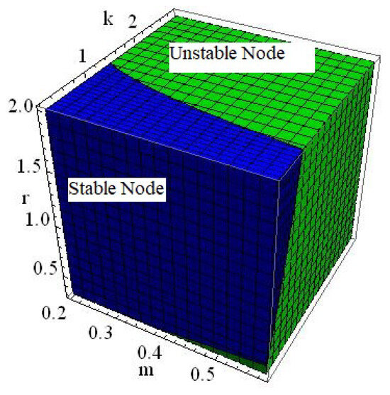
Lemma 6.
of the discrete model (6) is a stable node if , an unstable node if , and non-hyperbolic if
Proof.
Example 1.
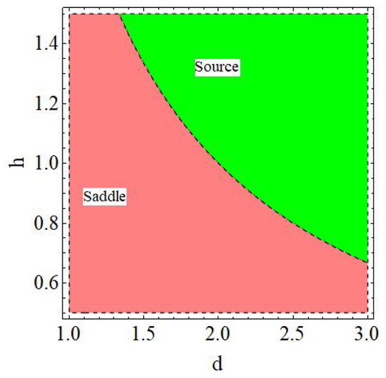
Figure 1.
Dynamics of where and .
Example 2.
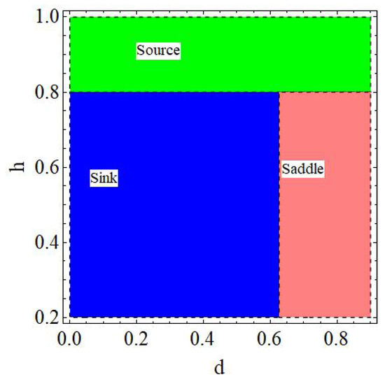
Figure 2.
Dynamics of where and .
Example 3.
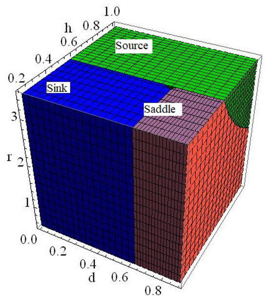
Figure 3.
Dynamics of where , and .
Example 4.
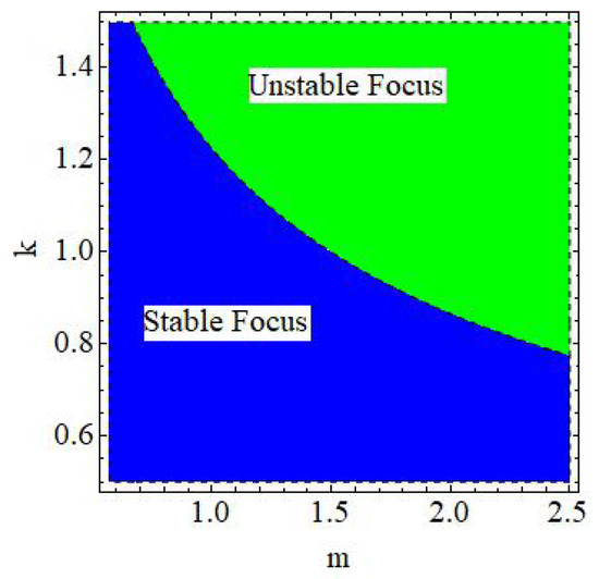
Figure 4.
Dynamics of where and .
Example 5.
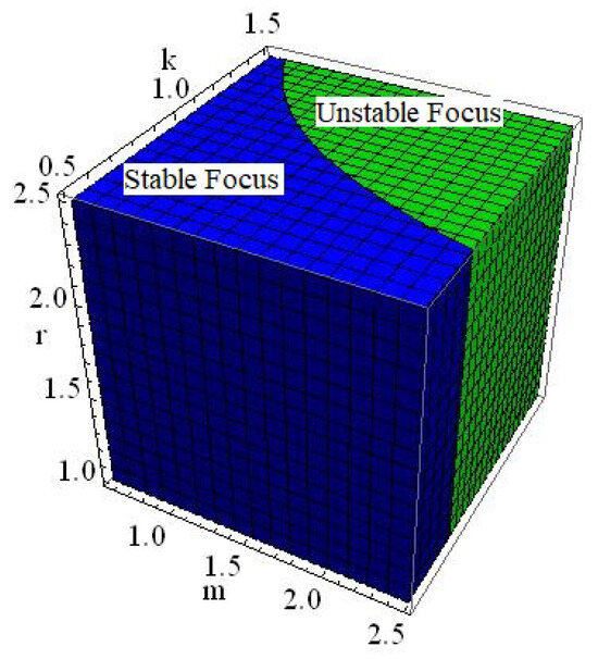
Figure 5.
Dynamics of where , and .
Example 6.
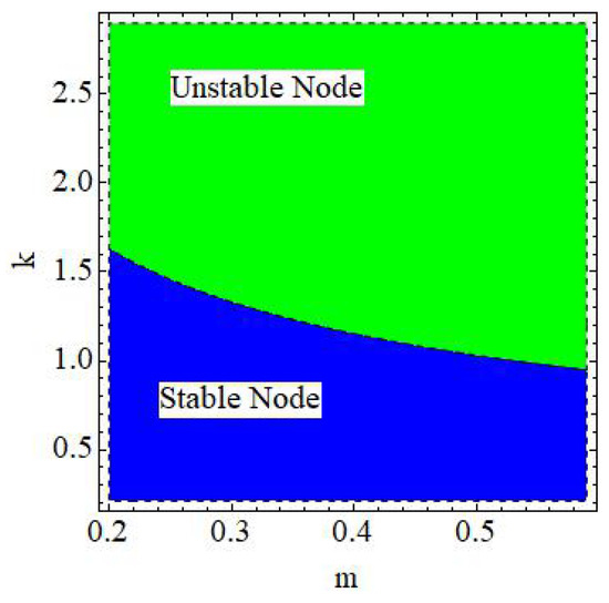
Figure 6.
Dynamics of where and .
3. Codimension-One Bifurcation
In this section, we give the comprehensive one-parameter bifurcations at , and of discrete model (6) using bifurcation theory [38,39,40,41,42,43,44,45,46,47].
3.1. Bifurcation at
If first condition of (20) holds then from (19) one gets but . This gives the fact that discrete model (6) may exhibit flip bifurcation if is located in the set:
Theorem 1.
At , discrete model (6) does not exhibit flip bifurcation if .
Proof.
If second condition of (20) holds then from (19) one gets but . This gives the fact that discrete model (6) may exhibit flip bifurcation if ℧ is located in the set:
Theorem 2.
At , discrete model (6) does not exhibit flip bifurcation if .
Proof.
Same as the proof of Theorem 1. □
3.2. Bifurcation at
Now, if (26) holds then which gives the fact that discrete model (6) may exhibit Neimark–Sacker bifurcation (NSB) if ℧ is located in the set:
Hereafter, if then we investigate NSB where m is regarded as a bifurcation parameter. So, the perturbation system of the discrete model (6) becomes
where and with . Furthermore, roots of evaluated at are
where and . Now, if then one has the conjugate complex roots satisfying , and subsequently, if (26) holds then one gets:
Moreover, for , the characteristics roots of (33) must not be found at the intersections of unit circle with coordinate axes. Therefore, one need to suppose that and for , which corresponds to . But if (26) holds then , and so . Therefore, , and so, by straightforward calculation one obtains , . Now, to transform , one uses the following transformations:
where (32), becomes
Now, normal form of (36) will be derived if . For this, from (36) the Taylor-series expansion up to second-order yields:
where
Now, by
(37) becomes
where its ingredients are shown in Appendix A. Now, from Appendix A, one gets , , , , , , , , , , , , , . Further, for the existence of NSB at of (40) following quantity must be nonzero:
where
So, (42) becomes
The above analysis yields the result:
Theorem 3.
Next, if the second condition of (27) holds, then from (24), one gets and , which implies that discrete model (6) may exhibit fold bifurcation if ℧ is located in the set:
Hereafter, we present in details fold bifurcation analysis if . So, if m changes behavior in a small neighborhood of , then by (35), discrete model (6) becomes
where
Now, by
(45) becomes
where
Now, center manifold theory, yields
where on calculation, one gets
Now, (48) corresponds to becomes
where
From, (52) and (53), one obtains
Finally, from (54), one gets , and which clearly violates the existence of fold bifurcation if . Hence, one has the conclusion:
Theorem 4.
At , discrete model (6) does not exhibit fold bifurcation if .
Finally, we will study flip bifurcation at of the discrete model (6). If first condition of (27) holds, then from (24), one gets , but , which implies that the discrete model (6) may exhibit flip bifurcation if ℧ is located in the set:
Hereafter, we will give detail analysis regarding the existence of flip bifurcation if . It is noted that (45) becomes the form:
where
by
Now, by center manifold theory, one writes
where its coefficients values are defined in Appendix B. Now, on expressing (56) restricted to , we have
where its coefficients values are also defined in Appendix B. Now, in order for (60) exhibits flip bifurcation, the following quantities require to be nonzero:
From, (60) and (61), one gets and So, the result is
Theorem 5.
At , the discrete model (6) exhibits flip bifurcation if where period-2 points bifurcate from are stable and an unstable if and , respectively.
4. Codimension-Two Bifurcations at
Now, we will examine the codimension-two bifurcation at of the discrete model (6) by existing theory [48,49,50]. From (23), one has
where
and
where
If , then from (64), one has with
and
Therefore, at , 2-parameter with 1:2 strong resonance bifurcation may exhibit if ℧ is located in the set:
Hereafter, the comprehensive 2-parameter with 1:2 resonance analysis is given. For this, if then from (36), one has
At , (69) takes the form
where
Now, from (70), if one denotes
then
where with . Furthermore, the straightforward calculation shows that corresponding to of , one has the following eigenvector
and generalized eigenvector
Similarly, eigenvector and generalized eigenvector of corresponding to , respectively are
and
Next, by calculation, quantities which are depicted in (74)–(77) satisfying the relation , , , , , and . Now, if
with then straightforward calculation yields
Now, in , (70) becomes
where
and
From (78), (81) and (82), the calculation yields
and
with . We define
with
(86) becomes
where
and
Now, if
then , So, (87) along with (88), (89) and (90) becomes
with
and
and . On utilizing
with
one has the 1:2 resonance normal form:
where
Finally, this theoretical analysis give the following result:
Theorem 6.
From (97), if and , then 1:2 strong resonance exists at . Furthermore, if (respectively, ), then is elliptic (respectively, saddle) and finally, near 1:2 point express the bifurcation curves:
- (i)
- Curve of Pitchfork bifurcationand additionally, for there exist nontrivial equilibrium state;
- (ii)
- Heteroclinic bifurcation curve:
- (iii)
- Non-degenerate N-S bifurcation curve:
- (iv)
- Homologous bifurcation curve:
Next, at of discrete model (6), 1:3 strong resonance is studied. If , then from (64), one gets, with
and
Therefore, at , 2-parameter with 1:3 strong resonance bifurcation may exhibit if ℧ is located in the set:
Further, in view of (104), (21) takes the form:
with with and are corresponding eigenvector and adjoint eigenvector of satisfying , , , and . Now, if where then (70) gives
where
with
and
Now, to eliminate quadratic terms from (106), one use the transformation:
wherever
with
Now, it is noted that if
then quadratic terms of (111) vanishes, and furthermore, cubic terms should be vanish by the transformation:
From (113) and (111), we obtain
where
On setting
Hence, the 1:3 resonance normal form is
where
Finally, if
then one has the following conclusion:
Theorem 7.
From (120), if and , then at , model (6) exhibits 2-parameter with 1:3 strong resonance bifurcation. Additionally, if , determine bifurcation behavior then at , model (6) consists the listed characteristics:
- (i)
- We have the non-degenerate Hopf bifurcation if (106) has the trivial fixed point;
- (ii)
- If (respectively, ) then 1:3 invariant closed curves appear which are unstable (respectively, stable).
- Finally, 2-parameter with 1:4 strong resonance is explore. If , then from (64), one gets, with
Theorem 8.
From (137), if and , then 1:4 strong resonance bifurcation exist at . Additionally, if determine the bifurcation then at , understudied model (6) has the listed dynamical characteristics:
- (i)
- There is a Hopf bifurcation at trivial fixed point of (133). Furthermore, if (respectively, ) then invariant circle appear (respectively, disappear);
- (ii)
- There are eight equilibrium points that disappear or appear in pairs via fold bifurcation if ;
- (iii)
- At eight fixed points, there is Hopf bifurcation.
Remark 2.
Remark 3.
Before study the chaos control for the discrete model (6), it is important here to mention that for certain parameter regimes, especially when the predation rate m is sufficiently small, the given discrete model (6) goes to decouples, and the prey equation reduces to a form of the classical logistic map, which is known to exhibit flip bifurcation, chaotic dynamics and other complex behaviors. To elaborate this, if one assume then from the discrete model (6), the iterative term in the first equation becomes negligible. In this case, the dynamics of decouple from and the prey dynamics approximate the discrete logistic map:
If one chooses then (138) becomes the form where it exhibits well-known chaotic dynamics when a is sufficiently large. Therefore, chaos in the system for small m values is not surprising. For more detail dynamical study for , we refer the reader to existing literature (see Page No. 52 of [51]). However, the focus of our study is not this limiting (decoupled) case, but rather the emergence of complex dynamics including chaos through codimension-one bifurcation: flip ad Neimark–Sacker bifurcations that arise as the parameters vary in the fully coupled discrete model (6). So, following section purely dedicated to examine the chaos using OGY and hybrid control strategies, which is not possible to investigate in the decoupled approximation. Our analysis thus provides a more comprehensive understanding for the discrete model (6) beyond the trivial decoupled case.
5. Chaos Control
We study the chaos by OGY and hybrid control strategies in the discrete model (6) based on existing theory [52,53]. It is important here to mention that necessity of designing a control algorithm arises from the fundamental observation that the original continuous model, which is depicted in (5), does not exhibit chaotic behavior, whereas its discretized version, obtained via Euler’s forward method, introduces complex dynamics including chaos. This divergence is significant because discretization though a standard numerical approach can qualitatively alter the system’s dynamics, potentially leading to undesirable or unpredictable behavior in simulations or real-world implementations. In the discrete model, chaos emerges through codimension-one bifurcations such as Neimark–Sacker and flip bifurcations. Therefore, to ensure the stability and predictability of the system, especially in biological or ecological applications, it becomes necessary to develop and implement control algorithms. The use of OGY and hybrid control strategies in this study serves this purpose by stabilizing chaotic trajectories near bifurcation points. This research approach is essential not only to understand the nature of chaos induced by discretization but also to provide practical solutions for maintaining ecological balance in modeled systems.
5.1. By OGY Method
We first use the OGY method in order to study chaos in the discrete model (6) where model is rewritten as
where c represents the control parameter under which one can acquire the desired chaos control by small perturbations. To do this, one restricts it where with , and indicates nominal value corresponds to chaotic region. The trajectory is moved in the direction of the target orbit using the stabilizing feedback control strategy. Assuming that if is an unstable fixed point of discrete model (6) within the chaotic region formed by NSB then following map can be used to approximate model (139):
where
and
Moreover, discrete model (139) is controlled provided that the following matrix
is of rank 2. To apply the OGY method to discrete model (139), one takes c as a control parameter. Now if one take , where , then model (140) can be written as
Furthermore, the corresponding controlled model of discrete model (139) is given by
By stability theory, is a sink iff roots of satisfying where its variational matrix is
with
If denotes the roots of (147) then
and
Next, we take and to get lines of marginal stability for (145) where these restrictions imply that . If then from (149), one has
Furthermore, if then from (148) and (149), one gets
and
Therefore, the lines which are depicted in (150)–(152) give the triangular region in -plane satisfying .
5.2. By Hybrid Control Strategy
Here, Hybrid control strategy is used to control the chaos due to emergence of flip bifurcation in (6) where it becomes
with . Now, for (153), one has
with
where
The above analysis gives the result:
Lemma 7.
of discrete model (153) is a stable .
6. Numerical Simulations
In this section, analytical findings will be confirmed numerically. All plots in this section will be drawn by the software Matlab R2014b/Mathematica 8. More importantly, the bifurcation diagrams presented in this section will be generated using refined numerical routines with a sufficiently small iteration step to ensure clarity and precision. The plotting approach follows the methodological guidance outlined by Jafari et al. [54], which enhances the accuracy and visual quality of the bifurcation structures. Furthermore, in these simulations, parametric values are carefully chosen to ensure that the necessary conditions, like non-hyperbolicity, eigenvalue criteria, and resonance conditions, are precisely satisfied. These parameter combinations are nontrivial to construct analytically and are essential to demonstrate the existence of NS, flip, and strong resonance bifurcations.
Example 8.
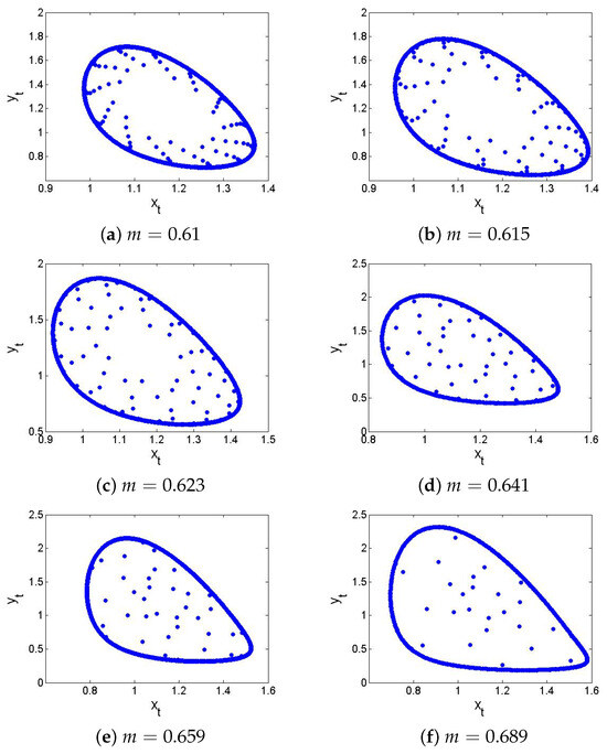
If , , , , then from the non-hyperbolic condition (26), one gets . Now, if , , , , , and then from (24) one has , which satisfies the eigenvalues criterion for the existence of NSB at of the model (6), and hence, from (31) one gets . Next, in order to ensure the theoretical conclusion of Lemma 5 numerically, Figure 8 and Figure 9 show that the respective is a stable (respectively, unstable) focus if (respectively ). The existence of an unstable focus implies that there must appear the stable curves, and in fact, at , the discrete model (6) exhibits supercritical NSB if , that is, from (41), one has . In order to prove this, if , then from (43), one gets
Using and (157) in (41) one gets , which coincides with the conclusion of Theorem 3. Finally, NSB diagrams with maximum Lyapunov exponents are sketched and displayed in Figure 10. In summary, at , of the model (6) transits from stable to an unstable via N-S bifurcation, leading to the emergence of closed invariant curves. Biologically, this transition reflects a shift from steady-state coexistence of prey and predator to stable population oscillations such as periodic outbreaks. Furthermore, if the predator growth rate m increases slightly beyond the critical value, that is, , then the discrete model (6) cannot stabilize at equilibrium, and ecological cycles emerges a well-documented phenomenon in many real predator–prey systems such as lynx-hare dynamics.
Figure 8.
Phase portrait of the discrete model (6) if .
Figure 9.
Phase portrait of the discrete model (6) if .
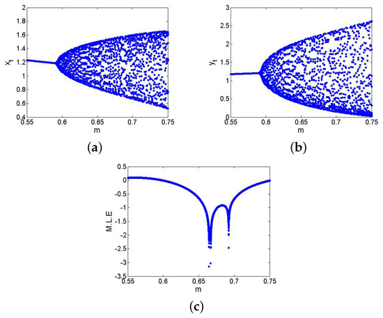
Figure 10.
NSB diagrams and MLE of the discrete model (6) where . (a) for ; (b) for ; (c) MLE.
Example 9.
If , , , , and , then from (27), one gets . Furthermore, if , , , , , and , then from (24), one gets and , which satisfies eigenvalues criterion; hence, from (55), one has . Finally, the straightforward Mathematica calculation is performed if , where from (61), one gets and which holds the conclusion of Theorem 5. Hence, flip bifurcation diagram with MLE are sketched and represented in Figure 11. In summary, the flip bifurcation occurs at with one eigenvalue . Biologically, the occurrence of flip bifurcation at implies that the predator and prey populations begin to alternate periodically—a hallmark of predator–prey interactions under certain resource constraints. The doubling of cycles is often observed in seasonal or annual prey–predator systems, where over-predation in one generation leads to scarcity and subsequent collapse, followed by recovery.
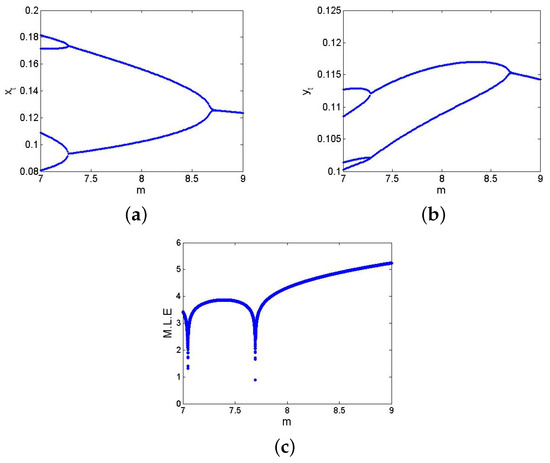
Figure 11.
FB and MLE of discrete model (6) if . (a) for ; (b) for ; (c) MLE.
Example 10.
If , , , and , then from (66) and (67), one gets and . Furthermore, for said parametric values, discrete model (6) has a fixed point , where from (64), one gets ; hence, for the existence of 2-parameter bifurcation with 1:2 strong resonance, the eigenvalues criterion holds. Therefore, from (68), the set . But from (97), the calculation yields that , , and , which satisfies the conclusion of Theorem 6; the respective bifurcation diagrams are depicted in Figure 12. Biologically, the occurrence of 1:2 bifurcation suggests a system with strong two-period oscillations. Such behavior might correspond to ecosystems where reproductive cycles renewals happen every two time units, and predator–prey interactions synchronize with these cycles, resulting in alternations among low and high densities every two periods.
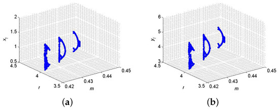
Figure 12.
2-parameter with 1:2 resonance bifurcation diagram at . (a) for ; (b) for .
Example 11.
If , , , and then from (102) and (103) one gets and . Furthermore, for said parametric values, discrete model (6) has fixed point where from (64) one gets , and hence, for the existence of 2-parameter bifurcation with 1:3 strong resonance the eigenvalues criterion holds. Therefore, the set . But from (119), one gets and . Finally, from (120) one gets and where imply that at , model (6) exhibits 1:3 strong resonance bifurcation which satisfies the conclusion of Theorem 7, and so, the respective diagrams are sketched in Figure 13. Biologically, occurrence of 1:3 resonance leads to triply periodic cycles, indicating possible multi-annual oscillatory patterns in species interactions. This type of dynamics might be relevant in complex food webs where predator foraging behavior or prey reproduction occurs in 3-year intervals.
Figure 13.
2-parameter with 1:3 resonance bifurcation diagram at . (a) for ; (b) for .
Example 12.
If , , , and then from (121) and (122) one gets and . Furthermore, for said parametric values, discrete model (6) has fixed point where from (64), one gets , and hence, the eigenvalues criterion holds for the existence of 2-parameter bifurcation with 1:4 strong resonance. Therefore, the set . But from (134), one gets , and . Now, from (135), one gets and . Finally, from (137), we have , where and , which imply that at , discrete model (6) exhibits 1:4 strong resonance bifurcation that satisfies the conclusion of Theorem 8; the respective diagrams are sketched in Figure 14. Biologically, 1:4 strong resonance dynamics are associated with quasi-periodic or complex cycles that repeat every four generations. These might model biological systems where external environmental pressures such as climate cycles or disease act on a 4-year rhythm, influencing the predator–prey dynamics accordingly.
Figure 14.
2-parameter with 1:4 resonance bifurcation diagram at . (a) for ; (b) for .
Example 13.
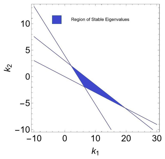
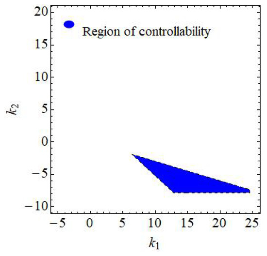
If , , , , , then from (150)–(152) one gets: , and where these three lines formed the triangular (see Figure 15). Furthermore, if , , , , , and varying , then region of controllability in 2D is given in Figure 16. Finally, if , , , , , and varying and then region of controllability in 3D is given in Figure 17.
Figure 15.
Region of stability where .
Figure 16.
Region of controllability if , , , , and and varying of (145).
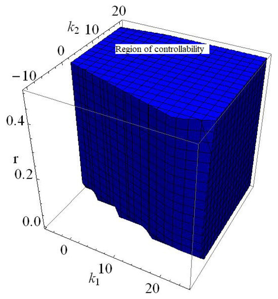
Figure 17.
Region of controllability if , , , and and varying and of (145).
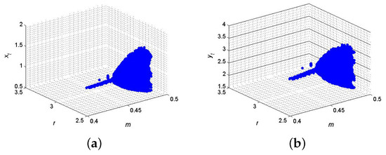
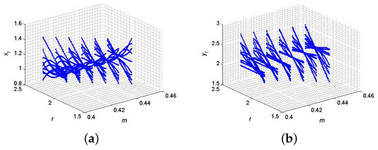
Example 14.
Finally, if one reconsider the data from Example 9 with then phase portrait of controlled model (153) is given in Figure 18 whereas regions of controllability in 2D and 3D are presented in Figure 19 and Figure 20, respectively.
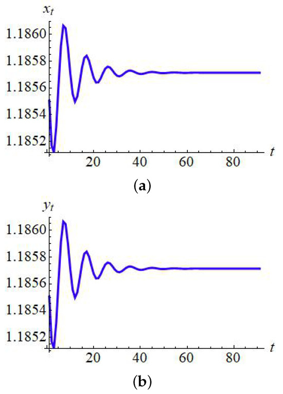
Figure 18.
Phase portrait for (153) with and . (a) for ; (b) for .
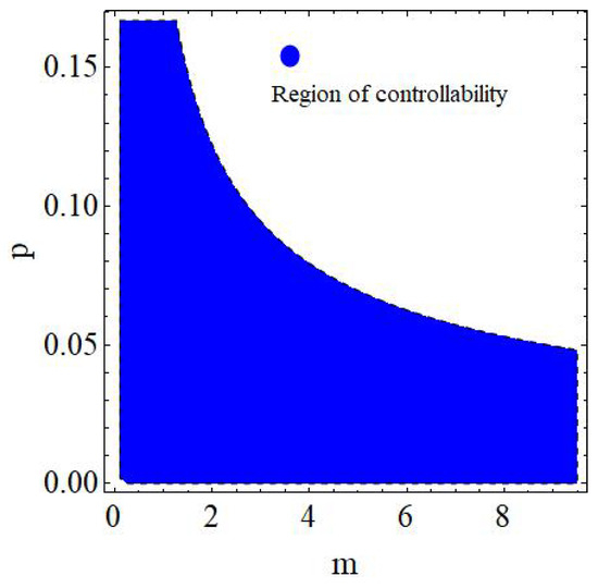
Figure 19.
Region of controllability in 2D of (153) by varying and .
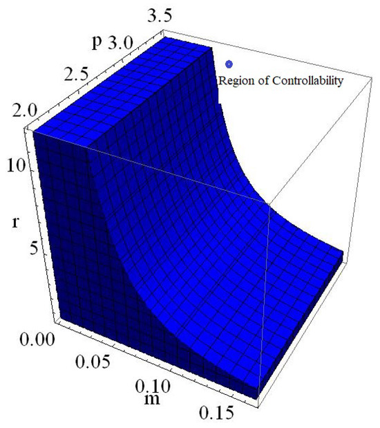
Figure 20.
Phase portrait in 3D of (153) by varying , and .
7. Conclusions
We explored fixed points, local behavior, and codimension-one and two bifurcations of a discrete model with Holling type I functional response, which is depicted in (6). It is proved that for all c, d, h, k, m, and r, discrete model (6) has a TFP along with two BFPs and , and moreover, if , then it has an IFP . We then first constructed the linearized system at TFP, two BFPs and IFP, and then based on linearized system local behavior by linear stability theory is explored. It is proved that is never sink but source, saddle and non-hyperbolic if , and , respectively, and is never sink, source, saddle but it is non-hyperbolic if . Further, it is examined that if , , or and or then is a sink, source, saddle, and non-hyperbolic, respectively. Finally, regarding local dynamics, it is also examined that is a stable focus, unstable, and non-hyperbolic if , and , and also it is stable node, unstable node, and non-hyperbolic if , and or , respectively. Next, for further understanding of the complex behavior of the discrete model (6), we studied the 1 and 2-parameter bifurcations and proved that at (i) , no flip bifurcation exists if , and , and (ii) 1-parameter bifurcation, namely NSB and flip bifurcations, both exist at if and , but at this point no fold bifurcation exists if . Furthermore, we also studied the 2-parameter bifurcations at , and examined that 2-parameter with 1:2, 1:3, and 1:4 resonance bifurcations exist if and , respectively. Further, we also studied the chaos by OGY and hybrid strategies due to the appearance of 1-parameter bifurcation: NSB and flip bifurcation, respectively. Finally, theoretical results are validated numerically. In conclusion, the results of our study provide important insights into the complex behavior of a discrete model (6) with asymmetric interactions—an area of ecological modeling that reflects more realistic inter-species relationships in nature. More specifically, the identification of codimension-one bifurcations: N-S and flip bifurcations at helps us in order to understand the mechanisms through which population cycles and chaotic dynamics can emerge in real biological systems. Furthermore, the study of codimension-two strong resonance bifurcations such as 1:2, 1:3, and 1:4 offers a deeper understanding of how small changes in parameters can lead to sudden qualitative changes in the system’s behavior, which is critical in the control and management of ecological populations. Finally, the application of OGY and hybrid control strategies due to the appearance of NSB and flip bifurcations, respectively, provides a practical interpretation that could be useful for the resource management.
Future Work and Extension
Calculating the forbidden set and analyzing the global dynamics of the discrete model (6) will focus of our future work. Additionally, we plan to extend this research by conducting a comprehensive dynamical analysis of a three-species prey–predator model, which will offer deeper insights into the complex interactions within multi-species ecosystems.
Author Contributions
Conceptualization, M.R.R., A.Q.K. and J.G.A.-J.; Methodology, M.R.R. and A.Q.K.; Software, M.R.R. and A.Q.K.; Validation, A.Q.K.; Formal analysis, M.R.R., A.Q.K. and J.G.A.-J.; Investigation, M.R.R., A.Q.K. and J.G.A.-J.; Resources, J.G.A.-J.; Writing—original draft, M.R.R., A.Q.K. and J.G.A.-J.; Writing—review & editing, M.R.R., A.Q.K. and J.G.A.-J.; Visualization, A.Q.K.; Supervision, A.Q.K.; Funding acquisition, J.G.A.-J. All authors have read and agreed to the published version of the manuscript.
Funding
The authors would like to acknowledge Deanship of Graduate Studies and Scientific Research, Taif University for funding this work.
Data Availability Statement
No new data were created or analyzed in this study. Data sharing is not applicable to this article.
Acknowledgments
The authors would like to acknowledge Deanship of Graduate Studies and Scientific Research, Taif University for funding this work.
Conflicts of Interest
The authors declare that they have no conflict of interest regarding the publication of the paper.
Appendix A. Representation of Ingredients of (40)
Appendix B. Representation of Ingredients of (59)
References
- Murray, J.D. Mathematical Biology: An Introduction; Springer Science & Business Media: Berlin/Heidelberg, Germany, 2007. [Google Scholar]
- Britton, F.N. Essential Mathematical Biology; Springer Science & Business Media: Berlin/Heidelberg, Germany, 2012. [Google Scholar]
- Lotka, A.J. Elements of Physical Biology; Williams, & Wilkins: Philadelphia, PA, USA, 1925. [Google Scholar]
- Volterra, V. Fluctuations in the abundance of a species considered mathematically. Nature 1926, 118, 558–560. [Google Scholar] [CrossRef]
- Holling, C.S. The components of predation as revealed by a study of small-mammal predation of the European pine sawfly. Can. Entomol. 1959, 91, 293–320. [Google Scholar] [CrossRef]
- Rosenzweig, M.L.; MacArthur, R.H. Graphical representation and stability conditions of predator-prey interactions. Am. Nat. 1963, 97, 209–223. [Google Scholar] [CrossRef]
- May, R.M. Simple mathematical models with very complicated dynamics. Nature 1976, 261, 459–467. [Google Scholar] [CrossRef]
- Khan, A.Q.; Akhtar, T.; Jhangeer, A.; Riaz, M.B. Codimension-two bifurcation analysis at an endemic equilibrium state of a discrete epidemic model. Aims Math. 2024, 9, 13006–13027. [Google Scholar] [CrossRef]
- Govaerts, W.; Kuznetsov, Y.A.; Ghaziani, R.K.; Meijer, H.G.E. Cl Matcontm: A Toolbox for Continuation and Bifurcation of Cycles of Maps; Universiteit Gent: Gent, Belgium; Utrecht University: Utrecht, The Netherlands, 2008. [Google Scholar]
- Chen, Q.; Teng, Z. Codimension-two bifurcation analysis of a discrete predator–prey model with nonmonotonic functional response. J. Differ. Equations Appl. 2017, 23, 2093–2115. [Google Scholar] [CrossRef]
- Arancibia–Ibarra, C.; Flores, J. Dynamics of a Leslie–Gower predator–prey model with Holling type-II functional response, Allee effect and a generalist predator. Math. Comput. Simul. 2021, 188, 1–22. [Google Scholar] [CrossRef]
- Chen, L.; Chen, F.; Chen, L. Qualitative analysis of a predator–prey model with Holling type-II functional response incorporating a constant prey refuge. Nonlinear Anal. Real World Appl. 2010, 11, 246–252. [Google Scholar] [CrossRef]
- Pusawidjayanti, K.; Kusumasari, V. Dynamical analysis predator-prey population with Holling type-II functional response. J. Phys. Conf. Ser. 2021, 1872, 012035. [Google Scholar] [CrossRef]
- Sambath, M.; Balachandran, K.; Surendar, M.S. Functional responses of prey-predator models in population dynamics: A Survey. J. Appl. Nonlinear Dyn. 2024, 13, 83–98. [Google Scholar] [CrossRef]
- Shang, Z.; Qiao, Y.; Duan, L.; Miao, J. Bifurcation analysis in a predator-prey system with an increasing functional response and constant-yield prey harvesting. Math. Comput. Simul. 2021, 190, 976–1002. [Google Scholar] [CrossRef]
- Naik, P.A.; Eskandari, Z.; Yavuz, M.; Huang, Z. Bifurcation results and chaos in a two-dimensional predator-prey model incorporating Holling type response function on the predator. Discret. Contin. Dyn. Syst.-S 2024, 18, 1212–1229. [Google Scholar] [CrossRef]
- Mandal, G.; Rojas-Palma, A.; González-Olivares, E.; Chakravarty, S.; Guin, L.N. Allee-induced periodicity and bifurcations in a Gause-type model with interference phenomena. Eur. Phys. J. B 2025, 98, 63. [Google Scholar] [CrossRef]
- Khan, A.Q.; Alsulami, I.M. Complicate dynamical analysis of a discrete predator-prey model with a prey refuge. Aims Math. 2023, 8, 15035–15057. [Google Scholar] [CrossRef]
- Al-Kaff, M.O.; AlNemer, G.; El-Metwally, H.A.; Elsadany, A.E.A.; Elabbasy, E.M. Dynamic behavior and bifurcation analysis of a modified reduced Lorenz model. Mathematics 2024, 12, 1354. [Google Scholar] [CrossRef]
- Cai, Y.; Chen, Q.; Teng, Z.; Zhang, G.; Rifhat, R. Bifurcations in a discrete-time Beddington-DeAngelis prey-predator model with fear effect, prey refuge and harvesting. Nonlinear Dyn. 2025, 113, 931–969. [Google Scholar] [CrossRef]
- Wu, X.; Zhou, Z.; Xie, F. Multi-scale dynamics of a piecewise-smooth Bazykin’s prey-predator system. Nonlinear Dyn. 2025, 113, 1969–1981. [Google Scholar] [CrossRef]
- Torkzadeh, L.; Fahimi, M.; Ranjbar, H.; Nouri, K. Analysis of a stochastic model for a prey-predator system with an indirect effect. Int. J. Comput. Math. 2025, 102, 60–73. [Google Scholar] [CrossRef]
- Yao, J.; Huang, J.; Wang, H. Relaxation oscillation, homoclinic orbit and limit cycles in a piecewise smooth predator-prey model. Qual. Theory Dyn. Syst. 2024, 23, 289. [Google Scholar] [CrossRef]
- Zhang, H.; Cai, Y.; Shen, J. Super-explosion and inverse canard explosion in a piecewise-smooth slow-fast Leslie-Gower model. Qual. Theory Dyn. Syst. 2024, 23, 73. [Google Scholar] [CrossRef]
- Tian, Y.; Zhu, J.; Zheng, J.; Sun, K. Modeling and analysis of a prey-predator system with prey habitat selection in an environment subject to stochastic disturbances. Electron. Res. Arch. 2025, 33, 744–767. [Google Scholar] [CrossRef]
- Das, S.; Chatterjee, A.N.; Rana, S. Complex dynamics of a discrete time one prey two predator system with prey refuge. Int. J. Appl. Comput. Math. 2025, 11, 86. [Google Scholar] [CrossRef]
- Mokni, K.; Ch-Chaoui, M. Dynamic analysis and chaos control in a discrete predator-prey model with Holling type-IV and nonlinear harvesting. Miskolc Math. Notes 2024, 25, 899–919. [Google Scholar] [CrossRef]
- Li, S.; Wang, X.; Li, X.; Wu, K. Relaxation oscillations for Leslie-type predator–prey model with Holling type-I response functional function. Appl. Math. Lett. 2021, 120, 107328. [Google Scholar] [CrossRef]
- Liu, B.; Zhang, Y.; Chen, L. Dynamic complexities of a Holling I predator–prey model concerning periodic biological and chemical control. Chaos Solitons Fractals 2004, 22, 123–134. [Google Scholar] [CrossRef]
- Ruan, M.J.; Li, C.; Li, X.Y. Codimension two 1:1 strong resonance bifurcation in a discrete predator-prey model with Holling IV functional response. Aims Math. 2021, 7, 3150–3168. [Google Scholar] [CrossRef]
- Lampert, W. Release of dissolved organic carbon by grazing zooplankton. Limnol. Oceanogr. 1978, 23, 831–834. [Google Scholar] [CrossRef]
- Murdoch, W.W.; Oaten, A. Predation and population stability. Adv. Ecol. Res. 1975, 9, 1–131. [Google Scholar]
- Camouzis, E.; Ladas, G. Dynamics of Third-Order Rational Difference Equations with Open Problems and Conjectures; Chapman and Hall/CRC: Boca Raton, FL, USA, 2007. [Google Scholar]
- Grove, E.A.; Ladas, G. Periodicities in Nonlinear Difference Equations; Chapman & Hall/CRC: Boca Raton, FL, USA, 2004. [Google Scholar]
- Kocic, V.L.; Ladas, G. Global Behavior of Nonlinear Difference Equations of Higher-Order with Applications; Springer Science & Business Media: Berlin/Heidelberg, Germany, 1993. [Google Scholar]
- Sedaghat, H. Nonlinear Difference Equations: Theory with Applications to Social Science Models; Springer Science & Business Media: Berlin/Heidelberg, Germany, 2013. [Google Scholar]
- Wikan, A. Discrete Dynamical Systems with an Introduction to Discrete Optimization Problems; Bookboon. com: London, UK, 2013. [Google Scholar]
- Guckenheimer, J.; Holmes, P. Nonlinear Oscillations, Dynamical Systems, and Bifurcations of Vector Fields; Springer Science & Business Media: Berlin/Heidelberg, Germany, 2013. [Google Scholar]
- Kuznetsov, Y.A. Elements of Applied Bifurcation Theorey; Springer: New York, NY, USA, 2004. [Google Scholar]
- Gümüşboga, F.; Kangalgil, F. Dynamics of a discrete predator–prey model with an Allee effect in prey: Stability, bifurcation analysis and chaos control. Int. J. Bifurc. Chaos 2025, 35, 2550097. [Google Scholar] [CrossRef]
- Su, X.; Wang, J.; Bao, A. Stability analysis and chaos control in a discrete predator-prey system with Allee effect, fear effect, and refuge. Aims Math. 2024, 9, 13462–13491. [Google Scholar] [CrossRef]
- Jia, C.; Wang, J.; Zhang, J.F. A predator–prey model: Understanding the role of fear effect. Int. J. Bifurc. Chaos 2025, 35, 2550092. [Google Scholar] [CrossRef]
- Lv, L.; Li, X. Stability and bifurcation analysis in a discrete predator–prey system of Leslie-type with radio-dependent simplified Holling type-IV functional response. Mathematics 2024, 12, 1803. [Google Scholar] [CrossRef]
- Hong, B.; Zhang, C. Neimark–Sacker bifurcation of a discrete-time predator–prey model with prey refuge effect. Mathematics 2023, 11, 1399. [Google Scholar] [CrossRef]
- Sardar, P.; Biswas, S.; Das, K.P.; Rana, S.; Pal, B.; Ali, M.F.; Gupta, V. Exploring multiple bifurcation behaviors and chaos control via weak Allee effect and harvesting in a predator-prey interaction model. Nonlinear Sci. 2025, 4, 100033. [Google Scholar] [CrossRef]
- Singh, A.; Deolia, P. Bifurcation and chaos in a discrete predator–prey model with Holling type-III functional response and harvesting effect. J. Biol. Syst. 2021, 29, 451–478. [Google Scholar] [CrossRef]
- Ara, R.; Sohel Rana, S.R. Complex dynamics and chaos control of discrete prey–predator model with caputo fractional derivative. Complexity 2025, 2025, 4415022. [Google Scholar] [CrossRef]
- Li, Y.; Liu, L.; Chen, Y.; Yu, Z. Bifurcations and Marotto’s chaos of a discrete Lotka–Volterra predator–prey model. Phys. Nonlinear Phenom. 2025, 472, 134524. [Google Scholar] [CrossRef]
- Liu, M.; Ma, L.; Hu, D. Some bifurcations of codimensions 1 and 2 in a discrete predator–prey model with non-linear harvesting. Mathematics 2024, 12, 2872. [Google Scholar] [CrossRef]
- Lei, C.; Han, X. Codimension-two bifurcation analysis of a discrete predator–prey system with fear effect and Allee effect. Nonlinear Anal. Model. Control. 2025, 30, 386–404. [Google Scholar] [CrossRef]
- Allen, L.J. Introduction to Mathematical Biology; Pearson/Prentice Hall: London, UK, 2007. [Google Scholar]
- Elaydi, S. An Introduction to Difference Equations; Springer: New York, NY, USA, 1996. [Google Scholar]
- Lynch, S. Dynamical Systems with Applications Using Mathematica; Birkhäuser: Boston, MA, USA, 2007. [Google Scholar]
- Jafari, A.; Hussain, I.; Nazarimehr, F.; Golpayegani, S.M.R.H.; Jafari, S. A simple guide for plotting a proper bifurcation diagram. Int. J. Bifurc. Chaos 2021, 31, 2150011. [Google Scholar] [CrossRef]
Disclaimer/Publisher’s Note: The statements, opinions and data contained in all publications are solely those of the individual author(s) and contributor(s) and not of MDPI and/or the editor(s). MDPI and/or the editor(s) disclaim responsibility for any injury to people or property resulting from any ideas, methods, instructions or products referred to in the content. |
© 2025 by the authors. Licensee MDPI, Basel, Switzerland. This article is an open access article distributed under the terms and conditions of the Creative Commons Attribution (CC BY) license (https://creativecommons.org/licenses/by/4.0/).