A System of Parabolic Laplacian Equations That Are Interrelated and Radial Symmetry of Solutions

Abstract

We utilize the moving planes technique to prove the radial symmetry along with the monotonic characteristics of solutions for a system of parabolic Laplacian equations. In this system, the solutions of the two equations are interdependent, with the solution of one equation depending on the function of the other. By use of the maximal regularity theory that has been established for fractional parabolic equations, we ensure the solvability of these systems. Our initial step is to formulate a narrow region principle within a parabolic cylinder. This principle serves as a theoretical basis for implementing the moving planes method. Following this, we focus our attention on parabolic systems with fractional Laplacian equations and deduce that the solutions are radial symmetric and monotonic when restricted to the unit ball.

1. Introduction

This paper sets out to examine a system of parabolic Laplacian equations within the unit ball

$$\begin{array}{c}\hfill \left\{\begin{array}{c}{\displaystyle \frac{\partial u}{\partial t}}+{(-\Delta )}^{{\displaystyle \frac{\alpha }{2}}}u(x,t)=f\left(v(x,t)\right),\hfill \\ {\displaystyle \frac{\partial v}{\partial t}}+{(-\Delta )}^{{\displaystyle \frac{\beta }{2}}}v(x,t)=g\left(u(x,t)\right),\hfill \end{array}\right.\end{array}$$

with

$$\begin{array}{cc}{(-\Delta )}^{s}u(x,t)\hfill & \equiv C_{n,s}P.V.{\int }_{{\mathbb{R}}^n}{\displaystyle \frac{u(x,t)-u(y,t)}{{|x-y|}^{n+2s}}}dy\hfill \\ & \equiv C_{n,s}\underset{\epsilon \to 0^{+}}{\lim }{\int }_{{\mathbb{R}}^n\setminus B_{\epsilon }\left(x\right)}{\displaystyle \frac{u(x,t)-u(y,t)}{{|x-y|}^{n+2s}}}dy,\hfill \end{array}$$

(1)

provided that s is a real number and $0<s<1$, $C_{n,s}$ serves as a positive normalization constant, the value of which is determined by n and s. Meanwhile, $P.V.$ indicates the Cauchy Principal value.

For the integral to be well-defined in (1), we stipulate that $u\in {\mathcal{L}}_{2s}\cap C_{loc}^{1,1}$, where the function u also satisfies

$$\begin{array}{c}\hfill {\mathcal{L}}_{2s}\equiv \left\{u:{\mathbb{R}}^n\to \mathbb{R}|{\int }_{{\mathbb{R}}^n}{\displaystyle \frac{\left|u\right(x,t\left)\right|}{1+{\left|x\right|}^{n+2s}}}dx<+\infty \right\}.\end{array}$$

Unlike local differential operators, the fractional Laplacian is nonlocal, integrating global information to define its value at a point. This nonlocality has made it a cornerstone in modeling nonlocal phenomena, sparking widespread research interest in fractional Laplacian equations [1,2,3,4,5,6,7]. The inherent nonlocality of the fractional Laplacian presents a formidable barrier to its study. To overcome these difficulties, the moving plane method has turned out to be a key way for looking into the qualitative features of solutions to equations with nonlocal operators. For further references, see [8,9,10].

In our paper, we use the direct moving plane method to investigate the radial symmetry and monotonic characteristics of solutions of parabolic Laplacian systems. A. D. Alexandrov originally put forward the renowned moving plane method to prove the Soap Bubble Theorem as mentioned in [11]. From the moment it was initially proposed, the moving plane method has undergone significant refinements and extensions by various mathematicians, among whom Serrin’s work in 1971 [12] stands as a notable milestone. Later on, a direct moving plane method was developed by Chen et al. [10]; researchers used it in many applications, such as deriving monotonic, one-dimensional symmetric solutions of equations and systems involving fractional Laplacian operators [13,14,15,16].

Liu (2025) [7] employed the direct moving plane method to prove the radial symmetric and monotonic solutions of parabolic fractional Laplacian equations; we generalize those results on fractional parabolic systems. In this system, the parabolic Laplacian operator related to u is related to the function related to v, and the parabolic Laplacian operator related to v is related to the function related to u, which has increased the complexity of the system; more contents related with fractional parabolic systems and constraint conditions on fractional parabolic systems can be seen in [17]. We aim to prove that the solutions of the fractional parabolic equations in this system are radial symmetric and monotone. We adopt the setting in [7], where u only converges almost everywhere; this setting is an alternative or innovation to the method of setting a bound for u and making sure that u is uniformly convergent. Based on the underlying logic of maximum regularity in [18], we indirectly regulate the fractional Laplacian operator based on convergent conditions of u and v, thus managing the eigenvalue of fractional Laplacian operator to ensure the existence of solutions. Next, we use the direct moving plane method to prove this kind of fractional parabolic system, thanks to the radial symmetric and monotonic solutions.

2. Main Results

For this kind of parabolic Laplacian system which is interrelated, our goal was to prove the following significant theorems:

Theorem 1. 

Let $B_1\left(0\right)$ be a unit ball. Let $0<\alpha ,\beta <2$ and suppose that $u(x,t),v(x,t)\in \left(C_{loc}^{1,1}\left(B_1\left(0\right)\right)\cap C\left(\overline{B_1\left(0\right)}\right)\right)\times \mathbb{R}$ are positive bounded classical solutions of

$$\begin{array}{c}\hfill \left\{\begin{array}{cc}{\displaystyle \frac{\partial u}{\partial t}}+{(-\Delta )}^{{\displaystyle \frac{\alpha }{2}}}u(x,t)=f\left(v(x,t)\right),\hfill & (x,t)\in B_1\left(0\right)\times \mathbb{R},\hfill \\ {\displaystyle \frac{\partial v}{\partial t}}+{(-\Delta )}^{{\displaystyle \frac{\beta }{2}}}v(x,t)=g\left(u(x,t)\right),\hfill & (x,t)\in B_1\left(0\right)\times \mathbb{R},\hfill \\ u(x,t)\stackrel{a.e.}{\to }{u}_0(x,t)>0,\hfill & (x,t)\in B_1\left(0\right)\times \mathbb{R},\hfill \\ v(x,t)\stackrel{a.e.}{\to }{v}_0(x,t)>0,\hfill & (x,t)\in B_1\left(0\right)\times \mathbb{R},\hfill \\ u(x,t),v(x,t)\equiv 0,\hfill & x\notin B_1\left(0\right),\hfill \end{array}\right.\end{array}$$

(2)

and assume that $f\left(v\right(x,t\left)\right),g\left(u\right(x,t\left)\right)$ satisfy the following assumptions:

(M1) $f(·)$ is non-decreasing in $v(·)$, and $g(·)$ is non-decreasing in $u(·)$.

(M2) f and g are characterized by uniform Lipschitz continuity with regard to the variables u and v, i.e.:

$$\begin{array}{c}\hfill |f\left(v_1\right)-f\left(v_2\right)|\le c|v_1-v_2|,\\ \hfill |g\left(u_1\right)-f\left(u_2\right)|\le c|u_1-u_2|.\end{array}$$

Then, the functions $u(x,t)$ and $v(x,t)$ exhibit radial symmetry with respect to the origin and demonstrate a monotone decreasing behavior as they move away from the origin.

Remark 1. 

The notation $u(x,t)\stackrel{a.e.}{\to }{u}_0(x,t)$ and $v(x,t)\stackrel{a.e.}{\to }{v}_0(x,t)$ signify that $u(x,t)$ converges almost everywhere to $u_0(x,t)$ and $v(x,t)$ converges almost everywhere to $v_0(x,t)$ for $(x,t)\in B_1\left(0\right)\times \mathbb{R}$. In our specific context, within a measure space $(X,\mathrm{\Sigma },\mu )$ where $\mathrm{\Sigma }\subset B_1\left(0\right)$, there exist sequences of functions $\left\{u_n\right\}$ and $\left\{v_n\right\}$ along with functions u and v, such that for any $\epsilon >0$, there exists a set $E\in \mathrm{\Sigma }$ with $\mu \left(E\right)<\epsilon$. For all $x\in X\setminus E$, we have $u_n(x,t)\to u(x,t)$ and $v_n(x,t)\to v(x,t)$. This implies that $u_n$ and $v_n$ converge to u and v at all points except those in a set of measure zero. The rationale behind imposing this condition will be elaborated upon in Section 3.

Theorem 1, which was cited in [19], has been enhanced compared to its counterpart in [19]. The enhancement involved the addition of convergent conditions on the variables u and v, making the theorem more comprehensive.

To streamline the notation, we shall henceforth represent $U_{\lambda }$ as U, $V_{\lambda }$ as V, ${\mathrm{\Sigma }}_{\lambda }$ as $\mathrm{\Sigma }$, and ${\mathrm{\Omega }}_{\lambda }$ as $\mathrm{\Omega }$ to prove the subsequent Theorem; Theorem 2 is cited in [19].

Theorem 2. 

(Narrow region principle on a parabolic cylinder). Let $\mathrm{\Omega }\times (\underline{t},T]$ be a bounded region in $\mathrm{\Sigma }\times (\underline{t},T]$, such that for λ sufficiently close to $-1$, $\mathrm{\Omega }\times (\underline{t},T]$ is a bounded narrow region. For $0<\alpha ,\beta <2$, assume that $U(x,t)\in [C_{loc}^{1,1}\left(\mathrm{\Omega }\right)\cap C\left(\overline{\mathrm{\Omega }}\right)\cap {\mathcal{L}}_{\alpha }]\times C^1\left([\underline{t},T]\right)$, $V(x,t)\in [C_{loc}^{1,1}\left(\mathrm{\Omega }\right)\cap C\left(\overline{\mathrm{\Omega }}\right)\cap {\mathcal{L}}_{2s}]\times C^1\left([\underline{t},T]\right)$, and $U(x,t)$, $V(x,t)$ are lower semi-continuous on $\overline{\mathrm{\Omega }}\times [\underline{t},T]$. If $c_i(x,t)\ge 0$, $i=1,2$ are bounded from below in $\mathrm{\Omega }\times (\underline{t},T]$ and $c_i(x,t)$ are Lipschitz continuous, and

$$\begin{array}{c}\hfill \left\{\begin{array}{cc}{\displaystyle \frac{\partial U}{\partial t}}+{(-\Delta )}^{{\displaystyle \frac{\alpha }{2}}}U(x,t)\ge c_{1}V(x,t),\hfill & (x,t)\in \mathrm{\Omega }\times [\underline{t},T],\hfill \\ {\displaystyle \frac{\partial V}{\partial t}}+{(-\Delta )}^{{\displaystyle \frac{\beta }{2}}}V(x,t)\ge c_{2}U(x,t),\hfill & (x,t)\in \mathrm{\Omega }\times [\underline{t},T],\hfill \\ U(x,t),V(x,t)\ge 0,\hfill & (x,t)\in \mathrm{\Sigma }\setminus \mathrm{\Omega }\times [\underline{t},T],\hfill \\ U(x^{\lambda },t)=-U(x,t),\hfill & (x,t)\in \mathrm{\Sigma }\times [\underline{t},T],\hfill \\ V(x^{\lambda },t)=-V(x,t),\hfill & (x,t)\in \mathrm{\Sigma }\times [\underline{t},T],\hfill \end{array}\right.\end{array}$$

(3)

we have

$$\begin{array}{c}\hfill U(x,t)\ge \min \{0,\underset{\mathrm{\Omega }\times [\underline{t},T]}{\inf }U(x,\underline{t})\},(x,t)\in \mathrm{\Omega }\times [\underline{t},T],\end{array}$$

(4)

and

$$\begin{array}{c}\hfill V(x,t)\ge \min \{0,\underset{\mathrm{\Omega }\times [\underline{t},T]}{\inf }V(x,\underline{t})\},(x,t)\in \mathrm{\Omega }\times [\underline{t},T].\end{array}$$

(5)

When comparing the proof of the Maximum principle in [7] with the proof of the narrow region principle in this paper, there are similarities in their approaches. In [20], Wu proved that the Maximum principle can apply to domains such as Stripes, Annulus, and Archimedean spirals, among others. Consequently, we can adapt this approach to extend the narrow region principle to annular or more general radial domains.

In Section 3, we introduce the basic method of moving planes. Within Section 4, we prove the regularity of parabolic fractional equations and parabolic fractional systems; furthermore, we show that if f is merely Hölder continuous, how it would fit in the maximal regularity. In Section 5, we provide proofs for Theorem 2. Subsequently, in Section 6, we offer proofs for Theorem 1, which enables us to establish the radial symmetry and monotonicity of solutions for fractional parabolic systems. We firmly believe that the concepts and methodologies introduced herein can be readily applied to explore a wide range of nonlocal problems encompassing more complex operators and nonlinearities.

3. Basic Set-Up

In the endeavor to prove Theorem 1, we will construct a well-organized framework to execute the moving planes method for nonlocal problems.

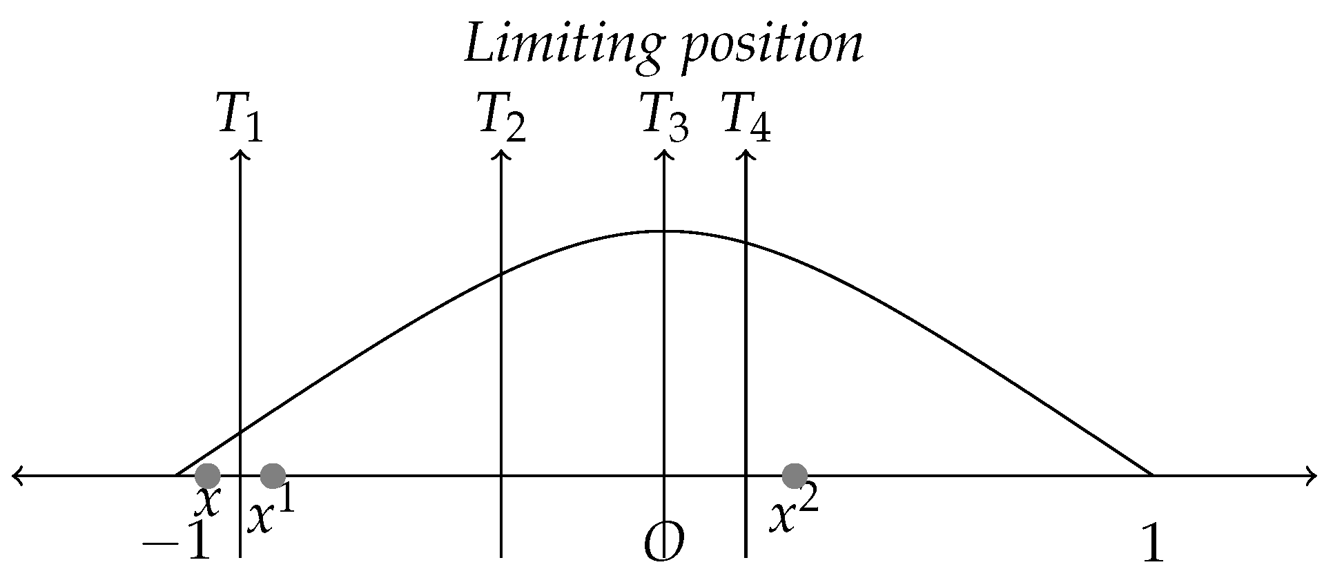
We first consider one simple example on a bounded domain in one-dimensional Euclidean space ${\mathbb{R}}^1$. Assume that u is a positive solution of an equation defined in a symmetric domain $\mathrm{\Omega }$ and it equals 0 on the boundary. In addition, the equation is symmetric with respect to $\mathrm{\Omega }$; one can refer to Figure 1 for a visual representation.

Figure 1. Method of moving planes in one dimension.

Let $\mathrm{\Omega }=(-1,1)$ and $u(-1)=0=u\left(1\right)$. In one dimension, the moving plane reduces to a point:

$$\begin{array}{c}\hfill T_{\lambda }=\left\{x\right|x=\lambda \}.\end{array}$$

Let

$$\begin{array}{c}\hfill {\mathrm{\Sigma }}_{\lambda }=\left\{x\right|-1<x<\lambda \}\end{array}$$

be the region to the left of $T_{\lambda }$ in $\mathrm{\Omega }$, and

$$\begin{array}{c}\hfill x^{\lambda }=2\lambda -x\end{array}$$

be the reflection of x about $T_{\lambda }$.

We compare $u\left(x^{\lambda }\right)$ and $u\left(x\right)$. For simplicity, set $w_{\lambda }=u\left(x^{\lambda }\right)-u\left(x\right)$. We may expect that when $T_{\lambda }$ is sufficiently close to $-1$, we have

$$\begin{array}{c}\hfill w_{\lambda }\ge 0,\forall x\in {\mathrm{\Sigma }}_{\lambda }.\end{array}$$

(6)

Then, we move the plane T continuously to the right as long as inequality (6) holds until its limiting position and prove that u must be symmetric about the limiting plane. From the Figure 1, when the plane T is moved to the $T_2$ position, inequality (6) is still valid; hence, we can keep moving it. The $T_3$ position is the limiting one, because after passing it, say at the $T_4$ position, (6) is violated.

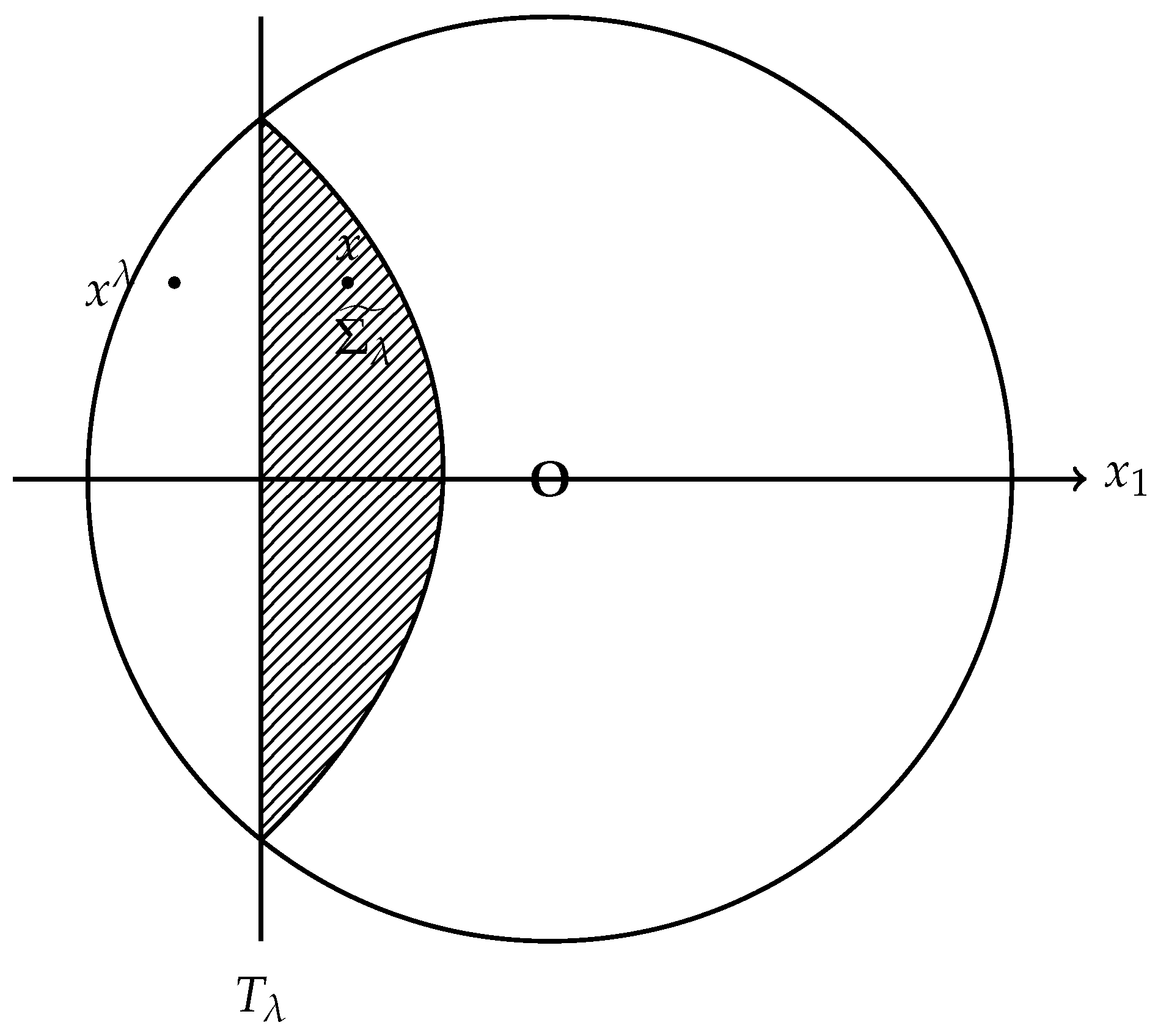
We can generalize this method to higher-dimensional symmetric domain, say $B_1\left(0\right)$. Given an arbitrary real number $\lambda ,$ let

$$\begin{array}{c}\hfill T_{\lambda }=\{x\in {\mathbb{R}}^n\mid x_1=\lambda \mathrm{for}\mathrm{some}\lambda \in \mathbb{R}\}\end{array}$$

be the defined moving planes, and

$$\begin{array}{c}\hfill {\mathrm{\Sigma }}_{\lambda }=\{x\in {\mathbb{R}}^n\mid x_1<\lambda \}\end{array}$$

be the domain situated to the left of the plane, and

$$\begin{array}{c}\hfill x^{\lambda }=(2\lambda -x_1,x_2,...,x_n)\end{array}$$

be the result of reflecting x over the plane $T_{\lambda }.$

$$\begin{array}{c}\hfill \widetilde{{\mathrm{\Sigma }}_{\lambda }}=\{x\mid x^{\lambda }\in {\mathrm{\Sigma }}_{\lambda }\}\end{array}$$

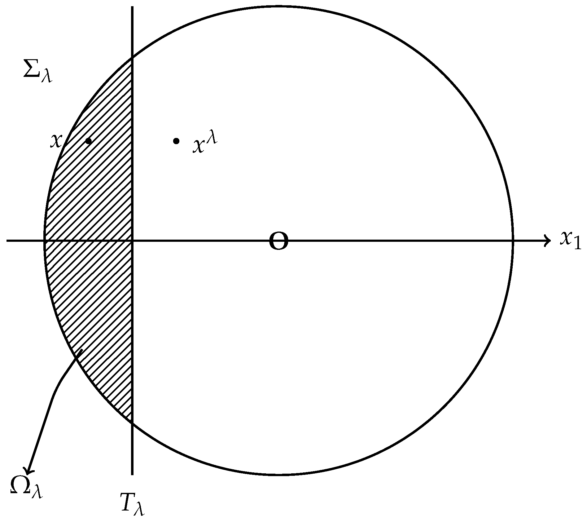
is the reflection of ${\mathrm{\Sigma }}_{\lambda }$ about the plane $T_{\lambda }$; see Figure 2. Since in our research $u(x,t)=0$ outside $B_1\left(0\right)$, therefore, $\widetilde{{\mathrm{\Sigma }}_{\lambda }}$ only reflects the intersection part of $B_1\left(0\right)$ and ${\mathrm{\Sigma }}_{\lambda }$, and

$$\begin{array}{c}\hfill {\mathrm{\Omega }}_{\lambda }={\mathrm{\Sigma }}_{\lambda }\cap B_1\left(0\right)\end{array}$$

be the intersection of $B_1\left(0\right)$ and ${\mathrm{\Sigma }}_{\lambda }$. One can refer to Figure 3 for a visual representation.

Figure 2. Reflection about the moving plane.

Figure 3. ${\mathrm{\Sigma }}_{\lambda }$ and ${\mathrm{\Omega }}_{\lambda }$.

Let $u(x,t)$ and $v(x,t)$ be positive solutions to Equation (2). We conduct a comparison between the values of $u(x,t)$ and those of $u_{\lambda }(x,t)$, where $u_{\lambda }(x,t)$ is defined as $u(x^{\lambda },t)$. Similarly, we perform a comparison of the values of $v(x,t)$ with those of $v_{\lambda }(x,t)$, with $v_{\lambda }(x,t)$ being equal to $v(x^{\lambda },t)$; let

$$\begin{array}{c}\hfill U_{\lambda }(x,t)=u_{\lambda }(x,t)-u(x,t).\end{array}$$

$$\begin{array}{c}\hfill V_{\lambda }(x,t)=v_{\lambda }(x,t)-v(x,t).\end{array}$$

The core aspect of the proof lies in demonstrating that

$$\begin{array}{c}\hfill U_{\lambda }(x,t)\ge 0,V_{\lambda }(x,t)\ge 0,(x,t)\in {\mathrm{\Omega }}_{\lambda }\times \mathbb{R}.\end{array}$$

(7)

This establishes an initial condition for initiating the movement of the plane. Subsequently, in the second phase, we displace the plane towards the right, continuing this process as long as inequality (7) remains valid, until it reaches its limiting position. This is performed to demonstrate that the functions u and v exhibit symmetry with respect to the limiting plane. Typically, the narrow region principle is employed to establish the validity of inequality (7), given that $U_{\lambda }$ and $V_{\lambda }$ are characterized as anti-symmetric functions:

$$\begin{array}{c}\hfill U_{\lambda }(x,t)=-U_{\lambda }(x^{\lambda },t),\end{array}$$

$$\begin{array}{c}\hfill V_{\lambda }(x,t)=-V_{\lambda }(x^{\lambda },t).\end{array}$$

In high-dimensional spaces, if we only aim to prove properties of solutions in specific directions, any symmetric domain can be used, as long as the equation is symmetric with respect to this domain. For example, this applies to the semi-major axis, semi-intermediate axis, and semi-minor axis of an ellipsoid. However, if we need to prove the radial symmetry of solutions in any arbitrary direction $x_i$, then a unit ball must be used.

4. Regularity and Maximal Regularity of Solutions of Fractional Parabolic Systems

We rely on the following theorem of Liu (2025) [7] to establish the existence of solutions of parabolic fractional equations.

Theorem 3 

(Liu, 2025, p. 3 [7]). Let $B_1\left(0\right)$ be a unit ball. Let $0<s<1$, assuming that $u(x,t)\in \left(C_{loc}^{1,1}\left(B_1\left(0\right)\right)\cap C\left(\overline{B_1\left(0\right)}\right)\right)\times \mathbb{R}$ is a positive bounded classical solution of

$$\begin{array}{c}\hfill \left\{\begin{array}{cc}{\displaystyle \frac{\partial u}{\partial t}}(x,t)+{(-\Delta )}^{s}u(x,t)=f(t,|x|,u),\hfill & (x,t)\in B_1\left(0\right)\times \mathbb{R},\hfill \\ u(x,t)\equiv 0,\hfill & x\ne B_1\left(0\right),\hfill \end{array}\right.\end{array}$$

(8)

where f is Lipschitz continuous; then, the solution of (8) satisfies the $L_p$-$L_q$ maximal regularity estimate:

$$\begin{array}{c}\hfill \parallel e^{-\gamma t}{u}_t{\parallel }_{L_p(\mathbb{R},L_q\left(B_1\left(0\right)\right))}+\parallel e^{-\gamma t}{\nabla }^2{u\parallel }_{L_p(\mathbb{R},L_q\left(B_1\left(0\right)\right))}\le C{\parallel e^{-\gamma t}f\parallel }_{L_p(\mathbb{R},L_q\left(B_1\left(0\right)\right))}\end{array}$$

(9)

for any $\gamma \ge 0$. Since $f\in C_0^{\infty }({\mathbb{R}}_{+}^n\times \mathbb{R})$, and $C_0^{\infty }({\mathbb{R}}_{+}^n\times \mathbb{R})$ is dense in $L_{p,0}({\mathbb{R}}_{+},L_q\left({\mathbb{R}}^n\right))$.

In (9), $L_p(\mathbb{R},L_q\left(B_1\left(0\right)\right))$ consists of functions $u:\mathbb{R}\to L^q\left(B_1\left(0\right)\right)$, such that the following norm is finite:

$$\begin{array}{c}\hfill {\parallel u\parallel }_{L_p(\mathbb{R},L_q\left(B_1\left(0\right)\right))}={\left({\int }_{\mathbb{R}}{\parallel u\left(t\right)\parallel }_{L_q}^{p}dt\right)}^{{\displaystyle \frac{1}{q}}}<\infty \end{array}$$

which does not assume time-weighted norms as shown in [21]. The exponential stability result is derived from the analyticity of the semigroup, not from explicit weighting.

We can generalize Theorem 3 if $f=f\left(v\right)$ is only Hölder continuous. A function $f:{\mathbb{R}}^n\to \mathbb{R}$ is Hölder continuous if there exist constants $C>0$ and $\alpha \in (0,1]$, such that for all $x,y\in {\mathbb{R}}^n$

$$\begin{array}{c}\hfill |f\left(v_1\right)-f\left(v_2\right)|\le |v_1-v_2{|}^{\alpha }.\end{array}$$

A larger $\alpha$ implies stronger continuity for f. $H^s\left({\mathbb{R}}^n\right)$ is a Sobolev space where s can be a non-integer. For $s>{\displaystyle \frac{n}{2}}$, the Sobolev embedding theorem states that $H^s$ can be continuously embedded into Hölder continuous function spaces.

Theorem 4 

(Sobolev embedding theorem). If $s>{\displaystyle \frac{n}{2}}$, then $H^s\left({\mathbb{R}}^n\right)$ embeds continuously into $C^{k,\alpha }\left({\mathbb{R}}^n\right)$, where k is the largest integer satisfying $k<s-{\displaystyle \frac{n}{2}}$, $\alpha =s-{\displaystyle \frac{n}{2}}-k\in (0,1]$. $C^{k,\alpha }$ denotes the space of functions that are k-times continuously differentiable, with k-th derivatives being α-Hölder continuous. If s is not an integer and $s-{\displaystyle \frac{n}{2}}\in (0,1]$, then $H^s$ embeds into $C^{0,\alpha }\left({\mathbb{R}}^n\right)$, where $\alpha =s-{\displaystyle \frac{n}{2}}$.

The solution u in the maximal regularity (9) often belongs to a space like

$$\begin{array}{c}\hfill u\in W_p^{2,1}(\mathbb{R},L_q\left(B_1\left(0\right)\right))\cap L_p(\mathbb{R},W^{2,q}\left(B_1\left(0\right)\right)),\end{array}$$

which is a Sobolev-type space with mixed derivatives. For f to be in $L_p(\mathbb{R},L_q\left(B_1\left(0\right)\right))$, we do not necessarily need Hölder continuity in time, but we consider f to be Hölder continuous in space. Specifically, if $f\in C^{0,\alpha }\left(B_1\left(0\right)\right)$, then f can be embedded into $W^{s,q}\left(B_1\left(0\right)\right)$ for $s<\alpha +{\displaystyle \frac{n}{p}}$, where n is the spatial dimension, provided that $s>{\displaystyle \frac{n}{q}}$ for the embedding into Hölder spaces is held. Our goal is to show that f being Hölder continuous implies that u is in $H^s$, and then use embedding to control u in $L_q$. To prove that u belongs to $H^s$ when f is Hölder continuous, we would typically use the fact that the heat equation with Hölder continuous f has a solution u that is smooth in time and space by parabolic regularity theory (see this part in [22]). Then, u satisfies the maximal regularity estimate in terms of $H^s$-type norms.

Then, we use the Hölder continuity of f to bound the $H^s$-norm of u in terms of the Hölder norm of f. Here is a sketch of how to bound ${\parallel u\parallel }_{H^s}$:

First, we multiply $u_t-\Delta u=f$ by u and integrate over $B_1\left(0\right)$:

$$\begin{array}{c}\hfill {\displaystyle \frac{1}{2}}{\displaystyle \frac{d}{dt}}{\parallel u\parallel }_{L_2}^2+{\parallel \nabla u\parallel }_{L_2}^2={\int }_{B_1\left(0\right)}fudx,\end{array}$$

then,

$$\begin{array}{c}\hfill \left|{\int }_{B_1\left(0\right)}fudx\right|\le {\parallel f\parallel }_{L_{\infty }}{\parallel u\parallel }_{L_1}\le {\parallel f\parallel }_{L_{\infty }}{\parallel u\parallel }_{L_2}.\end{array}$$

This gives a basic energy estimate for ${\parallel u\parallel }_{L_2}$.

For higher-order derivatives, we differentiate the PDE with respect to x to get estimates on $\nabla u$, ${\nabla }^{2}u$, …, and use energy estimates for $\nabla u$ to bound ${\parallel \nabla u\parallel }_{L_2}$, and similarly for higher derivatives. Then, we use interpolation inequalities to relate ${\parallel u\parallel }_{H^s}$ to lower-order norms; for example, if s is an integer, then

$$\begin{array}{c}\hfill {\parallel u\parallel }_{H^s}\le C\left({\parallel u\parallel }_{L_2}+\sum _{\left|\beta \right|=s}{\parallel {\partial }^{\beta }u\parallel }_{L_2}\right).\end{array}$$

We bound each term using the energy estimates and the Hölder continuity of f. For non-integer s, we use fractional Sobolev norms and interpolation (e.g., the Gagliardo–Nirenberg inequality).

Combining these steps, we can derive a bound of the form:

$$\begin{array}{c}\hfill {\parallel u\parallel }_{H^s}\le C{\parallel f\parallel }_{C^{0,\alpha }}\end{array}$$

where C depends on $s,\alpha$, and the domain $B_1\left(0\right)$. The exact value of s depends on the regularity of f and the parabolic operator. For $f\in C^{0,\alpha }$, we can typically bound u in $H^s$ for s up to $2+\alpha$.

When considering the case where $\alpha ,\beta \in (0,2)$ are different and $a\to 0_{+}$, the original assumptions $\left(M1\right)$ and $\left(M2\right)$ on f and g (non-decreasing property and uniform Lipschitz continuity) are still fundamental for guaranteeing the symmetry of the solutions u and v with respect to the origin. The fractional Laplacian ${(-\Delta )}^{{\displaystyle \frac{\alpha }{2}}}$ has the following Fourier transform representation:

$$\begin{array}{c}\hfill F({(-\Delta )}^{{\displaystyle \frac{\alpha }{2}}}u)\left(\xi \right)={\left|\xi \right|}^{\alpha }F\left(u\right)\left(\xi \right),\end{array}$$

where F is the Fourier transform. As $\alpha \to 0_{+}$, ${\left|\xi \right|}^{\alpha }\to 1$ for all $\xi \in {\mathbb{R}}^n$. So, the equation

$$\begin{array}{c}\hfill {\displaystyle \frac{\partial u}{\partial t}}+{(-\Delta )}^{{\displaystyle \frac{\alpha }{2}}}u(x,t)=f\left(v(x,t)\right)\end{array}$$

approaches

$$\begin{array}{c}\hfill {\displaystyle \frac{\partial u}{\partial t}}+u(x,t)=f\left(v(x,t)\right)\end{array}$$

as $a\to 0_{+}$. Then, we have the following system:

$$\begin{array}{c}\hfill \left\{\begin{array}{c}{\displaystyle \frac{\partial u}{\partial t}}+u(x,t)=f\left(v(x,t)\right),\hfill \\ {\displaystyle \frac{\partial v}{\partial t}}+{(-\Delta )}^{{\displaystyle \frac{\beta }{2}}}v(x,t)=g\left(u(x,t)\right),\hfill \end{array}\right.\end{array}$$

(10)

with certain initial conditions and homogeneous boundary conditions. Now, we would like to show the regularity of the system (10).

4.1. Weak Formulation

Let $\phi \in C_c^{\infty }(B_1\left(0\right)\times (0,T))$. Multiply the first equation ${\displaystyle \frac{\partial u}{\partial t}}+u(x,t)=f\left(v(x,t)\right)$ by $\phi$ and integrate over $\mathrm{\Omega }\times (0,t)$ for $t\in (0,T]$:

$$\begin{array}{c}\hfill {\int }_0^t{\int }_{B_1\left(0\right)}{\displaystyle \frac{\partial u}{\partial s}}\phi dxds+{\int }_0^t{\int }_{B_1\left(0\right)}u\phi dxds={\int }_0^t{\int }_{B_1\left(0\right)}f\left(v\right)\phi dxds,\end{array}$$

using integration by parts with respect to s, we derive

$$\begin{array}{c}{\int }_{B_1\left(0\right)}u(x,t)\phi (x,t)dx-{\int }_{B_1\left(0\right)}u(x,0)\phi (x,0)dx-{\int }_0^t{\int }_{B_1\left(0\right)}u{\displaystyle \frac{\partial \phi }{\partial s}}dxds\hfill \\ \hspace{1em}\hspace{1em}\hspace{1em}\hspace{1em}\hspace{1em}\hspace{1em}\hspace{1em}\hspace{1em}\hspace{1em}\hspace{1em}\hspace{1em}\hspace{1em}\hspace{1em}\hspace{1em}\hspace{1em}\hspace{1em}+{\int }_0^t{\int }_{B_1\left(0\right)}u\phi dxds={\int }_0^t{\int }_{B_1\left(0\right)}f\left(v\right)\phi dxds.\hfill \end{array}$$

For a test function $\psi \in C_c^{\infty }(B_1\left(0\right)\times (0,T))$, we multiply the second equation ${\displaystyle \frac{\partial v}{\partial t}}+{(-\Delta )}^{{\displaystyle \frac{\beta }{2}}}v(x,t)=g\left(u(x,t)\right)$ by $\psi$ and integrate over ${\mathbb{R}}^n\times (0,t)$, using the fact that $v=0$ outside $B_1\left(0\right)$:

$$\begin{array}{c}\hfill {\int }_0^t{\int }_{{\mathbb{R}}^n}{\displaystyle \frac{\partial v}{\partial s}}\psi dxds+{\int }_0^t{\int }_{{\mathbb{R}}^n}{(-\Delta )}^{{\displaystyle \frac{\beta }{2}}}v\phi dxds={\int }_0^t{\int }_{{\mathbb{R}}^n}g\left(u\right)\psi dxds.\end{array}$$

By integration by parts with respect to s and using the properties of the fractional Laplacian: ${\int }_{{\mathbb{R}}^n}{(-\Delta )}^{{\displaystyle \frac{\beta }{2}}}v\psi dx={\int }_{{\mathbb{R}}^n}v{(-\Delta )}^{{\displaystyle \frac{\beta }{2}}}\psi dx$ for appropriate functions v and $\psi$ (see the proof of this equation in [23]), we have

$$\begin{array}{c}{\int }_{{\mathbb{R}}^n}v(x,t)\psi (x,t)dx-{\int }_{{\mathbb{R}}^n}v(x,0)\psi (x,0)dx-{\int }_0^t{\int }_{{\mathbb{R}}^n}v{\displaystyle \frac{\partial \psi }{\partial s}}dxds\hfill \\ \hspace{1em}\hspace{1em}\hspace{1em}\hspace{1em}\hspace{1em}\hspace{1em}\hspace{1em}\hspace{1em}\hspace{1em}\hspace{1em}\hspace{1em}\hspace{1em}\hspace{1em}\hspace{1em}\hspace{1em}+{\int }_0^t{\int }_{{\mathbb{R}}^n}v{(-\Delta )}^{{\displaystyle \frac{\beta }{2}}}\psi dxds={\int }_0^t{\int }_{{\mathbb{R}}^n}g\left(u\right)\psi dxds.\hfill \end{array}$$

4.2. Energy Estimates

Multiply the first equation ${\displaystyle \frac{\partial u}{\partial t}}+u(x,t)=f\left(v(x,t)\right)$ by u and integrate over $B_1\left(0\right)$:

$$\begin{array}{c}\hfill {\int }_{B_1\left(0\right)}{\displaystyle \frac{\partial u}{\partial t}}udx+{\int }_{B_1\left(0\right)}{u}^{2}dx={\int }_{B_1\left(0\right)}f\left(v\right)udx,\end{array}$$

we derive

$$\begin{array}{c}\hfill {\displaystyle \frac{1}{2}}{\displaystyle \frac{d}{dt}}{\int }_{B_1\left(0\right)}{u}^{2}dx+{\int }_{B_1\left(0\right)}{u}^{2}dx={\int }_{B_1\left(0\right)}f\left(v\right)udx.\end{array}$$

Through the Cauchy–Schwarz inequality and Young’s inequality, since ${\left|f\left(v\right)\right|}^2\le {C(1+|v|}^2)$ because f is Lipschitz continuous, we have

$$\begin{array}{c}\hfill {\displaystyle \frac{1}{2}}{\displaystyle \frac{d}{dt}}{\int }_{B_1\left(0\right)}{u}^{2}dx+(1-{\displaystyle \frac{ϵ}{2}}){\int }_{B_1\left(0\right)}{u}^{2}dx\le {\displaystyle \frac{2C}{ϵ}}{\int }_{B_1\left(0\right)}{(1+|v|}^2)dx+{\displaystyle \frac{ϵ}{2}}{\int }_{B_1\left(0\right)}{u}^{2}dx,\end{array}$$

Let $ϵ=1$, then

$$\begin{array}{c}\hfill {\displaystyle \frac{d}{dt}}{\int }_{B_1\left(0\right)}{u}^{2}dx+{\int }_{B_1\left(0\right)}{u}^{2}dx\le C(1+{\int }_{B_1\left(0\right)}{v}^{2}dx).\end{array}$$

Multiply the second equation ${\displaystyle \frac{\partial v}{\partial t}}+{(-\Delta )}^{{\displaystyle \frac{\beta }{2}}}v(x,t)=g\left(u(x,t)\right)$ by v and integrate over ${\mathbb{R}}^n$:

$$\begin{array}{c}\hfill {\int }_{{\mathbb{R}}^n}{\displaystyle \frac{\partial v}{\partial t}}vdx+{\int }_{{\mathbb{R}}^n}v{(-\Delta )}^{{\displaystyle \frac{\beta }{2}}}vdx={\int }_{{\mathbb{R}}^n}g\left(u\right)vdx,\end{array}$$

through the non-negativity of the fractional Dirichlet form and Lipschitz continuity of g, we derive

$$\begin{array}{c}\hfill {\displaystyle \frac{1}{2}}{\displaystyle \frac{d}{dt}}{\int }_{{\mathbb{R}}^n}{v}^{2}dx\le {\displaystyle \frac{C}{2}}{\int }_{{\mathbb{R}}^n}(1+u^2)dx\end{array}$$

$$\begin{array}{c}\hfill {\displaystyle \frac{d}{dt}}{\int }_{{\mathbb{R}}^n}{v}^{2}dx\le C(1+{\int }_{{\mathbb{R}}^n}{u}^{2}dx).\end{array}$$

Let $E_1\left(t\right)={\int }_{B_1\left(0\right)}{u}^{2}dx$ and $E_2\left(t\right)={\int }_{{\mathbb{R}}^2}{v}^{2}dx$; summing the two inequalities, we have

$$\begin{array}{c}\hfill {\displaystyle \frac{d}{dt}}(E_1\left(t\right)+E_2\left(t\right))+\left(E_1\left(t\right)\right)\le C(1+E_1\left(t\right)+E_2\left(t\right)),\end{array}$$

Let $E\left(t\right)=E_1\left(t\right)+E_2\left(t\right)$. Then

$$\begin{array}{c}\hfill {\displaystyle \frac{dE}{dt}}\le C(1+E),\end{array}$$

by Gronwall’s inequality, if $E\left(0\right)={\int }_{B_1\left(0\right)}{u}_0^{2}dx+{\int }_{{\mathbb{R}}^n}{v}_0^{2}dx$, then $E\left(t\right)\le (E\left(0\right)+Ct)e^{Ct}$. This shows that $u\in L_{\infty }(0,T;L_2\left(B_1\left(0\right)\right))$ and $v\in L_{\infty }(0,T;L_2\left({\mathbb{R}}^n\right))$.

4.3. Higher-Order Regularity

Differentiate the first equation with respect to t:

$$\begin{array}{c}\hfill {\displaystyle \frac{{\partial }^{2}u}{\partial t^2}}+{\displaystyle \frac{\partial u}{\partial t}}=f^{\prime }\left(v\right){\displaystyle \frac{\partial v}{\partial t}},\end{array}$$

multiply this equation by ${\displaystyle \frac{\partial u}{\partial t}}$ and integrate over $\mathrm{\Omega }$. Using the Cauchy–Schwarz inequality, the fact that $u\in L_{\infty }(0,T;L_2\left(B_1\left(0\right)\right))$ and the Lipschitz continuity of $f^{\prime }$, we have ${\displaystyle \frac{\partial u}{\partial t}}\in L_{\infty }(0,T;L_2\left(B_1\left(0\right)\right))$. Since ${\displaystyle \frac{\partial u}{\partial t}}+u=f\left(v\right)$ and $u,{\displaystyle \frac{\partial u}{\partial t}}\in L_{\infty }(0,T;L_2\left(B_1\left(0\right)\right))$, and also $f\left(v\right)\in L_{\infty }(0,T;L_2\left(B_1\left(0\right)\right))$, we can use elliptic-type estimates (in the time-dependent sense) to show $u\in H^1(0,T;L_2\left(\mathrm{\Omega }\right))\cap L_{\infty }(0,T;L_2\left(B_1\left(0\right)\right))$. Differentiate the second equation with respect to t:

$$\begin{array}{c}\hfill {\displaystyle \frac{{\partial }^{2}v}{\partial t^2}}+{(-\Delta )}^{{\displaystyle \frac{\beta }{2}}}{\displaystyle \frac{\partial v}{\partial t}}=g^{\prime }\left(u\right){\displaystyle \frac{\partial u}{\partial t}},\end{array}$$

multiply this equation by ${\displaystyle \frac{\partial v}{\partial t}}$ and integrate over ${\mathbb{R}}^n$. Using the properties of the fractional Laplacian, the Cauchy–Schwarz inequality, and the Lipschitz continuity of $g^{\prime }$, we can show that ${\displaystyle \frac{\partial v}{\partial t}}\in L_{\infty }(0,T;L_2\left({\mathbb{R}}^n\right))$. By using the fact that ${\displaystyle \frac{\partial v}{\partial t}}+{(-\Delta )}^{{\displaystyle \frac{\beta }{2}}}v=g\left(u\right)$ and the regularity results for the fractional heat equation, we can show that $v\in H^1(0,T;L_2\left({\mathbb{R}}^n\right))\cap L_{\infty }(0,T;H^{{\displaystyle \frac{\beta }{2}}}\left({\mathbb{R}}^n\right))$. In conclusion, for the initial values $u_0\in L_2\left(B_1\left(0\right)\right)$ and $v_0\in L_2\left({\mathbb{R}}^n\right)$, and if $f,g$ are Lipschitz continuous, then the weak solution $(u,v)$ of the parabolic system satisfies

$$\begin{array}{c}\hfill u\in H^1(0,T;L_2\left(B_1\left(0\right)\right))\cap L_{\infty }(0,T;L^2\left(\mathrm{\Omega }\right))\end{array}$$

and

$$\begin{array}{c}\hfill v\in H^1(0,T;L_2\left({\mathbb{R}}^n\right))\cap L_{\infty }(0,T;H^{{\displaystyle \frac{\beta }{2}}}\left({\mathbb{R}}^n\right)).\end{array}$$

Also, the minimal regularity conditions on $f,g$ should be

$$\begin{array}{c}\hfill f\left(v\right)\in L_{\infty }(0,T;L_2\left(B_1\left(0\right)\right))\end{array}$$

and

$$\begin{array}{c}\hfill g\left(u\right)\in L_{\infty }(0,T;H^{{\displaystyle \frac{\beta }{2}}}\left({\mathbb{R}}^n\right)).\end{array}$$

In the reference [18], Liu (2024) offered a succinct elucidation of the foundational logic and principles that underpin the existence of maximal regularity for both parabolic and hyperbolic differential equations. By relying on this source, we can conclude that a necessary condition for the existence of maximal regularity in parabolic differential equations is that the eigenvalues of the operator corresponding to the spatial variables must be strictly less than 1. In the expression (9), we note that as $\gamma$ approaches infinity and $t>0$, the norm $\parallel e^{-\gamma t}{\nabla }^2{u\parallel }_{L_p(\mathbb{R},L_q\left({\mathbb{R}}^n\right)}$ can be bounded above by 1. Nevertheless, when $\gamma$ is not large enough or $t<0$, in order to guarantee that the eigenvalues of the nonlocal fractional Laplacian operator stay below 1, we enforce the requirement $u(x,t)\stackrel{\mathrm{a}.\mathrm{e}.}{\to }{u}_0(x,t),v(x,t)\stackrel{\mathrm{a}.\mathrm{e}.}{\to }{v}_0(x,t),(x,t)\in B_1\left(0\right)\times \mathbb{R}$ as shown in Theorem 1. Convergence condition is used to regulate the growth of ${(-\Delta )}^{s}u(x,t)$ and ${(-\Delta )}^{s}v(x,t)$.

5. Narrow Region Principle in Systems of Parabolic Laplacian Equations

We present a detailed proof for Theorem 2. Subsequently, in the following sections, we leverage Theorem 2 to contribute a comprehensive proof for Theorem 1.

In the event that Equation $\left(4\right)$ fails to be valid, then the lower semi-continuity of $U(x,t)$ on $\overline{\mathrm{\Omega }}\times [\underline{t},T]$ guarantees that there is at least one $(x^o,t^o)\in \overline{\mathrm{\Omega }}\times (\underline{t},T]$, such that

$$\begin{array}{c}\hfill U(x^o,t^o)=\underset{\overline{\mathrm{\Omega }}\times (\underline{t},T]}{\min }U<0.\end{array}$$

Given that $(x^o,t^o)$ serves as the minimum point, it follows that

$$\begin{array}{c}\hfill {\displaystyle \frac{\partial U(x^o,t^o)}{\partial t}}=0.\end{array}$$

(11)

Moreover, by further analyzing condition (3), it can be inferred that the point $(x^o,t^o)$ lies within the interior of $\overline{\mathrm{\Omega }}\times [\underline{t},T]$. Subsequently, we proceed as follows

$$\begin{array}{cc} & {(-\Delta )}^{{\displaystyle \frac{\alpha }{2}}}U(x^o,t^o)\hfill \\ =& C_{n,\alpha }P.V.{\int }_{{\mathbb{R}}^n}{\displaystyle \frac{U(x^o,t^o)-U(y,t^o)}{|x^o{-y|}^{n+\alpha }}}dy\hfill \\ =& C_{n,\alpha }P.V.\left\{{\int }_{\mathrm{\Sigma }}{\displaystyle \frac{U(x^o,t^o)-U(y,t^o)}{|x^o{-y|}^{n+\alpha }}}dy+{\int }_{\tilde{\mathrm{\Sigma }}}{\displaystyle \frac{U(x^o,t^o)-U(y,t^o)}{|x^o{-y|}^{n+\alpha }}}dy\right\}\hfill \\ =& C_{n,\alpha }P.V.\left\{{\int }_{\mathrm{\Sigma }}{\displaystyle \frac{U(x^o,t^o)-U(y,t^o)}{|x^o{-y|}^{n+\alpha }}}dy+{\int }_{\mathrm{\Sigma }}{\displaystyle \frac{U(x^o,t^o)-U(y^{\lambda },t^o)}{|x^o-y^{\lambda }{|}^{n+\alpha }}}dy\right\}\hfill \\ =& C_{n,\alpha }P.V.\left\{{\int }_{\mathrm{\Sigma }}{\displaystyle \frac{U(x^o,t^o)-U(y,t^o)}{|x^o{-y|}^{n+\alpha }}}dy+{\int }_{\mathrm{\Sigma }}{\displaystyle \frac{U(x^o,t^o)+U(y,t^o)}{|x^o-y^{\lambda }{|}^{n+\alpha }}}dy\right\}\hfill \\ \le & C_{n,\alpha }\left\{{\int }_{\mathrm{\Sigma }}{\displaystyle \frac{U(x^o,t^o)-U(y,t^o)}{|x^o-y^{\lambda }{|}^{n+\alpha }}}dy+{\displaystyle \frac{U(x^o,t^o)+U(y,t^o)}{|x^o-y^{\lambda }{|}^{n+\alpha }}}dy\right\}\hfill \\ =& C_{n,\alpha }{\int }_{\mathrm{\Sigma }}{\displaystyle \frac{2U(x^o,t^o)}{|x^o-y^{\lambda }{|}^{n+\alpha }}}\hfill \\ \le & {\displaystyle \frac{cU(x^o,t^o)}{d^{\alpha }}}\hfill \\ <& 0,\hfill \end{array}$$

(12)

where d denotes the distance function. If

$$\begin{array}{c}\hfill t^o<T,\end{array}$$

$$\begin{array}{c}\hfill {\displaystyle \frac{\partial U}{\partial t}}(x^o,t^o)=0.\end{array}$$

(13)

If

$$\begin{array}{c}\hfill t^o=T,\end{array}$$

$$\begin{array}{c}\hfill {\displaystyle \frac{\partial U}{\partial t}}(x^o,t^o)\le 0.\end{array}$$

(14)

Combining (3), (12), (13) and (14), we deduce

$$\begin{array}{c}\hfill c_{1}V(x^o,t^o)\le {\displaystyle \frac{\partial U(x^o,t^o)}{\partial t}}+{(-\Delta )}^{{\displaystyle \frac{\alpha }{2}}}U(x^o,t^o)\le {\displaystyle \frac{cU(x^o,t^o)}{d^{\alpha }}}<0.\end{array}$$

(15)

Therefore, we have

$$\begin{array}{c}\hfill V(x^o,t^o)<0.\end{array}$$

This indicates that there is at least one pair $(\overline{x},\overline{t})$ belonging to $\overline{\mathrm{\Omega }}\times (\underline{t},T]$, satisfying

$$\begin{array}{c}\hfill V(\overline{x},\overline{t})=\underset{\overline{\mathrm{\Omega }}\times (\underline{t},T]}{\min }V<0,\end{array}$$

The point $(\overline{x},\overline{t})$ is defined as the minimum point of the function V over the domain $\overline{\mathrm{\Omega }}\times (\underline{t},T]$. This means that for all $(x,t)\in \overline{\mathrm{\Omega }}\times (\underline{t},T]$, we have $V(x,t)\ge V(\overline{x},\overline{t})$. In the context of calculus of variations or optimization, a necessary condition for a function to attain a local minimum at a point is that the first-order partial derivatives of the function with respect to its variables vanish at that point. This is a fundamental result from the theory of critical points and can be derived from the Taylor series expansion of the function around the minimum point. Applying this necessary condition to our function V, we conclude that the partial derivatives of V with respect to x and t must be zero at $(\overline{x},\overline{t})$, so that

$$\begin{array}{c}\hfill {\displaystyle \frac{\partial V}{\partial t}}(x,t){|}_{(\overline{x},\overline{t})}=0,\end{array}$$

(16)

for convenience, we denote

$$\begin{array}{c}\hfill {\displaystyle \frac{\partial V}{\partial t}}(\overline{x},\overline{t})={\displaystyle \frac{\partial V}{\partial t}}(x,t){|}_{(\overline{x},\overline{t})}=0,\end{array}$$

following the same argument with (12), we are able to infer that

$$\begin{array}{c}\hfill {(-\Delta )}^{{\displaystyle \frac{\beta }{2}}}V(\overline{x},\overline{t})\le {\displaystyle \frac{cV(\overline{x},\overline{t})}{d^{\beta }}}<0.\end{array}$$

From (15), we derive

$$\begin{array}{c}\hfill c_{1}V(x^o,t^o){\displaystyle \frac{d^{\alpha }}{c}}\le U(x^o,t^o).\end{array}$$

Combine (3) and (16), we have

$$\begin{array}{cc} & {\displaystyle \frac{\partial V}{\partial t}}(\overline{x},\overline{t})+{(-\Delta )}^{{\displaystyle \frac{\beta }{2}}}V(\overline{x},\overline{t})-c_{2}U(\overline{x},\overline{t})\hfill \\ :=& {(-\Delta )}^{{\displaystyle \frac{\beta }{2}}}V(\overline{x},\overline{t})-c_{2}U(\overline{x},\overline{t})\ge 0,\hfill \end{array}$$

we derive

$$\begin{array}{ccc}0\hfill & \le & {(-\Delta )}^{{\displaystyle \frac{\beta }{2}}}V(\overline{x},\overline{t})-c_{2}U(\overline{x},\overline{t})\hfill \\ & \le & {\displaystyle \frac{cV(\overline{x},\overline{t})}{d^{\beta }}}-c_{2}U(\overline{x},\overline{t})\hfill \\ & \le & {\displaystyle \frac{cV(\overline{x},\overline{t})}{d^{\beta }}}-c_{2}U(x^o,t^o)\hfill \\ & \le & {\displaystyle \frac{cV(\overline{x},\overline{t})}{d^{\beta }}}-c_2(c_{1}V(x^o,t^o){\displaystyle \frac{d^{\alpha }}{c}})\hfill \\ & \le & {\displaystyle \frac{cV(\overline{x},\overline{t})}{d^{\beta }}}-c_2(c_{1}V(\overline{x},\overline{t}){\displaystyle \frac{d^{\alpha }}{c}})\hfill \\ & \le & {\displaystyle \frac{cV(\overline{x},\overline{t})}{d^{\beta }}}(1-c_2{c}_1{\displaystyle \frac{d^{\alpha +\beta }}{c^2}}).\hfill \end{array}$$

(17)

Provided that $\lambda$ is in a sufficiently small neighborhood of $-1$, d would be remarkably small,

$$\begin{array}{c}\hfill c_2{c}_1{\displaystyle \frac{d^{\alpha +\beta }}{c^2}}<<1,\end{array}$$

and

$$\begin{array}{c}\hfill V(\overline{x},\overline{t})<0,\end{array}$$

so we derive

$$\begin{array}{c}\hfill {\displaystyle \frac{cV(\overline{x},\overline{t})}{d^{\beta }}}(1-c_2{c}_1{\displaystyle \frac{d^{\alpha +\beta }}{c^2}})<0.\end{array}$$

The aforementioned contradiction serves as evidence that Equations (4) and (5) necessarily hold. Up to this point, we have successfully demonstrated the validity of Theorem 2.

6. Key Steps in Proving Theorem 1

Step 1: Initiate the motion of the plane, starting from a position close to the left endpoint of $B_1\left(0\right)$ and proceeding along the $x_1$ axis, ensuring that the origin is not attained during this movement,

$$\begin{array}{c}\hfill |x^{\lambda }|<|x|,\end{array}$$

$$\begin{array}{c}\hfill v(x,t)<v(x_{\lambda },t),u(x,t)<u(x_{\lambda },t),\end{array}$$

so that

$$\begin{array}{c}\hfill v(x,t)<v_{\lambda }(x,t),u(x,t)<u_{\lambda }(x,t).\end{array}$$

We infer the following from Equation (2) and $\left(M1\right)$, $\left(M2\right)$; by Mean value theorem, $U_{\lambda }$ and $V_{\lambda }$ satisfies

$$\begin{array}{cc} & {\displaystyle \frac{\partial U_{\lambda }}{\partial t}}(x,t)+{(-\Delta )}^{{\displaystyle \frac{\alpha }{2}}}{U}_{\lambda }(x,t)\hfill \\ =& f\left(v_{\lambda }(x,t)\right)-f\left(v(x,t)\right)\hfill \\ =& {\displaystyle \frac{f\left(v_{\lambda }(x,t)\right)}{v_{\lambda }^p(x,t)}}{v}_{\lambda }^p(x,t)-{\displaystyle \frac{f\left(v\right(x,t\left)\right)}{v^p(x,t)}}{v}^p(x,t)\hfill \\ \ge & {\displaystyle \frac{f\left(v\right(x,t\left)\right)}{v^p(x,t)}}[v_{\lambda }^p(x,t)-v^p(x,t)]\hfill \\ =& {\displaystyle \frac{f\left(v\right(x,t\left)\right)}{v^p(x,t)}}p{\xi }^{p-1}(x,t)V_{\lambda }(x,t)\hfill \\ :=& f_v\left(\xi (x,t)\right)V_{\lambda }(x,t),\hfill \end{array}$$

(18)

$$\begin{array}{cc} & {\displaystyle \frac{\partial V_{\lambda }}{\partial t}}(x,t)+{(-\Delta )}^{{\displaystyle \frac{\beta }{2}}}{V}_{\lambda }(x,t)\hfill \\ =& g\left(u_{\lambda }(x,t)\right)-g\left(u(x,t)\right)\hfill \\ =& {\displaystyle \frac{g\left(u_{\lambda }(x,t)\right)}{u_{\lambda }^p(x,t)}}{u}_{\lambda }^p(x,t)-{\displaystyle \frac{g\left(u\right(x,t\left)\right)}{u^p(x,t)}}{u}^p(x,t)\hfill \\ \ge & {\displaystyle \frac{g\left(u\right(x,t\left)\right)}{u^p(x,t)}}[u_{\lambda }^p(x,t)-u^p(x,t)]\hfill \\ =& {\displaystyle \frac{g\left(u\right(x,t\left)\right)}{u^p(x,t)}}p{\eta }^{p-1}(x,t)U_{\lambda }(x,t)\hfill \\ :=& g_u\left(\eta (x,t)\right)U_{\lambda }(x,t),\hfill \end{array}$$

(19)

where p is the exponent in the homogeneity assumption. As indicated by the conditions in Theorem 1, $f(·),g(·)$ are non-decreasing, $f\left(v\right(x,t\left)\right),g\left(u\right(x,t\left)\right)$ are positive. $u(x,t)$ and $v(x,t)$ are positive and bounded, since $\xi (x,t)$ lies between $v(x,t)$ and $v_{\lambda }(x,t)$, $\xi (x,t)$ is also bounded, $\eta (x,t)$ lies between $u(x,t)$ and $u_{\lambda }(x,t)$, $\eta (x,t)$ is also bounded. Therefore, ${\xi }^{p-1}(x,t)$, ${\eta }^{p-1}(x,t)$ are bounded below by some positive constant. Combining these, $f_v\left(\xi (x,t)\right),g_u\left(\eta (x,t)\right)$ are bounded below. Since $f(·),g(·)$ are Lipschitz continuous, they grow at most linearly, ${\xi }^{p-1}(x,t),{\eta }^{p-1}(x,t)$ are bounded above; therefore, $f_v\left(\xi (x,t)\right),g_u\left(\eta (x,t)\right)$ are bounded above. Given these considerations, $f_v\left(\xi (x,t)\right),g_u\left(\eta (x,t)\right)$ are bounded and positive.

We initially demonstrate that when $\lambda$ is sufficiently near to $-1$, the following holds:

$$\begin{array}{c}\hfill \left\{\begin{array}{cc}{U}_{\lambda }(x,t)\ge 0,\hfill & (x,t)\in {\mathrm{\Omega }}_{\lambda }\times \mathbb{R},\hfill \\ V_{\lambda }(x,t)\ge 0,\hfill & (x,t)\in {\mathrm{\Omega }}_{\lambda }\times \mathbb{R}.\hfill \end{array}\right.\end{array}$$

(20)

Let $U_{\lambda }$,$V_{\lambda }$ be U and V in Theorem 2; we deduce

$$\begin{array}{c}\hfill \left\{\begin{array}{c}{\displaystyle \frac{\partial U_{\lambda }}{\partial t}}+{(-\Delta )}^{{\displaystyle \frac{\alpha }{2}}}{U}_{\lambda }(x,t)\ge f_v\left(\xi (x,t)\right)V_{\lambda }(x,t),(x,t)\in {\mathrm{\Omega }}_{\lambda }\times [\underline{t},T],\hfill \\ {\displaystyle \frac{\partial V_{\lambda }}{\partial t}}+{(-\Delta )}^{{\displaystyle \frac{\beta }{2}}}{V}_{\lambda }(x,t)\ge g_u\left(\eta (x,t)\right)U_{\lambda }(x,t),(x,t)\in {\mathrm{\Omega }}_{\lambda }\times [\underline{t},T].\hfill \end{array}\right.\end{array}$$

(21)

Since $f_v\left(\xi (x,t)\right),g_u\left(\eta (x,t)\right)$ are bounded and positive, based on Theorem 2, we arrive at the conclusion that when ${\mathrm{\Omega }}_{\lambda }$ is narrow and $\lambda$ is sufficiently near to $-1$,

$$\begin{array}{c}\hfill \left\{\begin{array}{c}{U}_{\lambda }(x,t)\ge \min \{0,{\inf }_{{\mathrm{\Omega }}_{\lambda }\times [\underline{t},T]}{U}_{\lambda }(x,\underline{t})\},(x,t)\in {\mathrm{\Omega }}_{\lambda }\times [\underline{t},T],\hfill \\ V_{\lambda }(x,t)\ge \min \{0,{\inf }_{{\mathrm{\Omega }}_{\lambda }\times [\underline{t},T]}{V}_{\lambda }(x,\underline{t})\},(x,t)\in {\mathrm{\Omega }}_{\lambda }\times [\underline{t},T].\hfill \end{array}\right.\end{array}$$

Let

$$\begin{array}{c}\hfill \left\{\begin{array}{c}\overline{U}(x,t)=e^{m(t-\underline{t})}{U}_{\lambda }(x,t),m>0,\hfill \\ \overline{V}(x,t)=e^{m(t-\underline{t})}{V}_{\lambda }(x,t),m>0,\hfill \end{array}\right.\end{array}$$

(22)

from (18) and (19), we derive the following:

$$\begin{array}{c}\hfill \left\{\begin{array}{c}{\displaystyle \frac{\partial \overline{U}(x,t)}{\partial t}}+{(-▵)}^{{\displaystyle \frac{\alpha }{2}}}\overline{U}(x,t)\ge {\overline{f}}_v\left(\xi (x,t)\right)\overline{V}(x,t),\hfill \\ {\displaystyle \frac{\partial \overline{V}(x,t)}{\partial t}}+{(-▵)}^{{\displaystyle \frac{\beta }{2}}}\overline{V}(x,t)\ge {\overline{g}}_u\left(\eta (x,t)\right)\overline{U}(x,t),\hfill \end{array}\right.\end{array}$$

(23)

where we take ${\overline{f}}_v\left(\xi (x,t)\right)\overline{V}(x,t)=e^{m(t-\underline{t})}{f}_v\left(\xi (x,t)\right)V_{\lambda }(x,t)$ and ${\overline{g}}_u\left(\xi (x,t)\right)\overline{U}(x,t)=e^{m(t-\underline{t})}{g}_u\left(\xi (x,t)\right)U_{\lambda }(x,t)$, ${\overline{f}}_v\left(\xi (x,t)\right)\overline{V}(x,t)$ and ${\overline{g}}_u\left(\eta (x,t)\right)\overline{U}(x,t)$ are still bounded and positive. For convenience, we denote ${\overline{f}}_v\left(\xi (x,t)\right)$ by $c_1(x,t)$, and ${\overline{g}}_u\left(\eta (x,t)\right)$ by $c_2(x,t)$ in the following.

Now, we begin to prove (20). Suppose otherwise, if the inequality $U_{\lambda }(x,t)\ge 0$ fails to hold, then $\overline{U}(x,t)$ must be negative at some point. Consequently, there exists $x^o\in {\mathrm{\Omega }}_{\lambda }$ and $t^o\in [\underline{t},T]$, satisfying

$$\begin{array}{c}\hfill \overline{U}(x^o,t^o)=\underset{{\mathrm{\Omega }}_{\lambda }\times (\underline{t},T]}{\min }\overline{U}<0.\end{array}$$

If $t^o<T$, ${\displaystyle \frac{\partial \overline{U}}{\partial t}}(x^o,t^o)=0$. If $t^o=T$, ${\displaystyle \frac{\partial \overline{U}}{\partial t}}(x^o,t^o)\le 0$. By combining with Equation (23), we deduce

$$\begin{array}{c}\hfill {(-\Delta )}^{{\displaystyle \frac{\alpha }{2}}}\overline{U}(x^o,t^o)\ge c_1\overline{V}(x^o,t^o),\end{array}$$

(24)

from (12), we also have

$$\begin{array}{c}\hfill {(-\Delta )}^{{\displaystyle \frac{\alpha }{2}}}\overline{U}(x^o,t^o)\le {\displaystyle \frac{c}{d^{\alpha }}}\overline{U}(x^o,t^o)<0,\end{array}$$

in the case where $d\le$ width $\left({\mathrm{\Omega }}_{\lambda }\right)$, we subsequently deduce

$$\begin{array}{c}\hfill c_1(x^o,t^o)\overline{V}(x^o,t^o)\le {\displaystyle \frac{c\overline{U}(x^o,t^o)}{d^{\alpha }}}<0,\end{array}$$

and

$$\begin{array}{c}\hfill c_1(x^o,t^o)\overline{V}(x^o,t^o){\displaystyle \frac{d^{\alpha }}{c}}\le \overline{U}(x^o,t^o)<0,\end{array}$$

therefore, we must have

$$\begin{array}{c}\hfill \overline{V}(x^o,t^o)<0.\end{array}$$

This entails the existence of a point $(\overline{x},\overline{t})\in {\mathrm{\Omega }}_{\lambda }\times (\underline{t},T]$, satisfying

$$\begin{array}{c}\hfill \overline{V}(\overline{x},\overline{t})=\underset{{\mathrm{\Omega }}_{\lambda }\times (\underline{t},T]}{\min }\overline{V}<0,\end{array}$$

(25)

so as to

$$\begin{array}{c}\hfill {\displaystyle \frac{\partial \overline{V}}{\partial t}}(\overline{x},\overline{t})=0.\end{array}$$

Following the same argument with (12), we can derive that

$$\begin{array}{c}\hfill {(-\Delta )}^{{\displaystyle \frac{\beta }{2}}}\overline{V}(\overline{x},\overline{t})\le {\displaystyle \frac{c\overline{V}(\overline{x},\overline{t})}{d^{\beta }}}<0,\end{array}$$

we derive

$$\begin{array}{ccc}0\hfill & \le & {(-▵)}^{{\displaystyle \frac{\beta }{2}}}\overline{V}(\overline{x},\overline{t})-c_2(\overline{x},\overline{t})\overline{U}(\overline{x},\overline{t})\hfill \\ & \le & {\displaystyle \frac{c\overline{V}(\overline{x},\overline{t})}{d^{\beta }}}-c_2(\overline{x},\overline{t})\overline{U}(\overline{x},\overline{t})\hfill \\ & \le & {\displaystyle \frac{c\overline{V}(\overline{x},\overline{t})}{d^{\beta }}}-c_2(\overline{x},\overline{t})\overline{U}(x^o,t^o)\hfill \\ & \le & {\displaystyle \frac{c\overline{V}(\overline{x},\overline{t})}{d^{\beta }}}-c_2(\overline{x},\overline{t})(c_1(x^o,t^o)\overline{V}(x^o,t^o){\displaystyle \frac{d^{\alpha }}{c}})\hfill \\ & \le & {\displaystyle \frac{c\overline{V}(\overline{x},\overline{t})}{d^{\beta }}}-c_2(\overline{x},\overline{t})(c_1(x^o,t^o)\overline{V}(\overline{x},\overline{t}){\displaystyle \frac{d^{\alpha }}{c}})\hfill \\ & \le & {\displaystyle \frac{c\overline{V}(\overline{x},\overline{t})}{d^{\beta }}}(1-c_2(\overline{x},\overline{t})c_1(x^o,t^o)){\displaystyle \frac{d^{\alpha +\beta }}{c^2}}).\hfill \end{array}$$

(26)

If $\lambda$ is sufficiently near to $-1$, d is expected to be remarkably small,

$$\begin{array}{c}\hfill c_2(\overline{x},\overline{t})c_1(x^o,t^o){\displaystyle \frac{d^{\alpha +\beta }}{c^2}}<<1,\end{array}$$

(27)

combining (25)–(27), we derive

$$\begin{array}{c}\hfill 0\le {\displaystyle \frac{c\overline{V}(\overline{x},\overline{t})}{d^{\beta }}}(1-c_2(\overline{x},\overline{t})c_1(x^o,t^o)){\displaystyle \frac{d^{\alpha +\beta }}{c^2}})<0,\end{array}$$

since this amounts to a contradiction, we can conclude that

$$\begin{array}{c}\hfill \overline{U}(x,t)\ge \min \{0,\underset{x\in {\mathrm{\Omega }}_{\lambda }}{\inf }\overline{U}(x,\underline{t})\},\forall (x,t)\in {\mathrm{\Omega }}_{\lambda }\times (\underline{t},T),\end{array}$$

so as to

$$\begin{array}{c}\hfill e^{m(t-\underline{t})}{U}_{\lambda }(x,t)\ge \min \{0,\underset{x\in {\mathrm{\Omega }}_{\lambda }}{\inf }{U}_{\lambda }(x,\underline{t})\},\end{array}$$

$$\begin{array}{c}\hfill U_{\lambda }(x,t)\ge e^{-m(t-\underline{t})}\min \{0,\underset{x\in {\mathrm{\Omega }}_{\lambda }}{\inf }{U}_{\lambda }(x,\underline{t})\}.\end{array}$$

(28)

Suppose $(x^{*},\underline{t})$ is the minimum point such that

$$\begin{array}{c}\hfill \min \{0,\underset{x\in {\mathrm{\Omega }}_{\lambda }}{\inf }{U}_{\lambda }(x,\underline{t})\}=\underset{x\in {\mathrm{\Omega }}_{\lambda }}{\inf }{U}_{\lambda }(x,\underline{t})=\underset{{\mathrm{\Omega }}_{\lambda }\times \underline{t}}{\min }{U}_{\lambda }=U_{\lambda }(x^{*},\underline{t})<0,\end{array}$$

from (28), we have

$$\begin{array}{c}\hfill U_{\lambda }(x,t)\ge e^{-m(t-\underline{t})}{U}_{\lambda }(x^{*},\underline{t}),\end{array}$$

(29)

we take the partial derivative to the right side of (29) with respect to t and derive

$$\begin{array}{c}\hfill -m{e}^{-m(t-\underline{t})}{U}_{\lambda }(x^{*},\underline{t})+e^{-m(t-\underline{t})}{\displaystyle \frac{\partial U_{\lambda }}{\partial t}}(x^{*},\underline{t}),\end{array}$$

(30)

since

$$\begin{array}{c}\hfill {\displaystyle \frac{\partial U_{\lambda }}{\partial t}}(x^{*},\underline{t})={\displaystyle \frac{\partial {\min }_{{\mathrm{\Omega }}_{\lambda }\times \underline{t}}{U}_{\lambda }}{\partial t}}=0,\end{array}$$

(31)

Let $\underline{t}\to -\infty$,

$$\begin{array}{c}\hfill \underset{\underline{t}\to -\infty }{\lim }-m{e}^{-m(t-\underline{t})}\to 0,\end{array}$$

resulting in (30) approaches to 0 with $\underline{t}\to -\infty$, so that $e^{-m(t-\underline{t})}{U}_{\lambda }(x^{*},\underline{t})$ is also a minimum point with $\underline{t}\to -\infty$; combining this with (28), we have

$$\begin{array}{c}\hfill U_{\lambda }(x,t)\to \ge 0.\end{array}$$

(32)

$U_{\lambda }(x,t)$ is bounded from below. Substitute (32) back to (21); it is easy to deduce

$$\begin{array}{c}\hfill V_{\lambda }(x,t)\to \ge 0.\end{array}$$

Consequently, provided that ${\mathrm{\Omega }}_{\lambda }$ is narrow, the validity of equation (20) is established.

Step 2: The inequality (20) serves as an initial basis. Starting from this basis, we can proceed with the transition of the plane. We will continuously shift the plane to the right until it reaches its limiting position, provided that inequality (20) remains valid.

Define

$$\begin{array}{c}\hfill {\lambda }_0=\sup \{\lambda \le 0\mid U_{\mu }(x,t)\ge 0,V_{\mu }(x,t)\ge 0,\forall (x,t)\in {\mathrm{\Omega }}_{\mu }\times \mathbb{R},\mu \le \lambda \},\end{array}$$

we shall establish the result that ${\lambda }_0=0$.

Alternatively, in the case where ${\lambda }_0<0$, we shall demonstrate that $T_{{\lambda }_0}$ is capable of being translated further to the right, and consequently, we will obtain

$$\begin{array}{c}\hfill U_{\lambda }(x,t)\ge 0,V_{\lambda }(x,t)\ge 0,(x,t)\in {\mathrm{\Sigma }}_{{\lambda }_0}\times \mathbb{R},\forall {\lambda }_0<\lambda \le {\lambda }_0+ϵ.\end{array}$$

Assume that ${\lambda }_0<0$; we first aim to prove

$$\begin{array}{c}\hfill \left\{\begin{array}{cc}{U}_{{\lambda }_0}(x,t)>0,\hfill & (x,t)\in {\mathrm{\Omega }}_{{\lambda }_0}\times \mathbb{R},\hfill \\ V_{{\lambda }_0}(x,t)>0,\hfill & (x,t)\in {\mathrm{\Omega }}_{{\lambda }_0}\times \mathbb{R}.\hfill \end{array}\right.\end{array}$$

(33)

Assume, for the sake of contradiction, that the inequality $U_{{\lambda }_0}(x,t)>0$ does not hold. In this case, there must exist a point $(x^o,t^o)\in {\mathrm{\Omega }}_{{\lambda }_0}\times \mathbb{R}$ satisfying $U_{{\lambda }_0}(x^o,t^o)=0$. Given that, as demonstrated in step 1, $U_{{\lambda }_0}(x,t)\ge 0$ within the region ${\mathrm{\Omega }}_{{\lambda }_0}\times \mathbb{R}$, the point $(x^o,t^o)$ constitutes a minimum point. Consequently, the partial derivative ${\displaystyle \frac{\partial U_{{\lambda }_0}(x^o,t^o)}{\partial t}}$ equals zero; following the same computation with (12), we derive

$$\begin{array}{c}\hfill {(-\Delta )}^{{\displaystyle \frac{\alpha }{2}}}{U}_{{\lambda }_0}(x^o,t^o)\le {\displaystyle \frac{c}{d^{\alpha }}}{U}_{{\lambda }_0}(x^o,t^o)=0,\end{array}$$

(34)

on the other hand, following from (18), we have

$$\begin{array}{c}\hfill {(-\Delta )}^{{\displaystyle \frac{\alpha }{2}}}{U}_{{\lambda }_0}(x^o,t^o)\ge f_v\left(\xi (x^o,t^o)\right)V_{{\lambda }_0}(x^o,t^o)\ge 0,\end{array}$$

this implies

$$\begin{array}{c}\hfill U_{{\lambda }_0}(x^o,t^o)\equiv 0,\end{array}$$

(35)

we arrive at a contradiction because the plane $T_{{\lambda }_0}$ fails to reach the origin. Once $x^o$ is on the curved part $\partial {\mathrm{\Omega }}_{{\lambda }_0}$, then its reflection point $x^{o{\lambda }_0}$ is in the interior of the ball—see Figure 4—hence, $U_{{\lambda }_0}(x^o,t^o)=u(x^{o{\lambda }_0},t^o)-u(x^o,t^o)>0$, which contradicts (35). Therefore, $U_{{\lambda }_0}(x,t)>0$ in (33) is proved. The proof for $V_{{\lambda }_0}(x,t)>0$ in (33) follows the same procedure.

Figure 4. The geometric transformation that mirrors the curved segment of the boundary $\partial {\mathrm{\Omega }}_{{\lambda }_0}$.

However, since for all $x\in X\setminus E$, $u_n(x,t)\to u(x,t)$, $v_n(x,t)\to v(x,t)$, we proceed to establish $U_{{\lambda }_0}(x,t)$ and $V_{{\lambda }_0}(x,t)$, which are bounded away from zero:

$$\begin{array}{c}\hfill \left\{\begin{array}{c}\inf U_{{\lambda }_0}(x,t)>c_o>0,(x,t)\in {\mathrm{\Omega }}_{{\lambda }_0-\delta }\times \mathbb{R},\hfill \\ \inf V_{{\lambda }_0}(x,t)>c_o>0,(x,t)\in {\mathrm{\Omega }}_{{\lambda }_0-\delta }\times \mathbb{R}.\hfill \end{array}\right.\end{array}$$

(36)

Assume that the condition $\inf U_{{\lambda }_0}(x,t)>c_o>0$ is not satisfied. In this case, there exists a sequence $(x_k,t_k)$ belonging to ${\mathrm{\Omega }}_{{\lambda }_0-\delta }\times \mathbb{R}$ for which $U_{{\lambda }_0}(x_k,t_k)$ converges to 0 as k tends to infinity. By applying the Bolzano–Weierstrass theorem, without any loss of generality, we can extract a subsequence of the sequence $x_k$ (for the sake of simplicity, we continue to use the notation $x_k$ for this subsequence) such that the subsequence $x_k$ converges to a point $x^o\in {\mathrm{\Omega }}_{{\lambda }_0-\delta }$.

Let

$$\begin{array}{c}\hfill U_k(x,t)=U_{{\lambda }_0}(x,t+t_k),u_k(x,t)=u(x,t+t_k),c_k(x,t)=c(x,t+t_k).\end{array}$$

Assume that $U_k(x_k,0)=U_{{\lambda }_0}(x_k,t_k)$ and this sequence converges to 0 for a certain sequence $(x_k,t_k)$ in ${\mathrm{\Omega }}_{{\lambda }_0-\delta }\times \mathbb{R}$. Given that the sequence $U_k$ possesses a certain compactness characteristic, this compactness is a consequence of the Arzelà–Ascoli theorem. In particular, if the sequence $U_k$ is bounded within an appropriate fractional Sobolev space, then it converges locally uniformly in the Hölder space $C^{\alpha }$ for any $\alpha >0$. Consequently, the sequence $U_k(x_k,0)$ converges locally uniformly to $\overline{U}(x^o,0)$, and we can conclude that $\overline{U}(x^o,0)=0$. Consequently,

$$\begin{array}{c}\hfill {\displaystyle \frac{\partial \overline{U}(x^o,0)}{\partial t}}+{(-\Delta )}^{{\displaystyle \frac{\alpha }{2}}}\overline{U}(x^o,0)={(-\Delta )}^{{\displaystyle \frac{\alpha }{2}}}\overline{U}(x^o,0)\ge c_2(x^o,0)V(x^o,0)\ge 0,\end{array}$$

(37)

we also have

$$\begin{array}{c}\hfill {(-\Delta )}^{{\displaystyle \frac{\alpha }{2}}}\overline{U}(x^o,0)=C_{n,\alpha }PV{\int }_{{\mathbb{R}}^n}{\displaystyle \frac{-\overline{U}(y,0)}{|x^o{-y|}^{n+\alpha }}}dy\le 0.\end{array}$$

(38)

(37) and (38) forces

$$\begin{array}{c}\hfill \overline{U}(y,0)\equiv 0,\forall y\in {\mathbb{R}}^n,\end{array}$$

(39)

by a Strong Maximum Principle proved in the Lemma 4 in [7], it is necessary to conclude that $\overline{u}(x^o,0)\equiv 0$, $x^o\in {\mathbb{R}}^n$. Thus, $u_k(x_k,0)$ converges to 0 uniformly in ${\mathbb{R}}^n$. The proof for $\inf V_{{\lambda }_0}(x,t)>c_o>0$ in (36) follows the same procedure.

According to the regularity theory pertaining to parabolic equations as presented in reference [24], we are able to ensure the existence of an equation with the following form

$$\begin{array}{c}\hfill {\displaystyle \frac{\partial U_k(x_k,0)}{\partial t}}+{(-\Delta )}^s{U}_k(x_k,0)=c_k(x_k,0)V_k(x_k,0)\end{array}$$

(40)

which could converge to the form

$$\begin{array}{c}\hfill {\displaystyle \frac{\partial \overline{U}(x,0)}{\partial t}}+{(-\Delta )}^s\overline{U}(x,0)=\overline{c}(x,0)\overline{V}(x,0).\end{array}$$

(41)

With the aim of obtaining a contradiction when k is sufficiently large, let

$$\begin{array}{c}\hfill U_k(x_k,0)\equiv U_{{\lambda }_0}(x_k,t_k)=m_k,\end{array}$$

(42)

which converges to 0 uniformly.

Let

$$\begin{array}{c}\hfill a_k(x,t)=U_k(x,t)-2m_k\eta \left({ϵ}_k(t-t_k)\right),\end{array}$$

(43)

here, $\eta \left(t\right)\in C_0^{\infty }$ represents a cut-off function with the property that the absolute value of its derivative; $|{\eta }^{\prime }\left(t\right)|$ is bounded above by a constant c, i.e.,

$$\begin{array}{c}\hfill \eta \left(t\right)=\left\{\begin{array}{cc}1,\hfill & \left|t\right|\le 1,\hfill \\ 0,\hfill & \left|t\right|\ge 2.\hfill \end{array}\right.\end{array}$$

The function $a_k(x,t)$ reaches its minimum value at a certain point, denoted as $({\overline{x}}_k,{\overline{t}}_k)$ within the domain ${\mathrm{\Omega }}_{{\lambda }_0-\delta }\times (t_k-2,t_k+2)$. This fact entails that

$$\begin{array}{c}\hfill {\displaystyle \frac{\partial a_k}{\partial t}}({\overline{x}}_k,{\overline{t}}_k)=0.\end{array}$$

(44)

Combining (43) and (44), it also implies

$$\begin{array}{c}\hfill {\displaystyle \frac{\partial a_k}{\partial t}}({\overline{x}}_k,{\overline{t}}_k)={\displaystyle \frac{\partial U_k}{\partial t}}({\overline{x}}_k,{\overline{t}}_k)-2m_k{ϵ}_k=0,\end{array}$$

and

$$\begin{array}{c}\hfill {\displaystyle \frac{\partial U_k}{\partial t}}({\overline{x}}_k,{\overline{t}}_k)\sim m_k{ϵ}_k,\end{array}$$

Combining (42) and (43), it is easy to deduce

$$\begin{array}{c}\hfill a_k(x_k,0)=U_k(x_k,0)-2m_k=m_k-2m_k=-m_k,\end{array}$$

thus

$$\begin{array}{c}\hfill a_k({\overline{x}}_k,{\overline{t}}_k)\le -m_k.\end{array}$$

Since we have

$$\begin{array}{c}\hfill {(-\Delta )}^{{\displaystyle \frac{\alpha }{2}}}{a}_k({\overline{x}}_k,{\overline{t}}_k)\le {\displaystyle \frac{c}{{\left[d({\overline{x}}_k,T_{{\lambda }_o})\right]}^{\alpha }}}{a}_k({\overline{x}}_k,{\overline{t}}_k)\le -c_1{m}_k,\end{array}$$

(45)

where $c_1>0$, this situation constitutes a contradiction. Consequently, the assertion (36) has been proven.

Given that $U_{\lambda }$ and $V_{\lambda }$ are continuously dependent on $\lambda$, it follows that there exist positive real numbers $ϵ$ and $\delta$ with $ϵ<\delta$, such that for every $\lambda$ belonging to the open interval $({\lambda }_0,{\lambda }_0+ϵ)$, the following holds:

$$\begin{array}{c}\hfill \left\{\begin{array}{c}{U}_{\lambda }(x,t)\ge 0,(x,t)\in {\mathrm{\Omega }}_{{\lambda }_0-\delta }\times \mathbb{R},\hfill \\ V_{\lambda }(x,t)\ge 0,(x,t)\in {\mathrm{\Omega }}_{{\lambda }_0-\delta }\times \mathbb{R}.\hfill \end{array}\right.\end{array}$$

(46)

We now proceed to apply the narrow region principle (Theorem 2). In the context of our problem, the relevant narrow region is defined as follows:

$$\begin{array}{c}\hfill {\mathrm{\Omega }}_{\lambda }^{-}\setminus {\mathrm{\Omega }}_{{\lambda }_0-\delta }\times \mathbb{R},\end{array}$$

by narrow region principle (Theorem 2), we derive

$$\begin{array}{c}\hfill \left\{\begin{array}{c}{U}_{\lambda }(x,t)\ge 0,(x,t)\in {\mathrm{\Omega }}_{\lambda }^{-}\setminus {\mathrm{\Omega }}_{{\lambda }_0-\delta }\times \mathbb{R},\hfill \\ V_{\lambda }(x,t)\ge 0,(x,t)\in {\mathrm{\Omega }}_{\lambda }^{-}\setminus {\mathrm{\Omega }}_{{\lambda }_0-\delta }\times \mathbb{R}.\hfill \end{array}\right.\end{array}$$

(47)

By integrating the results of (46) and (47), we can draw the conclusion that for every $\lambda$ within the open interval $({\lambda }_0,{\lambda }_0+ϵ)$, the following holds:

$$\begin{array}{c}\hfill \left\{\begin{array}{c}{U}_{\lambda }(x,t)\ge 0,(x,t)\in {\mathrm{\Omega }}_{\lambda }\times \mathbb{R},\hfill \\ V_{\lambda }(x,t)\ge 0,(x,t)\in {\mathrm{\Omega }}_{\lambda }\times \mathbb{R},\hfill \end{array}\right.\end{array}$$

this result is in direct contradiction to the established definition of ${\lambda }_0$. Consequently, it is necessary that

$$\begin{array}{c}\hfill {\lambda }_0=0,\end{array}$$

and

$$\begin{array}{c}\hfill \left\{\begin{array}{c}{U}_{{\lambda }_0}(x,t)\ge 0,\forall (x,t)\in {\mathrm{\Omega }}_{{\lambda }_0}\times \mathbb{R},\hfill \\ V_{{\lambda }_0}(x,t)\ge 0,\forall (x,t)\in {\mathrm{\Omega }}_{{\lambda }_0}\times \mathbb{R}.\hfill \end{array}\right.\end{array}$$

(48)

Analogously, it is feasible to move the plane $T_{\lambda }$ in the left-ward direction starting from $\lambda =1$ and subsequently demonstrate that

$$\begin{array}{c}\hfill \left\{\begin{array}{c}{U}_{{\lambda }_0}(x,t)\le 0,\forall (x,t)\in {\mathrm{\Omega }}_{{\lambda }_0}\times \mathbb{R},\hfill \\ V_{{\lambda }_0}(x,t)\le 0,\forall (x,t)\in {\mathrm{\Omega }}_{{\lambda }_0}\times \mathbb{R}.\hfill \end{array}\right.\end{array}$$

(49)

Combining (48) and (49), we have shown that

$$\begin{array}{c}\hfill {\lambda }_0=0,\end{array}$$

and

$$\begin{array}{c}\hfill \left\{\begin{array}{c}{U}_{{\lambda }_0}\equiv 0,(x,t)\in {\mathrm{\Omega }}_{{\lambda }_0}\times \mathbb{R},\hfill \\ V_{{\lambda }_0}\equiv 0,(x,t)\in {\mathrm{\Omega }}_{{\lambda }_0}\times \mathbb{R}.\hfill \end{array}\right.\end{array}$$

With this, the procedure for step 2 is concluded.

Up to this point, we have established the symmetry of u and v with respect to the plane $T_0$. Given that the orientation of the $x_1$-axis can be selected in an arbitrary manner, we have, in essence, demonstrated the radial symmetry of u and v about the origin.

Given that $U_{\lambda }(x,t)\not\equiv 0$ for all $(x,t)\in T_{\lambda }\times \mathbb{R}$, and for every $0<\lambda <{\lambda }_0$, assume there exists a point $(x^o,t^o)$ which serves as the minimum point. Based on the preceding analysis, on the one hand,

$$\begin{array}{c}\hfill {(-\Delta )}^{{\displaystyle \frac{\alpha }{2}}}{U}_{\lambda }(x^o,t^o)\le 0,\end{array}$$

on the other hand,

$$\begin{array}{c}\hfill {(-\Delta )}^{{\displaystyle \frac{\alpha }{2}}}{U}_{\lambda }(x^o,t^o)=0,\end{array}$$

this forces

$$\begin{array}{c}\hfill U_{\lambda }\equiv 0,\end{array}$$

this leads to a contradiction. We conclude that u is monotonically decreasing in origin. This is the same routine for v. Until now, we have only proved Theorem 1.

7. Conclusions

This paper primarily discusses and proves the following aspects: First, we extend the method of moving planes, which was originally used in [7] to prove properties of solutions of the fractional parabolic equation, to the parabolic fractional Laplacian system. Furthermore, we demonstrate the monotonicity and radial symmetry of solutions within this system. By relaxing the regularity conditions on functions f and g, the paper explores the scenario where f and g are merely Hölder continuous and still satisfy the conditions for maximum regularity. Thirdly, we prove the regularity properties of both the parabolic fractional Laplacian equation and its corresponding system. Finally, we relax the requirement for $u,v$ to be uniformly convergent when compared with using the sliding method in [25].