Symmetry-Guided Identification of Spatial Electricity Price Anomalies via Data Partitioning and Density Analysis

Abstract

Accurate identification of electricity price anomalies is essential for enhancing transparency, stability, and efficiency in modern electricity markets. While prior methods primarily focus on temporal patterns, this study introduces a novel approach to detecting spatial anomalies by leveraging latent symmetry structures in nodal price data. The method consists of two key stages: (1) applying dimensionality reduction and density-based clustering (t-SNE + DBSCAN) to uncover symmetrical price zones, and (2) deploying the Isolation Forest algorithm to identify anomalous nodes and zones based on intra-zone and inter-zone data density deviations. Empirical tests on a full-year dataset from the PJM market (over 2000 nodes, 15 min intervals) show that the proposed method (M1) achieves a spatial anomaly detection accuracy above 95%, with false alarm rates consistently below 13%. Compared to benchmark models—including unzoned Isolation Forest (M2) and K-means-based methods (M3)—the proposed framework demonstrates superior stability and interpretability, especially in identifying clustered and zone-level anomalies linked to congestion or structural disturbances. By integrating spatial symmetry awareness into the detection framework, this approach enhances both sensitivity and traceability, enabling early-stage identification of systemic anomalies. The method is data-efficient and adaptable to diverse electricity market architectures. Overall, the proposed framework contributes a scalable and interpretable tool for anomaly surveillance in electricity markets, supporting more resilient and transparent market operations.

1. Introduction

In the context of the global energy transition, the rapid expansion of renewable energy—particularly wind and solar—has substantially reshaped supply–demand dynamics and intensified volatility in electricity markets. As renewable penetration increases, electricity markets face heightened levels of complexity and uncertainty, placing greater demands on the accurate identification of price signals [1]. Detecting electricity price anomalies is critical not only for improving market transparency and stability but also for ensuring the secure and reliable operation of modern power systems [2].

Electricity prices serve as essential information carriers in power markets. Their fluctuations reflect marginal generation costs and grid operational constraints, and significantly influence resource allocation efficiency, system reliability, and economic performance [3,4,5]. However, price formation is inherently complex, governed by a range of factors such as generator bidding strategies, real-time load balancing, network topology, and transmission congestion. This complexity often gives rise to price anomalies—such as price spikes, localized surges, or persistent inter-zonal deviations—that deviate from expected patterns [6]. These anomalies can undermine market fairness, impair end-user benefits, and erode confidence in electricity market design [7]. In extreme cases, sudden or compounding price anomalies may disrupt both buyers’ and sellers’ decision-making processes, amplifying systemic risk. If left undetected, spatially or temporally clustered price anomalies can trigger cascading effects. For instance, the 2021 Texas power crisis exposed how price anomalies may reveal deeper asymmetries in supply resilience and market-clearing mechanisms, ultimately endangering system operation and investor confidence [8,9,10].

A wide variety of studies have explored time-series based electricity price anomaly detection methods, ranging from statistical forecasting models to machine learning techniques such as support vector machines (SVMs) and isolation-based detectors [11,12]. However, price anomalies are not limited to isolated spikes. Algorithms such as DBSCAN offer the ability to detect less obvious, non-linear fluctuations and uncover structural irregularities within dense datasets [13]. Similarly, the Box–Cox transformation has been applied to analyze moving average shifts and identify gradual anomalies [14,15]. These methods typically address endogenous anomalies—those emerging from internal market dynamics—but overlook exogenous factors such as meteorological conditions, cross-regional constraints, or abnormal transmission patterns. Cross-sectional analysis of electricity prices at a single time point can help isolate such exogenous influences [16].

Nevertheless, current methods often fall short when simultaneously distinguishing endogenous and exogenous anomalies, especially in spatially complex power systems where nodal prices are coupled through physical network constraints. In such systems, electricity price anomalies exhibit not only temporal irregularities but also spatial asymmetries, manifested as inconsistent price signals across adjacent zones or networked nodes. These asymmetries are rarely random; instead, they often mirror underlying symmetries or disruptions in grid topology, transmission congestion patterns, and locational marginal pricing mechanisms. Traditional time-series or static cross-sectional models often fail to exploit these symmetrical or asymmetrical spatial structures, limiting their diagnostic power.

To address this gap, researchers have explored unsupervised clustering techniques such as K-means, DBSCAN, and BIRCH to identify unstable or abnormal data clusters, particularly in contexts such as wind power forecasting or localized grid instability [17,18,19]. However, these methods often impose strong assumptions on data shape or density thresholds and may struggle with high-dimensional, interconnected electricity price data. Improved algorithms, such as PSO-enhanced SVMs or Isolation Forest (iForest), have been introduced to detect anomalies more adaptively [20,21,22]. Yet, many such methods operate on the assumption that price data are homogeneous, ignoring the inherent partitioning effect induced by grid topology and regional clearing constraints. Electricity markets are inherently structured by spatial symmetries and natural partitions, such as price zones, congestion areas, and nodal groupings, which guide market behavior but are often underutilized in anomaly detection.

Existing research on electricity price anomaly detection has primarily focused on temporal deviations, employing statistical models (e.g., ARIMA), machine learning approaches (e.g., support vector machines, neural networks), or hybrid techniques for time-series forecasting and outlier detection [23]. While these methods have demonstrated effectiveness in capturing sudden spikes or periodic anomalies, they largely overlook the spatial complexity embedded in nodal price distributions. Some studies have incorporated clustering algorithms, such as DBSCAN or K-means, to detect regional anomalies [24]. However, these approaches often rely on pre-set assumptions about data density or cluster shapes, and they typically lack the ability to incorporate grid topology or physical constraints. More critically, few studies attempt to exploit the latent symmetrical structure inherent in locational marginal pricing systems—despite its potential to reveal deeper coupling patterns between nodes [25]. In addition, several recent studies have introduced advanced machine learning and deep learning models to improve the detection and forecasting of price anomalies. For example, Jain et al. proposed a data-driven framework to deconstruct the primary drivers of electricity price events using real market data [26], while Dvorkin and Fioretto developed a price-aware deep learning architecture that embeds electricity market optimization principles directly into neural networks [27]. These methods enhance predictive performance but often depend on large training datasets and exhibit limited interpretability, which may constrain their application in regulatory or operational settings.

Moreover, Yang et al. highlighted the evolving role of green power trading mechanisms in shaping regional electricity prices and interregional transmission dynamics in China [28], emphasizing the need to account for asymmetrical behavior and dynamic cross-zonal interactions. This perspective further underscores the importance of spatially structured anomaly detection, particularly in high-renewable penetration markets where exogenous disturbances (e.g., meteorological variability or congestion events) can cause localized yet systematic price deviations [29]. As such, there remains a pressing need for an anomaly detection framework that accounts for both endogenous dynamics and exogenous asymmetries, while explicitly leveraging spatial symmetry in its analytical foundation.

This study introduces a symmetry-guided anomaly diagnosis framework, which is not addressed in prior literature. To overcome these limitations, this study proposes a symmetry-guided data partitioning method for the identification of spatial electricity price anomalies. First, dimensionality reduction and unsupervised clustering are applied to historical nodal price data, extracting latent spatial symmetries and defining regional partitions that reflect structurally similar pricing behavior. By incorporating this symmetry structure, we can effectively neutralize the distortion from inter-zone price propagation and enhance intra-zone anomaly sensitivity. Second, within each partitioned zone, the Isolation Forest algorithm is used to detect exogenously driven spatial anomalies, leveraging the density and dispersion characteristics of nodal prices. This two-stage framework captures both subtle point anomalies and broader regional disruptions. Finally, empirical validation using real-world electricity market data confirms that this method outperforms conventional approaches in identifying complex, spatially distributed price anomalies, contributing to more robust market monitoring and resilient power system operations.

2. Overview of the Proposed Method

2.1. Abnormal Electricity Price Signal Characteristics

In a unified clearing electricity market, in the absence of extreme congestion, anomalous bidding by generators, transmission line maintenance, or other exceptional circumstances, the ideal price signal should reflect similar electricity prices across all nodes, varying smoothly within reasonable threshold ranges. Electricity price anomalies can be classified into three categories based on their deviation from normal prices: mean anomalies (violating threshold requirements), temporal anomalies (violating stationary variation requirements), and spatial anomalies (violating price similarity requirements).

(1)

Abnormal mean value of electricity price: The mean electricity price deviates from a reasonable range of values, violating the set threshold requirements, and is considered an endogenous abnormal electricity price. The mean value of electricity price ${\overline{\lambda }}_t$ at time t can be obtained from Equation (1):

$$\overline{{\lambda }_t}={\displaystyle \frac{{\displaystyle \sum _{i=1}^N{\lambda }_{i,t}}}{N}}$$

(1)

where ${\lambda }_{i,t}$ represents the node electricity price of the node $i$ in time period $t$, and $N$ refers to the total number nodes. This type of anomaly indicates that the overall electricity price level deviates from the normal condition. When ${\overline{\lambda }}_t$ exceeds a set threshold, it indicates a high electricity price.

(2)

Abnormal electricity price in time-series: This indicates a sharp change in the price of electricity before and after a node. This type of abnormal electricity price is also considered an endogenous abnormal electricity price and is the most common type in the electricity market, which can be measured by the rate of change in electricity price, that is, the changing rate ${\eta }_{i,t}$ of the electricity price of the node $i$ in the time period $t$ compared with the previous period, which can be calculated by Equation (2):

$${\eta }_{i,t}={\displaystyle \frac{{\lambda }_{i,t}-{\lambda }_{i,t-1}}{{\lambda }_{i,t-1}}}\times 100\%$$

(2)

This type of abnormal electricity price mainly focuses on the time-series characteristics of electricity price signals. When ${\eta }_{i,t}$ is positive and exceeds the threshold value, the change in electricity price shows a steep rise. When ${\eta }_{i,t}$ is negative and exceeds the threshold value, the electricity price drops sharply. When ${\eta }_{i,t}$ and ${\eta }_{i,t+1}$ both exceed the threshold value and the symbols are opposite, it is a price spike. When n frequently exceeds the threshold and changes in positive and negative directions within a certain period, it is a violent fluctuation. This represents a typical time-series anomaly signal, which has been extensively studied.

(3)

Spatial abnormal electricity price: The electricity price of a node or zone is significantly different from that of surrounding zones and nodes. It is regarded as an exogenous change due to some external shock affecting the price consistency between different zones, and the ordering of prices has no impact on the identification of this anomaly. Spatial electricity price anomalies are determined by the deviation degree of electricity price by the difference of electricity price between different nodes. The electricity price difference $\Delta {\lambda }_{i,j}^t$ between the i^th node and the j^th node in time period $t$ can be calculated by Equation (3):

$$\Delta {\lambda }_{i,j}^t={\lambda }_{i,t}-{\lambda }_{j,t}$$

(3)

When the values of $\Delta {\lambda }_{i,j}^t$ for both node i and the surrounding nodes exceed the threshold, the electricity price of the ith node in time period $t$ is an electricity price deviation anomaly; when there are multiple nodes with electricity price deviation anomalies with an approximate value of $\Delta {\lambda }_{i,j}^t$, these similar nodes form an electricity price anomaly zone.

2.2. Spatial Electricity Price Anomaly Signals Identification Method

While system topology information can sometimes be accessed, data constraints in this study prevented the validation of topology-aware methods. This limitation is not uncommon in empirical electricity market research. Nevertheless, spatial price partitioning can serve as a proxy to partially reveal underlying system topology when identifying spatial price anomalies. Based on nodal pricing theory, the calculation of node prices is presented in Equation (4):

$${\lambda }_t=\mathbf{1}{\mu }_t+{\mathbf{T}}^{\mathbf{T}}({\underset{\_}{\sigma }}_t-{\overline{\sigma }}_t)$$

(4)

${\lambda }_t$ represents the vector of electricity prices at all nodes during period $t$; ${\mu }_t$ is the energy component of the node prices during period $t$; $\underset{¯}{{\sigma }_t}$ and ${\overline{\sigma }}_t$ are the dual multiplier vectors for the upper and lower branch flow constraints, respectively. The components corresponding to $\underset{¯}{{\sigma }_t}$ and ${\overline{\sigma }}_t$ will only be non-zero when the branch flow constraint is active; otherwise, they will be zero. T is the power transfer distribution factor matrix, which serves to establish the power allocation relationship between nodes and branches. It can also be used to allocate the costs caused by line congestion to individual nodes. $\mathbf{1}$ represents a column vector with all components equal to 1. The expression for the price of a single node is shown in Equation (5):

$${\lambda }_t={\mu }_t+{{\mathbf{T}}_{\mathbf{i}}}^{\mathbf{T}}({\underset{\_}{\sigma }}_t-{\overline{\sigma }}_t)$$

(5)

T_i represents the power transfer distribution factor vector corresponding to the ith node, which is the i^th column vector of the power transfer distribution factor matrix T. The power transfer distribution factor matrix T is obtained by calculating through Equation (6) from the branch-node admittance matrix ${\mathit{B}}^{line}$ and the node admittance matrix ${\mathit{B}}^X$.

$$\mathit{T}={\mathit{B}}^{line}{\left({\mathit{B}}^X\right)}^{-1}$$

(6)

In Equation (6), any element ${\mathit{B}}_{l,i}^{line}$ in the branch-node admittance matrix ${\mathit{B}}^{line}$ represents the relationship between branch 1 and node n. If branch 1 is connected to node n, the absolute value of ${\mathit{B}}_{l,i}^{line}$ is the branch 1 admittance, with its sign determined by the prescribed flow direction of the branch. If branch 1 is not connected to node n, then ${\mathit{B}}_{l,i}^{line}$ is 0. Therefore, ${\mathit{B}}^{line}$ is a sparse matrix. On the other hand, any element ${\mathit{B}}_{i,j}^X$ in the node admittance matrix ${\mathit{B}}^X$ represents the relationship between node i and node j. If nodes i and j are connected, the value of ${\mathit{B}}_{i,j}^X$ is the negative of the line admittance between the two nodes. Otherwise, it is 0. Specifically, when i = j, the value of ${\mathit{B}}_{i,j}^X$ is the sum of the admittances of all branches connected to node i.

According to the component characteristics of the branch-node admittance matrix ${\mathit{B}}^{line}$ and the node admittance matrix ${\mathit{B}}^X$, it can be observed that nodes with similar positions and relatively concentrated topology have more similar corresponding power transfer distribution factor vectors T_i. In the same clearing period, the energy components of the electricity prices at all nodes and the dual multiplier vectors for the upper and lower branch flow constraints are equal. The degree of similarity between node prices is determined solely by the power transfer distribution vector. Therefore, by clustering the prices of similar nodes, the system’s topology information can be revealed.

The DBSCAN algorithm clusters data based on density, which allows for the aggregation of electricity prices that are similar and concentrated in distribution. This aligns with the requirement of “revealing system topology information through node price similarity.” Additionally, the DBSCAN algorithm does not require the specification of the number of clusters in advance, which is consistent with the practical requirements of electricity price zoning. For these reasons, this paper chooses the DBSCAN algorithm to perform electricity price clustering.

In the process of identifying spatial price anomalies, the Isolation Forest algorithm directly characterizes the degree of separation between data. The ordering of the data has no impact on the monitoring results. The algorithm is simple, efficient, and widely used in the industry, making it particularly well-suited for the fact that node prices in the spatial price anomaly identification process do not have sequential characteristics. Therefore, the Isolation Forest algorithm is selected to identify spatial electricity price anomalies.

According to node pricing theory, the electricity prices at different nodes exhibit local correlations, which are influenced by network parameters and grid structure. To effectively identify spatial electricity price anomalies and avoid the situation where certain zones are mistakenly classified as abnormal due to line issues, thereby overlooking internal problems, it is essential to first partition the electricity prices across the entire system. This partitioning enhances the accuracy of identifying spatial price anomalies within regions and facilitates the traceability of the underlying causes of abnormal prices once they are detected, thereby enabling more targeted measures to maintain the stability of the electricity market.

However, when power system topology information is unavailable, electricity price zoning must rely solely on historical price data, adhering to the following criteria: (1) all nodes should be assigned to an appropriate price zone to the greatest extent possible; (2) within each zone at any given time, nodal electricity prices should exhibit high similarity and spatial concentration; and (3) the total number of price zones should be kept reasonably small. To satisfy these requirements, comprehensive long-term and high-dimensional price datasets are essential. Direct zoning without preliminary data processing may yield distorted outcomes; thus, dimensionality reduction must first be applied to the raw data before performing zoning analysis. Upon establishing the price zones, further examination of intra-zone price variability and distribution patterns can help detect anomalous nodes. Moreover, cross-regional analysis should be conducted to identify abnormal price zones, enabling precise localization of spatially anomalous price signals.

The flowchart of the proposed method is shown in Figure 1. It is mainly divided into two steps: the first is dimensionality reduction and zoning of the historical price data, and the second is the detection of electricity price anomalies based on the zoning information. The details of each step will be explained in the following sections.

3. Modeling of Electricity Price Partitioning Algorithms Based on Dimensionality Reduction and Clustering

Given the large number of market nodes, electricity price data from 267 nodes in a specific region are collected at 15 min intervals, yielding 96 price points per day for each node. This process is maintained over a full year, resulting in a total of 35,040 price points per node. The resulting high-dimensional dataset is utilized for clustering analysis to uncover temporal and spatial patterns in electricity prices. However, due to its high dimensionality, directly applying clustering algorithms produces suboptimal results. To address this, t-SNE is first applied for dimensionality reduction, allowing key features to be retained while reducing noise. Subsequently, the density-based DBSCAN algorithm is applied to perform clustering on the reduced feature space, enabling the identification of sparse pricing regions and the segmentation of electricity price zones.

3.1. Dimensionality Reduction of Electricity Price Data Based on t-SNE Algorithm

t-SNE is a non-linear, unsupervised dimensionality reduction algorithm. Its core idea is to convert the similarities between high-dimensional data points into a probability distribution, and then construct a corresponding probability distribution in the low-dimensional space. Through an optimization process, the algorithm minimizes the discrepancy between the probability distributions in the high-dimensional and low-dimensional spaces. Given the high dimensionality of the original electricity price dataset (35,040 points per node from 267 nodes over one year), direct clustering often yields poor performance due to the curse of dimensionality. Therefore, t-SNE is employed to reduce the data to a lower-dimensional space while preserving local structure and similarity. This step helps mitigate the instability of clustering algorithms under high-dimensional settings and prepares the data for subsequent density-based segmentation.

When applying the t-SNE algorithm for electricity price data dimensionality reduction, the electricity price data of each node in the system are first combined to form a high-dimensional raw dataset $\begin{array}{c}{T}_{\mathrm{e}}={\displaystyle \frac{P_{\mathrm{f}}}{{\omega }_{\mathrm{s}}}}\times {\displaystyle \frac{3V^2}{{\left(R_{\mathrm{s}}+R_{\mathrm{r}}/s+R_{\mathrm{eq}}/s\right)}^2+{\left(X_{\mathrm{ls}}+X_{\mathrm{lr}}+X_{\mathrm{eq}}/s\right)}^2}}\times {\displaystyle \frac{R_{\mathrm{r}}+R_{\mathrm{eq}}}{s}}\end{array}$, where $P_{\mathrm{f}}$ denotes the number of nodes in the system. For the electricity price data ${\omega }_{\mathrm{s}}=2\mathsf{\pi }f$ of any given node, $T$ denotes the dimensionality of the dataset, i.e., the total number of time periods of the electricity prices. $x_i$ and $x_j$ are any two data points in the dataset $\mathrm{X}$, and a Gaussian distribution with variance ${\sigma }_i$ is constructed with $x_i$ as the center; then a Gaussian distribution can be obtained as in Equation (7). The conditional probability of the similarity of x_j to x_j is $p_{j|i}$, which indicates the probability that x_j is in the domain of x_j, and the larger its value, the closer $x_j$ is to $x_i$.

$$p_{j|i}={\displaystyle \frac{\exp \left(-{‖x_j-x_i‖}^2/2{\sigma }_i^2\right)}{{\displaystyle \sum _{k\ne i}\left(-{‖x_k-x_i‖}^2/2{\sigma }_i^2\right)}}}$$

(7)

where ${\sigma }_i$ is the variance of the Gaussian centered at x_i, which determines the shape of the Gaussian distribution constructed at x_i.

To ensure the symmetry of the conditional probabilities to simplify the subsequent gradient computation and to speed up the optimization process, a more general joint probability is used instead of the original conditional probability, as in Equation (8) shown here:

$$p_{ij}=p_{ji}={\displaystyle \frac{p_{i|j}+p_{j|i}}{2N_{node}}}$$

(8)

where $p_{ij}$ and $p_{ji}$ are both joint probabilities between x_i and x_j; $P_{\mathrm{f}}$ denotes the number of nodes.

From Equations (7) and (8), it can be seen that to obtain the exact joint probability $p_{ij}$, it is necessary to determine the Gaussian variances ${\sigma }_i$ and ${\sigma }_j$. The concept of perplexity is used in the t-SNE algorithm to find the appropriate Gaussian variance.

Taking the Gaussian variance ${\sigma }_i$ of the data point x_i as an example, the perplexity of the data point x_i can be interpreted as the number of effective nearest neighbors near x_i, which can be characterized as an exponential function as shown in Equation (9):

$$\mathrm{Perplexity}\left(P_i\right)=2^{H\left(P_i\right)}$$

(9)

where $P_i$ denotes the joint probability distribution consisting of the joint probability $p_{ji}$ between x_i and all other data points; $H\left(P_i\right)$ denotes the entropy of the joint probability distribution $P_i$, which is calculated as shown in Equation (10):

$$H\left(P_i\right)=-{\displaystyle \sum _{j\in N^{node}}{p}_{j|i}{\log }_2\left(p_{j|i}\right)}$$

(10)

From Equations (9) and (10), it can be seen that adjusting the size of the perplexity of the distribution $\mathrm{Perplexity}\left(P_i\right)$ can in turn adjust the corresponding Gaussian variance ${\sigma }_i$. In order to ensure that the t-SNE algorithm maintains high robustness, the size of the perplexity is usually chosen between 5 and 50. After determining the perplexity of the distribution, the dichotomous search is used to find the optimal Gaussian variance ${\sigma }_i$ of the data point $x_i$.

After completing the calculation of the joint probability distribution of the original high-dimensional data space, it is also necessary to make assumptions about the joint probability distribution of the target dataset after dimensionality reduction. Assume that $\mathrm{Y}=\{y_1,y_2,\dots ,y_N\}$ is the target dataset after dimensionality reduction, and $y_n=\left(y_{n,1},y_{n,2}\right)$ is the low-dimensional mapping points of any one node electricity price.

In order to solve the crowding problem that occurs during the data dimensionality reduction process, the t-distribution with degree of freedom 1 can be utilized to characterize the probability distribution of the low-dimensional data space. The joint probability of data points in the low-dimensional data space $q_{ij}$ is given by Equation (11) as shown:

$$q_{i\mathrm{j}}=q_{ji}={\displaystyle \frac{{\left(1+{‖y_j-y_i‖}^2\right)}^{-1}}{{\displaystyle \sum _{k\ne l}{\left(1+{‖y_k-y_l‖}^2\right)}^{-1}}}}$$

(11)

where $q_{ij}$ and $q_{ji}$ are both joint probabilities between $y_i$ and $y_j$. $y_i$ and $y_j$ are any two data points in the dataset $Y$. The joint probability distribution $Q_i$ is formed with the joint probability $q_{ji}$ between $y_i$ and all other data points.

Ideally, if the joint probability distribution $P_i$ of the data before dimensionality reduction equals the joint probability distribution $Q_i$ after dimensionality reduction, it indicates that the low-dimensional dataset $Y$ accurately reflects the pairwise similarities among the data points in the high-dimensional dataset $X$. The t-SNE algorithm adapts the low-dimensional dataset $Y$ through continuous iterative computation to achieve the purpose that the joint probability distributions $P_i$ and $Q_i$ are equal. This process measures the discrepancy between two joint probability distributions by Kullback–Leibler divergence, denoted as KL divergence, as shown in Equation (12):

$$C={\displaystyle \sum _{i\in N^{node}}KL\left(P_i\left|\right|Q_i\right)}={\displaystyle \sum _{i\in N^{node}}{\displaystyle \sum _{j\in N^{node}}{p}_{ij}\ln \left(p_{ij}/q_{ij}\right)}}$$

(12)

where $C$ is the objective function of the iterative optimization, which is the sum of the KL divergence of the probability distributions of all data points of the dataset. $KL\left(\cdot \right)$ denotes the calculation of the KL divergence between the two distributions.

Minimize the objective function C to ensure that the joint probability distributions of the data before and after dimensionality reduction P_i and $Q_i$ are as similar as possible, and optimization is carried out using the gradient descent method, and the gradient of the objective function C with respect to any data point $y_j$ after dimensionality reduction is given in Equation (13). The iterative solution formula is shown in Equation (14):

$${\displaystyle \frac{\partial C}{\partial y_i}}=4{\displaystyle \sum _{j\in N}\left(p_{ij}-q_{ij}\right)}\left(y_i-y_j\right){\left(1+{‖y_i-y_j‖}^2\right)}^{-1}$$

(13)

$$Y^{\left(t+1\right)}=Y^{\left(t\right)}-\gamma {\displaystyle \frac{\partial C}{\partial Y^{\left(t\right)}}}$$

(14)

where $Y^{\left(t\right)}$ and $Y^{\left(t+1\right)}$ denote the results obtained from the $t$ and $t+1$ iterations, respectively; $\gamma$ denotes the learning rate of gradient descent; $\partial C/\partial Y^{\left(t\right)}$ denotes the gradient of the objective function concerning the results of the t iteration, which can be solved by Equation (14). The pseudocode of the t-SNE-based dimensionality reduction procedure is shown in Algorithm 1.

Algorithm 1: t-SNE-Based Dimensionality Reduction of Electricity Price Data

1. Input: High-dimensional electricity price dataset X with n nodes and T time intervals 2. $\mathbf{Output}\text{:} \mathrm{Low}\text{-}\mathrm{dimensional} \mathrm{embedding} Y$ for clustering 3. $\mathbf{for} \mathrm{each} \mathrm{data} \mathrm{point} x_i$ do 4. $\mathrm{Compute} \mathrm{conditional} \mathrm{probability} p_{ij}$ of $x_j$ given $x_i$ using Gaussian kernel (Equation (7)) 5. $\mathrm{Determine} \mathrm{optimal} \mathrm{variance}{\sigma }_i$ for xi using perplexity-based binary search (Equations (9) and (10)) 6. End for 7. $\mathrm{Compute} \mathrm{joint} \mathrm{high}\text{-}\mathrm{dimensional} \mathrm{distribution} P_i$ from all $p_{ij}$ (Equation (8)) 8. $\mathbf{while} KL$ divergence $D\left(P_i\right|\left|Q_i\right)$ not converged do 9. $\mathrm{Compute} \mathrm{low}\text{-}\mathrm{dimensional} \mathrm{similarities} q_{ij}$ using t-distribution (Equation (11)) 10. $\mathrm{Compute} \mathrm{gradient} \mathrm{of} KL$ divergence with respect to $Y$ (Equation (13)) 11.   Update Y using gradient descent (Equation (14)) 12. End while 13. $\mathbf{Return} \mathrm{the} \mathrm{low}\text{-}\mathrm{dimensional} \mathrm{embedding} Y$

3.2. Node Electricity Price Partitioning After Dimensionality Reduction Based on DBSCAN Algorithm

DBSCAN is a density-based clustering algorithm that excels in identifying arbitrarily shaped clusters without requiring a predefined number of clusters. However, its performance is highly sensitive to two parameters: the neighborhood radius ε and the minimum number of points MinPts required to form a dense region. Improper selection of these parameters can lead to over-partitioning or misclassification of boundary points. Moreover, in high-dimensional spaces, distance metrics become less meaningful, further limiting DBSCAN’s effectiveness. To address these challenges, the input to DBSCAN in this study is a dimensionally reduced dataset obtained from t-SNE, which not only improves clustering accuracy but also enhances the interpretability of electricity price zone delineation. The DBSCAN algorithm clusters based on the density of the data, which can realize a kind of irregular spatial clustering, and at the same time does not need to specify the number of clusters in advance, which meets the requirements of electricity price partitioning. The data density, on the other hand, is determined by the number of data points within a specified range, and the distance between any two points in the low-dimensional electricity price dataset $\mathrm{Y}$ obtained in Section 2.1 can be determined by Equation (15):

$$\mathrm{dist}\left(y_j,y_i\right)=\sqrt{{\left(y_{j, 1}-y_{i,1}\right)}^2+{\left(y_{j, 2}-y_{i,2}\right)}^2}$$

(15)

where $\mathrm{dist}\left(y_j,y_i\right)$ represents the Euclidean distance between the data points $y_i$ and $y_j$.

Under the set distance parameter $\epsilon$, the set of data points within the set $\mathrm{Y}$ whose distance from the data point $y_i$ is less than that of $\epsilon$ can form a minimum proximity domain, as shown in Equation (16):

$${\mathrm{N}}_{\epsilon }\left(y_i\right)=\left\{y_j|y_j\in \mathrm{Y}, \mathrm{dist}\left(y_j,y_i\right)\le \epsilon \right\}, \forall i\in N^{node}$$

(16)

Based on the distance between data points and the subordination between different data points, the data points in the dataset $\mathrm{Y}$ are categorized into three categories, namely, core, boundary, and noise points.

A core point is a data point that contains at least $MinPts$ data points (including the core point itself) within a critical domain of radius $\epsilon$ around that data point. All core points within the dataset $\mathrm{Y}$ form the set $\mathrm{Core}\left(Y\right)$ as shown in Equation (17):

$$\mathrm{Core}\left(\mathrm{Y}\right)=\left\{y_i|y_i\in \mathrm{Y}, \mathrm{Size}\left({\mathrm{N}}_{\epsilon }\left(y_i\right)\right)\ge MinPts\right\}$$

(17)

where $MinPts$ is the predefined density threshold parameter, which represents the minimum number of data points in the dataset where a single core point is located; $\mathrm{Size}\left(N_{\epsilon }\left(y_i\right)\right)$ represents the number of data points within the dataset $N_{\epsilon }\left(y_i\right)$.

A boundary point is a data point that is a non-core point while belonging to the smallest critical domain where any of the core points are located. All boundary points within the dataset $\mathrm{Y}$ form the set $\mathrm{Bord}\left(\mathrm{Y}\right)$ as in shown in Equation (18):

$$\mathrm{Bord}\left(\mathrm{Y}\right)=\left\{y_n|y_n\notin \mathrm{Core}\left(\mathrm{Y}\right), y_n\in {\mathrm{N}}_{\epsilon }\left(y_i\right), \forall y_i\in \mathrm{Core}\left(\mathrm{Y}\right)\right\}$$

(18)

A noise point is a data point that is neither a center point nor a boundary point. All the noise points within the dataset $\mathrm{Y}$ form the set $\mathrm{Noise}\left(\mathrm{Y}\right)$ as shown in Equation (19):

$$\mathrm{Noise}\left(\mathrm{Y}\right)=\left\{y_m|y_m\in \mathrm{Y}, y_m\notin \mathrm{Core}\left(\mathrm{Y}\right), y_m\notin \mathrm{Bord}\left(\mathrm{Y}\right)\right\}$$

(19)

The steps for clustering the dimensionality reduced electricity price data $\mathrm{Y}$ using the DBSCAN algorithm are shown in Algorithm 2:

(1) Import the dimensionality reduced electricity price dataset $\mathrm{Y}$ and initialize the cluster class flag $Cate$.

(2) Take any data point $y_i$ from the dataset $\mathrm{Y}$ and judge whether it has been labeled as a center point, boundary point, or noise point; if it has been labeled, repeat step (2) for the next data point; if it has not been labeled, skip to step (3).

(3) Utilizing Equation (17) to judge whether the data point $y_i$ is the center point; if yes, mark it as the center point and skip to step (4); otherwise mark it as the noise point and skip to step (2).

(4) The cluster class flag Cate is updated and the data point $y_i$ is placed into this cluster class set ${\mathrm{M}}_{\mathrm{Y}}^{\left(Cate\right)}$; the test set $\mathrm{H}$ is initialized and passed through Equation (16). Calculate all the proximity points within the radius $\epsilon$ of the data point $y_i$ and add all of them to the test set $\mathrm{H}$.

(5) Select the data points $h_s$ in the test set $\mathrm{H}$ in order and put them into the set ${\mathrm{M}}_{\mathrm{Y}}^{\left(Cate\right)}$ of the cluster class; determine whether they are labeled as noise points. If $h_s$ has been labeled as a noise point, modify the labeling as a boundary point, and then continue to step (6); otherwise, directly continue to step (6).

(6) According to Equation (17), determine whether the data point $h_s$ is the center point; if so, mark it as the center point and use Equation (16) to calculate all the proximity points within the radius $\epsilon$ of the data point $h_s$, add them all to the test set $\mathrm{H}$, and then continue to step (7); otherwise, according to Equation (18), mark them as boundary points and continue to step (7).

(7) Judge whether all the data points in the test set $\mathrm{H}$ have been labeled; if so, continue to step (8); if not, skip back to step (5).

(8) Determine whether all data points in the dataset $\mathrm{Y}$ have been labeled; if yes, the clustering is completed; if not, skip back to step (2).

Algorithm 2: DBSCAN progress

1. Input: dataset Y, ε 2. $\mathbf{Output}\text{:} M_Y^{\left(code\right)}$, boundary point set 3. Import dataset Y, Initialization Cate = 0 4. for each data point yi in Y 5.   if yi is labeled 6.     End if 7.   Else 8.     if yi is a cluster center 9.       Cate = Cate + 1 10. $M_Y^{\left(code\right)}=M_Y^{\left(code\right)}+\left\{i\right\}$ 11.     else 12.       label yi as a boundary point 13. $H=0, H=H+N_{\epsilon }\left(y_i\right)$, s = 0 14.     for each data point hs in dataset 15.       s = s + 1 16. $\mathrm{Place} h_s \mathrm{into} \mathrm{cluster} \mathrm{set}\text{:} M_Y^{Cate}=M_Y^{\left(Cate\right)}+\left\{h_s\right\}$ 17.       if hs is a noise point 18.         change hs as a boundary point 19.       else if hs is a cluster center 20.         label hs as a cluster center 21. $H=H+N_{\epsilon }\left(y_i\right)$ 22.       else 23.         label hs as a boundary point 24.     end for 25.     if H traversal complete 26.       if Y traversal complete 27.         break 28.       else 29.         continue 30.     end if 31.   end if 32. end for

After clustering the electricity price zones using the above method, $N_{cate}$ electricity price zones are obtained. The identification of electricity price anomalies based on these price zones will be discussed in Section 4.

4. Capture of Exogenous Spatial Electricity Price Anomalies Based on Data Distribution Density

The electricity prices between different nodes at the same moment do not have temporal characteristics, and their anomalous defection is mainly based on the degree of density and distribution characteristics between the data, while the Isolated Forest algorithm directly portrays the density of data, which is simple and efficient and is also very suitable for the process of capturing abnormal spatial electricity prices lacking sequential features. The identification process is performed in two stages. First, anomalies within each electricity price zone are detected, and after removing the anomalous data, normal electricity price data points are obtained for each zone. Then, based on the characteristics of the remaining data, anomalies between electricity price zones are identified to detect any abnormal price zones.

4.1. Anomalous Electricity Price Identification in Zones

Based on the electricity price partition information, the Isolated Forest algorithm is used to identify the electricity price anomalies after partitioning, which is mainly divided into two steps: the first step is the training of Isolated Forest (denoted as iForest); the second step is to calculate the anomalous scores of each data point using the trained iForest to detect abnormal data points.

The first step of the process for training the Isolated Forest is shown in Algorithm 3. This is illustrated by taking the $Cat{e}^{th}$ electricity price zone in the dataset as an example:

(1) Set the hyperparameters: ① number of isolated trees (denoted as iTrees) $N_{Tree}$ in iForest, ② $N_{sub}$: the maximum height of a single iTree in iForest.

(2) Based on the electricity price partition results ${\mathrm{M}}_{\mathrm{Y}}^{\left(Cate\right)}$, import the first Cate electricity price zone data point ${\mathrm{M}}_{\mathrm{X}}^{\left(Cate\right)}$ from the dataset to be measured, and preprocess the data: if the average value of the dataset is less than 10, round the data to the nearest digit, or else round it up to the nearest multiple of 5, so as to avoid the influence of the tiny differences on the recognition results in the process of using the DBSCAN algorithm.

(3) Determine whether the number of data points in the dataset ${\mathrm{M}}_{\mathrm{X}}^{\left(Cate\right)}$ is greater than $N_{Sub}$, and use Equation (20) to assign the value as $N_{Sub}^{\left(Cate\right)}$ corresponding to each electricity price partition.

$$N_{Sub}^{\left(Cate\right)}=\left\{\begin{array}{c}{N}_{Sub}\\ \mathrm{Size}\left({\mathrm{M}}_{\mathrm{X}}^{\left(Cate\right)}\right)\end{array}\begin{array}{c}\mathrm{Size}\left({\mathrm{M}}_{\mathrm{X}}^{\left(Cate\right)}\right)\ge N_{Sub}\\ \mathrm{Size}\left({\mathrm{M}}_{\mathrm{X}}^{\left(Cate\right)}\right)<N_{Sub}\end{array}\right.$$

(20)

(4) Initialize the marker $q$ as 0, serving as a counter to track the progress or state of the isolation tree construction.

(5) Update iTree marker $q$ by 1 to indicate the transition to the next iteration or tree construction.

(6) Empty all the subspaces ${\mathrm{K}}_{s,k}$ and initialize the iTree’s layer flag $s$ and the iTree’s subspace per layer flag $k$.

(7) A random selection of $N_{Sub}^{\left(Cate\right)}$ numbers from the dataset ${\mathrm{M}}_{\mathrm{X}}^{\left(Cate\right)}$ forms the subspace ${\mathrm{K}}_{s,k}$, which is called the root node.

(8) Load all the data in the subspace ${\mathrm{K}}_{s,k}$ into the interval to be partitioned $\mathrm{R}$.

(9) Determine whether the interval to be partitioned $\mathrm{R}$ contains only one data node; if so, mark the corresponding subspace ${\mathrm{K}}_{s,k}$ as a leaf node and skip to step (11); otherwise, continue.

(10) For the interval $\mathrm{R}$ to be partitioned, the data should first be sorted. A split point $r_{s+1,k}$ is then randomly generated and used to divide the interval into two subsets, ${\mathrm{R}}_{right}$ and ${\mathrm{R}}_{left}$. The newly generated subspaces are then passed to the next level of the subspace set, i.e., ${\mathrm{K}}_{s+1}=\left\{{\mathrm{K}}_{s+1},{\mathrm{R}}_{right},{\mathrm{R}}_{left}\right\}$.

(11) Determine whether all the subspaces of the current layer have been partitioned; if so, skip to step (13); otherwise, continue to step (12).

(12) The flag $k$ of the subspace is updated; skip to step (8).

(13) Update the layer number flags s.

(14) Determine whether the current iTree has reached the maximum number of layers; if so, mark all the subspaces ${\mathrm{K}}_{s,k}$ of the current layer as leaf nodes and continue to step (15); otherwise, skip to step (12).

(15) Determine whether the training of all iTrees is completed; if so, complete the iForest training process for that electricity price partition and end the process; otherwise, jump to step (5).

Algorithm 3: Isolation Forest Training

Data: dataset $M_x^{\left(Cate\right)}$, number of trees $N_{Tree}$, sub-sample size $N_{Sub}$ Result: ensemble of isolation trees $\{T_1,T_2,\dots T_{N_{Tree}}\}$ 1. begin: 2. $\mathbf{if} Size\left(M_X^{\left(Cate\right)}\right)<N_{Sub}$, then 3. $\mathrm{Set} (N_{Sub}^{\left(Cate\right)}=Size\left(M_X^{Cate}\right))$ 4.   Else 5. $\mathrm{Set} (N_{Sub}^{\left(Cate\right)}=N_{Sub})$ 6.     End if 7. $\mathbf{for} q=1$ to $N_{Tree}$ do 8. $\mathrm{Randomly} \mathrm{sample} N_{Sub}^{\left(Cate\right)}$ points from $M_x^{\left(Cate\right)}$ to form subspace $K_{0.1}$ 9. $\mathrm{Set} (s=0$) 10.  Repeat 11. $\mathbf{For} (\mathrm{k}=1) \mathrm{to} Size\left(K_s\right)$do 12. $\mathrm{Let} R=K_{s,k}$ 13. $\mathbf{If}Size\left(R\right)>1$ then 14. $\mathrm{Randomly} \mathrm{choose} \mathrm{a} \mathrm{split} \mathrm{point} r_{s+1,k}\in R$ 15. $\mathrm{Split} R$ into $R_{left}$ and $R_{right}$ 16. $\mathrm{Store} K_{s+1}=\{R_{left},R_{right}\}$ 17.    End if 18.   End for 19. $\mathrm{Set} s=s+1$ 20. $\mathrm{Until} s=N_{Sub}^{\left(Cate\right)}$ 21.   End for 22.  End

After completing the training of the iForest of all electricity price zones according to the above steps, the obtained iForest is used to identify the abnormal signals of the data to be measured in each electricity price zone in turn. Firstly, determine whether the ratio of the extreme difference of ${\mathrm{M}}_{\mathrm{X}}^{\left(Cate\right)}$ to the average value of the data to be measured in the first $Cate$ electricity price partition is greater than 3%; if yes, then all nodes in the electricity price partition are regarded as having normal electricity prices, and there is no need to carry out anomaly identification; otherwise, it is necessary to utilize Equation (21) to calculate the anomaly score of each node electricity price:

$$S\left(Cate,x_i,N_{sub}^{\left(Cate\right)}\right)=2^\left(-{\displaystyle \sum _{q=1}^{q=N_{Tree}}{f}_q\left(x_i\right)}/g\left(N_{sub}^{\left(Cate\right)}\right)\right),\forall x_i\in {\mathrm{M}}^{\left(Cate\right)}$$

(21)

where the function $f_q\left(x_i\right)$ represents the calculation of the length of the road power needed to split the data $x_i$ with the first $q$ iTree, as shown in Equation (22):

$$f_q\left(x_i\right)=Spli{t}_{x_i}^q+g\left(Sam{e}_{x_i}^q\right),q=1,2,\dots ,N_{Tree}$$

(22)

where $Spli{t}_{x_i}^q$ denotes the number of layers experienced from the root node to the leaf node where the data point x_i is located on the first $q$ iTree; $Sam{e}_{x_i}^q$ denotes the number of data points on the same leaf node on the $q$ iTree and the data point x_i is located on the same leaf node; if the data point $x_i$ exists alone in a leaf node, then $Sam{e}_{x_i}^q=0$; the function $g\left(x\right)$ is the same as in Equation (22), and both represent the average length of the road strength for constructing an iTree, as shown in Equation (23):

$$g\left(x\right)=2\left(\ln \left(x-1\right)+\gamma \right)-{\displaystyle \frac{2\left(x-1\right)}{x}}$$

(23)

where $\gamma$ is Euler’s constant and its value is approximately equal to 0.5772156649.

From Equation (23), it can be seen that the anomaly score of the node electricity price is an exponential function with 2 as the base, and the value range of its exponent is $\left(-\infty , 0\right)$, so the value range of the anomaly score $S\left(Cate,x_i,N_{sub}^{\left(Cate\right)}\right)$ is $\left(0, 1\right)$. The closer the anomaly score is to 0, the longer the path required to separate the data point to be measured from the dataset, and the less likely the data point is to be an anomaly; conversely, the closer the anomaly score is to 1, the easier the data point to be measured is to be separated from the dataset, and the more likely it is that the data point is an anomaly. Based on the number of categories of node electricity price anomaly scores within each electricity price partition, a reasonable threshold is determined to complete the identification of anomalies within each electricity price partition.

4.2. Electricity Price Anomaly Zoning Identification Process

After completing the identification of electricity price anomalies within electricity price subdivisions, the average value of normal electricity prices within each electricity price subdivision is calculated using Equation (24) to calculate the average of normal electricity prices within each electricity price partition:

$${\overline{x}}_{Cate}=E\left({\mathrm{M}}_{\mathrm{x}}^{\ast (\mathrm{Cate})}\right),Cate=1,2,\dots ,N_{Cate }$$

(24)

where ${\mathrm{M}}_{\mathrm{X}}^{*\left(Cate\right)}$ denotes the electricity price dataset of the first Cate electricity price partition ${\mathrm{M}}_{\mathrm{X}}^{\left(Cate\right)}$ of the normal electricity price dataset after the abnormal electricity price data points are presented; the function $E\left(\cdot \right)$ denotes the average value of the data in the set.

The average of normal electricity prices for each electricity price partition is formed into a new dataset $\mathrm{Z}$ as shown in Equation (25):

$$\mathrm{Z}=\left\{{\overline{x}}_1,{\overline{x}}_2,\dots ,{\overline{x}}_{Cate},\dots ,{\overline{x}}_{N_{\mathrm{cate}}}\right\}$$

(25)

Consider the dataset $\mathrm{Z}$ as the dataset to be tested, repeat steps (5) to (15) in Section 3.1 to complete the training of iForest under this dataset, and then utilize Equations (21)–(23) to calculate the anomaly scores for each electricity price partition to identify whether there are anomalies in the electricity prices within the electricity price partition compared to the whole system.

5. Case Study

The data source used in this paper is the node electricity price data of a power grid with 2000+ nodes, every 15 min for the whole year of 2022, from PJM. Firstly, the influence of the different hyperparameter combinations in the DBSCAN algorithm on the effect of electricity price partitioning is tested, and the optimal parameter combinations are analyzed to obtain the ideal electricity price partitioning results. Later, based on the electricity price partitioning information, the identification results of different spatial anomaly electricity price identification methods are compared to prove the effectiveness of the data-driven spatial anomaly electricity price signal subregion identification method proposed in this paper.

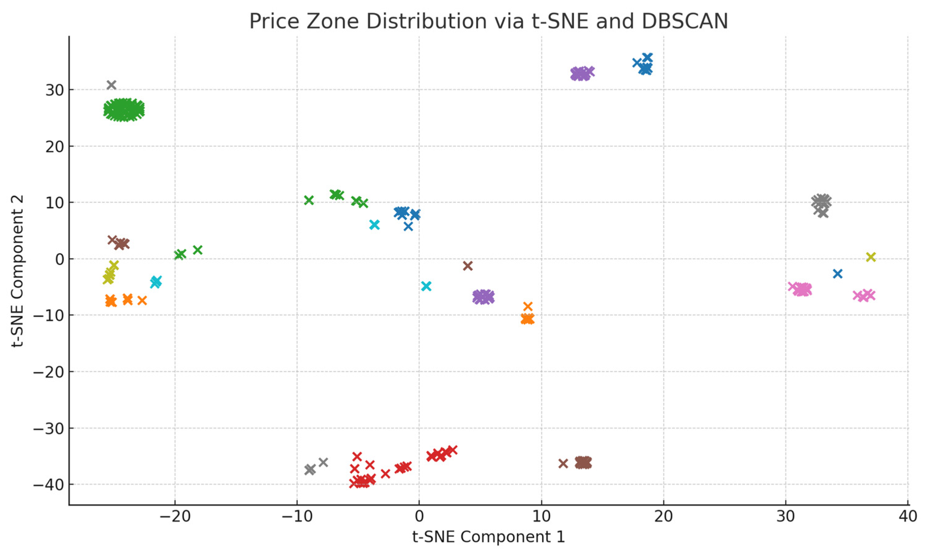
5.1. Selection of Electricity Price Zoning Parameters and Zoning Results

When utilizing the DBSCAN algorithm to partition system node electricity prices, although it can be avoided to determine the number of partitions in advance, the setting of the distance parameter $\epsilon$ and the density threshold parameter $\mathrm{MinPts}$ during the execution of the algorithm will affect the electricity price partitioning results. The electricity price partitioning results of 16 parameter combinations are demonstrated in

Table 1. The effect of electricity price zoning under different parameter combinations.

Gap Parameters $\mathit{\epsilon }$	$\mathbf{Density} \mathbf{Threshold} \mathbf{Parameter}\mathbf{MinPts}$	Number of Electricity Price Divisions	Number of Un-Partitioned Nodes	Range	Interquartile Range	Variance
3	3	43	8	16.87	4.25	4.57
	5	36	36	19.93	4.81	5.26
	10	35	44	20.32	4.94	5.38
	20	28	123	22.90	4.68	5.64
5	3	29	2	27.55	7.74	7.59
	5	25	26	27.70	5.93	6.79
	10	24	36	28.38	6.15	6.98
	22	23	63	28.65	5.50	6.76
10	3	13	2	52.43	9.63	11.02
	5	13	0	52.03	7.39	12.47
	10	12	0	53.08	7.60	9.65
	20	9	4	66.85	9.31	11.83
20	3	5	0	101.51	14.33	16.01
	5	4	0	109.04	11.24	14.26
	10	4	0	114.46	15.17	16.68
	20	2	0	205.51	21.30	24.60

, which measure the different parameter in terms of the number of electricity price partitions, the number of un-partitioned nodes, the extreme deviation, the quartile deviation, and the variance, respectively. The partitioning effect under different parameter combinations is measured in five aspects, namely, the number of electricity price partitions, the number of un-partitioned nodes, the extreme deviation, the quartile deviation, and the variance.

As can be seen from Table 1, when the distance parameter $\epsilon$ exceeds 10, the extreme deviation, quartile deviation, and variance, which measure the degree of concentration of the data distribution, are significantly improved, and the partition results do not satisfy the principle of “electricity prices of all nodes within the partition are as similar as possible, and the distribution is as centralized as possible” as proposed in the first chapter; however, when the distance parameter $\epsilon$ is equal to 3 or 5, there is not much difference in the degree of data concentration after partitioning, but there is a significant difference in the number of electricity price partitions and the number of nodes that are not partitioned. Considering that the electricity price partition should contain all nodes as much as possible, and at the same time, the electricity price partition should not be too much, leading to excessive partitions, the distance parameter $\epsilon$ is set to 5, and the density threshold parameter $\mathrm{MinPts}$ is set to 3, which strikes a balance between coverage of all nodes and avoiding excessive fragmentation. Under this set of hyperparameter settings, the 2022 electricity price is roughly divided into 29 electricity price partitions. From the results of the electricity price zoning, the overall distribution is still based on the division of administrative regions, while in the economically developed areas, the zoning is also closer due to the more complete degree of grid construction. Some coastal areas will form relatively independent electricity price subdivisions due to the influence of the geographic environment. It can be proved that, in the absence of grid topology information, some network information can be restored through historical node electricity price data, and the resulting electricity price partitioning results, which have a certain degree of authenticity and trustworthiness, can be used for the subsequent identification of spatially anomalous electricity price signals.

In addition to the numerical comparison of parameter combinations, Figure 2 provides a visual demonstration of price zone clustering results using t-SNE dimensionality reduction and DBSCAN. This figure illustrates the emergence of structurally distinct price zones after spatial embedding, confirming the existence of latent clustering structures in the nodal price data.

To select the optimal parameters for DBSCAN, we conducted an exhaustive empirical search across 16 parameter combinations, balancing between partition granularity and coverage (Table 1). The final choice of ε = 5 and $\mathrm{MinPts}$ = 3 reflects a compromise between minimizing noise points and ensuring meaningful zonal separation. For t-SNE, a perplexity value of 30 was used, selected after sensitivity analysis indicated robust clustering performance across values ranging from 10 to 50.

5.2. Comparison of the Effectiveness of Different Spatial Electricity Price Anomaly Signal Identification Methods

This section serves to validate the effectiveness of the proposed method by comparing it against two commonly used baseline algorithms in electricity price anomaly detection.

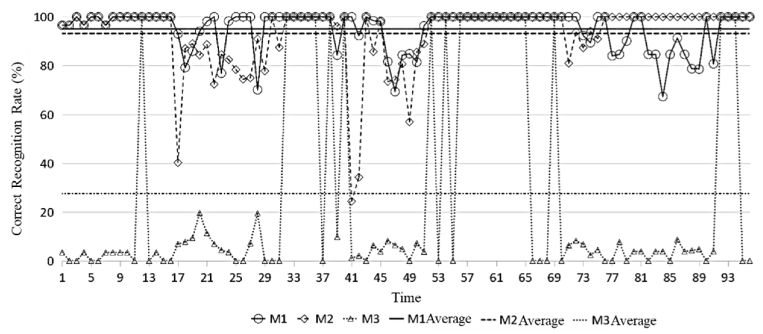
5.2.1. Effectiveness of Spatial Abnormal Electricity Price Identification

Since there is not yet a dedicated method for identifying spatially anomalous electricity price signals, in this section the recognition effects of the proposed method and two commonly used anomalous data recognition methods in the electric power industry on spatially abnormal electricity price signals are compared, and the three methods are shown as follows:

M1: Identification of spatial abnormal electricity price signals proposed in this paper;

M2: Overall identification of spatially abnormal electricity price signals using the Isolated Forest algorithm;

M3: Overall identification of spatially abnormal electricity price signals using the K-means algorithm.

It should be noted that to facilitate the comparison of the recognition effect of different anomalous signals, all the parameter settings of the Isolated Forest algorithm and the data preprocessing process in M2 are consistent with those in M1, and only the partition recognition is no longer carried out. The number of clusters required by the K-means algorithm in M3 is set to be 29, which is the optimal number of partitions obtained in M1, and after clustering, the distances to the center of the clusters exceeding the average distance of the cluster class by more than three times are considered as outliers.

The full-year dataset (96 time intervals per day over 365 days) is used to evaluate the recognition performance of M1, M2, and M3 under consistent settings. The proportion of abnormal electricity price signal points identified by the three methods is shown in

Table 2. The identification ratio of spatial abnormal electricity price signal points for M1–M3.

Methodologies	The Proportion of Anomalous Electricity Price Signal Points Identified
M1	2.06%
M2	6.37%
M3	0.93%

, and the accuracy recognition rate is shown in Figure 3, and the recognition error rate is shown in Figure 4. The accuracy recognition rate refers to the correct number of identified abnormal signals in proportion to the total number of identified abnormal signals by manual recognition. When the number of manually identified abnormal signals is 0, if the method does not detect abnormal signals, the recognition accuracy rate is defined as 100% at this time; if the abnormal signals are detected at this time, the recognition accuracy rate is defined as 0% at this time. The error ratio refers to the number of errors in the identified abnormal signals as a percentage of the total number of identified abnormal signals.

Note that AUC scores were not computed, as the unsupervised nature of the detection framework and the absence of continuous ground-truth probability distributions render ROC-based evaluation metrics inappropriate. Instead, precision, recall, and F1-score offer more interpretable performance insights under a thresholding-based detection setup.

From the data in Table 2, it can be found that the M3 method identifies the least spatially anomalous electricity price signals, which is about one-half of that of the method M1 proposed in this paper, while the M2 method identifies the most spatially anomalous electricity price signals, which is more than three times of that of the method M1 proposed in this paper. To complement the accuracy and error rate evaluation,

Table 3. Confusion matrix-based evaluation metrics.

Methodologies	TP	FP	FN	TN	Precision	Recall	F1-Score	Accuracy
M1	82	11	18	889	0.88	0.82	0.85	0.971
M2	89	52	11	848	0.63	0.89	0.74	0.937
M3	28	65	72	835	0.30	0.28	0.29	0.863

reports additional confusion matrix-based metrics, including precision, recall, and F1-score. These indicators offer a more comprehensive assessment of detection performance across the three methods. Combining the accurate recognition rates of each method in Figure 4, it can be found that compared with the average accurate recognition rate of 95.09% for method M1 and 93.17% for method M2, method M3 has a lower accurate recognition rate of less than 30% on average due to the small number of anomalous signals identified. Meanwhile, although the M1 method and the M2 method have similar recognition accuracy rates, the recognition effect of M1 is smoother compared to that of M2, and the recognition accuracy rate can be maintained at more than 80% in most of the time periods, with no extreme cases.

Combined with the error recognition rate shown in Figure 5, it can be found that M3 has the highest error recognition rate, reaching more than 60% on average, which shows that for K-means, as a specialized clustering algorithm, anomaly recognition is only an accessory function, and the effect is not ideal for the anomaly recognition of unidimensional, non-temporal data such as the whole node electricity price signal. On the other hand, the false recognition rate of the M2 method is more than three times higher than that of the M1 method proposed in this paper, reaching 38.93%. It can be seen that the higher accurate recognition rate of the M2 method relies on a large number of detected anomalous signals to ensure that, although the accurate recognition rate is high, a large number of anomalous signals will be detected incorrectly as well, which will result in too high a false alarm rate. Through the comparison of the recognition effect of the three methods, it can be found that the Isolated Forest algorithm has a certain advantage in the identification of spatial abnormal electricity price signals, but in the case of non-partitioned identification, a large number of electricity price signals that were originally normal within the partition will be recognized as abnormal, resulting in difficulties in the analysis of the causes of the subsequent abnormal electricity price signals. In summary, the method proposed in this paper can ensure the recognition effect of spatial abnormal electricity price signals. To further visualize the spatial–temporal behavior of detected anomalies, Figure 6 shows a node–time anomaly heatmap generated using Isolation Forest. This figure illustrates when and where nodal prices were detected as anomalous across the 96 time intervals, providing insight into the temporal persistence and spatial concentration of outliers.

Table 2 presents the proportion of anomalous electricity price signals identified by each method, while Figure 4 and Figure 5 compare their accuracy and false alarm rates across 96 time intervals. The results validate the effectiveness of the proposed framework: method M1 consistently outperforms the benchmarks by maintaining high accuracy (>80%) and low false alarm rates (<13%) across most time periods. This confirms that incorporating price zone partitioning significantly enhances the precision and reliability of spatial anomaly detection. Moreover, the stability of M1’s performance across time reinforces its robustness under dynamic market conditions, thereby validating the methodological design and its practical applicability. Furthermore, the proposed method demonstrates particular strength in identifying spatially clustered and zone-level anomalies—especially those caused by external factors such as regional congestion, topology reconfiguration, or market behavior shifts. By leveraging structural partitioning, M1 is more sensitive to group-based deviations rather than isolated outliers, enabling the early detection of systemic disturbances that manifest across neighboring nodes.

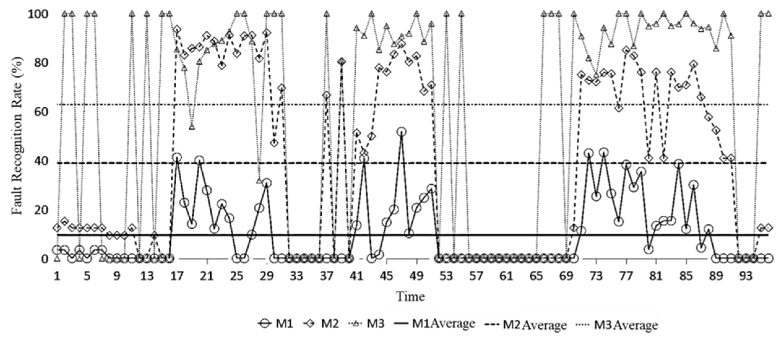
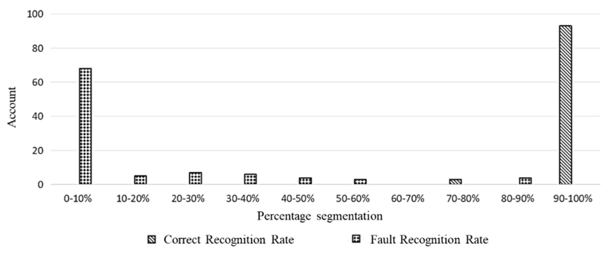
5.2.2. Effectiveness of Electricity Price Anomaly Zoning Identification

The M1 method proposed in this paper can not only complete the identification of abnormal signal points, but also identify regional abnormalities in electricity price signals from the perspective of the market as a whole, so as to further analyze the causes of abnormal electricity price signals. The regional electricity price anomalies are detected for the same-period node electricity price data tested in Section 4.2, and the detection results are shown in Figure 6.

As can be seen from Figure 6, the M1 method proposed in this paper can perfectly recognize all electricity price signal regions in almost all the time periods tested, with an average accuracy of 99.27%. Meanwhile, more than 60% of the time periods have an error recognition rate of less than 10%, and the overall error recognition rate is only 11.72%. Although there is the problem of the over-recognition of abnormal electricity price signal regions, the proportion of extreme misrecognition is very small, while the concentration of regional electricity price distribution is relatively average, and the electricity price data’s sparse characteristics are not obvious in the time period, which needs to be assisted by manual experience to discriminate. These results validate the effectiveness of the proposed two-stage method. By leveraging spatial clustering and localized density analysis, M1 outperforms baseline methods both in terms of accuracy and interpretability, especially in scenarios with complex spatial price structures.

6. Limitations and Computational Considerations

While the proposed method demonstrates high accuracy and interpretability, several limitations should be acknowledged. First, the zoning performance and anomaly detection results are sensitive to hyperparameter selection in both the t-SNE and DBSCAN stages. For example, overly high perplexity values in t-SNE may distort local neighborhood structures, while inappropriate ε or MinPts values in DBSCAN could lead to either over-clustering or excessive noise labeling. Although empirical tuning (e.g., Table 1) provides guidance, a more systematic approach or automated tuning framework (e.g., grid search, Bayesian optimization) could be explored in future studies.

Second, the modular design implies increased computational complexity. In our implementation, the average runtime for DBSCAN on the t-SNE-projected dataset (267 nodes × 35,040 time points) was approximately 15 min on a standard workstation (Intel i7 CPU, 32 GB RAM), while the training of iForest on each price zone typically required 2 s per zone. Although these runtimes are acceptable for offline analysis, real-time deployment may require further acceleration or parallelization.

Finally, the method assumes static price patterns for historical partitioning, which may not fully capture fast-evolving topological changes or policy-induced structural shifts. For example, the emergence of new congestion zones or dynamic renewable integration could introduce new symmetry-breaking patterns not represented in historical data. Addressing such challenges may require adaptive learning mechanisms or the incorporation of exogenous variables (e.g., network topology snapshots, weather conditions).

7. Conclusions

In light of the increasing complexity of electricity markets—driven by the rapid integration of renewable energy—this study presents a novel method for identifying exogenous, spatially asymmetric electricity price anomalies, grounded in the principles of spatial structure and symmetry. By combining dimensionality reduction with unsupervised clustering algorithms, the proposed approach effectively captures latent symmetrical coupling relationships among nodes in historical electricity price data. This facilitates a more granular, structure-aware partitioning of electricity price zones in large-scale power systems, aligning with the natural symmetries embedded in grid topology and market operations. Building on these refined partitions, a two-stage detection framework is developed to identify both nodal-level pricing outliers and asymmetrically distributed abnormal zones, using data sparsity and density deviation as key indicators. In contrast to traditional anomaly detection methods that often overlook spatial dependencies or assume pricing homogeneity, this method explicitly targets spatial deviations that break expected symmetry patterns, thereby enhancing both sensitivity and specificity in anomaly detection.

More importantly, the proposed approach offers a robust foundation for tracing the origins and propagation paths of price anomalies, enabling early warning, regulatory intervention, and market reconfiguration. Its modular and data-driven nature ensures adaptability across diverse electricity market environments, including those undergoing digital transformation, decentralization, or high renewable penetration. By leveraging spatial symmetry-aware partitioning, this method contributes to the development of more transparent, stable, and symmetrically balanced electricity markets. Looking ahead, future research could integrate causal inference models, real-time data streams, and cross-domain sources (e.g., weather conditions, load forecasts, network congestion) to improve predictive capability and anomaly interpretability. The proposed framework also holds promise for integration into intelligent market monitoring platforms, supporting resilient, symmetry-informed electricity market operations in the context of increasing complexity and renewable variability.

While the proposed framework demonstrates promising results, it relies on access to detailed market-clearing data, which may not be available in all regions. Simplifications in the simulation setup—such as static bidding and deterministic inputs—may also limit generalizability. In addition, the current anomaly classification may need expansion to capture more complex scenarios. Nonetheless, the symmetry-based approach and feature attribution mechanism are broadly applicable. It can be adapted to LMP-based markets like PJM and ERCOT, and, with adjustments, to zonal or hybrid systems such as Nord Pool. Its minimal dependence on large datasets makes it particularly suitable for developing or data-limited markets.

References

1. Chen, M.; Xiao, D.; Deng, W.; Tahir, M.F.; Zhu, D. Multi-regional energy sharing approach for shared energy storage and local renewable energy resources considering efficiency optimization. Int. J. Electr. Power Energy Syst. 2025, 167, 110592. [Google Scholar]
2. Ji, T.; Wang, J.; Li, M.; Wu, Q. Short-term wind power forecast based on chaotic analysis and multivariate phase space reconstruction. Energy Convers. Manag. 2022, 254, 115196. [Google Scholar] [CrossRef]
3. Dai, S.; Lin, D.; Liu, Z. Electricity market margin determination method considering the integrity of electricity assets. Energy Rep. 2023, 9, 1259–1267. [Google Scholar] [CrossRef]
4. Lai, W.K.; Wang, Y.C.; Lin, H.C.; Li, J.W. Efficient resource allocation and power control for LTE-A D2D communication with pure D2D model. IEEE Trans. Veh. Technol. 2020, 69, 3202–3216. [Google Scholar] [CrossRef]
5. Qin, M.; Yang, Y.; Zhao, X.; Xu, Q.; Yuan, L. Low-carbon economic multi-objective dispatch of integrated energy system considering the price fluctuation of natural gas and carbon emission accounting. Prot. Control Mod. Power Syst. 2023, 8, 61. [Google Scholar] [CrossRef]
6. Spodniak, P.; Ollikka, K.; Honkapuro, S. The impact of wind power and electricity demand on the relevance of different short-term electricity markets: The Nordic case. Appl. Energy 2021, 283, 116063. [Google Scholar] [CrossRef]
7. Zhang, Q.; Li, F.; Shi, Q.; Tomsovic, K.; Sun, J.; Ren, L. Profit-oriented false data injection on electricity market: Reviews, analyses, and insights. IEEE Trans. Ind. Inform. 2020, 17, 5876–5886. [Google Scholar] [CrossRef]
8. Fabra, N.; Motta, M.; Peitz, M. Learning from electricity markets: How to design a resilience strategy. Energy Policy 2022, 168, 113116. [Google Scholar] [CrossRef]
9. Tschora, L.; Pierre, E.; Plantevit, M.; Robardet, C. Electricity price forecasting on the day-ahead market using machine learning. Appl. Energy 2022, 313, 118752. [Google Scholar] [CrossRef]
10. El-Hadad, R.; Tan, Y.F.; Tan, W.N. Anomaly prediction in electricity consumption using a combination of machine learning techniques. Int. J. Technol. 2022, 13, 1317–1325. [Google Scholar] [CrossRef]
11. Li, Y.; Yu, N.; Wang, W. Machine learning-driven virtual bidding with electricity market efficiency analysis. IEEE Trans. Power Syst. 2021, 37, 354–364. [Google Scholar] [CrossRef]
12. Jain, P.K.; Bajpai, M.S.; Pamula, R. A modified DBSCAN algorithm for anomaly detection in time-series data with seasonality. Int. Arab J. Inf. Technol. 2022, 19, 23–28. [Google Scholar] [CrossRef] [PubMed]
13. Iftikhar, H.; Turpo-Chaparro, J.E.; Canas Rodrigues, P.; López-Gonzales, J.L. Forecasting day-ahead electricity prices for the Italian electricity market using a new decomposition-combination technique. Energies 2023, 16, 6669. [Google Scholar] [CrossRef]
14. Bushnell, J. California’s electricity crisis: A market apart? Energy Policy 2004, 32, 1045–1052. [Google Scholar] [CrossRef]
15. Lee, J.; Cho, Y. National-scale electricity peak load forecasting: Traditional, machine learning, or hybrid model? Energy 2022, 239, 122366. [Google Scholar] [CrossRef]
16. Jan, F.; Shah, I.; Ali, S. Short-term electricity prices forecasting using functional time series analysis. Energies 2022, 15, 3423. [Google Scholar] [CrossRef]
17. Miraftabzadeh, S.M.; Colombo, C.G.; Longo, M.; Foiadelli, F. K-means and alternative clustering methods in modern power systems. IEEE Access 2023, 11, 119596–119633. [Google Scholar] [CrossRef]
18. Liu, X.; Lu, S.; Ren, Y.; Wu, Z. Wind turbine anomaly detection based on SCADA data mining. Electronics 2020, 9, 751. [Google Scholar] [CrossRef]
19. Lin, C.; Han, G.; Wang, T.; Bi, Y.; Du, J.; Zhang, B. Fast node clustering based on an improved birch algorithm for data collection towards software-defined underwater acoustic sensor networks. IEEE Sens. J. 2021, 21, 25480–25488. [Google Scholar] [CrossRef]
20. He, Q.; Wang, H.; Li, C.; Zhou, W.; Ye, Z.; Hong, L.; Yu, X.; Yu, S.; Peng, L. A Clone Selection Algorithm Optimized Support Vector Machine for AETA Geoacoustic Anomaly Detection. Electronics 2023, 12, 4847. [Google Scholar] [CrossRef]
21. Ambrosius, M.; Grimm, V.; Kleinert, T.; Liers, F.; Schmidt, M.; Zöttl, G. Endogenous price zones and investment incentives in electricity markets: An application of multilevel optimization with graph partitioning. Energy Econ. 2020, 92, 104879. [Google Scholar] [CrossRef]
22. Bernardi, M.; Lisi, F. Point and interval forecasting of zonal electricity prices and demand using heteroscedastic models: The IPEX case. Energies 2020, 13, 6191. [Google Scholar] [CrossRef]
23. Kontopoulou, V.I.; Panagopoulos, A.D.; Kakkos, I.; Matsopoulos, G.K. A review of ARIMA vs. machine learning approaches for time series forecasting in data driven networks. Future Internet 2023, 15, 255. [Google Scholar] [CrossRef]
24. Retiti Diop Emane, C.; Song, S.; Lee, H.; Choi, D.; Lim, J.; Bok, K.; Yoo, J. Anomaly detection based on GCNs and DBSCAN in a large-scale graph. Electronics 2024, 13, 2625. [Google Scholar] [CrossRef]
25. Savitski, D.W. LMPs for (Technically-Inclined) Dummies. Energy Law J. 2019, 40, 165–208. [Google Scholar]
26. Jain, M.; Sun, X.; Datta, S.; Somani, A. A Machine Learning Framework to Deconstruct the Primary Drivers for Electricity Market Price Events. arXiv 2023, arXiv:2309.06082. [Google Scholar]
27. Dvorkin, V.; Fioretto, F. Price-Aware Deep Learning for Electricity Markets. arXiv 2023, arXiv:2308.01436. [Google Scholar]
28. Yang, Y.S.; Xie, B.C.; Tan, X. Impact of Green Power Trading Mechanism on Power Generation and Interregional Transmission in China. Energy Policy 2024, 189, 114088. [Google Scholar] [CrossRef]
29. Owolabi, O.O.; Schafer, T.L.; Smits, G.E.; Sengupta, S.; Ryan, S.E.; Wang, L.; Sunter, D.A. Role of variable renewable energy penetration on electricity price and its volatility across independent system operators in the United States. Data Sci. Sci. 2023, 2, 2158145. [Google Scholar] [CrossRef]
Figure 1. Flowchart of sub-area identification method of spatial abnormal electricity price.
Symmetry 17 01032 g001
Figure 2. t-SNE projection of electricity price vectors followed by DBSCAN clustering. Each color represents a distinct price zone identified through unsupervised clustering, where spatially concentrated points indicate similar pricing behaviors.
Symmetry 17 01032 g002
Figure 3. Accurate identification rate of spatial abnormal electricity price signals for M1–M3.
Symmetry 17 01032 g003
Figure 4. Spatial abnormal electricity price signal misidentification rate for M1–M3.
Symmetry 17 01032 g004
Figure 5. Node–time anomaly heatmap generated via Isolation Forest.
Symmetry 17 01032 g005
Figure 6. The effectiveness of M1 in identifying abnormal electricity price zones.
Symmetry 17 01032 g006