Confidence Intervals for the Parameter Mean of Zero-Inflated Two-Parameter Rayleigh Distribution

Abstract

The Rayleigh distribution is a continuous probability distribution that is inherently asymmetric and commonly used to model right-skewed data. It holds significant importance across a wide range of scientific and engineering disciplines and exhibits structural relationships with several other asymmetric probability distributions, for example, Weibull and exponential distribution. This research proposes techniques for establishing credible intervals and confidence intervals for the single mean of the zero-inflated two-parameter Rayleigh distribution. The study introduces methods such as the percentile bootstrap, generalized confidence interval, standard confidence interval, approximate normal using the delta method, Bayesian credible interval, and Bayesian highest posterior density. The effectiveness of the proposed methods is assessed by evaluating coverage probability and expected length through Monte Carlo simulations. The results indicate that the Bayesian highest posterior density method outperforms the other approaches. Finally, the study applies the proposed methods to construct confidence intervals for the single mean using real-world data on COVID-19 total deaths in Singapore during October 2022.

1. Introduction

Characterized by its asymmetry, the Rayleigh distribution is a continuous probability model particularly effective for describing data with a pronounced right skew. In various fields, it is common to analyze data comprising values greater than zero, such as mortality rates, the number of deaths caused by diseases, or fatalities resulting from accidents. Such data are characteristically asymmetric due to the presence of a long right tail, indicating that although extreme values may be observed, they occur infrequently. The Rayleigh distribution was first introduced by Rayleigh [1]. It is extensively applied in various fields, including medical research, quality control, and reliability engineering. For example, Arikan et al. [2] explored the power of wind energy, optimal turbine selection, and associated costs in Turkey using the Rayleigh distribution. Similarly, Almongy et al. [3] analyzed real mortality rate data from COVID-19 in Italy, Mexico, and the Netherlands across different time periods. Kilai et al. [4] used the Rayleigh distribution to study mortality rates from COVID-19 data in Italy and Canada. Kilany et al. [5] applied the power Rayleigh distribution to describe hydrologic data and the total COVID-19 deaths in Egypt. Finally, Seal et al. [6] analyzed the strength of carbon fibers, measured in Giga-Pascals, and applied the findings to predict the lifetime of T8 fluorescent lamps.

In statistical inference, describing unknown parameters of a distribution is crucial for certain fields that rely on accurate forecasting. Numerous studies have applied statistical inference to various fields, including public health, reliability, and degradation modeling. Xu et al. [7] propose a novel class of tail-weighted multivariate degradation models and demonstrate their application using two real-world degradation datasets. Xu et al. [8] explore adaptive sampling and ensemble techniques for estimating the remaining useful life of machinery, which significantly contributes to operational efficiency and cost-effective maintenance. Li et al. [9] introduced a Bayesian hierarchical model designed for public health applications, validated with data from mouse brain research and studies on human pancreatic ductal adenocarcinoma. Ma et al. [10] developed a new algorithm for statistical inference aimed at estimating parameters in regression models, with an application to chemical sensor data. The two unknown parameters of the two-parameter Rayleigh distribution are the location and scale parameters, which describe the characteristics of the distribution. There are various methods used to estimate unknown parameters, with popular methods including the maximum likelihood method and Bayesian method. Dey et al. [11] considered various methods for estimating unknown parameters, including point estimation using maximum likelihood, the method of moments, L-moments, percentile-based estimates, the least squares method, and Bayesian estimation. The Bayesian estimation process utilized a gamma prior to model the scale parameter and a uniform prior for the location parameter. Ardianti and Sutarman [12] estimated the parameter for one parameter Rayleigh distribution using maximum likelihood and Bayesian estimate under non-informative prior. El-Faheem et al. [13] proposed reliability function and estimate parameters for Rayleigh distribution with two parameters using maximum likelihood, the first and second modified method of moment and Bayesian estimate. Krishnamoorthy et al. [14] developed various confidence intervals based on the method of pivotal quantities for mean. Seal et al. [6] proposed estimation in Rayleigh distribution using Bayesian estimation under a distance-type loss function. For distributions characterized by an excess of zeros, the concept of zero-inflated modeling was first introduced by Lambert [15]. Subsequently, this concept has been extended to various distributions, leading to the development of zero-inflated versions of well-known models. In particular, the Rayleigh distribution has been modified to incorporate zero inflation. Fuxiang et al. [16] proposed a zero-inflated Rayleigh distribution with a single parameter, introducing its probability distribution function and methods for estimating parameters. Since then, numerous studies have developed confidence intervals for zero-inflated models based on various underlying distributions. For example, Maneerat et al. [17] suggested approaches for developing confidence intervals for lognormal distribution means with certain zero values. It is called delta lognormal, and it uses a variance estimates recovery approach and generalized confidence interval. It is demonstrated through applications using two real datasets: the abundance of red cod in the waters of New Zealand and airborne chlorine in the United States.

Additionally, only a few studies have explored methods for inferring parameters of the two-parameter Rayleigh distribution. For example, the study by Seo et al. [18] constructed an exact confidence interval for a two-parameter Rayleigh distribution, while Teawpongpan and Sangnawakij [19] initiated the proposal for estimating the mean for one parameter Rayleigh distribution using confidence intervals through the large sample method. This research is the first to introduce a methodology for constructing confidence intervals for the single mean of the zero-inflated two-parameter Rayleigh distribution. It builds upon the work of Kilai et al. [4], who applied the Rayleigh distribution to model the mortality rate of COVID-19. Our work differs from previous studies in that we have developed a zero-inflated version of the distribution to improve the accuracy and effectiveness of mean estimation in practical applications. Elshahhat [20] proposed a new joint Type-I hybrid censoring scheme for comparing the lifetimes of products from two production lines based on the one-parameter Rayleigh distribution. Maximum likelihood and Bayesian methods were employed to analyze the censored data, and the performance was evaluated through simulations and real engineering data. Ahmad et al. [21] introduced a generalized Rayleigh distribution that provides enhanced flexibility for modeling lifetime data. The study explores several statistical properties, applies maximum likelihood estimation (MLE) for parameter inference, and demonstrates the model’s effectiveness through real data applications. Shen et al. [22] proposes a new extended generalized Rayleigh distribution with heavy-tailed characteristics, applied to Reddit advertising and breast cancer datasets. Parameters are estimated using maximum likelihood, and the model’s performance is compared with other Rayleigh-type distributions.

This paper focuses on constructing credible interval and confidence intervals for the single mean of a zero-inflected two-parameter Rayleigh distribution. Six different methods are utilized for parameter estimation: the percentile bootstrap method, the generalized confidence interval, the standard confidence interval based on maximum likelihood estimation, the approximate normal method based on the delta method, the Bayesian credible interval, and the Bayesian highest posterior density. In the Bayesian approach for estimating the single mean, the scale parameter is assigned a gamma prior, while the location parameter is assigned a uniform prior. Coverage probability and expected length were used to evaluate the effectiveness of the proposed credible and confidence intervals, both derived through Monte Carlo simulations conducted using R version 4.4.1 and OpenBUGS version 3.2.3. In the Section 4, total death data collected by the WHO for Singapore in October 2022 were used to estimate confidence intervals for the mean.

The remainder of this paper is organized as follows. Section 2 introduces the zero-inflated two-parameter Rayleigh distribution and details the proposed interval estimation methods. Section 3 presents the results of the simulation study. Section 4 illustrates the application of the proposed methods to real data, and Section 5 concludes the paper with a summary and recommendations for future applications.

2. Materials and Methods

Let $\left(x_1,x_2,\dots ,x_n\right)$ represent a set of observations drawn independently from a zero-inflated two-parameter Rayleigh distribution, denoted by $ZITR(\mu ,\lambda ,\delta )$. The probability density function of this distribution is defined as follows:

$$f\left(x;\mu ,\lambda ,\delta \right)=\left\{\begin{array}{c}\delta ;x=0\\ (1-\delta )2\lambda (\mathrm{x}-\mu ){\mathrm{e}}^{-\lambda {\left(x-\mu \right)}^2};x>\mu ,\end{array}\right.$$

(1)

where $\lambda$, which is greater than zero, represents the scale parameter of the Rayleigh distribution, and $\mu$ is the location parameter. The probability of zeros is given by the parameter $\delta$. The maximum likelihood method can be used to estimate the parameters $\mu$, $\lambda$, and $\delta$. However, closed-form solutions are not available for $\mu$ and $\lambda$. Dey et al. [11] and Krishnamoorthy et al. [14] proposed calculating the MLEs of $\mu$ and $\lambda$ using numerical approaches. The maximum likelihood estimator for $\mu$ is obtained by solving the following equation: ${\displaystyle \frac{2n_1^2\left(\overline{x}-\mu \right)}{{\displaystyle \sum _{i=1}^{n_1}}{\left(x_i-\mu \right)}^2}}-{\displaystyle \sum _{i=1}^{n_1}}{\left(x_i-\mu \right)}^{-1}=0$, while the MLE of $\lambda$ is given by $\widehat{\lambda }={\displaystyle \frac{n_1}{{\displaystyle \sum _{i=1}^{n_1}}{(x_i-\widehat{\mu })}^2}}$. The estimator for $\delta$ is given by $\widehat{\delta }={\displaystyle \frac{n_0}{n}}$. $n_0$ is the number of zeros in the sample of size n, and $n_1=n-n_0$. The distribution expectation is defined by

$$\psi =\left(1-\delta \right)\left(\mu +{\displaystyle \frac{1}{\sqrt{\lambda }}}\Gamma \left({\displaystyle \frac{3}{2}}\right)\right).$$

(2)

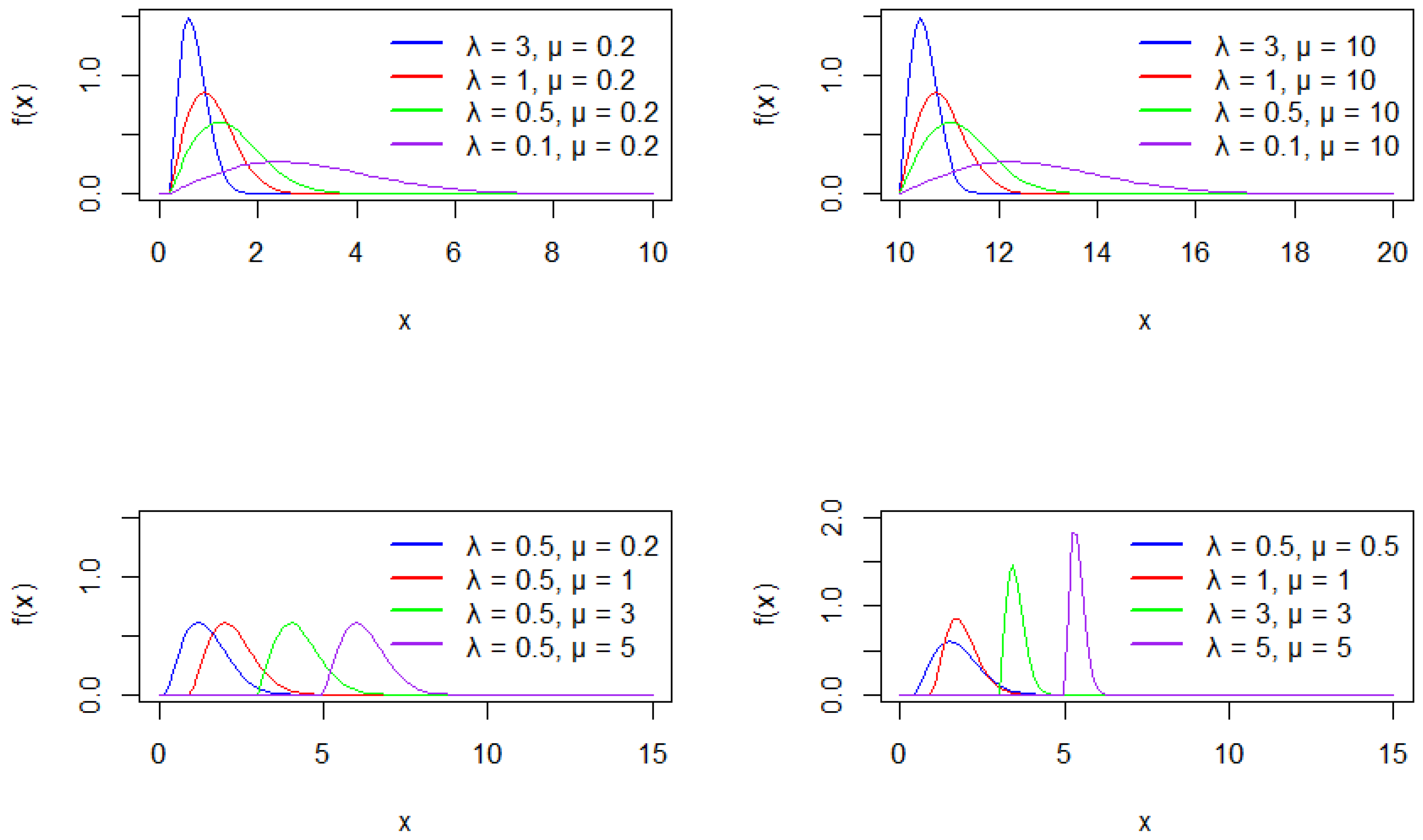
The two-parameter Rayleigh distribution is employed in this study for its greater flexibility in modeling data with fast-aging behavior. Figure 1 shows how the distribution’s shape varies with different parameter values.

2.1. The Percentile Bootstrap Confidence Interval

The concept was first introduced by Efron and Tibshirani [23], where the bootstrap confidence interval relies on percentile-based replication of the target distribution. The mean can be estimated using Equation (2), and a two-sided percentile bootstrap confidence interval for the mean of the zero-inflated two-parameter Rayleigh distribution can be constructed as shown in Equation (3):

$$C{I}_{\psi \left(PB\right)}=\left(L_{\psi \left(PB\right)},U_{\psi \left(PB\right)}\right)=\left({\widehat{\psi }}^{\ast b}\left(\alpha /2\right),{\widehat{\psi }}^{\ast b}\left(1-\alpha /2\right)\right),$$

(3)

where ${\widehat{\psi }}^{\ast b}\left(\alpha \right)$ represent the $100\left(\alpha \right)\%$ percentile of ${\widehat{\psi }}^{\ast b}$. The confidence interval for the single mean of zero-inflated two-parameter Rayleigh distribution based on percentile bootstrap is constructed according to Algorithm 1.

Algorithm 1 The percentile bootstrap method

Generate random sample $x\sim ZITR(\mu ,\lambda ,\delta )$. Resample $x_i^{\ast b}=\left(x_1^{\ast b},x_2^{\ast b}\dots x_n^{\ast b}\right)$ from original data $x=\left(x_1,\dots x_n\right)$ for using same sample. Compute ${\widehat{\mu }}^{\ast b},{\widehat{\lambda }}^{\ast b}$, and ${\widehat{\delta }}^{\ast b}$ using maximum likelihood. Compute ${\widehat{\psi }}^{\ast b}$ from Equation (2). Perform steps 2–4 for B iterations, where B represents the resampling value in the bootstrap method. Arrange ${\widehat{\psi }}^{\ast b}$ in ascending. Compute 95% percentile bootstrap interval, as given by Equation (3).

2.2. The Generalized Confidence Interval (GCI)

The first idea for the generalized confidence interval (GCI) was proposed by Weerahandi [24], and it is grounded in the concept of the generalized pivotal quantity (GPQ). Building on this foundation, the concepts of the pivotal quantity and its generalized form (GPQ) differ fundamentally. While a pivotal quantity is constructed based on the sampling distribution and the parameters of interest, a GPQ incorporates nuisance parameters into its formulation. However, these nuisance parameters do not affect the observed value of the GPQ. Importantly, the GPQ method involves quantities whose distributions are free from unknown parameters, making them suitable for inference even in complex models.

Krishnamoorthy et al. [14] proposed pivotal quantities specifically for the unknown parameters of the two-parameter Rayleigh distribution. The parameters are represented as a = $\mu$ and $\lambda ={\displaystyle \frac{1}{2b^2}}$.

Let ${\widehat{a}}_0$ and ${\widehat{b}}_0$ be observed values of $\widehat{a}$ and $\widehat{b}$, respectively. The pivotal quantities for the parameters are given by

$${\displaystyle \frac{\widehat{a}-a}{b}}\sim {\widehat{a}}^{\ast },$$

(4)

and

$${\displaystyle \frac{\widehat{b}}{b}}\sim {\widehat{b}}^{\ast },$$

(5)

where $\widehat{a}$ and $\widehat{b}$ are the maximum likelihood estimates from the two-parameter Rayleigh distribution with a = 0 and b = 1, based on a sample of size n. The pivotal quantities for a and b follow the distribution of

$$Q_a=\widehat{a}-\widehat{b}{\displaystyle \frac{{\widehat{a}}^{\ast }}{{\widehat{b}}^{\ast }}},$$

(6)

and

$$Q_b={\displaystyle \frac{\widehat{b}}{{\widehat{b}}^{\ast }}}.$$

(7)

Thus, the pivotal quantity for $\lambda$ is defined as $Q_a=Q_{\mu }$ and $Q_{\lambda }=$ ${\displaystyle \frac{1}{2{Q_b}^2}}$. Furthermore, Wu and Hsieh [25] construct the pivotal quantities based on VST to construct intervals, which is

$$Q_{\delta }={sin}^2\left(arcsin\sqrt{\widehat{\delta }}-{\displaystyle \frac{T}{2\sqrt{n}}}\right),$$

(8)

where $T=2\sqrt{n}\left(arcsin\sqrt{\widehat{\delta }}-arcsin\sqrt{\delta }\right)\sim N(0,1)$. Hence, considering the three pivotal $Q_a$, $Q_{\lambda }$, and $Q_{\delta }$, which are independent of the parameter values, GPQ for the mean of the zero-inflated Rayleigh distribution is given by

$$Q_{\psi }=\left(1-Q_{\delta }\right)\left(Q_{\mu }+{\displaystyle \frac{1}{\sqrt{Q_{\lambda }}}}\Gamma \left({\displaystyle \frac{3}{2}}\right)\right).$$

(9)

Therefore, GCI for the single mean of the zero-inflated Rayleigh distribution is given by Equation (10):

$$C{I}_{\psi \left(GCI\right)}=\left(L_{\psi \left(GCI\right)},U_{\psi \left(GCI\right)}\right)=\left(Q_{\psi }\left(\alpha /2\right),Q_{\psi }\left(1-\alpha /2\right)\right).$$

(10)

The confidence intervals for the single mean of the zero-inflated two-parameter Rayleigh distribution, based on the GCI method, are constructed according to Algorithm 2.

Algorithm 2 The GCI method

Generate random sample $x\sim ZITR(\mu ,\lambda ,\delta )$. Compute $\widehat{a}$ and $\widehat{b}$ from MLE. Generate $x^{\ast }=\left({x_1}^{\ast },{x_2}^{\ast },\dots ,{x_n}^{\ast }\right)$ from two-parameter Rayleigh distribution $\left(a=0,b=1\right)$ or two-parameter Rayleigh distribution $\left(\mu =0,\lambda =0.5\right)$. Compute ${\widehat{a}}^{\ast }$ and ${\widehat{b}}^{\ast }$ from MLE. Compute $Q_{\delta }$, $Q_{\mu }$, $Q_{\lambda }$ and $Q_{\psi }$. Compute $Q_{\psi }$. Perform steps 3–6 repeatedly for q times, where q represents the number of generalized computations. Arrange $Q_{\psi }$ in ascending. Evaluate 95% GCI. As given by Equation (10).

2.3. Standard Confidence Interval Based on Maximum Likelihood

The standard confidence interval is a basic method for estimating confidence intervals of parameters. The method for the parameters of the two-parameter Rayleigh distribution was first proposed by Dey et al. [11].

Let $x=\left(x_1,\dots x_n\right)$ represent observation drawn independently with sample size n. The approximate confidence interval of $\delta ,\lambda$, and $\mu$ are given as follows:

$$C{I}_{\delta \left(MLE\right)}=\left(L_{\delta },U_{\delta }\right)=\left(\widehat{\delta }-z_{1-\alpha /2}\sqrt{{\displaystyle \frac{\widehat{\delta }\left(1-\widehat{\delta }\right)}{n}}},\widehat{\delta }+z_{1-\alpha /2}\sqrt{{\displaystyle \frac{\widehat{\delta }\left(1-\widehat{\delta }\right)}{n}}}\right),$$

(11)

$$C{I}_{\lambda \left(MLE\right)}=\left(L_{\lambda },U_{\lambda }\right)=\left(\widehat{\lambda }-z_{1-\alpha /2}{\displaystyle \frac{\widehat{\lambda }}{\sqrt{n}}},\widehat{\lambda }+z_{1-\alpha /2}{\displaystyle \frac{\widehat{\lambda }}{\sqrt{n}}}\right),$$

(12)

and

$$C{I}_{\mu \left(MLE\right)}=\left(L_{\mu },U_{\mu }\right)=\left(\widehat{\mu }-z_{1-\alpha /2}{\left({\displaystyle \frac{1}{2\widehat{\mu }+\frac{1}{n}{\sum }_{i=1}^n{\left(x_i-\widehat{\mu }\right)}^{-2}}}\right)}^{{\displaystyle \frac{1}{2}}},\widehat{\mu }+z_{1-\alpha /2}{\left({\displaystyle \frac{1}{2\widehat{\mu }+\frac{1}{n}{\sum }_{i=1}^n{\left(x_i-\widehat{\mu }\right)}^{-2}}}\right)}^{{\displaystyle \frac{1}{2}}}\right),$$

(13)

where $\widehat{\delta },\widehat{\lambda }$, and $\widehat{\mu }$ are the maximum likelihood estimators from random samples, and the standard confidence interval for the single mean, based on the maximum likelihood estimators, is constructed using Equation (14):

$$C{I}_{\psi \left(MLE\right)}=\left(L_{\psi \left(MLE\right)},U_{\psi \left(MLE\right)}\right)=\left(\left(1-L_{\delta }\right)\left(L_{\mu }+{\displaystyle \frac{1}{\sqrt{L_{\lambda }}}}\Gamma \left({\displaystyle \frac{3}{2}}\right)\right),\left(1-U_{\delta }\right)\left(U_{\mu }+{\displaystyle \frac{1}{\sqrt{U_{\lambda }}}}\Gamma \left({\displaystyle \frac{3}{2}}\right)\right)\right).$$

(14)

The standard confidence interval for the mean of the zero-inflated Rayleigh distribution based on the maximum likelihood method is constructed according to Algorithm 3.

Algorithm 3 The standard confidence interval method

Generate random sample $x\sim ZITR(\mu ,\lambda ,\delta )$. Estimation parameters $\widehat{\delta },\widehat{\lambda }$, and $\widehat{\mu }$ by using maximum likelihood. Compute the confidence intervals for parameter. $\delta ,\lambda$, and $\mu$ from Equations (11)–(13) Compute $\psi$ from Equation (2). Compute the single mean $\psi$ standard confidence interval using the maximum likelihood method from Equation (14).

2.4. Approximation Normal for Confidence Interval Based on Delta Method

The delta method is a technique within the framework of normal approximation used to obtain a normal distribution as the limiting distribution of an estimator. This common approach is summarized as follows:

Suppose that $g\left(u_1,u_2,u_3\right)$ is a differentiable scalar function with parameters of interest. For the estimator $G\left(U_1,U_2,U_3\right)$, the objective is to identify the asymptotic distribution of G by constructing a stochastic representation. The delta method is applied to confirm the asymptotic normality of G as the sample size tends to infinity, enabling the calculation of the asymptotic mean and variance of $\psi$. In Equation (15), the function g is expanded into Taylor series at ${\theta }_1,{\theta }_2,{\theta }_3$, the true values corresponding to $U_1,U_2,U_3$.

$$g\left(U_1,U_2,U_3\right)\approx g\left({\theta }_1,{\theta }_2,{\theta }_3\right)+{\displaystyle \frac{\partial g\left({\theta }_1,{\theta }_2,{\theta }_3\right)}{\partial u_1}}\left(U_1-{\theta }_1\right)+{\displaystyle \frac{\partial g\left({\theta }_1,{\theta }_2,{\theta }_3\right)}{\partial u_2}}\left(U_2-{\theta }_2\right)+{\displaystyle \frac{\partial g\left({\theta }_1,{\theta }_2,{\theta }_3\right)}{\partial u_3}}\left(U_3-{\theta }_3\right).$$

(15)

The basic statistics are assumed here as $U_1=\widehat{\delta },U_2=\widehat{\mu }$ and $U_3=\widehat{\lambda }$, where $\widehat{\delta },\widehat{\mu },\widehat{\lambda }$ are the MLE of $\delta ,\mu ,\lambda$ respectively. Then, $\widehat{\psi }=g\left(\widehat{\delta },\widehat{\mu },\widehat{\lambda }\right)$, where the function $\psi ={\delta }^{\prime }\left(\mu +{\displaystyle \frac{1}{\sqrt{\lambda }}}\Gamma \left({\displaystyle \frac{3}{2}}\right)\right)$. The partial derivatives are as follows:

$${\displaystyle \frac{\partial }{\partial \delta }}g\left(\delta ,\lambda ,\mu \right)=\left(-1\right)\left(\mu +{\displaystyle \frac{1}{{\lambda }^{\frac{1}{2}}}}\Gamma \left({\displaystyle \frac{3}{2}}\right)\right),$$

$${\displaystyle \frac{\partial }{\partial \mu }}g\left(\delta ,\lambda ,\mu \right)=\left(1-\delta \right),$$

$${\displaystyle \frac{\partial }{\partial \lambda }}g\left(\delta ,\lambda ,\mu \right)=\left(1-\delta \right)\left(-{\displaystyle \frac{1}{2}}{\lambda }^{-{\displaystyle \frac{3}{2}}}\Gamma \left({\displaystyle \frac{3}{2}}\right)\right).$$

Therefore, the expression for $\widehat{\psi }$ is derived using Taylor series expansion of the function $g\left(\delta ,\mu ,\lambda \right)$ around the true parameter values. This approximation linearizes the function with respect to the parameter estimates $\widehat{\delta },\widehat{\lambda }$, and $\widehat{\mu }$ given by   

$\widehat{\psi }\approx g\left(\delta ,\mu ,\lambda \right)+{\displaystyle \frac{\partial }{\partial \delta }}g\left(\delta ,\lambda ,\mu \right)\left(\widehat{\delta }-\delta \right)+{\displaystyle \frac{\partial }{\partial \mu }}g\left(\delta ,\lambda ,\mu \right)\left(\widehat{\mu }-\mu \right)+{\displaystyle \frac{\partial }{\partial \lambda }}g\left(\delta ,\lambda ,\mu \right)\left(\widehat{\lambda }-\lambda \right)$.

The approximate mean and variance for $\widehat{\psi }$ can be derived by considering the expectation and variance given by   

$E\left(\widehat{\psi }\right)=E\left(\psi +\left(-1\right)\left(\mu +{\displaystyle \frac{1}{{\lambda }^{\frac{1}{2}}}}\Gamma \left({\displaystyle \frac{3}{2}}\right)\right)\left(\widehat{\delta }-\delta \right)+\left(1-\delta \right)\left(\widehat{\mu }-\mu \right)+\left(1-\delta \right)\left(-{\displaystyle \frac{1}{2}}{\lambda }^{-{\displaystyle \frac{3}{2}}}\Gamma \left({\displaystyle \frac{3}{2}}\right)\right)\left(\widehat{\lambda }-\lambda \right)\right)$,

$E\left(\widehat{\psi }\right)=\left(E\left(\psi \right)+\left(-1\right)\left(\mu +{\displaystyle \frac{1}{{\lambda }^{\frac{1}{2}}}}\Gamma \left({\displaystyle \frac{3}{2}}\right)\right)E\left(\widehat{\delta }-\delta \right)+\left(1-\delta \right)E\left(\widehat{\mu }-\mu \right)+\left(1-\delta \right)\left(-{\displaystyle \frac{1}{2}}{\lambda }^{-{\displaystyle \frac{3}{2}}}\Gamma \left({\displaystyle \frac{3}{2}}\right)\right)E\left(\widehat{\lambda }-\lambda \right)\right)$,

$E\left(\widehat{\psi }\right)=\psi$,

$V\left(\widehat{\psi }\right)\approx V\left(\psi +\left(-1\right)\left(\mu +{\displaystyle \frac{1}{{\lambda }^{\frac{1}{2}}}}\Gamma \left({\displaystyle \frac{3}{2}}\right)\right)\left(\widehat{\delta }-\delta \right)\right.$

$\left.+\left(1-\delta \right)\left(\widehat{\mu }-\mu \right)+\left(1-\delta \right)\left(-{\displaystyle \frac{1}{2}}{\lambda }^{-{\displaystyle \frac{3}{2}}}\Gamma \left({\displaystyle \frac{3}{2}}\right)\right)\left(\widehat{\lambda }-\lambda \right)\right)$

   $={\left(-1\right)}^2{\left(\mu +{\displaystyle \frac{1}{{\lambda }^{\frac{1}{2}}}}\Gamma \left({\displaystyle \frac{3}{2}}\right)\right)}^{2}V\left(\widehat{\delta }-\delta \right)+{\left(1-\delta \right)}^{2}V\left(\widehat{\mu }-\mu \right)+{\left(1-\delta \right)}^2{\left(-{\displaystyle \frac{1}{2}}{\lambda }^{-{\displaystyle \frac{3}{2}}}\Gamma \left({\displaystyle \frac{3}{2}}\right)\right)}^{2}V\left(\widehat{\lambda }-\lambda \right)$.   

Thus, as $n\to \infty$, $\widehat{\psi }$ is approximately normally distributed with mean $E\left(\widehat{\psi }\right)$ and variance $V\left(\widehat{\psi }\right)$. The estimations of the variances $V\left(\widehat{\lambda }-\lambda \right)$ and $V\left(\widehat{\mu }-\mu \right)$ for the two-parameter Rayleigh distribution were presented in the study by Dey S. et al. [11], and the results are given as follows: $V\left(\widehat{\lambda }-\lambda \right)={\displaystyle \frac{{\lambda }^2}{n}}$ and $V\left(\widehat{\mu }-\mu \right)\approx {\displaystyle \frac{1}{2\mu +\frac{1}{n}{\displaystyle \sum _{i=1}^n}{\left(x_i-\mu \right)}^{-2}}}$. We use plug-in estimators for $E\left(\widehat{\psi }\right)$ and $V\left(\widehat{\psi }\right)$ as follows:

$$V\left(\widehat{\psi }\right)={\left(\mu +{\displaystyle \frac{1}{{\lambda }^{\frac{1}{2}}}}\Gamma \left({\displaystyle \frac{3}{2}}\right)\right)}^2{\displaystyle \frac{\delta \left(1-\delta \right)}{n}}+{\left(1-\delta \right)}^2{\displaystyle \frac{1}{2\mu +\frac{1}{n}{\displaystyle \sum _{i=1}^n}{\left(x_i-\mu \right)}^{-2}}}+{\left(1-\delta \right)}^2{\left(-{\displaystyle \frac{1}{2}}{\lambda }^{-{\displaystyle \frac{3}{2}}}\Gamma \left({\displaystyle \frac{3}{2}}\right)\right)}^2{\displaystyle \frac{{\lambda }^2}{n}}.$$

(16)

The estimate of $V\left(\widehat{\psi }\right)$ is as follows:

$$\widehat{V}\left(\widehat{\psi }\right)={\left(\widehat{\mu }+{\displaystyle \frac{1}{{\widehat{\lambda }}^{\frac{1}{2}}}}\Gamma \left({\displaystyle \frac{3}{2}}\right)\right)}^2{\displaystyle \frac{\widehat{\delta }\left(1-\widehat{\delta }\right)}{n}}+{\left(1-\widehat{\delta }\right)}^2{\displaystyle \frac{1}{2\widehat{\mu }+\frac{1}{n_1}{\displaystyle \sum _{i=1}^{n_1}}{\left(x_{1i}-\widehat{\mu }\right)}^{-2}}}+{\left(1-\widehat{\delta }\right)}^2{\left(-{\displaystyle \frac{1}{2}}{\widehat{\lambda }}^{-{\displaystyle \frac{3}{2}}}\Gamma \left({\displaystyle \frac{3}{2}}\right)\right)}^2{\displaystyle \frac{{\widehat{\lambda }}^2}{n_1}}.$$

(17)

where $x_{1i}$ represents positive observation from the two-parameter Rayleigh distribution, and let $n_1$ denotes the number of observations with values greater than zero.

Therefore, the confidence interval for the approximate normal is based on the delta method for the single mean constructed by Equation (18):

$$C{I}_{\psi \left(AN\right)}=\left(L_{\psi \left(AN\right)},U_{\psi \left(AN\right)}\right)=\left(\widehat{\psi }-z_{1-\alpha /2}\sqrt{\widehat{V}\left(\widehat{\psi }\right)},\widehat{\psi }+z_{1-\alpha /2}\sqrt{\widehat{V}\left(\widehat{\psi }\right)}\right),$$

(18)

where $\widehat{\psi }=\left(1-\widehat{\delta }\right)\left(\widehat{\mu }+{\displaystyle \frac{1}{{\widehat{\lambda }}^{\frac{1}{2}}}}\Gamma \left({\displaystyle \frac{3}{2}}\right)\right)$, with $\widehat{\delta },\widehat{\lambda }$, and $\widehat{\mu }$ being the maximum likelihood estimators. The variance of $\widehat{\psi }$ denoted by $V\left(\widehat{\psi }\right)$ is estimated using the delta method and computed according to Equation (16). The confidence interval for the mean of the zero-inflated two-parameter Rayleigh distribution, based on approximate normality from the delta method, is constructed according to Algorithm 4.

Algorithm 4 The approximation normal method

Generate random sample $x\sim ZITR(\mu ,\lambda ,\delta )$. Estimation parameters $\widehat{\delta },\widehat{\lambda }$, and $\widehat{\mu }$ by using maximum likelihood. Compute variance for $\widehat{\psi }$ based on the delta method from Equation (17). Evaluate the confidence interval for $\psi$ by utilizing the delta method with the approximate normal distribution, as shown in Equation (18).

2.5. Bayesian Credible Intervals

The Bayesian method, or Bayesian parameter estimation, is an approach to estimating parameters by combining observed data with a prior distribution. This results in the posterior probability density function based on the given dataset obtained from random sampling. The posterior density function is given by

$$\pi \left(\lambda ,\mu |x\right)\propto \ell \left(\lambda ,\mu |x\right)\pi \left(\lambda \right)\pi \left(\mu \right),$$

(19)

where $\ell \left(\lambda ,\mu |x\right)$ represents the likelihood function based on observation. The prior distribution for the scale parameter is represented by $\pi \left(\lambda \right)$, $\pi \left(\mu \right)$ denotes the prior distribution for the location parameter, and $\pi \left(\lambda ,\mu |x\right)$ is the posterior distribution function. Since the posterior distributions of the Rayleigh distribution cannot be computed analytically, we use Gibbs sampling to estimate the posterior distribution and approximate the unknown parameters.

In this research, we propose two methods for Bayesian credible intervals: the Bayesian MCMC interval and the Bayesian highest posterior density (HPD) interval.

2.5.1. Bayesian MCMC Interval

Suppose that $x=\left(x_1,x_2,\dots ,x_n\right)$ represents an observation drawn independently from a zero-inflated Rayleigh distribution. Markov chain Monte Carlo simulations were employed to determine the posterior distribution and define the parameters of interest. A gamma distribution was used as the prior for the scale parameter $\lambda$, a uniform prior was chosen for the location parameter $\mu$, and the prior for $\delta$ was modeled using a beta distribution. To incorporate prior information into the analysis and to improve the accuracy of parameter estimation by reducing the variability of the posterior mean, informative priors were employed. This approach also enables reliable parameter inference even when the observed data are limited. The R2OpenBUGS package in R was utilized to compute the Bayesian estimates.

Therefore, the single mean is calculated using Equation (2), and the estimation of the credible intervals for the single mean of the zero-inflated Rayleigh distribution based on Bayesian MCMC for the two-sided case is given by Equation (20):

$$C{I}_{\psi \left(MCMC\right)}=\left(L_{\psi \left(MCMC\right)},U_{\psi \left(MCMC\right)}\right)=\left({\psi }_{MCMC}\left(\alpha /2\right),{\psi }_{MCMC}\left(1-\alpha /2\right)\right).$$

(20)

The credible intervals for the single mean of zero-inflated two-parameter Rayleigh distribution based on Bayesian MCMC is constructed according to Algorithm 5.

Algorithm 5 The Bayesian MCMC method

Generate random sample $x\sim ZITR(\mu ,\lambda ,\delta )$. Set prior distribution $\delta \sim \beta \left({\alpha }_1,{\beta }_1\right)$, $\lambda \sim \gamma \left({\alpha }_2,{\beta }_2\right)$, and $\mu \sim uniform\left(a_1,b_1\right)$ by trial hyperparameters. Generate posterior distribution for parameter $\delta$, $\lambda$, and $\mu$ using Gibbs sampling by R program and OpenBUGS. Compute $\psi$. Repeat 1–4 for T times, where T denotes the total number of Gibbs sampling replications. Burn in C samples, where C is the number of values eliminated in the MCMC. Arrange ${\widehat{\psi }}_{MCMC}$ in ascending order. Compute 95% Bayesian MCMC interval, as given by Equation (20).

2.5.2. The Bayesian Highest Posterior Density (HPD) Interval

The Bayesian HPD interval indicates that every value within the specified range is more probable than all points outside it. It is also the shortest interval [26]. This paper calculates the Bayesian HPD interval using the HDInterval package in R. Therefore, the single mean is calculated using Equation (2), and the two-sided credible intervals for the single mean of the zero-inflated two-parameter Rayleigh distribution, based on the Bayesian HPD interval, are given by Equation (21):

$$C{I}_{\psi \left(HPD\right)}=\left(L_{\psi \left(HPD\right)},U_{\psi \left(HPD\right)}\right)=\left({\psi }_{HPD}\left(\alpha /2\right),{\psi }_{HPD}\left(1-\alpha /2\right)\right).$$

(21)

The credible intervals for the single mean of zero-inflated two-parameter Rayleigh distribution based on Bayesian HPD are constructed according to Algorithm 6.

Algorithm 6 The Bayesian HPD method

Generate random sample $x\sim ZITR(\mu ,\lambda ,\delta )$. Set prior distribution $\delta \sim beta\left({\alpha }_1,{\beta }_1\right)$, $\lambda \sim gamma\left({\alpha }_2,{\beta }_2\right)$, and $\mu \sim uniform\left(a_1,b_1\right)$ by trial hyperparameters. Generate posterior distribution for parameter $\delta$, $\lambda$, and $\mu$ using Gibbs sampling by R program and OpenBUGS. Compute $\psi$. Repeat 3–4 for T times, where T denotes the total number of Gibbs sampling replications. Burn in C samples, where C is the number of values eliminated in the MCMC. Compute the highest posterior density using package HDInterval in R program. Arrange ${\widehat{\mu }}_{HPD},{\widehat{\lambda }}_{HPD},{\widehat{\delta }}_{HPD}$, and ${\widehat{\psi }}_{HPD}$ in ascending order. Compute 95% Bayesian HPD interval, as given by Equations (21).

3. Results

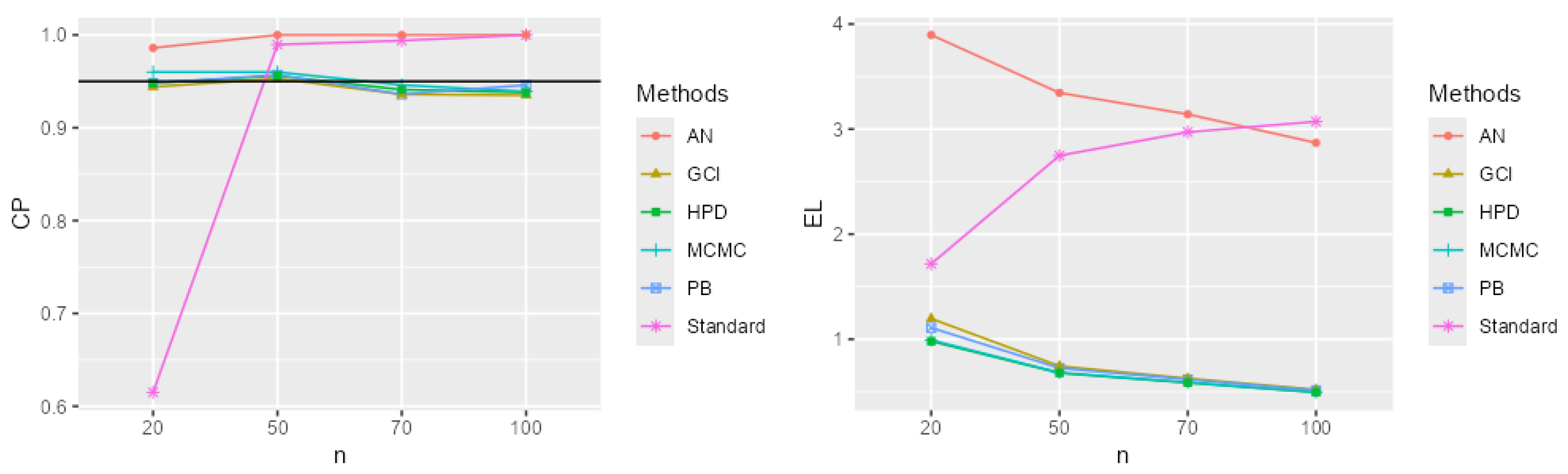
This research compares the efficiency of confidence intervals by evaluating coverage probability (CP) and expected length (EL) using Monte Carlo simulations conducted with the R program version 4.4.1. The main objective of this research is to develop and present a method for constructing confidence intervals for the mean of the zero-inflated two-parameter Rayleigh distribution. Additionally, this study examines the performance of confidence intervals obtained from various approaches, including the percentile bootstrap, generalized confidence interval, standard confidence interval based on maximum likelihood estimation, approximate normal confidence interval using the delta method, Bayesian Markov Chain Monte Carlo, and Bayesian highest posterior density. Sample sizes of n = 20, 50, 70, and 100 were considered. The data were generated from a zero-inflated two-parameter Rayleigh distribution with scale parameters $\lambda$ = 0.2 and 0.5, location parameters $\mu$ = 0.2 and 0.5, and the probability of zeros $\delta$ = 0.2, 0.4, and 0.6. We used M = 1000 replications for the Monte Carlo simulation. For the bootstrap method, each situation involved B = 1000 replications, along with q = 2500 pivotal quantities, and we generated T = 20,000 realizations of Bayesian using Gibbs sampling with a burn-in of C = 5000. The best method was selected based on coverage probability (CP) values that were not lower than the confidence level and the shortest expected length (EL). Specifically, the optimal method was chosen if the CP values were greater than or equal to the 0.95 confidence level and the EL was the shortest.

Evaluate the CP and EL values for the confidence interval of the parameters of the zero-inflated Rayleigh distribution according to Algorithm 7.

Algorithm 7 CP and EL of the confidence intervals for single mean of the zero-inflated two-parameter Rayleigh distribution

1.   Set input the number of process iterations and parameters of distribution $M,B,T,C,n,\mu ,\lambda ,$ and $\delta$. 2.   Generate $x=\left(x_1,\dots x_n\right)$ from $ZITR(\mu ,\lambda ,\delta )$. 3.   Use Algorithm 1 to compute 95% percentile bootstrap confidence interval for the single mean. 4.   Use Algorithm 2 to compute 95% generalized confidence interval for the single mean. 5.   Use Algorithm 3 to compute 95% standard confidence interval using maximum likelihood for the single mean. 6.   Use Algorithm 4 to compute 95% approximate normal for single mean. 7.   Use Algorithm 5 to compute 95% Bayesian MCMC confidence interval for the single mean. 8.   Use Algorithm 6 to compute 95% Bayesian HPD confidence interval for the single mean. 9.   Set $P=1$ if $\left(L\le \mu \le U\right)$, and set $P=0$ if this condition is not satisfied. 10. Find the value of $U-L$. 11. Perform steps 2–8 for M times. 12. Calculate the average of P to assess the coverage probability. 13. Find the average value of the range $U-L$ to assess the expected length.

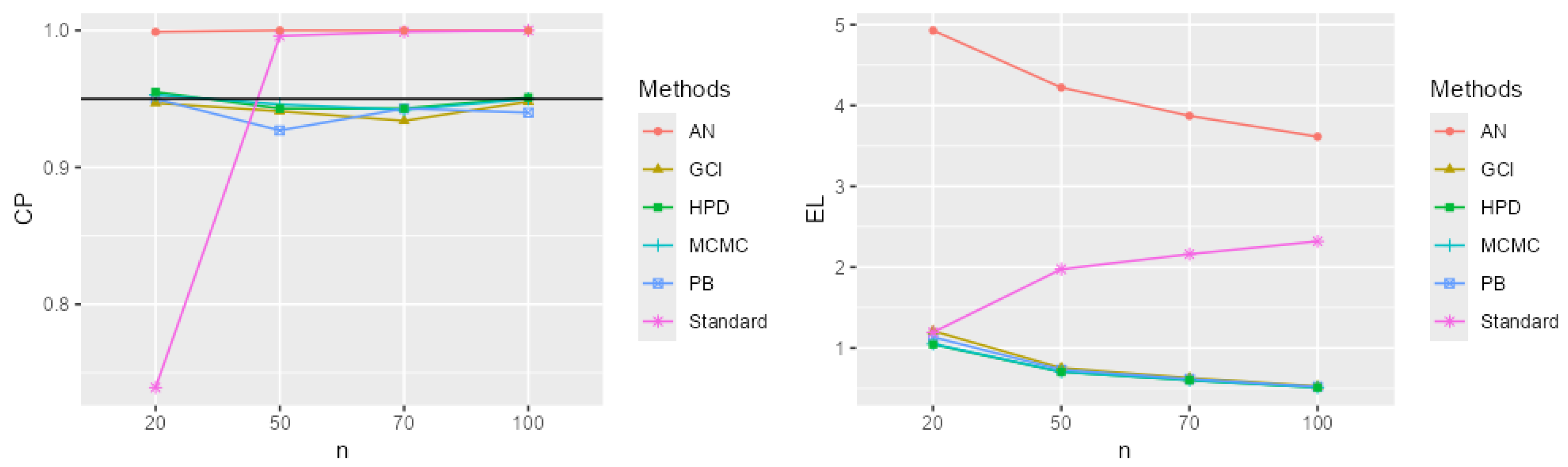
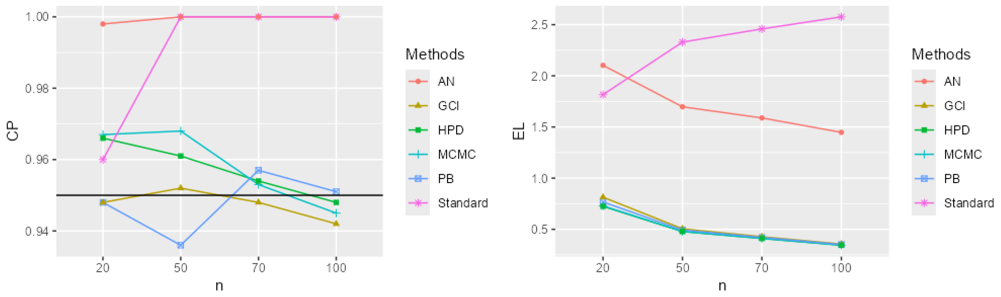
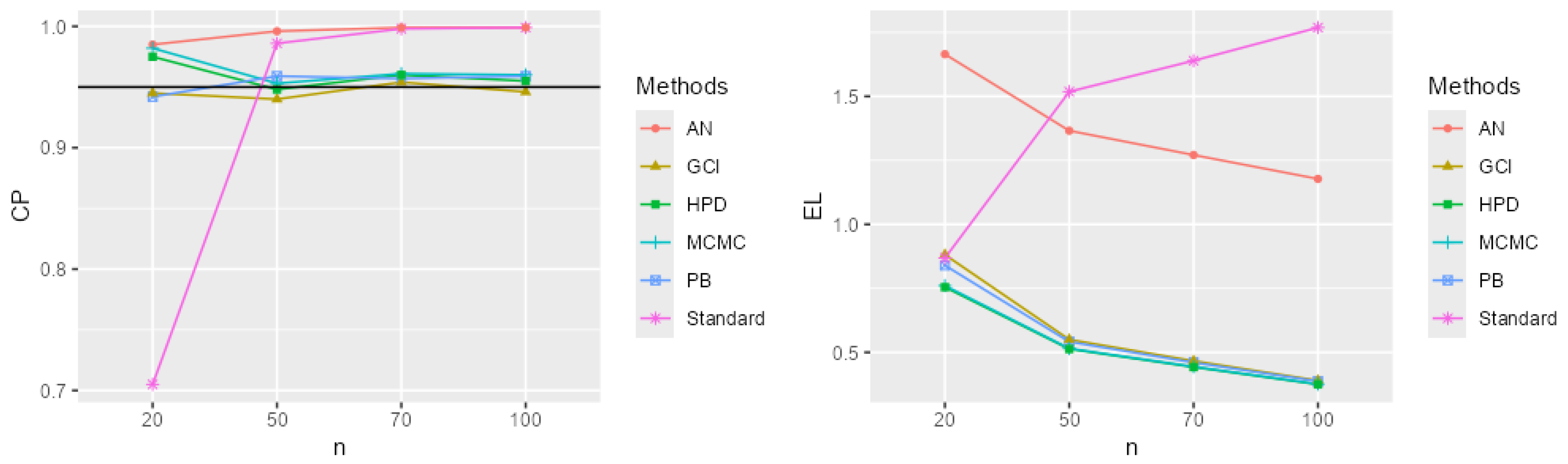
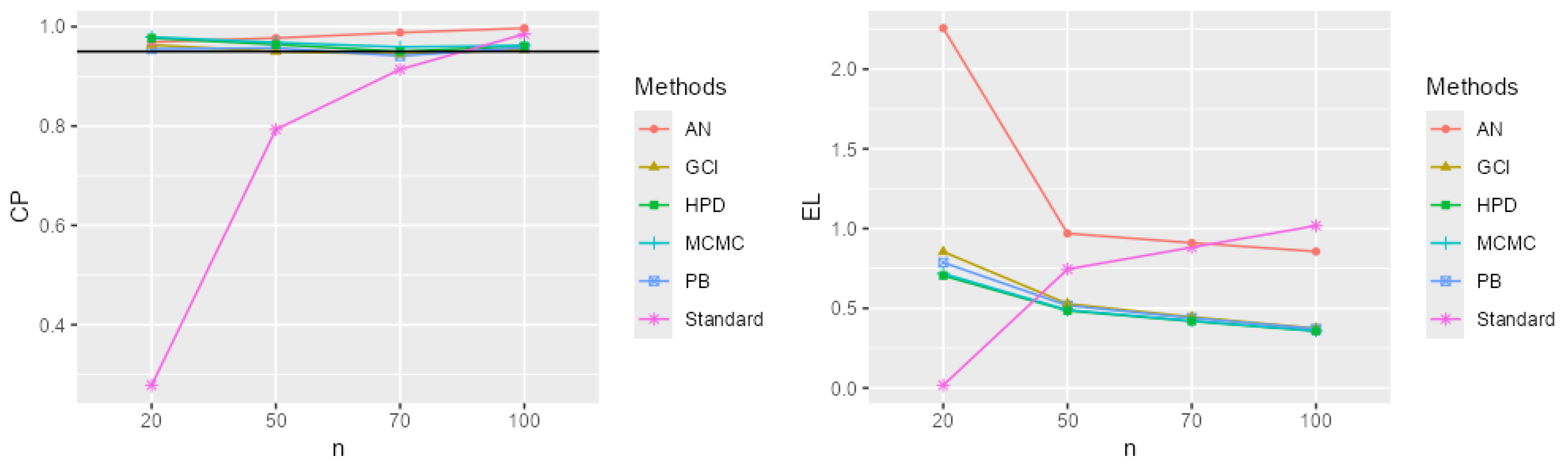
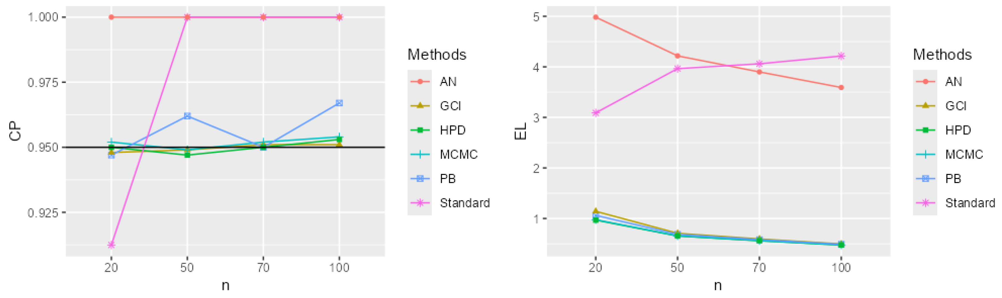
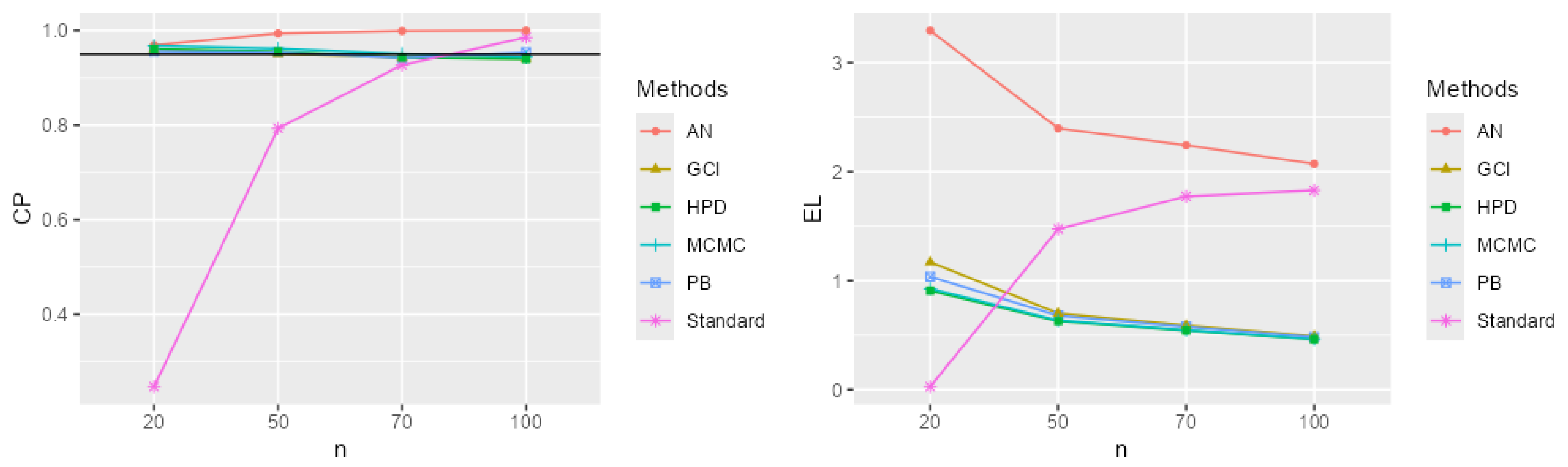
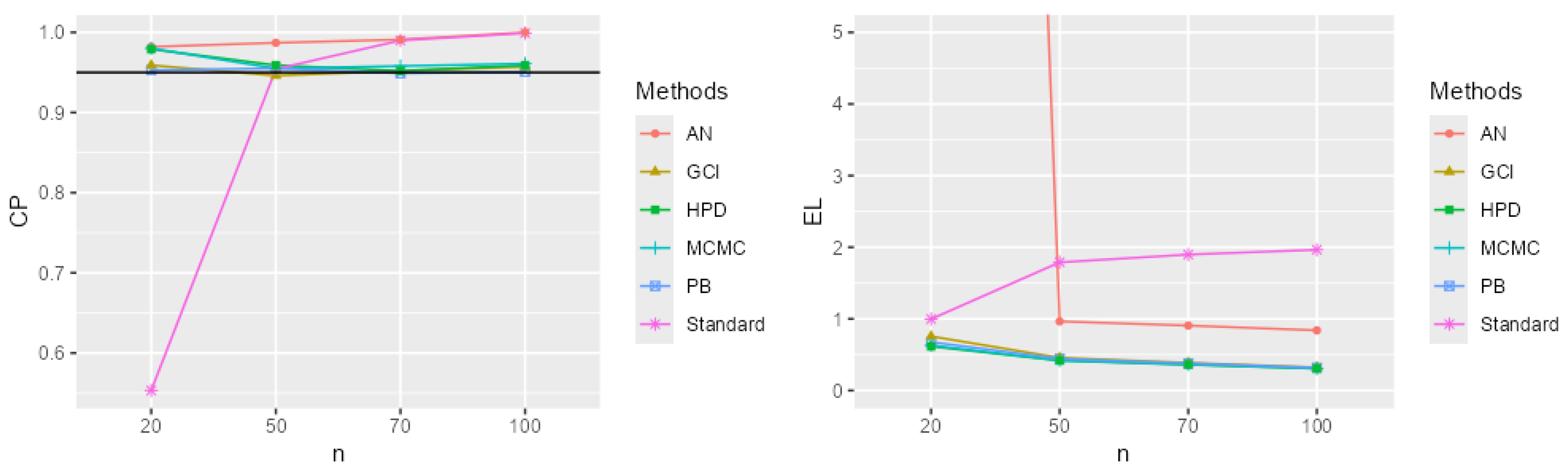
The performance comparison of confidence intervals for the zero-inflated two-parameter Rayleigh distribution, based on simulations using CP and EL values from

Table 1. The coverage probability and expected length for 95% confidence intervals for the single mean of zero-inflated two-parameter Rayleigh distribution when location parameter $\mu =0.2$ and scale parameter $\lambda =0.2,0.5$.

$\mathit{\mu }$	$\mathit{\lambda }$	$\mathit{\delta }$	Coverage Probability
			Sample Size	PB	GCI	Standard	AN	MCMC	HPD
0.2	0.2	0.2	20	0.947	0.948	0.912	1.000	0.952	0.950
				(1.0613)	(1.1424)	(3.0895)	(4.9828)	(0.9762)	(0.9686)
			50	0.962	0.949	1.000	1.000	0.949	0.947
				(0.6865)	(0.7072)	(3.9650)	(4.2171)	(0.6571)	(0.6544)
			70	0.950	0.951	1.000	1.000	0.952	0.950
				(0.5819)	(0.5947)	(4.0601)	(3.8995)	(0.5619)	(0.5599)
			100	0.967	0.951	1.000	1.000	0.954	0.953
				(0.4900)	(0.4965)	(4.2144)	(3.5915)	(0.4766)	(0.4750)
		0.4	20	0.948	0.944	0.615	0.986	0.960	0.948
				(1.1087)	(1.1957)	(1.7170)	(3.8961)	(0.9917)	(0.9806)
			50	0.957	0.953	0.990	1.000	0.960	0.956
				(0.7255)	(0.7438)	(2.7476)	(3.3453)	(0.6817)	(0.6780)
			70	0.936	0.936	0.994	1.000	0.946	0.941
				(0.6166)	(0.6272)	(2.9714)	(3.1413)	(0.5889)	(0.5861)
			100	0.946	0.935	1.000	1.000	0.939	0.938
				(0.5137)	(0.5206)	(3.0712)	(2.8696)	(0.4964)	(0.4943)
		0.6	20	0.956	0.961	0.247	0.969	0.968	0.961
				(1.0357)	(1.1699)	(0.0278)	(3.2929)	(0.9261)	(0.9069)
			50	0.954	0.951	0.793	0.994	0.962	0.956
				(0.6793)	(0.7006)	(1.4736)	(2.3969)	(0.6350)	(0.6282)
			70	0.942	0.943	0.927	0.999	0.951	0.943
				(0.5763)	(0.5887)	(1.7723)	(2.2417)	(0.5472)	(0.5429)
			100	0.954	0.941	0.986	1.000	0.944	0.940
				(0.4834)	(0.4909)	(1.8280)	(2.0708)	(0.4649)	(0.4620)
	0.5	0.2	20	0.955	0.936	0.996	0.999	0.954	0.950
				(0.6829)	(0.7340)	(4.3833)	(2.0454)	(0.6483)	(0.6437)
			50	0.961	0.957	1.000	1.000	0.961	0.958
				(0.4458)	(0.4580)	(4.1724)	(1.6951)	(0.4316)	(0.4300)
			70	0.947	0.957	1.000	1.000	0.961	0.962
				(0.3771)	(0.3854)	(4.3153)	(1.5754)	(0.3687)	(0.3675)
			100	0.950	0.947	1.000	1.000	0.951	0.949
				(0.3177)	(0.3220)	(4.4340)	(1.4593)	(0.3123)	(0.3113)
		0.4	20	0.940	0.960	0.891	0.988	0.976	0.973
				(0.7297)	(0.7795)	(2.2492)	(1.6515)	(0.6673)	(0.6603)
			50	0.960	0.948	0.999	0.999	0.957	0.957
				(0.4731)	(0.4842)	(3.0704)	(1.3466)	(0.4508)	(0.4485)
			70	0.961	0.940	0.999	0.999	0.948	0.949
				(0.4020)	(0.4079)	(3.0445)	(1.2497)	(0.3874)	(0.3857)
			100	0.960	0.955	1.000	1.000	0.960	0.959
				(0.3374)	(0.3416)	(3.1435)	(1.1620)	(0.3287)	(0.3274)
		0.6	20	0.953	0.959	0.553	0.982	0.980	0.979
				(0.6761)	(0.7563)	(0.9973)	(47.5421)	(0.6291)	(0.6160)
			50	0.955	0.946	0.954	0.987	0.955	0.959
				(0.4442)	(0.4573)	(1.7898)	(0.9649)	(0.4219)	(0.4176)
			70	0.949	0.952	0.990	0.991	0.958	0.952
				(0.3792)	(0.3865)	(1.8977)	(0.9065)	(0.3638)	(0.3610)
			100	0.951	0.957	0.999	1.000	0.961	0.959
				(0.3184)	(0.3220)	(1.9650)	(0.8398)	(0.3082)	(0.3063)

The bold represents the values that provide the shortest expected length when coverage probability is greater than or equal to the confidence level.

and

Table 2. The coverage probability and expected length for 95% confidence intervals for the single mean of zero-Inflated two-parameter Rayleigh distribution when location parameter $\mu =0.5$ and scale parameter $\lambda =0.2,0.5$.

$\mathit{\mu }$	$\mathit{\lambda }$	$\mathit{\delta }$	Coverage Probability
			Sample Size	PB	GCI	Standard	AN	MCMC	HPD
0.5	0.2	0.2	20	0.950	0.947	0.739	0.999	0.953	0.955
				(1.1351)	(1.2116)	(1.1942)	(4.9282)	(1.0506)	(1.0443)
			50	0.927	0.941	0.996	1.000	0.946	0.943
				(0.7321)	(0.7531)	(1.9751)	(4.2223)	(0.7069)	(0.7046)
			70	0.943	0.934	0.999	1.000	0.942	0.943
				(0.6171)	(0.6302)	(2.1609)	(3.8720)	(0.6033)	(0.6014)
			100	0.940	0.948	1.000	1.000	0.950	0.951
				(0.5209)	(0.5285)	(2.3193)	(3.6142)	(0.5129)	(0.5114)
		0.4	20	0.952	0.954	0.343	0.991	0.968	0.965
				(1.2227)	(1.2952)	(0.3320)	(3.9528)	(1.0840)	(1.0743)
			50	0.943	0.952	0.878	1.000	0.959	0.958
				(0.7887)	(0.8059)	(1.1292)	(3.3220)	(0.7448)	(0.7414)
			70	0.948	0.949	0.970	1.000	0.957	0.955
				(0.6737)	(0.6825)	(1.3055)	(3.1409)	(0.6453)	(0.6428)
			100	0.938	0.953	0.998	1.000	0.954	0.954
				(0.5620)	(0.5674)	(1.4985)	(2.8860)	(0.5455)	(0.5436)
		0.6	20	0.953	0.966	0.273	0.966	0.984	0.981
				(0.7879)	(0.8559)	(0.0088)	(2515.8700)	(0.7201)	(0.7075)
			50	0.961	0.947	0.504	0.989	0.961	0.950
				(0.7479)	(0.7667)	(0.4056)	(2.3583)	(0.6979)	(0.6916)
			70	0.957	0.949	0.742	0.997	0.963	0.956
				(0.6362)	(0.6478)	(0.6132)	(2.2573)	(0.6057)	(0.6016)
			100	0.958	0.947	0.900	1.000	0.951	0.947
				(0.5357)	(0.5422)	(0.7632)	(2.0905)	(0.5154)	(0.5126)
	0.5	0.2	20	0.948	0.948	0.960	0.998	0.967	0.966
				(0.7670)	(0.8139)	(1.8159)	(2.1024)	(0.7283)	(0.7247)
			50	0.936	0.952	1.000	1.000	0.968	0.961
				(0.4931)	(0.5046)	(2.3294)	(1.6972)	(0.4793)	(0.4780)
			70	0.957	0.948	1.000	1.000	0.953	0.954
				(0.4201)	(0.4274)	(2.4583)	(1.5883)	(0.4112)	(0.4101)
			100	0.951	0.942	1.000	1.000	0.945	0.948
				(0.3514)	(0.3557)	(2.5764)	(1.4473)	(0.3452)	(0.3442)
		0.4	20	0.942	0.945	0.705	0.985	0.982	0.975
				(0.8398)	(0.8814)	(0.8684)	(1.6648)	(0.7607)	(0.7546)
			50	0.959	0.940	0.986	0.996	0.953	0.948
				(0.5415)	(0.5499)	(1.5184)	(1.3659)	(0.5150)	(0.5131)
			70	0.957	0.954	0.998	0.999	0.961	0.960
				(0.4604)	(0.4666)	(1.6394)	(1.2711)	(0.4439)	(0.4424)
			100	0.959	0.946	0.999	0.999	0.960	0.955
				(0.3870)	(0.3899)	(1.7688)	(1.1777)	(0.3760)	(0.3749)
		0.6	20	0.955	0.963	0.278	0.969	0.979	0.977
				(0.7868)	(0.8547)	(0.0174)	(2.2573)	(0.7175)	(0.7052)
			50	0.957	0.950	0.793	0.977	0.968	0.964
				(0.5174)	(0.5279)	(0.7450)	(0.9693)	(0.4891)	(0.4850)
			70	0.941	0.945	0.914	0.988	0.959	0.950
				(0.4390)	(0.4454)	(0.8821)	(0.9104)	(0.4214)	(0.4188)
			100	0.958	0.954	0.985	0.997	0.962	0.961
				(0.3712)	(0.3739)	(1.0177)	(0.8563)	(0.3586)	(0.3568)

The bold represents the values that provide the shortest expected length when coverage probability is greater than or equal to the confidence level.

and Figure 2, Figure 3, Figure 4, Figure 5, Figure 6, Figure 7, Figure 8, Figure 9, Figure 10, Figure 11, Figure 12 and Figure 13, focuses on the confidence intervals of the single mean, with scale parameters $\lambda =0.2,0.5$ and location parameter $\mu =0.2,0.5$. The standard confidence interval based on maximum likelihood provides coverage probabilities lower than the nominal confidence level and exhibits a larger expected length compared to other methods, especially for small sample sizes. The approximate normal method using the delta method yields higher CP values than the standard method but also results in greater expected lengths. The expected length generally decreases as the sample size increases across most methods. The simulation results across various scenarios indicate that the Bayesian method outperforms the others in estimating the single mean when evaluated based on CP and EL. Additionally, the Bayesian HPD interval offers the shortest credible interval length.

4. Application

The total death rate from COVID-19 plays a crucial role in understanding the overall impact of the pandemic on public health. This information enables governments and health authorities to assess the severity of the outbreak and evaluate the effectiveness of the implemented control measures. Moreover, it is valuable for planning and allocating medical resources appropriately based on the situation. Additionally, it helps raise public awareness about the importance of disease prevention and encourages greater compliance with recommendations from government agencies and health organizations. COVID-19 total death data for Singapore in October 2022 were compiled by the World Health Organization (WHO) and are accessible at https://covid19.who.int/WHO-COVID-19-globaldata.csv (last accessed on 28 June 2023). The n = 31 was as follows: 2, 1, 2, 2, 0, 1, 0, 4, 0, 3, 2, 2, 3, 0, 2, 3, 2, 5, 3, 5, 0, 1, 2, 1, 3, 2, 2, 0, 4, 2, 4. The zero observations in the dataset were modeled using a binomial distribution, while the positive data were analyzed using the model with the minimum Akaike information criterion (AIC) and minimum Bayesian information criterion (BIC), as reported in

Table 3. AIC values of total death dataset for fitting distribution.

Distribution	Two-Parameter Rayleigh	Normal	Weibull	Lognormal	Exponential	Gamma
AIC	77.3115	81.3052	78.8253	77.9169	97.213	77.643

The bold represents the distribution values that result in the minimum AIC.

and

Table 4. BIC values of total death dataset for fitting distribution.

Distribution	Two-Parameter Rayleigh	Normal	Weibull	Lognormal	Exponential	Gamma
BIC	79.74922	83.74298	81.26306	80.35464	99.43182	80.08071

The bold represents the distribution values that result in the minimum BIC.

. The parameter estimates for the dataset are statistically summarized as follows: $n=31,\widehat{\delta }=0.1936,\widehat{\lambda }=0.1876$, and $\widehat{\mu }=0.5$. The confidence interval for the single mean of total COVID-19 deaths in Singapore is reported in

Table 5. The confidence interval for single mean of total death for COVID-19 in Singapore during October 2022.

CI	Percentile		GCI		STD		AN		MCMC		HPD
	Lower	Upper	Lower	Upper	Lower	Upper	Lower	Upper	Lower	Upper	Lower	Upper
$\psi$	1.5224	2.5762	1.5858	2.5833	1.1280	2.7929	0.3157	3.8068	1.3599	2.2742	1.3602	2.2742
	(1.0538)		(0.9975)		(1.6649)		(3.4911)		(0.9142)		(0.9139)

The values in () represent the width of the confidence intervals constructed from the actual data.

.

The results are shown in Table 5. The confidence interval for total deaths from COVID-19 in Singapore is not recommended using the standard confidence interval based on maximum likelihood or the approximate normal method derived from the delta method. The simulation results indicate that when the sample size n is small, the standard confidence interval often results in a coverage probability that fails to include the true mean. Moreover, as the value of $\delta$ increases, the mean estimator fails to capture the true mean of the target distribution, and the resulting confidence interval tends to be wider than those obtained from other methods. Similarly, for the approximate normal (AN) method, although the confidence interval tends to cover the parameter and becomes narrower as n increases, it still produces wider intervals than other methods when n is small. Therefore, we recommend the percentile bootstrap method, the GCI method, the Bayesian MCMC method, and the Bayesian HPD method as these approaches provide confidence intervals that adequately cover the mean parameter. Among them, the Bayesian HPD method is concluded to be the most effective as it produces the narrowest expected length for the confidence interval of the mean.

5. Discussion

Previous studies on constructing confidence intervals and Bayesian estimation have often shown that Bayesian methods yield the most effective results. In this research, Bayesian approaches were employed to construct confidence intervals for the single mean of the zero-inflated Rayleigh distribution. Specifically, the scale parameter was modeled using a gamma prior, while the location parameter was modeled using a uniform prior. The results indicated that Bayesian credible intervals performed well in nearly all scenarios, consistently achieving coverage probabilities close to the specified confidence level. This consistent and stable performance suggests that the Markov chains have likely converged satisfactorily. Furthermore, the Bayesian highest posterior density (HPD) intervals demonstrated superior performance compared to the Bayesian MCMC intervals in several cases. For example, when the parameters were $\mu =0.2$, $\lambda =0.2$, and $\delta =0.2$, the HPD method outperformed the MCMC method for sample sizes of 20, 70, and 100. Similarly, for $\lambda =0.2$, $\mu =0.5$, and $\delta =0.4$, the HPD method showed better performance for sample sizes of 20, 50, and 100. When the parameters were $\lambda =0.5$, $\mu =0.2$, and $\delta =0.6$, the HPD method again outperformed the MCMC method for sample sizes of 20, 50, and 70. Moreover, in several other scenarios not explicitly mentioned, the HPD method consistently yielded better results. In particular, when the parameters were $\lambda =0.2$, $\mu =0.5$, and $\delta =0.6$, or $\lambda =0.5$, $\mu =0.5$, and $\delta =0.6$, the HPD method outperformed the MCMC method across all sample sizes.

6. Conclusions

This paper presents confidence intervals for the single mean of a zero-inflated two-parameter Rayleigh distribution with unknown location and scale parameters. Various methods for estimating the single mean were considered, including the percentile bootstrap, generalized confidence interval (GCI), standard confidence interval based on maximum likelihood, and the approximate normal method using the delta method, as well as the Bayesian MCMC and Bayesian HPD methods. The performance of these methods was evaluated based on coverage probability and expected length through a simulation study. The results revealed that the percentile bootstrap, GCI, Bayesian MCMC, and Bayesian HPD methods produced coverage probabilities that exceeded the specified confidence level. However, the confidence intervals constructed using the standard maximum likelihood and delta method approaches proved unsuitable for the sample size under consideration as they resulted in excessively wide expected lengths, despite covering the parameter of interest. In certain scenarios, the Bayesian highest posterior density (HPD) method outperformed other approaches by delivering coverage probabilities (CPs) that reliably encompassed the parameter of interest while also producing shorter expected lengths (ELs). Nonetheless, in instances where coverage was inadequate, the Bayesian MCMC method exhibited the second-best performance.

In the application, we analyzed the total number of COVID-19-related deaths in Singapore during October 2022. Based on the simulation results, the Bayesian credible interval methods outperformed the other approaches, with the Bayesian HPD method demonstrating the best performance in constructing the confidence interval for the single mean of the zero-inflated two-parameter Rayleigh distribution. Therefore, the Bayesian HPD method is recommended for constructing the confidence interval for the total number of COVID-19 deaths in Singapore during this period.