Symmetry-Inspired Friction Compensation and GPI Observer-Based Nonlinear Predictive Control for Enhanced Speed Regulation in IPMSM Servo Systems

Abstract

In integrated permanent magnet synchronous motors (IPMSMs) coupled with mechanical devices such as ball screws and reducers, complex nonlinear friction characteristics often arise, leading to asymmetrical distortions such as position “flat-top” and speed “ramp-up”. These phenomena significantly degrade the system’s positioning accuracy. To address this issue, this paper introduces a symmetry-inspired nonlinear predictive speed control approach based on the Stribeck piecewise linearized friction compensation and a generalized proportional integral (GPI) observer. The proposed method leverages the inherent symmetry in the Stribeck friction model to describe the nonlinear behavior, employing online piecewise linearization via the least squares method. A GPI observer was designed to estimate the lumped disturbance, including time-varying components in the speed dynamics, friction model deviations, and external loads. By incorporating these estimates, a nonlinear predictive controller was developed, employing a quadratic cost function to derive the optimal control law. The experimental results demonstrate that, compared to traditional integral NPC and PI controllers, the proposed method effectively restores system symmetry by eliminating the “flat-top” and “ramp-up” distortions while maintaining computational efficiency.

1. Introduction

The application of integrated permanent magnet synchronous motors (IPMSMs) is no longer limited to traditional fields such as textiles and welding; it is increasingly being used in high-end areas such as precision instruments and aerospace electromechanical actuators [1,2,3,4,5]. These high-tech fields often have extremely high requirements for the speed control accuracy of IPMSM electromechanical servo systems [6,7], and any errors in control accuracy are often intolerable in these advanced technology sectors [8,9]. Whether in precision instruments or electromechanical actuators, basic mechanical components, such as ball screws, are commonly used in devices aimed at positioning [10,11]. Ball screws can effectively convert the rotation of the electromechanical servo system into linear motion [12], offering advantages such as high transmission efficiency, high transmission accuracy, and long service life [13].

IPMSMs are typically used in conjunction with mechanical devices such as ball screws and reducers under a weak magnetic control framework [14,15,16]. However, such assemblies can lead to complex nonlinear friction issues [17], resulting in significant “flexibility” in the electromechanical servo system [18], which, ultimately, greatly reduces position control accuracy [19]. Many studies have shown that in this type of flexible servo system, position errors often occur in the zero-speed reversal region during reciprocating motion. In this region, there exist the phenomena of a “flat-top” position and a “ramp-up” speed, which manifest as a severe distortion similar to “loss of response” in position and speed tracking [20,21,22]. The cause of these phenomena is the nonlinear friction in flexible electromechanical servo systems, which is particularly strong at low speeds, thereby significantly affecting the repeatability of positioning accuracy [23]. If the design of the speed loop controller can be improved to enable it to compensate for and suppress nonlinear friction, it would greatly enhance the positioning accuracy of such precision machinery without increasing economic costs [24,25,26].

Many engineers and scholars have proposed different methods to address the nonlinear friction problem in IPMSM electromechanical servo systems. Reference [27] proposed a friction force identification and compensation method based on a matching-following algorithm. This method does not rely on a friction model but compensates for the friction dynamics through orthogonal polynomial approximation. The method offers high compensation accuracy, but due to the need for real-time online calculation and the large computational load, it is still in the offline simulation stage. Reference [28] proposed a sliding mode control strategy that leverages the LuGre friction model in conjunction with genetic algorithm-based identification techniques. This method improves the accuracy of friction compensation due to the high order of the friction model and the high precision of the identification algorithm. However, as it requires offline identification of the LuGre friction model using genetic algorithms and then uses the identified model to improve sliding mode control, the method’s online performance is still not sufficient, lacking real-time capability and adaptability for practical applications. Reference [29] introduced an adaptive control approach that incorporates the Stribeck friction model. In this method, the Stribeck friction model is approximated by piecewise linearization, and the Stribeck linearized model is identified online using a least squares method, which can be used in real time and is computationally efficient. The adaptive control improves the accuracy of friction compensation, and the entire algorithm works in real time and is easy to implement.

Based on a comprehensive mechanism modeling and analysis of the IPMSM electromechanical servo system, this paper proposes a nonlinear predictive speed control (NPC + GPIO + FRIC) based on Stribeck piecewise linearized friction compensation and a GPI observer. Initially, the Stribeck friction model, capable of thoroughly reflecting the nonlinear friction properties of flexible electromechanical servo systems, was selected, considering real-time efficiency and feasibility while ensuring model accuracy. The Stribeck friction model undergoes piecewise linearization using a least squares matrix algorithm with reduced online computation. Subsequently, using the identified friction model, the terms associated with speed dynamics, deviations in the model, and load torques (excluding friction) are collectively treated as a lumped disturbance. A GPI observer is employed to estimate the lumped disturbance. GPIO was initially introduced in [30] and further studied in [31,32,33], demonstrating its effectiveness in estimating different disturbance sources. Building on the lumped disturbance estimation, a nonlinear predictive control framework was further developed. Nonlinear predictive control (NPC), an iteration of Model Predictive Control (MPC), facilitates optimized control strategies for nonlinear control systems.

The major contributions of this paper include three aspects: (1) Taking nonlinear friction into account, the accurate mathematical model of the IPMSM electromechanical servo system is reconstructed. This achievement encompasses Stribeck friction modeling, linearization, and identification while ensuring real-time capability, versatility, and minimal computational load. (2) The time-varying parameters of the motor and the deviations of the identified friction model are treated as a type of lumped disturbance. A GPIO-based compensation method is designed to mitigate this disturbance, thereby ensuring robustness in speed control. (3) A nonlinear predictive control strategy is formulated, incorporating symmetry-inspired friction model identification and disturbance compensation, with the aim of enhancing speed closed-loop tracking performance.

After conducting a stability analysis of the proposed approach, comprehensive comparative experiments were performed on an IPMSM servo system platform to assess the practical feasibility and effectiveness of the suggested control strategy. The experimental outcomes reveal that the proposed speed control method delivers robust performance, effectively managing parameter variations and nonlinear friction disturbances. Compared with the integral NPC scheme and traditional PI control, it basically eliminates the position “flat-top” phenomenon and speed “ramp-up” phenomenon in position control mode without significantly increasing the online computational workload.

2. Preliminaries

2.1. Basic Dynamic Model of IPMSM

To establish a more effective mathematical model of IPMSMs, the following assumptions need to be made before modeling:

(1)

Ignore the stator hysteresis and eddy current losses of the IPMSM;

(2)

Assume that the magnetic circuit of the IPMSM can be analyzed according to the superposition theorem;

(3)

The excitation magnetic field and magnetomotive force of IPMSM follow a strictly sinusoidal distribution across the air gap, and higher-order harmonics are neglected;

(4)

During steady-state operation of the motor, the electromotive force of the three-phase symmetrical windings is in the form of a standard undistorted sine, with a mutual phase difference of 120 electrical degrees;

(5)

Ignore the inverter dead-time effect;

(6)

Ignore the backlash effect of the IPMSM.

Based on the above assumptions, through a series of mathematical derivations using the commonly applied Park transformation, inverse Park transformation, and Clarke transformation in the field of servo control, we can obtain the nominal speed mathematical model and the d- and q-axes of the dynamic nominal current mathematical models of the IPMSM as [32]

$$\begin{array}{cc}\hfill & {\displaystyle \frac{d\omega }{dt}}={\displaystyle \frac{1}{J}}\left\{\left[n_p\left(L_d-L_q\right)i_d+n_p{\psi }_f\right]i_q-B\omega -T_f\right\},\hfill \\ \hfill & {\displaystyle \frac{d{i}_d}{dt}}={\displaystyle \frac{1}{L_d}}(-R_s{i}_d+u_d+u_d^{coupling}),\hfill \\ \hfill & {\displaystyle \frac{d{i}_q}{dt}}={\displaystyle \frac{1}{L_q}}(-R_s{i}_q+u_q+u_q^{coupling}),\hfill \end{array}$$

(1)

where J is the moment of inertia, $n_p$ is the number of pole pairs, ${\psi }_f$ is the rotor flux linkage, $\omega$ is the rotor angular speed, $T_f$ is the friction torque, $R_s$ is the nominal value of the stator resistance, $L_d$ and $L_q$ are respectively the d- and q-axes stator inductances, $i_d$ and $i_q$, are, respectively, the d and q axes of the stator currents, B is the friction coefficient, $u_d$ and $u_q$ are, respectively, the d and q axes of the stator voltages, and $u_d^{coupling}$ and $u_q^{coupling}$ are, respectively, the d and q axes of the cross-coupling terms. The cross-coupling terms are given by

$$\begin{array}{cc}\hfill & u_d^{coupling}=n_p\omega L_q{i}_q,\hfill \\ \hfill & u_q^{coupling}=-n_p\omega L_d{i}_d-n_p\omega {\psi }_f.\hfill \end{array}$$

(2)

Remark 1 

(Nonlinear cross-coupling terms). In Equation (2), the d-axis coupling term $n_p\omega L_q{i}_q$ is related to the q-axis stator current $i_q$, and the q-axis coupling term $-n_p\omega L_d{i}_d-n_p\omega {\psi }_f$ is related to the d-axis stator current $i_d$, so they are together called cross-coupling terms. Those multiply-form nonlinear cross-coupling terms are effectively handled by employing the methods presented in [32].

Furthermore, considering the motor parameter variations, each motor parameter can be expressed as the sum of its nominal value and change, given by

$$\begin{array}{cc}\hfill & J=J_0+\Delta J,\hfill \\ \hfill & R_s=R_{s0}+\Delta R_s,\hfill \\ \hfill & L_d=L_{d0}+\Delta L_d,\hfill \\ \hfill & L_q=L_{q0}+\Delta L_q,\hfill \\ \hfill & {\psi }_f={\psi }_{f0}+\Delta {\psi }_f,\hfill \\ \hfill & B=B_0+\Delta B,\hfill \end{array}$$

(3)

where $J_0$ and $\Delta J$ are, respectively, the moment of inertia of the electromechanical servo system body and its load, $R_{s0}$ and $\Delta R_s$ are, respectively, the nominal value and change in stator resistance, $L_{d0}$ and $\Delta L_d$ are, respectively, the nominal value and change in the d-axis stator inductance, $L_{q0}$ and $\Delta L_q$ are, respectively, the nominal value and change in the q-axis stator inductance, ${\psi }_{f0}$ and $\Delta {\psi }_f$ are, respectively, the nominal value and change in the rotor flux linkage, and $B_0$ and $\Delta B$ are, respectively, the nominal value and change in the friction coefficient. Substituting Equation (3) into Equation (1), the dynamic model of the IPMSM from Equation (1) can be rewritten as

$$\begin{array}{cc}\hfill & {\displaystyle \frac{d\omega }{dt}}={\displaystyle \frac{1}{J_0}}\left\{\left[n_p\left(L_{d0}-L_{q0}\right)i_d+n_P{\psi }_{f0}\right]i_q-B_0\omega -p_{\omega }-T_f\right\},\hfill \\ \hfill & {\displaystyle \frac{d{i}_d}{dt}}={\displaystyle \frac{1}{L_{d0}}}(u_d-R_{s0}{i}_d+n_p\omega L_{q0}{i}_q+p_d),\hfill \\ \hfill & {\displaystyle \frac{d{i}_q}{dt}}={\displaystyle \frac{1}{L_{q0}}}(u_q-R_{s0}{i}_q-n_p\omega L_{d0}{i}_d-n_p\omega {\psi }_{f0}+p_q),\hfill \end{array}$$

(4)

where $p_{\omega }$ is the lumped disturbance in the speed dynamic, given by

$$\begin{array}{c}\hfill p_{\omega }={\displaystyle \frac{1}{J_0}}\left\{\left[n_p\left(\Delta L_{d0}-\Delta L_{q0}\right)i_d+n_P\Delta {\psi }_{f0}\right]i_q-\Delta B\omega -T_{\mathrm{L}}-\Delta J{\displaystyle \frac{d\omega }{dt}}\right\},\end{array}$$

(5)

and $p_d$ and $p_d$ are, respectively, the d and q axes of the time-varying voltages terms, given by

$$\begin{array}{cc}\hfill & p_d=-\Delta R_s{i}_d+n_p\omega \Delta L_q{i}_q-\Delta L_d{\displaystyle \frac{d{i}_d}{dt}},\hfill \\ \hfill & p_q=-\Delta R_s{i}_q-n_p\omega \Delta L_d{i}_d-n_p\omega \Delta {\psi }_f-\Delta L_q{\displaystyle \frac{d{i}_q}{dt}}.\hfill \end{array}$$

(6)

Remark 2. 

The terms $p_d$ and $p_d$ caused by the motor parameter variations are time-varying, and, moreover, they grow greater from the CT region to the FW region. Hence, they also need major consideration in the current controller design.

Following the cascade control framework of electromechanical servo systems and the design principle of the IPMSM field-weakening control method [32], the $i_q$ in Equation (6) is considered the control law for velocity dynamics, where the designed velocity control law acts as the q-axis of the reference current $i_q^{*}$. The d-axis of the reference current $i_d^{*}$ is derived from a field-weakening algorithm. Define the coefficient of $i_q$ in Equation (6) as the generalized torque coefficient ${\overline{K}}_t$, that is

$$\begin{array}{c}\hfill {\overline{K}}_t=n_P\left(L_{d0}-L_{q0}\right)i_d+n_P{\psi }_{f0},\end{array}$$

(7)

and it is noted that since ${\overline{K}}_t$ is related to $i_d$, it is time-varying.

Remark 3 

(Motor parameters variations). It can be observed from the expression for $p_{\omega }$ in Equation (5) that the first term ${\displaystyle \frac{1}{J_0}}\left[n_P\left(\Delta L_{d0}-\Delta L_{q0}\right)i_d+n_P\Delta {\psi }_{f0}\right]i_q$ represents the time-varying reduced terms of parameters $L_d$, $L_q$, and ${\psi }_f$, indicating the impact of perturbations in these three parameters on the speed dynamics; the second term ${\displaystyle \frac{1}{J_0}}\Delta B\omega$ represents the time-varying reduced term for the parameter B, illustrating the influence of the perturbation in the body friction coefficient on the speed dynamics; the second term ${\displaystyle \frac{1}{J_0}}{T}_L$ represents the time-varying reduced term for the parameter B, illustrating the influence of the perturbation in the body friction coefficient on the speed dynamics; the third term ${\displaystyle \frac{1}{J_0}}{T}_L$ indicates the effect of the load torque on the speed dynamics; the fourth term $\Delta J{\displaystyle \frac{d\omega }{dt}}$ is the time-varying reduced term for parameter J, representing the influence of inertia perturbation on the speed dynamics.

Remark 4 

(Various load torques). It is noted that the characteristic of the third term ${\displaystyle \frac{1}{J_0}}{T}_L$ in Equation (5) represents the portion of the load torque consumed by driving loads. In this paper, the load torque $T_L$ and the friction torque $T_f$ are considered separately. In practical applications, the magnitude of the driven load varies, making the handling of this term a critical consideration in the design of the speed loop controller.

Remark 5 

(Nonlinear friction torque). Noting that $T_f$ in Equation (4) represents the friction torque, it signifies the nonlinear friction challenge encountered by IPMSMs in applications involving flexible mechanical components such as ball screws and belt pulleys. The nonlinear friction challenge is manifested by the strong nonlinearity of the friction torque, which differs across various flexible load scenarios. If the nonlinear friction torque is not well handled, it would lead to a reduction in the precision of the speed controller. This precision reduction is particularly severe in the negative velocity reversal region, where a “flat-top” position phenomenon and a “ramp-up” speed phenomenon occur. These phenomena manifest as severe distortion, resembling a “loss of response” in position and speed tracking. In this paper, this challenge will be addressed through the design of a friction compensation speed controller. It is worth noting that the proper handling of nonlinear frictional torque is critical for electromechanical servo systems, as it not only relates to control accuracy but also to system reliability. The improper handling of frictional torque can lead to malfunctions in the electromechanical system. Approaches are provided to analyze and address reliability issues and such fault problems from both the perspectives of the functions in reference [34] and structure in reference [35].

2.2. Generalized IPMSM Object Based on the Cascade Flux-Weakening Control Framework

A cascade framework is usually used for motor control in industrial applications. In this framework, the speed loop control and current loop control can be designed separately. For the sake of convenience, here, we treat the current closed-loop control of the IPMSM as a whole, based on the cited reference, while designing the speed loop controller independently. Figure 1 shows this framework, where the generalized IPMSM object represents an integrated system encompassing the current loop controller, the IPMSM, and the power electronics units, and the speed is regulated by a speed controller designed in this study. In Figure 1, ${\omega }^{*}$ represents the reference speed, and $i_q^{*}$ represents the reference q-axis current.

3. Controller Design

Here, considering the motor parameter variations, the various load torques, and the nonlinear friction torque, a novel nonlinear predictive control based on friction compensation was designed to minimize the deviation between the feedback speed and the reference speed in the IPMSM electromechanical servo system.

3.1. Symmetry-Inspired Stribeck Segmented Linearized Friction Model Identification

The Stribeck friction characteristic curve of the electromechanical servo system is shown in Figure 2, and the expression for the friction torque is [17]

$$\begin{array}{c}\hfill T_f=\left[T_c+\left(T_s-T_c\right)e^{-{\left(\omega /{\omega }_s\right)}^2}\right]sgn\left(\omega \right)+B_s\omega .\end{array}$$

(8)

Within the ultra-low-speed range ${\omega }_s^{-}<\omega <{\omega }_s^{+}$, the friction torque demonstrates significant nonlinearity, decreasing with rising speed. In the adjacent speed ranges, the friction torque shows relatively better linearity and increases with higher speed. Directly employing the Stribeck friction model shown in Equation (8) as the fitting function, given its complexity relative to polynomials, necessitates the use of genetic algorithms or simulated annealing algorithms for identification. This yields a highly precise Stribeck friction model for electromechanical servo systems, but the online computational burden is too heavy for the DSP chip of such systems. Consequently, it is essential to explore methods to reduce the complexity of the fitting algorithm while ensuring that the control performance of the speed controller based on friction compensation is minimally affected.

The Stribeck friction characteristic curve shown in Figure 2 reveals that both when the motor is in reverse rotation ($\omega <0$) and forward rotation ($\omega >0$), the absolute value of the friction torque reaches a minimum. These two speed points are denoted as ${\omega }_s^{-}$ (reverse rotation) and ${\omega }_s^{+}$ (forward rotation), respectively.

By dividing the Stribeck friction model into four speed ranges $\omega \le {\omega }_s^{-}$, ${\omega }_s^{-}<\omega <0$, $0\le \omega <{\omega }_s^{+}$, and $\omega \ge {\omega }_s^{+}$, and using linear fitting functions in each range to approximate the Stribeck characteristic curve, it can be seen that the resulting piecewise linearized friction model remains quite close to the Stribeck characteristics. The Stribeck friction characteristics exhibit higher linearity in the speed ranges $\omega \le {\omega }_s^{-}$ and $\omega \ge {\omega }_s^{+}$, while the linearity is relatively poor in the ultra-low speed ranges of ${\omega }_s^{-}<\omega <0$ and $0\le \omega <{\omega }_s^{+}$. Therefore, the piecewise linearization method introduces some deviation in the friction model in the ultra-low speed ranges. In the design of the speed controller in this study, targeted treatment was applied to this friction model deviation.

The SRIBECK friction model can be written in the form of four linearized segments [17], given by

$$\begin{array}{c}\hfill {\widehat{T}}_f=\left\{\begin{array}{c}{\alpha }_0+{\alpha }_1\omega ,\omega \le {\omega }_s^{-}\hfill \\ {\beta }_0+{\beta }_1\omega ,{\omega }_s^{-}<\omega <0\hfill \\ {\gamma }_0+{\gamma }_1\omega ,0\le \omega <{\omega }_s^{+}\hfill \\ {\lambda }_0+{\lambda }_1\omega ,\omega \ge {\omega }_s^{+}\hfill \end{array}\right.\end{array}$$

(9)

Remark 6 

(Inherent Symmetry in the Stribeck Friction Torque). We note that the Stribeck friction model, as shown in Equation (8), is a classical model that describes the relationship between friction force and velocity, encompassing static friction, viscous friction, and Coulomb friction. The Stribeck friction model exhibits an inherent symmetry, where the Stribeck curve is approximately symmetric about the origin when the sign of the velocity changes. Specifically, when the velocity changes sign, the magnitude of the friction force remains unchanged, but its sign reverses. Overall, the Stribeck friction torque exhibits an approximately odd-function characteristic with respect to the rotational speed. In real-time applications, the inherent symmetry of the Stribeck friction model can be validated through experimental data collection and processing. Under different mechanical configurations, factors such as mechanical structure, load conditions, and operating environment need to be considered to determine the rotational speed range and sampling point distribution.

The sampling procedure is as follows: Since the SRIBECK friction model exhibits stronger nonlinearity in the two ultra-low-speed segments ${\omega }_s^{-}<\omega <0$ and $0\le \omega <{\omega }_s^{+}$, the sampling points in this range of $\omega$ need to be relatively dense. On the other hand, the nonlinearities in the speed ranges $\omega \le {\omega }_s^{-}$ and $\omega \ge {\omega }_s^{+}$ are weaker, so the sampling points in these ranges can be more sparse. Sampling is performed sequentially from the lowest to the highest speed, and the values of ${\omega }_s^{-}$ and ${\omega }_s^{+}$ can be determined by identifying the minimum value of $\left|T_f\right|$.

Using the sampling method described above, a set of friction torque samples $\left({\omega }_i,T_f^i\right),i=1,2,\cdots$ can be obtained. The eight parameters ${\alpha }_i,{\beta }_i,{\gamma }_i,{\lambda }_i,i=0,1,$ of the piecewise linearized model (9) can be identified using the least squares method. Considering that the friction torque only depends on the rotational speed, the sample characteristic is 1. Moreover, since the total number of $\omega$ sample points is not large, there is no need to use iterative methods like gradient descent for parameter identification, as this would unnecessarily increase the DSP computation workload. The eight parameters can be identified using the matrix solution of the least squares method. As an example, for the speed range $\omega \ge {\omega }_s^{+}$, the Stribeck parameter matrix to be identified is defined as follows:

$$\begin{array}{c}\hfill \overline{\Lambda }=\left[\begin{array}{c}{\lambda }_0\\ {\lambda }_1\end{array}\right].\end{array}$$

(10)

Let the electromechanical servo system drive the flexible load to collect m sets of friction torque data ${\omega }_j,T_{fj},j=1,\cdots ,m$ within the speed range $\omega \ge {\omega }_s^{+}$. The input matrix of the samples is then an $m\times 2$ matrix, which is given by

$$\begin{array}{c}\hfill \overline{\Omega }=\left[\begin{array}{cc}1\hfill & {\omega }_1\hfill \\ 1\hfill & {\omega }_2\hfill \\ ⋮\hfill & ⋮\hfill \\ 1\hfill & {\omega }_m\hfill \end{array}\right],\end{array}$$

(11)

where the $m\times 1$ output matrix of the samples is given by

$$\begin{array}{c}\hfill {\overline{T}}_f=\left[\begin{array}{c}{T}_{f1}\hfill \\ T_{f2}\hfill \\ ⋮\hfill \\ T_{fm}\hfill \end{array}\right].\end{array}$$

(12)

The loss function is defined based on the sample input matrix and output matrix as follows:

$$\begin{array}{c}\hfill J\left(\overline{\Lambda }\right)={\displaystyle \frac{1}{2}}{\left(\overline{\Omega }\overline{\Lambda }-{\overline{T}}_f\right)}^T\left(\overline{\Omega }\overline{\Lambda }-{\overline{T}}_f\right).\end{array}$$

(13)

According to the basic principles of the least squares method, by taking the derivative of the loss function $J\left(\overline{\Lambda }\right)$ with respect to $\overline{\Lambda }$ and setting the derivative equal to zero, we obtain

$$\begin{array}{c}\hfill {\displaystyle \frac{\partial }{\partial \overline{\Lambda }}}J\left(\overline{\Lambda }\right)={\overline{\Omega }}^T\left(\overline{\Omega }\overline{\Lambda }-{\overline{T}}_f\right)=0.\end{array}$$

(14)

The Stribeck parameter matrix for the rotational speed range $\omega \ge {\omega }_s^{+}$ is rewritten as follows:

$$\begin{array}{c}\hfill \overline{\Lambda }={\left({\overline{\Omega }}^T\overline{\Omega }\right)}^{-1}{\overline{\Omega }}^T{\overline{T}}_f,\end{array}$$

(15)

and this treatment is applied to all four rotational speed intervals of the Stribeck friction model, allowing the identification of the eight parameters of the Stribeck friction model ${\widehat{T}}_f$.

3.2. Model Preprocessing

The friction torque $T_f$ is expressed as the sum of the identification model and model deviation, specifically as

$$\begin{array}{c}\hfill T_f={\widehat{T}}_f+\Delta T_f.\end{array}$$

(16)

For convenience, the speed dynamic in Equation (4) is rewritten in the following form:

$$\begin{array}{c}\hfill \left\{\begin{array}{c}\dot{x}\left(t\right)=f\left(x\right)+g_{1}u\left(t\right)+g_{2}d\left(t\right),\hfill \\ y\left(t\right)=h\left(x\right),\hfill \end{array}\right.\end{array}$$

(17)

where x, u, d, and y are, respectively, the states, inputs, disturbances, and outputs, and they are defined as follows:

$$\begin{array}{c}\hfill x=\omega ,u=i_q^{*}+g_1^{-1}{g}_2{\widehat{T}}_f,d=p_{\omega },y=x=\omega ,\end{array}$$

(18)

where $g_1$ and $g_2$ are, respectively, the input and disturbance gains, given by

$$\begin{array}{c}\hfill g_1={\displaystyle \frac{1}{J_0}}{\overline{K}}_t={\displaystyle \frac{1}{J_0}}\left[n_P\left(L_{d0}-L_{q0}\right)i_d+n_P{\psi }_{f0}\right],g_2=-{\displaystyle \frac{1}{J_0}},\end{array}$$

(19)

and the functions $f\left(x\right)$ and $h\left(x\right)$ are as follows:

$$\begin{array}{c}\hfill f(x)=-{\displaystyle \frac{1}{J_0}}{B}_0\omega ,h(x)=x,\end{array}$$

(20)

The preprocessing is now completed.

3.3. Cost Function

To obtain the optimized control input $i_q^{*}$, a quadratic cost function is designed based on the nonlinear speed model and the reference speed command, given by

$$\begin{array}{c}\hfill J={\displaystyle \frac{1}{2}}{\int }_0^{T_P}{\left(w(t+\tau )-w_r(t+\tau )\right)}^{2}d\tau ,\end{array}$$

(21)

where $T_P$ is the prediction horizon for the speed loop, $w(t+\tau )$ is the predicted output from the speed dynamic model, and $w_r(t+\tau )$ is the reference speed command.

3.4. GPI Observer Design

In this section, a speed loop GPI observer is designed to estimate $p_{\omega }$, which includes time-varying parameters and load torque information. The observer equation is given by

$$\begin{array}{c}\hfill \left\{\begin{array}{c}{\dot{v}}_1=f\left(x\right)+g_{1}u+g_2{v}_2+{\beta }^1\left(\omega -v_1\right),\hfill \\ {\dot{v}}_2=v_3+{\beta }^2\left(\omega -v_1\right),\hfill \\ ⋮\hfill \\ {\dot{v}}_n=v_{n+1}+{\beta }^n\left(\omega -v_1\right),\hfill \\ {\dot{v}}_{n+1}={\beta }^{n+1}\left(\omega -v_1\right),\hfill \end{array}\right.\end{array}$$

(22)

where $v_1,v_2,\dots ,v_{n+1}$ are the estimates of $\omega ,p_{\omega },...,p_{\omega }^{(n-1)}$, and ${\beta }_1,{\beta }_2,\dots ,{\beta }_{n+1}$ are the observer gain parameters to be designed.

3.5. Speed Prediction Based on the GPI Observer

By designing an appropriate GPI observer parameter ${\beta }_1,{\beta }_2,\dots ,{\beta }_{n+1}$, the lumped disturbance of the speed loop d can be well estimated by the sub-output $v_2$. Hence, the estimate for d is given by

$$\begin{array}{c}\hfill \widehat{d}=v_2.\end{array}$$

(23)

To compensate for the lumped disturbance, a virtual control input is designed, expressed as

$$\begin{array}{c}\hfill \widehat{u}=u+g_2{g}_1^{-1}\widehat{d},\end{array}$$

(24)

Substituting Equation (24) into Equation (17) yields a disturbance-compensated system, given by

$$\begin{array}{c}\hfill \left\{\begin{array}{c}\dot{x}\left(t\right)=f\left(x\right)+g_1\widehat{u}\left(t\right),\hfill \\ y\left(t\right)=x.\hfill \end{array}\right.\end{array}$$

(25)

The prediction output of the speed model can be computed from Equation (25). The speed model prediction can be obtained through Taylor series expansion, given by

$$\begin{array}{c}\hfill \omega (t+\tau )\doteq \omega \left(t\right)+\tau {\omega }^{\left[1\right]}\left(t\right)+\cdots +{\displaystyle \frac{{\tau }^{\sigma +r}}{(\sigma +r)!}}{\omega }^{[\sigma +r]}\left(t\right).\end{array}$$

(26)

The relative order of system (17) is $\sigma =1$, and we chose the control order as $r=0$, where $\omega \left(t\right)$ and ${\omega }^{\left[1\right]}\left(t\right)$ are obtained as

$$\begin{array}{cc}\hfill \omega \left(t\right)& =L_f^{0}h(x),\hfill \\ \hfill {\omega }^{\left[1\right]}\left(t\right)& =L_f^{1}h(x)+L_g^{1}h(x)\widehat{u},\hfill \end{array}$$

(27)

where

$$\begin{array}{cc}\hfill L_f^{0}h(x)& =h(x)=x=\omega ,\hfill \\ \hfill L_f^{1}h(x)& ={\displaystyle \frac{\partial (h(x))}{\partial x}}f(x)=f(x)=-{\displaystyle \frac{1}{J_0}}{B}_0\omega ,\hfill \\ \hfill L_g^{1}h(x)& ={\displaystyle \frac{\partial \left(h\right(x\left)\right)}{\partial x}}{g}_1={\displaystyle \frac{1}{J_0}}{\overline{K}}_t={\displaystyle \frac{1}{J_0}}\left[n_P\left(L_{d0}-L_{q0}\right)i_d+n_P{\psi }_{f0}\right],\hfill \end{array}$$

(28)

and the sequence of speed model prediction outputs is derived as

$$\begin{array}{c}\hfill \Omega (t+\tau )=\Gamma \overline{\Omega }\left(t\right)=\Gamma \left[\begin{array}{c}\omega \left(t\right)\hfill \\ \dot{\omega }\left(t\right)\hfill \end{array}\right],\end{array}$$

(29)

where the speed output weight matrix $\Gamma$ is given by

$$\begin{array}{c}\hfill \Gamma \left(\tau \right)=\left[\begin{array}{cc}1\hfill & \tau \hfill \end{array}\right].\end{array}$$

(30)

3.6. Receding Optimization

Similar to Equation (29), the reference output sequence for the velocity model can also be obtained as

$$\begin{array}{c}\hfill {\Omega }_r(t+\tau )=\Gamma {\Omega }_r\left(t\right)=\Gamma \left[\begin{array}{c}{\omega }^{*}\left(t\right)\hfill \\ {\dot{\omega }}^{*}\left(t\right)\hfill \end{array}\right].\end{array}$$

(31)

Let $\overline{\Gamma }\left(T_P\right)={\int }_0^{T_P}{\Gamma }^T\left(\tau \right)\Gamma \left(\tau \right)\mathrm{d}\tau$, and the (i,j)th element of $\overline{\Gamma }$ can be expressed as

$$\begin{array}{c}\hfill \overline{\Gamma }{\left(T_P\right)}_{i,j}={\displaystyle \frac{1}{(i-1)!(j-1)!(i+j-1)}}{T}_P^{i+j-1},i,j=1,2.\end{array}$$

(32)

By combining Equations (29)–(32) and substituting them into Equation (21), the cost function can be rewritten as

$$\begin{array}{c}\hfill J={\displaystyle \frac{1}{2}}{\left[\Omega \left(t\right)-{\Omega }_r\left(t\right)\right]}^T\overline{\Gamma }\left(T_P\right)\left[\Omega \left(t\right)-{\Omega }_r\left(t\right)\right].\end{array}$$

(33)

Let $(\partial J/\partial \widehat{u})=0$, and an optimal virtual control law $\widehat{u}$ can be obtained, which minimizes the value function (33), given by

$$\begin{array}{c}\hfill \widehat{u}=-G^{-1}(x)\left(K_T{M}_{\rho }+L_f^{1}h\left(x\right)-{\dot{\omega }}_r\right),\end{array}$$

(34)

where

$$\begin{array}{cc}\hfill & G(x)=L_g^{1}h(x)={\displaystyle \frac{\partial (h(x))}{\partial x}}{g}_1(x)={\displaystyle \frac{1}{J_0}}\left[n_P\left(L_{d0}-L_{q0}\right)i_d+n_P{\psi }_{f0}\right],\hfill \\ \hfill & K_T={\overline{\Gamma }}_{rr}^{-1}{\overline{\Gamma }}_{\rho r}^{-1}={\displaystyle \frac{3}{2T_P}},\hfill \\ \hfill & M_{\rho }=\omega -{\omega }^{*},\hfill \end{array}$$

(35)

Substitute Equation (24) into Equation (34); the optimized control input with friction compensation and disturbance compensation can be obtained as

$$\begin{array}{c}\hfill u=-G^{-1}(x)\left(K_T{M}_{\rho }+L_f^{1}h\left(x\right)-{\dot{y}}_r\right)+g_2{g}_1^{-1}{\widehat{T}}_f-g_2{g}_1^{-1}{v}_2.\end{array}$$

(36)

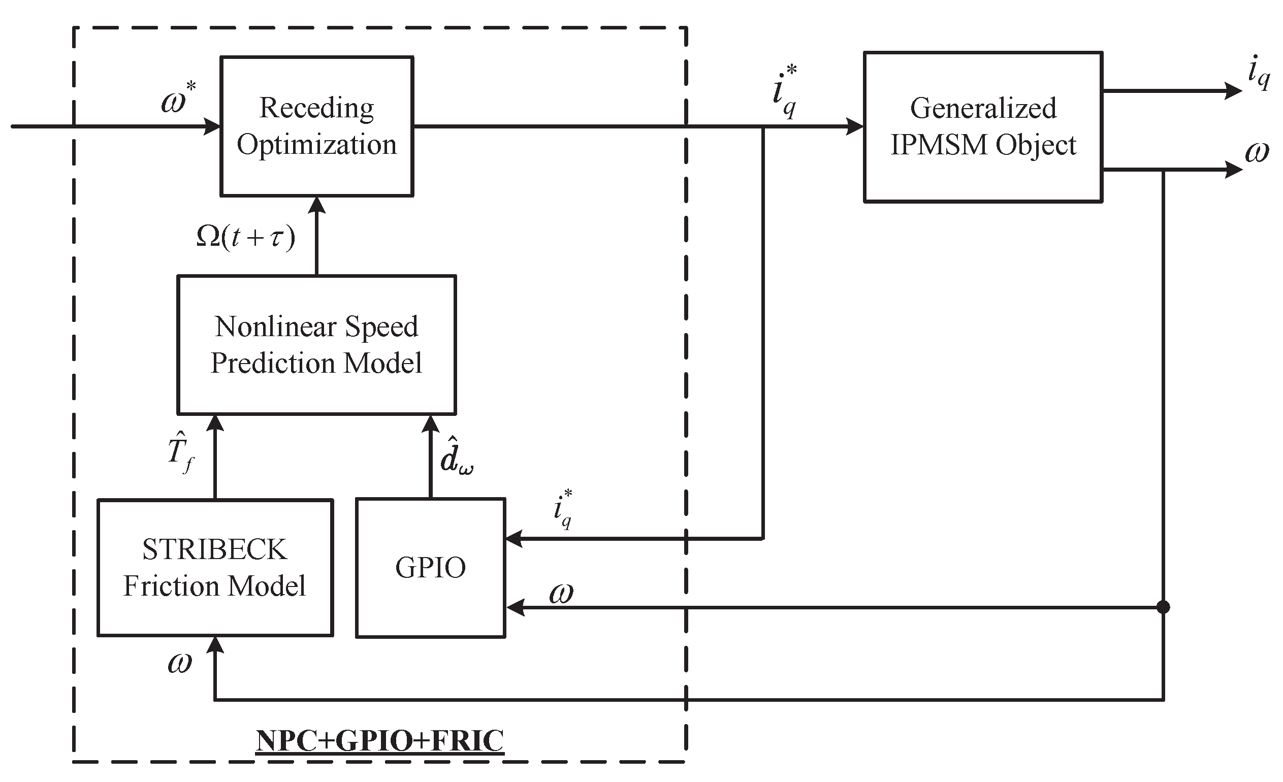
Remark 7. 

The speed control law given by Equation (36) is employed by the proposed nonlinear predictive control based on friction compensation and the GPI observer, and it can be abbreviated as NPC + GPIO + FRIC. For comparison, we also provide the control law using nonlinear predictive control based on the GPI observer without friction compensation (NPC + GPIO), given by

$$\begin{array}{c}\hfill u=-G^{-1}\left(x\right)\left(K_T{M}_{\rho }+L_f^{1}h\left(x\right)-{\dot{y}}_r\right)-g_2{g}_1^{-1}{v}_2.\end{array}$$

(37)

The entire control block diagram of the proposed nonlinear speed predictive control based on friction compensation and the GPI observer is shown in Figure 3, where ${\widehat{T}}_f$ represents represents the identified friction torque.

Remark 8 

(Robustness against the error of friction model). When the proposed symmetrical Stribeck friction model is extended to different mechanical mechanisms, friction test measurements are required in each case. It should be noted that even for the same type of mechanical mechanism, such as a ball screw, the friction model may exhibit subtle differences when the specification is varying. Occasionally, certain friction data measurement points inevitably contain some errors. Therefore, there is a strong need for a composed control method that exhibits high robustness against friction measurement errors. In this paper, the proposed method treats modeling errors as part of a lumped disturbance, which is estimated via GPIO, and a new predictive model is obtained for control, ensuring the robustness of the approach.

3.7. Convergence Analysis

Assumption 1. 

For the nonlinear time-varying model of speed dynamics (17), at least n time derivatives of the disturbance d exist.

Assumption 2. 

The disturbance $d\left(t\right)$ has a constant value in a steady state, i.e., $\underset{t\to \infty }{lim}\dot{d}=0$.

The closed-loop convergence of the velocity controller for the designed electromechanical servo system is guaranteed by the following theorem.

Theorem 1. 

Suppose that assumptions 1 and 2 are satisfied, and the disturbance observation error gain matrix is defined as

$$\begin{array}{c}\hfill A_{ev}=\left[\begin{array}{ccccc}-{\beta }^1& 1& 0& \dots & 0\\ -{\beta }^2& 0& 1& \dots & 0\\ \dots & & & & \\ -{\beta }^n& 0& 0& \dots & 1\\ -{\beta }^{n+1}& 0& 0& \dots & 0\end{array}\right],i=1,2,...,n+1.\end{array}$$

(38)

If the parameters ${\beta }^i,i=1,2,...,n+1$ are designed such that the disturbance observation error gain matrix $A_{ev}$ is Hurwitz stable, then the closed-loop system (17) will converge under the control input (36).

Proof. 

By substituting Equations (35)–(36) into Equation (27), $y\left(t\right)$ and $y^{\left[1\right]}\left(t\right)$ can be obtained as

$$\begin{array}{cc}\hfill y\left(t\right)& =L_f^{0}h\left(x\right)=\omega =x,\hfill \\ \hfill y^{\left[1\right]}\left(t\right)& =L_f^{1}h\left(x\right)+L_g^{1}h\left(x\right)\left[-G^{-1}\left(x\right)\left(K_T{M}_{\rho }+L_f^{1}h\left(x\right)-{\dot{y}}_r\right)+g_2{g}_1^{-1}{\widehat{T}}_f-g_2{g}_1^{-1}{v}_2\right]\hfill \\ \hfill & =f\left(x\right)+g_{2}d+K_T{M}_{\rho }-f\left(x\right)+{\dot{y}}_r-g_2\widehat{d}\hfill \\ \hfill & =K_T{M}_{\rho }+g_{2}d+{\dot{y}}_r-g_2\widehat{d}.\hfill \end{array}$$

(39)

Define the tracking error $e\left(t\right)$ as

$$\begin{array}{c}\hfill e\left(t\right)=y_r\left(t\right)-y\left(t\right),\end{array}$$

(40)

and substitute Equation (39) into Equation (40); the derivative of e can be given by

$$\begin{array}{c}\hfill \dot{e}={\dot{y}}_r-\dot{y}=-K_{T}e+g_{2}d-g_2\widehat{d}.\end{array}$$

(41)

Define the estimation error of the velocity dynamic GPI observer (22) as

$$\begin{array}{c}\hfill e_v=\left[\begin{array}{c}{e}_{v1}\\ e_{v2}\\ ⋮\\ e_{vn}\\ e_{vn+1}\end{array}\right]=\left[\begin{array}{c}x-v^1\\ d-v^2\\ ⋮\\ d^{\left(n-1\right)}-v^n\\ d^{\left(n\right)}-v^{n+1}\end{array}\right],\end{array}$$

(42)

and construct a new error vector $E\left(t\right)$ consisting of the tracking error $e\left(t\right)$ and the estimation error $e_v\left(t\right)$, given by

$$\begin{array}{c}\hfill E\left(t\right)={\left[\begin{array}{cc}e\left(t\right)& e_w\left(t\right)\end{array}\right]}^T.\end{array}$$

(43)

Let $\overline{d}\left(t\right)={\left[\begin{array}{cc}d\left(t\right)& \dot{d}\left(t\right)\end{array}\right]}^T,{\overline{g}}_2=\left[\begin{array}{ccccc}0& g_2& 0& \cdots & 0\end{array}\right],$ and the error dynamics equation of the entire closed-loop system is given by

$$\begin{array}{c}\hfill \dot{E}\left(t\right)=A_{\Sigma }E\left(t\right)+{\overline{G}}_{\Sigma }\overline{d}\left(t\right),\end{array}$$

(44)

where

$$\begin{array}{c}\hfill A_{\Sigma }=\left[\begin{array}{cc}-K_T& {\overline{g}}_2\\ 0& A_{ev}\end{array}\right],{\overline{G}}_{\Sigma }=\left[\begin{array}{cc}0& 0\\ 0& I\end{array}\right].\end{array}$$

(45)

Since $T_P>0$, $-K_T$ is Hurwitz stable. Therefore, as long as the parameters ${\alpha }^i,i=1,2,...,n+1$ are designed such that $A_e$ is Hurwitz stable, the close-loop system (17) under the control input (36) is convergent. □

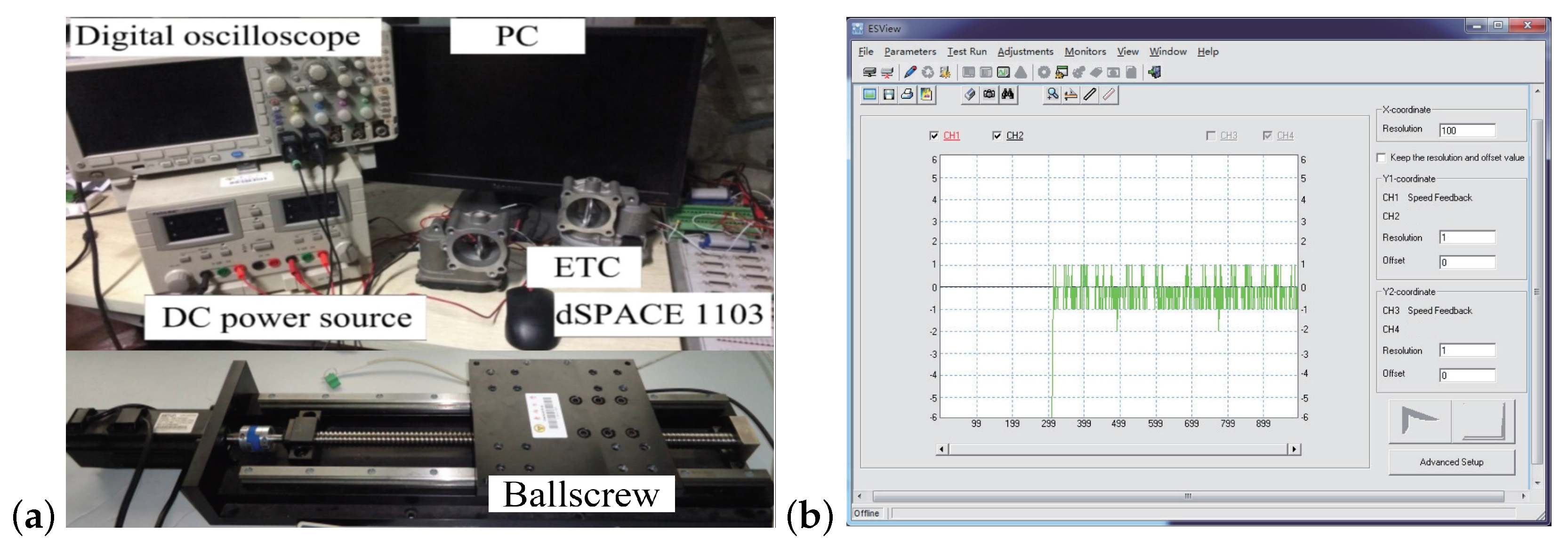
4. Experimental Validation

In this section, a series of experiments are detailed on a DSP-based IPMSM servo system. The experimental setup is shown in Figure 4. The processor used in the experimental drive is a fixed-point DSP (TMS3202812). The PWM period was set to 100 $\mathsf{\mu }$s, with a dead-time of 3.2 $\mathsf{\mu }$s. The power driving circuit consists of a single-phase diode bridge rectifier, a large capacitor filter, and an IGBT inverter. The DC link voltage is 310 V. The phase currents are measured using Hall-effect sensors, and the rotor position is detected by a 17-bit absolute encoder. The experimental motor is an eight-pole IPMSM, and its nominal parameters are provided in

Table 1. Motor nominal parameters.

Parameters	Value	Parameters	Value
Rated power P	750 (W)	Stator inductance on d-axis $L_d$	3.5 (mH)
Rated voltage $U_N$	200 (V)	Stator inductance on q-axis $L_q$	4 (mH)
Rated current $I_N$	4.5 (A)	Rotor inertia $J_N$	1.76$\times {10}^{-4}$ (kg $·{\mathrm{m}}^2)$
Rated torque $T_N$	2.4 (Nm)	Stator resistance $R_s$	1.74 ($\Omega$)
Rated speed $n_N$	3000 (rpm)	Flux linkage ${\psi }_f$	0.1267 (Wb)
Maximum speed $n_{max}$	6000 (rpm)	Torque constant $K_t$	0.5422 (Nm/A)
Pole pairs $n_P$	4	Viscous coefficient B	$7.388\times {10}^{-5}$ (Nm$·\mathrm{s}/\mathrm{rad})$

.

To illustrate the superiority of the proposed control method (NPC + GPIO + FRIC), experiments were carried out to compare NPC + GPIO, the integral control (NPC + I), and the traditional PI control. The effectiveness of these controllers was evaluated in both current control and speed control modes, addressing nonlinear cross-coupling effects and motor parameter variations to simulate diverse operating conditions and ensure an unbiased comparative analysis.

To demonstrate the advantages of the proposed control method (NPC + GPIO + FRIC), experiments were conducted to compare it with NPC + GPIO, the integral control (NPC + I), and the traditional PI control. The control performance of each controller was comprehensively compared and fairly evaluated under the same experimental conditions. The experiments were conducted on both a dynamometer loading system and a ball screw system.

Remark 9. 

Using an integrator to compensate for the disturbance d, the speed control law of NPC + I is given by

$$\begin{array}{c}\hfill u=-G^{-1}(x)(K_T{M}_{\rho }+L_f^{1}h\left(x\right)-{\dot{y}}_r)-g_2{g}_1^{-1}{y}_I,\end{array}$$

(46)

where

$$\begin{array}{c}\hfill y_I=K_I{\int }_0^t(\omega -{\omega }^{*})dt.\end{array}$$

(47)

The control parameters of the speed loop controller are shown in

Table 2. Experimental control parameter settings.

Controller	Parameters of the Controller
NPC + GPIO	Order of the GPI Observer = 4, ${\alpha }_1=16$, ${\alpha }_2=192$, ${\alpha }_3=1024$, ${\alpha }_4=2048$,
	$L_d$, $L_q$ and ${\psi }_f$ take 130% of the nominal value, B takes 60% of the nominal value, J takes the nominal value
NPC + I	$K_I=30$, $L_d$, $L_q$ and ${\psi }_f$ take 130% of the nominal value, B takes 60% of the nominal value
PI	$K_P=0.03$, $K_I=30$

, and a proportional control is uniformly used for the position loop, with the proportional gain set to 100.

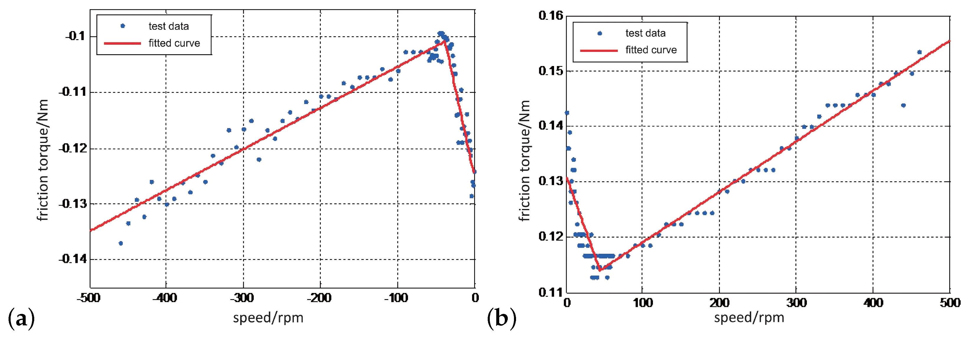
Based on the Stribeck friction characteristics, in the ultra-low-speed range of $-100⩽\omega ⩽100$ rpm, due to the strong nonlinearity of friction, the sampling interval is set to 1 rpm. For speed ranges where the absolute value of the rotational speed exceeds 100 rpm, the sampling interval is set to 10 rpm. The sampling results are shown as scatter points in Figure 5. The eight Stribeck linearized friction model identification results, obtained using the matrix-based least squares method, are shown in

Table 3. Stribeck segmented linearized friction model identification results.

Speed Range	Parameter Identification Results
$\omega ⩽-36$ rpm	${\alpha }_0=-0.1005$ N·m	${\alpha }_1=6.5\times {10}^{-5}$ N·m/rpm
$-36\mathrm{rpm}<\omega <0$	${\beta }_0=-0.1252$ N·m	${\beta }_1=-6.3158\times {10}^{-4}$ N·m/rpm
$0⩽\omega <36$ rpm	${\gamma }_0=-0.2531$ N·m	${\gamma }_1=-5.1258\times {10}^{-4}$ N·m/rpm
$\omega ⩾36$ rpm	${\lambda }_0=0.1164$ N·m	${\lambda }_1=6.8\times {10}^{-5}$ N·m/rpm

, and the resulting fitting curve is shown in Figure 5.

4.1. Dynamometer Loading Experiment

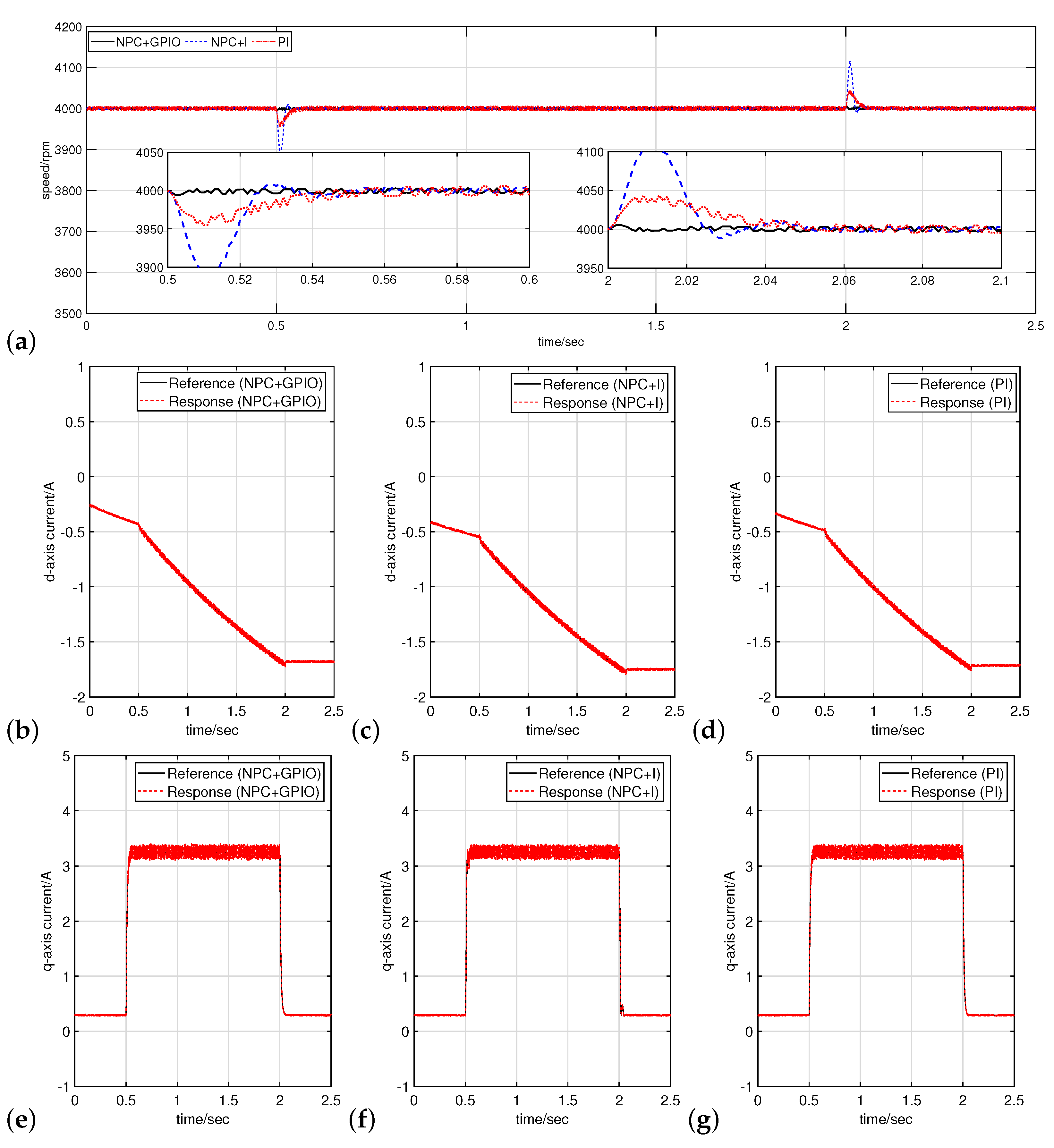
In this subsection, we detail the performed load surge and load removal tests using a dynamometer. Note that the dynamometer test platform does not exhibit nonlinear friction torque, so the control law of NPC + GPIO + FRIC is the same as that of NPC + GPIO. When the motor operates in a stable speed state, the dynamometer is used to apply sudden torque increases and decreases to test the load speed control performance under three controllers (NPC + GPIO, NPC + I, and PI).

Figure 6 and Figure 7, respectively, show the speed response waveforms for a given speed of 500 rpm with a sudden increase in and the removal of the rated torque of 2.4 N·m and for a given speed of 4000 rpm with a sudden increase in and the removal of the rated torque of 1.5 N·m. It is important to note that when the given speed is 4000 rpm, the motor operates in the constant power weak magnetic region, so the rated torque decreases compared to the region of constant torque. When the given speed is 500 rpm with a rated torque of 2.4 N·m, from Figure 6a and Figure 7a, it can be seen that the NPC + GPIO corresponding waveform shows the smallest decrease (or increase) in speed during load surge (or removal) and the shortest recovery time. This indicates that NPC + GPIO handles external disturbances caused by the load torque ($T_L$) in the electromechanical servo system more effectively. Specific speed control performance indicators against load are shown in

Table 4. Comparison of speed load resistance control performance indicators for three speed controllers (NPC + GPIO, NPC + I, and PI) (dynamometer loading experiment).

Experimental Conditions	Speed Controller	Current Controllers	Load Torque	Sudden Increase		Sudden Decrease
				Decay (rpm)	Recovery Time (ms)	Rise (rpm)	Recovery Time (ms)
500 rpm dynamometer	NPC + GPIO	NPC + GPIO	2.4 Nm	12	6.8	14	7.2
	NPC + I			28	12.3	31	13.4
	PI			79	78.2	77	79.6
4000 rpm dynamometer	NPC + GPIO	NPC + GPIO	1.5 Nm	14	5.8	15	6.1
	NPC + I			48	21.2	51	20.8
	PI			116	68.5	125	69.2

. Since the current loop uses the NPC + GPIO inner controller, it is worth mentioning that there were no steady-state fluctuations during weak magnetic loading, as observed in the experiments of the previous chapter.

4.2. Ball Screw Experiment

In the ball screw experiment, the control performance of three speed controllers (NPC + GPIO, NPC + I, and PI) under the position of closed-loop control mode with a flexible load was first tested. The position loop uses P control with a proportional gain of 100, and the reference position is a sinusoidal signal ${\theta }^{*}=sin\left(0.667\times 2\pi t\right)rad$ with an amplitude of 1 rad and a frequency of 0.667 Hz. 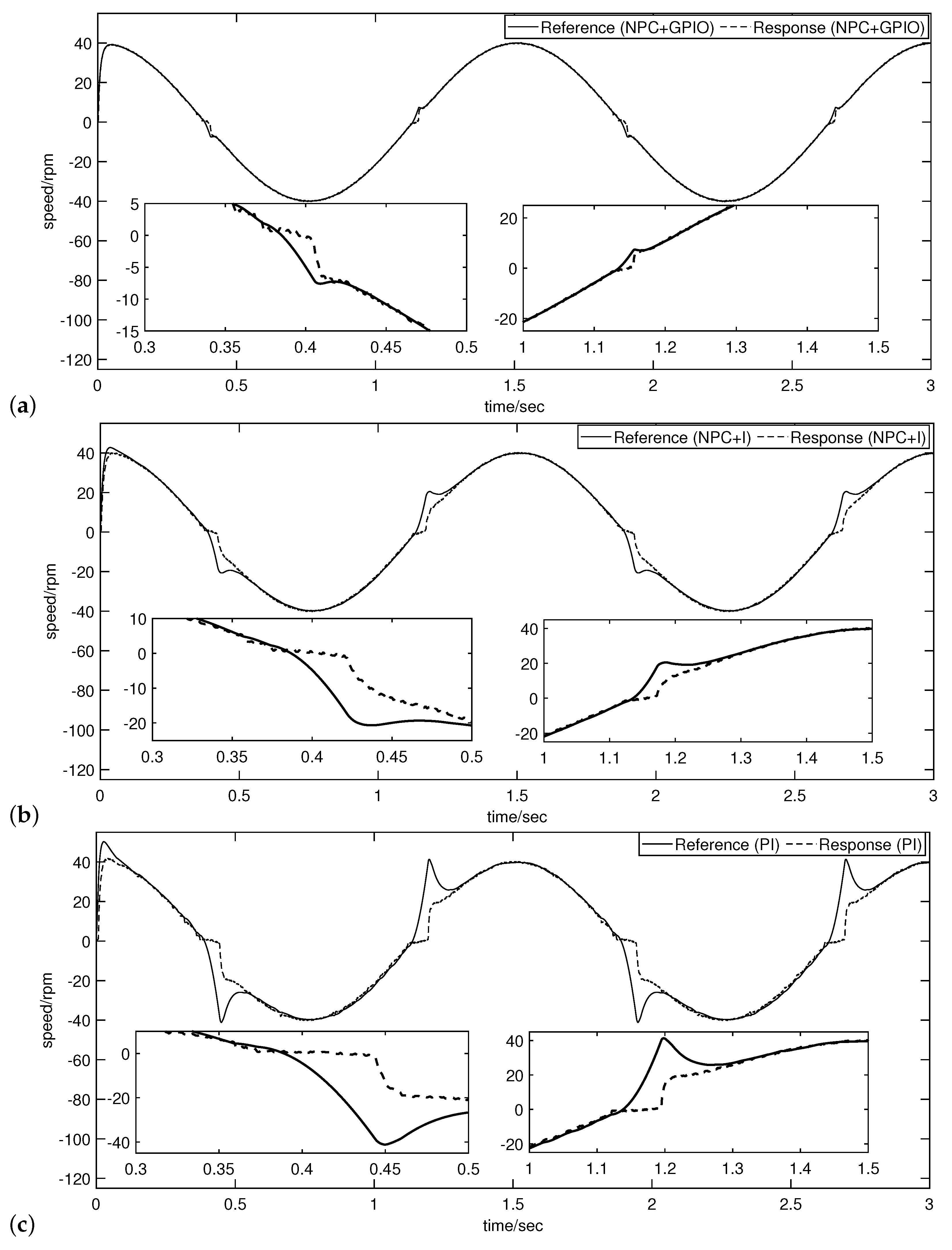Figure 8 shows the position response waveforms under the influence of the three speed controllers. It can be observed that the position response waveforms for all three controllers exhibit position tracking distortion at both the peaks and valleys, which is known as the “flat-top” phenomenon in the industry. The distortion is most severe for the velocity loop PI controller, followed by NPC + I, and NPC + GPIO performs slightly better, although the distortion is still quite evident. Figure 9 shows the speed response waveforms under the influence of the three speed controllers. It can be seen that all three controllers exhibit speed tracking distortion near zero speed, and the time interval coincides with the “flat-top” phenomenon in position tracking. This is referred to as the “ramp-up” phenomenon near zero speed in the industry. The speed tracking distortion is most severe for the velocity loop PI controller, followed by NPC + I, and NPC + GPIO performs slightly better, though the distortion is still quite noticeable.

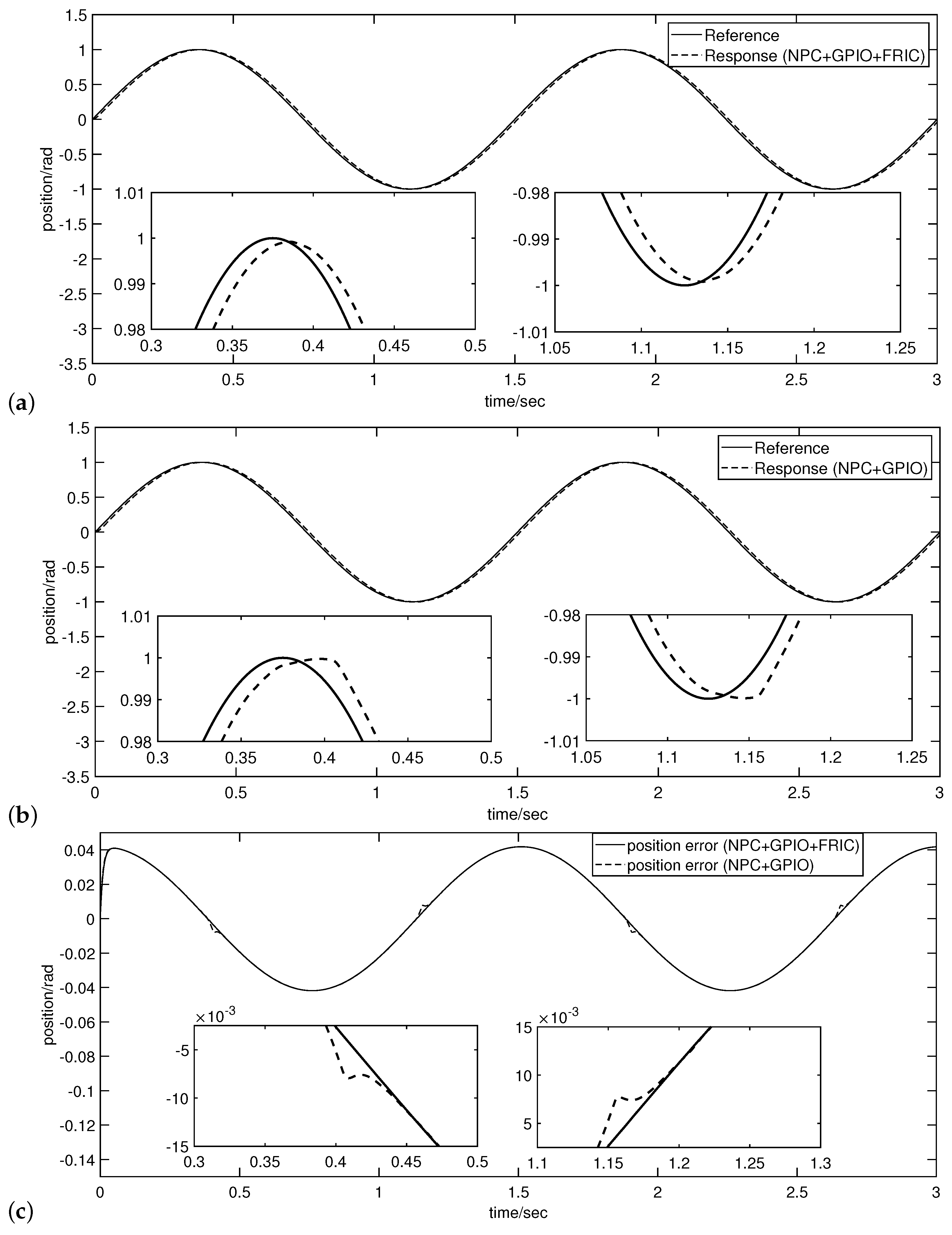
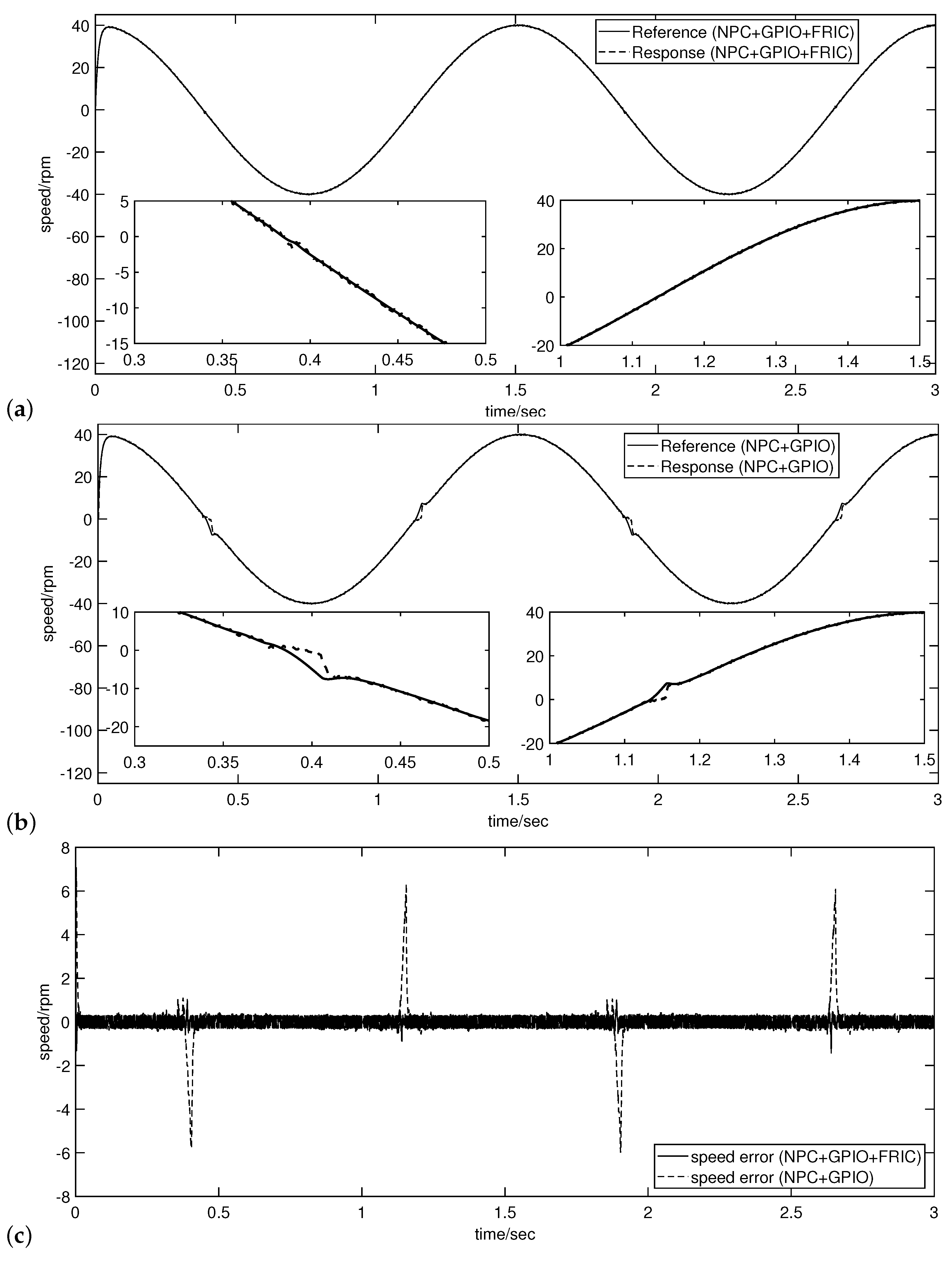
Next, a targeted comparison is made between NPC + GPIO + FRIC and NPC + GPIO. The given position is a sinusoidal signal with an amplitude of 1 rad and a frequency of 0.667 Hz: (${\theta }^{*}=sin\left(0.667\times 2\pi t\right)rad$). Figure 10 shows the position response waveforms under the influence of two speed controllers (NPC + GPIO + FRIC and NPC + GPIO). It can be seen that, compared to NPC + GPIO, the position response waveform of NPC + GPIO + FRIC does not exhibit position distortion at the peaks and valleys, resolving the “flat-top” phenomenon in the commutation region. 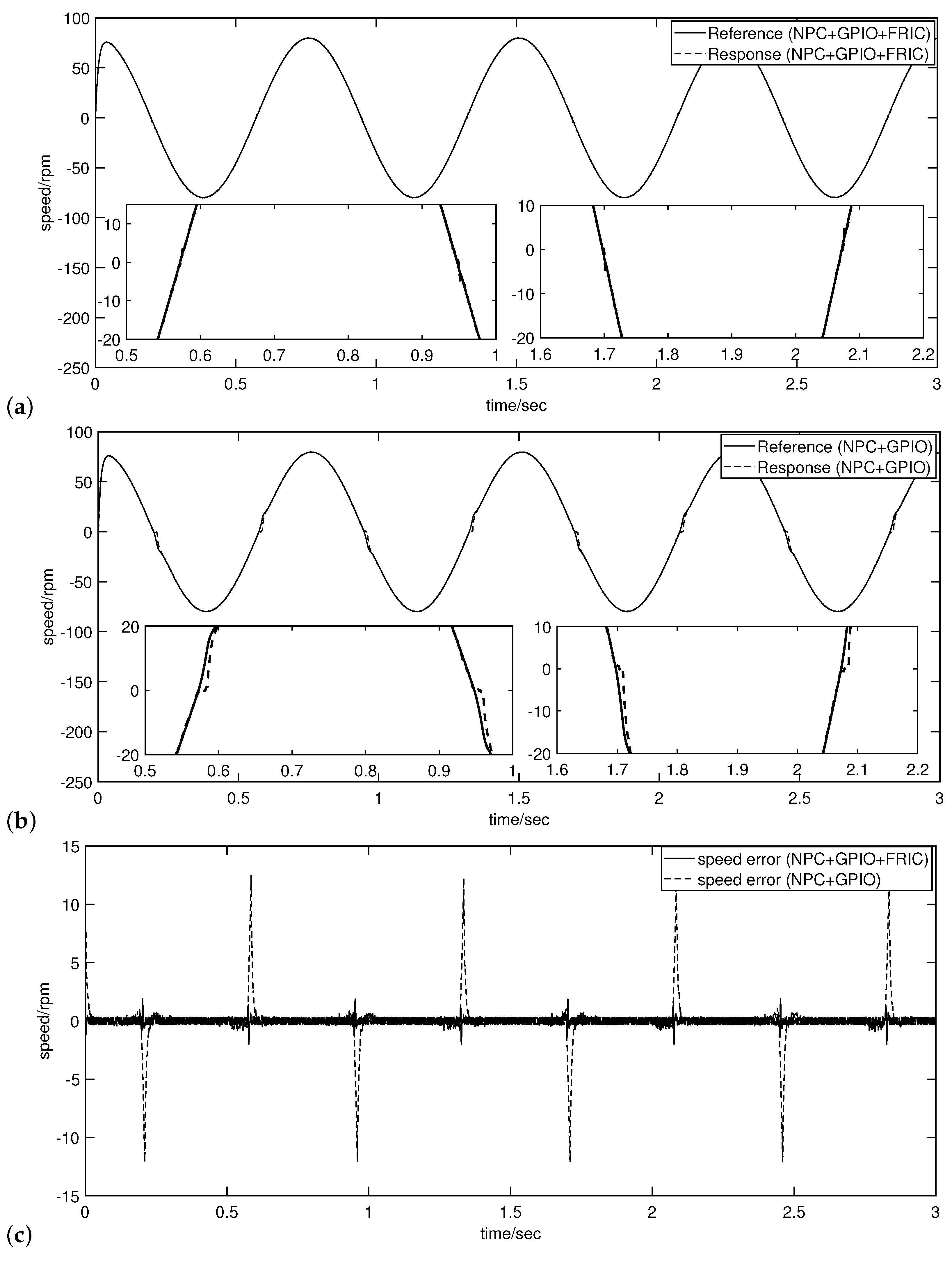Figure 11 shows the speed response waveforms under the influence of the two speed controllers. It can be observed that NPC + GPIO + FRIC exhibits minimal distortion in the speed range near zero, resolving the “ramp-up” phenomenon near zero speed.

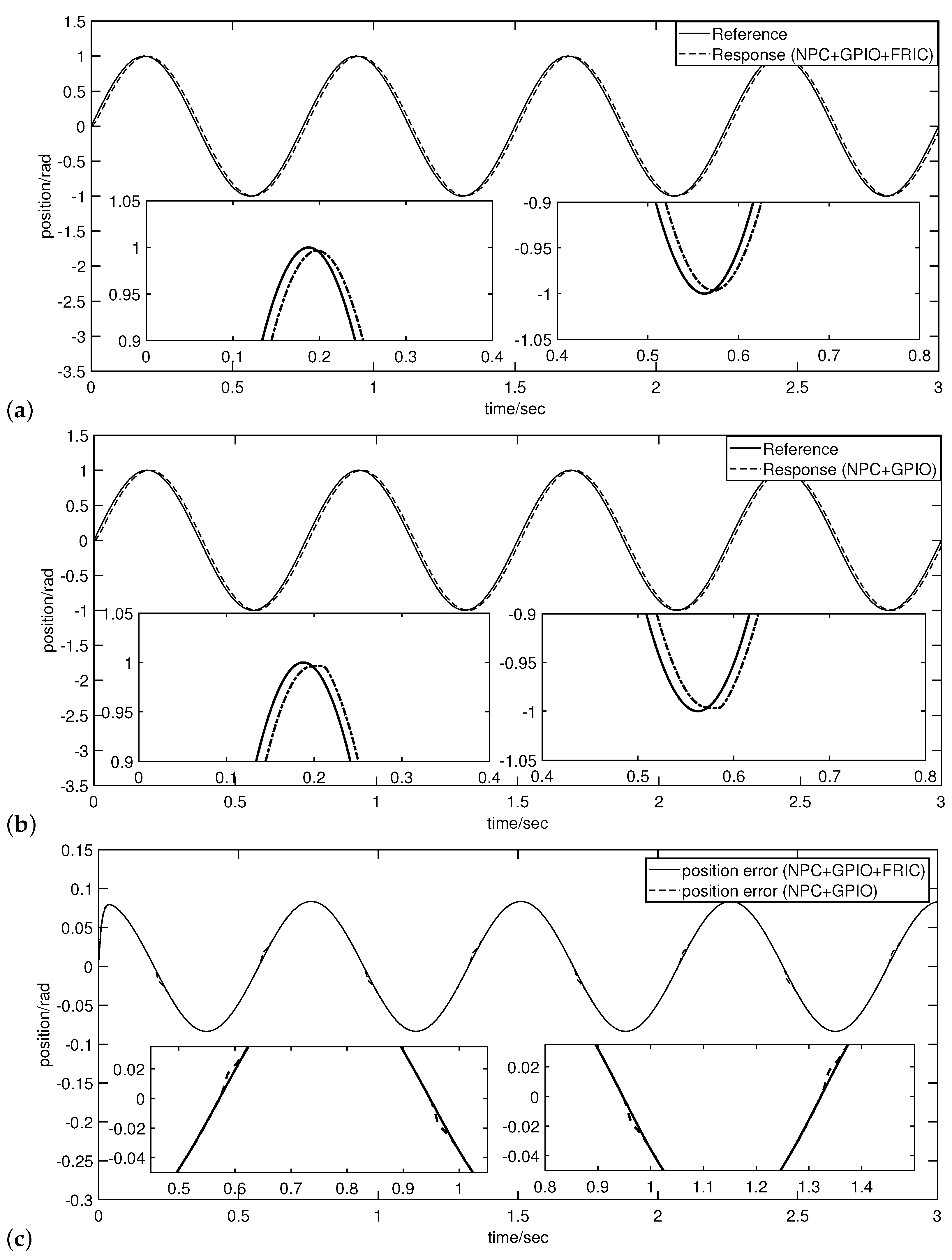
When the frequency of the position sinusoidal signal is doubled, i.e., the given position is a sinusoidal signal with an amplitude of 1 rad and a frequency of 1.333 Hz (${\theta }^{*}=sin\left(1.333\times 2\pi t\right)rad$), Figure 12 and Figure 13 still show that, compared to NPC + GPIO, the friction-compensated NPC + GPIO + FRIC controller solves the “flat-top” phenomenon in the commutation region and the “ramp-up” phenomenon near zero speed.

Overall, when examining Figure 10, Figure 11, Figure 12 and Figure 13, it can be observed that in the reciprocating motion test of the ball screw, the control effects of the PI, NPC + I, NPC + GPIO, and NPC + GPIO + FRIC methods mainly differ in their performance during critical velocity reversal regions, which aligns with the practical needs of the industry. Among these methods, the NPC + GPIO + FRIC approach proposed in this paper demonstrates the best suppression effect on both the “flat-top” and the “ramp-up” phenomena during the reversal regions, making it a promising solution to address relevant industrial needs.

5. Conclusions

In this study, to improve the speed control performance of an IPMSM electromechanical servo system under complex conditions of nonlinear friction torque and time-varying parameters, a nonlinear speed predictive control method (NPC + GPIO + FRIC) was designed based on symmetry-inspired Stribeck segmented linear friction compensation and a GPI observer. Comparisons between the integral NPC scheme and the conventional PI control scheme have demonstrated its superiority. Load experiments using a dynamometer and ball screw experiments were conducted on a DSP-based IPMSM electromechanical servo system. The experimental results validate that the proposed method effectively eliminates the position “flat-top” and speed “ramp-up” phenomena caused by nonlinear friction, and a satisfactory speed control performance has been achieved. Furthermore, in response to potential widespread industrial-scale adoption and application, engineers can incorporate automated parameter identification for the friction model proposed in this paper into servo products, thereby replacing the manual modeling and testing process.

References

1. Gan, H.; Cao, Z.; Chen, P.; Luo, Y.; Luo, X. Fractional-order electromagnetic modeling and identification for PMSM servo system. ISA Trans. 2024, 147, 527–539. [Google Scholar] [CrossRef] [PubMed]
2. Zhang, K.; Ma, J.; Lu, J.; Liu, Y.; Qiu, L.; Liu, X.; Fang, Y. Nonlinear flux observer for sensorless control of IPMSM based on a novel regression model. IEEE Trans. Power Electron. 2025, 40, 3916–3926. [Google Scholar] [CrossRef]
3. Tang, M.; Zhuang, S. On speed control of a permanent magnet synchronous motor with current predictive compensation. Energies 2019, 12, 65. [Google Scholar] [CrossRef]
4. Yang, Z.; Qian, C.; Sun, X.; Wang, K. Enhanced linear ADRC strategy for sensorless control of IPMSM considering cross-coupling factors. IEEE Trans. Transp. Electrif. 2023, 9, 4437–4446. [Google Scholar] [CrossRef]
5. Gou, M.; Wang, B.; Zhang, X. Development of multi-motor servo control system based on heterogeneous embedded platforms. Electronics 2024, 13, 2957. [Google Scholar] [CrossRef]
6. Song, Z.; Zhou, W.; Mo, Y. Research on predictive speed control scheme for surface-mounted permanent magnet servo systems. Electronics 2024, 13, 3421. [Google Scholar] [CrossRef]
7. Chen, S.; Ding, W.; Wu, X.; Huo, L.; Hu, R.; Shi, S. Sensorless control of IPMSM drives using high-frequency pulse voltage injection with random pulse sequence for audible noise reduction. IEEE Trans. Power Electron. 2023, 38, 9395–9408. [Google Scholar] [CrossRef]
8. Quintal-Palomo, R.E. Analysis of current signals in a partially demagnetized vector controlled interior permanent magnet generator. Power Electron. Drives 2019, 4, 179–190. [Google Scholar] [CrossRef]
9. Cui, Y.; Yin, Z.; Gao, F.; Zhang, Y.; Liu, Y.; Liu, J. Speed control of IPMSM based on series connection leading correction linear active disturbance rejection. IEEE Trans. Power Electron. 2024, 39, 3096–3108. [Google Scholar] [CrossRef]
10. Zuo, Y.; Wang, H.; Ge, X.; Zuo, Y.; Woldegiorgis, A.T.; Feng, X.; Lee, C.H. A novel current measurement offset error compensation method based on the adaptive extended state observer for IPMSM drives. IEEE Trans. Ind. Electron. 2024, 71, 3371–3382. [Google Scholar] [CrossRef]
11. Mohammed, S.A.Q.; Al-kaf, H.A.G.; Lee, K.B. Robust hybrid current control approach for IPMSM drives subjected to system uncertainty. IEEE Transactions on Industrial Electronics. IEEE Trans. Ind. Electron. 2024, 71, 15532–15542. [Google Scholar] [CrossRef]
12. Yuan, S.; Deng, W.; Liang, X.; Yao, J.; Yang, G. Nonlinear robust adaptive precision motion control of motor servo systems with unknown actuator backlash compensation. ISA Trans. 2023, 137, 349–357. [Google Scholar] [CrossRef]
13. Ohishi, K.; Haga, H.; Abe, K. Survey and analysis for high power factor IPMSM drive system using electrolytic capacitor-less inverter. IEEJ Trans. Electr. Electron. Eng. 2024, 19, 1432–1445. [Google Scholar] [CrossRef]
14. Lin, Q.; Liu, L.; Liang, D. Joint Estimation of Resistance and Speed With Auxiliary State of Active Flux for Sensorless IPMSM Drives. IEEE Trans. Ind. Electron. 2023, 71, 10356–10365. [Google Scholar] [CrossRef]
15. Park, H.J.; Ahn, H.W.; Go, S.C. A study on performance and characteristic analysis according to the operating point of IPMSM drive. Energies 2023, 16, 1219. [Google Scholar] [CrossRef]
16. Li, W.; Fan, X.; Zhu, L.; Chen, W. A dynamic hysteresis-based iron loss calculation method and its application in a PWM-Fed IPMSM. IEEE Trans. Energy Convers. 2024, 39, 1738–1749. [Google Scholar] [CrossRef]
17. Wang, C.; Peng, J.; Pan, J. A novel friction compensation method based on Stribeck model with fuzzy filter for PMSM servo systems. IEEE Trans. Ind. Electron. 2023, 70, 12124–12133. [Google Scholar] [CrossRef]
18. Rsetam, K.; Cao, Z.; Man, Z. Cascaded-extended-state-observer-based sliding-mode control for underactuated flexible joint robot. IEEE Trans. Ind. Electron. 2019, 67, 10822–10832. [Google Scholar] [CrossRef]
19. Jing, C.; Zhang, H.; Yan, B.; Hui, Y.; Xu, H. State and disturbance observer based robust disturbance rejection control for friction electro-hydraulic load simulator. Nonlinear Dyn. 2024, 112, 17241–17255. [Google Scholar] [CrossRef]
20. Yao, X.; Zhang, L.; Cui, Y. Adaptive refined disturbance observer-based velocity-tracking control for gimbal servo system with multiple disturbances. IEEE Trans. Syst. Man Cybern. Syst. 2024, 54, 7170–7181. [Google Scholar] [CrossRef]
21. Klarecki, K.; Rabsztyn, D. Hydraulic measuring hoses as pressure signal distortion—mathematical model and results of experimental tests. Sensors 2023, 23, 7056. [Google Scholar] [CrossRef] [PubMed]
22. Zhao, J.; Du, J.; Zhu, B.; Chen, Z. Adaptive dual-loop pressure control for an integrated electro-hydraulic brake system considering uncertain nonlinear characteristics. IEEE Trans. Transp. Electrif. 2024, 10, 9428–9440. [Google Scholar] [CrossRef]
23. Sun, Z.; Qiu, J.; Zhu, J.; Li, S. A composite position control of flexible lower limb exoskeleton based on second-order sliding mode. Nonlinear Dyn. 2023, 111, 1657–1666. [Google Scholar] [CrossRef]
24. Saha, B.; Singh, B. Torque ripple mitigation in sensorless PMBLDC motor drive with adaptive observer for LEV. IEEE Trans. Power Electron. 2024, 40, 1739–1747. [Google Scholar] [CrossRef]
25. Jeong, Y.W.; Chung, C.C. Observer-based robust control: Its application to permanent magnet synchronous motors. IEEJ J. Ind. Appl. 2023, 12, 575–587. [Google Scholar] [CrossRef]
26. Chen, P.; Luo, Y.; Gan, H.; Liu, Y.; Chen, Y. A current and speed loop decoupling controller for SPMSM under periodic disturbances. IEEE Trans. Power Electron. 2024, 39, 6889–6902. [Google Scholar] [CrossRef]
27. Zhang, P.; Shi, Z.; Yu, B. Research on friction compensation method of electromechanical actuator based on improved active disturbance rejection control. Actuators 2023, 12, 445. [Google Scholar] [CrossRef]
28. Wang, B.; Jin, H.; Yin, H.; Liu, Z.; Zhao, J. Friction dynamics identification based on quadratic approximation of LuGre model. Nonlinear Dyn. 2024, 112, 6357–6377. [Google Scholar] [CrossRef]
29. Hu, S.; Wan, Y.; Liang, X. Adaptive fast terminal sliding mode control of robotic manipulators based on joint torque estimation and friction compensation. Int. J. Robust Nonlinear Control. 2024, 34, 12223–12238. [Google Scholar] [CrossRef]
30. Zhou, K.; Ai, M.; Sun, D.; Jin, N.; Wu, X. Flatness and defect of non-linear systems: Introductory theory and examples. Energies 2012, 12, 4526. [Google Scholar] [CrossRef]
31. Chen, W.-H.; Yang, J.; Guo, L.; Li, S. Disturbance-observer-based control and related methods-An overview. IEEE Trans. Ind. Electron. 2015, 63, 1083–1095. [Google Scholar] [CrossRef]
32. Wu, C.; Yang, J.; Li, S.; Li, Q.; Guo, L. Disturbance observer based model predictive control for accurate atmospheric entry of spacecraft. Adv. Space Res. 2018, 61, 2457–2471. [Google Scholar] [CrossRef]
33. Wu, C.; Yang, J.; Li, Q. GPIO-based nonlinear predictive control for flux-Weakening current control of the IPMSM servo system. Energies 2020, 13, 1716. [Google Scholar] [CrossRef]
34. Loganathan, M.K.; Gandhi, O.P. Reliability enhancement of manufacturing systems through functions. Proc. Inst. Mech. Eng. Part B J. Eng. Manuf. 2015, 231, 1850–1868. [Google Scholar] [CrossRef]
35. Loganathan, M.K.; Gandhi, M.S.; Gandhi, O.P. Functional cause analysis of complex manufacturing systems using structure. Proc. Inst. Mech. Eng. Part B J. Eng. Manuf. 2014, 229, 533–545. [Google Scholar] [CrossRef]
Figure 1. Block diagram of the speed control for the generalized IPMSM object.
Symmetry 17 01012 g001
Figure 2. Stribeck friction characteristic curve and segmentation diagram.
Symmetry 17 01012 g002
Figure 3. Block diagram of the proposed speed control method for the generalized IPMSM object.
Symmetry 17 01012 g003
Figure 4. The experiment platform: (a) the tested IPMSM servo system; (b) the software interface of the upper computer.
Symmetry 17 01012 g004
Figure 5. Stribeck friction model identification results: (a) Reverse rotation; (b) forward rotation.
Symmetry 17 01012 g005
Figure 6. Comparison of waveforms for three speed controllers (NPC + GPIO, NPC + I, and PI) at a given speed of 500 rpm (with the low- and medium-speed range degraded to i d = 0 control) (dynamometer loading: 2.4 N·m): (a) Comparison of speed response waveforms for the three speed controllers; (b) d-axis current response waveform under NPC + GPIO speed controller; (c) d-axis current response waveform under NPC + I speed controller; (d) d-axis current response waveform under PI speed controller; (e) q-axis current response waveform under NPC + GPIO speed controller; (f) q-axis current response waveform under NPC + I speed controller; (g) q-axis current response waveform under PI speed controller.
Symmetry 17 01012 g006
Figure 7. Comparison of waveforms for three speed controllers (NPC + GPIO, NPC + I, and PI) at a given speed of 4000 rpm (high-speed range with field-weakening control) (dynamometer loading: 1.5 N·m): (a) Comparison of speed response waveforms for the three speed controllers; (b) d-axis current response waveform under NPC + GPIO speed controller; (c) d-axis current response waveform under NPC + I speed controller; (d) d-axis current response waveform under PI speed controller; (e) q-axis current response waveform under NPC + GPIO speed controller; (f) q-axis current response waveform under NPC + I speed controller; (g) q-axis current response waveform under PI speed controller.
Symmetry 17 01012 g007
Figure 8. Comparison of position response waveforms under the given position sinusoidal command (1 rad; 0.667 Hz) for three speed controllers (NPC + GPIO, NPC + I, and PI): (a) NPC + GPIO; (b) NPC + I; (c) PI.
Symmetry 17 01012 g008
Figure 9. Comparison of speed response waveforms under the given position sinusoidal command (1 rad; 0.667 Hz) for three speed controllers (NPC + GPIO, NPC + I, and PI): (a) NPC + GPIO; (b) NPC + I; (c) PI.
Symmetry 17 01012 g009
Figure 10. Comparison of position response waveforms under parameter-varying conditions with the given position sinusoidal command (1 rad; 0.667 Hz) for two speed controllers (NPC + GPIO + FRIC and NPC + GPIO): (a) NPC + GPIO + FRIC; (b) NPC + GPIO; (c) position tracking error for both controllers.
Symmetry 17 01012 g010
Figure 11. Comparison of speed response waveforms under parameter-varying conditions with the given position sinusoidal command (1 rad; 0.667 Hz) for two speed controllers (NPC + GPIO + FRIC and NPC + GPIO): (a) NPC + GPIO + FRIC; (b) NPC + GPIO; (c) Speed tracking error for both controllers.
Symmetry 17 01012 g011
Figure 12. Comparison of position response waveforms under parameter-varying conditions with the given position sinusoidal command (1 rad; 1.333 Hz) for two speed controllers (NPC + GPIO + FRIC and NPC + GPIO): (a) NPC + GPIO + FRIC; (b) NPC + GPIO; (c) position tracking error for both controllers.
Symmetry 17 01012 g012
Figure 13. Comparison of speed response waveforms under parameter-varying conditions with the given position sinusoidal command (1 rad; 1.333 Hz) for two speed controllers (NPC + GPIO + FRIC and NPC + GPIO): (a) NPC + GPIO + FRIC; (b) NPC + GPIO; (c) Speed tracking error for both controllers.
Symmetry 17 01012 g013