Abstract
In this study, we begin by extending the mathematical formulation of the expectile risk measure through a key modification: replacing the expectation in its defining equation with expected shortfall. This substitution leads to a revised risk measure that more precisely captures downside risk. To handle the uncertainty of the underlying distribution, we then adopt a distributionally robust optimization framework. Notably, this robust optimization problem can be reformulated as a linear programming problem, and by employing suitable approximation techniques, we derive an analytical solution. In numerical experiments, our portfolio problem exhibits superior performance when compared to several traditional and distributionally robust optimized portfolio problems.
MSC:
91G70
1. Introduction
In the context of portfolio optimization, while Markowitz’s [1] mean–variance question provides a theoretical foundation for asset allocation, its limitations have become increasingly evident in practical applications. Variance, as a risk measure, fails to distinguish between different types of risks and overlooks the distribution of risk, which may expose investors to unacceptable levels of loss. Additionally, parameter estimation errors, particularly in the covariance matrix and mean vector, can lead to significant variations in the optimization outcomes, thereby impacting the robustness of the portfolio [2].
To overcome these limitations, new risk measures have been proposed, with the expectile emerging as a prominent tool in both statistics and finance in recent years [3]. Compared to traditional risk measures such as the Value at Risk (VaR) and expected shortfall (ES), the expectile provides a more flexible approach to capturing different degrees of risk aversion by minimizing the weighted mean squared error. By adjusting parameter , the expectile allows for greater emphasis on either the lower or upper tail of the distribution, making it suitable for a variety of investment objectives. This method not only effectively complements traditional risk measures but also offers a more refined and personalized risk control strategy for portfolio optimization.
Formally, the -expectile [3] is defined by
where is the confidence level, denotes the positive part, and denotes the negative part. According to [4], is the unique solution to this optimization problem if and only if
When , the expectile coincides with the mean of X. As moves above , progressively exceeds the mean, reflecting an increasing focus on higher losses (or lower returns). Conversely, when , the expectile shifts below the mean, emphasizing outcomes below the central tendency. These features allow practitioners to adjust according to the severity of risks they wish to emphasize, providing a flexible measure that can better capture tail risks and adapt to changing market conditions. This makes the expectile a valuable tool for tailoring risk management strategies in investment portfolios.
In the application domain, ref. [3] demonstrates that expectiles serve as rigorous and efficient risk assessment tools, characterized by properties such as coherence, elicitability, non-negative risk margins, and adaptability to structured contracts. Building on this foundation, ref. [5] provides closed-form expectile(ERM) formulas via generalized Fourier inversion, validates them across five market models, and proposes a 1.25 ERM-to-VaR scaling for Basel compliance. As coherent measures (with ), expectiles enhance regulatory compliance and facilitate comprehensive risk verification, while optimal reinsurance strategies effectively streamline the trade-off between risk and cost.
Additionally, Taylor’s Conditional Autoregressive Expectiles (CARE) model [6] employs asymmetric least squares to capture autoregressive structures, enabling the dynamic estimation of VaR and ES without imposing restrictive distributional assumptions. Empirical evidence indicates that the CARE model attains accuracy comparable to that of historical simulation and GARCH-EVT approaches—especially in estimating extreme quantiles—thereby overcoming the limitation of Conditional Autoregressive Value-at-Risk methods, which focus solely on VaR, and ultimately offering a more comprehensive framework for financial risk management.
To further enhance the applicability of these tools, this paper introduces a generalization of the expectile concept to encompass expected shortfall at a confidence level , which assesses the anticipated value of losses across varying confidence levels. Moreover, this paper also attempts to use expectile for portfolio decision making. This generalization not only preserves the advantageous properties of expected shortfall but also integrates the flexibility inherent in the expectile, thereby facilitating a more comprehensive risk assessment that accommodates diverse risk preferences and confidence levels.
In this paper, we generalize the expectile, and its generalized form can be expressed as
In this equation, represents the expected shortfall at confidence level for the positive part of the loss , while corresponds to the expected shortfall for the negative part. The solution d to this equation is referred to as the ES-expectile, denoted as . When , .
The expected shortfall (ES) [7] is defined as
where the Value at Risk (VaR) at confidence level is mathematically defined as
Additionally, for ES, there is the Rockafellar–Uryasev formula [7], which simplifies the computation of the conditional risk measure ES. The value of is obtained by solving the following optimization problem:
This formulation emphasizes the use of different weights for losses above and below a specified threshold, under varying confidence levels, thereby capturing the severity of extreme risk scenarios more effectively than traditional measures such as VaR.
To address this uncertainty, distributionally robust optimization (DRO) has been proposed as an effective modeling technique. The main objective of DRO is to find decisions that minimize the worst-case expected cost over an ambiguity set, which is constructed using the distributional information of uncertain data. Compared to traditional robust optimization, DRO utilizes available distributional information more effectively, making it a more conservative approach in handling uncertainty [8].
In recent years, distributionally robust optimization methods based on Wasserstein ambiguity sets have gained significant attention. To the best of our knowledge, Mohajerin Esfahani and Kuhn [9] first explored the convex reformulation of the Wasserstein distributionally robust optimization question, demonstrating several desirable properties of this approach. Gao subsequently extended these properties and explored the connection between distributionally robust optimization and variation regularization [10,11]. Today, DRO is widely applied in various fields, including machine learning [12] and portfolio optimization [13,14,15,16,17,18].
We summarize our main contributions in this paper as follows:
- Expected Shortfall Expectile (ES-expectile). We introduce a new class of risk measures by substituting the expectation in the classical expectile definition with expected shortfall (ES). This modification preserves the coherent risk measure spirit of ES while maintaining the sensitivity of expectiles to the full distribution, yielding a refined metric that captures the entire left-tail risk profile more faithfully than either the ES or expectile alone.
- Distributionally Robust ES-expectile via Wasserstein Ambiguity. To counter the instability arising from finite-sample empirical distributions, we formulate the ES-expectile portfolio problem within a distributionally robust optimization framework whose ambiguity set is a Wasserstein ball centered at the empirical distribution. We prove that the resulting min–max problem can be conservatively reformulated as a computationally tractable program that can be solved reliably with standard optimization software.
- Empirical Superiority and Extreme-Weight Adjustment. Out-of-sample experiments show that our distributionally robust ES-expectile question (DRES-expectile) delivers higher Sharpe ratios and Sortino ratios compared with the classical ES-expectile portfolio question, traditional portfolio approaches, and Wasserstein DRO portfolios. Although the DRES-expectile occasionally yields extreme allocations, we mitigate this behaviour with a lightweight extreme-weight adjustment heuristic that retains most of the performance gains while reducing variance.
The remainder of this paper is organized as follows. In Section 2, the definition of the ES-expectile is presented, and its favorable properties are demonstrated through a series of lemmas and theorems, culminating in the introduction of the ES-expectile question. Section 3 begins with an introduction to the theory of distributionally robust optimization along with related theorems. Based on this foundation, the DRES-expectile is derived, and its degenerate form is also presented. Section 4 further simplifies the DRES-expectile question, and Section 5 presents numerical experiments that highlight the unique features of our question and provide guidance for portfolio adjustment decisions. The results indicate that our question outperforms both traditional portfolio questions and those based on distributionally robust optimization. Section 6 provides a dedicated discussion of the managerial and investor implications of the proposed DRES-expectile framework and translates the empirical evidence into actionable guidance for future portfolio optimization practice.
For clarity and ease of reference, Table 1 lists the key symbols and abbreviations employed in this paper.

Table 1.
Comprehensive list of symbols and acronyms.
Notations: We denote by the Dirac measure concentrated at , which assigns a unit mass to point . The empirical distribution is then defined as the probability measure given by the average where are the observed samples. We denote by the vector where each component is 1. We denote by the indicator function, which assigns a value of 1 if , and 0 otherwise. We denote by the set of all Borel probability measures supported on , where . Let represent an atomless probability space, where is the set of possible states, is a -algebra on , and is the probability measure. The space refers to the set of measurable functions f for which .
2. ES-Expectile
In this section, we will define the ES-expectile question and derive some necessary theorems and formulas.
Definition 1.
For , , and , the ES-expectile of X, denoted by , is defined as the solution to the equation
In the special case where , reduces to the standard expectile .
Lemma 1.
For , , and , the expected shortfall and can be expanded as follows
Proof.
Note that (We begin by considering the right-hand side of the equation. When , equals 0. In this case, the left-hand side of the equation is also 0 because and . When , the condition is equivalent to , leading to the conclusion that .).
If , then for . Therefore,
Conversely, for , we have
Note that and . Then,
If , then for , which implies
On the other hand, for , we have
□
In the subsequent sections, we will refer to Lemma 1 to establish that our definition is well defined by demonstrating that the equation in Definition 1 admits at least one solution.
Theorem 1.
For , , and , the equation with respect to d,
is guaranteed to have at least one solution.
Proof.
We first define the function
It is evident that is strictly decreasing with respect to d. Also, as d approaches negative infinity, tends to positive infinity, while as d approaches positive infinity, tends to negative infinity. Therefore, it suffices to prove that is continuous in order to apply the Intermediate Value Theorem, which guarantees the existence and uniqueness of a zero point for .
To prove the continuity of , it suffices to show that is continuous. From Lemma 1, we know that is continuous at . Therefore, we only need to further demonstrate the continuity of .
We define
For all , then
Thus, is continuous, which further implies that has at least one zero point. □
Therefore, our classical portfolio question is
Here, d represents the risk measure, y denotes the portfolio weights, and is the vector of investment returns, which follows an unknown distribution.
The formulas for and in Lemma 1 were derived to obtain simpler forms. However, this derivation introduces piecewise cases depending on the relationship between d and or . To address the complexity caused by these piecewise cases, we make the following assumption to simplify the analysis and streamline the portfolio problem.
Assumption 1.
Due to the variability of y, which is allowed to vary within a specific domain, we assume that solution d lies within the range from to positive infinity. This assumption ensures that there exists a risk measure greater than or equal to , accommodating the potential changes in y.
Specifically, when and considering the expectation of the returns , portfolio question (2) is equivalent to the following question:
We know that the optimal in the Rockafellar–Uryasev Formula (1) is actually the -quantile of the random variable Z. Therefore, if we use the Rockafellar–Uryasev formula to replace in question (3), we can obtain the following:
This problem framework is the focus of our study. Since we have discussed the two challenging terms and , the other cases can be easily generalized. Moreover, the derivation process does not rely on the requirement that . This is also the reason why we approximate and using only these two terms.
However, the problem framework has certain challenges, such as the unknown probability measure P of , which corresponds to the distribution , and the computational difficulties associated with modeling VaR and ES. These issues arise from the uncertainty in and the complexity of handling these risk measures in practice.
3. DRO Theory and DRES-Expectile
In this section, we briefly introduce the theory of distributionally robust optimization and apply it using some derived related theorems to handle question (3).
In decision making under uncertainty, it is common to encounter situations where the probability distribution governing the uncertainty is not known precisely. Classical stochastic programming assumes that this distribution is fully known, but this assumption often does not hold in real-world scenarios. This leads to the concept of distributionally robust optimization (DRO), which seeks to hedge against the worst-case scenario by considering a family of probability distributions that are close to a nominal distribution.
One powerful tool to define this “closeness” between probability distributions is the Wasserstein distance. The Wasserstein distance, rooted in the theory of optimal transport, provides a metric with which to quantify the distance between two probability distributions on a given space. Specifically, if we consider an uncertainty set equipped with a norm , the set of all Borel probability distributions on with finite p-th moments is denoted as . For any two distributions , the Wasserstein distance of order p is defined as
where represents the set of all couplings between and , that is, the set of all joint distributions on that have and as marginals.
In the context of distributionally robust optimization, we use the Wasserstein distance to construct an ambiguity set that contains all distributions within a certain Wasserstein distance from a nominal distribution . The goal is then to find a decision that performs optimally in the worst-case scenario over all distributions in this ambiguity set. Mathematically, this can be formulated as
where , with denoting the radius of the Wasserstein distance. Here, represents the set of probability distributions with finite p-th moments, and is an upper semi-continuous function, typically representing a loss or a negative payoff function. The random variable represents uncertainty, and denotes the Wasserstein distance between and . Since our main focus in the following discussion is on the problem of taking the supremum over distributions, specifically , we treat y as a parameter. For convenience, we often write as , which indicates that it is a function of the random variable .
We refer to the ambiguity set as the Wasserstein ball and use it with in this study due to the favorable mathematical properties of the Wasserstein metric with , which will be utilized in the subsequent derivations.
This formulation provides a robust approach to decision making under uncertainty, ensuring that the chosen decision is resilient against the worst possible distributional deviations within the specified Wasserstein distance [10].
In recent studies on distributionally robust optimization, Gao et al. ([11] Corollary 2), investigated the relationship between distributionally robust optimization and variation regularization, obtaining the following conclusion.
Theorem 2.
Assume that is Lipschitz continuous. Suppose and there exists such that
Then, for any and , we have
where is the empirical distribution, δ is the radius of the Wasserstein ball, and is called Lipschitz regularization.
Specifically, when condition (5) is satisfied for a particular point , it is also satisfied for all . Condition (5) implies that the Lipschitz norm is approximately achieved between any and some distant point . More precisely, for any and , there exists a point ( is a mapping that transforms point ξ to a distant point, ensuring that the Lipschitz continuity condition is satisfied. Specifically, it ensures that for , as point ξ moves farther away, the increment in approximately reaches the upper bound of the Lipschitz constant .) such that and . The approximately worst-case distribution then perturbs some point to with a small probability of , resulting in the limiting distribution
It can be observed that we can simplify a problem involving the supremum over distributions, but determining the optimal solution, i.e., identifying the worst-case distribution, remains challenging. Moreover, as shown in ([9] Example 2), the worst-case distribution does not always exist. Although ([10] Theorem 1) and ([9] Corollary 4.6) mention that a worst-case distribution exists under certain conditions, sufficient and necessary conditions are still lacking.
We now reproduce Corollary 4.6 from Kun et al. ([9] Corollary 4.6).
Theorem 3.
An uncertainty set is convex and closed, with some lower semi-continuous, convex, and appropriate functions (Given a real-valued function f and a non-empty set X, if there exists an such that and for all , , then function f is said to be appropriate on set X.) , where . Moreover, for any , the function does not take the value negative infinity on Ξ. If Ξ is compact or , then the worst-case distribution of exists.
Next, we apply distributionally robust optimization to and the expected return, aiming to derive under the worst-case distribution while considering the expected return. Furthermore, we handle using the Rockafellar–Uryasev Formula (1). This leads to the following problem:
where .
Define , where , and can be regarded as a loss function. Here, we take the upper bound of the expectation of over the distribution rather than because, as discussed in the relevant distributionally robust optimization literature [9], when the objective function is written in the form of Theorem 3, i.e., , where is a concave function, the problem exhibits some desirable mathematical properties. As for the specific equivalent representation of , we will provide it in the following sections.
Let us first consider . Under Assumption 1, we can easily deduce that for any , the function has the same Lipschitz regularization (If there exist and such that and , the Lipschitz regularizations of the two loss functions and may differ. Our assumption excludes this case.). Thus, according to Theorem 2, the worst-case distribution for the problem asymptotically converges to
Moreover, we know that for different , the variation in the loss function, as described by in Theorem 2, is the same. Therefore, it can be concluded that for different loss functions , the worst-case distributions to which they asymptotically converge can be the same.
Assumption 2.
For a sequence of loss functions with respect to ζ, defined as , it can be written as a function that conforms to Theorem 3 in the form of , where , , and both and are concave functions. If z belongs to a compact uncertainty set Ξ, then on the Wasserstein ball , centered at the empirical distribution with radius , the worst-case distributions exist and are the same.
The sources of and in the above assumptions are as follows. To ensure that , in the part of , is not the only choice. The key is to find a linear function passing through with a slope less than −1 and less than . We choose the slope as , and it is easy to verify that it satisfies the conditions. By adding some further conditions, we can use Theorem 3 to ensure that the worst-case distribution exists.
Theorem 4.
For the given Wasserstein ball with , , and , under the condition that inequality (4) and Assumption 2 hold, define , where comes from a compact uncertainty set Ξ. Then, the following equality holds:
Proof.
From inequality (4) and Assumption 2, we know that there exists a probability measure , independent of ζ, such that
We know that the max–min inequality holds independently of the properties of f or whether is a convex set (For any fixed , we have . Taking the infimum over ζ on both sides and then the supremum over yields the result.), so we always have
For any fixed , we also have
Let . Then,
Thus, we have completed the proof. □
Assume is a compact set. By applying Theorem 4, we can transform problem (6), and for now, we do not need to consider minimizing over .
For , we have
where represents the conditional distribution of conditioned on . Likewise, we have
Thus, we can transform problem (7) into
If we derive the Lagrangian dual problem from the original problem, then according to an extended version of the well-known strong duality result for moment problems ([19] Proposition 3.4), we know that the maximum and minimum of the Lagrangian dual function remain unchanged even after exchanging the order of optimization.
Theorem 5.
We stipulate that the norm in the Wasserstein distance is the infinity norm . Problem (8) is equivalent to
Proof.
We derive the Lagrangian dual problem from the original problem (8)
where and . Thus, the Lagrangian dual of problem (8) is (This is because contains all Dirac distributions, allowing the integral function to attain its supremum at ).
which is given by
Let
and
In order for and to have a maximum value, there must exist such that (We consider a function , where . The two components of the function are hyperplanes. For to have a maximum value, it is necessary and sufficient that a and b are opposites and neither is zero. In this case, we can express and as convex combinations).
and
In addition, when
i.e., when , the maximum value of is
Similarly, the maximum value of is
□
However, this distributionally robust optimization problem plays the role of a constraint in portfolio optimization, so we would prefer to obtain an analytical solution. Next, we consider approximating the Lagrangian dual formulation of problem (7) using the max–min inequality, i.e.,
Using inequality (4) and Theorem 2, we find that the problem
has an analytical solution.
Theorem 6.
where L is the Lipschitz constant of the function , that is, .
We stipulate that the norm in the Wasserstein distance is the Euclidean norm . Assuming , we set with . If , the solution to problem (11) is negative infinity. If , the solution to problem (11) is given by
Proof.
Under the premise of Conclusion 4 and applying Theorem 2, we have
Let and , and the next step is to solve the convex problem
When , , through analysis or graphing, we know that . When , the problem becomes
Obviously, under the condition , the minimum value is ; otherwise, it tends to negative infinity.
When , the problem becomes
Since holds, the minimum value of this problem is also .
Under the condition , we obtain the following result:
When , , . Similarly, we have
□
Thus, in taking as an example, if the optimal solution to problem (7), i.e., the worst-case distribution, is , then the ES-expectile question processed through distributionally robust optimization (DRES-expectile) is
4. Question Simplification
In this section, to make the problem easier to solve, we consider using some approximation techniques to simplify the problem.
For the infimum part in the equation of question (12), although we know that the optimal is the quantile of the random variable , due to the complexity of sorting, non-smoothness, and the involvement of the decision variable y, we apply a relaxation instead of directly choosing the optimal value. Additionally, we introduce new variables to smooth the function .
Specifically, we first degrade the second constraint and introduce the variable , transforming the problem into
Next, we introduce new variables , where , and generate two constraints: and . The same treatment is applied to , and the problem becomes
For the first constraint , represents the -quantile of the random variable under . We approximate using the empirical distribution and estimate the -quantile using the normal distribution
where is the sample mean vector, is the sample covariance matrix, and is the -quantile of the standard normal distribution.
In addition to the constraints and numerical boundaries on the portfolio weights y, we treat all other constraints as soft constraints, handled through a penalty function approach. On the one hand, this simplifies the problem, making it easier for the algorithm to find an optimal solution; on the other hand, it prevents overemphasis on risk d at the expense of ignoring the importance of investment returns. The question after applying the penalty function essentially becomes a weighted problem concerning the expectation, standard deviation, Value at Risk, and expected shortfall. To ensure smoothness and similarity in certain terms, the penalty function is set as , where represents constraints less than or equal to zero, and is the penalty factor.
where
and the constraint sets are
5. Numerical Experiments
In this section, we first introduce the portfolio problems for comparison and the metrics that characterize portfolio performance. Next, we gather data from online sources, calculate returns, and utilize the solutions obtained from the corresponding questions to make investment decisions. Finally, we generate graphs illustrating asset changes and compute various financial statistics, such as the expected return, standard deviation, Sharpe ratio, expected shortfall, and Sortino ratio, for comparative analysis.
During the testing phase, we test the traditional ES-expectile question under the empirical distribution. Since the question sets the value of the expected return as , the constraint becomes , which turns into an ineffective constraint. Therefore, we modify this constraint to . Similarly to the approximation process from problems (12), (13), and finally (14), we first approximate problem (3) as follows:
Then, we apply a penalty function approach to transform the problem into
where
and the constraint sets are
Compared to question (14), the main changes are in and .
Nowadays, many portfolio questions with good performance have emerged in academia. In this data experiment, we selected two traditional portfolio questions and their distributionally robust optimized versions. One of them is the mean–variance question proposed by Markowitz in 1952 [1]. However, since we use the empirical distribution in this experiment, the treatment of expected returns is consistent with that in the ES-expectile question. Therefore, we replace it with a weighted sum of the mean and standard deviation:
Here, represents the degree of risk aversion.
Jose Blanchet studied its distributionally robust optimization version in 2018 [13]. When the Wasserstein distance is based on the Euclidean norm and the radius of the Wasserstein ball is ,
Here, we set .
Secondly, we select the mean–expected shortfall question [9]:
As for its distributionally robust optimized version, it is mentioned in ([9] Proposition 7.2) that under certain conditions, the optimal solution is the equally weighted portfolio.
We select a sample of 130 well-performing Chinese equities from cn.investing.com covering the period 2022–2023. Using their daily closing prices (with t indexing trading days), we compute simple daily returns:
where denotes the closing price on day t, and is the corresponding daily return. After discarding any trading day on which one or more equities have missing data, we retain a cleaned dataset with 460 valid trading days. These are days for which complete return data are available across all selected stocks.
Across these 460 days and 130 equities (roughly 60,000 return observations), the cross-sectional mean of individual daily returns is , while the mean cross-sectional standard deviation is . The pooled distribution of daily returns is mildly right-skewed (skewness, ) and strongly leptokurtic (excess kurtosis, ), signaling pronounced fat tails. Single-day extremes reach and , and about 62% of the equities exhibit excess kurtosis above 3.
To evaluate the portfolio strategy’s viability, we conducted a rolling-window back-testing experiment. A 100-day estimation window was paired with four holding periods . After each h-day decision interval, the estimation window advances by h days; the portfolio question is re-estimated on the updated 100-day sample and a new portfolio is formed. This cycle is repeated until the entire 360-day out-of-sample testing horizon is covered.
The initial cumulative return was set to . If the portfolio realizes an interval return over the holding period , the cumulative return updates multiplicatively as
Unfolding the recursion yields the cumulative return at any test horizon T ():
where is the one-day portfolio return on day t.
For the 360-day returns, we calculate the expectation, standard deviation, Sharpe ratio, expected shortfall, and Sortino ratio [20]. The expectation, standard deviation, and expected shortfall will not be discussed again. Here, the expected shortfall is calculated as
The Sharpe ratio is defined as
where is the expected return of the portfolio, is the risk-free rate, and is the standard deviation of the portfolio returns. The Sharpe ratio measures the excess return per unit of risk. For the risk-free rate, we assume the 4% annual interest rate on U.S. Treasury bonds as the risk-free rate. Since our returns are daily, we use , where 252 is the number of trading days in a year.
The Sortino ratio is defined as
where is the expected return of the portfolio, is the risk-free rate (which can be considered the target return), and is the standard deviation of the downside returns, which are the returns below the risk-free rate. Unlike the Sharpe ratio, which considers both upside and downside volatility, the Sortino ratio focuses exclusively on downside risk. This means it only accounts for volatility below the target return and ignores the volatility above it.
The advantage of the Sortino ratio is that it provides a more precise risk-adjusted performance measure, particularly suited for investors who are more concerned with avoiding losses than simply achieving higher returns. A higher Sortino ratio indicates that the portfolio is generating better returns relative to the downside risk, which is a key measure of its effectiveness in mitigating losses.
We use the ‘minimize’ method from Python’s ‘scipy.optimize’ library to solve this problem. It is a general-purpose optimizer for minimizing scalar objective functions and supports various algorithms, including both unconstrained and constrained optimization. Users can solve nonlinear problems by passing different optimization algorithm options, such as SLSQP, BFGS, Nelder-Mead, etc. In this numerical experiment, all questions were solved using Sequential Least Squares Programming (SLSQP) [21]. All experiments were run on a laptop with an Intel Core i5-12500H CPU (12 threads at 2.5 GHz) and 16 GB of RAM, under Python 3.11 with NumPy 1.26 and SciPy 1.11.4, without any GPU acceleration. Solving a single DRES-expectile portfolio problem took 7.31 ± 0.32 s of wall-clock time and required 37 ± 2 iterations for the optimizer to reach its convergence criteria.
Here, we provide explanations for the abbreviations of the tested questions. DRES-e refers to DRES-expectile (14), ES-e refers to ES-expectile (15), 1/N refers to the equally weighted portfolio, Mean-Std refers to the mean–standard deviation question (16), DRMean-Std refers to the distributionally robust optimized mean–standard deviation question (17), and Mean-ES refers to the mean–expected shortfall question (18).
It can be observed from Table 2 that regardless of the sliding window employed, the average return of DRES-expectile is significantly higher than that of other questions. It also demonstrates excellent performance in terms of the Sharpe ratio and the Sortino ratio. However, it performs inadequately in terms of standard deviation and expected shortfall. When combined with the cumulative return curve in Figure 1, Figure 2, Figure 3 and Figure 4, it can be seen that DRES-expectile exhibits an explosive upward trend, and this is inevitably accompanied by a poor standard deviation and expected shortfall. Regarding the ES-expectile question under the empirical distribution, its performance is nearly equivalent to that of the mean–variance question. We also discover that questions present diverse performance under different sliding windows. The reason behind this lies in that the question mainly captures a short-term future trend. Hence, if an investment portfolio is utilized for an overly short period, its superiority in the average sense cannot be manifested. Similarly, if an investment portfolio is used for an excessively long period, the long-term stability of returns becomes difficult to guarantee.
Table 2.
Performance metrics for different questions across sliding windows.
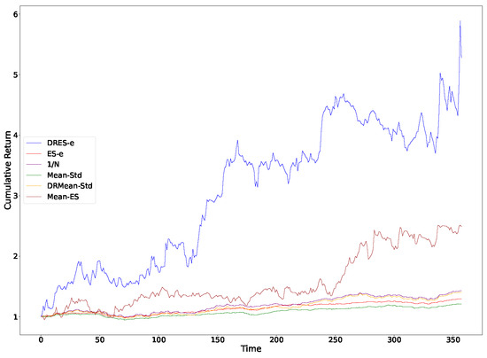
Figure 1.
Cumulative returns of all models with a sliding window of 3.
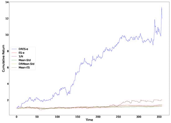
Figure 2.
Cumulative returns of all models with a sliding window of 7.
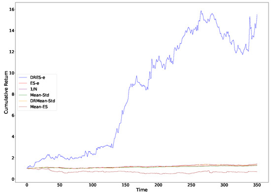
Figure 3.
Cumulative returns of all models with a sliding window of 14.
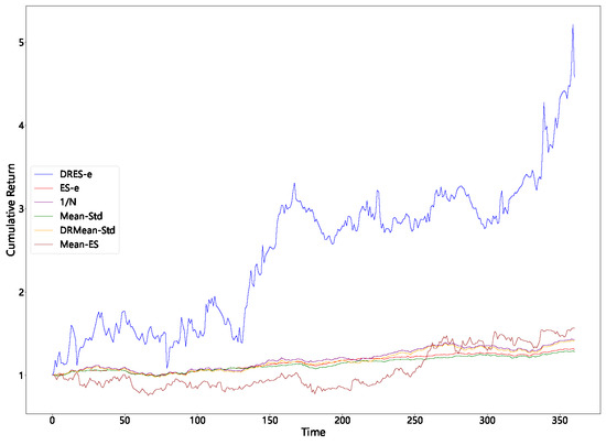
Figure 4.
Cumulative returns of all models with a sliding window of 21.
Furthermore, to explore the reason behind the high average returns of our question, we fix the sliding window to 7, keeping other parameters unchanged. We record the solution vectors for each question at each stage (52 in total, with each solution vector having 130 dimensions, corresponding to 130 stocks), i.e., the portfolio weights. We then calculate the following statistics: the average number of components in the solution vector greater than 0.05, 0.1, and 0.2 and average values of the maximum, minimum, median, 25th percentile, and 5th percentile components of the solution vectors.
As shown in Table 3, and represent the average number of components exceeding 0.05, 0.1, and 0.2, respectively. and represent the average of the maximum value and the median value of the components. As for the 25th percentile, 5th percentile, and minimum value of the components, all are smaller than and are approximately equal to zero within the arithmetic precision; thus, they are not presented or analyzed here.
Table 3.
Statistical summary of the different questions’ solutions.
Based on the five concentration indicators, and , a clear gradient of capital allocation emerges: DRES-expectile attains , , and , meaning that in almost every rolling window the entire budget is staked on a single stock and the remaining 129 weights are truncated to machine precision. This “all-in one bet” design amplifies stock selection skill into explosive portfolio returns whenever the portfolio question correctly pinpoints the short-term winner.
ES-expectile remains highly focused but is less extreme: On average, roughly six stocks exceed the threshold, none exceed , and the largest position is capped at ; together with this delivers a milder risk–return trade-off than DRES-expectile.
Mean-ES lies in between: and show that one to two stocks carry more than each, the largest weight is limited to , and confirms that the long tail is still heavily pruned; the portfolio question therefore preserves high concentration while curbing the tail risk observed with DRES-expectile.
Mean-Std and ES-expectile (under the empirical distribution) display a “barbell” pattern with moderate concentration (, ) and no exposure above , whereas DRMean-Std (G thresholds all zero, , ) spreads the weight almost uniformly across the universe.
Since it is neither realistic nor prudent to invest all the capital in a single stock in typical investment scenarios, we slightly adjust the solution of DRES-expectile by lowering the maximum investment weights to 0.5, 0.3, 0.1, and 0.05, while evenly distributing the remaining weights among the other stocks for data experiments. Additionally, we anticipate that some may question whether we are truly maximizing the expected return, so we also conducted tests to address this. In the following figures and table, we provide a brief explanation of the abbreviations used: DRES-e(50), DRES-e(30), DRES-e(10), and DRES-e(5) represent the results where the maximum investment weights are set to 0.5, 0.3, 0.1, and 0.05, respectively, with the remaining weight evenly distributed. “Mean” represents the solution to the following optimization problem
Table 4 shows that imposing progressively tighter caps on the maximum single-asset weight (from 50% down to 5%) brings a sharp reduction in portfolio variance and expected shortfall, while the corresponding fall in mean return is comparatively small. This characteristic can also be directly observed from Figure 5, Figure 6, Figure 7 and Figure 8. Because volatility declines more rapidly than the mean, the Sharpe and Sortino ratios actually rise, particularly in the 14-day window, which indicates that tail risk in the unconstrained solution is driven chiefly by extreme concentration.
Table 4.
Performance metrics for the improved DRES-expectile solution and mean questions.
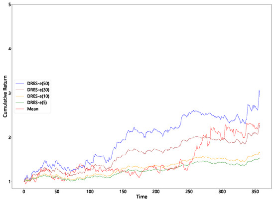
Figure 5.
Cumulative returns with a sliding window of 3 (improved DRES-expectile vs. mean).
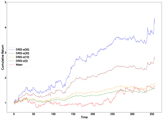
Figure 6.
Cumulative returns with a sliding window of 7 (improved DRES-expectile vs. mean).
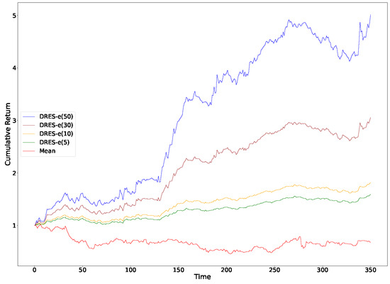
Figure 7.
Cumulative returns with a sliding window of 14 (improved DRES-expectile vs. mean).
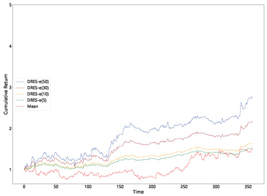
Figure 8.
Cumulative returns with a sliding window of 21 (improved DRES-expectile vs. mean).
The mean-only benchmark produces weaker risk-adjusted results across every horizon and even shows negative average returns in the 14-day window; therefore, our optimization problem cannot be regarded as a simple return maximization exercise. Over the longest window (21 days) the advantage of DRES-expectile narrows, suggesting that its edge is strongest when the portfolio question is recalibrated frequently. We therefore recommend employing the capped DRES-expectile portfolio as a tactical sleeve on short rolling windows, while pairing it with more conservative strategies to stabilize long-term risk.
6. Discussion
In this section, we first examine the practical benefits of measuring portfolio risk using an expectile-based framework augmented with DRES-expectile, from both managerial and investor viewpoints. We then translate our empirical findings into concrete managerial implications for the design of future portfolio optimization strategies, showing how the DRES-expectile portfolio question can be deployed tactically, integrated into multi-strategy architectures, and governed under real-world risk budgets.
6.1. Risk Measurement Implications for Managers and Investors
The numerical experiments presented earlier clearly demonstrate the practical characteristics of the DRES-expectile portfolio question: superior average return and Sharpe ratio across all sliding windows, but accompanied by higher volatility and concentration risk. These results lead to two distinct sets of implications, one for portfolio managers and risk controllers, and one for investors.
6.1.1. Managerial Perspective
Tail-aware and continuously adjustable risk control. In contrast to “threshold-triggered” jump reactions typical of Value-at-Risk portfolio questions, an expectile-based risk metric offers earlier and smoother tail risk warnings. Thanks to this continuity, managers can employ gradient-based optimization to fine-tune risk in real time, greatly improving the controllability and sensitivity of portfolio adjustments.
Practical governance levers. The primary issues—elevated expected shortfall and high volatility—arise from oversized single-stock exposure. A governance committee can remedy this simply by imposing position-weight caps, a standard control tool. Once these caps are in place, the portfolio’s Sharpe ratio still surpasses that of all classical portfolio questions over 3 to 14 day windows, demonstrating that the framework aligns seamlessly with existing risk management policies.
6.1.2. Investor Perspective
Transparent risk–return trade-off. The ES-expectile metric produces a continuous, tail-sensitive spectrum of risk values. This enables investors to see not just how often losses might occur but also how severely, and how this evolves as portfolio positions are adjusted. Unlike threshold-based measures such as VaR, this “risk spectrum” facilitates better understanding and more informed investment decisions.
Downside protection with controlled sacrifice. When upper bounds are applied (DRES-e(30/10/5)), the portfolio question significantly reduces ES while preserving high Sharpe ratios. Investors obtain a more balanced growth path by accepting marginally lower peaks in exchange for markedly lower drawdowns, which is especially desirable for institutions with capital preservation mandates.
6.2. Managerial Implications for Future Portfolio Optimization Strategies
6.2.1. Strategic Application
Across every window length, the DRES-expectile portfolio question shows a strong, steadily rising performance trajectory, whereas traditional portfolio questions produce much flatter curves. Investors thus observe a continuous risk-evolution path and can detect the build-up of potential tail risk sooner, avoiding the VaR-style “risk-silent interval.” This clearer view of the risk–return trade-off empowers investors to make more forward-looking allocation decisions.
For more risk-averse investors, such as pension funds or insurance portfolios, the DRES-expectile portfolio question should be positioned as a satellite strategy—allocated only within clearly defined risk budgets. This approach enables controlled exposure to potential upside while maintaining the portfolio’s overall risk discipline.
6.2.2. Integration with Other Strategies
To further improve long-term portfolio stability, we recommend integrating the DRES-expectile portfolio question into a broader multi-strategy architecture:
- Core satellite structure: Use low-volatility portfolio questions such as mean–variance or minimum variance for the core portfolio, and deploy DRES-expectile as a growth-seeking satellite component.
- Dynamic window adjustment: Vary the sliding window length adaptively based on market volatility or regime shifts, ensuring the portfolio question does not overfit to a fixed horizon.
- Risk budgeting and cap enforcement: Assign explicit volatility or VaR limits to the DRES-expectile sleeve, and coordinate with other sub-strategies to manage overall portfolio risk. This allows total portfolio exposure to remain within pre-defined limits while leveraging the growth potential of the robust tail-aware portfolio question.
7. Conclusions
We first introduced the expectation gap to extend the traditional risk measure and expectile, and demonstrated its effectiveness by proving that it has a solution. To better control the instability caused by empirical distributions, we employed distributionally robust optimization, introduced necessary theorems, and made reasonable assumptions. We then updated the ES-expectile and simplified the problem using optimization techniques. In numerical experiments, our DRES-expectile method almost exactly captured the trend in stock growth, resulting in the selection of only one stock in each decision, which led to excellent returns, though with a higher standard deviation. We acknowledge that such results may seem unrealistic and lack persuasiveness in practical applications. Therefore, we further conducted data experiments to show that this portfolio problem is not simply an expectation maximization problem. Moreover, by adjusting the weight of extreme solutions, we proposed a more practical portfolio strategy. We believe that this portfolio problem has potential when combined with other conservative investment strategies and holds certain reference value and research significance.
Author Contributions
Conceptualization, H.W., Y.Z. and C.L.; methodology, H.W., Y.Z., C.L. and X.Z.; software, H.W. and Y.Z.; validation, H.W., Y.Z., Y.G. and C.L.; formal analysis, Y.G.; investigation, H.W. and Y.G.; resources, Y.Z.; data curation, Y.G.; writing—original draft preparation, H.W., Y.Z., Y.G. and X.Z.; writing—review and editing, H.W., Y.Z., C.L. and X.Z.; visualization, Y.Z.; supervision, H.W. and C.L.; project administration, H.W. and C.L.; funding acquisition, C.L. All authors have read and agreed to the published version of the manuscript.
Funding
This research was funded by the Key Science and Technology Research Project of Henan Province of China OF FUNDER grant number 252102240125.
Data Availability Statement
The stock closing price data used in this study are publicly available at Investing.com (https://cn.investing.com), a widely used financial market platform that provides comprehensive financial data, real-time quotes, charts, and financial news on global stocks, indices, commodities, and currencies.
Conflicts of Interest
The authors declare no conflicts of interest.
References
- Markowitz, H. The utility of wealth. J. Political Econ. 1952, 60, 151–158. [Google Scholar] [CrossRef]
- Chopra, V.K.; Ziemba, W.T. The effect of errors in means, variances, and covariances on optimal portfolio choice. J. Portfolio Manag. 1993, 19, 6–11. [Google Scholar] [CrossRef]
- Cai, J.; Weng, C. Optimal reinsurance with expectile. Scand. Actuar. J. 2016, 2016, 624–645. [Google Scholar] [CrossRef]
- Bellini, F.; Klar, B.; Müller, A.; Rosazza Gianin, E. Generalized quantiles as risk measures. Insur. Math. Econ. 2014, 54, 41–48. [Google Scholar] [CrossRef]
- Zhang, F.; Xu, Y.; Fan, C. Non-parametric inference of expectile-based value-at-risk for financial time series with application to risk assessment. Int. Rev. Financ. Anal. 2023, 90, 102852. [Google Scholar] [CrossRef]
- Taylor, J.W. Estimating value at risk and expected shortfall using expectiles. J. Financ. Econom. 2008, 6, 231–252. [Google Scholar] [CrossRef]
- Rockafellar, R.T.; Uryasev, S. Conditional value-at-risk for general loss distributions. J. Bank. Financ. 2002, 26, 1443–1471. [Google Scholar] [CrossRef]
- Rahimian, H.; Mehrotra, S. Frameworks and results in distributionally robust optimization. Open J. Math. Optim. 2022, 3, 4. [Google Scholar] [CrossRef]
- Mohajerin Esfahani, P.; Kuhn, D. Data-driven distributionally robust optimization using the Wasserstein metric: Performance guarantees and tractable reformulations. Math. Program. 2018, 171, 115–166. [Google Scholar] [CrossRef]
- Gao, R.; Kleywegt, A.J. Distributionally robust stochastic optimization with Wasserstein distance. Math. Oper. Res. 2022, 48, 603–655. [Google Scholar] [CrossRef]
- Gao, R.; Chen, X.; Kleywegt, A.J. Wasserstein distributionally robust optimization and variation regularization. Oper. Res. 2022, 72, 1177–1191. [Google Scholar] [CrossRef]
- Shafieezadeh-Abadeh, S.; Kuhn, D.; Mohajerin Esfahani, P. Regularization via mass transportation. J. Mach. Learn. Res. 2019, 20, 1–68. [Google Scholar]
- Blanchet, J.; Chen, L.; Zhou, X.Y. Distributionally robust mean-variance portfolio selection with Wasserstein distances. Manag. Sci. 2022, 68, 6382–6410. [Google Scholar] [CrossRef]
- Chen, D.; Wu, Y.; Li, J.; Zhou, X. Distributionally robust mean–absolute deviation portfolio optimization using the Wasserstein metric. J. Glob. Optim. 2023, 87, 783–805. [Google Scholar] [CrossRef]
- Liu, W.; Liu, Y. Worst-case higher-moment coherent risk based on optimal transport with application to distributionally robust portfolio optimization. Symmetry 2022, 14, 138. [Google Scholar] [CrossRef]
- Wu, Z.; Sun, K. Distributionally robust optimization with Wasserstein metric for multi-period portfolio selection under uncertainty. Appl. Math. Model. 2023, 117, 513–528. [Google Scholar] [CrossRef]
- Zhang, Z.; Jing, H.; Kao, C. High-dimensional distributionally robust mean-variance efficient portfolio selection. Mathematics 2023, 11, 1272. [Google Scholar] [CrossRef]
- Fan, Z.; Ji, R.; Lejeune, M.A. Distributionally robust portfolio optimization under marginal and copula ambiguity. J. Optim. Theory Appl. 2024, 203, 2870–2907. [Google Scholar] [CrossRef]
- Shapiro, A. On duality theory of conic linear problems. Nonconvex Optim. Appl. 2001, 57, 135–155. [Google Scholar] [CrossRef]
- Chaudhry, A.; Johnson, H.L. The efficacy of the Sortino ratio and other benchmarked performance measures under skewed return distributions. Aust. J. Manag. 2008, 32, 485–502. [Google Scholar] [CrossRef]
- Virtanen, P.; Gommers, R.; Oliphant, T.E.; Haberland, M.; Reddy, T.; Cournapeau, D.; Burovski, E.; Peterson, P.; Weckesser, W.; Bright, J.; et al. SciPy 1.0: Fundamental algorithms for scientific computing in Python. Nat. Methods 2020, 17, 261–272. [Google Scholar] [CrossRef]
Disclaimer/Publisher’s Note: The statements, opinions and data contained in all publications are solely those of the individual author(s) and contributor(s) and not of MDPI and/or the editor(s). MDPI and/or the editor(s) disclaim responsibility for any injury to people or property resulting from any ideas, methods, instructions or products referred to in the content. |
© 2025 by the authors. Licensee MDPI, Basel, Switzerland. This article is an open access article distributed under the terms and conditions of the Creative Commons Attribution (CC BY) license (https://creativecommons.org/licenses/by/4.0/).