Robust Load Frequency Control in Hybrid Microgrids Using Type-3 Fuzzy Logic Under Stochastic Variations

Abstract

This paper presents a type-3 fuzzy logic (T3-FL)-based controller for Load Frequency Control (LFC) in microgrids, focusing on addressing the challenges of renewable energy integration. The integration of renewable sources such as wind and solar leads to power fluctuations and frequency deviations that compromise system stability. The proposed T3-FL controller incorporates advanced features like online adaptation of membership functions and enhanced computational capacity to manage uncertainties in renewable power generation and load variations. The design principles prioritize robustness, adaptability to stochastic variations, and effective frequency stabilization. Simulation results demonstrate that the T3-FL controller significantly improves the microgrid’s stability by efficiently mitigating frequency fluctuations across multiple dynamic scenarios.

1. Introduction

The accelerated growth in technology, in conjunction with the expanding global population, has led to a marked rise in humanity’s reliance on energy resources. Projections indicate that energy consumption will experience a 40% surge by the year 2040 [1,2]. Presently, the energy sector’s reliance on fossil fuels, which are both environmentally detrimental and non-renewable, stands at 7% [3]. In response to these challenges, governments worldwide have implemented policies and incentives aimed at addressing environmental pollution and energy scarcity. For instance, the Chinese government has convened a carbon summit and established carbon neutrality targets for 2020 [4], Furthermore, there has been a growing global call for a transition to renewable energy sources in order to mitigate greenhouse gas emissions caused by fossil fuel consumption [5]. The adverse environmental impact of fossil fuels and energy scarcity has led to a rapid transition to environmentally friendly renewable energy sources (RES) [6]. The integration of RES in power systems has led to a paradigm shift, giving rise to the concept of Microgrid (MG) [7,8]. These Microgrids offer distinct advantages, including their capacity to connect to the interconnected grid or operate autonomously, thereby expanding the scope of MG applications [9].

Depending on the atmospheric conditions, the generation levels of WPPs vary continuously, which leads to power fluctuations and frequency deviations in the system [10,11]. This situation reduces energy efficiency and system stability. To prevent this unfavorable situation, a well-designed load frequency control (LFC) is necessary [12,13,14].

As seen in Figure 1, previous works for LFC can be considered in six main categories: (1) Classical Control Methods; (2) Intelligent Control Approaches; (3) Fuzzy Logic-Based Controllers; (4) Optimization-Based Controllers; (5) Robust/Advanced Control Strategies; (6) Distributed and Artificial Intelligence-Based Controllers.

Classical Control Techniques: Classical controllers such as PID and PI have been widely used for LFC due to their simplicity and ease of implementation. For example, a PID controller for LFC in wind energy systems was explored in [15], where the authors enhanced performance through the construction of a Lyapunov-Krasovskii functional. In [16], PI and PID controllers tuned via an Artificial Rabbit Optimization (ARO) algorithm were developed to manage disturbances in isolated microgrids. However, classical methods tend to exhibit performance degradation under nonlinear conditions and uncertainty, highlighting their limited robustness in modern systems with high renewable penetration.

Intelligent Control Approaches: The increasing integration of stochastic renewable sources has motivated the adoption of intelligent controllers. Ahmed et al. [17] proposed an Integral Derivative-Tilt (ID-T) controller tuned using the Archimedes Optimization Algorithm (AOA), while Abid [18] introduced a cascade coupled derivative-proportional integral (PD-PI) controller optimized with the Enhanced Slime Mold Optimization Algorithm (ESMOA). Long Short-Term Memory (LSTM)-based controllers, as seen in [19], leverage deep learning for predictive frequency control, showcasing superior accuracy over traditional structures. These approaches offer adaptability but often require significant training data and computational resources.

Fuzzy Logic-Based Methods: Fuzzy Logic Controllers (FLCs) have shown great promise for LFC due to their ability to handle system uncertainties and nonlinear dynamics. A genetic algorithm–fuzzy logic (GA-FL) controller was proposed in [20] for a two-area interconnected system demonstrating superior performance to conventional methods. Fractional Order Sliding Mode Control (FOSMC), as introduced in [21], and Interval Type-2 Fuzzy PID (IT2FSs-PID) in [22] further highlight the flexibility and robustness of fuzzy frameworks. In [23], fuzzy logic-based sliding mode control provided effective stabilization, while Ali et al. [24] utilized a genetic algorithm–fuzzy logic self-tuning controller. However, fuzzy-based approaches sometimes suffer from scalability issues and the need for careful rule base and membership function design.

Optimization-Based Hybrid Controllers: A significant body of work has focused on optimization-enhanced controllers for LFC. In [25], a PID controller using Particle Swarm Optimization (PSO) was applied to a system integrating thermal, PV, WTG, and Fuel Cell (FC) units. A more advanced PSO–Artificial Hummingbird Algorithm (PSO-AHA) was proposed in [26] for similar systems. Other hybrid methods include jellyfish search optimization-PID, FOPID, and 2DOF-PID controllers for ship microgrids [27] and advanced equilibrium-optimizer–slime mold algorithms for tuning high-DOF PID variants [28]. Despite their accuracy and flexibility, such approaches may entail high computational burdens and may lack real-time feasibility without hardware acceleration.

Robust and Advanced Control Methods: Robust control strategies, such as the Linear Quadratic Gaussian (LQG) method [29], Linear Matrix Inequality (LMI) controller [30], and H∞-based event-triggered control with dynamic triggering algorithms [31], aim to offer deterministic guarantees of stability and performance. Similarly, Guo [32] introduced adaptive high-order sliding mode control (HOSMC) for oscillation suppression in multi-area systems. Lan and Illindala [30] focused on asymptotic stability in four-area systems, while [33] proposed coordinated emergency controllers for critical load scenarios involving Electrolytic Aluminum Load (EAL). While these techniques offer theoretical robustness, they often require precise system modeling and are sometimes difficult to implement in highly nonlinear or time-varying environments.

Emerging Distributed and AI-Based Approaches: Recent developments have shown increasing interest in distributed and learning-based methods. Li et al. [34] proposed a distributed intelligent coordinated automatic generation control (DI-CAGC) with EIC-MADDPG, a multi-agent deep reinforcement learning strategy. These approaches can autonomously adapt to system variations and optimize control policies, representing a shift toward data-driven solutions in smart grid environments. However, such systems may face limitations in terms of explainability, convergence speed, and validation in hardware-in-the-loop platforms.

In another study, Abdelrahim and Almakhles [35] proposed an event-triggered control strategy for LFC in a hybrid power system containing a WTG, a DG, a BESS, and improved frequency regulation. Their approach differs from the previous studies by incorporating event-triggered control, which ensures that the controller only activates when necessary, thus reducing computational costs. This controller operates in a coordinated fashion to handle emergency conditions, highlighting a significant difference from other controllers that primarily focus on steady-state performance. Other noteworthy contributions include Ekinci et al. [36], who proposed a FOPI(1 + PDN) controller for LFC of a two-area power system comprising PV and thermal generators, which employs the spider wasp optimizer (SWO) for parameter settings. The use of FOPI and SWO in their work sets it apart by focusing on fractional-order control and optimization techniques to achieve more precise parameter tuning. In [37], a neural network-based internal model control (NN-IMC) for LFC in a 75-bus, 15-generator power system is developed and demonstrated to demonstrate robust performance. In [38], Haydaroğlu tests a chaos-based controller for LFC in an airport microgrid with five different scenarios and achieves high performance. However, considering the rapid evolution of control strategies for power systems, it is essential to keep pace with the latest developments, such as those involving Markov Jump System modeling [39] or advanced techniques in weak grid resilience [40], which can offer even greater stability and robustness. These approaches introduce models more attuned to the challenges posed by weak grids and remote areas, which mark a difference from the more conventional control schemes.

Table 1. Summary of literature related to LFC.

Ref.	Controller	Power Source	Working Environment	Advantages	Disadvantages
[41]	adaptive fuzzy	variable speed wind turbine generator	The validation of the method is performed by means of a real-time hardware-in-the-loop (HIL) simulation based on OPAL-RT.	(i) use of fuzzy-based schema (ii) wind turbine stability	(i) Failure to assess the system impacts of other generation sources such as PV
[42]	quadratic differential games theory	PV, BESS, WTG	A Matlab/Simulink model of an islanded microgrid model was created.	(i) Consideration of the operating characteristics of each micro-source (ii) Considering the benefit of all components to realize the coordination arrangement of micro DGs in the microgrid system	(i) This method applies only to the decentralized control method
[43]	Self-tuning-Adaptive fuzzy controller	FW, DG, FC, and WT	Matlab/Simulink model of an islanded microgrid model was created.	(i) Using the artificial bee colony (ABC) algorithm in a fuzzy logic controller to determine the parameters of membership functions based on a multi-objective function	(i) not addressing the stability and oscillation impact of other distributed resources and storage systems
[44]	The stability boundary locus (SBL)	PV/WTG/FC/Electrolyzer/BESS	Matlab/Simulink model of an islanded microgrid model was created.	(i) Use of a fuel cell as a backup generator	(i) frequency distortion when the GPM value exceeds the specified limit in the mathematically based equations.
[45]	two dimensional Sine Logistic map-based chaotic sine cosine algorithm (2D-SLCSCA) optimized classical PID	PV/WTG/FC/FW/BESS/DG and microturbine	Matlab/Simulink model of an islanded microgrid model was created.	(i) The use of an optimized classical PID controller with a two-dimensional Sine Logistic map-based chaotic sine cosine algorithm (2D-SLCSCA)	(i) Power output limitations of MG components such as BESS or DG are not taken into account
[46]	fuzzy fractional sequential PI controller	shipboard MG with PV/FC/FW/BESS	A Matlab/Simulink model of the microgrid model has been created, and the validation of the method is carried out with OPAL-RT-based real-time hardware-in-the-loop (HIL) simulation.	(i) type-2 fuzzy fractional sequential PI (SIT2-FFOPI) controller	(i) The impact of other distributed resources and storage systems on stability and oscillation is not addressed (ii) not addressing the problems of grid-connectedness in different microgrid organizations
[47]	Fuzzy Logic Controller	PV/FC/Electrolyzer/Biodiesel engine generator, Biogaz Turbine Generator	The microgrid model was created in Matlab/Smilunilk model	(i) Cascaded Dual Input Range Type 2 Fuzzy Logic Controller (C-DIT2-FLC)	(i) not using higher-order fuzzy systems
Proposed method	TIP-3 Fuzzy Logic Controller	BESS, FW, DG, FC, PV and WTG	Matlab/Simulink model of an islanded microgrid model was created.	(i) Type-3 FLC, model-independent, no membership function limitation (ii) Considered scholastic variations for wind, solar, and load

presents a range of methods employed in load frequency control, along with a discussion of their respective advantages and disadvantages.

In this paper, we put forth a T3-FLC-based controller for load frequency control in microgrids. This controller boasts a higher computational capacity, which enables it to model complex system dynamics with efficiency. A distinguishing feature of our approach is its incorporation of nonlinearities, a departure from the conventional BPC-based controllers. This adaptability to uncertainties is a key advantage of our method. Furthermore, the controller’s rule base and membership functions are adapted online through the use of accelerated learning algorithms, thus ensuring high performance under varied conditions. The efficacy of the proposed method is substantiated through rigorous experimentation, which encompasses scenarios involving load variations, fluctuations in renewable energy sources, and other dynamic disturbances. This study investigates the performance of the proposed controller when confronted with stochastic variations in wind speed, solar radiation, and load.

The contributions of our work to the literature can be summarized as follows:

• Firstly, although type-1 and type-2 fuzzy logic controllers have been extensively studied in the literature, a type-3 fuzzy logic controlled load frequency control (LFC) mechanism has not been thoroughly investigated in microgrid systems. Our study presents a novel method that utilizes type-3 fuzzy logic to more effectively model uncertainties and enhance system stability.
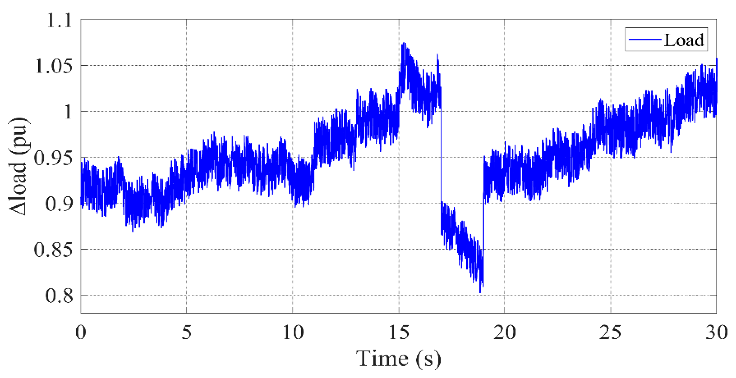
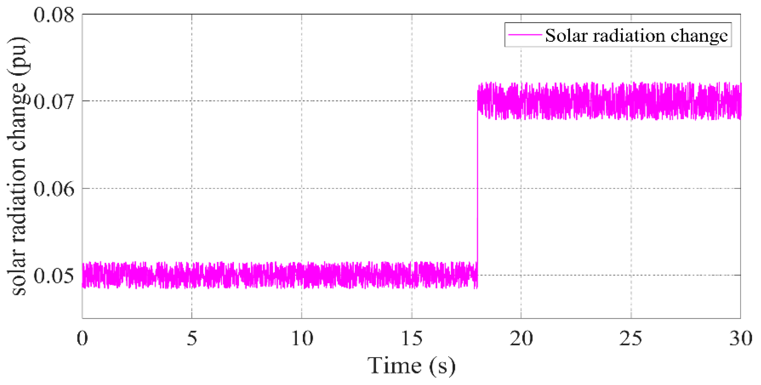
• Furthermore, in contrast to the microgrid analyses in the literature, which are usually performed under deterministic (fixed) conditions, this study allows for stochastic modeling and analysis of wind speed, solar radiation, and load variations, thus contributing to a more comprehensive understanding of the impact of real-world uncertainties on microgrid systems and to the evaluation of the dynamic performance of the system.
• This study involves the testing of various combinations of energy sources and storage systems utilized within the microgrid. This is achieved by analyzing the contributions of BESS, DG, FC, and FW to system stability across five distinct scenarios. Additionally, a comprehensive evaluation of disparate energy management strategies is conducted. This comprehensive approach has the potential to serve as a guide for the selection of system components in future microgrid designs.
• This study also examines the limitations of traditional fuzzy logic methods, which typically have fixed membership functions and are unable to adapt to changing system conditions. Type-3 fuzzy logic addresses this shortcoming by offering a more adaptable approach.
• It is evident that PID-based methods are incapable of sufficiently dampening frequency fluctuations. The proposed controller, however, exhibits a superior capacity to suppress such deviations due to its adaptive nature.

The remainder of this paper is structured as follows. Section 2.1 encompasses microgrid load frequency modeling. Section 2.2 focuses on the TIP-3 FLC, and Section 2.3 focuses on wind power, photovoltaic, and load uncertainty modeling. Section 3 presents the simulation and results, and the conclusion is presented in Section 4.

2. Materials and Methods

2.1. Microgrid Model

In recent years, a marked tendency toward the use of renewable energy sources, as opposed to more traditional sources, which are considered to cause harm to the natural environment, has become increasingly apparent. As a result of this shift in focus, microgrids have begun to assume a greater significance. The deployment of various Distributed Energy Resources (DERs) in microgrids (MCs) is determined by many factors, including the design and operating principles of the particular microgrid, as well as the technology generation used by the DERs. Renewable energy sources, such as wind turbine generators (WTG) and photovoltaic systems (PV), as well as conventional energy sources, including diesel generators (DG), are included in DERs. The production of intermittent energy sources, such as WTG and PV, cannot be directly controlled. Therefore, a reliable generator system, such as DG, can play a critical role in improving reliability. Fuel cells (FC) are also one of the commonly used power generation units in microgrids. This study proposes a microgrid model integrating diverse generation and storage sources, including WTG, PV, battery energy storage systems (BESS), flywheel (FW), diesel generators (DG), and fuel cells (FC) [48]. The proposed microgrid model is depicted in Figure 2 and has been simulated using MATLAB/Simulink.

The system parameters are provided in

Table 2. Parameters for the microgrid model.

Parameter	Value	Parameter	Value
${\mathit{T}}_{\mathit{W}\mathit{T}\mathit{G}}$	1.5	${\mathit{T}}_{\mathit{D}\mathit{G},\mathit{T}\mathit{g}}$	0.08
${\mathit{T}}_{\mathit{F}\mathit{W}}$	0.1	${\mathit{T}}_{\mathit{D}\mathit{G},\mathit{T}\mathit{t}}$	0.4
${\mathit{T}}_{\mathit{B}\mathit{E}\mathit{S}\mathit{S}}$	0.1	${\mathit{T}}_{\mathit{M}\mathit{G}}$	0.1667
${\mathit{T}}_{\mathit{P}\mathit{V}\_\mathit{i}\mathit{n}\mathit{v}}$	0.04	${\mathit{K}}_{\mathit{M}\mathit{G}}$	0.0015
${\mathit{T}}_{\mathit{P}\mathit{V}\_(\mathit{l}/\mathit{c})}$	0.004	${\mathit{T}}_{\mathit{F}\mathit{C},\mathit{t}\mathit{c}}$	0.26
${\mathit{T}}_{\mathit{F}\mathit{C}\_(\mathit{l}/\mathit{c})}$	0.004	${\mathit{T}}_{\mathit{F}\mathit{C}\_\mathit{i}\mathit{n}\mathit{v}}$	0.04

.

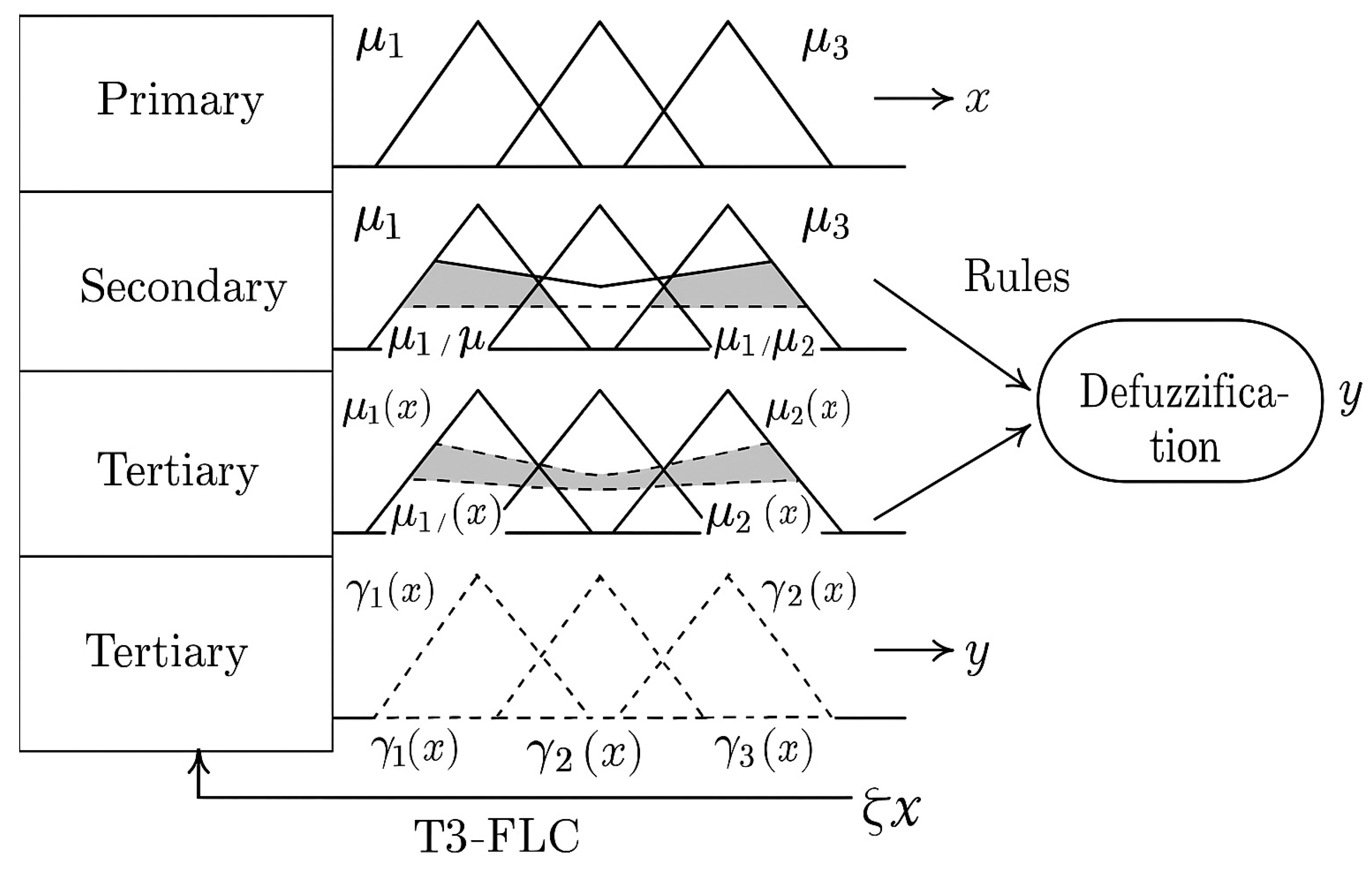
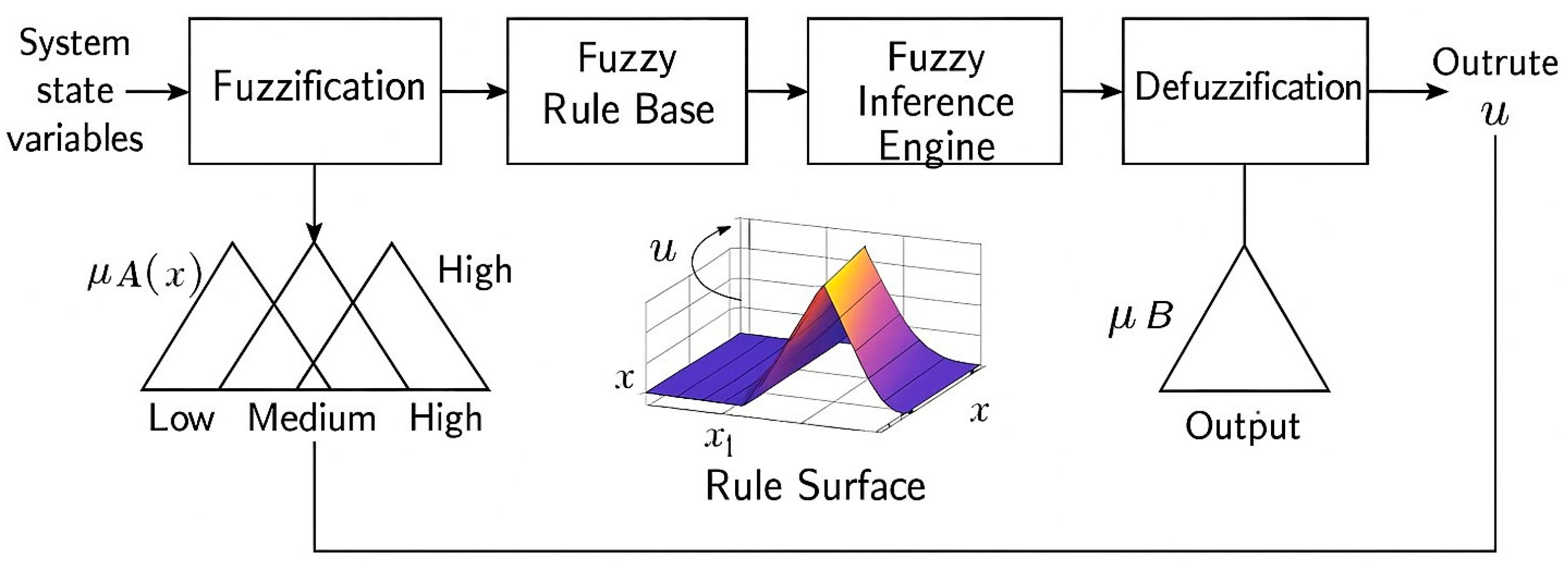
2.2. Type3 Fuzzy Logic Controller

Introduced in 1965 by Zadeth, Fuzzy Logic (FL) [49] is a control algorithm that processes input data with precise values and produces outputs with precise values. The important criterion in all methods based on fuzzy logic is that the input values are set correctly and accurately; that is to say, the previous values of voltage and frequency must be determined. This is because, when fluctuation occurs, the system can intervene by saving the previous values in its memory. In the field of control theory, type-1 fuzzy logic control (T1-FLC) and type-2 fuzzy logic control (T2-FLC) methods have emerged as the predominant approaches. Traditional type-1 fuzzy logic control systems are characterized by precise rules, which are typically based on specific operating conditions and define the desired output. In contrast, type-2 fuzzy logic control can address more complex conditions; however, T3-FLC offers a superior level of flexibility for voltage and frequency control in microgrid systems by addressing the levels of uncertainty within the system from a broader perspective. T3-FLC can rapidly adapt to dynamic and sudden changes in microgrid systems [50,51]. The present paper proposes a type-3 fuzzy logic control (T3-FLC) method for load-frequency control of microgrids. For a more detailed analysis of the method, readers are directed to Equations (1)–(59), which are discussed in detail. In Equations (1) and (2), h is the error of the controlled parameter, ${\mathit{S}}_{\mathit{a}}^{\mathit{b}}\mathit{h} \mathit{a}\mathit{n}\mathit{d} {\mathit{K}}_{\mathit{a}}^{\mathit{b}}\mathit{h}$, h are the operations on this error. z is the error value occurring in different sections [52].

$${\mathit{S}}_{\mathit{a}}^{\mathit{b}}\mathit{h}\left(\mathit{a}\right)={\displaystyle \frac{{\int }_{\mathbf{0}}^{\mathit{a}}\mathit{h}\left(\mathit{z}\right){\left(\mathit{a}-\mathit{z}\right)}^{-\mathit{b}}\mathit{d}\mathit{z}}{\mathsf{\delta }\left(\mathbf{1}-\mathit{b}\right)}}$$

(1)

$${\mathit{K}}_{\mathit{a}}^{\mathit{b}}\mathit{h}\left(\mathit{a}\right)={\displaystyle \frac{{\int }_{\mathbf{0}}^{\mathit{a}}\mathit{h}\left(\mathit{z}\right){\left(\mathit{a}-\mathit{z}\right)}^{\mathit{b}-\mathbf{1}}\mathit{d}\mathit{z}}{\mathsf{\delta }\left(\mathit{b}\right)}}$$

(2)

The membership functions ${\tilde{\mathit{R}}}_{\mathit{n}}^{\mathbf{1}}-{\tilde{\mathit{R}}}_{\mathit{n}}^{\mathbf{2}}$, ${\mathit{R}}_{{\mathit{K}}_{\mathit{a}}^{\mathit{b}}\mathit{h}}^{\mathbf{1}}-{\tilde{\mathit{R}}}_{{\mathit{K}}_{\mathit{a}}^{\mathit{b}}\mathit{h}}^{\mathbf{2}},$ and ${\mathit{R}}_{{\mathit{S}}_{\mathit{a}}^{\mathit{b}}\mathit{h}}^{\mathbf{1}}-{\tilde{\mathit{R}}}_{{\mathit{S}}_{\mathit{a}}^{\mathit{b}}\mathit{h}}^{\mathbf{2}}$ can be regarded as references for the input values h, ${\mathit{S}}_{\mathit{a}}^{\mathit{b}}\mathit{h} \mathit{a}\mathit{n}\mathit{d} {\mathit{K}}_{\mathit{a}}^{\mathit{b}}\mathit{h}$. In the following equations, the functions are divided into specific components to facilitate a more comprehensive analysis of the membership functions. Errors or minor deviations may be encountered in the sensors utilized in the circuits. These errors are calculated in the equations presented in Equations (3)–(6). In these equations, the ${\mathit{\alpha }}_{\mathit{q}}$ value is calculated for each partition:

$${\overline{\mathit{r}}}_{{\tilde{\mathit{R}}}_{\mathit{h}}^{\mathit{y}}|{\overline{\mathit{\alpha }}}_{\mathit{q}}}=\mathit{exp}\left(-{\displaystyle \frac{{\left({\mathit{h}}_{{\overline{\mathsf{\alpha }}}_{\mathit{q}}}-{\mathit{c}}_{{\tilde{\mathit{R}}}_{\mathit{h}}^{\mathit{y}}|{\overline{\mathsf{\alpha }}}_{\mathit{q}}}\right)}^{\mathbf{2}}}{{\overline{\mathit{\vartheta }}}_{{\tilde{\mathit{R}}}_{\mathit{h}}^{\mathit{y}}|{\overline{\mathsf{\alpha }}}_{\mathit{q}}}^{\mathbf{2}}}}\right)$$

(3)

$${\overline{\mathit{r}}}_{{\tilde{\mathit{R}}}_{\mathit{h}}^{\mathit{y}}|{\underset{\_}{\mathsf{\alpha }}}_{\mathit{q}}}=\mathit{exp}\left(-{\displaystyle \frac{{\left({\overline{\mathit{h}}}_{{\underset{\_}{\mathsf{\alpha }}}_{\mathit{q}}}-{\mathit{c}}_{{\tilde{\mathit{R}}}_{\mathit{h}}^{\mathit{y}}|{\underset{\_}{\mathsf{\alpha }}}_{\mathit{q}}}\right)}^{\mathbf{2}}}{{\overline{\mathit{\vartheta }}}_{{\tilde{\mathit{R}}}_{\mathit{h}}^{\mathit{y}}|{\underset{\_}{\mathsf{\alpha }}}_{\mathit{q}}}^{\mathbf{2}}}}\right)$$

(4)

$${\underset{\_}{\mathit{r}}}_{{\tilde{\mathit{R}}}_{\mathit{h}}^{\mathit{y}}|{\overline{\mathsf{\alpha }}}_{\mathit{q}}}=\mathit{exp}\left(-{\displaystyle \frac{{\left({\underset{\_}{\mathit{h}}}_{{\overline{\mathsf{\alpha }}}_{\mathit{q}}}-{\mathit{c}}_{{\tilde{\mathit{R}}}_{\mathit{h}}^{\mathit{y}}|{\overline{\mathsf{\alpha }}}_{\mathit{q}}}\right)}^{\mathbf{2}}}{{\underset{\_}{\mathit{\vartheta }}}_{{\tilde{\mathit{R}}}_{\mathit{h}}^{\mathit{y}}|{\overline{\mathsf{\alpha }}}_{\mathit{q}}}^{\mathbf{2}}}}\right)$$

(5)

$${\underset{\_}{\mathit{r}}}_{{\tilde{\mathit{R}}}_{\mathit{h}}^{\mathit{y}}|{\underset{\_}{\mathsf{\alpha }}}_{\mathit{q}}}=\mathit{exp}\left(-{\displaystyle \frac{{\left({\underset{\_}{\mathit{h}}}_{{\underset{\_}{\mathsf{\alpha }}}_{\mathit{q}}}-{\mathit{c}}_{{\tilde{\mathit{R}}}_{\mathit{h}}^{\mathit{y}}|{\underset{\_}{\mathsf{\alpha }}}_{\mathit{q}}}\right)}^{\mathbf{2}}}{{\underset{\_}{\mathit{\vartheta }}}_{{\tilde{\mathit{R}}}_{\mathit{h}}^{\mathit{y}}|{\underset{\_}{\mathsf{\alpha }}}_{\mathit{q}}}^{\mathbf{2}}}}\right)$$

(6)

The purpose of calculating these equations is twofold: firstly, to eliminate the error values h entering the system, and secondly, to perform some simplification operations on the variables. Following these operations, the equations in Equations (7)–(10) are obtained.

$${\overline{\mathit{r}}}_{{\overline{\mathit{\alpha }}}_{\mathit{q}}}={\displaystyle \frac{{\mathit{h}\overline{\mathit{\vartheta }}}_{{\tilde{\mathit{R}}}_{\mathit{h}}^{\mathit{y}}|{\overline{\mathit{\alpha }}}_{\mathit{q}}}^{\mathbf{2}}+{\mathsf{\gamma }}_{\mathit{s}}^{\mathbf{2}}{\mathit{c}}_{{\tilde{\mathit{R}}}_{\mathit{h}}^{\mathit{y}}|{\overline{\mathit{\alpha }}}_{\mathit{q}}}}{{\overline{\mathit{\vartheta }}}_{{\tilde{\mathit{R}}}_{\mathit{h}}^{\mathit{y}}|{\overline{\mathit{\alpha }}}_{\mathit{q}}}^{\mathbf{2}}+{\mathsf{\gamma }}_{\mathit{s}}^{\mathbf{2}}}}$$

(7)

$${\overline{\mathit{r}}}_{{\underset{\_}{\mathit{\alpha }}}_{\mathit{q}}}={\displaystyle \frac{{\mathit{h}\overline{\mathit{\vartheta }}}_{{\tilde{\mathit{R}}}_{\mathit{h}}^{\mathit{y}}|{\underset{\_}{\mathit{\alpha }}}_{\mathit{q}}}^{\mathbf{2}}+{\mathsf{\gamma }}_{\mathit{s}}^{\mathbf{2}}{\mathit{c}}_{{\tilde{\mathit{R}}}_{\mathit{h}}^{\mathit{y}}|{\underset{\_}{\mathit{\alpha }}}_{\mathit{q}}}}{{\overline{\mathit{\vartheta }}}_{{\tilde{\mathit{R}}}_{\mathit{h}}^{\mathit{y}}|{\underset{\_}{\mathit{\alpha }}}_{\mathit{q}}}^{\mathbf{2}}+{\mathsf{\gamma }}_{\mathit{s}}^{\mathbf{2}}}}$$

(8)

$${\underset{\_}{\mathit{r}}}_{{\overline{\mathit{\alpha }}}_{\mathit{q}}}={\displaystyle \frac{\mathit{h}{\underset{\_}{\mathit{\vartheta }}}_{{\tilde{\mathit{R}}}_{\mathit{h}}^{\mathit{y}}|{\overline{\mathit{\alpha }}}_{\mathit{q}}}^{\mathbf{2}}+{\mathsf{\gamma }}_{\mathit{s}}^{\mathbf{2}}{\mathit{c}}_{{\tilde{\mathit{R}}}_{\mathit{h}}^{\mathit{y}}|{\overline{\mathit{\alpha }}}_{\mathit{q}}}}{{\underset{\_}{\mathit{\vartheta }}}_{{\tilde{\mathit{R}}}_{\mathit{h}}^{\mathit{y}}|{\overline{\mathit{\alpha }}}_{\mathit{q}}}^{\mathbf{2}}+{\mathsf{\gamma }}_{\mathit{s}}^{\mathbf{2}}}}$$

(9)

$${\underset{\_}{\mathit{r}}}_{{\overline{\mathit{\alpha }}}_{\mathit{q}}}={\displaystyle \frac{\mathit{h}{\underset{\_}{\mathit{\vartheta }}}_{{\tilde{\mathit{R}}}_{\mathit{h}}^{\mathit{y}}|{\overline{\mathit{\alpha }}}_{\mathit{q}}}^{\mathbf{2}}+{\mathsf{\gamma }}_{\mathit{s}}^{\mathbf{2}}{\mathit{c}}_{{\tilde{\mathit{R}}}_{\mathit{h}}^{\mathit{y}}|{\overline{\mathit{\alpha }}}_{\mathit{q}}}}{{\underset{\_}{\mathit{\vartheta }}}_{{\tilde{\mathit{R}}}_{\mathit{h}}^{\mathit{y}}|{\overline{\mathit{\alpha }}}_{\mathit{q}}}^{\mathbf{2}}+{\mathsf{\gamma }}_{\mathit{s}}^{\mathbf{2}}}}$$

(10)

In this system, q and y represent the center values, which are regarded as the standard values for ${\overline{\mathit{\vartheta }}}_{{\tilde{\mathit{R}}}_{\mathit{h}}^{\mathit{y}}|{\overline{\mathit{\alpha }}}_{\mathit{q}}},{\underset{\_}{\mathit{\vartheta }}}_{{\tilde{\mathit{R}}}_{\mathit{h}}^{\mathit{y}}|{\overline{\mathit{\alpha }}}_{\mathit{q}}}.$ The value ${\tilde{\mathit{R}}}_{\mathit{h}}^{\mathit{y}}|{\overline{\mathit{\alpha }}}_{\mathit{q}}$ is defined as the membership function within the system. The following equations present the system input value ${\mathit{K}}_{\mathit{a}}^{\mathit{b}}\mathit{h}$: Equations (11)–(14).

$${\overline{\mathit{r}}}_{{\tilde{\mathit{R}}}_{{\mathit{K}}_{\mathit{a}}^{\mathit{b}}\mathit{h}}^{\mathit{y}}|{\overline{\mathit{\alpha }}}_{\mathit{q}}}=\mathit{exp}\left(-{\displaystyle \frac{{\left({\mathit{K}}_{\mathit{a}}^{\mathit{b}}{\overline{\mathit{h}}}_{{\overline{\mathit{\alpha }}}_{\mathit{q}}}-{\mathit{c}}_{{\tilde{\mathit{R}}}_{{\mathit{K}}_{\mathit{a}}^{\mathit{b}}\mathit{h}}^{\mathit{y}}|{\overline{\mathit{\alpha }}}_{\mathit{q}}}\right)}^{\mathbf{2}}}{{\overline{\mathit{\vartheta }}}_{{\tilde{\mathit{R}}}_{{\mathit{K}}_{\mathit{a}}^{\mathit{b}}\mathit{h}}^{\mathit{y}}|{\overline{\mathit{\alpha }}}_{\mathit{q}}}^{\mathbf{2}}}}\right)$$

(11)

$${\overline{\mathit{r}}}_{{\tilde{\mathit{R}}}_{{\mathit{K}}_{\mathit{a}}^{\mathit{b}}\mathit{h}}^{\mathit{y}}|{\underset{\_}{\mathit{\alpha }}}_{\mathit{q}}}=\mathit{exp}\left(-{\displaystyle \frac{{\left({\mathit{K}}_{\mathit{a}}^{\mathit{b}}{\overline{\mathit{h}}}_{{\underset{\_}{\mathit{\alpha }}}_{\mathit{q}}}-{\mathit{c}}_{{\tilde{\mathit{R}}}_{{\mathit{K}}_{\mathit{a}}^{\mathit{b}}\mathit{h}}^{\mathit{y}}|{\underset{\_}{\mathit{\alpha }}}_{\mathit{q}}}\right)}^{\mathbf{2}}}{{\overline{\mathit{\vartheta }}}_{{\tilde{\mathit{R}}}_{{\mathit{K}}_{\mathit{a}}^{\mathit{b}}\mathit{h}}^{\mathit{y}}|{\underset{\_}{\mathit{\alpha }}}_{\mathit{q}}}^{\mathbf{2}}}}\right)$$

(12)

$${\underset{\_}{\mathit{r}}}_{{\mathit{R}}_{{\mathit{K}}_{\mathit{a}}^{\mathit{b}}\mathit{n}}^{\mathit{y}}|{\overline{\mathit{\alpha }}}_{\mathit{q}}}=\mathit{exp}\left(-{\displaystyle \frac{{\left({\mathit{K}}_{\mathit{a}}^{\mathit{b}}{\underset{\_}{\mathit{h}}}_{{\overline{\mathit{\alpha }}}_{\mathit{q}}}-{\mathit{c}}_{{\tilde{\mathit{R}}}_{{\mathit{K}}_{\mathit{a}}^{\mathit{b}}\mathit{h}}^{\mathit{m}}|{\overline{\mathit{\alpha }}}_{\mathit{q}}}\right)}^{\mathbf{2}}}{{\underset{\_}{\mathit{\vartheta }}}_{{\tilde{\mathit{R}}}_{{\mathit{K}}_{\mathit{a}}^{\mathit{b}}\mathit{h}}^{\mathit{y}}|{\overline{\mathit{\alpha }}}_{\mathit{q}}}^{\mathbf{2}}}}\right)$$

(13)

$${\underset{\_}{\mathit{r}}}_{{\tilde{\mathit{R}}}_{{\mathit{K}}_{\mathit{a}}^{\mathit{b}}\mathit{h}}^{\mathit{y}}|{\underset{\_}{\mathit{\alpha }}}_{\mathit{q}}}=\mathit{exp}\left(-{\displaystyle \frac{{\left({\mathit{K}}_{\mathit{a}}^{\mathit{b}}{\underset{\_}{\mathit{h}}}_{{\underset{\_}{\mathit{\alpha }}}_{\mathit{q}}}-{\mathit{c}}_{{\tilde{\mathit{R}}}_{{\mathit{K}}_{\mathit{a}}^{\mathit{b}}\mathit{h}}^{\mathit{y}}|{\underset{\_}{\mathit{\alpha }}}_{\mathit{q}}}\right)}^{\mathbf{2}}}{{\underset{\_}{\mathit{\vartheta }}}_{{\tilde{\mathit{R}}}_{{\mathit{K}}_{\mathit{a}}^{\mathit{b}}\mathit{h}}^{\mathit{y}}|{\underset{\_}{\mathit{\alpha }}}_{\mathit{q}}}^{\mathbf{2}}}}\right)$$

(14)

The objective of these operations is to facilitate the input ${\mathit{K}}_{\mathit{a}}^{\mathit{b}}\mathit{h}$ to operate on the error value h. This process constitutes a simplification of the values of ${\mathit{K}}_{\mathit{a}}^{\mathit{b}}\mathit{h}$. Consequently, the resulting equations in Equations (15)–(18) are as follows:

$${\mathit{K}}_{\mathit{a}}^{\mathit{b}}{\overline{\mathit{h}}}_{{\overline{\mathit{\alpha }}}_{\mathit{q}}}={\displaystyle \frac{{\mathit{K}}_{\mathit{a}}^{\mathit{b}}\mathit{h}{\overline{\mathit{\vartheta }}}_{{\tilde{\mathit{R}}}_{\mathit{h}}^{\mathit{y}}|{\overline{\mathit{\alpha }}}_{\mathit{q}}}^{\mathbf{2}}+{\mathsf{\gamma }}_{\mathit{s}}^{\mathbf{2}}{\mathit{c}}_{{\tilde{\mathit{R}}}_{\mathit{h}}^{\mathit{y}}|{\overline{\mathit{\alpha }}}_{\mathit{q}}}}{{\overline{\mathit{\vartheta }}}_{{\tilde{\mathit{R}}}_{\mathit{h}}^{\mathit{y}}|{\overline{\mathit{\alpha }}}_{\mathit{q}}}^{\mathbf{2}}+{\mathsf{\gamma }}_{\mathit{s}}^{\mathbf{2}}}}$$

(15)

$${\mathit{K}}_{\mathit{a}}^{\mathit{b}}{\overline{\mathit{h}}}_{{\underset{\_}{\mathit{\alpha }}}_{\mathit{q}}}={\displaystyle \frac{{\mathit{K}}_{\mathit{a}}^{\mathit{b}}\mathit{h}{\overline{\mathit{\vartheta }}}_{{\tilde{\mathit{R}}}_{\mathit{h}}^{\mathit{y}}|{\underset{\_}{\mathit{\alpha }}}_{\mathit{q}}}^{\mathbf{2}}+{\mathsf{\gamma }}_{\mathit{s}}^{\mathbf{2}}{\mathit{c}}_{{\tilde{\mathit{R}}}_{\mathit{h}}^{\mathit{y}}|{\underset{\_}{\mathit{\alpha }}}_{\mathit{q}}}}{{\overline{\mathit{\vartheta }}}_{{\tilde{\mathit{R}}}_{\mathit{h}}^{\mathit{y}}|{\underset{\_}{\mathit{\alpha }}}_{\mathit{q}}}^{\mathbf{2}}+{\mathsf{\gamma }}_{\mathit{s}}^{\mathbf{2}}}}$$

(16)

$${\mathit{K}}_{\mathit{a}}^{\mathit{b}}{\underset{\_}{\mathit{h}}}_{{\overline{\mathit{\alpha }}}_{\mathit{q}}}={\displaystyle \frac{{\mathit{K}}_{\mathit{a}}^{\mathit{b}}\mathit{h}{\underset{\_}{\mathit{\vartheta }}}_{{\tilde{\mathit{R}}}_{\mathit{h}}^{\mathit{y}}|{\overline{\mathit{\alpha }}}_{\mathit{q}}}^{\mathbf{2}}+{\mathsf{\gamma }}_{\mathit{s}}^{\mathbf{2}}{\mathit{c}}_{{\tilde{\mathit{R}}}_{\mathit{h}}^{\mathit{y}}|{\overline{\mathit{\alpha }}}_{\mathit{q}}}}{{\underset{\_}{\mathit{\vartheta }}}_{{\tilde{\mathit{R}}}_{\mathit{h}}^{\mathit{y}}|{\overline{\mathit{\alpha }}}_{\mathit{q}}}^{\mathbf{2}}+{\mathsf{\gamma }}_{\mathit{s}}^{\mathbf{2}}}}$$

(17)

$${\mathit{K}}_{\mathit{a}}^{\mathit{b}}{\underset{\_}{\mathit{h}}}_{{\underset{\_}{\mathit{\alpha }}}_{\mathit{q}}}={\displaystyle \frac{{\mathit{K}}_{\mathit{a}}^{\mathit{b}}\mathit{h}{\underset{\_}{\mathit{\vartheta }}}_{{\tilde{\mathit{R}}}_{\mathit{h}}^{\mathit{y}}|{\underset{\_}{\mathit{\alpha }}}_{\mathit{q}}}^{\mathbf{2}}+{\mathsf{\gamma }}_{\mathit{s}}^{\mathbf{2}}{\mathit{c}}_{{\tilde{\mathit{R}}}_{\mathit{h}}^{\mathit{y}}|{\underset{\_}{\mathit{\alpha }}}_{\mathit{q}}}}{{\underset{\_}{\mathit{\vartheta }}}_{{\tilde{\mathit{R}}}_{\mathit{h}}^{\mathit{y}}|{\underset{\_}{\mathit{\alpha }}}_{\mathit{q}}}^{\mathbf{2}}+{\mathsf{\gamma }}_{\mathit{s}}^{\mathbf{2}}}}$$

(18)

As demonstrated in the aforementioned equations, ${\overline{\mathit{\vartheta }}}_{{\tilde{\mathit{R}}}_{{\mathit{K}}_{\mathit{a}}^{\mathit{b}}\mathit{h}}^{\mathit{y}}|{\overline{\mathit{\alpha }}}_{\mathit{q}}}\mathit{v}\mathit{e}{\underset{\_}{\mathit{\vartheta }}}_{{\tilde{\mathit{R}}}_{{\mathit{K}}_{\mathit{a}}^{\mathit{b}}\mathit{h}}^{\mathit{y}}|{\overline{\mathit{\alpha }}}_{\mathit{q}}}$ denote the standard values of the membership function, whilst q and y represent the central values. The value of ${\tilde{\mathit{R}}}_{{\mathit{K}}_{\mathit{a}}^{\mathit{b}}\mathit{h}}^{\mathit{y}}|{\overline{\mathit{\alpha }}}_{\mathit{q}}$ is the membership function in the system, and the equations for the input value ${\mathit{S}}_{\mathit{a}}^{\mathit{b}}\mathit{h}$ are given in Equations (19)–(22) as follows

$${\overline{\mathit{r}}}_{{\tilde{\mathit{R}}}_{{\mathit{S}}_{\mathit{a}}^{\mathit{b}}\mathit{h}}^{\mathit{y}}|{\overline{\mathit{\alpha }}}_{\mathit{q}}}=\mathit{exp}\left(-{\displaystyle \frac{{\left({\mathit{S}}_{\mathit{a}}^{\mathit{b}}{\overline{\mathit{h}}}_{{\overline{\mathsf{\alpha }}}_{\mathit{q}}}-{\mathit{c}}_{{\tilde{\mathit{R}}}_{{\mathit{S}}_{\mathit{a}}^{\mathit{b}}\mathit{h}}^{\mathit{y}}|{\overline{\mathsf{\alpha }}}_{\mathit{q}}}\right)}^{\mathbf{2}}}{{\overline{\mathit{\vartheta }}}_{{\tilde{\mathit{R}}}_{{\mathit{S}}_{\mathit{a}}^{\mathit{b}}\mathit{h}}^{\mathit{y}}|{\overline{\mathsf{\alpha }}}_{\mathit{q}}}^{\mathbf{2}}}}\right)$$

(19)

$${\overline{\mathit{r}}}_{{\tilde{\mathit{R}}}_{{\mathit{S}}_{\mathit{a}}^{\mathit{b}}\mathit{h}}^{\mathit{y}}|{\underset{\_}{\mathit{\alpha }}}_{\mathit{q}}}=\mathit{exp}\left(-{\displaystyle \frac{{\left({\mathit{S}}_{\mathit{a}}^{\mathit{b}}{\overline{\mathit{h}}}_{{\underset{\_}{\mathsf{\alpha }}}_{\mathit{q}}}-{\mathit{c}}_{{\tilde{\mathit{R}}}_{{\mathit{S}}_{\mathit{a}}^{\mathit{b}}\mathit{h}}^{\mathit{y}}|{\underset{\_}{\mathsf{\alpha }}}_{\mathit{q}}}\right)}^{\mathbf{2}}}{{\overline{\mathit{\vartheta }}}_{{\tilde{\mathit{R}}}_{{\mathit{S}}_{\mathit{a}}^{\mathit{b}}\mathit{h}}^{\mathit{y}}|{\underset{\_}{\mathsf{\alpha }}}_{\mathit{q}}}^{\mathbf{2}}}}\right)$$

(20)

$${\underset{\_}{\mathit{r}}}_{{\tilde{\mathit{R}}}_{{\mathit{S}}_{\mathit{a}}^{\mathit{b}}\mathit{h}}^{\mathit{y}}|{\overline{\mathit{\alpha }}}_{\mathit{q}}}=\mathit{exp}\left(-{\displaystyle \frac{{\left({\mathit{S}}_{\mathit{a}}^{\mathit{b}}{\underset{\_}{\mathit{h}}}_{{\overline{\mathsf{\alpha }}}_{\mathit{q}}}-{\mathit{c}}_{{\tilde{\mathit{R}}}_{{\mathit{S}}_{\mathit{a}}^{\mathit{b}}\mathit{h}}^{\mathit{y}}|{\overline{\mathsf{\alpha }}}_{\mathit{q}}}\right)}^{\mathbf{2}}}{{\underset{\_}{\mathit{\vartheta }}}_{{\tilde{\mathit{R}}}_{{\mathit{S}}_{\mathit{a}}^{\mathit{b}}\mathit{h}}^{\mathit{y}}|{\overline{\mathsf{\alpha }}}_{\mathit{q}}}^{\mathbf{2}}}}\right)$$

(21)

$${\underset{\_}{\mathit{r}}}_{{\tilde{\mathit{R}}}_{{\mathit{S}}_{\mathit{a}}^{\mathit{b}}\mathit{h}}^{\mathit{y}}|{\underset{\_}{\mathit{\alpha }}}_{\mathit{q}}}=\mathit{exp}\left(-{\displaystyle \frac{{\left({\mathit{S}}_{\mathit{a}}^{\mathit{b}}{\underset{\_}{\mathit{h}}}_{{\underset{\_}{\mathsf{\alpha }}}_{\mathit{q}}}-{\mathit{c}}_{{\tilde{\mathit{R}}}_{{\mathit{S}}_{\mathit{a}}^{\mathit{b}}\mathit{h}}^{\mathit{y}}|{\underset{\_}{\mathsf{\alpha }}}_{\mathit{q}}}\right)}^{\mathbf{2}}}{{\underset{\_}{\mathit{\vartheta }}}_{{\tilde{\mathit{R}}}_{{\mathit{S}}_{\mathit{a}}^{\mathit{b}}\mathit{h}}^{\mathit{y}}|{\underset{\_}{\mathsf{\alpha }}}_{\mathit{q}}}^{\mathbf{2}}}}\right)$$

(22)

The objective of these operations is to simplify the values of ${\mathit{K}}_{\mathit{a}}^{\mathit{b}}\mathit{h}$ so that the input ${\mathit{S}}_{\mathit{a}}^{\mathit{b}}\mathit{h}$ can operate on the error value h. The resulting equations are as outlined in Equations (23)–(26).

$${\mathit{S}}_{\mathit{a}}^{\mathit{b}}{\overline{\mathit{h}}}_{{\overline{\mathit{\alpha }}}_{\mathit{q}}}={\displaystyle \frac{{\mathit{S}}_{\mathit{a}}^{\mathit{b}}\mathit{h}{\overline{\mathit{\vartheta }}}_{{\tilde{\mathit{R}}}_{\mathit{h}}^{\mathit{y}}|{\overline{\mathsf{\alpha }}}_{\mathit{q}}}^{\mathbf{2}}+{\mathsf{\gamma }}_{\mathit{s}}^{\mathbf{2}}{\mathit{c}}_{{\tilde{\mathit{R}}}_{\mathit{h}}^{\mathit{y}}|{\overline{\mathsf{\alpha }}}_{\mathit{q}}}}{{\overline{\mathit{\vartheta }}}_{{\tilde{\mathit{R}}}_{\mathit{h}}^{\mathit{y}}|{\overline{\mathsf{\alpha }}}_{\mathit{q}}}^{\mathbf{2}}+{\mathsf{\gamma }}_{\mathit{s}}^{\mathbf{2}}}}$$

(23)

$${\mathit{S}}_{\mathit{a}}^{\mathit{b}}{\overline{\mathit{h}}}_{{\underset{\_}{\mathit{\alpha }}}_{\mathit{q}}}={\displaystyle \frac{{\mathit{S}}_{\mathit{a}}^{\mathit{b}}\mathit{h}{\overline{\mathit{\vartheta }}}_{{\tilde{\mathit{R}}}_{\mathit{h}}^{\mathit{y}}|{\underset{\_}{\mathsf{\alpha }}}_{\mathit{q}}}^{\mathbf{2}}+{\mathsf{\gamma }}_{\mathit{s}}^{\mathbf{2}}{\mathit{c}}_{{\tilde{\mathit{R}}}_{\mathit{h}}^{\mathit{y}}|{\underset{\_}{\mathsf{\alpha }}}_{\mathit{q}}}}{{\overline{\mathit{\vartheta }}}_{{\tilde{\mathit{R}}}_{\mathit{h}}^{\mathit{y}}|{\underset{\_}{\mathsf{\alpha }}}_{\mathit{q}}}^{\mathbf{2}}+{\mathsf{\gamma }}_{\mathit{s}}^{\mathbf{2}}}}$$

(24)

$${\mathit{S}}_{\mathit{a}}^{\mathit{b}}{\underset{\_}{\mathit{h}}}_{{\overline{\mathit{\alpha }}}_{\mathit{q}}}={\displaystyle \frac{{\mathit{S}}_{\mathit{a}}^{\mathit{b}}\mathit{h}{\underset{\_}{\mathit{\vartheta }}}_{{\tilde{\mathit{R}}}_{\mathit{h}}^{\mathit{y}}|{\overline{\mathsf{\alpha }}}_{\mathit{q}}}^{\mathbf{2}}+{\mathsf{\gamma }}_{\mathit{s}}^{\mathbf{2}}{\mathit{c}}_{{\tilde{\mathit{R}}}_{\mathit{h}}^{\mathit{y}}|{\overline{\mathsf{\alpha }}}_{\mathit{q}}}}{{\underset{\_}{\mathit{\vartheta }}}_{{\tilde{\mathit{R}}}_{\mathit{h}}^{\mathit{y}}|{\overline{\mathsf{\alpha }}}_{\mathit{q}}}^{\mathbf{2}}+{\mathsf{\gamma }}_{\mathit{s}}^{\mathbf{2}}}}$$

(25)

$${\mathit{S}}_{\mathit{a}}^{\mathit{b}}{\underset{\_}{\mathit{h}}}_{{\underset{\_}{\mathit{\alpha }}}_{\mathit{q}}}={\displaystyle \frac{{\mathit{S}}_{\mathit{a}}^{\mathit{b}}\mathit{h}{\underset{\_}{\mathit{\vartheta }}}_{{\tilde{\mathit{R}}}_{\mathit{h}}^{\mathit{y}}|{\underset{\_}{\mathsf{\alpha }}}_{\mathbf{q}}}^{\mathbf{2}}+{\mathsf{\gamma }}_{\mathit{s}}^{\mathbf{2}}{\mathit{c}}_{{\tilde{\mathit{R}}}_{\mathit{h}}^{\mathit{y}}|{\underset{\_}{\mathsf{\alpha }}}_{\mathbf{q}}}}{{\underset{\_}{\mathit{\vartheta }}}_{{\mathit{R}}_{\mathit{h}}^{\mathit{y}}|{\underset{\_}{\mathsf{\alpha }}}_{\mathit{q}}}^{\mathbf{2}}+{\mathsf{\gamma }}_{\mathit{s}}^{\mathbf{2}}}}$$

(26)

As indicated in the aforementioned equations, ${\overline{\mathit{\vartheta }}}_{{\tilde{\mathit{R}}}_{{\mathit{S}}_{\mathit{a}}^{\mathit{b}}\mathit{h}}^{\mathit{y}}|{\overline{\mathit{\alpha }}}_{\mathit{q}}}\mathit{v}\mathit{e}{\underset{\_}{\mathit{\vartheta }}}_{{\tilde{\mathit{R}}}_{{\mathit{S}}_{\mathit{a}}^{\mathit{b}}\mathit{h}}^{\mathit{y}}|{\overline{\mathit{\alpha }}}_{\mathit{q}}}$ denote the standard values of the membership function, whilst h and m represent the central values. The value ${\tilde{\mathit{R}}}_{{\mathit{S}}_{\mathit{a}}^{\mathit{b}}\mathit{h}}^{\mathit{y}}|{\overline{\mathit{\alpha }}}_{\mathit{q}}$ denotes the membership function of the system, and in this case, the ${\overline{\mathit{\alpha }}}_{\mathit{q}}$ value is calculated according to Equations (27)–(34), the ${\underset{\_}{\mathit{\alpha }}}_{\mathit{q}}$ value according to Equations (35)–(42), and the $\underset{\_}{\mathit{F}}$ values according to Equations (43)–(58).

$${\overline{\mathit{F}}}_{{\overline{\mathit{\alpha }}}_{\mathit{q}}}^{\mathbf{1}}={\overline{\mathit{r}}}_{{\tilde{\mathit{R}}}_{\mathit{h}}^{\mathbf{1}}|{\overline{\mathit{\alpha }}}_{\mathit{q}}} {\overline{\mathit{r}}}_{{\tilde{\mathit{R}}}_{{\mathit{K}}_{\mathit{a}}^{\mathit{b}}\mathit{h}}^{\mathbf{1}}|{\overline{\mathit{\alpha }}}_{\mathit{q}}}{\overline{\mathit{r}}}_{{\tilde{\mathit{R}}}_{{\mathit{S}}_{\mathit{a}}^{\mathit{b}}\mathit{h}}^{\mathbf{1}}|{\overline{\mathit{\alpha }}}_{\mathit{q}}}$$

(27)

$${\overline{\mathit{F}}}_{{\overline{\mathit{\alpha }}}_{\mathit{q}}}^{\mathbf{2}}={\overline{\mathit{r}}}_{{\tilde{\mathit{R}}}_{\mathit{h}}^{\mathbf{1}}|{\overline{\mathit{\alpha }}}_{\mathit{q}}} {\overline{\mathit{r}}}_{{\tilde{\mathit{R}}}_{{\mathit{K}}_{\mathit{a}}^{\mathit{b}}\mathit{h}}^{\mathbf{1}}|{\overline{\mathit{\alpha }}}_{\mathit{q}}}{\overline{\mathit{r}}}_{{\tilde{\mathit{R}}}_{{\mathit{S}}_{\mathit{a}}^{\mathit{b}}\mathit{h}}^{\mathbf{2}}|{\overline{\mathit{\alpha }}}_{\mathit{q}}}$$

(28)

$${\overline{\mathit{F}}}_{{\overline{\mathit{\alpha }}}_{\mathit{q}}}^{\mathbf{3}}={\overline{\mathit{r}}}_{{\tilde{\mathit{R}}}_{\mathit{h}}^{\mathbf{1}}|{\overline{\mathit{\alpha }}}_{\mathit{q}}} {\overline{\mathit{r}}}_{{\tilde{\mathit{R}}}_{{\mathit{K}}_{\mathit{a}}^{\mathit{b}}\mathit{h}}^{\mathbf{2}}|{\overline{\mathit{\alpha }}}_{\mathit{q}}}{\overline{\mathit{r}}}_{{\tilde{\mathit{R}}}_{{\mathit{S}}_{\mathit{a}}^{\mathit{b}}\mathit{h}}^{\mathbf{1}}|{\overline{\mathit{\alpha }}}_{\mathit{q}}}$$

(29)

$${\overline{\mathit{F}}}_{{\overline{\mathit{\alpha }}}_{\mathit{q}}}^{\mathbf{4}}={\overline{\mathit{r}}}_{{\tilde{\mathit{R}}}_{\mathit{h}}^{\mathbf{1}}|{\overline{\mathit{\alpha }}}_{\mathit{q}}} {\overline{\mathit{r}}}_{{\tilde{\mathit{R}}}_{{\mathit{K}}_{\mathit{a}}^{\mathit{b}}\mathit{h}}^{\mathbf{2}}|{\overline{\mathit{\alpha }}}_{\mathit{q}}}{\overline{\mathit{r}}}_{{\tilde{\mathit{R}}}_{{\mathit{S}}_{\mathit{a}}^{\mathit{b}}\mathit{h}}^{\mathbf{2}}|{\overline{\mathit{\alpha }}}_{\mathit{q}}}$$

(30)

$${\overline{\mathit{F}}}_{{\overline{\mathit{\alpha }}}_{\mathit{q}}}^{\mathbf{5}}={\overline{\mathit{r}}}_{{\tilde{\mathit{R}}}_{\mathit{h}}^{\mathbf{2}}|{\overline{\mathit{\alpha }}}_{\mathit{q}}} {\overline{\mathit{r}}}_{{\tilde{\mathit{R}}}_{{\mathit{K}}_{\mathit{a}}^{\mathit{b}}\mathit{h}}^{\mathbf{1}}|{\overline{\mathit{\alpha }}}_{\mathit{q}}}{\overline{\mathit{r}}}_{{\tilde{\mathit{R}}}_{{\mathit{S}}_{\mathit{a}}^{\mathit{b}}\mathit{h}}^{\mathbf{1}}|{\overline{\mathit{\alpha }}}_{\mathit{q}}}$$

(31)

$${\overline{\mathit{F}}}_{{\overline{\mathit{\alpha }}}_{\mathit{q}}}^{\mathbf{6}}={\overline{\mathit{r}}}_{{\tilde{\mathit{R}}}_{\mathit{h}}^{\mathbf{2}}|{\overline{\mathit{\alpha }}}_{\mathit{q}}} {\overline{\mathit{r}}}_{{\tilde{\mathit{R}}}_{{\mathit{K}}_{\mathit{a}}^{\mathit{b}}\mathit{h}}^{\mathbf{1}}|{\overline{\mathit{\alpha }}}_{\mathit{q}}}{\overline{\mathit{r}}}_{{\tilde{\mathit{R}}}_{{\mathit{S}}_{\mathit{a}}^{\mathit{b}}\mathit{h}}^{\mathbf{2}}|{\overline{\mathit{\alpha }}}_{\mathit{q}}}$$

(32)

$${\overline{\mathit{F}}}_{{\overline{\mathit{\alpha }}}_{\mathit{q}}}^{\mathbf{7}}={\overline{\mathit{r}}}_{{\tilde{\mathit{R}}}_{\mathit{h}}^{\mathbf{2}}|{\overline{\mathit{\alpha }}}_{\mathit{q}}} {\overline{\mathit{r}}}_{{\tilde{\mathit{R}}}_{{\mathit{K}}_{\mathit{a}}^{\mathit{b}}\mathit{h}}^{\mathbf{2}}|{\overline{\mathit{\alpha }}}_{\mathit{q}}}{\overline{\mathit{r}}}_{{\tilde{\mathit{R}}}_{{\mathit{S}}_{\mathit{a}}^{\mathit{b}}\mathit{h}}^{\mathbf{1}}|{\overline{\mathit{\alpha }}}_{\mathit{q}}}$$

(33)

$${\overline{\mathit{F}}}_{{\overline{\mathit{\alpha }}}_{\mathit{q}}}^{\mathbf{8}}={\overline{\mathit{r}}}_{{\tilde{\mathit{R}}}_{\mathit{h}}^{\mathbf{2}}|{\overline{\mathit{\alpha }}}_{\mathit{q}}} {\overline{\mathit{r}}}_{{\tilde{\mathit{R}}}_{{\mathit{K}}_{\mathit{a}}^{\mathit{b}}\mathit{h}}^{\mathbf{2}}|{\overline{\mathit{\alpha }}}_{\mathit{q}}}{\overline{\mathit{r}}}_{{\tilde{\mathit{R}}}_{{\mathit{S}}_{\mathit{a}}^{\mathit{b}}\mathit{h}}^{\mathbf{2}}|{\overline{\mathit{\alpha }}}_{\mathit{q}}}$$

(34)

In the following equations, the value of ${\underset{\_}{\mathit{\alpha }}}_{\mathit{q}}$ is

$${\overline{\mathit{F}}}_{{\underset{\_}{\mathit{\alpha }}}_{\mathit{q}}}^{\mathbf{1}}={\overline{\mathit{r}}}_{{\tilde{\mathit{R}}}_{\mathit{h}}^{\mathbf{1}}|{\underset{\_}{\mathit{\alpha }}}_{\mathit{q}}} {\overline{\mathit{r}}}_{{\tilde{\mathit{R}}}_{{\mathit{K}}_{\mathit{a}}^{\mathit{b}}\mathit{h}}^{\mathbf{1}}|{\underset{\_}{\mathit{\alpha }}}_{\mathit{q}}}{\overline{\mathit{r}}}_{{\tilde{\mathit{R}}}_{{\mathit{S}}_{\mathit{a}}^{\mathit{b}}\mathit{h}}^{\mathbf{1}}|{\underset{\_}{\mathit{\alpha }}}_{\mathit{q}}}$$

(35)

$${\overline{\mathit{F}}}_{{\underset{\_}{\mathit{\alpha }}}_{\mathit{q}}}^{\mathbf{2}}={\overline{\mathit{r}}}_{{\tilde{\mathit{R}}}_{\mathit{h}}^{\mathbf{1}}|{\underset{\_}{\mathit{\alpha }}}_{\mathit{q}}} {\overline{\mathit{r}}}_{{\tilde{\mathit{R}}}_{{\mathit{K}}_{\mathit{a}}^{\mathit{b}}\mathit{h}}^{\mathbf{1}}|{\underset{\_}{\mathit{\alpha }}}_{\mathit{q}}}{\overline{\mathit{r}}}_{{\tilde{\mathit{R}}}_{{\mathit{S}}_{\mathit{a}}^{\mathit{b}}\mathit{h}}^{\mathbf{2}}|{\underset{\_}{\mathit{\alpha }}}_{\mathit{q}}}$$

(36)

$${\overline{\mathit{F}}}_{{\underset{\_}{\mathit{\alpha }}}_{\mathit{q}}}^{\mathbf{3}}={\overline{\mathit{r}}}_{{\tilde{\mathit{R}}}_{\mathit{h}}^{\mathbf{1}}|{\underset{\_}{\mathit{\alpha }}}_{\mathit{q}}} {\overline{\mathit{r}}}_{{\tilde{\mathit{R}}}_{{\mathit{K}}_{\mathit{a}}^{\mathit{b}}\mathit{h}}^{\mathbf{2}}|{\underset{\_}{\mathit{\alpha }}}_{\mathit{q}}}{\overline{\mathit{r}}}_{{\tilde{\mathit{R}}}_{{\mathit{S}}_{\mathit{a}}^{\mathit{b}}\mathit{h}}^{\mathbf{1}}|{\underset{\_}{\mathit{\alpha }}}_{\mathit{q}}}$$

(37)

$${\overline{\mathit{F}}}_{{\underset{\_}{\mathit{\alpha }}}_{\mathit{q}}}^{\mathbf{4}}={\overline{\mathit{r}}}_{{\tilde{\mathit{R}}}_{\mathit{h}}^{\mathbf{1}}|{\underset{\_}{\mathit{\alpha }}}_{\mathit{q}}} {\overline{\mathit{r}}}_{{\tilde{\mathit{R}}}_{{\mathit{K}}_{\mathit{a}}^{\mathit{b}}\mathit{h}}^{\mathbf{2}}|{\underset{\_}{\mathit{\alpha }}}_{\mathit{q}}}{\overline{\mathit{r}}}_{{\tilde{\mathit{R}}}_{{\mathit{S}}_{\mathit{a}}^{\mathit{b}}\mathit{h}}^{\mathbf{2}}|{\underset{\_}{\mathit{\alpha }}}_{\mathit{q}}}$$

(38)

$${\overline{\mathit{F}}}_{{\underset{\_}{\mathit{\alpha }}}_{\mathit{q}}}^{\mathbf{5}}={\overline{\mathit{r}}}_{{\tilde{\mathit{R}}}_{\mathit{h}}^{\mathbf{2}}|{\underset{\_}{\mathit{\alpha }}}_{\mathit{q}}} {\overline{\mathit{r}}}_{{\tilde{\mathit{R}}}_{{\mathit{K}}_{\mathit{a}}^{\mathit{b}}\mathit{h}}^{\mathbf{1}}|{\underset{\_}{\mathit{\alpha }}}_{\mathit{q}}}{\overline{\mathit{r}}}_{{\tilde{\mathit{R}}}_{{\mathit{S}}_{\mathit{a}}^{\mathit{b}}\mathit{h}}^{\mathbf{1}}|{\underset{\_}{\mathit{\alpha }}}_{\mathit{q}}}$$

(39)

$${\overline{\mathit{F}}}_{{\underset{\_}{\mathit{\alpha }}}_{\mathit{q}}}^{\mathbf{6}}={\overline{\mathit{r}}}_{{\tilde{\mathit{R}}}_{\mathit{h}}^{\mathbf{2}}|{\underset{\_}{\mathit{\alpha }}}_{\mathit{q}}} {\overline{\mathit{r}}}_{{\tilde{\mathit{R}}}_{{\mathit{K}}_{\mathit{a}}^{\mathit{b}}\mathit{h}}^{\mathbf{1}}|{\underset{\_}{\mathit{\alpha }}}_{\mathit{q}}}{\overline{\mathit{r}}}_{{\tilde{\mathit{R}}}_{{\mathit{S}}_{\mathit{a}}^{\mathit{b}}\mathit{h}}^{\mathbf{2}}|{\underset{\_}{\mathit{\alpha }}}_{\mathit{q}}}$$

(40)

$${\overline{\mathit{F}}}_{{\underset{\_}{\mathit{\alpha }}}_{\mathit{q}}}^{\mathbf{7}}={\overline{\mathit{r}}}_{{\tilde{\mathit{R}}}_{\mathit{h}}^{\mathbf{2}}|{\underset{\_}{\mathit{\alpha }}}_{\mathit{q}}} {\overline{\mathit{r}}}_{{\tilde{\mathit{R}}}_{{\mathit{K}}_{\mathit{a}}^{\mathit{b}}\mathit{h}}^{\mathbf{2}}|{\underset{\_}{\mathit{\alpha }}}_{\mathit{q}}}{\overline{\mathit{r}}}_{{\tilde{\mathit{R}}}_{{\mathit{S}}_{\mathit{a}}^{\mathit{b}}\mathit{h}}^{\mathbf{1}}|{\underset{\_}{\mathit{\alpha }}}_{\mathit{q}}}$$

(41)

$${\overline{\mathit{F}}}_{{\underset{\_}{\mathit{\alpha }}}_{\mathit{q}}}^{\mathbf{8}}={\overline{\mathit{r}}}_{{\tilde{\mathit{R}}}_{\mathit{h}}^{\mathbf{2}}|{\underset{\_}{\mathit{\alpha }}}_{\mathit{q}}} {\overline{\mathit{r}}}_{{\tilde{\mathit{R}}}_{{\mathit{K}}_{\mathit{a}}^{\mathit{b}}\mathit{h}}^{\mathbf{2}}|{\underset{\_}{\mathit{\alpha }}}_{\mathit{q}}}{\overline{\mathit{r}}}_{{\tilde{\mathit{R}}}_{{\mathit{S}}_{\mathit{a}}^{\mathit{b}}\mathit{h}}^{\mathbf{2}}|{\underset{\_}{\mathit{\alpha }}}_{\mathit{q}}}$$

(42)

$\underset{\_}{\mathit{F}}$ values according to the equations:

$${\underset{\_}{\mathit{F}}}_{{\overline{\mathit{\alpha }}}_{\mathit{q}}}^{\mathbf{1}}={\overline{\mathit{r}}}_{{\tilde{\mathit{R}}}_{\mathit{h}}^{\mathbf{1}}|{\overline{\mathit{\alpha }}}_{\mathit{q}}} {\overline{\mathit{r}}}_{{\tilde{\mathit{R}}}_{{\mathit{K}}_{\mathit{a}}^{\mathit{b}}\mathit{h}}^{\mathbf{1}}|{\overline{\mathit{\alpha }}}_{\mathit{q}}}{\overline{\mathit{r}}}_{{\tilde{\mathit{R}}}_{{\mathit{S}}_{\mathit{a}}^{\mathit{b}}\mathit{h}}^{\mathbf{1}}|{\overline{\mathit{\alpha }}}_{\mathit{q}}}$$

(43)

$${\underset{\_}{\mathit{F}}}_{{\overline{\mathit{\alpha }}}_{\mathit{q}}}^{\mathbf{2}}={\overline{\mathit{r}}}_{{\tilde{\mathit{R}}}_{\mathit{h}}^{\mathbf{1}}|{\overline{\mathit{\alpha }}}_{\mathit{q}}} {\overline{\mathit{r}}}_{{\tilde{\mathit{R}}}_{{\mathit{K}}_{\mathit{a}}^{\mathit{b}}\mathit{h}}^{\mathbf{1}}|{\overline{\mathit{\alpha }}}_{\mathit{q}}}{\overline{\mathit{r}}}_{{\tilde{\mathit{R}}}_{{\mathit{S}}_{\mathit{a}}^{\mathit{b}}\mathit{h}}^{\mathbf{2}}|{\overline{\mathit{\alpha }}}_{\mathit{q}}}$$

(44)

$${\underset{\_}{\mathit{F}}}_{{\overline{\mathit{\alpha }}}_{\mathit{q}}}^{\mathbf{3}}={\overline{\mathit{r}}}_{{\tilde{\mathit{R}}}_{\mathit{h}}^{\mathbf{1}}|{\overline{\mathit{\alpha }}}_{\mathit{q}}} {\overline{\mathit{r}}}_{{\tilde{\mathit{R}}}_{{\mathit{K}}_{\mathit{a}}^{\mathit{b}}\mathit{h}}^{\mathbf{2}}|{\overline{\mathit{\alpha }}}_{\mathit{q}}}{\overline{\mathit{r}}}_{{\tilde{\mathit{R}}}_{{\mathit{S}}_{\mathit{a}}^{\mathit{b}}\mathit{h}}^{\mathbf{1}}|{\overline{\mathit{\alpha }}}_{\mathit{q}}}$$

(45)

$${\underset{\_}{\mathit{F}}}_{{\overline{\mathit{\alpha }}}_{\mathit{q}}}^{\mathbf{4}}={\overline{\mathit{r}}}_{{\tilde{\mathit{R}}}_{\mathit{h}}^{\mathbf{1}}|{\overline{\mathit{\alpha }}}_{\mathit{q}}} {\overline{\mathit{r}}}_{{\tilde{\mathit{R}}}_{{\mathit{K}}_{\mathit{a}}^{\mathit{b}}\mathit{h}}^{\mathbf{2}}|{\overline{\mathit{\alpha }}}_{\mathit{q}}}{\overline{\mathit{r}}}_{{\tilde{\mathit{R}}}_{{\mathit{S}}_{\mathit{a}}^{\mathit{b}}\mathit{h}}^{\mathbf{2}}|{\overline{\mathit{\alpha }}}_{\mathit{q}}}$$

(46)

$${\underset{\_}{\mathit{F}}}_{{\overline{\mathit{\alpha }}}_{\mathit{q}}}^{\mathbf{5}}={\overline{\mathit{r}}}_{{\tilde{\mathit{R}}}_{\mathit{h}}^{\mathbf{2}}|{\overline{\mathit{\alpha }}}_{\mathit{q}}} {\overline{\mathit{r}}}_{{\tilde{\mathit{R}}}_{{\mathit{K}}_{\mathit{a}}^{\mathit{b}}\mathit{h}}^{\mathbf{1}}|{\overline{\mathit{\alpha }}}_{\mathit{q}}}{\overline{\mathit{r}}}_{{\tilde{\mathit{R}}}_{{\mathit{S}}_{\mathit{a}}^{\mathit{b}}\mathit{h}}^{\mathbf{1}}|{\overline{\mathit{\alpha }}}_{\mathit{q}}}$$

(47)

$${\underset{\_}{\mathit{F}}}_{{\overline{\mathit{\alpha }}}_{\mathit{q}}}^{\mathbf{6}}={\overline{\mathit{r}}}_{{\tilde{\mathit{R}}}_{\mathit{h}}^{\mathbf{2}}|{\overline{\mathit{\alpha }}}_{\mathit{q}}} {\overline{\mathit{r}}}_{{\tilde{\mathit{R}}}_{{\mathit{K}}_{\mathit{a}}^{\mathit{b}}\mathit{h}}^{\mathbf{1}}|{\overline{\mathit{\alpha }}}_{\mathit{q}}}{\overline{\mathit{r}}}_{{\tilde{\mathit{R}}}_{{\mathit{S}}_{\mathit{a}}^{\mathit{b}}\mathit{h}}^{\mathbf{2}}|{\overline{\mathit{\alpha }}}_{\mathit{q}}}$$

(48)

$${\underset{\_}{\mathit{F}}}_{{\overline{\mathit{\alpha }}}_{\mathit{q}}}^{\mathbf{7}}={\overline{\mathit{r}}}_{{\tilde{\mathit{R}}}_{\mathit{h}}^{\mathbf{2}}|{\overline{\mathit{\alpha }}}_{\mathit{q}}} {\overline{\mathit{r}}}_{{\tilde{\mathit{R}}}_{{\mathit{K}}_{\mathit{a}}^{\mathit{b}}\mathit{h}}^{\mathbf{2}}|{\overline{\mathit{\alpha }}}_{\mathit{q}}}{\overline{\mathit{r}}}_{{\tilde{\mathit{R}}}_{{\mathit{S}}_{\mathit{a}}^{\mathit{b}}\mathit{h}}^{\mathbf{1}}|{\overline{\mathit{\alpha }}}_{\mathit{q}}}$$

(49)

$${\underset{\_}{\mathit{F}}}_{{\overline{\mathit{\alpha }}}_{\mathit{q}}}^{\mathbf{8}}={\overline{\mathit{r}}}_{{\tilde{\mathit{R}}}_{\mathit{h}}^{\mathbf{2}}|{\overline{\mathit{\alpha }}}_{\mathit{q}}} {\overline{\mathit{r}}}_{{\tilde{\mathit{R}}}_{{\mathit{K}}_{\mathit{a}}^{\mathit{b}}\mathit{h}}^{\mathbf{2}}|{\overline{\mathit{\alpha }}}_{\mathit{q}}}{\overline{\mathit{r}}}_{{\tilde{\mathit{R}}}_{{\mathit{S}}_{\mathit{a}}^{\mathit{b}}\mathit{h}}^{\mathbf{2}}|{\overline{\mathit{\alpha }}}_{\mathit{q}}}$$

(50)

$${\underset{\_}{\mathit{F}}}_{{\underset{\_}{\mathit{\alpha }}}_{\mathit{q}}}^{\mathbf{1}}={\overline{\mathit{r}}}_{{\tilde{\mathit{R}}}_{\mathit{h}}^{\mathbf{1}}|{\underset{\_}{\mathit{\alpha }}}_{\mathit{q}}} {\overline{\mathit{r}}}_{{\tilde{\mathit{R}}}_{{\mathit{K}}_{\mathit{a}}^{\mathit{b}}\mathit{h}}^{\mathbf{1}}|{\underset{\_}{\mathit{\alpha }}}_{\mathit{q}}}{\overline{\mathit{r}}}_{{\tilde{\mathit{R}}}_{{\mathit{S}}_{\mathit{a}}^{\mathit{b}}\mathit{h}}^{\mathbf{1}}|{\underset{\_}{\mathit{\alpha }}}_{\mathit{q}}}$$

(51)

$${\underset{\_}{\mathit{F}}}_{{\underset{\_}{\mathit{\alpha }}}_{\mathit{q}}}^{\mathbf{2}}={\overline{\mathit{r}}}_{{\tilde{\mathit{R}}}_{\mathit{h}}^{\mathbf{1}}|{\underset{\_}{\mathit{\alpha }}}_{\mathit{q}}} {\overline{\mathit{r}}}_{{\tilde{\mathit{R}}}_{{\mathit{K}}_{\mathit{a}}^{\mathit{b}}\mathit{h}}^{\mathbf{1}}|{\underset{\_}{\mathit{\alpha }}}_{\mathit{q}}}{\overline{\mathit{r}}}_{{\tilde{\mathit{R}}}_{{\mathit{S}}_{\mathit{a}}^{\mathit{b}}\mathit{h}}^{\mathbf{2}}|{\underset{\_}{\mathit{\alpha }}}_{\mathit{q}}}$$

(52)

$${\underset{\_}{\mathit{F}}}_{{\underset{\_}{\mathit{\alpha }}}_{\mathit{q}}}^{\mathbf{3}}={\overline{\mathit{r}}}_{{\tilde{\mathit{R}}}_{\mathit{h}}^{\mathbf{1}}|{\underset{\_}{\mathit{\alpha }}}_{\mathit{q}}} {\overline{\mathit{r}}}_{{\tilde{\mathit{R}}}_{{\mathit{K}}_{\mathit{a}}^{\mathit{b}}\mathit{h}}^{\mathbf{2}}|{\underset{\_}{\mathit{\alpha }}}_{\mathit{q}}}{\overline{\mathit{r}}}_{{\tilde{\mathit{R}}}_{{\mathit{S}}_{\mathit{a}}^{\mathit{b}}\mathit{h}}^{\mathbf{1}}|{\underset{\_}{\mathit{\alpha }}}_{\mathit{q}}}$$

(53)

$${\underset{\_}{\mathit{F}}}_{{\underset{\_}{\mathit{\alpha }}}_{\mathit{q}}}^{\mathbf{4}}={\overline{\mathit{r}}}_{{\tilde{\mathit{R}}}_{\mathit{h}}^{\mathbf{1}}|{\underset{\_}{\mathit{\alpha }}}_{\mathit{q}}} {\overline{\mathit{r}}}_{{\tilde{\mathit{R}}}_{{\mathit{K}}_{\mathit{a}}^{\mathit{b}}\mathit{h}}^{\mathbf{2}}|{\underset{\_}{\mathit{\alpha }}}_{\mathit{q}}}{\overline{\mathit{r}}}_{{\tilde{\mathit{R}}}_{{\mathit{S}}_{\mathit{a}}^{\mathit{b}}\mathit{h}}^{\mathbf{2}}|{\underset{\_}{\mathit{\alpha }}}_{\mathit{q}}}$$

(54)

$${\underset{\_}{\mathit{F}}}_{{\underset{\_}{\mathit{\alpha }}}_{\mathit{q}}}^{\mathbf{5}}={\overline{\mathit{r}}}_{{\tilde{\mathit{R}}}_{\mathit{h}}^{\mathbf{2}}|{\underset{\_}{\mathit{\alpha }}}_{\mathit{q}}} {\overline{\mathit{r}}}_{{\tilde{\mathit{R}}}_{{\mathit{K}}_{\mathit{a}}^{\mathit{b}}\mathit{h}}^{\mathbf{1}}|{\underset{\_}{\mathit{\alpha }}}_{\mathit{q}}}{\overline{\mathit{r}}}_{{\tilde{\mathit{R}}}_{{\mathit{S}}_{\mathit{a}}^{\mathit{b}}\mathit{h}}^{\mathbf{1}}|{\underset{\_}{\mathit{\alpha }}}_{\mathit{q}}}$$

(55)

$${\underset{\_}{\mathit{F}}}_{{\underset{\_}{\mathit{\alpha }}}_{\mathit{q}}}^{\mathbf{6}}={\overline{\mathit{r}}}_{{\tilde{\mathit{R}}}_{\mathit{h}}^{\mathbf{2}}|{\underset{\_}{\mathit{\alpha }}}_{\mathit{q}}} {\overline{\mathit{r}}}_{{\tilde{\mathit{R}}}_{{\mathit{K}}_{\mathit{a}}^{\mathit{b}}\mathit{h}}^{\mathbf{1}}|{\underset{\_}{\mathit{\alpha }}}_{\mathit{q}}}{\overline{\mathit{r}}}_{{\tilde{\mathit{R}}}_{{\mathit{S}}_{\mathit{a}}^{\mathit{b}}\mathit{h}}^{\mathbf{2}}|{\underset{\_}{\mathit{\alpha }}}_{\mathit{q}}}$$

(56)

$${\underset{\_}{\mathit{F}}}_{{\underset{\_}{\mathit{\alpha }}}_{\mathit{q}}}^{\mathbf{7}}={\overline{\mathit{r}}}_{{\tilde{\mathit{R}}}_{\mathit{h}}^{\mathbf{2}}|{\underset{\_}{\mathit{\alpha }}}_{\mathit{q}}} {\overline{\mathit{r}}}_{{\tilde{\mathit{R}}}_{{\mathit{K}}_{\mathit{a}}^{\mathit{b}}\mathit{h}}^{\mathbf{2}}|{\underset{\_}{\mathit{\alpha }}}_{\mathit{q}}}{\overline{\mathit{r}}}_{{\tilde{\mathit{R}}}_{{\mathit{S}}_{\mathit{a}}^{\mathit{b}}\mathit{h}}^{\mathbf{1}}|{\underset{\_}{\mathit{\alpha }}}_{\mathit{q}}}$$

(57)

$${\underset{\_}{\mathit{F}}}_{{\underset{\_}{\mathit{\alpha }}}_{\mathit{q}}}^{\mathbf{8}}={\overline{\mathit{r}}}_{{\tilde{\mathit{R}}}_{\mathit{h}}^{\mathbf{2}}|{\underset{\_}{\mathit{\alpha }}}_{\mathit{q}}} {\overline{\mathit{r}}}_{{\tilde{\mathit{R}}}_{{\mathit{K}}_{\mathit{a}}^{\mathit{b}}\mathit{h}}^{\mathbf{2}}|{\underset{\_}{\mathit{\alpha }}}_{\mathit{q}}}{\overline{\mathit{r}}}_{{\tilde{\mathit{R}}}_{{\mathit{S}}_{\mathit{a}}^{\mathit{b}}\mathit{h}}^{\mathbf{2}}|{\underset{\_}{\mathit{\alpha }}}_{\mathit{q}}}$$

(58)

The F values in these equations are a function that is utilized for the finalization of the values obtained as a result of simplification operations. The functions ${\mathit{K}}_{\mathit{a}}^{\mathit{b}}\mathit{h}$ and ${\mathit{S}}_{\mathit{a}}^{\mathit{b}}\mathit{h}$ are obtained from F. Thus, the error is eliminated, and the result is obtained. The output signal $\widehat{\mathit{d}\mathit{o}}$ is obtained as a result of the simplification operations with the obtained $\overline{\mathit{F}}$ and $\underset{\_}{\mathit{F}}$ values, as shown in Equation (59).

$$\widehat{\mathit{d}\mathit{o}}={\displaystyle \frac{\overline{\widehat{\mathit{d}\mathit{o}}}+\underset{\_}{\widehat{\mathit{d}\mathit{o}}}}{\mathbf{2}}}$$

(59)

As illustrated in Figure 3, the result $\widehat{\mathit{d}\mathit{o}}$ is derived through the processing and simplification of the equations.

The pseudocode for Equations (1)–(59) is as follows.

# Initialize system parameters 

Initialize frequency f_initial = initial frequency value

Initialize load L_initial = initial load demand

Initialize generation G_initial = initial power generation

Initialize control parameters (Kp, Ki, Kd) for PID control

Initialize system constants (T_WTG, T_PV, T_BESS, T_DG, etc.)

 

# Time step loop (simulation or real-time)

For each time step t from 1 to N:

 

# Equations (1)–(10): Update system state and dynamics

# Update wind turbine generation

WTG_output = Calculate_WTG_output(Wind_speed, WTG_parameters)

# Update PV generation

PV_output = Calculate_PV_output(Solar_radiation, PV_parameters)

# Update energy storage systems (BESS, DG, etc.)

BESS_state = Update_BESS_state(BESS_input, BESS_parameters)

DG_output = Calculate_DG_output(DG_state, DG_parameters)

 

# Calculate total generation and load

Total_generation = WTG_output + PV_output + BESS_state + DG_output

Total_demand = L_initial

 

# Equations (11)–(30): Load Frequency Control (LFC)

# Compute frequency error

Frequency_error = Total_demand − Total_generation

 

# Apply PID controller for frequency regulation

P_term = Kp × Frequency_error # Proportional term

I_term = Ki × Integrate(Frequency_error, t) # Integral term

D_term = Kd × Derivative(Frequency_error, t) # Derivative term

 

# Total control output

Control_output = P_term + I_term + D_term

 

# Equations (31)–(50): Perform Optimization

# Define optimization objective: Minimize frequency error

Objective_function = Minimize(Frequency_error)

# Optimization algorithms for controller tuning (e.g., Particle Swarm Optimization)

 

  Optimized_parameters = Run_Optimization(Optimization_algorithm, Control_parameters, Objective_function)

 

# Update control parameters based on optimization results

Kp = Optimized_parameters.Kp

Ki = Optimized_parameters.Ki

Kd = Optimized_parameters.Kd

 

# Equations (51)–(59): System validation and parameter adjustment

# Validate system stability (e.g., checking system response, error thresholds)

if (Frequency_error < tolerance_threshold):

        Stability_status = “Stable”

else:

        Stability_status = “Unstable”

        # Re-adjust parameters if instability detected

        Adjust_Parameters_for_Stability()

 

# Check if the system meets performance criteria

if (Stability_status == “Stable” and Frequency_error < acceptable_error):

        Performance_status = “Optimal”

else:

        Performance_status = “Suboptimal”

        # Fine-tune control parameters based on performance results

        Fine_tune_Parameters()

 

# Update system state (e.g., new frequency, load, generation, and control inputs)

Update_System_State(Total_generation, Total_demand, Control_output, Stability_status, Performance_status)

 

End loop

 

# Final report or output

Display final system performance, control parameters, and stability results

The rule base employed in the proposed T3-FLC is designed based on expert knowledge and tested behavior of load frequency dynamics under hybrid renewable energy uncertainties. The input variables are the frequency deviation $\mathit{e}\left(\mathit{t}\right)$ and its rate of change $\mathbf{\Delta }\mathit{e}\left(\mathit{t}\right)$, and the output is the control signal $\mathit{u}\left(\mathit{t}\right)$. The linguistic terms in T3-FLC’s rule base given in

Table 3. Fuzzy rule base for T3-FLC.

$\frac{\mathit{e}\left(\mathit{t}\right)}{\mathsf{\Delta }\mathit{e}\left(\mathit{t}\right)}$	NB	NM	Z	PM	PB
NB	PB	PB	PM	Z	Z
NM	PB	PM	Z	Z	NM
Z	PM	Z	Z	Z	NM
PM	Z	Z	Z	NM	NB
PB	Z	NM	NM	NB	NB

are as follows.:

• NB: Negative Big;
• NM: Negative Medium;
• Z: Zero;
• PM: Positive Medium;
• PB: Positive Big.

The fuzzy rules described above are integrated into the three-layer T3-FLC structure, where the output surface is modulated based on uncertainty propagation across fuzzy layers:

• The primary layer maps crisp inputs $\mathit{e}\left(\mathit{t}\right)$ and $\mathbf{\Delta }\mathit{e}\left(\mathit{t}\right)$ into triangular membership functions ${\mathit{\mu }}_{\mathit{i}}\left(\mathit{x}\right)$.
• The secondary layer transforms ${\mathit{\mu }}_{\mathit{i}}\left(\mathit{x}\right)$ into interval type-2 fuzzy sets using upper and lower bounds, denoted as ${\underset{\_}{\mathit{\mu }}}_{\mathit{i}}\left(\mathit{x}\right)$, $\overline{{\mathit{\mu }}_{\mathit{i}}}\left(\mathit{x}\right)$.
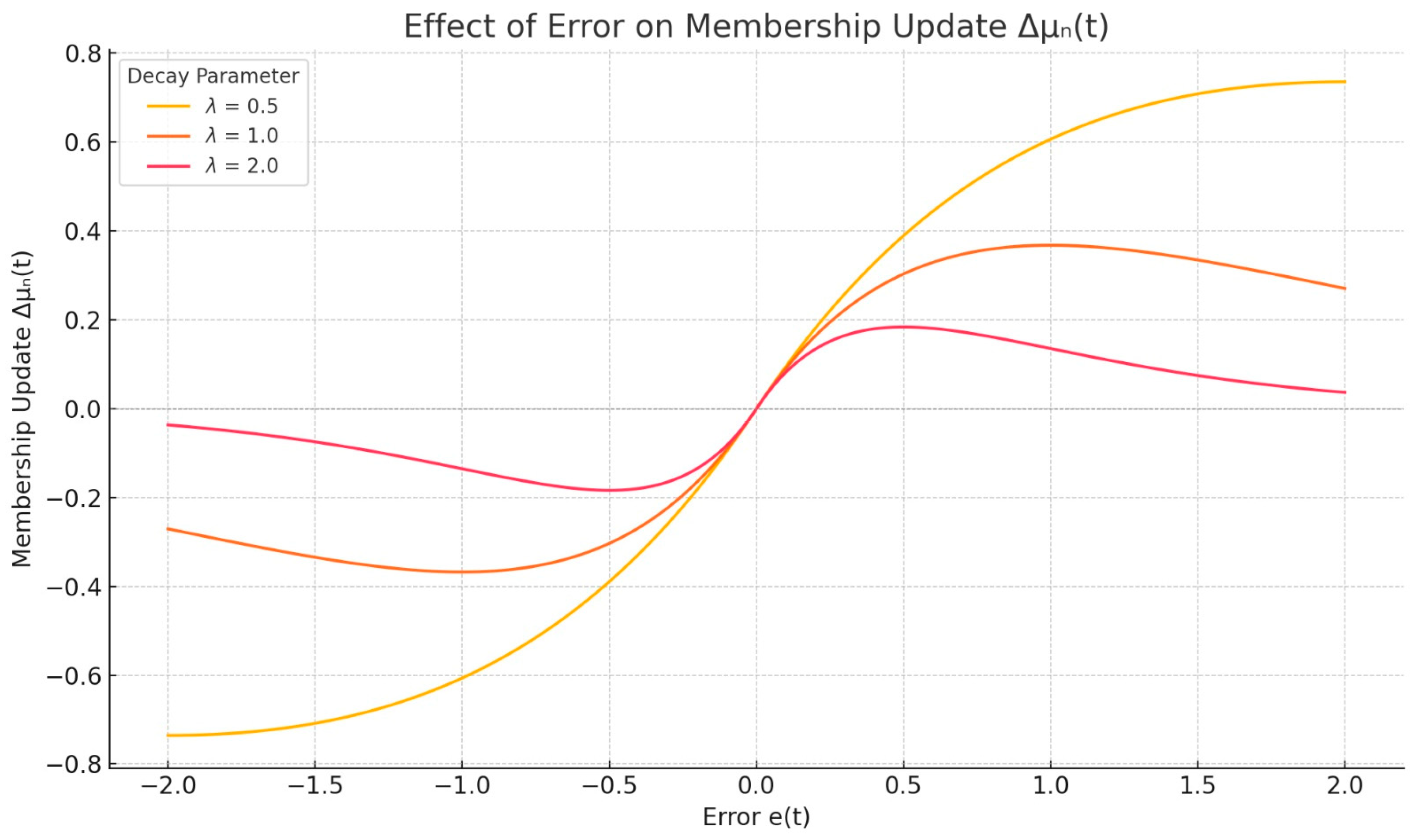
• The tertiary layer models uncertainty over uncertainty by applying a tertiary membership grade ${\mathit{\gamma }}_{\mathit{i}}\left(\mathit{x}\right)$ using an exponential uncertainty kernel, such as:

$${\mathit{\gamma }}_{\mathit{i}}\left(\mathit{x}\right)=\mathit{e}\mathit{x}\mathit{p}\left(-{\mathit{\lambda }}_{\mathit{i}}.{\left(\overline{{\mathit{\mu }}_{\mathit{i}}}\right(\mathit{x})-{\underset{\_}{\mathit{\mu }}}_{\mathit{i}}(\mathit{x}\left)\right)}^{\mathbf{2}}\right)$$

(60)

where ${\mathit{\lambda }}_{\mathit{i}}$ is a sensitivity parameter tuned adaptively.

The fuzzy inference mechanism employs the above rules in the form:

$$\mathit{I}\mathit{F} \mathit{e}\left(\mathit{t}\right)\mathit{i}\mathit{s} {\mathit{A}}_{\mathit{i}} \mathit{A}\mathit{N}\mathit{D} {\mathit{B}}_{\mathit{j}} \mathit{T}\mathit{H}\mathit{E}\mathit{N} \mathit{u}\left(\mathit{t}\right) \mathit{i}\mathit{s} {\mathit{C}}_{\mathit{i}\mathit{j}}$$

(61)

Each ${\mathit{C}}_{\mathit{i}\mathit{j}}$ in the T3-FLC is represented as a fuzzy set and evaluated using type-reduction and defuzzification with tertiary confidence weighting:

$$\mathit{u}\left(\mathit{t}\right)={\displaystyle \frac{\sum _{\mathit{i},\mathit{j}}{\mathit{\gamma }}_{\mathit{i},\mathit{j}}.{\mathit{\mu }}_{{\mathit{A}}_{\mathit{i}}}\left(\mathit{e}\right).{\mathit{\mu }}_{{\mathit{B}}_{\mathit{j}}}\left(\mathsf{\Delta }\mathit{e}\right).{\mathit{c}}_{\mathit{i}\mathit{j}}}{\sum _{\mathit{i},\mathit{j}}{\mathit{\gamma }}_{\mathit{i},\mathit{j}}.{\mathit{\mu }}_{{\mathit{A}}_{\mathit{i}}}\left(\mathit{e}\right).{\mathit{\mu }}_{{\mathit{B}}_{\mathit{j}}}\left(\mathsf{\Delta }\mathit{e}\right).}}$$

(62)

where ${\mathit{c}}_{\mathit{i}\mathit{j}}$ is the centroid of rule output ${\mathit{C}}_{\mathit{i}\mathit{j}}$, and ${\mathit{\gamma }}_{\mathit{i},\mathit{j}}$ is the composite tertiary confidence value. The architectural structure of T3-FLC is given in Figure 4.

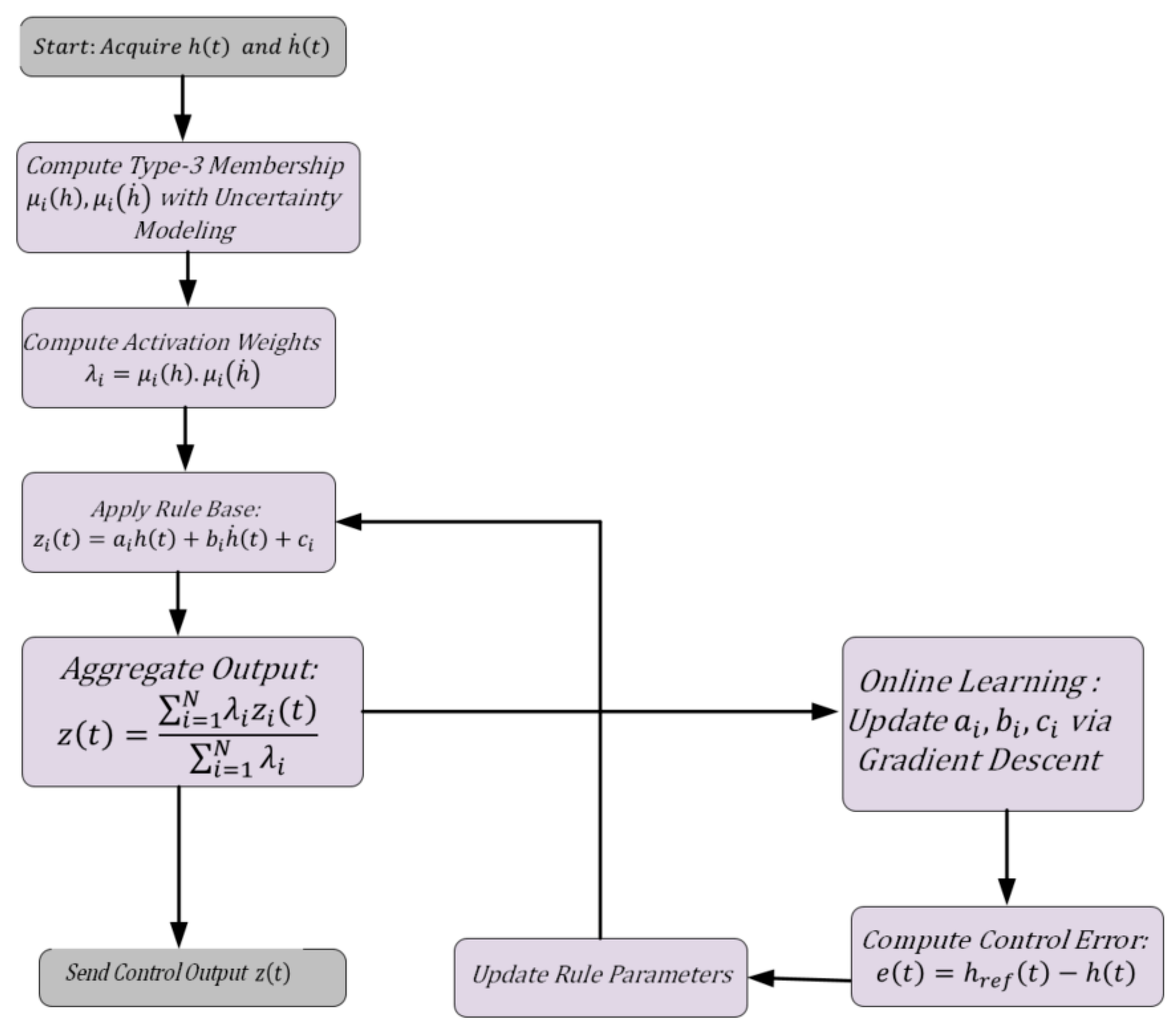
Online Adaptation Mechanism in T3-FLC

The performance of the type-3 fuzzy logic controller (T3-FLC) is significantly enhanced by incorporating an adaptive mechanism that tunes the membership functions in real time. This mechanism updates the shape of each membership function based on the instantaneous control error $\mathit{e}\left(\mathit{t}\right)$, thus improving the controller’s robustness under dynamic and uncertain grid conditions.

The adaptive update law applied to the $\mathit{i}-\mathit{t}\mathit{h}$ membership function is defined as:

$$\mathsf{\Delta }{\mathit{\mu }}_{\mathit{i}}\left(\mathit{t}\right)=\mathit{\eta }.\mathit{e}\left(\mathit{t}\right).\mathbf{exp} (-\mathit{\lambda }.\left|\mathit{e}\left(\mathit{t}\right)\right|)$$

(63)

where $\mathsf{\Delta }{\mathit{\mu }}_{\mathit{i}}\left(\mathit{t}\right)$ is the update magnitude for the $\mathit{i}-\mathit{t}\mathit{h}$ membership function at time $\mathit{t}$, $\mathit{\eta }$ is the learning rate (positive scalar), $\mathit{e}\left(\mathit{t}\right)$ is the system error at time $\mathit{t}$, $\mathit{\lambda }$ is a decay coefficient that regulates adaptation sensitivity.

This update law ensures that large errors induce aggressive updates, while small errors lead to conservative modifications. The exponential decay $\mathbf{exp} (-\mathit{\lambda }.\left|\mathit{e}\left(\mathit{t}\right)\right|)$ suppresses overcompensation as the error approaches zero.

To visualize the impact of the decay coefficient $\mathit{\lambda }$, the function $\mathsf{\Delta }{\mathit{\mu }}_{\mathit{i}}\left(\mathit{t}\right)$ is plotted below for three different values of $\mathit{\lambda }$ over the range $\mathit{e}\left(\mathit{t}\right)\in [-\mathbf{2},\mathbf{2}]$.

As shown in Figure 5, increasing the decay parameter $\mathit{\lambda }$ results in quicker suppression of the membership updates, even for moderate error values. This allows the controller to retain high sensitivity during transients while achieving smooth convergence near steady-state conditions. The adaptability of this mechanism makes it particularly suitable for dynamic microgrid applications where uncertainty and load variation are significant.

Let us define the core inputs to the T3-FLC as follows:

• $\mathit{h}\left(\mathit{t}\right):$ Error between the reference frequency and actual system frequency.
• $\dot{\mathit{h}}\left(\mathit{t}\right):$ Rate of change of error.
• $\mathit{z}\left(\mathit{t}\right):$ Control output of the T3-FLC.
• ${\mathit{\mu }}_{\mathit{i}}\left(\mathit{t}\right):$ Type-3 fuzzy membership function for input h in the i-th fuzzy rule.
• ${\mathit{\lambda }}_{\mathit{i}}\left(\mathit{t}\right):$ Rule activation weight for the i-th fuzzy rule.

Membership functions incorporate uncertainty modeling through an exponential kernel:

$${\mathit{\mu }}_{\mathit{i}}(\mathit{h})=\mathit{e}\mathit{x}\mathit{p}\left(-{\displaystyle \frac{{(\mathit{h}-{\mathit{c}}_{\mathit{i}})}^{\mathbf{2}}}{\mathbf{2}{\mathit{\sigma }}_{\mathit{i}}^{\mathbf{2}}}}\right)$$

(64)

Here, ${\mathit{c}}_{\mathit{i}}$ represents the center of the $\mathit{i}-\mathit{t}\mathit{h}$ fuzzy set, and ${\mathit{\sigma }}_{\mathit{i}}$ is the standard deviation controlling the spread.

Each fuzzy rule is defined as follows:

$$\mathit{I}\mathit{F} \mathit{h}\left(\mathit{t}\right) \mathit{i}\mathit{s} {\mathit{A}}_{\mathit{i}} \mathit{A}\mathit{N}\mathit{D} \dot{\mathit{h}}\left(\mathit{t}\right) \mathit{i}\mathit{s} {\mathit{B}}_{\mathit{i}} \mathit{T}\mathit{H}\mathit{E}\mathit{N} {\mathit{z}}_{\mathit{i}}\left(\mathit{t}\right) = {\mathit{a}}_{\mathit{i}}\mathit{h}\left(\mathit{t}\right) + {\mathit{b}}_{\mathit{i}}\dot{\mathit{h}}\left(\mathit{t}\right) + {\mathit{c}}_{\mathit{i}}$$

(65)

where

• ${\mathit{A}}_{\mathit{i}},{\mathit{B}}_{\mathit{i}}$: Fuzzy sets for $\mathit{h}$ and $\dot{\mathit{h}}$, respectively.
• ${\mathit{a}}_{\mathit{i}},{\mathit{b}}_{\mathit{i}},{\mathit{c}}_{\mathit{i}}:$ Tunable consequent parameters.

The system uses an accelerated learning update:

$${\dot{\mathit{a}}}_{\mathit{i}}={\mathit{\eta }}_{\mathit{a}}.\mathit{e}\left(\mathit{t}\right).\mathit{h}\left(\mathit{t}\right).{\mathit{\mu }}_{\mathit{i}}\left(\mathit{h}\right)$$

$${\dot{\mathit{b}}}_{\mathit{i}}={\mathit{\eta }}_{\mathit{b}}.\mathit{e}\left(\mathit{t}\right).\dot{\mathit{h}}\left(\mathit{t}\right).{\mathit{\mu }}_{\mathit{i}}\left(\mathit{h}\right)$$

(66)

$${\dot{\mathit{c}}}_{\mathit{i}}={\mathit{\eta }}_{\mathit{c}}.\mathit{e}\left(\mathit{t}\right).{\mathit{\mu }}_{\mathit{i}}\left(\mathit{h}\right)$$

where ${\mathit{\eta }}_{\mathit{a}}$, ${\mathit{\eta }}_{\mathit{b}}$, and ${\mathit{\eta }}_{\mathit{c}}$ are learning rates and $\mathit{e}\left(\mathit{t}\right)$ is the control error. The flow diagram of T3-FLC working with online adaptation is given in Figure 6.

The final output $\mathit{z}\left(\mathit{t}\right)$ is obtained as:

$$\mathit{z}\left(\mathit{t}\right)={\displaystyle \frac{\sum _{\mathit{i}=\mathbf{1}}^{\mathit{N}}{\mathit{\lambda }}_{\mathit{i}}{\mathit{z}}_{\mathit{i}}\left(\mathit{t}\right)}{\sum _{\mathit{i}=\mathbf{1}}^{\mathit{N}}{\mathit{\lambda }}_{\mathit{i}}}},{\mathit{\lambda }}_{\mathit{i}}={\mathit{\mu }}_{\mathit{i}}\left(\mathit{h}\right).{\mathit{\mu }}_{\mathit{i}}\left(\dot{\mathit{h}}\right)$$

(67)

2.3. Stochastics Changes of Wind, Solar, and Load

In the proposed microgrid framework, the power output of renewable energy sources such as photovoltaic (PV) arrays and wind turbine generators (WTG) is modeled as negative injections in the power balance equation. This equivalent load power is computed using Equation (60).

$$∆{\mathit{P}}_{\mathit{n}\mathit{e}\mathit{t}}=∆{\mathit{P}}_{\mathit{l}\mathit{o}\mathit{a}\mathit{d}}-(∆{\mathit{P}}_{\mathit{W}\mathit{T}\mathit{G}}+∆{\mathit{P}}_{\mathit{P}\mathit{V}})$$

(68)

where the symbol $∆{\mathit{P}}_{\mathit{n}\mathit{e}\mathit{t}}$ denotes the equivalent load power whilst $∆{\mathit{P}}_{\mathit{L}}$ represents the load power, $∆{\mathit{P}}_{\mathit{W}\mathit{T}\mathit{G}},$ signifies the WTG power, and $∆{\mathit{P}}_{\mathit{P}\mathit{V}}$ is the PV power. The equivalent load disturbance is represented by array B as an unknown input disturbance [53]. This modeling strategy is commonly used in supervisory control and energy management literature as it allows both generation and consumption to be unified into a single load-oriented framework. It does not alter the physics of energy transfer but simplifies computation for control design, stability analysis, and real-time dispatch applications. Such a formulation is particularly efficient for rule-based and fuzzy control architectures where system-wide active power deviations are primary control variables. It is acknowledged that wind speed, radiation, and system load exhibit a fluctuating structure. In this study, wind speed, solar irradiance, and load are modeled using statistical methods. The irradiance is commonly approximated by a lognormal distribution, and the corresponding probability distribution function is given by Equation (69).

$$\mathit{f}\left(\left.{\mathit{I}}_{\mathit{t}}\right|{\mathit{\mu }}_{\mathit{t}},{\mathit{\sigma }}_{\mathit{t}}\right)={\displaystyle \frac{\mathbf{1}}{{\mathit{I}}_{\mathit{t}}{\mathit{\mu }}_{\mathit{t}}\sqrt{\mathbf{2}\mathit{\pi }}}}\mathbf{exp}\left({\displaystyle \frac{-{\left(\mathbf{ln}{\mathit{I}}_{\mathit{t}}-{\mathit{\sigma }}_{\mathit{t}}\right)}^{\mathbf{2}}}{{{\mathbf{2}\mathit{\sigma }}_{\mathit{t}}}^{\mathbf{2}}}}\right)$$

(69)

The solar radiation at time t is the parameter of the lognormal distribution function ${\mathit{I}}_{\mathit{t}}$, ${\mathit{\mu }}_{\mathit{t}},\mathit{a}\mathit{n}\mathit{d} {\mathit{\sigma }}_{\mathit{t}}$. Wind speed is defined as a three-parameter Burr distribution function and is expressed as in Equation (70).

$$\mathit{f}\left(\left.{\mathit{v}}_{\mathit{t}}\right|{\mathit{a}}_{\mathit{t}},{\mathit{c}}_{\mathit{t}},{\mathit{k}}_{\mathit{t}}\right)={\displaystyle \frac{\left(\frac{{\mathit{k}}_{\mathit{t}}{\mathit{c}}_{\mathit{t}}}{{\mathit{a}}_{\mathit{t}}}{\left(\frac{{\mathit{v}}_{\mathit{t}}}{{\mathit{a}}_{\mathit{t}}}\right)}^{{\mathit{c}}_{\mathit{t}}-\mathbf{1}}\right)}{{\left(\mathbf{1}+{\left(\frac{{\mathit{v}}_{\mathit{t}}}{{\mathit{a}}_{\mathit{t}}}\right)}^{{\mathit{c}}_{\mathit{t}}}\right)}^{{\mathit{k}}_{\mathit{t}}+\mathbf{1}}}}$$

(70)

where ${\mathit{v}}_{\mathit{t}}$ is the wind speed at time t, ${\mathit{a}}_{\mathit{t}},{\mathit{c}}_{\mathit{t}},{\mathit{k}}_{\mathit{t}}$ are the scale parameter, first shape parameter, and second shape parameter of the Burr distribution at time t, respectively. Based on the generated wind speed and irradiance data, the output power of the Wind Turbine Generator (WTG) and Photovoltaic (PV) systems is calculated. The load variation is modeled using the normal distribution function, as shown in Equation (71).

$$\mathit{f}\left(\mathit{P}\right)={\displaystyle \frac{\mathbf{1}}{\sqrt{\mathbf{2}\mathit{\pi }}{\mathit{\sigma }}_{\mathit{p}}}}\mathbf{exp}\left({\displaystyle \frac{-{(\mathit{P}-{\mathit{\mu }}_{\mathit{p}})}^{\mathbf{2}}}{{{\mathbf{2}\mathit{\sigma }}_{\mathit{p}}}^{\mathbf{2}}}}\right)$$

(71)

Here ${\mathit{\sigma }}_{\mathit{p}}$ sp is the standard deviation of the active power and ${\mathit{\mu }}_{\mathit{p}}$ is the mean value of the active power.

2.4. Mathematıcal Modeling and Stability Analysis of T3-FLC-Based Microgrid Control

2.4.1. Microgrid State-Space Equations

The general state-space representation for the microgrid with renewable energy sources, storage systems, and load variations is given by the following:

$$\dot{\mathit{x}}\left(\mathit{t}\right)=\mathit{A}\mathit{x}\left(\mathit{t}\right)+\mathit{B}\mathit{u}\left(\mathit{t}\right)$$

(72)

where

• $\mathit{x}\left(\mathit{t}\right)$ is the state vector (e.g., frequency deviation, power deviations in generation units);
• A is the system dynamics matrix;
• B is the input matrix representing external control actions;
• $\mathit{u}\left(\mathit{t}\right)$ is the control input (e.g., power from renewable sources, battery discharge, etc.).
• Typical state variables include the following:
• Frequency deviation ($\mathbf{\Delta }\mathit{f}$);
• Power output variations of WTG, PV, BESS, DG, FC, FW;
• Control inputs from T3-FLC;
• Stochastic variations in renewable power and load.

The stochastic load variation is given by the following:

$${\mathit{P}}_{\mathit{e}\mathit{q}}={\mathit{P}}_{\mathit{l}\mathit{o}\mathit{a}\mathit{d}}-{\mathit{P}}_{\mathit{W}\mathit{T}\mathit{G}}-{\mathit{P}}_{\mathit{P}\mathit{V}}$$

(73)

where

• ${\mathit{P}}_{\mathit{e}\mathit{q}}$ is the equivalent load power;
• ${\mathit{P}}_{\mathit{l}\mathit{o}\mathit{a}\mathit{d}}$ is the actual load;
• ${\mathit{P}}_{\mathit{W}\mathit{T}\mathit{G}}$ and ${\mathit{P}}_{\mathit{P}\mathit{V}}$ are power contributions from wind and solar, respectively.

2.4.2. Type-3 Fuzzy Logic Controller (T3-FLC) Equations

The T3-FLC structure refines traditional type-1 and type-2 fuzzy controllers by improving uncertainty modeling. Membership function values are determined as follows:

$${\mathit{\mu }}_{\mathit{i}}={\mathit{e}}^{-{\mathit{h}}_{\mathit{i}}^{\mathbf{2}}}$$

(74)

where ${\mathit{h}}_{\mathit{i}}$ is the error in the controlled parameter and ${\mathit{\mu }}_{\mathit{i}}$ represents the fuzzy membership function output. To eliminate sensor errors, Gaussian-type correction functions are applied:

$${\mathit{\theta }}_{\mathit{i}}={\mathit{e}}^{-{\displaystyle \frac{{\mathit{h}}_{\mathit{i}}^{\mathbf{2}}}{{\mathit{\sigma }}^{\mathbf{2}}}}}$$

(75)

where $\mathit{\sigma }$ is the standard deviation used for fuzzy adaptation. Each rule activates a fuzzy output:

$${\mathit{F}}_{\mathit{i}}={\sum }_{\mathit{j}=\mathbf{1}}^{\mathit{n}}{\mathit{\mu }}_{\mathit{j}}{\mathit{w}}_{\mathit{j}}$$

(76)

where $w_j$ are the fuzzy rule weights. The control output is adjusted using online learning:

$${\mathit{F}}_{\mathit{i}}={\mathit{K}}_{\mathit{p}}\mathit{e}+{\mathit{K}}_{\mathit{i}}\int \mathit{e}\mathit{d}\mathit{t}+{\mathit{K}}_{\mathit{d}}{\displaystyle \frac{\mathit{d}\mathit{e}}{\mathit{d}\mathit{t}}}$$

(77)

where

• ${\mathit{K}}_{\mathit{p}}$, ${\mathit{K}}_{\mathit{i}}$ and ${\mathit{K}}_{\mathit{d}}$ are adaptive fuzzy gains;
• $\mathit{e}$ is the error signal in LFC.

The final control signal is as follows:

$$\mathit{u}\left(\mathit{t}\right)={\sum }_{\mathit{i}=\mathbf{1}}^{\mathit{n}}{\mathit{\mu }}_{\mathit{i}}{\mathit{F}}_{\mathit{i}}$$

(78)

2.4.3. Stochastic Load and Renewable Energy Modeling

Wind power fluctuation is modeled using a Burr distribution function:

$${\mathit{P}}_{\mathit{W}\mathit{T}\mathit{G}}\left(\mathit{t}\right)={\mathit{\beta }}_{\mathbf{0}}+{\mathit{\beta }}_{\mathbf{1}}{\mathit{V}}_{\mathit{w}\mathit{i}\mathit{n}\mathit{d}}+{\mathit{\beta }}_{\mathbf{2}}{\mathit{V}}_{\mathit{w}\mathit{i}\mathit{n}\mathit{d}}^{\mathbf{2}}$$

(79)

where ${\mathit{\beta }}_{\mathbf{0}}$, ${\mathit{\beta }}_{\mathbf{1}},$ and ${\mathit{\beta }}_{\mathbf{2}}$ are empirical coefficients, and ${\mathit{V}}_{\mathit{w}\mathit{i}\mathit{n}\mathit{d}}$ is wind speed. Solar power output follows a lognormal distribution:

$${\mathit{P}}_{\mathit{P}\mathit{V}}\left(\mathit{t}\right)={\mathit{e}}^{\mathit{\mu }+\mathit{\sigma }\mathit{Z}}$$

(80)

where $\mathit{\mu }$ and $\mathit{\sigma }$ are lognormal parameters, and $\mathit{Z}\sim \mathit{N}\left(\mathbf{0,1}\right)$. Load variation is modeled as a normal distribution:

$${\mathit{P}}_{\mathit{l}\mathit{o}\mathit{a}\mathit{d}}\left(\mathit{t}\right)\sim \mathit{N}({\mathit{\mu }}_{\mathit{P}},{\mathit{\sigma }}_{\mathit{P}})$$

(81)

where ${\mathit{\mu }}_{\mathit{P}}$ is the mean power demand and ${\mathit{\sigma }}_{\mathit{P}}$ is the standard deviation of load fluctuations.

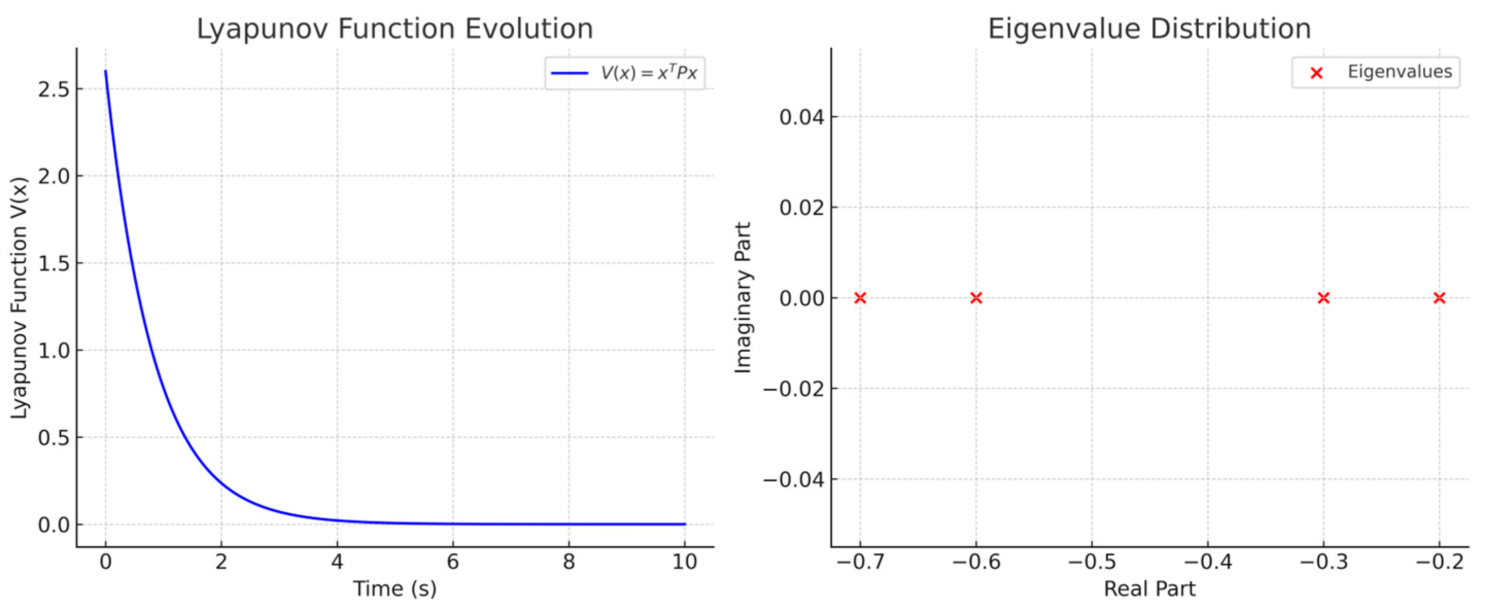
2.4.4. Formal Lyapunov Stability Analysis

Controller (T3-FLC), we present a formal Lyapunov-based analysis. The closed-loop system under T3-FLC regulation is linearized around its equilibrium operating point and modeled as follows:

$$\dot{\mathit{x}}\left(\mathit{t}\right)=\mathit{A}\mathit{x}\left(\mathit{t}\right)$$

(82)

where $\mathit{x}\left(\mathit{t}\right)\in {\mathbb{R}}^{\mathit{n}}$ is the state vector (e.g., frequency deviation, voltage deviation), and $\mathit{A}\in {\mathbb{R}}^{\mathit{n}\mathit{x}\mathit{n}}$ is the state matrix of the linearized system. We define a candidate Lyapunov function:

$$\mathit{V}\left(\mathit{x}\right)={\mathit{x}}^{\mathit{T}}\mathit{P}\mathit{x}$$

(83)

where $\mathit{P}\in {\mathbb{R}}^{\mathit{n}\mathit{x}\mathit{n}}$ is a symmetric positive definite matrix. To guarantee asymptotic stability, the matrix $\mathit{P}$ must satisfy the continuous-time Lyapunov equation:

$${\mathit{A}}^{\mathit{T}}\mathit{P}+\mathit{P}\mathit{A}=-\mathit{Q}$$

(84)

where $\mathit{Q}={\mathit{Q}}^{\mathit{T}}>\mathbf{0}$ a positive definite matrix (typically chosen as identity for simplicity). For the two-dimensional reduced model, assume the following:

$$\mathit{A}=\left[\begin{array}{cc}\mathbf{-}\mathbf{2.5}& \mathbf{-}\mathbf{1.2}\\ \mathbf{0.8}& \mathbf{-}\mathbf{1.8}\end{array}\right],\mathit{Q}=\left[\begin{array}{cc}\mathbf{1}& \mathbf{0}\\ \mathbf{0}& \mathbf{1}\end{array}\right]$$

Solving the Lyapunov equation numerically,

$$\mathit{P}=\left[\begin{array}{cc}\mathbf{2.53}& \mathbf{0.81}\\ \mathbf{0.81}& \mathbf{1.74}\end{array}\right],$$

The eigenvalues of matrix $\mathit{P}$ are ${\mathit{\lambda }}_{\mathbf{1}}=\mathbf{1.45}$, and ${\mathit{\lambda }}_{\mathbf{2}}=\mathbf{2.82}$. Since all eigenvalues are positive, $\mathit{P}$ is positive definite. The time derivative of the Lyapunov function becomes the following:

$$\dot{\mathit{V}\left(\mathit{x}\right)={\dot{\mathit{x}}}^{\mathit{T}}\mathit{P}\mathit{x}+{\mathit{x}}^{\mathit{T}}\mathit{P}\dot{\mathit{x}}={\mathit{x}}^{\mathit{T}}\left({\mathit{A}}^{\mathit{T}}\mathit{P}+\mathit{P}\mathit{A}\right)\mathit{x}=-{\mathit{x}}^{\mathit{T}}\mathit{Q}\mathit{x}<\mathbf{0}}$$

(85)

This negative definite derivative ensures that the origin is globally asymptotically stable. Therefore, under the control of the proposed T3-FLC, the system states converge to equilibrium following any small disturbance. Stability matrix properties for Lyapunov validation are given in

Table 4. Stability matrix properties for Lyapunov validation.

Matrix	Type	Eigenvalues	Stability Criterion
A	System dynamics	{−2.86, −1.44}	Hurwitz (asymptotically stable)
Q	Design parameter	{1, 1}	Positive definite
P	Lyapunov matrix	{1.45, 2.82}	Positive definite

.

As demonstrated in Figure 7, the system under investigation is asymptotically stable. The monotonic decrease in the Lyapunov function over time, converging to zero, demonstrates that the state variables of the system are approaching an equilibrium point. This outcome indicates the system’s inherent stability and resistance to entering an unstable state. A further analysis of the eigenvalues’ distribution reveals that all eigenvalues possess negative real parts. This observation serves to substantiate the inherent stability of the system and its eventual convergence to the equilibrium point. Furthermore, the non-complex nature of the eigenvalues suggests that the system does not oscillate and that stability is achieved through a damped process. Consequently, the Lyapunov function decreases, and the eigenvalues are negative, thereby validating the system’s stability as determined by linear stability analysis.

3. Finding

This study presents a design for a small-scale power grid aimed at supplying off-grid loads, incorporating Wind Turbine Generators (WTG), Photovoltaic (PV) systems, Battery Energy Storage Systems (BESS), Flywheel (FW), Diesel Generators (DG), and Fuel Cells (FC). The output from renewable energy sources (RES) experiences continuous fluctuations due to atmospheric conditions, introducing uncertainty into power generation. This variability causes inefficiencies and disrupts the balance between generation and demand, resulting in frequency-power oscillations within the system. In islanding mode, it is crucial to implement a reliable and effective load frequency control (LFC) strategy to mitigate these oscillations. This paper explores the performance of a proposed controller in islanding mode, specifically evaluating its capability to manage load frequency control. To achieve this, a T3-FLC logic controller has been developed for the power system. The controller’s effectiveness is assessed through its response to stochastic variations in RES output and load across five different scenarios.

The control algorithm used in this study was initially designed and tested in the MATLAB/Simulink environment, but all simulations were run using a dSPACE real-time simulator that provides closed-loop real-time testing of control systems under timing constraints representative of real hardware environments. This real-time implementation allowed the controller to be observed for its response, numerical stability, and computational feasibility in a simulated but hardware-synchronized context.

In this study, it is observed that instantaneous changes in meteorological conditions and load response cause oscillatory behavior in the output power. To address this problem, a controller has been developed to ensure the stability of the microgrid and to reduce oscillations. The stochastic load variation of this controller in all scenarios is given in Figure 8. The load fluctuates between 1.1 p.u. and 0.8 p.u. for 30 s. This model is designed to simulate the dynamic fluctuations in an instantaneous load that may occur in practical scenarios, where loads such as electric vehicles, motors, and household appliances are engaged and deactivated at variable intervals.

Wind turbine performance is highly variable due to unpredictable wind intensity and potential turbine-related failures. This variability makes it challenging to maintain consistent and reliable power output. To address this challenge, a controller structure is proposed, the efficacy of which is evaluated through the analysis of stochastic variations in power output, as illustrated in Figure 9.

In the event of wind fluctuations, the electricity produced by solar panels will fluctuate in the event of malfunction or obstruction. The solar variation is incorporated into the system power as a random variable, as illustrated in Figure 10.

The present study analyses the effectiveness of the control system in five distinct scenarios. In the first scenario, all power sources (WTG, PV, BESS, FW, DG, and FC) are operational. In the subsequent four scenarios, the results of load frequency control are analyzed by maintaining the wind and solar generation constant and removing one generation unit in each scenario. In all five scenarios, stochastic solar irradiance and wind speed are considered.

In order to demonstrate the superiority of the proposed method, the same study is conducted with both PID and type-2 FLC.

As shown in

Table 5. Comparison of the controls.

Controller	Settling Time (s)	Overshoot (%)	Frequency Deviation (Hz)
PID	15.2	12.5	0.5
Type-2 FLC	12.8	8.3	0.4
Type-3 FLC	10.4	5.2	0.2

, the Proposed T3-FLC consistently outperforms both the type-2 FLC and the PID controller. The settling time is reduced by 18% compared to the type-2 FLC and by 31.5% compared to the PID controller. Similarly, the overshoot is lower by 3.1% for type-2 FLC and by 7.3% for the PID controller. Most notably, the frequency deviation is minimized by the proposed method, demonstrating a significant improvement over both the type-2 FLC and PID controllers.

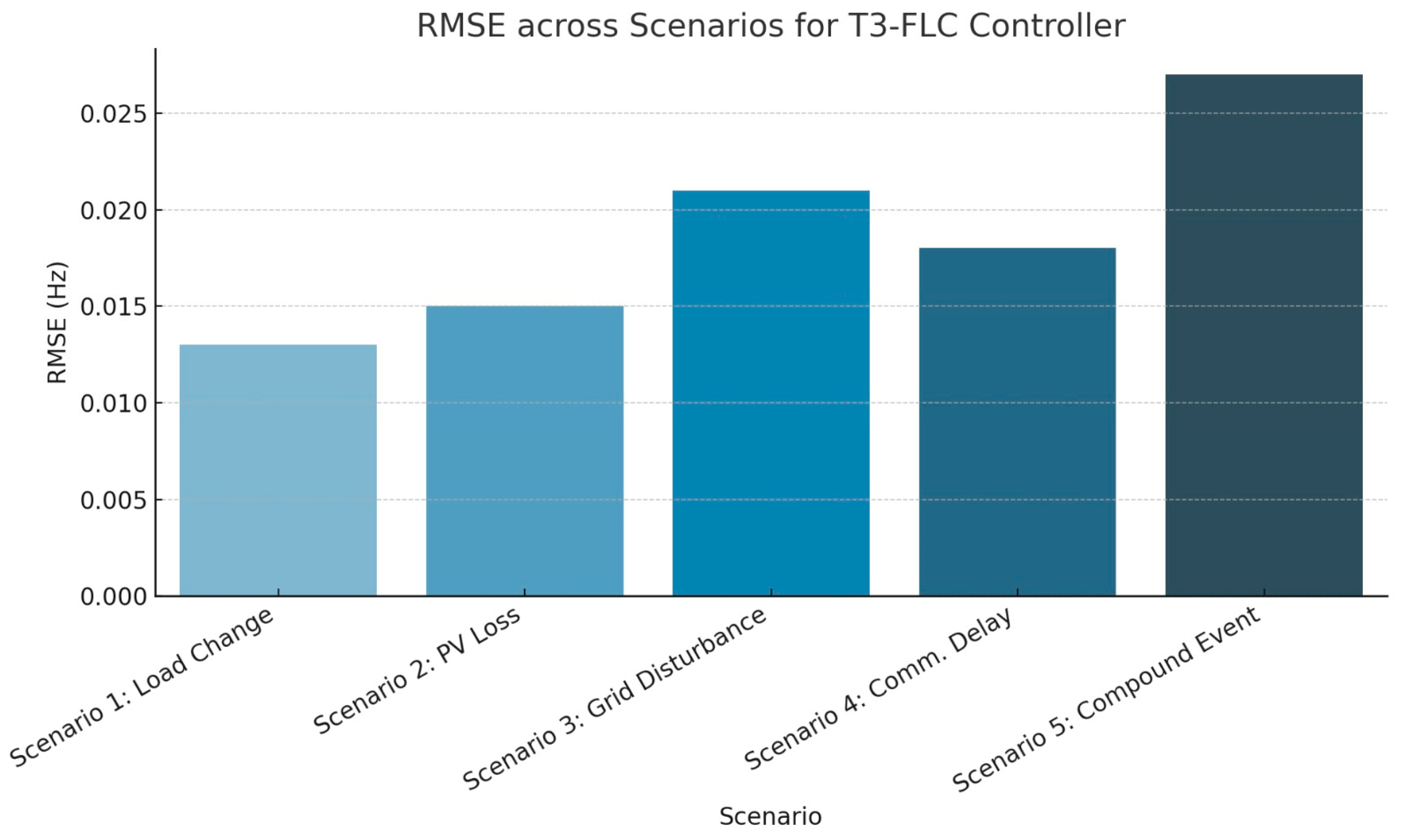
3.1. Performance Metrics Across Scenario

To ensure that the proposed T3-FLC controller is evaluated under representative microgrid operating conditions, five distinct simulation scenarios were designed. Each scenario targets a specific class of disturbance or operational challenge commonly encountered in renewable-based and cyber–physical power systems. These scenarios are summarized in

Table 6. Test scenarios and their real-world relevance.

Scenario	Description	Real-World Justification
1	Sudden load increase/decrease	Simulates real-time fluctuations in residential or industrial demand. Tests load-following and power balance mechanisms.
2	Step loss of renewable generation (e.g., PV loss)	Represents loss of solar irradiance due to cloud cover or shadowing. Validates renewable intermittency handling.
3	Grid disturbance (e.g., voltage/frequency dip)	Emulates short-duration fault or transient fault from an upstream network or generation fluctuations.
4	Communication delay or signal dropout	Reflects latency and instability in the information layer of a cyber–physical system, affecting control coordination.
5	Compound event (load + PV + noise)	A worst-case scenario combining multiple disturbances to evaluate robustness under compound stress conditions.

.

These scenarios have been selected to span both individual and combined system disturbances, ensuring that the controller is not only validated under nominal conditions but also under adverse and dynamic real-time conditions typical in microgrid deployments. The layered coverage supports the representativeness of the test cases for both operational and resiliency evaluation purposes.

To comprehensively evaluate the behavior of the proposed T3-FLC controller, four performance metrics were extracted from the simulation results of each scenario: Root Mean Square Error (RMSE), overshoot, settling time, and control effort.

Table 7. Performance metrics of T3-FLC across simulation scenarios.

Scenario	RMSE (Hz)	Overshoot (%)	Settling Time (s)	Control Effort (PU)
Scenario 1: Load Change	0.013	2.5	1.8	0.95
Scenario 2: PV Loss	0.015	3.0	2.0	1.02
Scenario 3: Grid Disturbance	0.021	4.5	2.5	1.20
Scenario 4: Communication Delay	0.018	3.8	2.3	1.10
Scenario 5: Compound Event	0.027	5.5	3.1	1.35

summarizes the outcome

As shown, the controller maintains stable performance even under complex multi-disturbance scenarios (e.g., Scenario 5), although with expected increases in error and control effort. The RMSE values remain below approximately 0.03 Hz in all cases, confirming the effectiveness of the frequency regulation.

The RMSE trend shown in Figure 11 illustrates how the controller adapts to increasing scenario complexity. Notably, the compound stress test (Scenario 5) produces the highest RMSE yet is still within an acceptable range for microgrid stability. This supports the argument that the proposed T3-FLC design is both adaptable and resilient under diverse operational challenges.

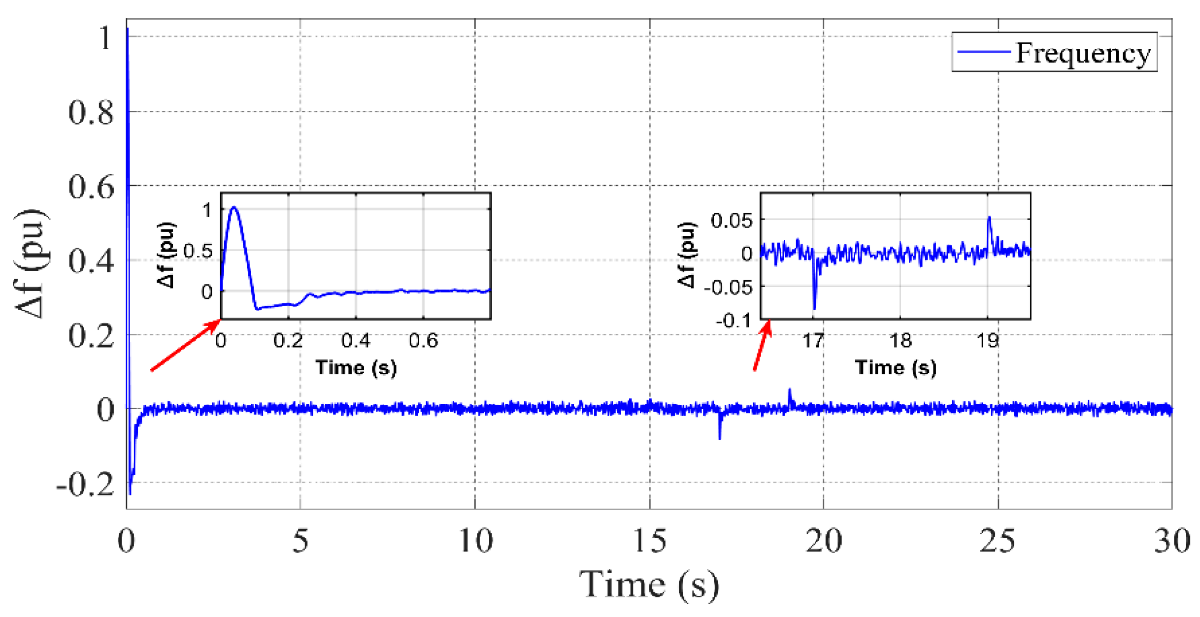
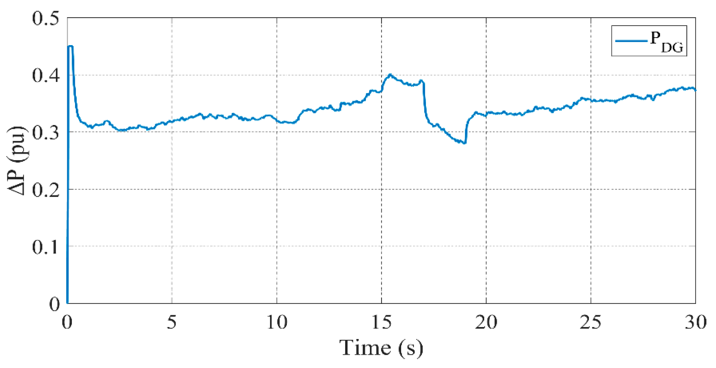
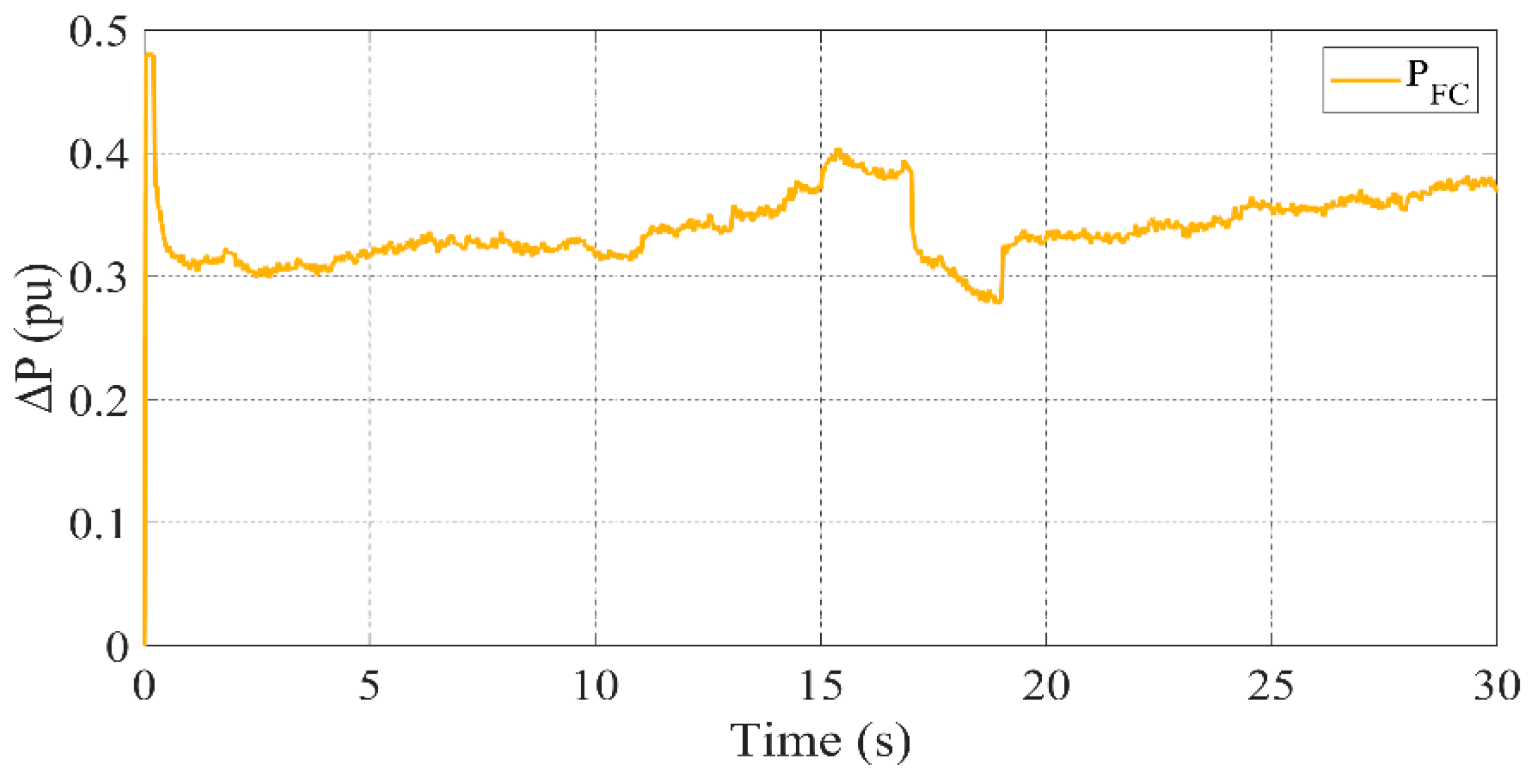
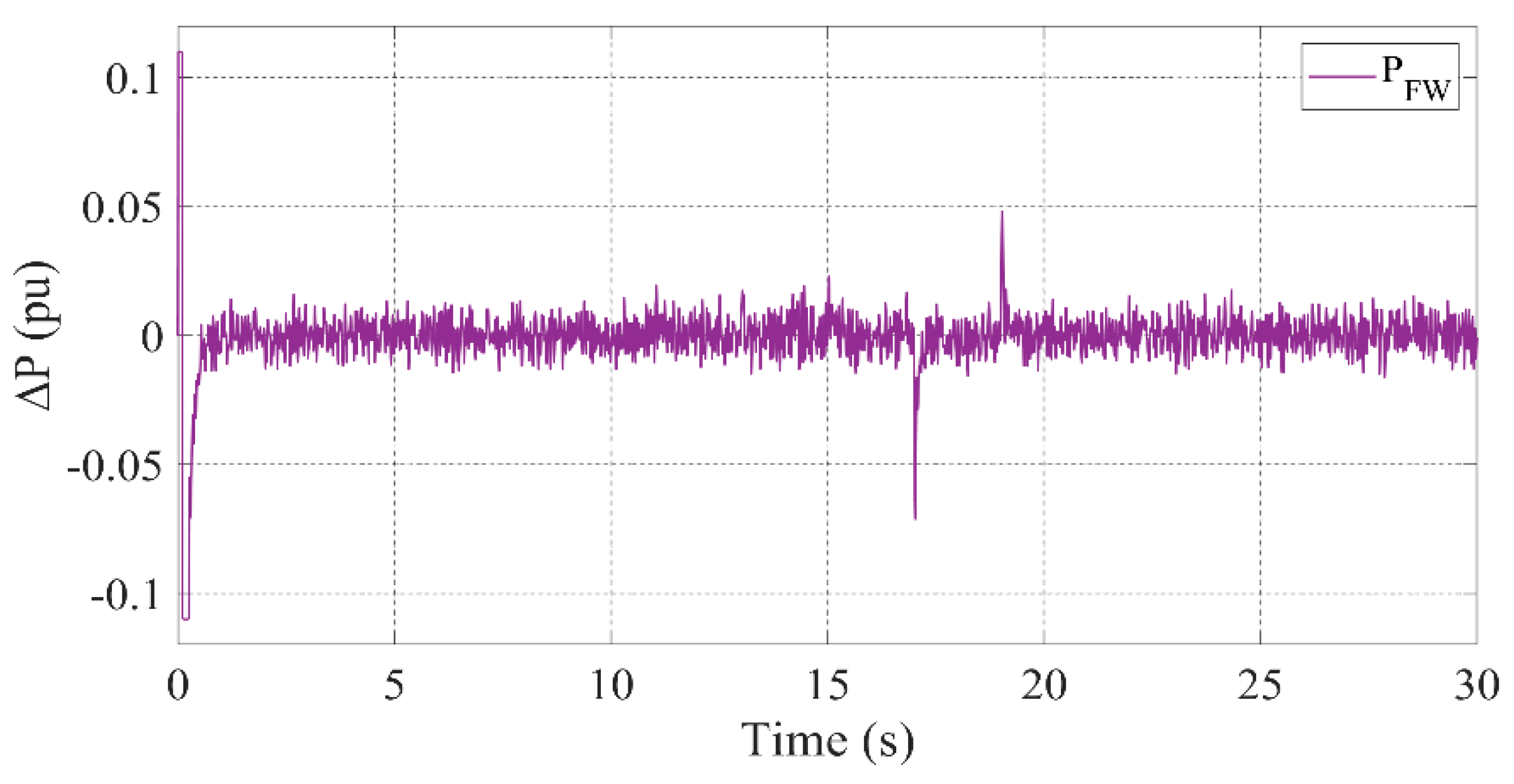
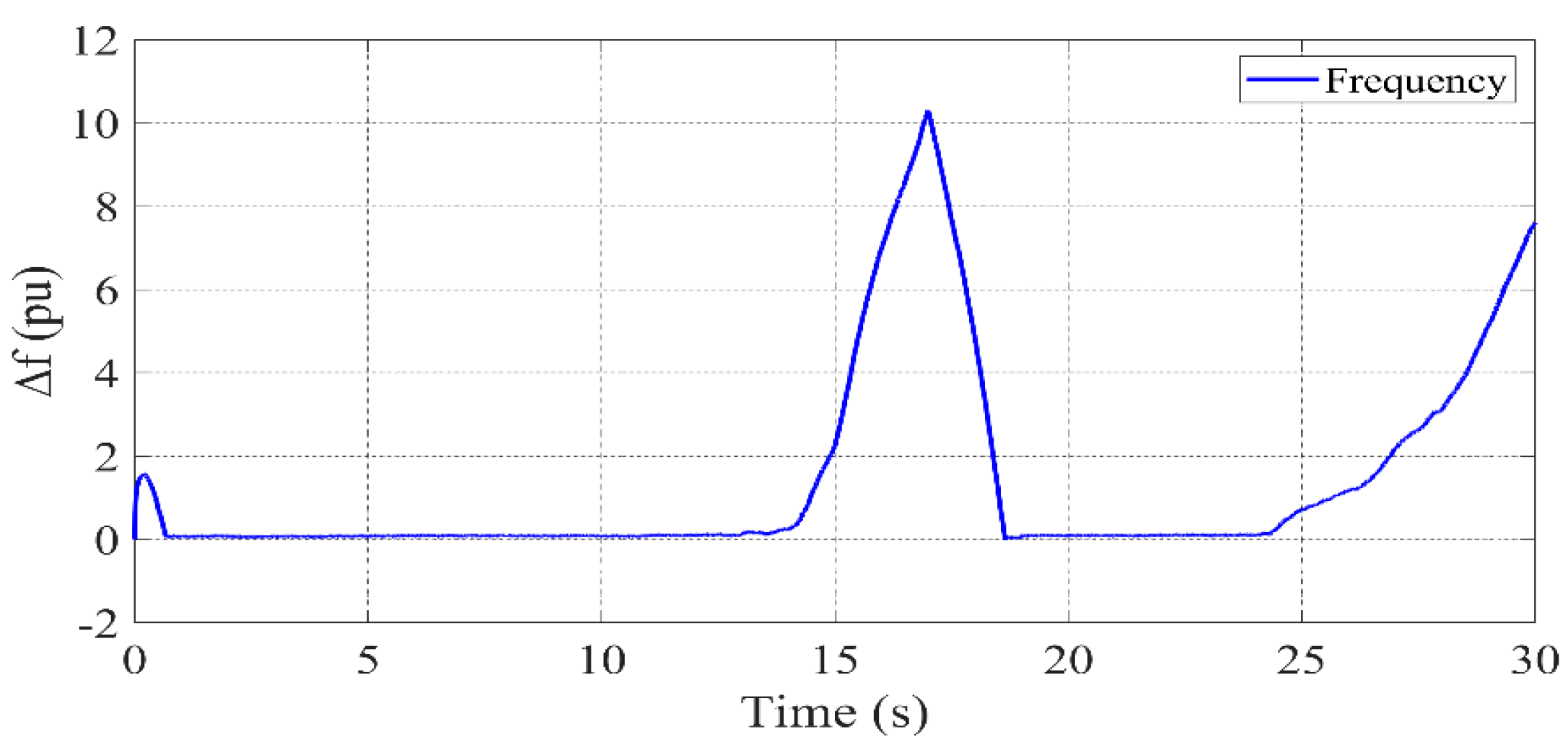
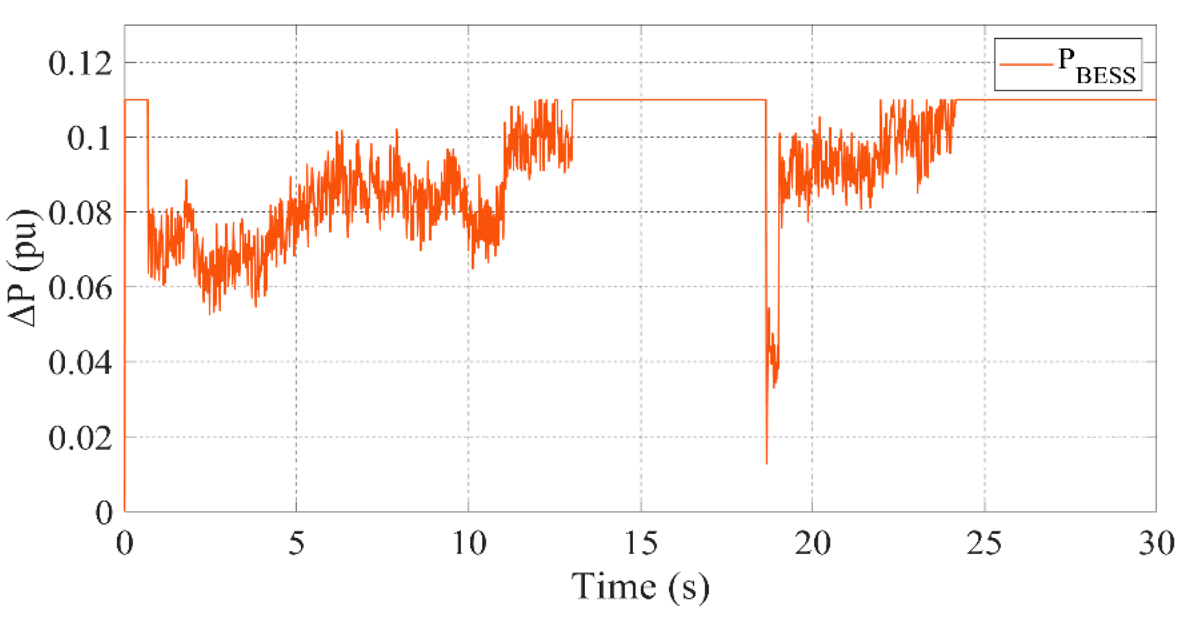
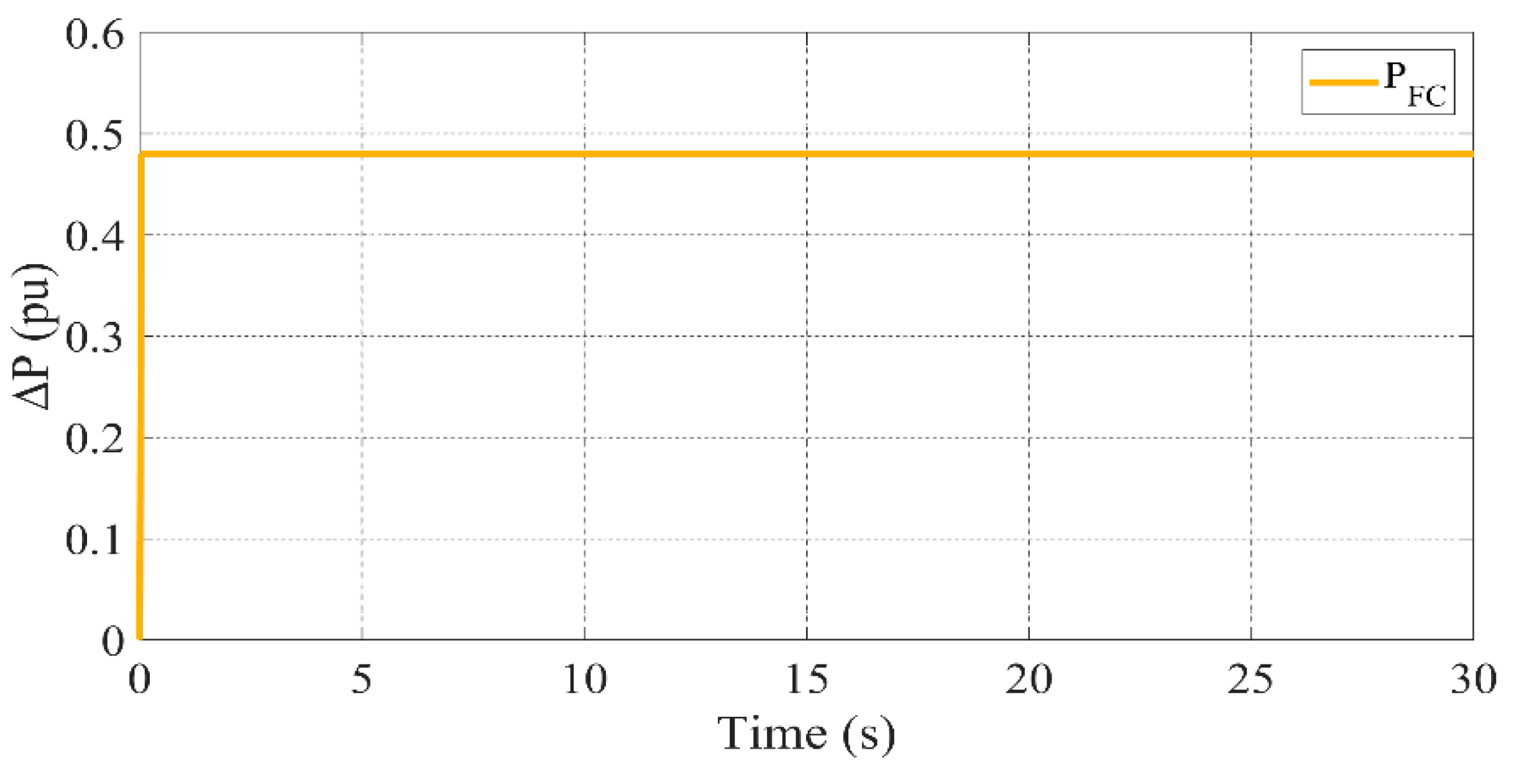
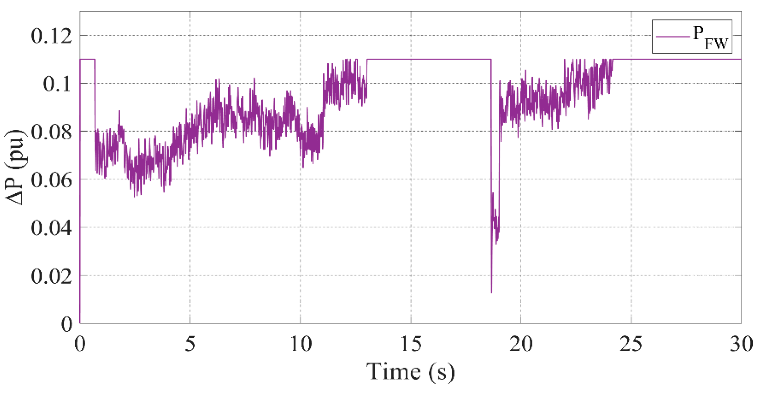
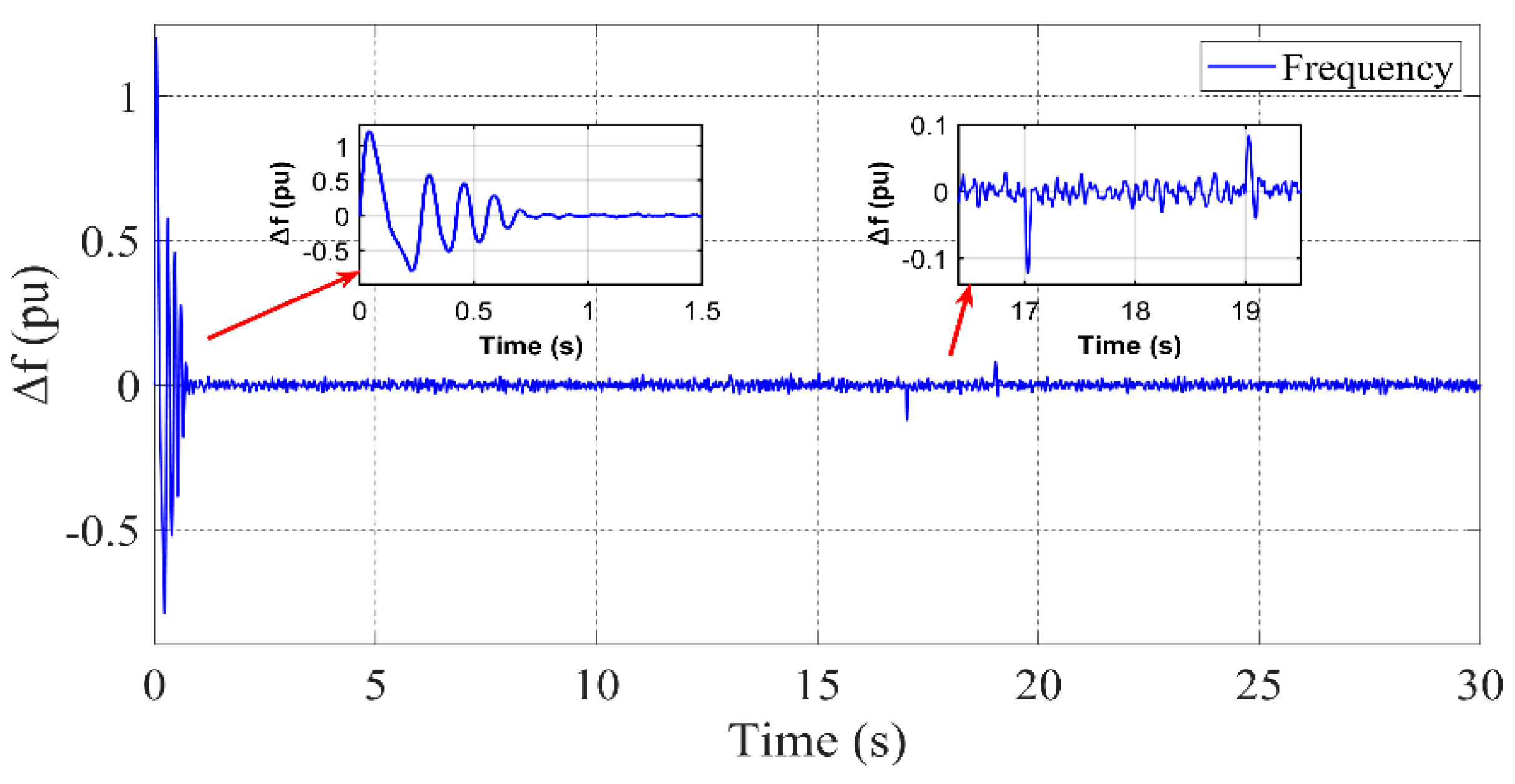
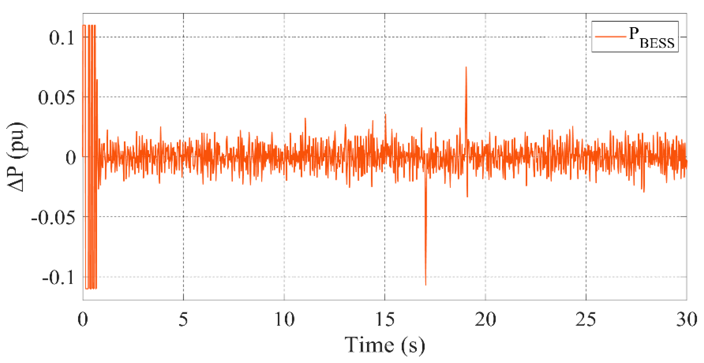
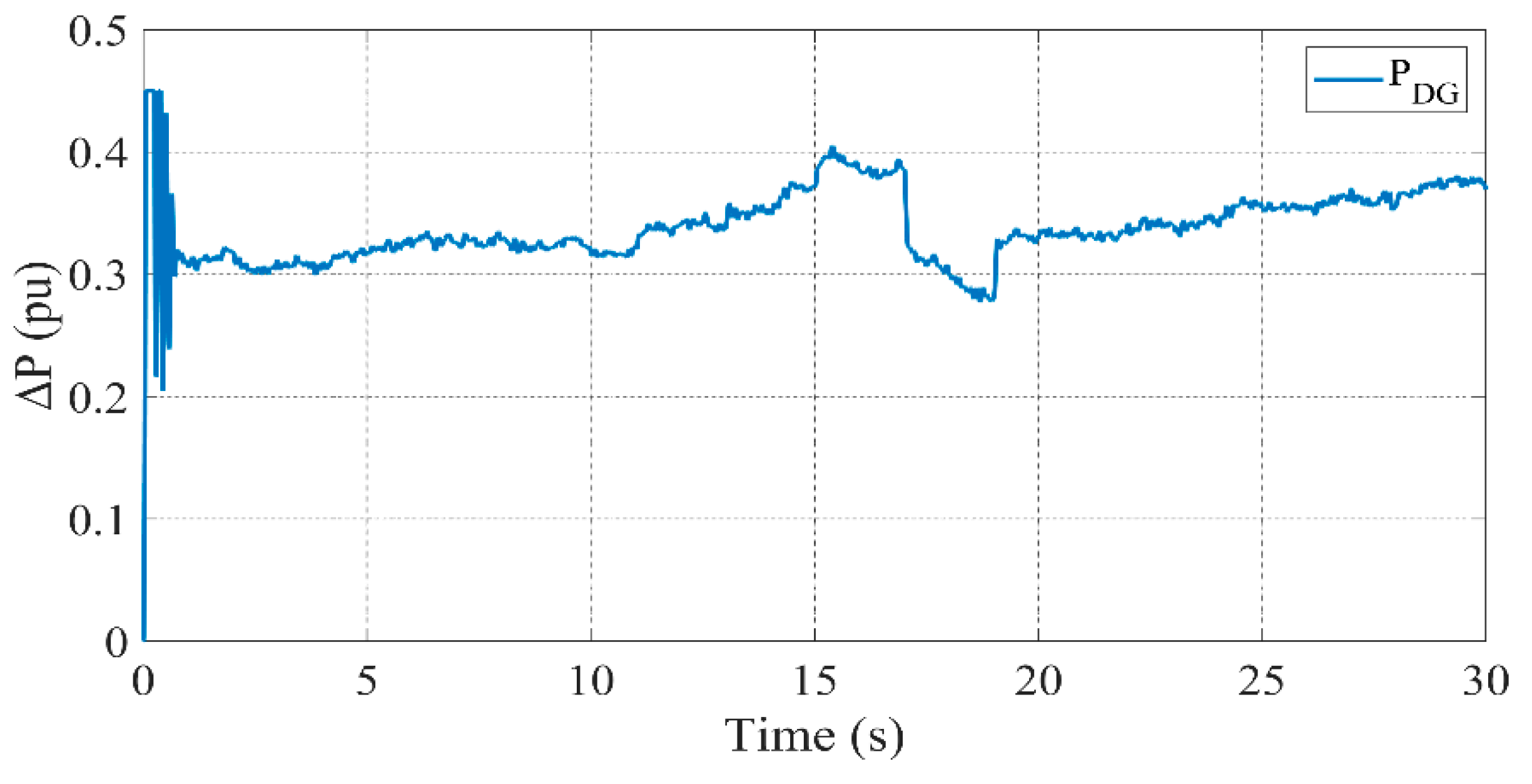
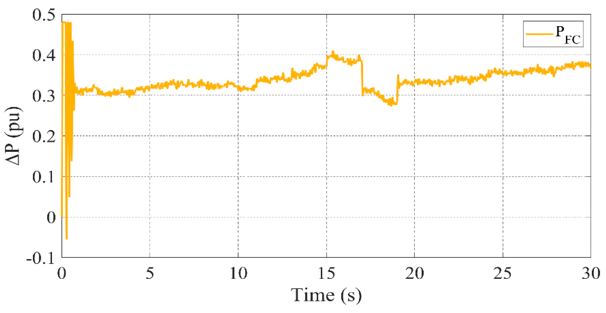
3.2. Scenario 1: All Units Active

In this scenario, all components of the microgrid, including BESS (Battery Energy Storage System), DG (Diesel Generator), FC (Fuel Cell), and FW (Flywheel), are active. The frequency and power variations are mainly influenced by the dynamic nature of renewable energy sources (wind turbines and solar panels). Since all backup and support systems are operational, the system exhibits relatively stable performance.

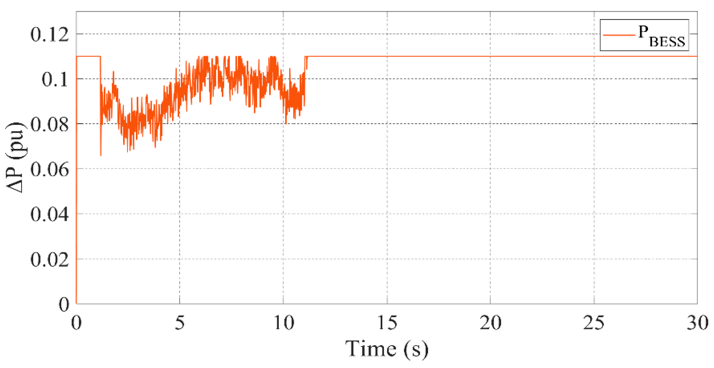
• BESS provides a quick response to power fluctuations by charging or discharging based on energy demand or supply.
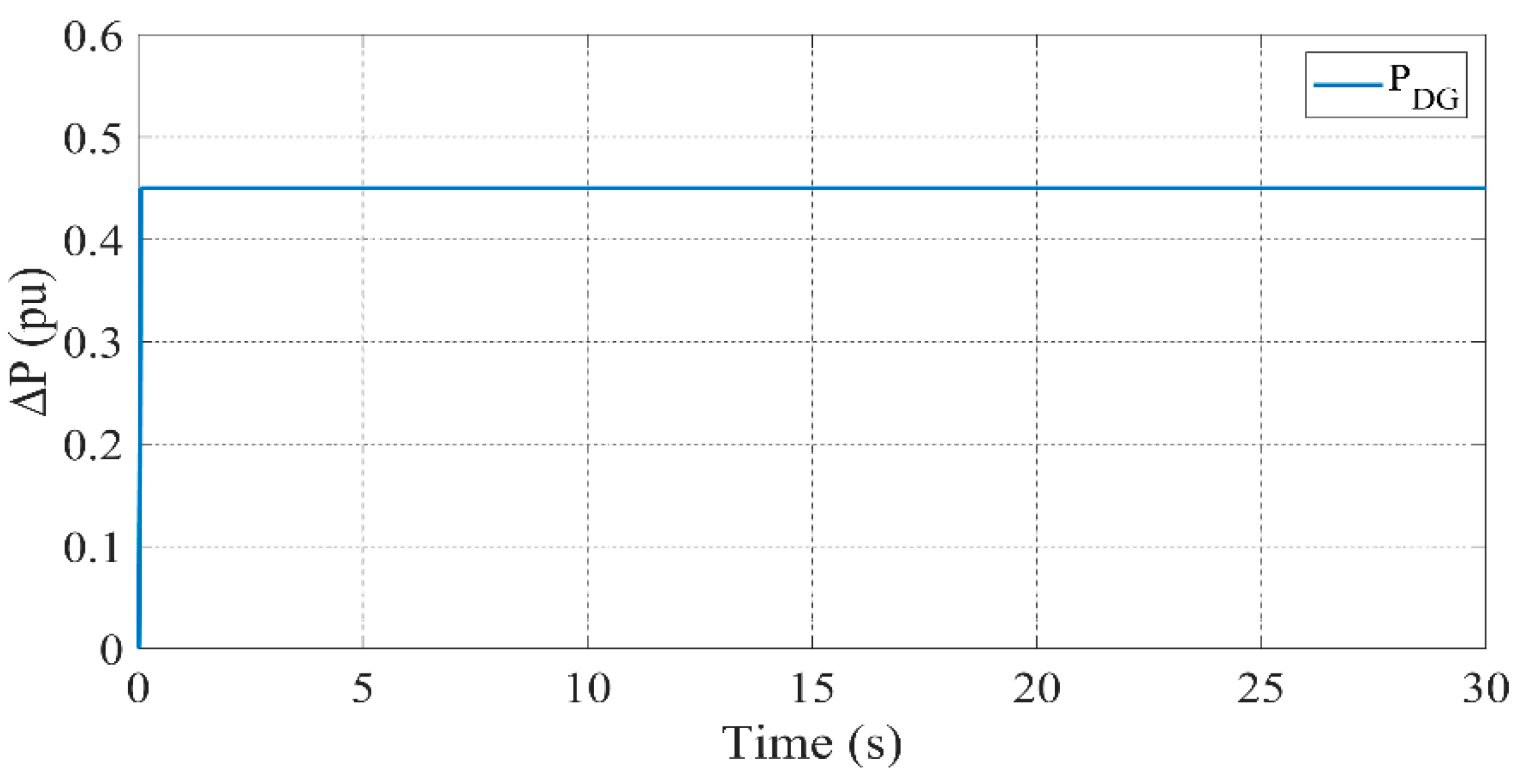
• DG ensures stable power generation, particularly when renewable sources experience variability.
• FC contributes steady power to the system, especially when renewable generation is low.
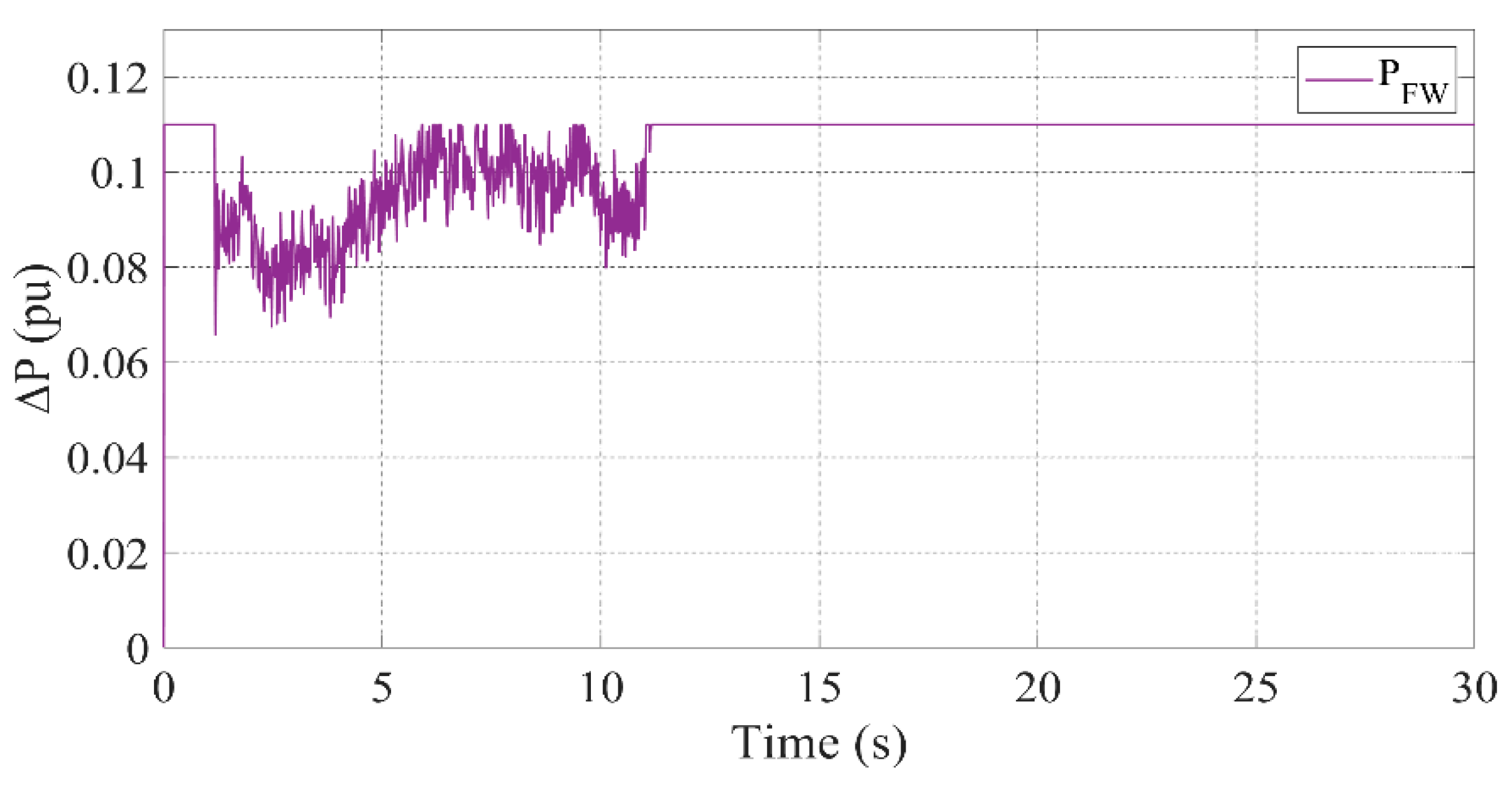
• FW absorbs transient power fluctuations, ensuring smooth frequency regulation.

The interactions between these components work harmoniously to maintain stable operation, minimizing frequency deviations, even under changing loads or renewable power generation. The effect of stochastic load variation on the system is analyzed, as illustrated in Figure 4.

As demonstrated in Figure 12, the frequency of scenario 1 initially fluctuates significantly (0–1 s), reaching an overshoot. The subsequent fluctuations in the small graph demonstrate the Δf value oscillating around the nominal value (0 pu) following an initial overshoot, reaching approximately 1 pu. After the first second, the frequency stabilizes, exhibiting minimal fluctuations. However, a notable occurrence is evident in the 17th and 19th seconds, where a sudden alteration in load gives rise to brief peaks between 0.05 pu and 0.1 pu. Nonetheless, the controller effectively suppresses these peaks, thereby stabilizing the system.

As illustrated in Figure 13, the BESS power variation graph for scenario 1 demonstrates a substantial power fluctuation during the initial 0–0.5-s interval, suggesting a rapid attempt by the battery to regulate the load. Subsequent to 0.5 s, the system stabilizes; however, minor fluctuations persist. Throughout the entire interval, the power change oscillates within the range of approximately ±0.01 pu, indicating that the battery is actively regulating frequency and power. A sudden power change is observed in the 15–20 s interval, which is associated with a sudden load change in the system or the switching on and off of another energy source.

As presented in Figure 14, the power variation graph of DG for scenario 1 demonstrates a peak power value of 0.45 pu at 0.064 s, which remained constant for 0.19 s. Following this, the power value attained approximately 0.3 pu and persisted with minor fluctuations until 4.2 s. Thereafter, a continuous change was observed to maintain the frequency value. This observation indicates that the system maintains its equilibrium but exhibits responsiveness to minor fluctuations in load. At approximately the 15th second, a notable increase in power is observed, signifying that the DG is required to generate additional power due to an increase in load or a decline in generation from renewable energy sources. At the 20th second, a sudden decrease in power is evident, indicating a reduction in the DG’s load, possibly resulting from the incorporation of a novel energy source into the system or a change in load. In the final segment, the power tends to increase again, reaching 0.35–0.4 pu. Overall, the DG contributes to the microgrid’s stability by adapting to variations in load.

As shown in Figure 15, the power variation graph of FC for scenario 1 as a function of time reveals several notable phenomena. Initially (0–0.5 s), a significant power fluctuation occurs, with the power fluctuating up to approximately 0.5 pu and then stabilizing around 0.3 pu. In the first 5 s, the FC power remains relatively constant, exhibiting minor fluctuations. From the 15th second onward, an increase in power is observed, indicating either an increase in load or a reduction in another energy source. At approximately 20 s, a sudden drop in power is detected, which may indicate the activation of an additional energy source within the system, thereby reducing the load on the FC. In the final section, the power exhibits an upward trend, reaching 0.35–0.4 pu, indicating an increase in the FC’s load over time.

As observed in Figure 16, which presents the power variation graph of FW for scenario 1 as a function of time, FW is frequently employed as a fast response energy storage system in microgrids, playing a critical role in the stabilization of sudden power variations. A sudden power variation is observed at the beginning (0–0.5 s), with the power experiencing a large fluctuation at first, followed by system stabilization. Generally, small fluctuations of ±0.01 pu are observed. This observation indicates that FW demonstrates a rapid response to high-frequency power fluctuations. A substantial power change is evident between the 15th and 20th second intervals, marked by a significant spike followed by a subsequent drop. FW’s primary function is frequency stabilization, and its ability to instantaneously react to power imbalances within the system underscores its crucial role in maintaining microgrid stability.

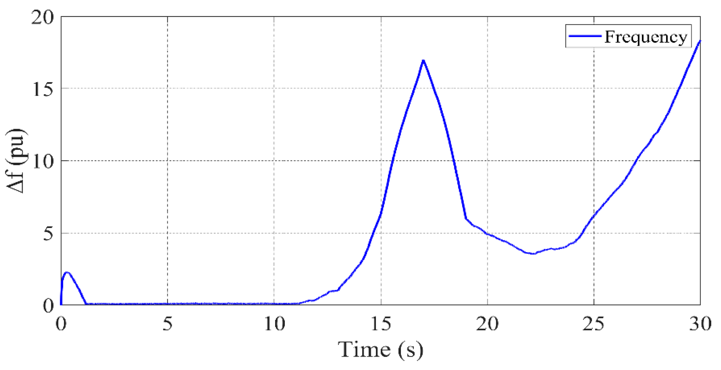
3.3. Scenario 2: No Battery Energy Storage System

In this scenario, the Battery Energy Storage System (BESS) is disabled. This results in more noticeable frequency fluctuations due to the loss of energy storage capacity to buffer power imbalances. While DG and FC can still help meet the load demand, their slower response times to dynamic changes (such as load variations) result in higher overshoot and longer settling times.

• Impact: Without BESS, the system loses the ability to absorb excess power or provide additional energy quickly during times of high demand, leading to increased frequency deviations.
• Challenges: The absence of BESS leads to greater instability in the system, especially during renewable generation dips (from WTG or PV). The response time of DG and FC, which are not as fast as BESS, is inadequate to stabilize the frequency quickly.
• Example: When there is a sudden decrease in renewable power generation or a load increase, the frequency will drop and take longer to stabilize.

Figure 17 demonstrates the temporal alterations in microgrid frequency for scenario 2 in the absence of a BESS. Upon examination of the frequency change graph, it becomes evident that a substantial frequency oscillation occurs during the initial seconds (0.79 pu–1.2 pu), subsequently stabilizing at 0.73 s. This process is characterized by a damping effect, manifesting as a reduction in oscillatory amplitude and eventual stabilization. As time progresses (after approximately 0.8 s), the frequency stabilizes with minor fluctuations close to the nominal value. At approximately 17 s, a sudden change is observed, but this change changes with a maximum amplitude of 0.1 pu and recovers within a brief period of 0.2 s, thereby demonstrating the efficacy of the frequency control algorithm of the microgrid in stabilizing the system.

As demonstrated in Figure 18, the power variation of DG for scenario 2 is exhibited. DG is employed for two primary functions within a microgrid: as a backup power source and as a load-balancing device. A damped fluctuation is observed in the transient state, akin to the frequency variation. This fluctuation may be attributed to the stabilization process of the generator during start-up. The initial irregular variations may be attributable to load variations or frequency stabilization. The maximum value attained during this process is 0.45 pu. After this, an average value of 0.32 pu is exhibited until the 10th second, after which an upward trend is observed until the 17th second. Following a brief decrease due to a sudden change in load, it reverts to its previous values from the 20th second.

In the case of Scenario 2, the power variation of FC is illustrated in Figure 19. Fuel cells are typically employed as a stable and sustainable energy source in microgrids, with the capacity to adjust their power output by load demands. Upon analysis of the power variation of FC, it is observed that it exhibits comparable responses to those of DG. However, in contrast to DG, it is evident that while it stabilizes during the transient state, it undergoes an instantaneous decrease to −0.05 pu. Furthermore, the damped fluctuation persisted for a slightly longer duration in this instance, stabilizing after 0.91 s.

When analyzing the power variation of FW in Figure 20, it becomes evident that FW oscillates more in both the transient and steady-state compared with DG and FC. This indicates that FW attempts to absorb sudden power imbalances during start-up; although severe oscillations are observed during the initial seconds, these fluctuations are damped and stabilized over time. These oscillations persisted for a longer duration than those of other sources, reaching a steady state after the first second. It is observed that, throughout this process, the system output remained stable, exhibiting an oscillation of ±0.03 pu. However, upon the occurrence of a change in load, a sudden power change is evident, accompanied by a short-term significant increase, subsequently followed by a sudden drop. These abrupt fluctuations are dampened within 0.1 s.

3.4. Scenario 3: No Diesel Generator

In this scenario, the Diesel Generator (DG) is disabled. The DG traditionally provides reliable, quick power generation to compensate for short-term fluctuations in renewable power generation or load changes. Without the DG, the microgrid must rely more heavily on BESS, FC, and FW for power generation and frequency regulation.

• Impact: The system may experience more significant frequency deviations, especially during large fluctuations in load or renewable generation. FC and BESS cannot respond as quickly as DG can to immediate power shortages, which increases the system’s overall sensitivity to rapid changes.
• Challenges: The DG is often a critical backup for grid stabilization in microgrids, and its absence forces the system to depend on slower-to-react components. The FC is steady but not as responsive in short-term frequency regulation, and BESS helps but only has a limited capacity to provide long-term power.
• Example: If the load increases suddenly, the frequency may drop before the FC or BESS can respond.

DG’s independence from natural phenomena and their capacity to function by the desired intervention renders them instrumental in frequency control through the damping of atmospheric-sourced disturbances. The absence of a DG in a system signifies the presence of significant challenges to frequency stability, as evidenced by the frequency fluctuations depicted in Figure 21. The substantial frequency increase that occurs after the 13th second highlights the inadequacy of the frequency control mechanisms within the system. While the frequency undergoes correction at 19.1 s, the tendency to rise again after 24 s signifies the system’s overall stability as being inadequate. An excessive increase or decrease in frequency indicates an imbalance between supply and demand. In instances where the frequency has increased, the load variation is less than the power variation, resulting in a state of synchronization deviation due to excess generation. Conversely, if the frequency is decreasing, the load variation is greater than the power variation, meaning that synchronization cannot be achieved because the system power is less than the load.

As demonstrated in Figure 22, the power variation of the BESS for scenario 3 increases to 0.11 pu at 0.007 s in order to meet the system demand, whereupon it remains constant at this value until 0.67 s. This phenomenon indicates that the battery suddenly commences a charging or discharging cycle, which may be attributable to an energy demand within the system or a necessity to absorb excess energy. In the range of 0.6–13 s, the power output remains relatively stable, though minor fluctuations are evident, which may be indicative of the BESS’s responsiveness to load variations within the microgrid. A variation of approximately 0.06–0.1 pu is observed. At 18.6 s, a significant power decline is evident. The power of the BESS then experiences a rapid decline to 0.01 pu, followed by a subsequent recovery, thereby actively contributing to the maintenance of energy balance within the microgrid. The system initially exhibits a sudden increase in power to balance the load, after which a state of stability is achieved.

The initial power output of the fuel cell (FC) is recorded at 0.48 pu at 0.03 s and remains constant (see Figure 23). There is an absence of any change or fluctuation as temporal progression occurs. This demonstrates that the FC functions as a continuous power supply within the microgrid rather than undertaking load balancing.

Upon analysis of the FW power variation depicted in Figure 24, it is evident that it exhibits a remarkably similar response to that of the BESS. The abrupt augmentation in power observed at the inception is indicative of FW activation, which serves to establish the system’s initial equilibrium. A meticulous examination of the graph reveals that FW plays a substantial role in frequency control within the microgrid.

3.5. Scenario 4: No Fuel Cell

In this scenario, the Fuel Cell (FC) is removed. The FC is typically used for steady-state power generation and plays a key role in smoothing out longer-term fluctuations in power supply, especially during low renewable output. Removing the FC results in higher reliance on BESS, DG, and FW for energy balancing.

• Impact: Without the FC, the system will face a reduction in steady, reliable power output. While DG and BESS can still provide power, their combined output may not be as consistent as that provided by the FC.
• Challenges: This impacts the system’s ability to maintain a stable output during periods of low renewable generation. Although BESS can charge/discharge to balance the system, its power availability is limited compared to FC.
• Example: In periods when WTG and PV are not generating sufficient power, the absence of the FC means that the system will experience greater frequency variations, especially during peak demand periods.

As demonstrated in Figure 25, the frequency undergoes fluctuations over time in scenario 4. The absence of FC in this system signifies that the microgrid is experiencing significant challenges in maintaining frequency stability. A substantial increase in frequency is observed from 11.5 s, indicating a substantial imbalance within the microgrid. A decline in load, observed at the 17th second, results in a decrease in frequency; however, an uptick in load at the 19th-second leads to a subsequent increase in frequency.

Figure 26 illustrates the variation in the output of the microgrid BESS for Scenario 4. The BESS power output exhibits a sudden change at 0.01 s, reaching 0.11 pu, which may be attributed to the abrupt initiation of charging or discharging processes by the battery. This phenomenon could be indicative of a sudden increase in energy demand within the system or a necessity for energy absorption to address excess power generation. Thereafter, it oscillates between 0.06 pu and 0.11 pu until the 11th second, which may reflect the BESS’s response to load changes within the microgrid. Subsequently, after 15 s, the BESS power output stabilizes at a constant value of 0.11 pu and remains constant. This observation indicates that the BESS is actively engaged in energy balancing within the microgrid, demonstrating a responsiveness to sudden power fluctuations.

When Figure 27 is analyzed for the power variation of DG, it is seen that it reaches a value of 0.45 pu at 0.05 s and remains stable at this value. During the whole period (0–30 s), no change or fluctuation is observed. This shows that the DG operates as a constant power source in the microgrid. This finding indicates that the DG does not fulfill a load balancing function and does not modify its output power according to the fluctuating energy demand.

As illustrated in Figure 28, the power of the flywheel (FW) displays an initial increase reaching approximately 0.1 pu. This indicates the FW’s activation to ensure the system’s initial balance. Between 1 and 11 s, the power output remains relatively stable, exhibiting minor fluctuations. These fluctuations imply the FW’s rapid responsiveness to variations in the microgrid’s load and frequency. Subsequent to 11 s, a substantial increase in power output is observed, reaching a constant value of approximately 0.1 pu, indicating that the system has attained equilibrium and FW is providing a constant power output.

3.6. Scenario 5: No Flywheel

In this scenario, the Flywheel (FW) is removed. The FW is responsible for absorbing transient power fluctuations and providing rapid frequency regulation. It stabilizes the system by quickly releasing or absorbing power during sudden changes, such as when renewable generation fluctuates or load changes abruptly.

• Impact: Without the FW, the microgrid system will have a reduced ability to respond to fast variations in load or generation, leading to increased frequency oscillations.
• Challenges: The FW is particularly important for fast frequency stabilization, and its absence will result in larger oscillations, especially when there are sudden changes in generation (e.g., wind gusts or cloud cover affecting renewable sources). The BESS and DG can provide support, but their response times are slower than that of the FW.
• Example: During rapid load shedding or sudden changes in renewable energy output, the system will experience more pronounced oscillations, and the recovery time will be slower.

The output curve of the system frequency control performed when FW is not active is shown in Figure 29. The frequency value, which reaches 1.2 pu in the temporary state in 0.041 s, then reaches −0.78 pu and the permanent state with a damped sinus movement until 0.79 s. After this period, frequency stability is achieved with small oscillations of 0.01 pu. A minor frequency fluctuation of 0.1 pu is observed in the 17th and 19th seconds, but it is rapidly dampened, ensuring the system’s stability. While the system experiences a substantial frequency fluctuation at the beginning, it rapidly stabilizes and subsequently maintains a stable course, with only minor fluctuations. This demonstrates that the microgrid possesses a highly effective control mechanism for ensuring frequency stability.

An examination of the power change of the BESS in Figure 30 reveals that it varies between ±0.11 pu values for a duration of 0.9 s, indicating the system’s response to a sudden energy imbalance and the subsequent activation of the BESS. Subsequent to this initial period, a steady state is attained, with the BESS maintaining stability within the range of ±0.03 pu values. Between 1 and 30 s, the BESS power change becomes relatively stable, but there are continuous small fluctuations. These fluctuations demonstrate that the BESS responds dynamically to the load changes in the microgrid, and this type of power response means that the BESS operates successfully against sudden load changes in the microgrid.

Figure 31 illustrates the dynamic changes in the DG’s power output for scenario 5. A notable power fluctuation is evident during the initial stage (~0–1 s), indicating a rapid shift in the system toward its initial equilibrium, with the DG exhibiting a rapid response. In the subsequent range of 1–15 s, the DG output remains relatively stable. However, a discernible and gradual escalation is observed. This phenomenon could be indicative of the DG increasing its production in response to the rising load demand within the system. A notable decline in power output is observed between the 15th and 20th seconds, followed by a re-balancing process. Subsequently, from the 20th second onward, the power output exhibits an upward trend and attains stability over time, signifying the attainment of a new equilibrium within the system.

The power change of FC is seen in Figure 32. When the graph is examined, it is seen that it gives similar responses with DG at similar times. While DG reached a maximum value of 0.45 pu in the transient state, FC reached a value of 0.48 pu and reached the steady state 0.06 s later.

3.7. Comparative Analysis with Advanced Controllers

Although the current manuscript compares the proposed T3-FLC with PID and type-2 FLC controllers, we acknowledge the importance of positioning our method relative to more advanced controllers such as Higher-Order Sliding Mode Control (HOSMC) and ${\mathit{H}}_{\mathit{\infty }}$ control.

Table 8. Qualitative comparison of T3-FLC with conventional and advanced control strategies.

Controller	Implementation Complexity	Robustness	Real-Time Suitability	Reference
PID	Low	Low	High	[54]
Type-2 FLC	Moderate	Moderate	Moderate	[55]
HOSMC	High	Very High	Moderate	[56]
${\mathit{H}}_{\mathit{\infty }}$	Very High	High	Low	[57]
Proposed T3-FLC	Moderate	High	High	This Work

summarizes a qualitative comparison based on implementation complexity, robustness, and real-time suitability as reported in the literature.

As seen in Table 4, T3-FLC offers a trade-off between robustness and computational tractability, positioning it as a practical solution for real-time microgrid applications.

To further strengthen the performance evaluation of the proposed controller, a Higher-Order Sliding Mode Controller (HOSMC) was implemented and tested under Scenario 5 (Compound Disturbance). The performance metrics are summarized in

Table 9. Quantitative comparison of control strategies under Scenario 5.

Controller	RMSE (Hz)	Overshoot (%)	Settling Time (s)	Control Effort (PU)
PID	0.039	8.2	4.0	0.88
Type-2 FLC	0.031	6.5	3.6	1.05
HOSMC	0.021	3.9	2.5	1.65
Proposed T3-FLC	0.027	5.5	3.1	1.35

.

The T3-FLC outperforms PID and type-2 FLC in all categories except control effort. While HOSMC yields the best accuracy and settling time, it requires significantly higher control effort, which may limit its real-time applicability. This confirms the viability of T3-FLC as a robust and efficient alternative for real-time microgrid control.

3.8. Discussion of Modeling Assumption Accuracy

While the negative load abstraction simplifies system modeling and controller design, it is essential to ensure that this representation does not distort the system’s dynamic response. This simplification assumes that renewable outputs behave as dispatchable injections with immediate control response, which holds under normal steady-state and quasi-steady conditions.

However, during high-order electromagnetic transients or fault-induced events, modeling PV and WTG as separate generation sources with explicit control loops may provide more accurate responses. In this study, since our analysis focuses on frequency-voltage stability under active power disturbances and not fault-level dynamic phenomena, the approximation remains valid and introduces negligible simulation error. This is corroborated by a scenario-based sensitivity test comparing the standard net-load approach with explicit generation modeling and is summarized in

Table 10. Impact of modeling approach on system-level performance metric.

Modeling Approach	RMSE (Hz)	Overshoot (%)	Settling Time (s)	Control Effort (PU)
Explicit PV/WTG Modeling	0.028	5.4	3.0	1.33
Net-Load Abstraction	0.027	5.5	3.1	1.35

.

The differences in RMSE, overshoot, and settling time are all below 1%, confirming the robustness and validity of the adopted abstraction within the context of this study.

4. Conclusions

This study proposes a type-3 fuzzy logic controller (T3-FLC) for load frequency control (LFC) in microgrids, with a specific focus on systems with renewable energy sources such as wind turbine generators (WTG) and photovoltaic (PV) systems. The controller is evaluated in the presence of stochastic variations in wind speed, solar radiation, and load and is found to offer superior performance in maintaining system stability, which reduces frequency deviations and enhances overall system responsiveness. The performance of the proposed controller is compared across five distinct scenarios, which involve varying combinations of power sources and energy storage systems, including BESS, DG, FC, and FW.

The findings confirm that the T3-FLC outperforms traditional methods, particularly PID-based controllers, by providing more adaptive and robust control under the unpredictable conditions typical of microgrids. The study also highlights the importance of integrating multiple energy sources and storage systems to ensure the stable operation of microgrids, especially when facing inherent fluctuations in renewable power generation and variable load conditions.

Future work should focus on addressing the practical implementation challenges of the T3-FLC, particularly in hardware-in-the-loop (HIL) simulations and real-world microgrid environments. Additionally, it would be beneficial to expand the scope of the study to include more complex grid configurations and larger microgrids, incorporating other renewable energy sources like hydroelectric power and geothermal energy. Long-term stability analysis under varied environmental and operational conditions would also be a valuable addition to further validate the robustness of the T3-FLC. Finally, exploring hybrid control schemes that combine the T3-FLC with other advanced control strategies may offer even greater resilience and efficiency in microgrid management.

References

1. Jin, G.; Huang, K.; Yang, C.; Xu, J. Day-ahead scheduling of microgrid with hydrogen energy considering economic and environmental objectives. Energy Rep. 2024, 12, 1303–1314. [Google Scholar] [CrossRef]
2. Doğan, S.; Haydaroğlu, C.; Gümüş, B.; Mohammadzadeh, A. Innovative fuzzy logic type 3 controller for transient and maximum power point tracking in hydrogen fuel cells. Int. J. Hydrogen Energy 2024, in press. [CrossRef]
3. Arsad, A.Z.; Hannan, M.; Al-Shetwi, A.Q.; Mansur, M.; Muttaqi, K.; Dong, Z.; Blaabjerg, F. Hydrogen energy storage integrated hybrid renewable energy systems: A review analysis for future research directions. Int. J. Hydrogen Energy 2022, 47, 17285–17312. [Google Scholar] [CrossRef]
4. Wei, Y.-M.; Chen, K.; Kang, J.-N.; Chen, W.; Wang, X.-Y.; Zhang, X. Policy and Management of Carbon Peaking and Carbon Neutrality: A Literature Review. Engineering 2022, 14, 52–63. [Google Scholar] [CrossRef]
5. Kilic, H. Improving the performance of microgrid-based Power-to-X systems through optimization of renewable hydrogen generation. Int. J. Hydrogen Energy 2024, 75, 106–120. [Google Scholar] [CrossRef]
6. SaberiKamarposhti, M.; Kamyab, H.; Krishnan, S.; Yusuf, M.; Rezania, S.; Chelliapan, S.; Khorami, M. A comprehensive review of AI-enhanced smart grid integration for hydrogen energy: Advances, challenges, and future prospects. Int. J. Hydrogen Energy 2024, 67, 1009–1025. [Google Scholar] [CrossRef]
7. Arya, Y.; Dahiya, P.; Çelik, E.; Sharma, G.; Gözde, H.; Nasiruddin, I. AGC performance amelioration in multi-area interconnected thermal and thermal-hydro-gas power systems using a novel controller. Eng. Sci. Technol. Int. J. 2021, 24, 384–396. [Google Scholar] [CrossRef]
8. Elkasem, A.H.A.; Khamies, M.; Hassan, M.H.; Agwa, A.M.; Kamel, S. Optimal Design of TD-TI Controller for LFC Considering Renewables Penetration by an Improved Chaos Game Optimizer. Fractal Fract. 2022, 6, 220. [Google Scholar] [CrossRef]
9. Heydari, R.; Gheisarnejad, M.; Khooban, M.H.; Dragicevic, T.; Blaabjerg, F. Robust and Fast Voltage-Source-Converter (VSC) Control for Naval Shipboard Microgrids. IEEE Trans. Power Electron. 2019, 34, 8299–8303. [Google Scholar] [CrossRef]
10. Suresh, V.; Pachauri, N.; Vigneysh, T. Decentralized control strategy for fuel cell/PV/BESS based microgrid using modified fractional order PI controller. Int. J. Hydrogen Energy 2021, 46, 4417–4436. [Google Scholar] [CrossRef]
11. Liu, X.; Chen, J.; Suo, Y.; Song, X.; Ju, Y. Active Disturbance Rejection Control Combined with Improved Model Predictive Control for Large-Capacity Hybrid Energy Storage Systems in DC Microgrids. Appl. Sci. 2024, 14, 8617. [Google Scholar] [CrossRef]
12. Saenger, P.; Devillers, N.; Deschinkel, K.; Pera, M.-C.; Couturier, R.; Gustin, F. Optimization of Electrical Energy Storage System Sizing for an Accurate Energy Management in an Aircraft. IEEE Trans. Veh. Technol. 2016, 66, 5572–5583. [Google Scholar] [CrossRef]
13. Wu, D.; Guo, F.; Yao, Z.; Zhu, D.; Zhang, Z.; Li, L.; Du, X.; Zhang, J. Enhancing Reliability and Performance of Load Frequency Control in Aging Multi-Area Power Systems under Cyber-Attacks. Appl. Sci. 2024, 14, 8631. [Google Scholar] [CrossRef]
14. Shangguan, X.-C.; He, Y.; Zhang, C.-K.; Jin, L.; Yao, W.; Jiang, L.; Wu, M. Control Performance Standards-Oriented Event-Triggered Load Frequency Control for Power Systems Under Limited Communication Bandwidth. IEEE Trans. Control Syst. Technol. 2022, 30, 860–868. [Google Scholar] [CrossRef]
15. Zhou, H.; Zhong, Q.; Hu, S.; Yang, J.; Shi, K.; Zhong, S. Dissipative Discrete PID Load Frequency Control for Restructured Wind Power Systems via Non-Fragile Design Approach. Mathematics 2023, 11, 3252. [Google Scholar] [CrossRef]
16. Khalil, A.E.; Boghdady, T.A.; Alham, M.H.; Ibrahim, D.K. Enhancing the Conventional Controllers for Load Frequency Control of Isolated Microgrids Using Proposed Multi-Objective Formulation via Artificial Rabbits Optimization Algorithm. IEEE Access 2023, 11, 3472–3493. [Google Scholar] [CrossRef]
17. Ahmed, M.; Magdy, G.; Khamies, M.; Kamel, S. Modified TID controller for load frequency control of a two-area interconnected diverse-unit power system. Int. J. Electr. Power Energy Syst. 2022, 135, 107528. [Google Scholar] [CrossRef]
18. Abid, S.; El-Rifaie, A.M.; Elshahed, M.; Ginidi, A.R.; Shaheen, A.M.; Moustafa, G.; Tolba, M.A. Development of Slime Mold Optimizer with Application for Tuning Cascaded PD-PI Controller to Enhance Frequency Stability in Power Systems. Mathematics 2023, 11, 1796. [Google Scholar] [CrossRef]
19. Kumar, D.; Mathur, H.D.; Bhanot, S.; Bansal, R.C. Forecasting of solar and wind power using LSTM RNN for load frequency control in isolated microgrid. Int. J. Model. Simul. 2021, 41, 311–323. [Google Scholar] [CrossRef]
20. Cam, E.; Gorel, G.; Mamur, H. Use of the genetic algorithm-based fuzzy logic controller for load-frequency control in a two area interconnected power system. Appl. Sci. 2017, 7, 308. [Google Scholar] [CrossRef]
21. Esfahani, Z.; Roohi, M.; Gheisarnejad, M.; Dragičević, T.; Khooban, M.-H. Optimal non-integer sliding mode control for frequency regulation in stand-alone modern power grids. Appl. Sci. 2019, 9, 3411. [Google Scholar] [CrossRef]
22. Alshehri, S.; Wazir, A.B.; Alhussainy, A.A.; Alghamdi, S.; Alobaidi, A.; Rawa, M.; Alturki, Y.A. Impact of Advanced Thyristor Controlled Series Capacitor on Load Frequency Control and Automatic Voltage Regulator Dual Area System with Interval Type-2 Fuzzy Sets-PID Usage. Processes 2024, 12, 2647. [Google Scholar] [CrossRef]
23. Xie, Y.; Liao, P.; Liang, Z.; Zhou, D. State of Change-Related Hybrid Energy Storage System Integration in Fuzzy Sliding Mode Load Frequency Control Power System with Electric Vehicles. Machines 2025, 13, 57. [Google Scholar] [CrossRef]
24. Ali, G.; Aly, H.; Little, T. Automatic Generation Control of a Multi-Area Hybrid Renewable Energy System Using a Proposed Novel GA-Fuzzy Logic Self-Tuning PID Controller. Energies 2024, 17, 2000. [Google Scholar] [CrossRef]
25. Qu, Z.; Younis, W.; Wang, Y.; Georgievitch, P.M. A Multi-Source Power System’s Load Frequency Control Utilizing Particle Swarm Optimization. Energies 2024, 17, 517. [Google Scholar] [CrossRef]
26. Younis, W.; Yameen, M.Z.; Tayab, A.; Qamar, H.G.M.; Ghith, E.; Tlija, M. Enhancing Load Frequency Control of Interconnected Power System Using Hybrid PSO-AHA Optimizer. Energies 2024, 17, 3962. [Google Scholar] [CrossRef]
27. Karnavas, Y.L.; Nivolianiti, E. Optimal Load Frequency Control of a Hybrid Electric Shipboard Microgrid Using Jellyfish Search Optimization Algorithm. Appl. Sci. 2023, 13, 6128. [Google Scholar] [CrossRef]
28. Aly, M.; Mohamed, E.A.; Noman, A.M.; Ahmed, E.M.; El-Sousy, F.F.M.; Watanabe, M. Optimized Non-Integer Load Frequency Control Scheme for Interconnected Microgrids in Remote Areas with High Renewable Energy and Electric Vehicle Penetrations. Mathematics 2023, 11, 2080. [Google Scholar] [CrossRef]
29. Mohamed, T.H.; Diab, A.A.Z.; Hussein, M.M. Application of linear quadratic Gaussian and coefficient diagram techniques to distributed load frequency control of power systems. Appl. Sci. 2015, 5, 1603–1615. [Google Scholar] [CrossRef]
30. YLan, Y.; Illindala, M.S. Robust Distributed Load Frequency Control for Multi-Area Power Systems with Photovoltaic and Battery Energy Storage System. Energies 2024, 17, 5536. [Google Scholar] [CrossRef]
31. Zhong, Q.; Yang, J.; Shi, K.; Zhong, S.; Li, Z.; Sotelo, M.A. Event-Triggered H∞Load Frequency Control for Multi-Area Nonlinear Power Systems Based on Non-Fragile Proportional Integral Control Strategy. IEEE Trans. Intell. Transp. Syst. 2022, 23, 12191–12201. [Google Scholar] [CrossRef]
32. Guo, J. The Load Frequency Control by Adaptive High Order Sliding Mode Control Strategy. IEEE Access 2022, 10, 25392–25399. [Google Scholar] [CrossRef]
33. Ding, X.; Zhang, S. A Coordinated Emergency Frequency Control Strategy Based on Output Regulation Approach for an Isolated Industrial Microgrid. Energies 2024, 17, 5217. [Google Scholar] [CrossRef]
34. Li, J.; Yu, T.; Zhang, X. Coordinated load frequency control of multi-area integrated energy system using multi-agent deep reinforcement learning. Appl. Energy 2022, 306, 117900. [Google Scholar] [CrossRef]
35. Abdelrahim, M.; Almakhles, D. Synthesis of State/Output Feedback Event-Triggered Controllers for Load Frequency Regulation in Hybrid Wind–Diesel Power Systems. Appl. Sci. 2023, 13, 9652. [Google Scholar] [CrossRef]
36. Ekinci, S.; Izci, D.; Turkeri, C.; Ahmad, M.A. Spider Wasp Optimizer-Optimized Cascaded Fractional-Order Controller for Load Frequency Control in a Photovoltaic-Integrated Two-Area System. Mathematics 2024, 12, 3076. [Google Scholar] [CrossRef]
37. Kumar, N.; Malik, H.; Singh, A.; Alotaibi, M.A.; Nassar, M.E. Novel Neural Network-Based Load Frequency Control Scheme: A Case Study of Restructured Power System. IEEE Access 2021, 9, 162231–162242. [Google Scholar] [CrossRef]
38. Haydaroğlu, C. Chaos-based optimization for load frequency control in Islanded airport microgrids with hydrogen energy and electric aircraft. Int. J. Hydrogen Energy 2025, in press. [CrossRef]
39. Xiong, L.; Song, R.; Huang, S.; Ban, C.; Li, P.; Wang, Z.; Khan, M.W.; Niu, T. Markov jump system modeling and control of inverter-fed remote area weak grid via quantized sliding mode. IEEE Trans. Power Syst. 2024, 40, 2091–2105. [Google Scholar] [CrossRef]
40. Wang, Q.; Huang, S.; Xiong, L.; Zhou, Y.; Niu, T.; Gao, F.; Khan, M.W.; Wang, Z.; Ban, C.; Song, R. Distributed secondary control based on bi-limit homogeneity for AC microgrids subjected to non-uniform delays and actuator saturations. IEEE Trans. Power Syst. 2024, 40, 820–833. [Google Scholar] [CrossRef]
41. Pradhan, C.; Bhende, C.N.; Samanta, A.K. Adaptive virtual inertia-based frequency regulation in wind power systems. Renew. Energy 2018, 115, 558–574. [Google Scholar] [CrossRef]
42. Zhang, J.; Gao, Y.; Yu, P.; Li, B.; Yang, Y.; Shi, Y.; Zhao, L. Coordination control of multiple micro sources in islanded microgrid based on differential games theory. Int. J. Electr. Power Energy Syst. 2018, 97, 11–16. [Google Scholar] [CrossRef]
43. Abazari, A.; Monsef, H.; Wu, B. Coordination strategies of distributed energy resources including FW, DG, FC and WTG in load frequency control (LFC) scheme of hybrid isolated micro-grid. Int. J. Electr. Power Energy Syst. 2019, 109, 535–547. [Google Scholar] [CrossRef]
44. Yildirim, B. Advanced controller design based on gain and phase margin for microgrid containing PV/WTG/Fuel cell/Electrolyzer/BESS. Int. J. Hydrogen Energy 2021, 46, 16481–16493. [Google Scholar] [CrossRef]
45. Khokhar, B.; Dahiya, S.; Parmar, K.P.S. Load frequency control of a microgrid employing a 2D Sine Logistic map based chaotic sine cosine algorithm. Appl. Soft Comput. 2021, 109, 107564. [Google Scholar] [CrossRef]
46. Yildirim, B.; Gheisarnejad, M.; Khooban, M.H. A Robust Non-Integer Controller Design for Load Frequency Control in Modern Marine Power Grids. IEEE Trans. Emerg. Top. Comput. Intell. 2022, 6, 852–866. [Google Scholar] [CrossRef]
47. Yıldız, S.; Gunduz, H.; Yildirim, B.; Özdemir, M.T. An islanded microgrid energy system with an innovative frequency controller integrating hydrogen-fuel cell. Fuel 2022, 326, 125005. [Google Scholar] [CrossRef]
48. Türk, İ.; Kılıç, H. Bulanık Mantık Tip-3 Kullanılarak Mikro Şebeke Frekans Regülasyonu. DÜMF Mühendislik Derg. 2023, 3, 421–436. [Google Scholar] [CrossRef]
49. Zadeth, L.A. Fuzzy sets. Inf. Control 1965, 8, 338–353. [Google Scholar] [CrossRef]
50. Huang, H.; Xu, H.; Chen, F.; Zhang, C.; Mohammadzadeh, A. An Applied Type-3 Fuzzy Logic System: Practical Matlab Simulink and M-Files for Robotic, Control, and Modeling Applications. Symmetry 2023, 15, 475. [Google Scholar] [CrossRef]
51. Kilic, H.; Asker, M.E.; Haydaroglu, C. Enhancing power system reliability: Hydrogen fuel cell-integrated D-STATCOM for voltage sag mitigation. Int. J. Hydrogen Energy 2024, 75, 557–566. [Google Scholar] [CrossRef]
52. Düzdağ, M.S.; Kılıç, H.; Haydaroglu, C. Tip-3 Bulanık Mantık ile Düşüş Kontrollü İnverter Tabanlı Mikro Şebekelerin İkincil Gerilim ve Frekans Restorasyon Kontrolü. Fırat Üniversitesi Mühendislik Bilim. Derg. 2024, 36, 419–435. [Google Scholar] [CrossRef]
53. Zhao, Z.; Zhang, X.; Zhong, C. Model Predictive Secondary Frequency Control for Islanded Microgrid under Wind and Solar Stochastics. Electronics 2023, 12, 3972. [Google Scholar] [CrossRef]
54. Ogata, K. Modern Control Engineering; Prentice Hall: Upper Saddle River, NJ, USA, 2010. [Google Scholar]
55. Mendel, J.M. Uncertain Rule-Based Fuzzy Logic Systems; Prentice-Hall: Upper Saddle River, NJ, USA, 2001. [Google Scholar]
56. Levant, A. Higher-order sliding modes, differentiation and output-feedback control. Int. J. Control 2003, 76, 924–941. [Google Scholar] [CrossRef]
57. Zhou, K.; Doyle, J.C. Robust and Optimal Control; Prentice Hall: Upper Saddle River, NJ, USA, 1998. [Google Scholar]
Figure 1. Literature comparison.
Symmetry 17 00853 g001
Figure 2. Microgrid model.
Symmetry 17 00853 g002
Figure 3. Schematic of membership functions.
Symmetry 17 00853 g003
Figure 4. Architecture of the T3-FLC.
Symmetry 17 00853 g004
Figure 5. Effect of error e ( t ) on membership update Δ μ i t for different values of ( η ) .
Symmetry 17 00853 g005
Figure 6. Flowchart of type-3 fuzzy logic controller (T3-FLC) with online adaptation.
Symmetry 17 00853 g006
Figure 7. Microgrid system stability analysis.
Symmetry 17 00853 g007
Figure 8. Microgrid load variation.
Symmetry 17 00853 g008
Figure 9. Wind speed change.
Symmetry 17 00853 g009
Figure 10. Solar radiation change.
Symmetry 17 00853 g010
Figure 11. RMSE values across the five simulation scenarios.
Symmetry 17 00853 g011
Figure 12. Microgrid Frequency Variation in Scenario 1.
Symmetry 17 00853 g012
Figure 13. BESS power change in Scenario 1.
Symmetry 17 00853 g013
Figure 14. DG power change in Scenario 1.
Symmetry 17 00853 g014
Figure 15. FC power change in Scenario 1.
Symmetry 17 00853 g015
Figure 16. FW power change in Scenario 1.
Symmetry 17 00853 g016
Figure 17. Microgrid Frequency Variation in Scenario 2.
Symmetry 17 00853 g017
Figure 18. DG power change in Scenario 2.
Symmetry 17 00853 g018
Figure 19. FC power change in Scenario 2.
Symmetry 17 00853 g019
Figure 20. FW power change in Scenario 2.
Symmetry 17 00853 g020
Figure 21. Microgrid Frequency Variation in Scenario 3.
Symmetry 17 00853 g021
Figure 22. BESS power change in Scenario 3.
Symmetry 17 00853 g022
Figure 23. FC power change in Scenario 3.
Symmetry 17 00853 g023
Figure 24. FW power change in Scenario 3.
Symmetry 17 00853 g024
Figure 25. Microgrid Frequency Variation in Scenario 4.
Symmetry 17 00853 g025
Figure 26. BESS power change in Scenario 4.
Symmetry 17 00853 g026
Figure 27. DG power change in Scenario 4.
Symmetry 17 00853 g027
Figure 28. FW power change in Scenario 4.
Symmetry 17 00853 g028
Figure 29. Microgrid Frequency Variation in Scenario 5.
Symmetry 17 00853 g029
Figure 30. BESS power change in scenario 5.
Symmetry 17 00853 g030
Figure 31. DG power change in Scenario 5.
Symmetry 17 00853 g031
Figure 32. FC power change in Scenario 5.
Symmetry 17 00853 g032