Hurwicz-Type Optimal Control Problem for Uncertain Singular Non-Causal Systems

Abstract

Uncertain singular non-causal systems represent a class of singular systems distinguished by the presence of regularity constraints and the involvement of uncertain variables. This paper considers optimal control problems for such systems under the Hurwicz criterion. By integrating dynamic programming with uncertainty theory, a recurrence equation is developed to address these problems. This equation has been shown to be effective in handling the optimal control problems of both linear and nonlinear uncertain singular non-causal systems, thereby enabling the derivation of analytical expressions for their corresponding optimal solutions. Moreover, the transformation of the original system into forward and backward subsystems reveals a fundamental temporal and structural symmetry, which significantly contributes to problem simplification. A detailed example is presented to illustrate the proposed results.

1. Introduction

Optimal control theory serves as a cornerstone of modern control theory, focusing on the systematic design of control strategies that optimize a specified performance criterion while satisfying predefined system constraints. Foundational contributions from Pontryagin’s maximum principle, Bellman’s dynamic programming, and Kalman’s filtering theory have collectively laid a solid foundation for the development of optimal control theory.

The development of optimal control has underscored the necessity of accurate system modeling for solving complex problems. Rosenbrock [1] revealed the limitations of traditional state-space models and introduced the concept of singular systems by incorporating singular matrices into dynamic coefficient matrices. In the field of economics, the dynamic input–output model proposed by Luenberger and Arbel [2] is classified as a singular system. Subsequently, Luenberger and Arbel [2] proposed a rigorous analytical framework to address the existence and uniqueness of solutions in both linear and nonlinear singular systems. Cobb [3] advanced the field further by establishing controllability and observability criteria, along with their duality principles, for singular systems within the context of structural system analysis. Building on these developments, Dai [4] systematically integrated optimal control theory with singular system theory, laying a comprehensive foundation for the optimal control of deterministic singular systems.

The study of systems influenced by various types of uncertainty is of vital importance to both systems science and optimal control theory. When uncertainty is modeled through random variables or Wiener processes, one arrives at stochastic systems [5,6,7], prompting the study of stochastic singular systems. For instance, Shu and Li [6] introduced dynamic programming into the analysis of optimal control problems involving stochastic singular systems, developing a recurrence equation framework based on probabilistic expectation. Vlasenko et al. [7] established conditions for the existence and uniqueness of solutions for a class of stochastic singular systems. Li and Ma [8] tackled the indefinite linear quadratic problem within singular Markov jump systems through the application of an equivalent transformation method.

The application of probability theory depends on the availability of sufficient historical data to construct probability distributions that approximate true frequencies. However, in many complex or emerging systems where sample data are sparse or nonexistent, expert judgment often serves as a key source of information. Due to the inherent conservatism and subjectivity of human cognition, expert assessments often deviate significantly from objective frequencies. Liu [9] argued that forcibly interpreting expert confidence using probabilistic frameworks can lead to paradoxical or counterintuitive conclusions—an insight that led directly to the development of [9,10]. Within the realm of uncertainty theory, uncertainties are modeled as uncertain variables, and expert assessments are expressed through uncertainty distributions. When system uncertainty is described using such uncertain variables, one obtains uncertain systems [11,12,13]. Zhu [14] demonstrated that solving optimality equations and recurrence equations can yield solutions to uncertain optimal control problems. This foundational work inspired a range of studies [15,16,17,18,19,20], which built the theoretical basis for analyzing uncertain singular systems. Shu and Zhu [21] proposed a rigorous analytical framework for analyzing the stability of uncertain singular systems. Under the uncertain expectation criterion, Shu et al. [22] developed a recurrence equation solution method for uncertain singular systems by introducing the assumptions of regularity and impulse-free conditions. Although the expectation criterion is widely adopted in uncertain optimization, its limitations are well recognized. For instance, in urban income distribution analysis, severe polarization may render average values misleading. To address such concerns, Shu and Zhu [23] applied the optimistic value criterion to uncertain singular systems, yielding several insightful results. Later, Chen et al. [24] investigated the linear–quadratic optimal control problem under the pessimistic value criterion. These developments in criterion design not only enrich the theoretical landscape of uncertain optimization but also offer new tools for addressing problems involving risk preferences and trade-offs. Recent research on the optimal control of uncertain singular systems has primarily focused on systems that are both regular and impulse-free [15,22,25]. While these studies have achieved significant progress, they encounter major challenges when extended to non-causal systems that satisfy only the regularity condition. Such non-causal systems frequently arise in practical applications, including certain problems in signal processing and electrical circuit analysis, where methods designed for causal and impulse-free systems may fail.

In this study, we extend the optimal control framework to regular but non-impulse-free uncertain singular non-causal systems by incorporating the Hurwicz criterion from decision theory. This criterion effectively balances risk and reward in uncertain environments, mirroring decision-making processes in investment scenarios where high-reward opportunities (optimistic values) must be weighed against potential losses (pessimistic values) using a weighting coefficient known as the Hurwicz index. For example, in smart grid dispatch, operators must balance the integration of renewable energy (optimistic objective) with the assurance of grid stability (pessimistic constraint). While previous work on causal uncertain singular systems is extensive [15,23], the distinctive nature of non-causal systems poses substantial obstacles to these established methods. To address this challenge, we adopt the algebraic transformation approach proposed in [26], which decomposes uncertain singular non-causal systems into forward and backward subsystems, fully exploiting their non-causal structure. This transformation simplifies the original problem into an equivalent form that is more amenable to analysis. In the context of the Hurwicz criterion, we analyze the properties of optimistic and pessimistic values and introduce a weighting coefficient to construct a unified objective function. Following an approach similar to [15], we employ a recurrence equation to solve this new class of uncertain optimal control problems. Our study not only generalizes existing results [15,23,26], but also broadens the scope of uncertain optimal control under mixed-risk evaluation criteria.

The remainder of this paper is organized as follows: Section 2 reviews the fundamental concepts of uncertainty theory and optimal control. Section 3 introduces a new modeling framework for uncertain singular non-causal systems, where the system is decomposed into forward and backward uncertain subsystems via an algebraic transformation method. Section 4 presents the formulation of a recurrence equation for solving the Hurwicz-type optimal control problem. Section 5 applies the recurrence equation to solve optimal control problems for both linear and nonlinear uncertain singular non-causal systems. Section 6 provides a numerical example to verify the effectiveness of the proposed approach.

2. Preliminaries

To facilitate the subsequent discussion, this section reviews fundamental concepts from uncertainty theory [10], followed by essential preliminaries on optimal control.

2.1. Uncertainty Theory

An uncertain variable $\xi$ defined on an uncertainty space $(\Gamma ,\mathcal{L},\mathcal{M})$ is associated with an uncertainty distribution $\mathsf{\Phi }\left(x\right)=\mathcal{M}\{\xi \le x\}$, $x\in \mathbb{R}$. The uncertain expectation of $\xi$ is given by

$$E_{\mathcal{M}}\left[\xi \right]={\int }_0^{+\infty }\mathcal{M}\{\xi \ge x\}dx-{\int }_{-\infty }^0\mathcal{M}\{\xi \le x\}dx={\int }_0^{+\infty }(1-\mathsf{\Phi }\left(x\right))dx-{\int }_{-\infty }^0\mathsf{\Phi }\left(x\right)dx.$$

This expectation is well defined as long as at least one of the two integrals is finite.

In addition to expectation, Liu [9] introduced two further metrics to characterize uncertain variables.

Definition 1

(Liu [9]). Given an uncertain variable ξ and a confidence level $\alpha \in (0,1]$, the α-optimistic value and α-pessimistic value of ξ are defined as

$${\xi }_{sup}\left(\alpha \right)=sup\{l\mid \mathcal{M}\{\xi \ge l\}\ge \alpha \},{\xi }_{inf}\left(\alpha \right)=inf\{l\mid \mathcal{M}\{\xi \le l\}\ge \alpha \},$$

respectively.

Lemma 1

(Liu [9]). Let ξ be an uncertain variable and $\rho \in \mathbb{R}$. Then, the following properties hold:

$${(\rho ·\xi )}_{sup}\left(\alpha \right)=\rho ·{\left(\xi \right)}_{sup}\left(\alpha \right),{(\rho ·\xi )}_{inf}\left(\alpha \right)=\rho ·{\left(\xi \right)}_{inf}\left(\alpha \right),$$

if $\rho \ge 0$, and

$${(\rho ·\xi )}_{sup}\left(\alpha \right)=\rho ·{\left(\xi \right)}_{inf}\left(\alpha \right),{(\rho ·\xi )}_{inf}\left(\alpha \right)=\rho ·{\left(\xi \right)}_{sup}\left(\alpha \right),$$

if $\rho <0$. For two independent uncertain variables ξ and η,

$${(\xi +\eta )}_{sup}\left(\alpha \right)={\left(\xi \right)}_{sup}\left(\alpha \right)+{\left(\eta \right)}_{sup}\left(\alpha \right),{(\xi +\eta )}_{inf}\left(\alpha \right)={\left(\xi \right)}_{inf}\left(\alpha \right)+{\left(\eta \right)}_{inf}\left(\alpha \right).$$

Under the uncertain measure $\mathcal{M}$, the expectation $E_{\mathcal{M}}\left[\xi \right]$ reflects the average tendency of $\xi$. Moreover, $\xi$ exceeds its $\alpha$-optimistic value with confidence level at least $\alpha$, and is less than or equal to its $\alpha$-pessimistic value with the same confidence level. As indicated by Lemma 1, the optimistic and pessimistic values are linearly additive for mutually independent uncertain variables. Specifically, uncertain variables ${\xi }_1,{\xi }_2,\dots ,{\xi }_k$ are said to be independent if, for any Borel sets ${\Lambda }_1,{\Lambda }_2,\dots ,{\Lambda }_k\subseteq \mathbb{R}$, the following condition holds:

$$\mathcal{M}\left\{\bigcap _{j=1}^k\{{\xi }_j\in {\Lambda }_j\}\right\}=\underset{1\le j\le k}{min}\mathcal{M}\{{\xi }_j\in {\Lambda }_j\}.$$

2.2. Optimal Control Problem

The central objective of uncertain optimal control is to determine control strategies that optimize the performance index of an uncertain system. Due to the presence of uncertain variables, such performance indices are typically evaluated using their numerical characteristics.

Zhu [14] proposed an optimal control framework based on the uncertain expectation

$$\begin{array}{c}\hfill \left\{\begin{array}{c}V(\mathit{y}\left(0\right),0)=\underset{\stackrel{\mathit{w}\left(j\right)\in \mathit{W}\left(j\right)}{0\le j\le J-1}}{max}{E}_{\mathcal{M}}\left[{\displaystyle \sum _{j=0}^{J-1}}\varphi (\mathit{y}\left(j\right),\mathit{w}\left(j\right),j)+\psi (\mathit{y}\left(J\right),J)\right]\hfill \\ \mathrm{s}.\mathrm{t}.\hfill \\ \mathit{y}(j+1)=\mathit{f}(\mathit{y}\left(j\right),\mathit{w}\left(j\right),{\mathit{\xi }}_j),\hfill \\ j=0,1,2,\cdots ,J-1,\hfill \end{array}\right.\end{array}$$

(1)

where $\mathit{y}\left(j\right)\in {\mathbb{R}}^m$ is the state, $\mathit{w}\left(j\right)\in {\mathbb{R}}^{n_w}$ is the control, and ${\mathit{\xi }}_j\in {\mathbb{R}}^{m_{\xi }}$ denotes an uncertain vector. $\mathit{f}:{\mathbb{R}}^m\times {\mathbb{R}}^{n_w}\times \mathbb{R}\to \mathbb{R}$ is a vector-valued function, and $\varphi$ and $\psi$ are real-valued functions. For each $k=J-1,J-2,\cdots ,1,0$, let $V\left(\mathit{y}\right(k),k)$ be the optimal value function from the k-th stage to the final stage. Then, we have the following equation:

$$\begin{array}{cc}\hfill & V(\mathit{y}\left(k\right),k)=\underset{\mathit{w}\left(k\right)\in \mathit{W}\left(k\right)}{max}{E}_{\mathcal{M}}\left[\varphi (\mathit{y}\left(k\right),\mathit{w}\left(k\right),k)+\sum _{j=K=1}^{J-1}\varphi (\mathit{y}\left(j\right),\mathit{w}\left(j\right),j)+\psi (\mathit{y}\left(J\right),J)\right],\hfill \end{array}$$

(2)

where ${\mathit{w}}^{*}(k+1),\cdots ,{\mathit{w}}^{*}(J-1)$ are optimal controls, and $V\left(\mathit{y}\right(J),J)=\psi \left(\mathit{y}\right(J),J)$.

The expectation is the average in the sense of the uncertain measure, which generally reflects the properties of uncertain variables well. However, in scenarios with highly skewed distributions or extreme polarization, reliance on the expectation may lead to misleading or suboptimal decisions. To address this limitation, Chen et al. [24] introduced an alternative formulation based on the pessimistic value:

$$\begin{array}{c}\hfill \left\{\begin{array}{c}V(\mathit{y}\left(0\right),0)=\underset{\stackrel{\mathit{w}\left(j\right)\in \mathit{W}\left(j\right)}{0\le j\le J-1}}{max}{\left[{\displaystyle \sum _{j=0}^{J-1}}\varphi (\mathit{y}\left(j\right),\mathit{w}\left(j\right),j)+\psi (\mathit{y}\left(J\right),J)\right]}_{inf}\left(\alpha \right)\hfill \\ \mathrm{s}.\mathrm{t}.\hfill \\ \mathit{y}(j+1)=\mathit{f}(\mathit{y}\left(j\right),\mathit{w}\left(j\right),{\mathit{\xi }}_j),\hfill \\ j=0,1,2,\cdots ,J-1,\hfill \end{array}\right.\end{array}$$

(3)

where $\alpha \in (0,1]$ is the confidence level. The corresponding recursive form is

$$\begin{array}{cc}\hfill & V(\mathit{y}\left(k\right),k)=\underset{\mathit{w}\left(k\right)\in \mathit{W}\left(k\right)}{max}{\left[\varphi (\mathit{y}\left(k\right),\mathit{w}\left(k\right),k)+\sum _{j=K=1}^{J-1}\varphi (\mathit{y}\left(j\right),\mathit{w}\left(j\right),j)+\psi (\mathit{y}\left(J\right),J)\right]}_{inf}\left(\alpha \right),\hfill \end{array}$$

(4)

to find the optimal controls of this problem.

Both optimal control problems (1) and (3) are established within the framework of standard systems. In contrast, the well-known Leontief dynamic input–output model belongs to the class of singular systems. The emergence of such non-causal singular models can be attributed to various physical considerations. For instance, in advanced signal processing, reconstructing complete signal information often requires accounting for future values, thereby necessitating non-causal models. Similarly, in circuit design, the output of components with memory effects may depend not only on past and present inputs but also on potential future inputs, motivating the development of non-causal system representations.

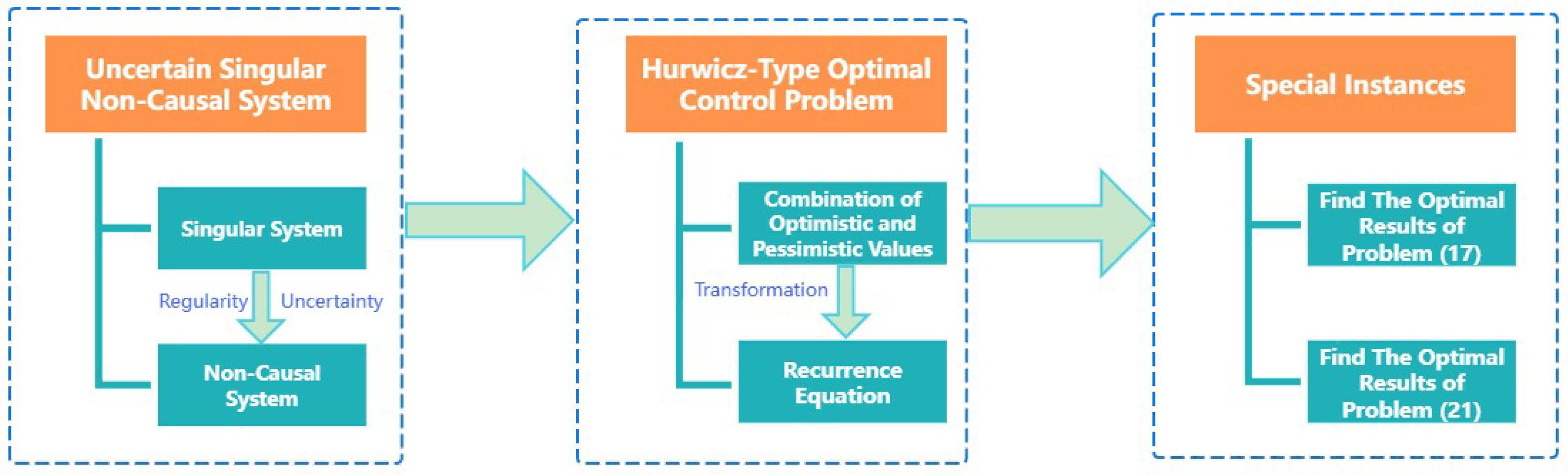
3. Uncertain Singular Non-Causal System

A class of linear singular systems was introduced by Dai [4] and is formulated as follows:

$$\begin{array}{c}\hfill \mathit{E}\mathit{y}(j+1)=\mathit{H}\mathit{y}\left(j\right)+\mathbf{\Pi }\mathit{w}\left(j\right),j=0,1,2,\cdots ,J-1.\end{array}$$

(5)

In this system, the state is represented by $\mathit{y}\left(j\right)\in {\mathbb{R}}^m$, and the control is denoted as $\mathit{w}\left(j\right)\in {\mathbb{R}}^{n_w}$. The matrices $\mathit{E},\mathit{H}\in {\mathbb{R}}^{m\times m}$ and $\mathbf{\Pi }\in {\mathbb{R}}^{m\times n_w}$ are deterministic. It is assumed that $rank\mathit{E}=q<m$.

Definition 2

(Dai [4]). The system (5) is called regular if $det(x\mathit{E}-\mathit{H}) \not\equiv 0$, where x is a complex variable, and $det(·)$ denotes the determinant of a matrix. The system (5) is impulse-free if $deg(det(x\mathit{E}-\mathit{H}\left)\right)=rank\mathit{E}$, where $deg(·)$ denotes the degree of the resulting polynomial.

From a physical perspective, the regularity condition ensures that the system model is mathematically well posed and physically meaningful. For singular systems such as (5), regularity ensures that the matrix pair $(\mathit{E},\mathit{A})$ does not yield purely algebraic equations, i.e., $det(x\mathit{E}-\mathit{H}) \not\equiv 0$. This avoids degenerate situations where the system’s dynamics are ill defined. For example, we consider a circuit with a capacitor and inductor in parallel, modeled by singular matrices due to algebraic constraints (e.g., Kirchhoff’s laws). The regularity condition ensures the circuit equations have a unique solution for voltages and currents over time, preventing contradictory constraints (e.g., infinite currents). If $det(x\mathit{E}-\mathit{H})\equiv 0$, the circuit would have no dynamic behavior, rendering it physically irrelevant. The impulse-free condition guarantees that the system does not generate impulsive responses (e.g., infinite spikes in states or controls) at initial time $j=0$. This is critical for practical systems, as impulses are unrealizable in hardware and can damage components. For instance, if a robotic arm undergoes a constrained motion with singular dynamics, an impulse-free system avoids instantaneous velocity jumps that could violate physical limitations.

Taking into account that the system (5) is subject to perturbations by uncertain vectors ${\mathit{\xi }}_0,{\mathit{\xi }}_1,\cdots ,{\mathit{\xi }}_{J-1}\in {\mathbb{R}}^{m_{\xi }}$, Shu and Zhu [15] proposed the following linear uncertain singular causal system, formulated within the framework of uncertainty theory:

$$\begin{array}{c}\hfill \mathit{E}\mathit{y}(j+1)=\mathit{H}\mathit{y}\left(j\right)+\mathbf{\Pi }\mathit{w}\left(j\right)+\mathit{D}{\mathit{\xi }}_j,j=0,1,2,\cdots ,J-1,\end{array}$$

(6)

where $(\mathit{E},\mathit{H})$ satisfies both the regularity and impulse-free conditions. In contrast, for an uncertain singular non-causal system, only the regularity condition is required. According to Definition 2, regularity is generally a less restrictive condition than the impulse-free condition. Notably, when an uncertain singular non-causal system also satisfies the impulse-free condition, it reduces to a causal system, as in (6).

Unlike previous research that mainly focused on linear uncertain singular causal systems, we presen nonlinear uncertain singular non-causal systems, which are a class of generalized systems that is worthy of investigation:

$$\begin{array}{c}\hfill \mathit{E}\mathit{y}(j+1)=\mathit{H}\mathit{y}\left(j\right)+\mathit{f}(\mathit{w}\left(j\right),{\mathit{\xi }}_j),j=0,1,2,\cdots ,J-1,\end{array}$$

(7)

where $(\mathit{E},\mathit{H})$ is regular, and $\mathit{f}:{\mathbb{R}}^{m_w}\times {\mathbb{R}}^{m_{\xi }}\to {\mathrm{R}}^m$ is a vector-valued function that satisfies the Lipschitz condition with respect to its arguments.

Lemma 2.

For the uncertain singular non-causal system (7), there exist non-singular matrices $\mathit{F}$ and $\mathit{M}$ such that the system is a restricted system equivalent to the following decoupled form:

$$\begin{array}{c}\hfill \left\{\begin{array}{c}{\overline{\mathit{y}}}_1(j+1)={\mathit{H}}_1{\overline{\mathit{y}}}_1\left(j\right)+{\mathit{f}}_1(\mathit{w}\left(j\right),{\mathit{\xi }}_j),\hfill \\ {\overline{\mathit{y}}}_2\left(j\right)={\mathit{E}}_2{\overline{\mathit{y}}}_2(j+1)-{\mathit{f}}_2(\mathit{w}\left(j\right),{\mathit{\xi }}_j),\hfill \\ j=0,1,2,\cdots ,J-1,\hfill \end{array}\right.\end{array}$$

(8)

with the coordinate transformation

$$\begin{array}{c}\hfill {\mathit{M}}^{-1}\mathit{y}\left(j\right)=\left[\begin{array}{c}{\overline{\mathit{y}}}_1\left(j\right)\\ {\overline{\mathit{y}}}_2\left(j\right)\end{array}\right],{\overline{\mathit{y}}}_1\left(j\right)\in {\mathbb{R}}^q,{\overline{\mathit{y}}}_2\left(j\right)\in {\mathbb{R}}^{m-q},\end{array}$$

and

$$\begin{array}{c}\hfill \mathit{F}\mathit{H}\mathit{M}=\left[\begin{array}{cc}{\mathit{H}}_1& \mathbf{0}\\ \mathbf{0}& {\mathbf{I}}_{m-q}\end{array}\right],\mathit{F}\mathit{f}(\mathit{w}\left(j\right),{\mathit{\xi }}_j)=\left[\begin{array}{c}{\mathit{f}}_1(\mathit{w}\left(j\right),{\mathit{\xi }}_j)\\ {\mathit{f}}_2(\mathit{w}\left(j\right),{\mathit{\xi }}_j)\end{array}\right],\end{array}$$

where ${\mathit{H}}_1\in {\mathbb{R}}^{q\times q},{\mathit{f}}_1(\mathit{w}\left(j\right),{\mathit{\xi }}_j)\in {\mathbb{R}}^q,{\mathit{f}}_2(\mathit{w}\left(j\right),{\mathit{\xi }}_j)\in {\mathbb{R}}^{(m-q)}$, ${\mathit{E}}_2\in {\mathbb{R}}^{(m-q)\times (m-q)}$ is a nilpotent matrix. The nilpotent index is denoted by $l_{min}=min\{l\mid {\mathit{E}}_2^l=\mathbf{0},l\in Z^{+}\}$.

Proof. 

As shown by Dai [4], there exist non-singular matrices $\mathit{F},\mathit{M}\in {\mathbb{R}}^{m\times m}$ such that

$$\begin{array}{c}\hfill \mathit{F}\mathit{E}\mathit{M}=\left[\begin{array}{cc}{\mathbf{I}}_q& \mathbf{0}\\ \mathbf{0}& {\mathit{E}}_2\end{array}\right].\end{array}$$

Applying this transformation to the system (7) yields the equivalent representation given in (8).

It is worth noting that both systems (7) and (8) share the same control. This transformation enables the analysis of associated optimal control problems through the simplified, decoupled system (8), enabling a more tractable analysis of system behavior under uncertainty.    □

4. Optimal Control Problem Based on the Hurwicz Criterion

Let $\varphi$ and $\psi$ be given measurable real-valued functions, and let $\alpha \in (0,1]$ denote the confidence level. The $\alpha$-optimistic and $\alpha$-pessimistic values of the uncertain variable

$$\sum _{j=0}^{J-1}\varphi (\mathit{y}\left(j\right),\mathit{w}\left(j\right),j)+\psi (\mathit{y}\left(J\right),J)$$

are defined, respectively, as

$${\left[\sum _{j=0}^{J-1}\varphi (\mathit{y}\left(j\right),\mathit{w}\left(j\right),j)+\psi (\mathit{y}\left(J\right),J)\right]}_{sup}\left(\alpha \right)$$

and

$${\left[\sum _{j=0}^{J-1}\varphi (\mathit{y}\left(j\right),\mathit{w}\left(j\right),j)+\psi (\mathit{y}\left(J\right),J)\right]}_{inf}\left(\alpha \right).$$

To unify these two evaluation criteria, we introduce a Hurwicz-type optimal control framework for the uncertain singular non-causal system (7). This framework balances the $\alpha$-optimistic and $\alpha$-pessimistic values using a weight parameter $\rho \in [0,1]$:

$$\begin{array}{c}\hfill \left\{\begin{array}{c}V(\mathit{y}\left(0\right),\mathit{y}\left(J\right),0)=\underset{\stackrel{\mathit{w}\left(j\right)\in \mathit{W}\left(j\right)}{0\le j\le J-1}}{max}\{\rho {\left[{\displaystyle \sum _{j=0}^{J-1}}\varphi (\mathit{y}\left(j\right),\mathit{w}\left(j\right),j)+\psi (\mathit{y}\left(J\right),J)\right]}_{sup}\left(\alpha \right)\hfill \\ +(1-\rho ){\left[{\displaystyle \sum _{j=0}^{J-1}}\varphi (\mathit{y}\left(j\right),\mathit{w}\left(j\right),j)+\psi (\mathit{y}\left(J\right),J)\right]}_{inf}\left(\alpha \right)\}\hfill \\ \mathrm{s}.\mathrm{t}.\hfill \\ \mathit{E}\mathit{y}(j+1)=\mathit{H}\mathit{y}\left(j\right)+\mathit{f}(\mathit{w}\left(j\right),{\mathit{\xi }}_j),\hfill \\ j=0,1,2,\cdots ,J-1.\hfill \end{array}\right.\end{array}$$

(9)

Remark 1.

In problem (9), the integration of two criteria forms a hybrid decision-making framework that accommodates the subjective preferences of decision-makers. The underlying rationale is rooted in the classical Hurwicz criterion [27], which enables a quantitative adjustment between optimism and pessimism via the introduction of a risk preference coefficient $\rho \in [0,1]$. Specifically, when $\rho =1$, it corresponds to a fully optimistic strategy, with decision-making focus on best-case outcomes, suitable for scenarios with abundant resource redundancy and high risk tolerance. Conversely, when $\rho =0$, the strategy is fully pessimistic, favoring absolute risk aversion and system robustness under worst-case scenarios, often observed in high-stakes environments. Intermediate values $(0<\rho <1)$ represent a balanced strategy, where linear weighting of the two extremes allows the decision-making process to flexibly reconcile performance and robustness, thereby addressing multidimensional requirements in practical engineering applications.

Lemma 3.

The problem (9) is equivalent to the following decomposed formulation:

$$\begin{array}{c}\hfill \left\{\begin{array}{c}V({\overline{\mathit{y}}}_1\left(0\right),{\overline{\mathit{y}}}_2\left(J\right),0)\hfill \\ =\underset{\stackrel{\mathit{w}\left(j\right)\in \mathit{W}\left(j\right)}{0\le j\le J-1}}{max}\{\rho {\left[{\displaystyle \sum _{j=0}^{J-1}}\overline{\varphi }({\overline{\mathit{y}}}_1\left(j\right),{\overline{\mathit{y}}}_2\left(J\right),\mathit{w}\left(j\right),\mathit{w}(j+1),\cdots ,\mathit{w}(J-1),j)+\overline{\psi }({\overline{\mathit{y}}}_1\left(J\right),{\overline{\mathit{y}}}_2\left(J\right),J)\right]}_{sup}\left(\alpha \right)\hfill \\ +(1-\rho ){\left[{\displaystyle \sum _{j=0}^{J-1}}\overline{\varphi }({\overline{\mathit{y}}}_1\left(j\right),{\overline{\mathit{y}}}_2\left(J\right),\mathit{w}\left(j\right),\mathit{w}(j+1),\cdots ,\mathit{w}(J-1),j)+\overline{\psi }({\overline{\mathit{y}}}_1\left(J\right),{\overline{\mathit{y}}}_2\left(J\right),J)\right]}_{inf}\left(\alpha \right)\}\hfill \\ s.t.\hfill \\ {\overline{\mathit{y}}}_1(j+1)={\mathit{H}}_1{\overline{\mathit{y}}}_1\left(j\right)+{\mathit{f}}_1(\mathit{w}\left(j\right),{\mathit{\xi }}_j),\hfill \\ {\overline{\mathit{y}}}_2\left(j\right)={\mathit{E}}_2{\overline{\mathit{y}}}_2(j+1)-{\mathit{f}}_2(\mathit{w}\left(j\right),{\mathit{\xi }}_j),\hfill \\ j=0,1,2,\cdots ,J-1,\hfill \end{array}\right.\end{array}$$

(10)

with $\mathit{M}=\left[{\mathit{M}}_1{\mathit{M}}_2\right],{\mathit{M}}_1\in {\mathbb{R}}^{m\times q},{\mathit{M}}_2\in {\mathbb{R}}^{m\times (m-q)}$, and

$$\begin{array}{cc}\hfill & \overline{\varphi }({\overline{\mathit{y}}}_1\left(j\right),{\overline{\mathit{y}}}_2\left(J\right),\mathit{w}\left(j\right),\mathit{w}(j+1),\cdots ,\mathit{w}(J-1),j)=\varphi ({\mathit{M}}_1{\overline{\mathit{y}}}_1\left(j\right)+{\mathit{M}}_2{\overline{\mathit{y}}}_2\left(j\right),\mathit{w}\left(j\right),j),\hfill \\ \hfill & \overline{\psi }({\overline{\mathit{y}}}_1\left(J\right),{\overline{\mathit{y}}}_2\left(J\right),j)=\psi ({\mathit{M}}_1{\overline{\mathit{y}}}_1\left(J\right)+{\mathit{M}}_2{\overline{\mathit{y}}}_2\left(J\right),J).\hfill \end{array}$$

The proof follows directly from Lemma 2.

Since the optimal value in (10) depends on the initial and terminal states, we denote it by $V(\overline{\mathit{y}}1\left(0\right),\overline{\mathit{y}}2\left(J\right),0)$. For any $k\in \{1,\dots ,J-1\}$, we define the value function given ${\overline{\mathit{y}}}_1\left(k\right)$ and ${\overline{\mathit{y}}}_2\left(J\right)$ as follows:

$$\begin{array}{c}\hfill \left\{\begin{array}{c}V({\overline{\mathit{y}}}_1\left(k\right),{\overline{\mathit{y}}}_2\left(J\right),k)\hfill \\ =\underset{\stackrel{\mathit{w}\left(j\right)\in \mathit{W}\left(j\right)}{k\le j\le J-1}}{max}\{\rho {\left[{\displaystyle \sum _{j=k}^{J-1}}\overline{\varphi }({\overline{\mathit{y}}}_1\left(j\right),{\overline{\mathit{y}}}_2\left(J\right),\mathit{w}\left(j\right),\mathit{w}(j+1),\cdots ,\mathit{w}(J-1),j)+\overline{\psi }({\overline{\mathit{y}}}_1\left(J\right),{\overline{\mathit{y}}}_2\left(J\right),J)\right]}_{sup}\left(\alpha \right)\hfill \\ +(1-\rho ){\left[{\displaystyle \sum _{j=k}^{J-1}}\overline{\varphi }({\overline{\mathit{y}}}_1\left(j\right),{\overline{\mathit{y}}}_2\left(J\right),\mathit{w}\left(j\right),\mathit{w}(j+1),\cdots ,\mathit{w}(J-1),j)+\overline{\psi }({\overline{\mathit{y}}}_1\left(J\right),{\overline{\mathit{y}}}_2\left(J\right),J)\right]}_{inf}\left(\alpha \right)\}\hfill \\ \mathrm{s}.\mathrm{t}.\hfill \\ {\overline{\mathit{y}}}_1(j+1)={\mathit{H}}_1{\overline{\mathit{y}}}_1\left(j\right)+{\mathit{f}}_1(\mathit{w}\left(j\right),{\mathit{\xi }}_j),\hfill \\ {\overline{\mathit{y}}}_2\left(j\right)={\mathit{E}}_2{\overline{\mathit{y}}}_2(j+1)-{\mathit{f}}_2(\mathit{w}\left(j\right),{\mathit{\xi }}_j),\hfill \\ j=k,k+1,k+2,\cdots ,J-1.\hfill \end{array}\right.\end{array}$$

The optimal solution can be obtained via the following recurrence relations.

Theorem 1.

For each $k=J-1,J-2,\cdots ,1,0$, the value function satisfies the following recurrence equation:

$$\begin{array}{cc}\hfill & V({\overline{\mathit{y}}}_1\left(k\right),{\overline{\mathit{y}}}_2\left(J\right),k)\hfill \\ & =\underset{\mathit{w}\left(k\right)\in \mathit{W}\left(k\right)}{max}\left\{\rho \right[\overline{\varphi }({\overline{\mathit{y}}}_1\left(k\right),{\overline{\mathit{y}}}_2\left(J\right),{\mathit{w}}^{*}\left(k\right),{\mathit{w}}^{*}(k+1),\cdots ,{\mathit{w}}^{*}(J-1),j)\hfill \\ & +\sum _{j=k+1}^{J-1}\overline{\varphi }({\overline{\mathit{y}}}_1\left(j\right),{\overline{\mathit{y}}}_2\left(J\right),{\mathit{w}}^{*}\left(j\right),{\mathit{w}}^{*}(j+1),\cdots ,{\mathit{w}}^{*}(J-1),j)+\overline{\psi }({\overline{\mathit{y}}}_1\left(J\right),{\overline{\mathit{y}}}_2\left(J\right),J){]}_{sup}\left(\alpha \right)\hfill \\ & +(1-\rho )[\overline{\varphi }({\overline{\mathit{y}}}_1\left(k\right),{\overline{\mathit{y}}}_2\left(J\right),{\mathit{w}}^{*}\left(k\right),{\mathit{w}}^{*}(k+1),\cdots ,{\mathit{w}}^{*}(J-1),j)\hfill \\ & +\sum _{j=k+1}^{J-1}\overline{\varphi }({\overline{\mathit{y}}}_1\left(j\right),{\overline{\mathit{y}}}_2\left(J\right),{\mathit{w}}^{*}\left(j\right),{\mathit{w}}^{*}(j+1),\cdots ,{\mathit{w}}^{*}(J-1),j)+\overline{\psi }({\overline{\mathit{y}}}_1\left(J\right),{\overline{\mathit{y}}}_2\left(J\right),J){]}_{inf}\left(\alpha \right)\},\hfill \end{array}$$

(11)

where ${\mathit{w}}^{*}(k+1),\cdots ,{\mathit{w}}^{*}(J-1)$ are optimal controls, and $V({\overline{\mathit{y}}}_1\left(J\right),{\overline{\mathit{y}}}_2\left(J\right),J)=\overline{\psi }({\overline{\mathit{y}}}_1\left(J\right),{\overline{\mathit{y}}}_2\left(J\right),J)$.

Proof. 

Let $\tilde{V}({\overline{\mathit{y}}}_1\left(k\right),{\overline{\mathit{y}}}_2\left(J\right),k)$ denote the right-hand side of the recurrence equation. By definition of the value function $V({\overline{\mathit{y}}}_1\left(k\right),{\overline{\mathit{y}}}_2\left(J\right),k)$, we have

$$\begin{array}{cc}\hfill & V({\overline{\mathit{y}}}_1\left(k\right),{\overline{\mathit{y}}}_2\left(J\right),k)\hfill \\ & \ge \rho {\left[\sum _{j=k}^{J-1}\overline{\varphi }({\overline{\mathit{y}}}_1\left(j\right),{\overline{\mathit{y}}}_2\left(J\right),\mathit{w}\left(j\right),\mathit{w}(j+1),\cdots ,\mathit{w}(J-1),j)+\overline{\psi }({\overline{\mathit{y}}}_1\left(J\right),{\overline{\mathit{y}}}_2\left(J\right),J)\right]}_{sup}\left(\alpha \right)\hfill \\ & +(1-\rho ){\left[\sum _{j=k}^{J-1}\overline{\varphi }({\overline{\mathit{y}}}_1\left(j\right),{\overline{\mathit{y}}}_2\left(J\right),\mathit{w}\left(j\right),\mathit{w}(j+1),\cdots ,\mathit{w}(J-1),j)+\overline{\psi }({\overline{\mathit{y}}}_1\left(J\right),{\overline{\mathit{y}}}_2\left(J\right),J)\right]}_{inf}\left(\alpha \right)\hfill \\ & =\rho [\overline{\varphi }({\overline{\mathit{y}}}_1\left(k\right),{\overline{\mathit{y}}}_2\left(J\right),\mathit{w}\left(k\right),\mathit{w}(k+1),\cdots ,\mathit{w}(J-1),j)\hfill \\ & +\sum _{j=k+1}^{J-1}\overline{\varphi }({\overline{\mathit{y}}}_1\left(j\right),{\overline{\mathit{y}}}_2\left(J\right),\mathit{w}\left(j\right),\mathit{w}(j+1),\cdots ,\mathit{w}(J-1),j)+\overline{\psi }({\overline{\mathit{y}}}_1\left(J\right),{\overline{\mathit{y}}}_2\left(J\right),J){]}_{sup}\left(\alpha \right)\hfill \\ & +[\overline{\varphi }({\overline{\mathit{y}}}_1\left(k\right),{\overline{\mathit{y}}}_2\left(J\right),\mathit{w}\left(k\right),\mathit{w}(k+1),\cdots ,\mathit{w}(J-1),j)\hfill \\ & +\sum _{j=k+1}^{J-1}\overline{\varphi }({\overline{\mathit{y}}}_1\left(j\right),{\overline{\mathit{y}}}_2\left(J\right),\mathit{w}\left(j\right),\mathit{w}(j+1),\cdots ,\mathit{w}(J-1),j)+\overline{\psi }({\overline{\mathit{y}}}_1\left(J\right),{\overline{\mathit{y}}}_2\left(J\right),J){]}_{sup}\left(\alpha \right)\hfill \\ & +(1-\rho )[\overline{\varphi }({\overline{\mathit{y}}}_1\left(k\right),{\overline{\mathit{y}}}_2\left(J\right),\mathit{w}\left(k\right),\mathit{w}(k+1),\cdots ,\mathit{w}(J-1),j)\hfill \\ & +\sum _{j=k+1}^{J-1}\overline{\varphi }({\overline{\mathit{y}}}_1\left(j\right),{\overline{\mathit{y}}}_2\left(J\right),\mathit{w}\left(j\right),\mathit{w}(j+1),\cdots ,\mathit{w}(J-1),j)+\overline{\psi }({\overline{\mathit{y}}}_1\left(J\right),{\overline{\mathit{y}}}_2\left(J\right),J){]}_{inf}\left(\alpha \right),\hfill \end{array}$$

(12)

Taking the maximum with respect to $\mathit{w}\left(j\right),j=k+1,k+2,\cdots ,J-1$ in (12), and then $\mathit{w}\left(k\right)$ in (12), we obtain

$$V({\overline{\mathit{y}}}_1\left(k\right),{\overline{\mathit{y}}}_2\left(J\right),k)\ge \tilde{V}({\overline{\mathit{y}}}_1\left(k\right),{\overline{\mathit{y}}}_2\left(J\right),k).$$

(13)

From another aspect, we have

$$\begin{array}{cc}\hfill & \rho {\left[\sum _{j=k}^{J-1}\overline{\varphi }({\overline{\mathit{y}}}_1\left(j\right),{\overline{\mathit{y}}}_2\left(J\right),\mathit{w}\left(j\right),\mathit{w}(j+1),\cdots ,\mathit{w}(J-1),j)+\overline{\psi }({\overline{\mathit{y}}}_1\left(J\right),{\overline{\mathit{y}}}_2\left(J\right),J)\right]}_{sup}\left(\alpha \right)\hfill \\ & +(1-\rho ){\left[\sum _{j=k}^{J-1}\overline{\varphi }({\overline{\mathit{y}}}_1\left(j\right),{\overline{\mathit{y}}}_2\left(J\right),\mathit{w}\left(j\right),\mathit{w}(j+1),\cdots ,\mathit{w}(J-1),j)+\overline{\psi }({\overline{\mathit{y}}}_1\left(J\right),{\overline{\mathit{y}}}_2\left(J\right),J)\right]}_{inf}\left(\alpha \right)\hfill \\ & \le \rho [\overline{\varphi }({\overline{\mathit{y}}}_1\left(k\right),{\overline{\mathit{y}}}_2\left(J\right),\mathit{w}\left(k\right),{\mathit{w}}^{*}(k+1),\cdots ,{\mathit{w}}^{*}(J-1),j)\hfill \\ & +\sum _{j=k+1}^{J-1}\overline{\varphi }({\overline{\mathit{y}}}_1\left(j\right),{\overline{\mathit{y}}}_2\left(J\right),{\mathit{w}}^{*}\left(j\right),{\mathit{w}}^{*}(j+1),\cdots ,{\mathit{w}}^{*}(J-1),j)+\overline{\psi }({\overline{\mathit{y}}}_1\left(J\right),{\overline{\mathit{y}}}_2\left(J\right),J){]}_{sup}\left(\alpha \right)\hfill \\ & +[\overline{\varphi }({\overline{\mathit{y}}}_1\left(k\right),{\overline{\mathit{y}}}_2\left(J\right),\mathit{w}\left(k\right),{\mathit{w}}^{*}(k+1),\cdots ,{\mathit{w}}^{*}(J-1),j)\hfill \\ & +\sum _{j=k+1}^{J-1}\overline{\varphi }({\overline{\mathit{y}}}_1\left(j\right),{\overline{\mathit{y}}}_2\left(J\right),{\mathit{w}}^{*}\left(j\right),{\mathit{w}}^{*}(j+1),\cdots ,{\mathit{w}}^{*}(J-1),j)+\overline{\psi }({\overline{\mathit{y}}}_1\left(J\right),{\overline{\mathit{y}}}_2\left(J\right),J){]}_{sup}\left(\alpha \right)\hfill \\ & +(1-\rho )[\overline{\varphi }({\overline{\mathit{y}}}_1\left(k\right),{\overline{\mathit{y}}}_2\left(J\right),\mathit{w}\left(k\right),{\mathit{w}}^{*}(k+1),\cdots ,{\mathit{w}}^{*}(J-1),j)\hfill \\ & +\sum _{j=k+1}^{J-1}\overline{\varphi }({\overline{\mathit{y}}}_1\left(j\right),{\overline{\mathit{y}}}_2\left(J\right),{\mathit{w}}^{*}\left(j\right),{\mathit{w}}^{*}(j+1),\cdots ,{\mathit{w}}^{*}(J-1),j)+\overline{\psi }({\overline{\mathit{y}}}_1\left(J\right),{\overline{\mathit{y}}}_2\left(J\right),J){]}_{inf}\left(\alpha \right),\hfill \\ \hfill & \le \underset{\mathit{w}\left(k\right)\in \mathit{W}\left(k\right)}{max}\left\{\rho \right[\overline{\varphi }({\overline{\mathit{y}}}_1\left(k\right),{\overline{\mathit{y}}}_2\left(J\right),{\mathit{w}}^{*}\left(k\right),{\mathit{w}}^{*}(k+1),\cdots ,{\mathit{w}}^{*}(J-1),j)\hfill \\ & +\sum _{j=k+1}^{J-1}\overline{\varphi }({\overline{\mathit{y}}}_1\left(j\right),{\overline{\mathit{y}}}_2\left(J\right),{\mathit{w}}^{*}\left(j\right),{\mathit{w}}^{*}(j+1),\cdots ,{\mathit{w}}^{*}(J-1),j)+\overline{\psi }({\overline{\mathit{y}}}_1\left(J\right),{\overline{\mathit{y}}}_2\left(J\right),J){]}_{sup}\left(\alpha \right)\hfill \\ & +[\overline{\varphi }({\overline{\mathit{y}}}_1\left(k\right),{\overline{\mathit{y}}}_2\left(J\right),{\mathit{w}}^{*}\left(k\right),{\mathit{w}}^{*}(k+1),\cdots ,{\mathit{w}}^{*}(J-1),j)\hfill \\ & +\sum _{j=k+1}^{J-1}\overline{\varphi }({\overline{\mathit{y}}}_1\left(j\right),{\overline{\mathit{y}}}_2\left(J\right),{\mathit{w}}^{*}\left(j\right),{\mathit{w}}^{*}(j+1),\cdots ,{\mathit{w}}^{*}(J-1),j)+\overline{\psi }({\overline{\mathit{y}}}_1\left(J\right),{\overline{\mathit{y}}}_2\left(J\right),J){]}_{sup}\left(\alpha \right)\hfill \\ & +(1-\rho )[\overline{\varphi }({\overline{\mathit{y}}}_1\left(k\right),{\overline{\mathit{y}}}_2\left(J\right),{\mathit{w}}^{*}\left(k\right),{\mathit{w}}^{*}(k+1),\cdots ,{\mathit{w}}^{*}(J-1),j)\hfill \\ & +\sum _{j=k+1}^{J-1}\overline{\varphi }({\overline{\mathit{y}}}_1\left(j\right),{\overline{\mathit{y}}}_2\left(J\right),{\mathit{w}}^{*}\left(j\right),{\mathit{w}}^{*}(j+1),\cdots ,{\mathit{w}}^{*}(J-1),j)+\overline{\psi }({\overline{\mathit{y}}}_1\left(J\right),{\overline{\mathit{y}}}_2\left(J\right),J){]}_{inf}\left(\alpha \right)\}\hfill \\ & =\tilde{V}({\overline{\mathit{y}}}_1\left(k\right),{\overline{\mathit{y}}}_2\left(J\right),k).\hfill \end{array}$$

(14)

Combining (13) and (14), we conclude that Equation (11) holds. Furthermore, for the terminal case $j=J$, it follows from the definition of $V({\overline{\mathit{y}}}_1\left(k\right),{\overline{\mathit{y}}}_2\left(J\right),k)$ that $V({\overline{\mathit{y}}}_1\left(J\right),{\overline{\mathit{y}}}_2\left(J\right),J)=\overline{\psi }({\overline{\mathit{y}}}_1\left(J\right),{\overline{\mathit{y}}}_2\left(J\right),J)$. This completes the proof.    □

Remark 2.

It is worth noting that when the matrix pair $(\mathit{E},\mathit{H})$ satisfies the regularity and impulse-free conditions, the problem (9) reduces to the optimal control problem for uncertain singular causal systems studied by Shu and Sheng [25]. Moreover, if the matrix $\mathit{E}$ is nonsingular, the problem (9) degenerates into an optimal control problem under the standard system framework:

$$\begin{array}{c}\hfill \left\{\begin{array}{c}V(\mathit{y}\left(0\right),\mathit{y}\left(J\right),0)=\underset{\stackrel{\mathit{w}\left(j\right)\in \mathit{W}\left(j\right)}{0\le j\le J-1}}{max}\{\rho {\left[{\displaystyle \sum _{j=0}^{J-1}}\varphi (\mathit{y}\left(j\right),\mathit{w}\left(j\right),j)+\psi (\mathit{y}\left(J\right),J)\right]}_{sup}\left(\alpha \right)\hfill \\ +(1-\rho ){\left[{\displaystyle \sum _{j=0}^{J-1}}\varphi (\mathit{y}\left(j\right),\mathit{w}\left(j\right),j)+\psi (\mathit{y}\left(J\right),J)\right]}_{inf}\left(\alpha \right)\}\hfill \\ s.t.\hfill \\ \mathit{y}(j+1)={\mathit{E}}^{-1}\mathit{H}\mathit{y}\left(j\right)+{\mathit{E}}^{-1}\mathit{f}(\mathit{w}\left(j\right),{\mathit{\xi }}_j),\hfill \\ j=0,1,2,\cdots ,J-1.\hfill \end{array}\right.\end{array}$$

(15)

In particular, when $\rho =0$, the problem becomes fully aligned with the optimal control problem under the pessimistic value criterion, as studied by Chen et al. [24]:

$$\begin{array}{c}\hfill \left\{\begin{array}{c}V(\mathit{y}\left(0\right),\mathit{y}\left(J\right),0)=\underset{\stackrel{\mathit{w}\left(j\right)\in \mathit{W}\left(j\right)}{0\le j\le J-1}}{max}\left\{{\left[{\displaystyle \sum _{j=0}^{J-1}}\varphi (\mathit{y}\left(j\right),\mathit{w}\left(j\right),j)+\psi (\mathit{y}\left(J\right),J)\right]}_{inf}\left(\alpha \right)\right\}\hfill \\ s.t.\hfill \\ \mathit{y}(j+1)={\mathit{E}}^{-1}\mathit{H}\mathit{y}\left(j\right)+{\mathit{E}}^{-1}\mathit{f}(\mathit{w}\left(j\right),{\mathit{\xi }}_j),\hfill \\ j=0,1,2,\cdots ,J-1.\hfill \end{array}\right.\end{array}$$

(16)

Consequently, the recurrence Equation (11) given in Theorem 1 simplifies to the form of Equation (4). These results collectively demonstrate that problem (9) developed in this work possesses a more general structural form, encompassing several well-established models as special cases.

This transformation simplifies the original optimal control problem (9), which involves an uncertain singular non-causal system, by reformulating it into the equivalent form (10). In this reformulation, the system is decomposed into a combination of forward and backward uncertain subsystems. Utilizing the recurrence equation, we are able to analyze problem (10) in a backward recursive fashion, starting from the terminal stage and proceeding step by step toward the initial stage. In this process, we assume that ${\mathit{\xi }}_0,{\mathit{\xi }}_1,\dots ,{\mathit{\xi }}_{J-1}$ are mutually independent. This assumption is introduced to facilitate the recursive computation by exploiting the linear additivity property of the optimistic and pessimistic values, as established in Lemma 1. Additionally, this recursive approach enables the derivation of analytical solutions for specific instances of optimal control problems involving uncertain singular non-causal systems.

5. Special Instances

First, we consider the following Hurwicz-type optimal control problem for a linear uncertain singular non-causal system:

$$\begin{array}{c}\hfill \left\{\begin{array}{c}V\left(\mathit{y}\right(0),\mathit{y}(J),0)\hfill \\ =\underset{\stackrel{\mathit{w}\left(j\right)\in {[-1,1]}^J}{0\le j\le J-1}}{max}\left\{\rho {\left[{\displaystyle \sum _{j=0}^{J-1}}{\mathit{\varphi }}_j^{\mathrm{T}}\mathit{y}\left(j\right)+{\mathit{\varphi }}_N^{\mathrm{T}}\mathit{y}\left(J\right)\right]}_{sup}\left(\alpha \right)+(1-\rho ){\left[{\displaystyle \sum _{j=0}^{J-1}}{\mathit{\varphi }}_j^{\mathrm{T}}\mathit{y}\left(j\right)+{\mathit{\varphi }}_N^{\mathrm{T}}\mathit{y}\left(J\right)\right]}_{inf}\left(\alpha \right)\right\}\hfill \\ \mathrm{s}.\mathrm{t}.\hfill \\ \mathit{E}\mathit{y}(j+1)=\mathit{H}\mathit{y}\left(j\right)+\mathbf{\Pi }\mathit{w}\left(j\right)+\mathit{D}{\mathit{\xi }}_j,\hfill \\ j=0,1,2,\cdots ,J-1,\hfill \end{array}\right.\end{array}$$

(17)

where ${\mathit{\varphi }}_j,{\mathit{\varphi }}_J\in {\mathbb{R}}^m,\mathbf{\Pi }\in {\mathbb{R}}^{m\times m_w},\mathit{D}\in {\mathbb{R}}^{m\times m_{\xi }}$. Let

$${\mathit{f}}_H\mathbf{\Pi }=\left[\begin{array}{c}{\mathbf{\Pi }}_1\\ {\mathbf{\Pi }}_2\end{array}\right],{\mathbf{\Pi }}_1\in {\mathbb{R}}^{q\times m_w},{\mathbf{\Pi }}_2\in {\mathbb{R}}^{(m-q)\times m_w},{\mathit{f}}_H\mathit{D}=\left[\begin{array}{c}{\mathit{D}}_1\\ {\mathit{D}}_2\end{array}\right],{\mathit{D}}_1\in {\mathbb{R}}^{q\times m_{\xi }},{\mathit{D}}_2\in {\mathbb{R}}^{(m-q)\times m_{\xi }}.$$

If we assume that ${\mathit{D}}_2=\mathbf{0}$, then problem (17) is equivalent to the following transformed problem:

$$\begin{array}{c}\hfill \left\{\begin{array}{c}V({\overline{\mathit{y}}}_1\left(0\right),{\overline{\mathit{y}}}_2\left(J\right),0)\hfill \\ =\underset{\stackrel{\mathit{w}\left(j\right)\in {[-1,1]}^{n_w}}{0\le j\le J-1}}{max}\{\rho {\left[{\displaystyle \sum _{j=0}^{J-1}}{\mathit{\varphi }}_j^{\mathrm{T}}[{\mathit{M}}_1{\overline{\mathit{y}}}_1\left(j\right)+{\mathit{M}}_2{\overline{\mathit{y}}}_2\left(j\right)]+{\mathit{\varphi }}_J^{\mathrm{T}}[{\mathit{M}}_1{\overline{\mathit{y}}}_1\left(J\right)+{\mathit{M}}_2{\overline{\mathit{y}}}_2\left(J\right)]\right]}_{sup}\left(\alpha \right)\hfill \\ +(1-\rho ){\left[{\displaystyle \sum _{j=0}^{J-1}}{\mathit{\varphi }}_j^{\mathrm{T}}[{\mathit{M}}_1{\overline{\mathit{y}}}_1\left(j\right)+{\mathit{M}}_2{\overline{\mathit{y}}}_2\left(j\right)]+{\mathit{\varphi }}_J^{\mathrm{T}}[{\mathit{M}}_1{\overline{\mathit{y}}}_1\left(J\right)+{\mathit{M}}_2{\overline{\mathit{y}}}_2\left(J\right)]\right]}_{inf}\left(\alpha \right)\}\hfill \\ \mathrm{s}.\mathrm{t}.\hfill \\ {\overline{\mathit{y}}}_1(j+1)={\mathit{H}}_1{\overline{\mathit{y}}}_1\left(j\right)+{\mathbf{\Pi }}_1\mathit{w}\left(j\right)+{\mathit{D}}_1{\mathit{\xi }}_j,\hfill \\ {\overline{\mathit{y}}}_2\left(j\right)={\mathit{E}}_2{\overline{\mathit{y}}}_2(j+1)-{\mathbf{\Pi }}_2\mathit{w}\left(j\right),\hfill \\ j=0,1,2,\cdots ,J-1.\hfill \end{array}\right.\end{array}$$

(18)

Theorem 2.

The optimal controls ${\mathit{w}}^{*}\left(j\right)$ for the problem (18) are

$$\begin{array}{c}\hfill w_{i_w}^{*}\left(j\right)=\left\{\begin{array}{cc}sign\left\{l_{i_w}^j\right\},\hfill & if l_{i_w}^j\ne 0,\hfill \\ sign\left\{u_{i_w}^{j,1}\right\},\hfill & if l_{i_w}^j=0,and{u}_{i_w}^{j,1}\ne 0,\hfill \\ sign\left\{u_{i_w}^{j,1}\right\},\hfill & if l_{i_w}^j=0,u_{i_w}^{j,1}=0,and{u}_{i_w}^{j,2}\ne 0\hfill \\ \dots \hfill \\ sign\left\{u_{i_w}^{j,j}\right\},\hfill & if l_{i_w}^j=0,u_{i_w}^{j,1}=0,\cdots ,u_{i_w}^{j,j-1}=0,and{u}_{i_w}^{j,j}\ne 0\hfill \\ undetermined,\hfill & if l_{i_w}^j=0,u_{i_w}^{j,1}=0,\cdots ,u_{i_w}^{j,j-1}=0,and{u}_{i_w}^{j,j}=0,\hfill \end{array}\right.\end{array}$$

(19)

where

$${\mathit{l}}^j={\mathit{r}}_{j+1}^{\mathrm{T}}{\mathbf{\Pi }}_1-{\mathit{\varphi }}_j^{\mathrm{T}}{\mathit{M}}_2{\mathbf{\Pi }}_2,{\mathit{u}}^{j,{\tilde{l}}_w}=-\sum _{k=1}^{{\tilde{l}}_w}{\mathit{\varphi }}_{j-k}^{\mathrm{T}}{\mathit{M}}_2{\mathit{E}}_2^k{\mathbf{\Pi }}_2,$$

(20)

and

$${\mathit{r}}_j^{\mathrm{T}}={\mathit{\varphi }}_j^{\mathrm{T}}{\mathit{M}}_1+{\mathit{r}}_{j+1}^{\mathrm{T}}{\mathit{H}}_1,$$

(21)

for $i_w=1,2,\cdots ,n_w,{\tilde{l}}_w=1,2,\cdots ,j,j=1,2,\cdots ,J-1$. The optimal values are

$$\begin{array}{cc}\hfill & V({\overline{\mathit{y}}}_1\left(J\right),{\overline{\mathit{y}}}_2\left(J\right),J)={\mathit{r}}_J^{\mathrm{T}}{\overline{\mathit{y}}}_1\left(J\right)+{\mathit{s}}_J^{\mathrm{T}}{\overline{\mathit{y}}}_2\left(J\right),\hfill \end{array}$$

(22)

$$\begin{array}{cc}\hfill & V({\overline{\mathit{y}}}_1\left(j\right),{\overline{\mathit{y}}}_2\left(J\right),j)={\mathit{r}}_j^{\mathrm{T}}{\overline{\mathit{y}}}_1\left(j\right)+{\mathit{s}}_j^{\mathrm{T}}{\overline{\mathit{y}}}_2\left(J\right)+\sum _{k=j+1}^{J-1}{\mathit{u}}^{k,k-j}{\mathit{w}}^{*}\left(k\right)+\sum _{k=j}^{J-1}\mid \mid {\mathit{l}}^k\mid {\mid }_1+\sum _{k=j}^{J-1}{t}_k,\hfill \end{array}$$

(23)

where

$${\mathit{s}}_j^{\mathrm{T}}={\mathit{\varphi }}_j^{\mathrm{T}}{\mathit{M}}_2{\mathit{E}}_2^{J-j}+{\mathit{s}}_{j+1}^{\mathrm{T}},t_k=\rho {\left[{\mathit{r}}_{k+1}^{\mathrm{T}}{\mathit{D}}_1{\mathit{\xi }}_k\right]}_{sup}\left(\alpha \right)+(1-\rho ){\left[{\mathit{r}}_{k+1}^{\mathrm{T}}{\mathit{D}}_1{\mathit{\xi }}_k\right]}_{inf}\left(\alpha \right),$$

(24)

for $k=j,j+1,\cdots ,J-1,j=0,1,2,\cdots ,J-1$, with ${\mathit{r}}_J^{\mathrm{T}}={\mathit{\varphi }}_J^{\mathrm{T}}{\mathit{M}}_1$, ${\mathit{s}}_J^{\mathrm{T}}={\mathit{\varphi }}_J^{\mathrm{T}}{\mathit{M}}_2$.

Proof. 

According to Theorem 1, it is shown that $V({\mathit{y}}_1\left(J\right),{\mathit{y}}_2\left(J\right),J)={\mathit{r}}_J^{\mathrm{T}}{\overline{\mathit{y}}}_1\left(J\right)+{\mathit{s}}_J^{\mathrm{T}}{\overline{\mathit{y}}}_2\left(J\right)$, where ${\mathit{r}}_J^{\mathrm{T}}={\mathit{\varphi }}_J^{\mathrm{T}}{\mathit{M}}_1$ and ${\mathit{s}}_J^{\mathrm{T}}={\mathit{\varphi }}_J^{\mathrm{T}}{\mathit{M}}_2$. When $j=J-1$, by applying Theorem 1, we have

$$\begin{array}{cc}\hfill & V({\mathit{y}}_1(J-1),{\mathit{y}}_2(J-1),J-1)\hfill \\ \hfill & =\underset{\mathit{w}(J-1)\in {[-1,1]}^{n_w}}{max}\{\rho {[{\mathit{\varphi }}_{J-1}^{\mathrm{T}}({\mathit{M}}_1{\overline{\mathit{y}}}_1(J-1)+{\mathit{M}}_2{\overline{\mathit{y}}}_2(J-1))+{\mathit{r}}_J^{\mathrm{T}}{\overline{\mathit{y}}}_1\left(J\right)+{\mathit{s}}_J^{\mathrm{T}}{\overline{\mathit{y}}}_2\left(J\right)]}_{sup}\left(\alpha \right)\hfill \\ \hfill & +(1-\rho ){[{\mathit{\varphi }}_{J-1}^{\mathrm{T}}({\mathit{M}}_1{\overline{\mathit{y}}}_1(J-1)+{\mathit{M}}_2{\overline{\mathit{y}}}_2(J-1))+{\mathit{r}}_J^{\mathrm{T}}{\overline{\mathit{y}}}_1\left(J\right)+{\mathit{s}}_J^{\mathrm{T}}{\overline{\mathit{y}}}_2\left(J\right)]}_{inf}\left(\alpha \right)\}\hfill \\ \hfill & =\underset{\mathit{w}(J-1)\in {[-1,1]}^{n_w}}{max}\left\{\rho \right[{\mathit{\varphi }}_{J-1}^{\mathrm{T}}[{\mathit{M}}_1{\overline{\mathit{y}}}_1(J-1)+{\mathit{M}}_2({\mathit{E}}_2{\overline{\mathit{y}}}_2\left(J\right)-{\mathbf{\Pi }}_2\mathit{w}(J-1))]\hfill \\ & +{\mathit{r}}_J^{\mathrm{T}}({\mathit{H}}_1{\overline{\mathit{y}}}_1(J-1)+{\mathbf{\Pi }}_1\mathit{w}(J-1)+{\mathit{D}}_1{\mathit{\xi }}_{J-1})+{\mathit{s}}_J^{\mathrm{T}}{\overline{\mathit{y}}}_2\left(J\right){]}_{sup}\left(\alpha \right)\hfill \\ & +(1-\rho )[{\mathit{\varphi }}_{J-1}^{\mathrm{T}}[{\mathit{M}}_1{\overline{\mathit{y}}}_1(J-1)+{\mathit{M}}_2({\mathit{E}}_2{\overline{\mathit{y}}}_2\left(J\right)-{\mathbf{\Pi }}_2\mathit{w}(J-1))]\hfill \\ & +{\mathit{r}}_J^{\mathrm{T}}({\mathit{H}}_1{\overline{\mathit{y}}}_1(J-1)+{\mathbf{\Pi }}_1\mathit{w}(J-1)+{\mathit{D}}_1{\mathit{\xi }}_{J-1})+{\mathit{s}}_J^{\mathrm{T}}{\overline{\mathit{y}}}_2\left(J\right){]}_{inf}\left(\alpha \right)\}\hfill \\ \hfill & =({\mathit{\varphi }}_{J-1}^{\mathrm{T}}{\mathit{M}}_1+{\mathit{r}}_J^{\mathrm{T}}{\mathit{H}}_1){\overline{\mathit{y}}}_1(J-1)+({\mathit{\varphi }}_{J-1}^{\mathrm{T}}{\mathit{M}}_2{\mathit{E}}_2+{\mathit{s}}_J^{\mathrm{T}}){\overline{\mathit{y}}}_2\left(J\right)\hfill \\ & +\underset{\mathit{w}(J-1)\in {[-1,1]}^{n_w}}{max}\left[({\mathit{r}}_J^{\mathrm{T}}{\mathbf{\Pi }}_1-{\mathit{\varphi }}_{J-1}^{\mathrm{T}}{\mathit{M}}_2{\mathbf{\Pi }}_2)\mathit{w}(J-1)\right]+\rho {\left[{\mathit{r}}_J^{\mathrm{T}}{\mathit{D}}_1{\mathit{\xi }}_{J-1}\right]}_{sup}\left(\alpha \right)+(1-\rho ){\left[{\mathit{r}}_J^{\mathrm{T}}{\mathit{D}}_1{\mathit{\xi }}_{J-1}\right]}_{inf}\left(\alpha \right).\hfill \end{array}$$

Let ${\mathit{l}}^{J-1}={\mathit{r}}_J^{\mathrm{T}}{\mathbf{\Pi }}_1-{\mathit{\varphi }}_{J-1}^{\mathrm{T}}{\mathit{M}}_2{\mathbf{\Pi }}_2$. For each $i_w=1,2,\cdots ,n_w$, we obtain

$$\begin{array}{c}\hfill w_{i_w}^{*}(J-1)=\left\{\begin{array}{cc}sign\left\{l_{i_w}^{J-1}\right\},\hfill & if l_{i_w}^{J-1}\ne 0,\hfill \\ undetermined,\hfill & if l_{i_w}^{J-1}=0,\hfill \end{array}\right.\end{array}$$

where $l_{i_w}^{J-1}$ represents the $i_w$-th element of the vector. Denote the 1-norm of the vector ${\mathit{l}}^{J-1}$ as $\mid \mid {\mathit{l}}^{J-1}\mid {\mid }_1$; then,

$$\begin{array}{c}\hfill V({\overline{\mathit{y}}}_1(J-1),{\overline{\mathit{y}}}_2\left(J\right),J-1)={\mathit{r}}_{J-1}^{\mathrm{T}}{\overline{\mathit{y}}}_1(J-1)+{\mathit{s}}_{J-1}^{\mathrm{T}}{\overline{\mathit{y}}}_2\left(J\right)+\mid \mid {\mathit{l}}^{J-1}\mid {\mid }_1+t_{J-1},\end{array}$$

where

$$\begin{array}{cc}\hfill & {\mathit{r}}_{J-1}^{\mathrm{T}}={\mathit{\varphi }}_{J-1}^{\mathrm{T}}{\mathit{M}}_1+{\mathit{r}}_J^{\mathrm{T}}{\mathit{H}}_1,{\mathit{s}}_{J-1}^{\mathrm{T}}={\mathit{\varphi }}_{J-1}^{\mathrm{T}}{\mathit{M}}_2{\mathit{E}}_2+{\mathit{s}}_J^{\mathrm{T}},\hfill \\ & t_{J-1}=\rho {\left[{\mathit{r}}_J^{\mathrm{T}}{\mathit{D}}_1{\mathit{\xi }}_{J-1}\right]}_{sup}\left(\alpha \right)+(1-\rho ){\left[{\mathit{r}}_J^{\mathrm{T}}{\mathit{D}}_1{\mathit{\xi }}_{J-1}\right]}_{inf}\left(\alpha \right).\hfill \end{array}$$

At this point, when considering the case of $j=J-2$, we are able to obtain the subsequent outcome by leveraging Theorem 1:

$$\begin{array}{cc}\hfill & V({\mathit{y}}_1(J-2),{\mathit{y}}_2\left(J\right),J-2)\hfill \\ \hfill & =\underset{\mathit{w}(J-2)\in {[-1,1]}^{n_w}}{max}\left\{\rho \right[{\mathit{\varphi }}_{J-2}^{\mathrm{T}}{[{\mathit{M}}_1{\overline{\mathit{y}}}_1(J-2)+{\mathit{M}}_2{\overline{\mathit{y}}}_2(J-2)]}_{sup}\left(\alpha \right)\hfill \\ & +{\mathit{r}}_{J-1}^{\mathrm{T}}{\overline{\mathit{y}}}_1(J-1)+{\mathit{s}}_{J-1}^{\mathrm{T}}{\overline{\mathit{y}}}_2\left(J\right)+\mid \mid {\mathit{l}}^{J-1}\mid {\mid }_1+t_{J-1}{]}_{sup}\left(\alpha \right)\hfill \\ & +(1-\rho )[{\mathit{\varphi }}_{J-2}^{\mathrm{T}}{[{\mathit{M}}_1{\overline{\mathit{y}}}_1(J-2)+{\mathit{M}}_2{\overline{\mathit{y}}}_2(J-2)]}_{sup}\left(\alpha \right)\hfill \\ & +{\mathit{r}}_{J-1}^{\mathrm{T}}{\overline{\mathit{y}}}_1(J-1)+{\mathit{s}}_{J-1}^{\mathrm{T}}{\overline{\mathit{y}}}_2\left(J\right)+\mid \mid {\mathit{l}}^{J-1}\mid {\mid }_1+t_{J-1}{]}_{inf}\left(\alpha \right)\}\hfill \\ \hfill & =\underset{\mathit{w}(J-2)\in {[-1,1]}^{n_w}}{max}\left\{\rho \right[{\mathit{\varphi }}_{J-2}^{\mathrm{T}}[{\mathit{M}}_1{\overline{\mathit{y}}}_1(J-2)+{\mathit{M}}_2({\mathit{E}}_2^2{\overline{\mathit{y}}}_2\left(J\right)-{\mathbf{\Pi }}_2\mathit{w}(J-2)-{\mathit{E}}_2{\mathbf{\Pi }}_2{\mathit{w}}^{*}(J-1))]\hfill \\ & +{\mathit{r}}_{J-1}^{\mathrm{T}}({\mathit{H}}_1{\overline{\mathit{y}}}_1(J-2)+{\mathbf{\Pi }}_1\mathit{w}(J-2)+{\mathit{D}}_1{\mathit{\xi }}_{J-2})+{\mathit{s}}_{J-1}^{\mathrm{T}}{\overline{\mathit{y}}}_2\left(J\right)+\mid \mid {\mathit{l}}^{J-1}\mid {\mid }_1+t_{J-1}{]}_{sup}\left(\alpha \right)\hfill \\ & +(1-\rho )[{\mathit{\varphi }}_{J-2}^{\mathrm{T}}[{\mathit{M}}_1{\overline{\mathit{y}}}_1(J-2)+{\mathit{M}}_2({\mathit{E}}_2^2{\overline{\mathit{y}}}_2\left(J\right)-{\mathbf{\Pi }}_2\mathit{w}(J-2)-{\mathit{E}}_2{\mathbf{\Pi }}_2{\mathit{w}}^{*}(J-1))]\hfill \\ & +{\mathit{r}}_{J-1}^{\mathrm{T}}({\mathit{H}}_1{\overline{\mathit{y}}}_1(J-2)+{\mathbf{\Pi }}_1\mathit{w}(J-2)+{\mathit{D}}_1{\mathit{\xi }}_{J-2})+{\mathit{s}}_{J-1}^{\mathrm{T}}{\overline{\mathit{y}}}_2\left(J\right)+\mid \mid {\mathit{l}}^{J-1}\mid {\mid }_1+t_{J-1}{]}_{sup}\left(\alpha \right)\}\hfill \\ \hfill & =({\mathit{\varphi }}_{J-2}^{\mathrm{T}}{\mathit{M}}_1+{\mathit{r}}_{J-1}^{\mathrm{T}}{\mathit{H}}_1){\overline{\mathit{y}}}_1(J-2)+({\mathit{\varphi }}_{J-2}^{\mathrm{T}}{\mathit{M}}_2{\mathit{E}}_2^2+{\mathit{s}}_{J-1}^{\mathrm{T}}){\overline{\mathit{y}}}_2\left(J\right)-{\mathit{\varphi }}_{J-2}^{\mathrm{T}}{\mathit{M}}_2{\mathit{E}}_2{\mathbf{\Pi }}_2{\mathit{w}}^{*}(J-1)\hfill \\ & +\underset{\mathit{w}(J-2)\in {[-1,1]}^J}{max}\left[({\mathit{r}}_{J-1}^{\mathrm{T}}{\mathbf{\Pi }}_1-{\mathit{\varphi }}_{J-2}^{\mathrm{T}}{\mathit{M}}_2{\mathbf{\Pi }}_2)\mathit{w}(J-2)\right]+\rho {\left[{\mathit{r}}_{J-1}^{\mathrm{T}}{\mathit{D}}_1{\mathit{\xi }}_{J-2}\right]}_{sup}\left(\alpha \right)\hfill \\ & +(1-\rho ){\left[{\mathit{r}}_{J-1}^{\mathrm{T}}{\mathit{D}}_1{\mathit{\xi }}_{J-2}\right]}_{inf}\left(\alpha \right)+\mid \mid {\mathit{l}}^{J-1}\mid {\mid }_1+t_{J-1}.\hfill \end{array}$$

Denote ${\mathit{l}}^{J-2}={\mathit{r}}_{J-1}^{\mathrm{T}}{\mathbf{\Pi }}_1-{\mathit{\varphi }}_{J-2}^{\mathrm{T}}{\mathit{M}}_2{\mathbf{\Pi }}_2$. Then, we have

$$\begin{array}{c}\hfill w_{i_w}^{*}(J-2)=\left\{\begin{array}{cc}sign\left\{l_{i_w}^{J-2}\right\},\hfill & if{l}_{i_w}^{J-2}\ne 0,\hfill \\ undetermined,\hfill & if{l}_{i_w}^{J-2}=0,\hfill \end{array}\right.i_w=1,2,\cdots ,n_w.\end{array}$$

The goal is to determine the maximum value of the expression $-{\mathit{\varphi }}_{J-2}^{\mathrm{T}}{\mathit{M}}_2{\mathit{E}}_2{\mathbf{\Pi }}_2{\mathit{w}}^{*}(J-1)$. Since the elements of ${\mathit{w}}^{*}(J-1)$ that were not computed in the preceding step need to be ascertained, an update procedure is necessary:

$$\begin{array}{c}\hfill w_{i_w}^{*}(J-1)=\left\{\begin{array}{cc}sign\left\{l_{i_w}^{J-1}\right\},\hfill & if l_{i_w}^{J-1}\ne 0,\hfill \\ sign\left\{u_{i_w}^{J-1,1}\right\},\hfill & if l_{i_w}^{J-1}=0,and{u}_{i_w}^{J-1,1}\ne 0,\hfill \\ undetermined,\hfill & if l_{i_w}^{J-1}=0,and{u}_{i_w}^{J-1,1}=0,\hfill \end{array}\right.i_w=1,2,\cdots ,n_w,\end{array}$$

where ${\mathit{u}}^{J-1,1}=-{\mathit{\varphi }}_{J-2}^{\mathrm{T}}{\mathit{M}}_2{\mathit{E}}_2{\mathbf{\Pi }}_2$. The corresponding optimal value is

$$\begin{array}{cc}\hfill V({\mathit{y}}_1(J-2),{\mathit{y}}_2\left(J\right),J-2)& ={\mathit{r}}_{J-2}^{\mathrm{T}}{\overline{\mathit{y}}}_1(J-2)+{\mathit{s}}_{J-2}^{\mathrm{T}}{\overline{\mathit{y}}}_2\left(J\right)+{\mathit{u}}^{J-1,1}{\mathit{w}}^{*}(J-1)+\sum _{k=J-2}^{J-1}\mid \mid {\mathit{l}}^k\mid {\mid }_1+\sum _{k=J-2}^{J-1}{t}_k,\hfill \end{array}$$

where

$$\begin{array}{cc}\hfill & {\mathit{r}}_{J-2}^{\mathrm{T}}={\mathit{\varphi }}_{J-2}^{\mathrm{T}}{\mathit{M}}_1+{\mathit{r}}_{J-1}^{\mathrm{T}}{\mathit{H}}_1,{\mathit{s}}_{J-2}^{\mathrm{T}}={\mathit{\varphi }}_{J-2}^{\mathrm{T}}{\mathit{M}}_2{\mathit{E}}_2^2+{\mathit{s}}_{J-1}^{\mathrm{T}},\hfill \\ \hfill & t_{J-2}=\rho {\left[{\mathit{r}}_{J-1}^{\mathrm{T}}{\mathit{D}}_1{\mathit{\xi }}_{J-2}\right]}_{sup}\left(\alpha \right)+(1-\rho ){\left[{\mathit{r}}_{J-1}^{\mathrm{T}}{\mathit{D}}_1{\mathit{\xi }}_{J-2}\right]}_{inf}\left(\alpha \right).\hfill \end{array}$$

We have successfully demonstrated the theorem via an inductive approach.    □

Next, we consider the following Hurwicz-type optimal control problem for a nonlinear uncertain singular non-causal system:

$$\begin{array}{c}\hfill \left\{\begin{array}{c}V\left(\mathit{y}\right(0),\mathit{y}(J),0)\hfill \\ =\underset{\stackrel{w\left(j\right)\in [-1,1]}{0\le j\le J-1}}{max}\left\{\rho {\left[{\displaystyle \sum _{j=0}^{J-1}}{\mathit{\varphi }}_j^{\mathrm{T}}\mathit{y}\left(j\right)+{\mathit{\varphi }}_N^{\mathrm{T}}\mathit{y}\left(J\right)\right]}_{sup}\left(\alpha \right)+(1-\rho ){\left[{\displaystyle \sum _{j=0}^{J-1}}{\mathit{\varphi }}_j^{\mathrm{T}}\mathit{y}\left(j\right)+{\mathit{\varphi }}_N^{\mathrm{T}}\mathit{y}\left(J\right)\right]}_{inf}\left(\alpha \right)\right\}\hfill \\ \mathrm{s}.\mathrm{t}.\hfill \\ \mathit{E}\mathit{y}(j+1)=\mathit{H}\mathit{y}\left(j\right)+\mathit{\lambda }w\left(j\right)+\mathbf{c}{w}^2\left(j\right)+\mathit{D}{\mathit{\xi }}_j,\hfill \\ j=0,1,2,\cdots ,J-1,\hfill \end{array}\right.\end{array}$$

(25)

where $w\left(j\right)\in [-1,1]$, $\mathit{\lambda },\mathbf{c}\in {\mathbb{R}}^m$. We denote

$${\mathit{f}}_H\mathit{\lambda }=\left[\begin{array}{c}{\mathit{\lambda }}_1\\ {\mathit{\lambda }}_2\end{array}\right],{\mathit{\lambda }}_1\in {\mathbb{R}}^q,{\mathit{\lambda }}_2\in {\mathbb{R}}^{m-q},{\mathit{f}}_H\mathbf{c}=\left[\begin{array}{c}{\mathbf{c}}_1\\ {\mathbf{c}}_2.\end{array}\right],{\mathbf{c}}_1\in {\mathbb{R}}^q,{\mathbf{c}}_2\in {\mathbb{R}}^{m-q}.$$

Then, under the condition ${\mathit{D}}_2=\mathbf{0}$, the problem (25) is equivalent to the following formulation:

$$\begin{array}{c}\hfill \left\{\begin{array}{c}V({\overline{\mathit{y}}}_1\left(0\right),{\overline{\mathit{y}}}_2\left(J\right),0)\hfill \\ =\underset{\stackrel{\mathit{w}\left(j\right)\in {[-1,1]}^{n_w}}{0\le j\le J-1}}{max}\{\rho {\left[{\displaystyle \sum _{j=0}^{J-1}}{\mathit{\varphi }}_j^{\mathrm{T}}[{\mathit{M}}_1{\overline{\mathit{y}}}_1\left(j\right)+{\mathit{M}}_2{\overline{\mathit{y}}}_2\left(j\right)]+{\mathit{\varphi }}_J^{\mathrm{T}}[{\mathit{M}}_1{\overline{\mathit{y}}}_1\left(J\right)+{\mathit{M}}_2{\overline{\mathit{y}}}_2\left(J\right)]\right]}_{sup}\left(\alpha \right)\hfill \\ +(1-\rho ){\left[{\displaystyle \sum _{j=0}^{J-1}}{\mathit{\varphi }}_j^{\mathrm{T}}[{\mathit{M}}_1{\overline{\mathit{y}}}_1\left(j\right)+{\mathit{M}}_2{\overline{\mathit{y}}}_2\left(j\right)]+{\mathit{\varphi }}_J^{\mathrm{T}}[{\mathit{M}}_1{\overline{\mathit{y}}}_1\left(J\right)+{\mathit{M}}_2{\overline{\mathit{y}}}_2\left(J\right)]\right]}_{inf}\left(\alpha \right)\}\hfill \\ \mathrm{s}.\mathrm{t}.\hfill \\ {\overline{\mathit{y}}}_1(j+1)={\mathit{H}}_1{\overline{\mathit{y}}}_1\left(j\right)+{\mathit{\lambda }}_{1}w\left(j\right)+{\mathbf{c}}_1{w}^2\left(j\right)+{\mathit{D}}_1{\mathit{\xi }}_j,\hfill \\ {\overline{\mathit{y}}}_2\left(j\right)={\mathit{E}}_2{\overline{\mathit{y}}}_2(j+1)-{\mathit{\lambda }}_{2}w\left(j\right)-{\mathbf{c}}_2{w}^2\left(j\right),\hfill \\ j=0,1,2,\cdots ,J-1.\hfill \end{array}\right.\end{array}$$

(26)

Theorem 3.

The optimal controls ${\mathit{w}}^{*}\left(j\right)$ for the problem (26) are

$$\begin{array}{cc}\hfill & w^{*}\left(j\right)=\left\{\begin{array}{cc}sign\left\{{\alpha }_j\right\},\hfill & if {\alpha }_j\ne 0and{\beta }_j=0,\hfill \\ 1,\hfill & if {\alpha }_j\ge 0and{\beta }_j>0,or{\alpha }_j\ge -2{\beta }_{j}and{\beta }_j<0,\hfill \\ -{\displaystyle \frac{{\alpha }_j}{2{\beta }_j}},\hfill & if 2{\beta }_j\le {\alpha }_j\le -2{\beta }_{j}and{\beta }_j<0,\hfill \\ -1,\hfill & if {\alpha }_j<0and{\beta }_j>0,or{\alpha }_j\le 2{\beta }_{j}and{\beta }_j<0;\hfill \end{array}\right.\hfill \end{array}$$

(27)

if $({\alpha }_j,{\beta }_j)\ne (0,0)$, and

$$\begin{array}{cc}\hfill & w^{*}\left(j\right)=\left\{\begin{array}{cc}sign\left\{{\alpha }_j^1\right\},\hfill & if {\alpha }_j^1\ne 0and{\beta }_j^1=0,\hfill \\ 1,\hfill & if {\alpha }_j^1\ge 0and{\beta }_j^1>0,or{\alpha }_j^1\ge -2{\beta }_j^{1}and{\beta }_j^1<0,\hfill \\ -{\displaystyle \frac{{\alpha }_j^1}{2{\beta }_j^1}},\hfill & if 2{\beta }_j^1\le {\alpha }_j^1\le -2{\beta }_j^{1}and{\beta }_j^1<0,\hfill \\ -1,\hfill & if {\alpha }_j^1<0and{\beta }_j^1>0,or{\alpha }_j^1\le 2{\beta }_j^{1}and{\beta }_j^1<0,\hfill \end{array}\right.\hfill \end{array}$$

(28)

if $({\alpha }_j,{\beta }_j)=(0,0),({\alpha }_j^1,{\beta }_j^1)\ne (0,0)$,

$$\dots$$

and

$$\begin{array}{cc}\hfill & w^{*}\left(j\right)=\left\{\begin{array}{cc}sign\left\{{\alpha }_j^{j-1}\right\},\hfill & if {\alpha }_j^{j-1}\ne 0and{\beta }_j^{j-1}=0,\hfill \\ 1,\hfill & if {\alpha }_j^{j-1}\ge 0and{\beta }_j^{j-1}>0,or{\alpha }_j^{j-1}\ge -2{\beta }_j^{j-1}and{\beta }_j^{j-1}<0,\hfill \\ -{\displaystyle \frac{{\alpha }_j^{j-1}}{2{\beta }_j^{j-1}}},\hfill & if 2{\beta }_j^{j-1}\le {\alpha }_j^{j-1}\le -2{\beta }_j^{j-1}and{\beta }_j^{j-1}<0,\hfill \\ -1,\hfill & if {\alpha }_j^{j-1}<0and{\beta }_j^{j-1}>0,or{\alpha }_j^{j-1}\le 2{\beta }_j^{j-1}and{\beta }_j^{j-1}<0,\hfill \end{array}\right.\hfill \end{array}$$

(29)

if $({\alpha }_j,{\beta }_j)=(0,0),({\alpha }_j^1,{\beta }_j^1)=(0,0),\cdots ,({\alpha }_j^{j-1},{\beta }_j^{j-1})\ne (0,0)$, and

$$\begin{array}{cc}\hfill & w^{*}\left(j\right)=\left\{\begin{array}{cc}sign\left\{{\alpha }_j^j\right\},\hfill & if {\alpha }_j^j\ne 0and{\beta }_j^j=0,\hfill \\ 1,\hfill & if {\alpha }_j^j\ge 0and{\beta }_j^j>0,or{\alpha }_j^j\ge -2{\beta }_j^{j}and{\beta }_j^j<0,\hfill \\ -{\displaystyle \frac{{\alpha }_j^j}{2{\beta }_j^j}},\hfill & if 2{\beta }_j^j\le {\alpha }_j^j\le -2{\beta }_j^{j}and{\beta }_j^j<0,\hfill \\ -1,\hfill & if {\alpha }_j^j<0and{\beta }_j^j>0,or{\alpha }_j^j\le 2{\beta }_j^{j}and{\beta }_j^j<0,\hfill \\ undetermined,\hfill & if {\alpha }_j^j=0and{\beta }_j^j=0\hfill \end{array}\right.\hfill \end{array}$$

(30)

if $({\alpha }_j,{\beta }_j)=(0,0),({\alpha }_j^1,{\beta }_j^1)=(0,0),\cdots ,({\alpha }_j^{j-1},{\beta }_j^{j-1})=(0,0)$, where

$$\begin{array}{c}\hfill {\alpha }_j={\mathit{r}}_{j+1}^{\mathrm{T}}{\mathit{\lambda }}_1-{\mathit{\varphi }}_j^{\mathrm{T}}{\mathit{M}}_2{\mathit{\lambda }}_2,{\beta }_j={\mathit{r}}_{j+1}^{\mathrm{T}}{\mathbf{c}}_1-{\mathit{\varphi }}_j^{\mathrm{T}}{\mathit{M}}_2{\mathbf{c}}_2,\end{array}$$

(31)

and

$$\begin{array}{c}\hfill {\alpha }_j^l=-{\mathit{\varphi }}_{j-l}^{\mathrm{T}}{\mathit{M}}_2{\mathit{E}}_2{\mathit{\lambda }}_2,{\beta }_j^l=-{\mathit{\varphi }}_{j-l}^{\mathrm{T}}{\mathit{M}}_2{\mathit{E}}_2{\mathbf{c}}_2,l=1,2,\cdots ,j,\end{array}$$

(32)

with ${\mathit{r}}_j^{\mathrm{T}}={\mathit{\varphi }}_j^{\mathrm{T}}{\mathit{M}}_1+{\mathit{r}}_{j+1}^{\mathrm{T}}{\mathit{H}}_1$, for $j=0,1,2,\cdots ,J-1$, and ${\mathit{r}}_J^{\mathrm{T}}={\mathit{\varphi }}_J^{\mathrm{T}}{\mathit{M}}_1$. The optimal values are

$$V({\overline{\mathit{y}}}_1\left(J\right),{\overline{\mathit{y}}}_2\left(J\right),J)={\mathit{r}}_J^{\mathrm{T}}{\overline{\mathit{y}}}_1\left(J\right)+{\mathit{s}}_J^{\mathrm{T}}{\overline{\mathit{y}}}_2\left(J\right),$$

(33)

$$V({\overline{\mathit{y}}}_1\left(j\right),{\overline{\mathit{y}}}_2\left(J\right),j)={\mathit{r}}_j^{\mathrm{T}}{\overline{\mathit{y}}}_1\left(j\right)+{\mathit{s}}_j^{\mathrm{T}}{\overline{\mathit{y}}}_2\left(J\right)+\sum _{k=j+1}^{J-1}\sum _{j=1}^{k-j}[{\alpha }_k^l{w}^{*}\left(k\right)+{\beta }_k^l{\left(w^{*}\left(k\right)\right)}^2]+\sum _{k=j}^{J-1}{\sigma }_k+\sum _{k=j}^{J-1}{t}_k,$$

(34)

where

$$\begin{array}{c}\hfill {\mathit{s}}_j={\mathit{\varphi }}_j^{\mathrm{T}}{\mathit{M}}_2{\mathit{E}}_2^{J-j}+{\mathit{s}}_{j+1}^{\mathrm{T}},\end{array}$$

(35)

and

$$\begin{array}{cc}\hfill & {\sigma }_k={\alpha }_j{w}^{*}\left(j\right)+{\beta }_j{w}^{*}{\left(j\right)}^2,t_k=\rho {\left[{\mathit{r}}_{k+1}^{\mathrm{T}}{\mathit{D}}_1{\mathit{\xi }}_k\right]}_{sup}\left(\alpha \right)+(1-\rho ){\left[{\mathit{r}}_{k+1}^{\mathrm{T}}{\mathit{D}}_1{\mathit{\xi }}_k\right]}_{inf}\left(\alpha \right),\hfill \end{array}$$

(36)

for $k=j,j+1,\cdots ,J-1,j=0,1,2,\cdots ,J-1$, with ${\mathit{s}}_J^{\mathrm{T}}={\mathit{\varphi }}_J^{\mathrm{T}}{\mathit{M}}_2$.

Proof. 

According to Theorem 1, it is shown that $V({\mathit{y}}_1\left(J\right),{\mathit{y}}_2\left(J\right),J)={\mathit{r}}_J^{\mathrm{T}}{\overline{\mathit{y}}}_1\left(J\right)+{\mathit{s}}_J^{\mathrm{T}}{\overline{\mathit{y}}}_2\left(J\right)$, where ${\mathit{r}}_J^{\mathrm{T}}={\mathit{\varphi }}_J^{\mathrm{T}}{\mathit{M}}_1$, ${\mathit{s}}_J^{\mathrm{T}}={\mathit{\varphi }}_J^{\mathrm{T}}{\mathit{M}}_2$. When $j=J-1$, by virtue of Theorem 1, we have

$$\begin{array}{cc}\hfill & V({\mathit{y}}_1(J-1),{\mathit{y}}_2\left(J\right),J-1)\hfill \\ \hfill & =\underset{w(J-1)\in [-1,1]}{max}\{\rho {\left[{\mathit{\varphi }}_{J-1}^{\mathrm{T}}[{\mathit{M}}_1{\overline{\mathit{y}}}_1(J-1)+{\mathit{M}}_2{\overline{\mathit{y}}}_2(J-1)]+{\mathit{r}}_J^{\mathrm{T}}{\overline{\mathit{y}}}_1\left(J\right)+{\mathit{s}}_J^{\mathrm{T}}{\overline{\mathit{y}}}_2\left(J\right)\right]}_{sup}\left(\alpha \right)\hfill \\ & +(1-\rho ){\left[{\mathit{\varphi }}_{J-1}^{\mathrm{T}}[{\mathit{M}}_1{\overline{\mathit{y}}}_1(J-1)+{\mathit{M}}_2{\overline{\mathit{y}}}_2(J-1)]+{\mathit{r}}_J^{\mathrm{T}}{\overline{\mathit{y}}}_1\left(J\right)+{\mathit{s}}_J^{\mathrm{T}}{\overline{\mathit{y}}}_2\left(J\right)\right]}_{inf}\left(\alpha \right)\}\hfill \\ \hfill & =\underset{w(J-1)\in [-1,1]}{max}\left\{\rho \right[{\mathit{\varphi }}_{J-1}^{\mathrm{T}}[{\mathit{M}}_1{\overline{\mathit{y}}}_1(J-1)+{\mathit{M}}_2({\mathit{E}}_2{\overline{\mathit{y}}}_2\left(J\right)-{\mathit{\lambda }}_{2}w(J-1)-{\mathbf{c}}_2{w}^2(J-1))]\hfill \\ & +{\mathit{r}}_J^{\mathrm{T}}({\mathit{H}}_1{\overline{\mathit{y}}}_1(J-1)+{\mathit{\lambda }}_{1}w(J-1)+{\mathbf{c}}_1{w}^2(J-1)+{\mathit{D}}_1{\mathit{\xi }}_{J-1})+{\mathit{s}}_J^{\mathrm{T}}{\overline{\mathit{y}}}_2\left(J\right){]}_{sup}\left(\alpha \right)\hfill \\ & +(1-\rho )[{\mathit{\varphi }}_{J-1}^{\mathrm{T}}[{\mathit{M}}_1{\overline{\mathit{y}}}_1(J-1)+{\mathit{M}}_2({\mathit{E}}_2{\overline{\mathit{y}}}_2\left(J\right)-{\mathit{\lambda }}_{2}w(J-1)-{\mathbf{c}}_2{w}^2(J-1))]\hfill \\ & +{\mathit{r}}_J^{\mathrm{T}}({\mathit{H}}_1{\overline{\mathit{y}}}_1(J-1)+{\mathit{\lambda }}_{1}w(J-1)+{\mathbf{c}}_1{w}^2(J-1)+{\mathit{D}}_1{\mathit{\xi }}_{J-1})+{\mathit{s}}_J^{\mathrm{T}}{\overline{\mathit{y}}}_2\left(J\right){]}_{inf}\left(\alpha \right)\}\hfill \\ \hfill & =({\mathit{\varphi }}_{J-1}^{\mathrm{T}}{\mathit{M}}_1+{\mathit{r}}_J^{\mathrm{T}}{\mathit{H}}_1){\overline{\mathit{y}}}_1(J-1)+({\mathit{\varphi }}_{J-1}^{\mathrm{T}}{\mathit{M}}_2{\mathit{E}}_2+{\mathit{s}}_J^{\mathrm{T}}){\overline{\mathit{y}}}_2\left(J\right)+\underset{w(J-1)\in [-1,1]}{max}[({\mathit{r}}_J^{\mathrm{T}}{\mathit{\lambda }}_1-{\mathit{\varphi }}_{J-1}^{\mathrm{T}}{\mathit{M}}_2{\mathit{\lambda }}_2)w(J-1)\hfill \\ & +({\mathit{r}}_J^{\mathrm{T}}{\mathbf{c}}_1-{\mathit{\varphi }}_{J-1}^{\mathrm{T}}{\mathit{M}}_2{\mathbf{c}}_2)w^2(J-1)]+\rho {\left[{\mathit{r}}_J^{\mathrm{T}}{\mathit{D}}_1{\mathit{\xi }}_{J-1}\right]}_{sup}\left(\alpha \right)+(1-\rho ){\left[{\mathit{r}}_J^{\mathrm{T}}{\mathit{D}}_1{\mathit{\xi }}_{J-1}\right]}_{inf}\left(\alpha \right)\hfill \\ \hfill & =({\mathit{\varphi }}_{J-1}^{\mathrm{T}}{\mathit{M}}_1+{\mathit{r}}_J^{\mathrm{T}}{\mathit{H}}_1){\overline{\mathit{y}}}_1(J-1)+({\mathit{\varphi }}_{J-1}^{\mathrm{T}}{\mathit{M}}_2{\mathit{E}}_2+{\mathit{s}}_J^{\mathrm{T}}){\overline{\mathit{y}}}_2\left(J\right)\hfill \\ & +\underset{w(J-1)\in [-1,1]}{max}[{\alpha }_{J-1}w(J-1)+{\beta }_{J-1}{w}^2(J-1)]+\rho {\left[{\mathit{r}}_J^{\mathrm{T}}{\mathit{D}}_1{\mathit{\xi }}_{J-1}\right]}_{sup}\left(\alpha \right)+(1-\rho ){\left[{\mathit{r}}_J^{\mathrm{T}}{\mathit{D}}_1{\mathit{\xi }}_{J-1}\right]}_{inf}\left(\alpha \right),\hfill \end{array}$$

where

$$\begin{array}{c}\hfill {\alpha }_{J-1}={\mathit{r}}_J^{\mathrm{T}}{\mathit{\lambda }}_1-{\mathit{\varphi }}_{J-1}^{\mathrm{T}}{\mathit{M}}_2{\mathit{\lambda }}_2,{\beta }_{J-1}={\mathit{r}}_J^{\mathrm{T}}{\mathbf{c}}_1-{\mathit{\varphi }}_{J-1}^{\mathrm{T}}{\mathit{M}}_2{\mathbf{c}}_2.\end{array}$$

Taking $w^{*}(J-1)$ as the maximum point, we have the following cases. (i) In the situation where ${\alpha }_{J-1}={\beta }_{J-1}=0$, the relevant expression simplifies to

$$\begin{array}{c}\hfill \underset{w(J-1)\in [-1,1]}{max}[{\alpha }_{J-1}w(J-1)+{\beta }_{J-1}{w}^2(J-1)]={\alpha }_{J-1}{w}^{*}(J-1)+{\beta }_{J-1}{w}^{*}{(J-1)}^2=0.\end{array}$$

(ii) If ${\alpha }_{J-1}\ne 0$ and ${\beta }_{J-1}=0$, then

$$\begin{array}{c}\hfill w^{*}(J-1)=arg\underset{w(J-1)\in [-1,1]}{max}[{\alpha }_{J-1}w(J-1)+{\beta }_{J-1}{w}^2(J-1)]=sign\left\{{\alpha }_{J-1}\right\},\end{array}$$

and

$$\begin{array}{c}\hfill \underset{w(J-1)\in [-1,1]}{max}[{\alpha }_{J-1}w(J-1)+{\beta }_{J-1}{w}^2(J-1)]=\mid {\alpha }_{J-1}\mid .\end{array}$$

(iii) If ${\alpha }_{J-1}\ge 0$ and ${\beta }_{J-1}>0$, then we have

$$\begin{array}{c}\hfill w^{*}(J-1)=arg\underset{w(J-1)\in [-1,1]}{max}[{\alpha }_{J-1}w(J-1)+{\beta }_{J-1}{w}^2(J-1)]=1,\end{array}$$

and

$$\begin{array}{c}\hfill \underset{w(J-1)\in [-1,1]}{max}[{\alpha }_{J-1}w(J-1)+{\beta }_{J-1}{w}^2(J-1)]={\alpha }_{J-1}+{\beta }_{J-1}.\end{array}$$

(iv) If ${\alpha }_{J-1}<0$ and ${\beta }_{J-1}>0$, then we have

$$\begin{array}{c}\hfill w^{*}(J-1)=arg\underset{w(J-1)\in [-1,1]}{max}[{\alpha }_{J-1}w(J-1)+{\beta }_{J-1}{w}^2(J-1)]=-1,\end{array}$$

and

$$\begin{array}{c}\hfill \underset{w(J-1)\in [-1,1]}{max}[{\alpha }_{J-1}w(J-1)+{\beta }_{J-1}{w}^2(J-1)]=-{\alpha }_{J-1}+{\beta }_{J-1}.\end{array}$$

(v) If $2{\beta }_{J-1}\le {\alpha }_{J-1}\le -2{\beta }_{J-1}$ and ${\beta }_{J-1}<0$, then we have

$$\begin{array}{c}\hfill w^{*}(J-1)=arg\underset{w(J-1)\in [-1,1]}{max}[{\alpha }_{J-1}w(J-1)+{\beta }_{J-1}{w}^2(J-1)]=-{\displaystyle \frac{{\alpha }_{J-1}}{2{\beta }_{J-1}}},\end{array}$$

and

$$\begin{array}{c}\hfill \underset{w(J-1)\in [-1,1]}{max}[{\alpha }_{J-1}w(J-1)+{\beta }_{J-1}{w}^2(J-1)]=-{\displaystyle \frac{{\alpha }_{J-1}^2}{4{\beta }_{J-1}}}.\end{array}$$

(vi) If ${\alpha }_{J-1}\ge -2{\beta }_{J-1}$ and ${\beta }_{J-1}<0$, then we have

$$\begin{array}{c}\hfill w^{*}(J-1)=arg\underset{w(J-1)\in [-1,1]}{max}[{\alpha }_{J-1}w(J-1)+{\beta }_{J-1}{w}^2(J-1)]=1,\end{array}$$

and

$$\begin{array}{c}\hfill \underset{w(J-1)\in [-1,1]}{max}[{\alpha }_{J-1}w(J-1)+{\beta }_{J-1}{w}^2(J-1)]={\alpha }_{J-1}+{\beta }_{J-1}.\end{array}$$

(vii) If ${\alpha }_{J-1}\le 2{\beta }_{J-1}$ and ${\beta }_{J-1}<0$, then we have

$$\begin{array}{c}\hfill w^{*}(J-1)=arg\underset{w(J-1)\in [-1,1]}{max}[{\alpha }_{J-1}w(J-1)+{\beta }_{J-1}{w}^2(J-1)]=-1,\end{array}$$

and

$$\begin{array}{c}\hfill \underset{w(J-1)\in [-1,1]}{max}[{\alpha }_{J-1}w(J-1)+{\beta }_{J-1}{w}^2(J-1)]=-{\alpha }_{J-1}+{\beta }_{J-1}.\end{array}$$

The optimal control $w^{*}(J-1)$ can be summarized as follows:

$$\begin{array}{cc}\hfill & w^{*}(J-1)=\left\{\begin{array}{cc}sign\left\{{\alpha }_{J-1}\right\},\hfill & \mathrm{if}{\alpha }_{J-1}\ne 0\mathrm{and}{\beta }_{J-1}=0,\hfill \\ 1,\hfill & \mathrm{if}{\alpha }_{J-1}\ge 0\mathrm{and}{\beta }_{J-1}>0,\mathrm{or}{\alpha }_{J-1}\ge -2{\beta }_{J-1}\mathrm{and}{\beta }_{J-1}<0,\hfill \\ -{\displaystyle \frac{{\alpha }_{J-1}}{2{\beta }_{J-1}}},\hfill & \mathrm{if}2{\beta }_{J-1}\le {\alpha }_{J-1}\le -2{\beta }_{J-1}\mathrm{and}{\beta }_{J-1}<0,\hfill \\ -1,\hfill & \mathrm{if}{\alpha }_{J-1}<0\mathrm{and}{\beta }_{J-1}>0,\mathrm{or}{\alpha }_{J-1}\le 2{\beta }_{J-1}\mathrm{and}{\beta }_{J-1}<0,\hfill \\ undetermined,\hfill & \mathrm{if}{\alpha }_{J-1}=0\mathrm{and}{\beta }_{J-1}=0.\hfill \end{array}\right.\hfill \end{array}$$

Denote ${\sigma }_{J-1}=\underset{w(J-1)\in [-1,1]}{max}[{\alpha }_{J-1}w(J-1)+{\beta }_{J-1}{w}^2(J-1)]$. Then,

$$\begin{array}{cc}\hfill & {\sigma }_{J-1}=\left\{\begin{array}{cc}\mid {\alpha }_{J-1}\mid ,\hfill & \mathrm{if}{\alpha }_{J-1}\ne 0\mathrm{and}{\beta }_{J-1}=0,\hfill \\ {\alpha }_{J-1}+{\beta }_{J-1},\hfill & \mathrm{if}{\alpha }_{J-1}\ge 0\mathrm{and}{\beta }_{J-1}>0,\mathrm{or}{\alpha }_{J-1}\ge -2{\beta }_{J-1}\mathrm{and}{\beta }_{J-1}<0,\hfill \\ -{\displaystyle \frac{{\alpha }_{J-1}^2}{4{\beta }_{J-1}}},\hfill & \mathrm{if}2{\beta }_{J-1}\le {\alpha }_{J-1}\le -2{\beta }_{J-1}\mathrm{and}{\beta }_{J-1}<0,\hfill \\ -{\alpha }_{J-1}+{\beta }_{J-1},\hfill & \mathrm{if}{\alpha }_{J-1}<0\mathrm{and}{\beta }_{J-1}>0,\mathrm{or}{\alpha }_{J-1}\le 2{\beta }_{J-1}\mathrm{and}{\beta }_{J-1}<0,\hfill \\ undetermined,\hfill & \mathrm{if}{\alpha }_{J-1}=0\mathrm{and}{\beta }_{J-1}=0.\hfill \end{array}\right.\hfill \end{array}$$

And

$$\begin{array}{c}\hfill V({\overline{\mathit{y}}}_1(J-1),{\overline{\mathit{y}}}_2\left(J\right),J-1)={\mathit{r}}_{J-1}^{\mathrm{T}}{\overline{\mathit{y}}}_1(J-1)+{\mathit{s}}_{J-1}^{\mathrm{T}}{\overline{\mathit{y}}}_2\left(J\right)+{\sigma }_{J-1}+t_{J-1},\end{array}$$

where

$$\begin{array}{cc}\hfill & {\mathit{r}}_{J-1}^{\mathrm{T}}={\mathit{\varphi }}_{J-1}^{\mathrm{T}}{\mathit{M}}_1+{\mathit{r}}_J^{\mathrm{T}}{\mathit{H}}_1,{\mathit{s}}_{J-1}^{\mathrm{T}}={\mathit{\varphi }}_{J-1}^{\mathrm{T}}{\mathit{M}}_2{\mathit{E}}_2+{\mathit{s}}_J^{\mathrm{T}},\hfill \\ \hfill & t_{J-1}=\rho {\left[{\mathit{r}}_J^{\mathrm{T}}{\mathit{D}}_1{\mathit{\xi }}_{J-1}\right]}_{sup}\left(\alpha \right)+(1-\rho ){\left[{\mathit{r}}_J^{\mathrm{T}}{\mathit{D}}_1{\mathit{\xi }}_{J-1}\right]}_{inf}\left(\alpha \right).\hfill \end{array}$$

For $j=J-2$, according to Theorem 1, we obtain that

$$\begin{array}{cc}\hfill & V({\mathit{y}}_1(J-2),{\mathit{y}}_2\left(J\right),J-2)\hfill \\ \hfill & =\underset{w(J-2)\in [-1,1]}{max}\{\rho {\left[{\mathit{\varphi }}_{J-2}^{\mathrm{T}}[{\mathit{M}}_1{\overline{\mathit{y}}}_1(J-2)+{\mathit{M}}_2{\overline{\mathit{y}}}_2(J-2)]+{\mathit{r}}_{J-1}^{\mathrm{T}}{\overline{\mathit{y}}}_1(J-1)+{\mathit{s}}_{J-1}^{\mathrm{T}}{\overline{\mathit{y}}}_2\left(J\right)+{\sigma }_{J-1}+t_{J-1}\right]}_{sup}\left(\alpha \right)\hfill \\ & +(1-\rho ){\left[{\mathit{\varphi }}_{J-2}^{\mathrm{T}}[{\mathit{M}}_1{\overline{\mathit{y}}}_1(J-2)+{\mathit{M}}_2{\overline{\mathit{y}}}_2(J-2)]+{\mathit{r}}_{J-1}^{\mathrm{T}}{\overline{\mathit{y}}}_1(J-1)+{\mathit{s}}_{J-1}^{\mathrm{T}}{\overline{\mathit{y}}}_2\left(J\right)+{\sigma }_{J-1}+t_{J-1}\right]}_{inf}\left(\alpha \right)\}\hfill \\ \hfill & =\underset{w(J-2)\in [-1,1]}{max}\left\{\rho \right[{\mathit{\varphi }}_{J-2}^{\mathrm{T}}[{\mathit{M}}_1{\overline{\mathit{y}}}_1(J-2)+{\mathit{M}}_2[{\mathit{E}}_2^2{\overline{\mathit{y}}}_2\left(J\right)-{\mathit{\lambda }}_{2}w(J-2)-{\mathbf{c}}_2{w}^2(J-2)\hfill \\ & -{\mathit{E}}_2({\mathit{\lambda }}_2{w}^{*}(J-1)+{\mathbf{c}}_2{\left(w^{*}(J-1)\right)}^2)\left]\right]\hfill \\ & +{\mathit{r}}_{J-1}^{\mathrm{T}}({\mathit{H}}_1{\overline{\mathit{y}}}_1(J-2)+{\mathit{\lambda }}_{1}w(J-2)+{\mathbf{c}}_1{w}^2(J-2)+{\mathit{D}}_1{\mathit{\xi }}_{J-2})+{\mathit{s}}_{J-1}^{\mathrm{T}}{\overline{\mathit{y}}}_2\left(J\right)+{\sigma }_{J-1}+t_{J-1}{]}_{sup}\left(\alpha \right)\hfill \\ & +(1-\rho )\left[{\mathit{\varphi }}_{J-2}^{\mathrm{T}}\right[{\mathit{M}}_1{\overline{\mathit{y}}}_1(J-2)+{\mathit{M}}_2[{\mathit{E}}_2^2{\overline{\mathit{y}}}_2\left(J\right)-{\mathit{\lambda }}_{2}w(J-2)-{\mathbf{c}}_2{w}^2(J-2)\hfill \\ & -{\mathit{E}}_2({\mathit{\lambda }}_2{w}^{*}(J-1)+{\mathbf{c}}_2{\left(w^{*}(J-1)\right)}^2)\left]\right]\hfill \\ & +{\mathit{r}}_{J-1}^{\mathrm{T}}({\mathit{H}}_1{\overline{\mathit{y}}}_1(J-2)+{\mathit{\lambda }}_{1}w(J-2)+{\mathbf{c}}_1{w}^2(J-2)+{\mathit{D}}_1{\mathit{\xi }}_{J-2})+{\mathit{s}}_{J-1}^{\mathrm{T}}{\overline{\mathit{y}}}_2\left(J\right)+{\sigma }_{J-1}+t_{J-1}{]}_{inf}\left(\alpha \right)\}\hfill \\ \hfill & =({\mathit{\varphi }}_{J-2}^{\mathrm{T}}{\mathit{M}}_1+{\mathit{r}}_{J-1}^{\mathrm{T}}{\mathit{H}}_1){\overline{\mathit{y}}}_1(J-2)+({\mathit{\varphi }}_{J-2}^{\mathrm{T}}{\mathit{M}}_2{\mathit{E}}_2^2+{\mathit{s}}_{J-1}^{\mathrm{T}}){\overline{\mathit{y}}}_2\left(J\right)-{\mathit{\varphi }}_{J-2}^{\mathrm{T}}{\mathit{M}}_2{\mathit{E}}_2({\mathit{\lambda }}_2{w}^{*}(J-1)\hfill \\ & +{\mathbf{c}}_2{\left(w^{*}(J-1)\right)}^2)+\underset{w(J-2)\in [-1,1]}{max}[{\alpha }_{J-2}w(J-2)+{\beta }_{J-2}{w}^2(J-2)]+\rho {\left[{\mathit{r}}_{J-1}^{\mathrm{T}}{\mathit{D}}_1{\mathit{\xi }}_{J-2}\right]}_{sup}\left(\alpha \right)\hfill \\ & +(1-\rho ){\left[{\mathit{r}}_{J-1}^{\mathrm{T}}{\mathit{D}}_1{\mathit{\xi }}_{J-2}\right]}_{inf}\left(\alpha \right)+{\sigma }_{J-2}+t_{J-1},\hfill \end{array}$$

where

$$\begin{array}{cc}\hfill & {\alpha }_{J-2}={\mathit{r}}_{J-1}^{\mathrm{T}}{\mathit{\lambda }}_1-{\mathit{\varphi }}_{J-2}^{\mathrm{T}}{\mathit{M}}_2{\mathit{\lambda }}_2,{\beta }_{J-2}={\mathit{r}}_{J-1}^{\mathrm{T}}{\mathbf{c}}_1-{\mathit{\varphi }}_{J-2}^{\mathrm{T}}{\mathit{M}}_2{\mathbf{c}}_2.\hfill \end{array}$$

The proof procedure is similar to the preceding one, and we thereby derive

$$\begin{array}{cc}\hfill & w^{*}(J-2)=\left\{\begin{array}{cc}sign\left\{{\alpha }_{J-2}\right\},\hfill & \mathrm{if}{\alpha }_{J-2}\ne 0\mathrm{and}{\beta }_{J-2}=0,\hfill \\ 1,\hfill & \mathrm{if}{\alpha }_{J-2}\ge 0\mathrm{and}{\beta }_{J-2}>0,\mathrm{or}{\alpha }_{J-2}\ge -2{\beta }_{J-2}\mathrm{and}{\beta }_{J-2}<0,\hfill \\ -{\displaystyle \frac{{\alpha }_{J-2}}{2{\beta }_{J-2}}},\hfill & \mathrm{if}2{\beta }_{J-2}\le {\alpha }_{J-2}\le -2{\beta }_{J-2}\mathrm{and}{\beta }_{J-2}<0,\hfill \\ -1,\hfill & \mathrm{if}{\alpha }_{J-2}<0\mathrm{and}{\beta }_{J-2}>0,\mathrm{or}{\alpha }_{J-2}\le 2{\beta }_{J-2}\mathrm{and}{\beta }_{J-2}<0,\hfill \\ undetermined,\hfill & \mathrm{if}{\alpha }_{J-2}=0\mathrm{and}{\beta }_{J-2}=0,\hfill \end{array}\right.\hfill \end{array}$$

and ${\sigma }_{J-2}={\alpha }_{J-2}{w}^{*}(J-2)+{\beta }_{J-2}{w}^{*}{(J-2)}^2$. In order to determine the maximum of the formula ${\alpha }_{J-1}^1{w}^{*}(J-1)+{\beta }_{J-1}^1{\left(w^{*}(J-1)\right)}^2$, where ${\alpha }_{J-1}^1=-{\mathit{\varphi }}_{J-2}^{\mathrm{T}}{\mathit{M}}_2{\mathit{E}}_2{\mathit{\lambda }}_2$ and ${\beta }_{J-1}^1=-{\mathit{\varphi }}_{J-2}^{\mathrm{T}}{\mathit{M}}_2{\mathit{E}}_2{\mathbf{c}}_2$, it is necessary to update the elements of $w^{*}(J-1)$ that were not computed in the step corresponding to $J-1$:

$$\begin{array}{cc}\hfill & w^{*}(J-1)=\left\{\begin{array}{cc}sign\left\{{\alpha }_{J-1}\right\},\hfill & \mathrm{if}{\alpha }_{J-1}\ne 0\mathrm{and}{\beta }_{J-1}=0,\hfill \\ 1,\hfill & \mathrm{if}{\alpha }_{J-1}\ge 0\mathrm{and}{\beta }_{J-1}>0,\mathrm{or}{\alpha }_{J-1}\ge -2{\beta }_{J-1}\mathrm{and}{\beta }_{J-1}<0,\hfill \\ -{\displaystyle \frac{{\alpha }_{J-1}}{2{\beta }_{J-1}}},\hfill & \mathrm{if}2{\beta }_{J-1}\le {\alpha }_{J-1}\le -2{\beta }_{J-1}\mathrm{and}{\beta }_{J-1}<0,\hfill \\ -1,\hfill & \mathrm{if}{\alpha }_{J-1}<0\mathrm{and}{\beta }_{J-1}>0,\mathrm{or}{\alpha }_{J-1}\le 2{\beta }_{J-1}\mathrm{and}{\beta }_{J-1}<0,\hfill \end{array}\right.\hfill \end{array}$$

if $({\alpha }_{J-1},{\beta }_{J-1})\ne (0,0)$, and

$$\begin{array}{cc}\hfill & w^{*}(J-1)=\left\{\begin{array}{cc}sign\left\{{\alpha }_{J-1}^1\right\},\hfill & \mathrm{if}{\alpha }_{J-1}^1\ne 0\mathrm{and}{\beta }_{J-1}^1=0,\hfill \\ 1,\hfill & \mathrm{if}{\alpha }_{J-1}^1\ge 0\mathrm{and}{\beta }_{J-1}^1>0,\mathrm{or}{\alpha }_{J-1}^1\ge -2{\beta }_{J-1}^1\mathrm{and}{\beta }_{J-1}^1<0,\hfill \\ -{\displaystyle \frac{{\alpha }_{J-1}^1}{2{\beta }_{J-1}^1}},\hfill & \mathrm{if}2{\beta }_{J-1}^1\le {\alpha }_{J-1}^1\le -2{\beta }_{J-1}^1\mathrm{and}{\beta }_{J-1}^1<0,\hfill \\ -1,\hfill & \mathrm{if}{\alpha }_{J-1}^1<0\mathrm{and}{\beta }_{J-1}^1>0,\mathrm{or}{\alpha }_{J-1}^1\le 2{\beta }_{J-1}^1\mathrm{and}{\beta }_{J-1}^1<0,\hfill \\ undetermined,\hfill & \mathrm{if}{\alpha }_{J-1}^1=0\mathrm{and}{\beta }_{J-1}^1=0,\hfill \end{array}\right.\hfill \end{array}$$

if $({\alpha }_{J-1},{\beta }_{J-1})=(0,0)$. And

$$\begin{array}{cc}\hfill & V({\mathit{y}}_1(J-2),{\mathit{y}}_2\left(J\right),J-2)\hfill \\ & ={\mathit{r}}_{J-2}^{\mathrm{T}}{\overline{\mathit{y}}}_1(J-2)+{\mathit{s}}_{J-2}^{\mathrm{T}}{\overline{\mathit{y}}}_2\left(J\right)+{\alpha }_{J-1}^1{w}^{*}(J-1)+{\beta }_{J-1}^1{w}^{*}{(J-1)}^2+\sum _{k=J-2}^{J-1}{\sigma }_k+\sum _{k=J-2}^{J-1}{t}_k,\hfill \end{array}$$

where

$$\begin{array}{cc}\hfill & {\mathit{r}}_{J-2}^{\mathrm{T}}={\mathit{\varphi }}_{J-2}^{\mathrm{T}}{\mathit{M}}_1+{\mathit{r}}_{J-1}^{\mathrm{T}}{\mathit{H}}_1,{\mathit{s}}_{J-2}^{\mathrm{T}}={\mathit{\varphi }}_{J-2}^{\mathrm{T}}{\mathit{M}}_2{\mathit{E}}_2^2+{\mathit{s}}_{J-1}^{\mathrm{T}},\hfill \\ \hfill & t_{J-2}=\rho {\left[{\mathit{r}}_{J-1}^{\mathrm{T}}{\mathit{D}}_1{\mathit{\xi }}_{J-2}\right]}_{sup}\left(\alpha \right)+(1-\rho ){\left[{\mathit{r}}_{J-1}^{\mathrm{T}}{\mathit{D}}_1{\mathit{\xi }}_{J-2}\right]}_{inf}\left(\alpha \right).\hfill \end{array}$$

We have successfully demonstrated the theorem via an inductive approach.    □

The major steps of the unified framework for addressing the Hurwicz-type optimal control problem have been systematically discussed. To provide a clearer visual representation of the proposed methodology, as presented in the preceding sections, a schematic diagram is included in Figure 1.

In Theorems 2 and 3, we investigated two special cases of optimal control problems. For problems (17) and (25), analytical expressions for both the optimal controls and the corresponding optimal values at each stage were derived. By exploiting the recursive relationship between the j-th and $(j+1)$-th stages, we propose the following Algorithms 1 and 2 to compute the optimal solutions for problems (17) and (25), respectively.

Algorithm 1 Find the optimal results of problem (17)

Step  1. For a given uncertain singular system corresponding to problem (17), check the conditions (regularity of $(\mathit{E},\mathit{H})$, and ${\mathit{D}}_2=\mathbf{0}$). If the conditions do not hold, then EXIT. Step  2. Transform the optimal control problem (17) into an equivalent problem (18). Step  3. Calculate ${\mathit{l}}_j,{\mathit{u}}^{j,{\tilde{l}}_w},{\mathit{r}}_j,{\mathit{s}}_j,{\mathbf{t}}_j,j=0,1,2,\cdots ,J-1,$ by (20), (21), (24) with ${\mathit{r}}_J={\mathit{\varphi }}_J^{\mathrm{T}}{\mathit{M}}_1$, ${\mathit{s}}_J={\mathit{\varphi }}_J^{\mathrm{T}}{\mathit{M}}_2$ in reverse order. Step  4. Calculate optimal controls $\mathit{w}\left(j\right),j=0,1,2,\cdots ,J-1,$ using (19). Step  5. Assign values to ${\overline{\mathit{y}}}_1\left(0\right)$ and ${\overline{\mathit{y}}}_2\left(0\right)$, obtain all states through the following state equations: $$\begin{array}{c}\hfill \left\{\begin{array}{c}{\overline{\mathit{y}}}_1(j+1)={\mathit{H}}_1{\overline{\mathit{y}}}_1\left(j\right)+{\mathbf{\Pi }}_1\mathit{w}\left(j\right)+{\mathit{D}}_1{\mathit{\xi }}_j,\hfill \\ {\overline{\mathit{y}}}_2\left(j\right)={\mathit{E}}_2{\overline{\mathit{y}}}_2(j+1)-{\mathbf{\Pi }}_2\mathit{w}\left(j\right),\hfill \\ j=0,1,2,\cdots ,J-1,\hfill \end{array}\right.\end{array}$$ where ${\overline{\mathit{\xi }}}_j$ indicate the realization of the unertain vectors ${\mathit{\xi }}_j$, for $j=0,1,2,\cdots ,J-1$. Step  6. Calculate the optimal values by (22), (23).

In the context of our system, the condition ${\mathit{D}}_2=\mathbf{0}$ reflects a physically meaningful simplification with specific implications. For example, in an electrical circuit, if ${\mathit{D}}_2=\mathbf{0}$ corresponds to the impedance of a particular branch, then this condition effectively models a short circuit in that branch. Such a structural change alters the current and voltage distribution throughout the circuit, consequently affecting the system’s overall dynamic behavior. Similarly, in a mechanical system, if ${\mathit{D}}_2=\mathbf{0}$ represents the damping coefficient associated with a motion-restraining component, then this condition implies the absence of damping from that component. As a result, the system may exhibit increased oscillation amplitudes, prolonged vibrations, or delayed settling times, thereby altering its response to external disturbances.

Algorithm 2 Find the optimal results of problem (25)

Step  1. For a given uncertain singular system corresponding to problem (25), check the conditions (regularity of $(\mathit{E},\mathit{H})$, and ${\mathit{D}}_2=\mathbf{0}$). If the conditions do not hold, then EXIT. Step  2. Transform the optimal control problem (25) into an equivalent problem (26). Step  3. Calculate ${\alpha }_j,{\beta }_j,{\alpha }_j^l,{\beta }_j^l,{\mathit{r}}_j,{\mathit{s}}_j,{\sigma }_j,{\mathbf{t}}_j,j=0,1,2,\cdots ,J-1,$ by (31), (32), (35) with ${\mathit{r}}_J={\mathit{\varphi }}_J^{\mathrm{T}}{\mathit{M}}_1$, ${\mathit{s}}_J={\mathit{\varphi }}_J^{\mathrm{T}}{\mathit{M}}_2$ in reverse order. Step  4. Calculate optimal controls $w\left(j\right),j=0,1,2,\cdots ,J-1,$ using (27), (28), (29), (30). Step  5. Assign values to ${\overline{\mathit{y}}}_1\left(0\right)$ and ${\overline{\mathit{y}}}_2\left(0\right)$, obtain all states through the following state equations: $$\begin{array}{c}\hfill \left\{\begin{array}{c}{\overline{\mathit{y}}}_1(j+1)={\mathit{H}}_1{\overline{\mathit{y}}}_1\left(j\right)+{\mathit{\lambda }}_{1}w\left(j\right)+{\mathbf{c}}_1{w}^2\left(j\right)+{\mathit{D}}_1{\mathit{\xi }}_j,\hfill \\ {\overline{\mathit{y}}}_2\left(j\right)={\mathit{E}}_2{\overline{\mathit{y}}}_2(j+1)-{\mathit{\lambda }}_{2}w\left(j\right)-{\mathbf{c}}_2{w}^2\left(j\right),\hfill \\ j=0,1,2,\cdots ,J-1,\hfill \end{array}\right.\end{array}$$ where ${\overline{\mathit{\xi }}}_j$ indicate the realization of the unertain vectors ${\mathit{\xi }}_j$, for $j=0,1,2,\cdots ,J-1$. Step  6. Calculate the optimal values by (33), (34).

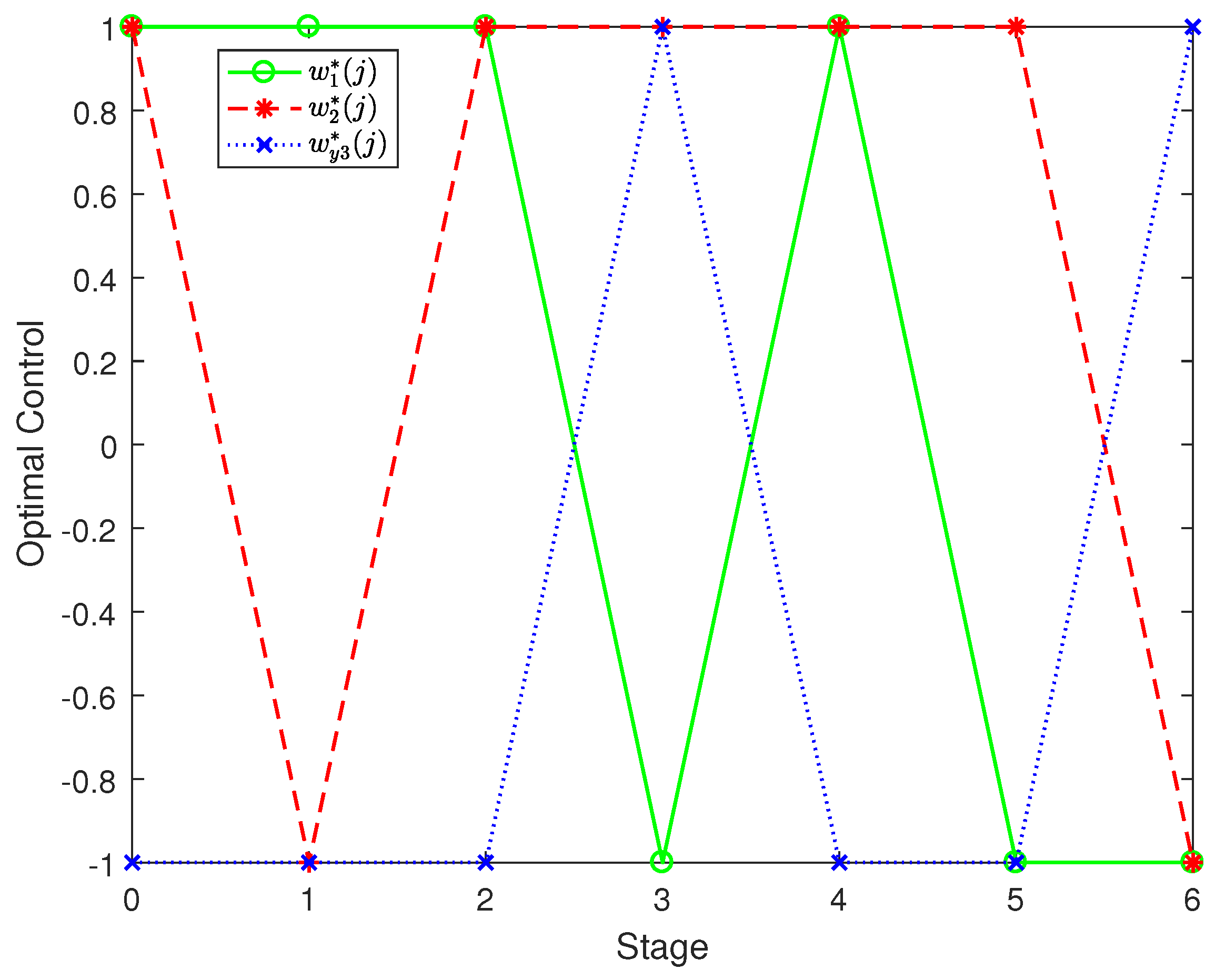
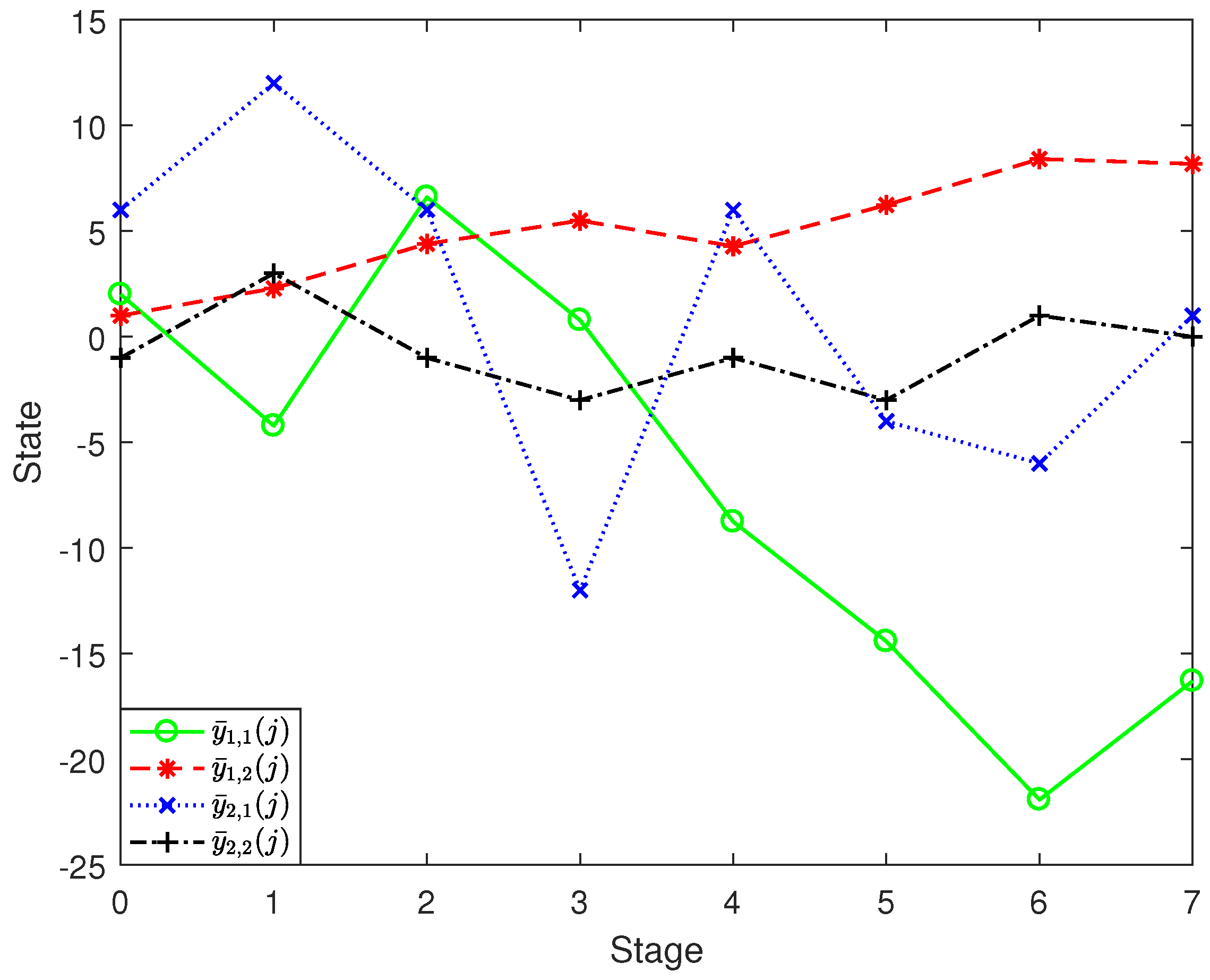
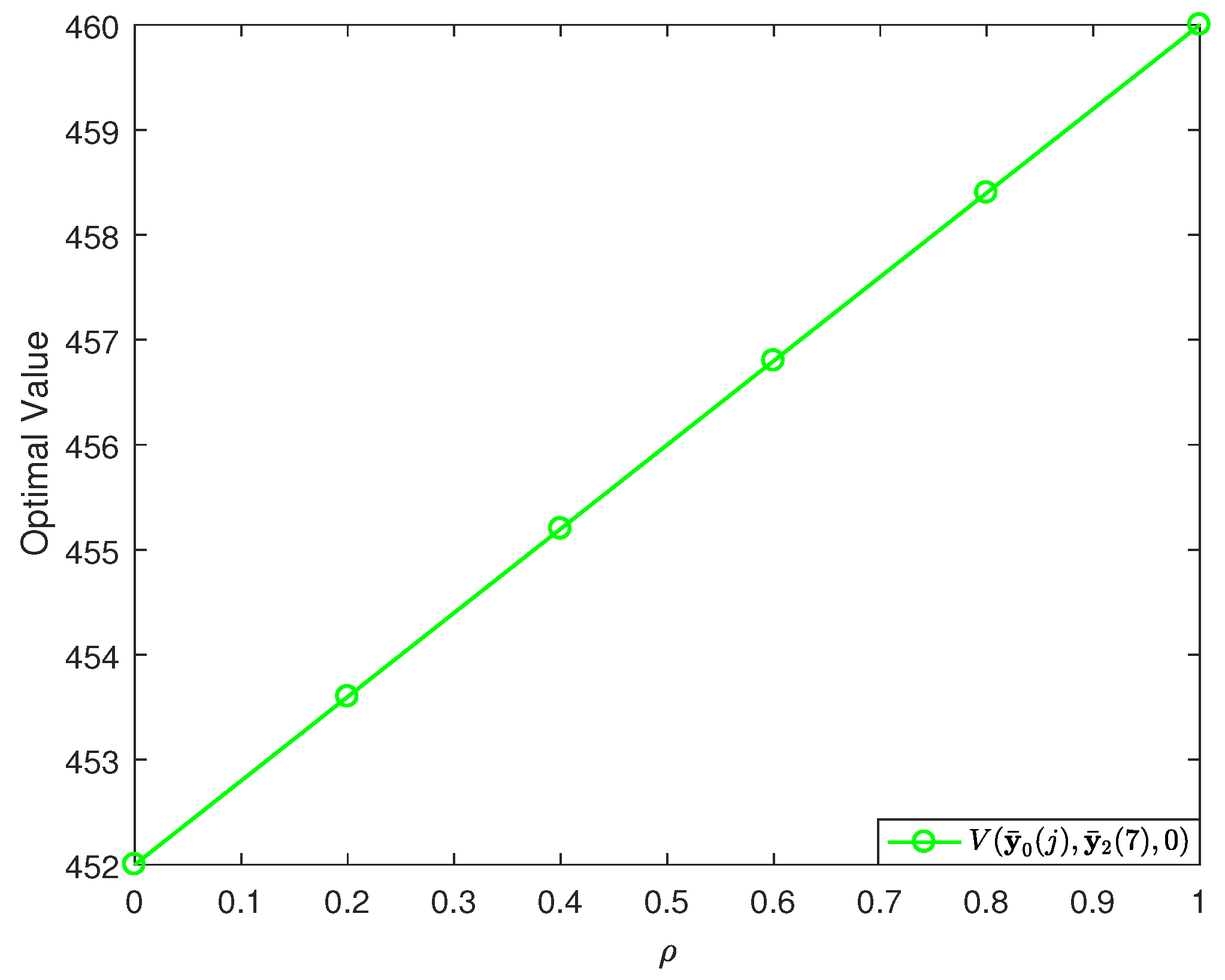
6. Numerical Example

Extensive research has been conducted in the field of power system control by numerous scholars [4,28,29]. To demonstrate the practical relevance and effectiveness of our theoretical framework, we present a physically motivated numerical example inspired by power system control:

$$\begin{array}{c}\hfill \left\{\begin{array}{c}V\left(\mathit{y}\right(0),\mathit{y}(7),0)\hfill \\ =\underset{\stackrel{\mathit{w}\left(j\right)\in {[-1,1]}^3}{0\le j\le 6}}{max}\left\{\rho {\left[{\displaystyle \sum _{j=0}^6}{\mathit{\varphi }}_j^{\mathrm{T}}\mathit{y}\left(j\right)+{\mathit{\varphi }}_7^{\mathrm{T}}\mathit{y}\left(7\right)\right]}_{sup}\left(\alpha \right)+(1-\rho ){\left[{\displaystyle \sum _{j=0}^6}{\mathit{\varphi }}_j^{\mathrm{T}}\mathit{y}\left(j\right)+{\mathit{\varphi }}_7^{\mathrm{T}}\mathit{y}\left(7\right)\right]}_{inf}\left(\alpha \right)\right\}\hfill \\ \mathrm{s}.\mathrm{t}.\hfill \\ \mathit{E}\mathit{y}(j+1)=\mathit{H}\mathit{y}\left(j\right)+\mathbf{\Pi }\mathit{w}\left(j\right)+\mathit{D}{\mathit{\xi }}_j,\hfill \\ j=0,1,2,\cdots ,6,\hfill \end{array}\right.\end{array}$$

(37)

where

$$\begin{array}{cc}\hfill & \mathit{E}=\left[\begin{array}{cccc}1& 0& 0& 0\\ 0& 0& 1& 0\\ 0& 0& 1& -1\\ 0& 0& 0& 0\end{array}\right],\mathit{H}=\left[\begin{array}{cccc}1& 1& 1& -3\\ 0& -1& 0& 1\\ 0& 0& 1& 0\\ 0& 0& 0& -1\end{array}\right],\mathbf{\Pi }=\left[\begin{array}{ccc}-1& 1& 2\\ 2& 3& -1\\ -1& 2& 3\\ 1& -2& 0\end{array}\right],\mathit{D}=\left[\begin{array}{cccc}-1& -2& 1& 0\\ 0& 2& -2& 0\\ 0& 2& -2& 0\\ 0& 0& 0& 0\end{array}\right].\hfill \end{array}$$

The matrix $\mathit{E}$ captures the singular dynamics of the system, which can represent, for example, instantaneous voltage drops caused by faults in power networks. The uncertainty vectors ${\mathit{\xi }}_j={({\xi }_j^1,{\xi }_j^2,{\xi }_j^3,{\xi }_j^4)}^{\mathrm{T}}$ model uncertain external inputs such as fluctuating loads or component tolerances. Each ${\xi }_j^i$ ($i=1,2,3,4$, $j=0,1,\cdots ,6$) is an independent linear uncertain variable following the uncertainty distribution $\mathcal{L}(-{\displaystyle \frac{1}{2}},{\displaystyle \frac{1}{2}})$. These ${\xi }_j^{i_w}$ are independent linear uncertain variables. The state weighting vectors are

$$\begin{array}{cc}\hfill & \left[\begin{array}{c}{\mathit{\varphi }}_0^{\mathrm{T}}\\ {\mathit{\varphi }}_1^{\mathrm{T}}\\ {\mathit{\varphi }}_2^{\mathrm{T}}\\ {\mathit{\varphi }}_3^{\mathrm{T}}\\ {\mathit{\varphi }}_4^{\mathrm{T}}\\ {\mathit{\varphi }}_5^{\mathrm{T}}\\ {\mathit{\varphi }}_6^{\mathrm{T}}\end{array}\right]=\left[\begin{array}{cccc}4& 6& -3& 2\\ 3& 5& 4& 9\\ -2& 6& 3& 9\\ 3& -5& -5& 6\\ 4& 4& 7& 5\\ 5& 2& 5& -7\\ 7& -4& 6& 3\end{array}\right],\hfill \end{array}$$

and ${\mathit{\varphi }}_7^{\mathrm{T}}=(1,-1,{\displaystyle \frac{1}{2}},{\displaystyle \frac{3}{2}})$.

First, we have

$$\begin{array}{c}\hfill det(x\mathit{E}-\mathit{H})=det\left[\begin{array}{cccc}x-1& -1& -1& 3\\ 0& 1& x& -1\\ 0& 0& x-1& -x\\ 0& 0& 0& 1\end{array}\right]=x^2-2x+1\not\equiv 0,\end{array}$$

and $degdet(x\mathit{E}-\mathit{H})=2<rank\left(\mathit{E}\right)=3$, i.e., the system under consideration belongs to the category of uncertain singular non-causal systems. There are nonsingular matrices

$$\begin{array}{c}\hfill \mathit{F}=\left[\begin{array}{cccc}-1& -1& 0& 2\\ 0& 0& -{\displaystyle \frac{1}{2}}& -{\displaystyle \frac{1}{2}}\\ 0& -1& 1& -2\\ 0& 0& 0& -1\end{array}\right],\mathit{M}=\left[\begin{array}{cccc}-1& 2& 0& -1\\ 0& 2& 1& -2\\ 0& -2& 0& 1\\ 0& 0& 0& 1\end{array}\right],\end{array}$$

such that

$$\begin{array}{c}\hfill \mathit{F}\mathit{E}\mathit{M}=\left[\begin{array}{cccc}1& 0& 0& 0\\ 0& 1& 0& 0\\ 0& 0& 0& -1\\ 0& 0& 0& 0\end{array}\right],\mathit{F}\mathit{H}\mathit{M}=\left[\begin{array}{cccc}1& 0& 0& 0\\ 0& 1& 0& 0\\ 0& 0& 1& 0\\ 0& 0& 0& 1\end{array}\right],\mathit{F}\mathbf{\Pi }=\left[\begin{array}{ccc}1& -8& -1\\ 0& 0& -1.5\\ -5& 3& 4\\ -1& 2& 0\end{array}\right],\mathit{F}\mathit{D}=\left[\begin{array}{cccc}1& 0& 1& 0\\ 0& -1& 1& 0\\ 0& 0& 0& 0\\ 0& 0& 0& 0\end{array}\right].\end{array}$$

We obtain

$$\begin{array}{cc}\hfill & {\mathit{E}}_2=\left[\begin{array}{cc}0& -1\\ 0& 0\end{array}\right],{\mathit{H}}_1=\left[\begin{array}{cc}1& 0\\ 0& 1\end{array}\right],{\mathbf{\Pi }}_1=\left[\begin{array}{ccc}1& -8& -1\\ 0& 0& -1.5\end{array}\right],{\mathbf{\Pi }}_2=\left[\begin{array}{ccc}-5& 3& 4\\ -1& 2& 0\end{array}\right],\hfill \\ \hfill & {\mathit{D}}_1=\left[\begin{array}{cccc}1& 0& 1& 0\\ 0& -1& 1& 0\end{array}\right],{\mathit{D}}_2=\left[\begin{array}{cccc}0& 0& 0& 0\\ 0& 0& 0& 0\end{array}\right],\hfill \end{array}$$

and

$$\begin{array}{c}\hfill {\mathit{M}}_1=\left[\begin{array}{cc}-1& 2\\ 0& 2\\ 0& -2\\ 0& 0\end{array}\right],{\mathit{M}}_2=\left[\begin{array}{cc}0& -1\\ 1& -2\\ 0& 1\\ 0& 1\end{array}\right].\end{array}$$

Under the condition ${\mathit{D}}_2=\mathbf{0}$, the problem (37) corresponds to

$$\begin{array}{c}\hfill \left\{\begin{array}{c}\overline{V}({\overline{\mathit{y}}}_1\left(0\right),{\overline{\mathit{y}}}_2\left(7\right),0)\hfill \\ =\underset{\stackrel{\mathit{w}\left(j\right)\in {[-1,1]}^3}{0\le j\le 6}}{max}\{\rho {\left[{\displaystyle \sum _{j=0}^6}{\mathit{\varphi }}_j^{\mathrm{T}}[{\mathit{M}}_1{\overline{\mathit{y}}}_1\left(j\right)+{\mathit{M}}_2{\overline{\mathit{y}}}_2\left(j\right)]+{\mathit{\varphi }}_7^{\mathrm{T}}[{\mathit{M}}_1{\overline{\mathit{y}}}_1\left(7\right)+{\mathit{M}}_2{\overline{\mathit{y}}}_2\left(7\right)]\right]}_{sup}\left(\alpha \right)\hfill \\ +(1-\rho ){\left[{\displaystyle \sum _{j=0}^6}{\mathit{\varphi }}_j^{\mathrm{T}}[{\mathit{M}}_1{\overline{\mathit{y}}}_1\left(j\right)+{\mathit{M}}_2{\overline{\mathit{y}}}_2\left(j\right)]+{\mathit{\varphi }}_7^{\mathrm{T}}[{\mathit{M}}_1{\overline{\mathit{y}}}_1\left(7\right)+{\mathit{M}}_2{\overline{\mathit{y}}}_2\left(7\right)]\right]}_{inf}\left(\alpha \right)\}\hfill \\ \mathrm{s}.\mathrm{t}.\hfill \\ {\overline{\mathit{y}}}_1(j+1)={\mathit{H}}_1{\overline{\mathit{y}}}_1\left(j\right)+{\mathbf{\Pi }}_1\mathit{w}\left(j\right)+{\mathit{D}}_1{\mathit{\xi }}_j,\hfill \\ {\overline{\mathit{y}}}_2\left(j\right)={\mathit{E}}_2{\overline{\mathit{y}}}_2(j+1)-{\mathbf{\Pi }}_2\mathit{w}\left(j\right),\hfill \\ j=0,1,2,\cdots ,6.\hfill \end{array}\right.\end{array}$$

(38)

The objective function integrates energy loss and terminal cost, reflecting voltage stability at the final stage $J=7$). The Hurwicz criterion plays a central role by allowing operators to balance risk and reward, which is crucial for effective power grid management. By setting the weight parameter $\rho =0.6$ and confidence level $\alpha =0.7$, the framework emphasizes maximizing power supply under moderate risk, thereby enhancing system resilience without incurring excessive uncertainty exposure. Given the initial state ${\overline{\mathit{y}}}_1\left(0\right)={(2,1)}^{\mathrm{T}}$ and terminal state ${\overline{\mathit{y}}}_2\left(7\right)={(1,0)}^{\mathrm{T}}$, the optimal solutions to problem (38) are obtained by applying Algorithm 1. The resulting values are summarized in

Table 1. The optimal results of problem (38).

Stage	${\left({\mathit{l}}^{\mathit{j}}\right)}^{\mathbf{T}}$	${\left({\mathit{u}}^{\mathit{j},1}\right)}^{\mathbf{T}}$	${\left({\mathit{w}}^{*}\left(\mathit{j}\right)\right)}^{\mathbf{T}}$	${\left({\overline{\mathit{y}}}_1\left(\mathit{j}\right)\right)}^{\mathbf{T}}$	${\left({\overline{\mathit{y}}}_2\left(\mathit{j}\right)\right)}^{\mathbf{T}}$	$\mathit{V}({\overline{\mathit{y}}}_1\left(\mathit{j}\right),{\overline{\mathit{y}}}_2\left(7\right),\mathit{j})$
0	$(10,40,-33)$		$(1,1,-1)$	$(2,1)$	$(6,-1)$	$456.8000$
1	$(27,-31,-25)$	$(-6,12,0)$	$(1,-1,-1)$	$(-4.2183,2.2909)$	$(12,3)$	$409.5418$
2	$(29,2,-30)$	$(-5,10,0)$	$(1,1,-1)$	$(6.6022,4.3935)$	$(6,-1)$	$330.7113$
3	$(-21,31,21)$	$(-6,12,0)$	$(-1,1,1)$	$(0.7821,5.4972)$	$(-12,-3)$	$255.1172$
4	$(15,28,-17)$	$(5,-10,0)$	$(1,1,-1)$	$(-8.7544,4.2826)$	$(6,-1)$	$211.7428$
5	$(-3,32,-6)$	$(-4,8,0)$	$(-1,1,-1)$	$(-14.4185,6.2345)$	$(-4,-3)$	$190.7907$
6	$(-5,-48,2)$	$(-2,4,0)$	$(-1,-1,1)$	$(-21.9123,8.4115)$	$(-6,1)$	$106.4245$
7				$(-16.2940,8.1806)$	$(1,0)$	$-30.3860$

.

Given that the nilpotency of the matrix ${\mathit{E}}_2$ is 2, we can deduce that ${\mathit{u}}^{j,j}=-{\sum }_{k=1}^j{\mathit{\varphi }}_{j-k}^{\mathrm{T}}{\mathit{M}}_2{\mathit{E}}_2^k{\mathbf{\Pi }}_2={\mathit{u}}^{j,1}$, as is evident from column 3 of Table 1. Additionally, the trajectories corresponding to the optimal controls ${\mathit{w}}^{*}\left(j\right)={(w_1^{*}\left(j\right),w_2^{*}\left(j\right),w_3^{*}\left(j\right))}^{\mathrm{T}}$ are illustrated in Figure 2, where $w_1^{*}\left(j\right),w_2^{*}\left(j\right)$, and $w_3^{*}\left(j\right)$ represent reactive power regulation, active power regulation, and energy storage output, respectively. The numerical values are listed in column 4 of Table 1. During stages $j=0$ to 2, the control strategy operates as follows: When $w_1=1$, reactive power is rapidly injected to mitigate voltage sags occurring during the closing process. Meanwhile, active power is adjusted sequentially with $w_2=1,-1,1$ to effectively respond to sudden load variations. Simultaneously, when $w_3=-1$, the energy storage system discharges to compensate for the initial energy deficit in the system. During stages $j=3$ to 6, the control logic transitions to a new phase: based on voltage feedback, $w_1$ switches through the sequence $-1,1,-1,-1$, reversing the direction of reactive power injection to prevent overvoltage. Concurrently, active power is consistently supplied with $w_2=1,1,1,-1$ to support generator acceleration. At the same time, with $w_3=1,-1,-1,1$, the energy storage system charges to absorb surplus energy and suppress over-frequency events, thus ensuring stable system operation.

The trajectories of the states ${\overline{\mathit{y}}}_1\left(j\right)$ and ${\overline{\mathit{y}}}_2\left(j\right)$ are illustrated in Figure 3, with the corresponding numerical data provided in columns 5 and 6 of Table 1, respectively. It is worth noting that the state ${\overline{y}}_{2,1}\left(j\right)$ experiences substantial variations. This is because it is governed by the optimal control, as described by the relation ${\overline{y}}_{2,1}\left(j\right)=-8w_1^{*}\left(j\right)+2w_2^{*}\left(j\right)+5w_3^{*}\left(j\right)$.

According to the simulation results, the optimal value $V({\overline{\mathit{y}}}_1\left(0\right),{\overline{\mathit{y}}}_2\left(7\right),0)$ exhibits a clear linear increasing trend with respect to $\rho$, as illustrated in

Table 2. Optimal value $V({\overline{\mathit{y}}}_1\left(0\right),{\overline{\mathit{y}}}_2\left(7\right),0)$ corresponding to various $\rho$ levels.

$\mathit{\rho }$	0	0.2	0.4	0.6	0.8	1
$V({\overline{\mathit{y}}}_1\left(0\right),{\overline{\mathit{y}}}_2\left(7\right),0)$	452	453.6000	455.2000	456.8000	458.4000	460.0000

and Figure 4.

As shown in Table 2, when $\rho =0$ the strategy considers only the pessimistic scenario (i.e., the worst case), resulting in the minimum value of the objective function, reflecting a conservative control approach. In contrast, when $\rho =1$, the strategy focuses solely on the optimistic scenario, leading to the maximum objective value, which corresponds to an aggressive control policy. For intermediate values of $\rho$ (e.g., $\rho =0.6$) the strategy achieves a trade-off between risk and performance. The objective value increases linearly with the optimism weight, which is consistent with the convex combination property of the Hurwicz criterion. Analogous to the methodology applied in the preceding sections, Algorithm 2 can be systematically employed to solve problem (25). This algorithmic approach leverages the problem’s structural properties to compute the optimal controls across varying optimism-pessimism spectra, ensuring both computational tractability and theoretical rigor.

7. Conclusions

This study aims to advance the theoretical frontier of uncertain optimal control by focusing on problems arising in uncertain singular non-causal systems within the framework of the Hurwicz criterion. As a distinctive class of systems, uncertain singular non-causal systems can be transformed into equivalent subsystems through carefully designed mathematical transformations. Leveraging the rigor of equivalent transformation principles, the original complex problem is reformulated into a more tractable structure comprising uncertain forward and backward subsystems. Subsequently, this study integrates dynamic programming and uncertainty theory to meticulously construct a recurrence equation specifically designed to tackle such problems. Through the recurrence equation, the problems can be systematically and step-by-step decomposed and solved. As special cases in this study, we pay particular attention to the optimal control problems of linear and nonlinear uncertain singular non-causal systems. For these complex scenarios, based on the established recurrence equation, we have successfully derived the precise analytical expressions for the optimal control of such problems, and also determined the related optimal values. To validate and illustrate the practical applicability of the proposed framework, a carefully designed numerical example is provided. This example offers a clear and comprehensive demonstration of how the proposed approach can be employed to solve uncertain singular non-causal control problems under the Hurwicz criterion.

Although this study has achieved significant milestones, several promising directions remain for future research. These include extending the framework to singular systems exhibiting strong nonlinear dynamics and complex uncertainty interactions; developing data-driven dynamic adjustment strategies for $\rho$ to optimize risk preferences in real time; conducting field validations in areas such as real-time grid frequency control and high-speed signal reconstruction to deepen the integration of theory and practice; and exploring new preference aggregation mechanisms for complex decision-making scenarios. This research not only provides theoretical tools for the control of uncertain singular non-causal systems but also offers methodological references for solving similar uncertain decision problems in interdisciplinary fields through its structured research approach.

References

1. Rosenbrock, H.H. Structural properties of linear dynamical systems. Int. J. Control 1974, 20, 191–202. [Google Scholar] [CrossRef]
2. Luenberger, D.G.; Arbel, A. Singular dynamic Leontief systems. Econometrica 1977, 45, 991–995. [Google Scholar] [CrossRef]
3. Cobb, D. Controllability, observability, and duality in singular systems. IEEE Trans. Autom. Control 1984, 29, 1076–1082. [Google Scholar] [CrossRef]
4. Dai, L. Singular Control Systems; Springer: Berlin/Heidelberg, Germany, 1989. [Google Scholar]
5. Lukashiv, T.; Malyk, I.V.; Hemedan, A.A.; Satagopam, V.P. Optimal control of stochastic dynamic systems with semi-Markov parameters. Symmetry 2025, 17, 498. [Google Scholar] [CrossRef]
6. Shu, Y.; Li, B. Linear-quadratic optimal control for discrete-time stochastic descriptor systems. J. Ind. Manag. Optim. 2022, 18, 1583–1602. [Google Scholar] [CrossRef]
7. Vlasenko, L.A.; Rutkas, A.G.; Semenets, V.V.; Chikrii, A.A. Stochastic optimal control of a descriptor system. Cybern. Syst. Anal. 2020, 56, 204–212. [Google Scholar] [CrossRef]
8. Li, Y.; Ma, S. Finite and infinite horizon indefinite linear quadratic optimal control for discrete-time singular Markov jump systems. J. Frankl. Inst. 2021, 358, 8993–9022. [Google Scholar] [CrossRef]
9. Liu, B. Uncertainty Theory, 2nd ed.; Springer: Berlin/Heidelberg, Germany, 2007. [Google Scholar]
10. Liu, B. Uncertainty Theory, 4th ed.; Springer: Berlin/Heidelberg, Germany, 2015. [Google Scholar]
11. Li, B.; Zhang, R.; Sun, Y. Multi-period portfolio selection based on uncertainty theory with bankruptcy control and liquidity. Automatica 2023, 147, 110751. [Google Scholar] [CrossRef]
12. Liu, Y.; Zhou, L. Modeling RL electrical circuit by multifactor uncertain differential equation. Symmetry 2021, 13, 2103. [Google Scholar] [CrossRef]
13. Mohammed, P.O. A generalized uncertain fractional forward difference equations of Riemann-Liouville type. J. Math. Res. 2019, 11, 43–50. [Google Scholar] [CrossRef]
14. Zhu, Y. Uncertain Optimal Control; Springer Nature: Singapore, 2019. [Google Scholar]
15. Shu, Y.; Zhu, Y. Optimistic value based optimal control for uncertain linear singular systems and application to a dynamic input-output model. ISA Trans. 2017, 71, 235–251. [Google Scholar] [CrossRef] [PubMed]
16. Deng, L.; You, Z.; Chen, Y. Optimistic value model of multidimensional uncertain optimal control with jump. Eur. J. Control 2018, 39, 1–7. [Google Scholar] [CrossRef]
17. Yang, X.; Gao, J. Linear-quadratic uncertain differential games with application to resource extraction problem. IEEE Trans. Fuzzy Syst. 2016, 24, 819–826. [Google Scholar] [CrossRef]
18. Chen, X.; Zhu, Y. Optimal control for uncertain random singular systems with multiple time-delays. Chaos Solitons Fractals 2021, 152, 111371. [Google Scholar] [CrossRef]
19. Chen, X.; Zhu, Y.; Sheng, L. Optimal control for uncertain stochastic dynamic systems with jump and application to an advertising model. Appl. Math. Comput. 2021, 407, 126337. [Google Scholar] [CrossRef]
20. Latunde, T.; Bamigbola, O.M. Uncertain optimal control model for management of net risky capital asset. IOSR J. Math. 2016, 12, 22–30. [Google Scholar]
21. Shu, Y.; Zhu, Y. Stability analysis of uncertain singular systems. Soft Comput. 2018, 22, 5671–5681. [Google Scholar] [CrossRef]
22. Shu, Y.; Li, B.; Zhu, Y. Optimal control for uncertain discrete-time singular systems under expected value criterion. Fuzzy Optim. Decis. Mak. 2021, 20, 331–364. [Google Scholar] [CrossRef]
23. Shu, Y.; Zhu, Y. Stability and optimal control for uncertain continuous-time singular systems. Eur. J. Control 2017, 34, 16–23. [Google Scholar] [CrossRef]
24. Chen, X.; Cao, Z.; Zhang, Z. Linear quadratic optimal control and zero-sum game for uncertain time-delay systems based on pessimistic value. Eur. J. Control 2025, 84, 101224. [Google Scholar] [CrossRef]
25. Shu, Y.; Sheng, L. Hurwicz criterion based optimal control model for uncertain descriptor systems with an application to industrial management. J. Ind. Manag. Optim. 2023, 19, 6054–6081. [Google Scholar] [CrossRef]
26. Shu, Y. Optimal control for discrete-time descriptor noncausal systems. Asian J. Control 2021, 23, 1885–1899. [Google Scholar] [CrossRef]
27. Hurwicz, L. Some specification problems and application to econometric models. Econometrica 1951, 19, 343–344. [Google Scholar]
28. Pierre, D.A. A perspective on adaptive control of power systems. IEEE Trans. Power Syst. 2007, 2, 387–395. [Google Scholar] [CrossRef]
29. Kwatny, H.G.; Miu-Miller, K. Power System Dynamics and Control; Springer: New York, NY, USA, 2016. [Google Scholar]
Figure 1. Schematic of the developed methodology for the Hurwicz-type optimal control problem of uncertain singular non-causal systems.
Symmetry 17 01130 g001
Figure 2. Trajectory concerning the optimal control w * ( j ) = ( w 1 * ( j ) , w 2 * ( j ) , w 3 * ( j ) ) T .
Symmetry 17 01130 g002
Figure 3. Trajectories concerning states y ¯ 1 ( j ) = ( y ¯ 1 , 1 ( j ) , y ¯ 1 , 2 ( j ) ) T , y ¯ 2 ( j ) = ( y ¯ 2 , 1 ( j ) , y ¯ 2 , 2 ( j ) ) T .
Symmetry 17 01130 g003
Figure 4. Trajectory concerning the optimal value V ( y ¯ 1 ( 0 ) , y ¯ 2 ( 7 ) , 0 ) .
Symmetry 17 01130 g004